Machine Learning-Driven Portfolio Optimization Using Money Flow Index-Based Sentiment Signals

Abstract

Market indices serve as a benchmark for performance comparison, guide asset allocation decisions, and reflect overall market sentiment and economic conditions, thereby influencing investment strategies by representing a segment of the market. Unquestionably, investor sentiment impacts price movement. In this paper, the objectives were to study the effectiveness of the Money Flow Index (MFI) in enhancing the performance of predictive analysis by capturing market psychology, developing an investment strategy, and analyzing the performance of the method mentioned. This study applies machine learning algorithms with technical indicators and optimizes portfolio allocation based on three notable market indices in Southeast Asia (SEA): SET50 in Thailand, STI in Singapore, and VN30 in Vietnam. Firstly, we combined technical indicators with machine learning—Support Vector Classifier (SVC), Random Forest (RF), and Extreme Gradient Boosting (XGBoost)—by comparing datasets with and without MFI over the period from 2013 to 2023. The results showed that XGBoost with MFI delivered the best predictive performance across three indices. These findings indicate that MFI significantly enhances prediction accuracy, even during volatile market conditions (COVID-19). Additionally, the predictions were integrated into the Markowitz Mean-Variance (MV) model to construct an optimal portfolio, which was then benchmarked against an equal-weight portfolio (1/N). Ultimately, the findings demonstrate that incorporating the machine learning predictions into the MV framework efficiently generates wealth.

1. Introduction

In the modern capitalist era, capital and stock markets serve as the essential mechanisms for wealth preservation and growth. Over the past decade, capital markets in fast-growing regions, such as Southeast Asia (SEA), have become highly attractive options for investors seeking portfolio diversification and robust long-term returns. Three stock market indices that highlight the SEA region’s potential are the Singapore Straits Times Index (STI), which tracks the performance of the Singapore stock exchange; the Stock Exchange of Thailand 50 Index (SET50), which represents the top 50 companies listed on the Thai bourse; and the VN30 Index, a rising star in the region and the main benchmark for the Ho Chi Minh Stock Exchange in Vietnam. However, various elements influence bullish and bearish regimes in these areas, including economic factors and investor sentiment. It is then a significant challenge to navigate these markets.

In the current financial landscape, various analytical tools are available for investors to achieve the goal of outperforming the market while minimizing risk. One of the most powerful tools is machine learning (ML). Many investors are now using machine learning models (e.g., Support Vector Machine (SVM), Random Forest (RF), Artificial Neural Network (ANN), and Extreme Gradient Boosting (XGBoost)) to build models that help identify complex, non-linear patterns in financial time series (Asad, 2015; Chaengkham & Wianwiwat, 2021; Sangsawai & Sutivong, 2023; Yuan et al., 2020). However, applying only machine learning presents an incredibly challenging task due to market uncertainties. Therefore, applying more than one method to address market variance is crucial for advancing predictive performance. One of the most well-known and frequently selected approaches is technical indicators, which consist of mathematical calculations derived from historical price and volume data. These indicators provide valuable insights into widespread aspects of the supply and demand of securities as well as market psychology. For over a decade, the combination of ML algorithms with traditional technical indicators to forecast stock price movements has been continuously proposed. Commonly utilized technical indicators include the Simple Moving Average (SMA), Relative Strength Index (RSI), Exponential Moving Average (EMA), and Moving Average Convergence Divergence (MACD) (Ayala et al., 2021; Basak et al., 2019; Kumbure et al., 2022; Misra & Chaurasia, 2020; Parray et al., 2020; Phuoc et al., 2024; Saetia & Yokrattanasak, 2023; S. Wang, 2020). Furthermore, financial markets also have a diverse range of market participants with different preferences for investment patterns, risk acceptance, and emotional responses to market conditions. This diversity implies that each investor’s attitude and trading behavior can influence the overall movement of the market index. Several studies show that investors’ sentiment is linked to the movement of the market, particularly in the context of high volatility and large market size (Fonou-Dombeu et al., 2024; Gao et al., 2022; Kumari & Mahakud, 2016; Lee et al., 2002; Moodley et al., 2024; Narayanasamy et al., 2023; Ph & Rishad, 2020; QuantifiedTrading, 2025). Moreover, the behavioral patterns observed in investors tend to be relatively consistent in sentiment and volume, driving short-lived trading activities. Market sentiment is easily affected by unforeseen events or crises. To capture these rapid shifts in sentiment, the Money Flow Index (MFI) serves as a robust tool. It closely aligns with sentiment indices by reflecting the trading actions of market actors and serves as an early sign of potential price shifts (Chen et al., 2010; Marek & Marková, 2020; Phuong, 2021; Ye et al., 2018).

Although ML is widely used in financial forecasting, there are still some areas where more research is needed. First, the Money Flow Index (MFI) has not been systematically integrated as the primary feature of ML forecasting models. Second, most existing research focuses on measuring classification accuracy, which fails to translate these forecasting signals into optimized financial portfolios. Finally, empirical research that simultaneously combines sentiment analysis, machine learning forecasting, and portfolio optimization is scarce for the STI, SET50, and VN30 indices.

To address these research gaps, identifying the Money Flow Index (MFI), an indicator signaling potential price changes from overbought or oversold conditions, to act as a proxy for investor sentiment is crucial. Empirical evidence indicates that MFI-based strategies outperform traditional buy-and-hold methods, particularly when investor sentiment significantly influences stock fundamental returns during periods of high market volatility (Marek & Marková, 2020; Phuong, 2021). Moreover, developing a dynamic framework that incorporates technical indicators, especially capturing investors’ emotions through MFI, alongside multiple machine learning algorithms and portfolio optimization models, is also important. This integrated approach leverages predictive capabilities to construct portfolio models that bridge the gap between theoretical quantitative finance and high-performance practical applications. Recent research supports a hybrid decision-making framework where machine learning (ML) forecasting is directly fed into modern portfolio theory, such as optimizing the Markowitz Mean-Variance (MV) model to achieve superior risk-adjusted returns (Chaweewanchon & Chaysiri, 2022; Ma et al., 2021; Paiva et al., 2019; W. Wang et al., 2020; Yu et al., 2020).

Hence, the objective of this research is to propose an alternative approach to support investors’ decisions in minimizing risk while maximizing profits. This study focuses on the development of an integrated, end-to-end investment framework that explicitly incorporates investor sentiment (via the Money Flow Index (MFI)) alongside traditional technical indicators into machine learning predictions and portfolio optimization within the Southeast Asian context. Based on this objective, an experimental study is implemented by gathering historical index data from the STI, VN30, and SET50 from 2013 to 2023, including the COVID-19 pandemic period. Technical indicators, including MFI for capturing investor sentiment, are fed into machine learning algorithms. Three selected popular supervised machine learning algorithms were selected for a comparative performance analysis: Random Forest (RF), Support Vector Machine (SVM), and Extreme Gradient Boosting (XGBoost) (Bustos & Pomares-Quimbaya, 2020; Dev & Bhatnagar, 2024; Mokhtari et al., 2021; Worasucheep, 2022). Each possesses distinct strengths and weaknesses, making them suitable for several types of classification and regression problems depending on the characteristics of the data. Finally, the predictive outputs are used to construct optimal portfolio strategies using the Markowitz Mean-Variance optimization (MV), a widespread approach in portfolio theory (Ferreira et al., 2021), and evaluated against the benchmark model (an equal-weight approach (1/N)).

2. Methodology

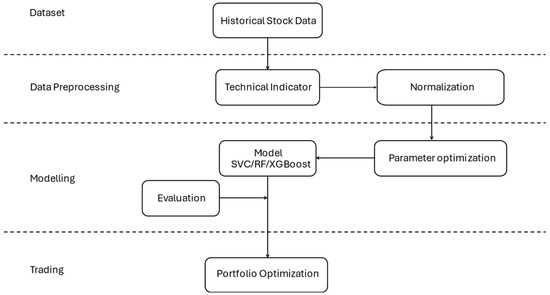
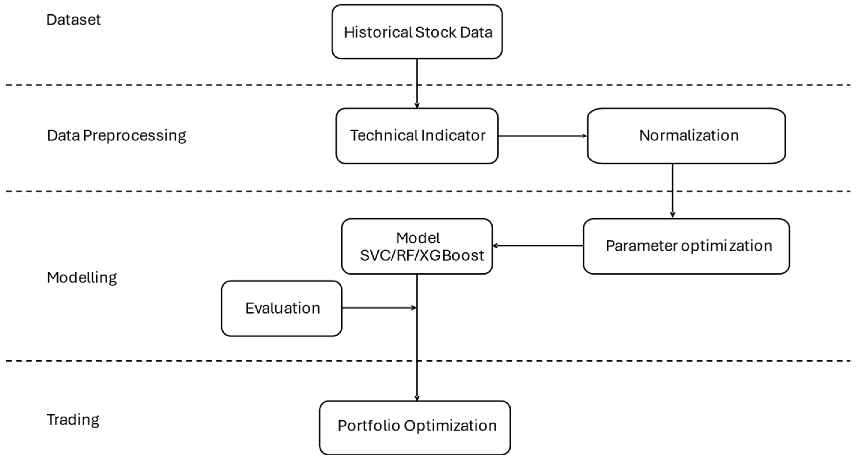
The previous section discussed engaging research, which provides a theoretical basis for the established model. This section introduces the proposed techniques for the prediction of stock price movement. This research mainly focuses on two key stages: (1) stock movement prediction and (2) optimized portfolio with relative to the portfolio’s variance. Figure 1 illustrates the overall research workflow.

Figure 1. Diagram of the proposed approach.

2.1. Dataset

The historical price data used in this study was taken from the Investing website https://www.investing.com (accessed on 14 September 2025), which involves open, high, low, close, and volume as extracted data from 2013 to 2023, a 10-year period for three stock indices from Southeast Asia: (1) The Straits Times Index (STI), which tracks the performance of the top 30 companies listed on the Singapore Exchange (SGX); (2) the SET50 index, which reflects the price movement of the top 50 stocks in the Stock Exchange of Thailand (SET); and (3) the VN30 Index of Vietnam, which is the rising star market in Southeast Asia and also tracks the performance of the top 30 companies listed on the Vietnam Stock Exchange. A summary of the data, which includes the starting and ending dates, is provided, followed by the total number of observations, as shown in Table 1.

Table 1. Summary of the index data.

Country	Symbol	Start	End	Observations
Thailand	SET50	15 Febuary 2013	28 December 2023	2646
Singapore	STI	19 Febuary 2013	29 December 2023	2725
Vietnam	VN30	22 Febuary 2013	29 December 2023	2713

2.2. Data Preprocessing

Model performance is influenced by the input variables. The efficiency of predictive models employed in both short-term day trading and long-term investment strategies is contingent upon the precision and arrangement of input variables.

This research employed technical indicators with historical price data to generate a feature set for the classifiers, including (1) SMA10, (2) EMA12, (3) MACD (12,26), (4) MOM10, (5) RSI14, and (6) MFI14. The specific look-back periods for each technical indicator utilized as input variables are detailed in Table 2.

Table 2. Technical indicator input variables.

Technical Indicators	Time Period
SMA	10 days
EMA	12 days
MACD	12, 26 days
MOM	10 days
RSI	14 days
MFI	14 days

As historical data is continuous data, which has an unbroken continuum without separations between values, stock movement direction is explainable as discrete data as a target variable, which is produced by classifying the closing price in the form of +1 or 0, represented by +1 for an upward trend and 0 for a downward trend the next day. The target variable reflects the stock movement as rising or falling. Aligning with stock movement prediction, the signal will be generated.

To transform continuous price data into a binary classification target, we first calculate the daily percentage change ($r_t)$ using the closing price ($P_t)$ and the previous day’s closing price, $P_{t-1}$,

$$r_t={\displaystyle \frac{P_t-P_{t-1}}{P_{t-1}}}$$

(1)

Once the percentage change is calculated, a threshold of zero is applied to the forward-looking return, $r_{t+1},$ to generate the binary target variable, $y_t$. In this framework, any strictly positive future move is labeled as a bullish movement (1), and any zero or negative move is labeled as a bearish movement (0). The labeling function is defined as

$$y_t=\left\{\begin{array}{c}1if{r}_{t+1}>0\\ 0if{r}_{t+1}\le 0\end{array}\right.$$

(2)

2.3. Technical Indicators

Technical indicators, listed in Table 2, are tools used to predict trends in the movement of the price of commodities. These models are synthesized from primary market variables such as trading volume and price action (including opening, closing, and price range across specific timeframes). By mapping these cyclical behaviors against past market activity, one can predict future directions. Technical signals are believed to be effective determinants for the timing of asset acquisition and liquidation (Fredrik, 2007; Prashanth et al., 2023). Our trading approach generates revenue through using 6 current technical indicators. The technical indicators used in this study are explained below.

2.3.1. Simple Moving Average (SMA)

A moving average effectively smooths price series data, enhancing trend identification. This indicator is derived by calculating the average of closing prices over a specified period (N days). If the SMA is increasing, it indicates an uptrend, while a downward trend implies the opposite (Fredrik, 2007). The formula that follows is the SMA, shown below.

$$\mathrm{SMA}={\displaystyle \frac{\mathrm{sum}\mathrm{of}\mathrm{close}\mathrm{price}\mathrm{N}}{\mathrm{N}}}$$

(3)

2.3.2. Exponential Moving Average (EMA)

Exponential Moving Average (EMA) uses a weighting scheme that decays exponentially, thereby prioritizing recent data. As the window size increases, the relative weight assigned to the most recent price decreases, reducing the impact of immediate price shifts. This characteristic is particularly beneficial for offering a more timely reflection of trend shifts (Gorenc Novak & Velušček, 2016). The mathematical framework of EMA is

$${\mathrm{EMA}}_{\mathrm{t}}=\mathsf{\alpha }·{\mathrm{P}}_{\mathrm{t}}+\left(1-\mathsf{\alpha }\right)·{\mathrm{EMA}}_{\mathrm{t}-1}$$

(4)

where $\mathsf{\alpha }={\displaystyle \frac{2}{\mathrm{n}+1}},$ and ${\mathrm{P}}_{\mathrm{t}}$ is the current price.

2.3.3. Moving Average Convergence Divergence (MACD)

The MACD is a momentum-based trend indicator that tracks the convergence and divergence of two Exponential Moving Averages (Dongrey, 2022). The derivation of the MACD is divided into a two-stage process: initially calculating the primary MACD line and subsequently generating the MACD histogram to serve as a critical diagnostic tool for identifying changes in momentum strength and potential trend reversals within high-frequency trading data. The MACD line is the difference between the EMA of a shorter period and the EMA of a longer period (da Costa et al., 2015). By taking the difference between the 26-period EMA and the 12-period EMA, the signal line is commonly represented as a 9-period EMA of the MACD.

$$\mathrm{MACD}={\mathrm{EMA}}_{12}-{\mathrm{EMA}}_{26}$$

(5)

2.3.4. Momentum

Momentum quantifies the rate of change in asset valuations, serving as a critical metric for assessing whether a price trend is gaining strength or exhibiting signs of weakness (Nabipour et al., 2020). The MOM compares the most recent price to a previously determined price and measures the velocity of the price change. The formulation of MOM is given as follows:

$$\mathrm{Momentum}=\mathrm{Close}-\mathrm{Close}\left(\mathrm{previous},\mathrm{N}\right)$$

(6)

2.3.5. Relative Strength Index (RSI)

The RSI is a widely utilized momentum oscillator that quantifies the ratio of recent upward price movements relative to absolute price fluctuations. By normalizing these movements into a bounded range of 0 to 100 (Gorenc Novak & Velušček, 2016), reflecting the velocity of price changes. Within this framework, robust momentum serves as a proxy for trend conviction, whereas diminishing momentum typically indicates a fragile or exhausting price trend (Fredrik, 2007). RSI compares the magnitude of gains and losses to determine when a financial instrument is overbought and oversold. The formulation of RSI is given as follows:

$$\mathrm{AverageGain}={\displaystyle \frac{\mathrm{sum}\mathrm{of}\mathrm{Gain}}{\mathrm{N}}},$$

(7)

$$\mathrm{AverageLoss}={\displaystyle \frac{\mathrm{sum}\mathrm{of}\mathrm{Loss}}{\mathrm{N}}},$$

(8)

$$\mathrm{RS}={\displaystyle \frac{\mathrm{AverageGain}}{\mathrm{AverageLoss}}},$$

(9)

$$\mathrm{RSI}=100-{\displaystyle \frac{100}{1+\mathrm{RS}}}$$

(10)

where N is the period, and RS and RSI represent the relative strength and the Relative Strength Index values, respectively.

2.3.6. Money Flow Index (MFI)

The Money Flow Index (MFI) was developed by Quong and Soudack (1989), functions as a volume-weighted momentum oscillator that measures the intensity of capital inflows and outflows of a given security by considering the short-term price movement caused by investors. Unlike the RSI, which evaluates momentum based exclusively on price changes, the MFI integrates with price movement (Bernard & Thomas, 1990; Steven, 2000). The MFI measures investors’ sentiment in the stock market. It is one of the most commonly used momentum indicators in technical analysis (Phuong, 2021). The Money Flow Index is calculated through a four-step process. First, calculate the average (typical) daily price of each stock:

$$\mathrm{TypicalPrice}\left(\mathrm{TP}\right)={\displaystyle \frac{\mathrm{High}+\mathrm{Low}+\mathrm{Close}}{3}}$$

(11)

Next, calculate money flow; it is calculated by multiplying the typical price (TP) by the volume for that period. Therefore, if ${TP}_t$ is greater than ${TP}_{t-1}$, it is considered positive money flow.

Conversely, negative money flow occurs when the current typical price falls below its prior value.

$$\mathrm{MoneyFlow}=\mathrm{TypicalPrice}\left(\mathrm{TP}\right)\ast \mathrm{Volume}$$

(12)

Positive money flow denotes the sum of the positive money over a given number of periods, and negative money flow denotes the sum of the negative money over a given number of periods (Steven, 2000). At Step 3, the money ratio is derived by dividing the positive money flow by the negative money flow.

$$\mathrm{Money}\mathrm{Ratio}={\displaystyle \frac{\mathrm{Positive}\mathrm{Money}\mathrm{Flow}}{\mathrm{Negative}\mathrm{Money}\mathrm{Flow}}}$$

(13)

The last step demonstrates the form of the Money Flow Index.

$$\mathrm{Money}\mathrm{Flow}\mathrm{Index}\left(\mathrm{MFI}\right)=100-{\displaystyle \frac{100}{1+\mathrm{Money}\mathrm{ratio}}}$$

(14)

This work divided data into six datasets that rely on the MFI reference as an index of investor sentiments toward the experimental list of datasets described in Table 3, below.

Table 3. List of experimental datasets.

No.	Dataset	Observations
1	SET50 WithoutMFI	2646
2	STI WithoutMFI	2725
3	VN30 WithoutMFI	2713
4	SET50 WithMFI	2646
5	STI WithMFI	2725
6	VN30 WithMFI	2713

In terms of feature engineering, the feature space is augmented with two custom engineered components: (1) the MFI Divergence Signal is applied based on the difference between the 14-day MFI and its moving average across multiple windows (5, 10, 20 days), and (2) the Volume Regime Binary is a categorical feature identifying “high-volume” days where trading activity exceeds its historical moving average (10, 20 days). These two features are combined into a single “MFI_Signal” feature, which helps the model identify trend exhaustion more effectively than the raw index alone.

2.4. Hyperparameter Tuning

Hyperparameter tuning is an important part of the machine learning pipeline. Hyperparameters control the learning process of the model. Consequently, a well-tuned model with a proper configuration of these parameters demonstrates significant advancements in accuracy, computational efficiency, and, most crucially, the model’s capacity for generalization. Therefore, the manual way to choose the best compatible hyperparameters is not the expert way. Thus, for each index and feature configuration, hyperparameters (Table 4) are optimized using Grid Search. The F1-score is used as the optimization objective. This ensures that the models maintain a balance between precision (signal reliability) and recall (capturing true market movements), which is critical for practical trading applications (A Ilemobayo et al., 2024).

Table 4. Model parameters.

Model	Parameter	Hyperparameter Space	Description
SVC	C	[0.001, 0.01, 0.1, 10, 100]	Controls the tradeoff between smooth decision boundaries and classifying training points correctly.
	Gamma	[“scale”, “auto”]	Defines how far the influence of a single training example reaches
	Kernel	[“linear”, “rbf”, “poly”]	The type of kernel function used to transform the data into a higher-dimensional space,
RF	N_estimators	[50, 65, 80, 95, 110, 125, 140, 155]	Number of boosted trees to fit
	Min_samples_split	[2, 6]	Minimum samples required to split a node
	Min_samples_leaf	[1, 5]	Minimum samples required at a leaf node
	Max_depth	[5, 9, 13]	Maximum depth of each tree
	Criterion	[“gini”, “entropy”]	The function to measure the quality of a split
XGBoost	Learning_rate	[0.1, 0.01, 0.001]	Step size shrinkage used in update to prevent overfitting
	Gamma	[0.1, 1.0]	Minimum loss reduction required to make a further partition on a leaf node of the tree
	Max_depth	[3, 5, 7]	Maximum depth of a tree
	N_estimators	[50, 100, 200]	Number of boosted trees to fit
	Reg_alpha	[0, 0.5, 1]	L1 regularization term on weights
	Reg_lambda	[0.5, 1, 5]	L2 regularization term on weights
	Subsample	[0.7, 1]	Subsample ratio of the training instances

2.5. Predictive Model

The subsequent section provides a concise overview of three robust supervised learning techniques: Support Vector Classifier (SVC), Extreme Gradient Boosting (XGBoost), and Random Forest (RF). These models are employed to forecast the directional movements of key Southeast Asian equity indices, namely the STI, SET50, and VN30. Each of these approaches is well known and has proven results (M. Huang et al., 2026; Ismail et al., 2020; Kocaoğlu et al., 2022; Ma et al., 2021; Misra & Chaurasia, 2020; Paiva et al., 2019; Rai & Soltanisehat, 2025; Sangsawai & Sutivong, 2023; S. Wang, 2020).

2.5.1. Support Vector Machine (SVM)

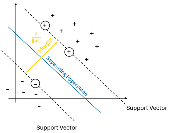
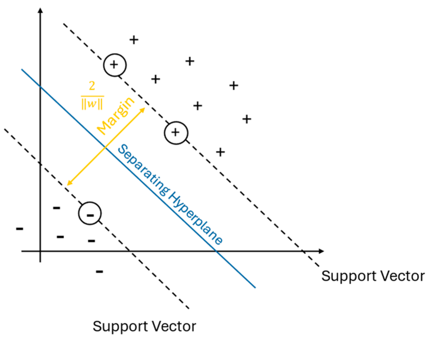
SVM has two categories: Support Vector Classification (SVC) and Support Vector Regression (SVR). The SVM is based on statistics produced by Vapnik (1963), which are supervised algorithms used in machine learning. Figure 2 shows an illustrative example of SVM. It identifies an optimal hyperplane that maximizes the margin between distinct categories in a high-dimensional feature space. This maximum-margin approach ensures robust classification boundaries. Furthermore, for regression tasks, the model executes linear regression within the high-dimensional vector space to predict continuous outcomes (Parray et al., 2020). To assess comparative efficacy, the SVC model is tested against the other selected classifiers within the study.

Figure 2. An illustration of a Support Vector Machine.

2.5.2. Random Forest (RF)

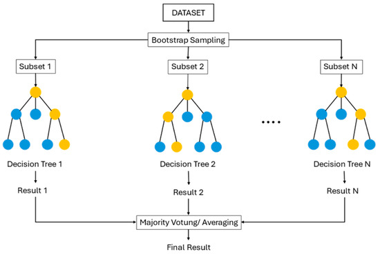
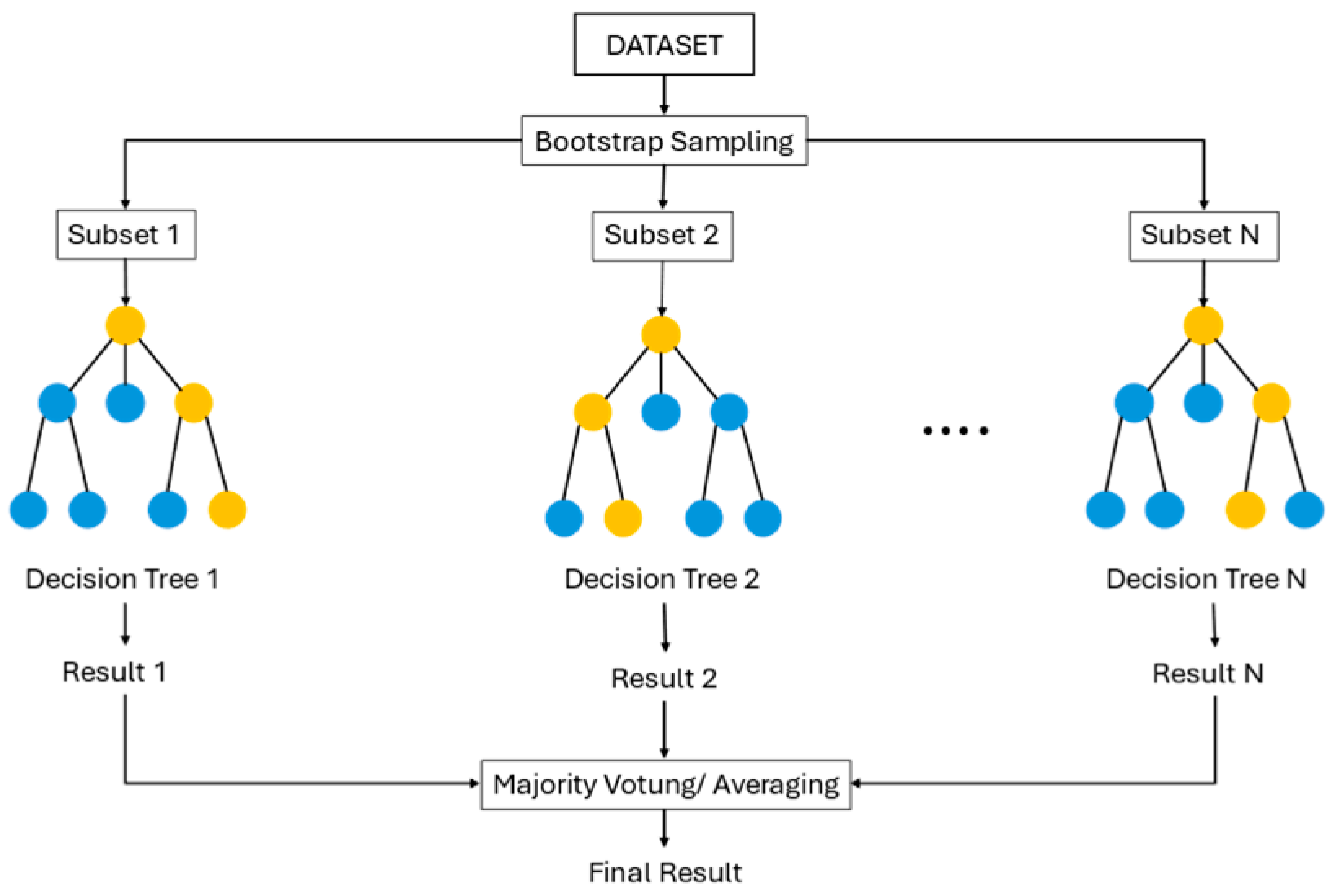
The Random Forest model, which is a representative ensemble learning method based on the decision tree model to gain more accuracy of prediction, was developed by Breiman (2001). The Random Forest (RF) functions as an ensemble of decision trees, utilizing an averaging mechanism to produce final predictions. The framework incorporates three distinct stochastic elements: bootstrap sampling for training data selection, the use of random feature subsets during node partitioning, and the restricted evaluation of feature subsets at each split point within the base learners. These features allow the RF to handle high-dimensional data without significant information loss, ultimately improving the model’s generalizability and accuracy (Chenyao, 2022; Nabipour et al., 2020). The processes are shown in Figure 3 and described in all the steps below:

Figure 3. An illustration of a Random Forest.

• Randomly sampling data subsets (Bootstrapping).
• Building a decision tree using standard decision tree algorithms for each bootstrap sample. At each split in the tree, we randomly select a subset of features.
• The tree will produce a prediction.
• Collection of all predictions and majority voting.

2.5.3. Extreme Gradient Boosting (XGBoost)

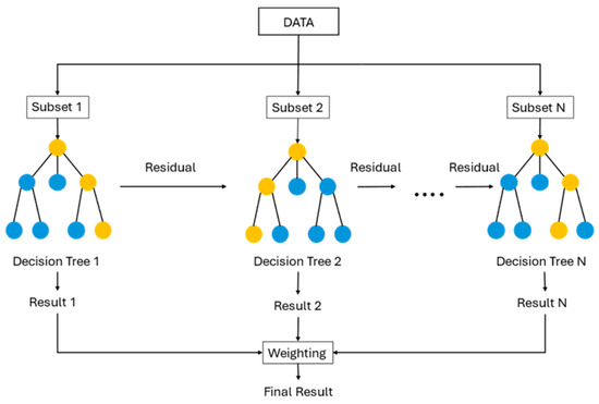
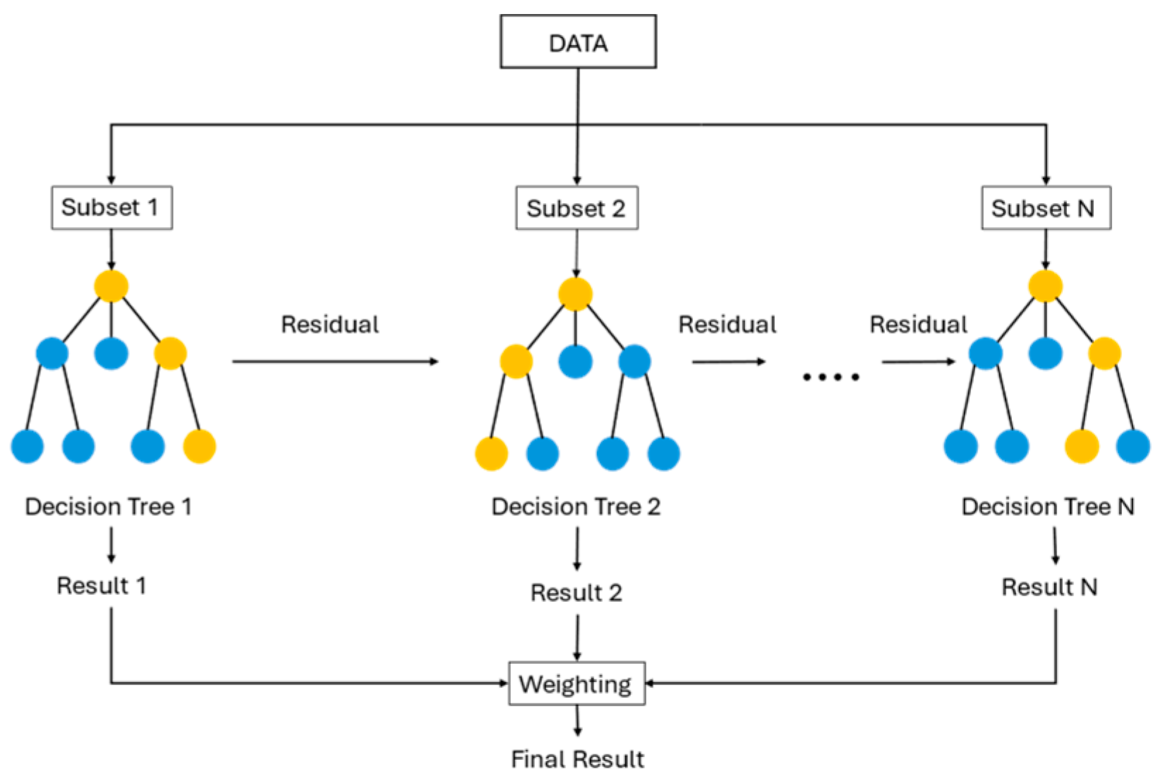
XGBoost, a powerful and widely employed machine learning approach, relies on the foundation of gradient boosting. XGBoost adopts an iterative approach to merge numerous weak learners, such as decision trees, into a strong prediction model. The algorithm’s more effective regularization techniques, in particular, assist in preventing overfitting, along with its ability to effectively handle missing values, making XGBoost a powerful instrument for predicting the stock market. Furthermore, XGBoost’s focus on minimizing prediction errors, as well as its ability to capture complex non-linear correlations in data, makes it better suited for accurately predicting index performance. These attributes determine XGBoost as a useful asset in constructing robust and reliable models for optimizing investment. Figure 4 depicts the process of the model.

Figure 4. An illustration of an Extreme Gradient Boosting.

The proposed predictive methodology consists of three distinct ML classifiers: RF, SVC, and XGBoost. These models are configured using the hyperparameters detailed in Table 4, using the input feature set specified in Table 3 to ensure data suitability for both the training and testing process. In time-series validation, we purge data between the training and testing sets to ensure that they are distinct. We embargo a specific window (10 days) after the test set to eliminate data leakage from serial correlation, and we utilize a walk-forward approach to train only past data to predict the future. For any given data in the test set, the model only uses the “Last two years” to learn and then makes a “Blind” prediction (out-of-sample prediction) for the “Next 3 Months”. This methodology addresses the non-stationary nature of financial data and prevents look-ahead bias and data leakage. Subsequently, the experimental design focuses on assessing the impact of MFI by comparing across two configurations—“withMFI” and “withoutMFI” feature sets in each ML over three stages: before, during, and after the COVID-19 pandemic.

The features are scaled by z-score normalization before being processed by the algorithm, which is vital for SVC. The standard scaler transforms the data such that each feature has a mean of 0 and a standard deviation of 1. The scaling is recalculated for each training fold individually. This prevents data leakage because the test data in the cross-validation is scaled using the mean and variance of the training data, rather than the whole dataset. The z-score is calculated as follows:

$$z={\displaystyle \frac{x-\mu }{\sigma }}$$

(15)

where z is the standardized value, x is the original feature value, μ is the mean of the feature across the training data, and σ is the standard deviation of the feature.

To handle class imbalance, particularly in the VN30 index, the experiment employs balanced class weights to penalize the misclassification of the minority class in SVC and RF. In addition, we implement a cost-sensitive learning approach via XGBoost’s parameter. By setting this ratio to the quotient of negative and positive samples, the model is penalized more heavily for misclassifying the minority trend, thereby enhancing the F1-score and preventing directional bias.

2.6. Portfolio Selection Model

This section first presents the Mean-Variance (MV) framework for portfolio optimization. Subsequently, we introduce an equally weighted (1/N) strategy as a robust benchmark to evaluate the performance of our proposed models. Finally, we provide a description of the experimental framework of asset allocation in a portfolio.

2.6.1. Mean-Variance Optimization Model (MV)

The Mean-Variance (MV) model was proposed by Markowitz (1952) to construct a stock portfolio from a variety of assets. In this model, investment return and risk are quantified by expected return and variance, respectively. The MV framework contributes to maximizing return and minimizing risk simultaneously. The Markowitz framework leverages raw datasets to determine the individual returns and volatilities of assets within a selection set. Extended versions of this model use the estimated prices to achieve maximum expected returns for a specific risk threshold or, alternatively, to minimize variance for a target return level (Kolm et al., 2014; Paiva et al., 2019). To map signals to returns, it is important to note that Mean-Variance optimizers require continuous expected returns, whereas machine learning models output binary signals. By calculating the historical averages of up days and down days, we bridge the gap between classification and portfolio theory. This provides the optimizer with a realistic reward estimate for each market’s signal. The procedure is formulated as follows:

$${\mu }_{i,t}=\left\{\begin{array}{c}{\overline{R}}_{i,up},if{s}_{i,t}=1\\ {\overline{R}}_{i,down},if{s}_{i,t}=0\end{array}\right.$$

(16)

where ${\mu }_{i,t}$ is the expected return for index $i$ at time $t$, $s_{i,t}$ ∈ {0,1} is the binary prediction from the model, ${\overline{R}}_{i,up}$ is the mean of historical positive returns, and ${\overline{R}}_{i,down}$ is the mean of historical negative returns.

In this context, standard deviation serves as the primary metric for assessing risk. Evidence from R. Huang et al. (2025) indicates that while crisis periods trigger a significant surge in portfolio-level risk, they do not result in a corresponding deterioration of overall investment yields, specifically aiming to optimize the portfolio to attain the maximum expected return relative to the portfolio’s variance. The primary objective of the MV portfolio in this research is to maximize the quadratic utility of the investor (Jana et al., 2009; Ledoit & Wolf, 2004; Yu et al., 2020), which is formulated as follows:

$$\underset{w_t}{\mathrm{m}\mathrm{a}\mathrm{x}}\underset{\mathrm{Expected}\mathrm{Return}}{\underbrace{w_t^T{\mathsf{\mu }}_t}}-\underset{\mathrm{Risk}\mathrm{Penalty}}{\underbrace{{\displaystyle \frac{\delta }{2}}{w}_t^T\mathsf{\Sigma }{w}_t}}\underset{\mathrm{L}2\mathrm{Regularization}}{-\underbrace{\mathsf{\gamma }{\left|\left|w_t\right|\right|}_2^2}}-\underset{\mathrm{Transaction}\mathrm{Cost}\mathrm{Penalty}}{\underbrace{\mathsf{\lambda }{\sum }_{i=1}^N\left|w_{i,t}-w_{i,t-1}\right|}}$$

(17)

where w is the weight vector, μ is the vector of expected returns, Σ is the covariance matrix, δ is the risk aversion coefficient, γ is the regularization parameter used to enforce diversification and weight stability, and λ represents the transaction cost (0.001). The final objective function is constructed by layering three distinct components: (1) the reward-risk tradeoff (Markowitz core), ensuring the portfolio stays on the best possible version of portfolio for every level of risk; (2) L2 regularization (Weight Smoothing), preventing the selection of extreme weights and encouraging stable diversification; and (3) a transaction cost penalty, which acts as a turnover control to prevent the optimizer from recommending excessive, costly trading.

The most significant departure from traditional Mean-Variance optimization in this study is the integration of directional signal constraints. The feasible range for each asset’s weight is dynamically adjusted based on the binary output of the machine learning classifier $\left({\mathrm{s}}_{\mathrm{i},\mathrm{t}}\in \left\{\mathrm{0,1}\right\}\right).$ The boundary condition for asset i at time t is formulated as

$$\left\{\begin{array}{ll}{w}_{\mathrm{i},\mathrm{t}}=0& \mathrm{if}{\mathrm{s}}_{\mathrm{i},\mathrm{t}}=0\left(\mathrm{Bearish}\mathrm{Signal}\right)\\ {0\le w}_{\mathrm{i},\mathrm{t}}\le w_{max}& \mathrm{if}{\mathrm{s}}_{\mathrm{i},\mathrm{t}}=1\left(\mathrm{Bullish}\mathrm{Signal}\right)\end{array}\right.$$

(18)

where $w_{max}$ represents the maximum allowable exposure to a single index (e.g., 0.45). This constraint effectively forces the optimizer to divest from an asset when a downtrend is predicted, thereby shifting the allocation to cash or the remaining bullish indices. This experiment allows for holding cash when market signals are predominantly bearish. Any residual weight is implicitly allocated to the risk-free cash component. This flexibility is critical during high-volatility regimes, such as the COVID-19 pandemic.

2.6.2. The Benchmark Model

As model uncertainty intensifies, generally we use a classical risk minimization framework to optimize decisions and tend to the uniform investment strategy when the market is ambiguous and equally weighted (1/N) as a protective “safety bubble” within a worst-case scenario (Pflug et al., 2012). Following the methodology of DeMiguel et al. (2009), we employ an equally weighted (1/N) portfolio as a benchmark to evaluate the performance of our proposed model. Their work demonstrated that none of the “sophisticated models” consistently yield a higher empirical evidence performance than an equally weighted (1/N) asset allocation.

In the asset allocation phase of this experiment, we evaluate the efficacy of the proposed frameworks—specifically the integration of three representative machine learning models (RF, SVC, and XGBoost) with MV optimization, which utilizes the “withMFI” dataset. These hybrid models are benchmarked against the naive 1/N strategy across three stages: before, during, and after the COVID-19 pandemic. To ensure a rigorous comparison, hyperparameters are held consistent with the proposed model architecture.

3. Experiments and Results

This section mentions the results of experiments in this study. It consists of (1) model accuracy measurement for each dataset using RF, SVC, and XGBoost, both with and without MFI, and (2) comparison of different portfolios using the MV and equally weighted (1/N) with different machine learning models with a transaction cost.

3.1. Results of Prediction

3.1.1. Accuracy on Dataset

The metrics are compared between two types of datasets that differ in their technical indicators: (1) WithoutMFI, including SMA, EMA, MACD, MOM, and RSI, and (2) WithMFI, including SMA, EMA, MACD, MOM, RSI, and the MFI signal. The three predictive models are tuned using optimal parameters across three different index markets (SET50, STI, and VN30). The dataset covers the period from February 2013 to December 2023. To evaluate the performance of the classification models, it is essential to utilize metrics that account for both the predictive power and the reliability of the signals. The foundation of all classification metrics is the Confusion Matrix, which categorizes the model’s predictions against the actual values. The components are as follows:

• True Positive (TP): Correctly predicted an upward move (1).
• True Negative (TN): Correctly predicted a downward mode (0).
• False Positive (FP): Predicted an upward move, but the market moved downward.
• False Negative (FN): Predicted a downward move, but the market moved upward.

Precision measures the reliability of the upward signals generated by the model, while recall assesses the model’s ability to identify all realized upward movements, as shown in Equations (19) and (20):

$$Precision={\displaystyle \frac{TP}{TP+FP}}$$

(19)

$$Recall={\displaystyle \frac{TP}{TP+FN}}$$

(20)

The F1-score is the harmonic mean of precision and recall, which is calculated using Equation (21):

$$F1=2·{\displaystyle \frac{Precision·Recall}{Precision+Recall}}$$

(21)

Finally, accuracy represents the proportion of total correct predictions from both upward and downward movements, formulated as follows:

$$Accuracy={\displaystyle \frac{TP+TN}{TP+TN+FP+FN}}$$

(22)

A detailed comparison of the classification metrics is presented in Table 5. Based on the experimental findings, the feature WithMFI resulted in improved accuracy, precision, recall, and F1-scores for all three models across all tested indices. In terms of classifiers, XGBoost is undoubtedly the top performer. When combined with MFI, it achieves remarkably high metrics: (1) SET50: Reaches an accuracy of 84.93%. (2) STI: Achieves an accuracy of 86.57% (3) VN30: Reaches a peak accuracy of 94.31% and an F1-score of 0.9484. While RF and SVC also show stable performance gains with the addition of MFI, their overall metrics remain lower than those of XGBoost. For example, in SET50, RF improves both accuracy (from 0.6340 to 0.6418) and F1-score (from 0.6271 to 0.6332). These results suggest that the gradient boosting framework of XGBoost is better suited for the high-frequency dynamics of financial data. Similarly, SVC has better performance when the MFI is added. This indicates that SVC requires high-quality features to define an effective decision hyperplane in noisy financial data.

Table 5. Performance according to dataset.

Index	Model	Dataset	Accuracy	Precision	Recall	F1-Score
SET50	RF	NO	0.6340	0.6526	0.6035	0.6271
		MFI	0.6418	0.6626	0.6063	0.6332
	SVC	NO	0.5370	0.5610	0.4230	0.4823
		MFI	0.5416	0.5699	0.4118	0.4782
	XGBoost	NO	0.7790	0.7991	0.7568	0.7774
		MFI	0.8493	0.8624	0.8383	0.8502
STI	RF	NO	0.6155	0.6312	0.5688	0.5984
		MFI	0.6276	0.6418	0.5893	0.6144
	SVC	NO	0.5387	0.5512	0.4517	0.4965
		MFI	0.6432	0.6627	0.5935	0.6262
	XGBoost	NO	0.7111	0.7097	0.7212	0.7154
		MFI	0.8657	0.8687	0.8638	0.8662
VN30	RF	NO	0.6101	0.6754	0.5788	0.6234
		MFI	0.6322	0.6754	0.6548	0.6649
	SVC	NO	0.5183	0.6217	0.3472	0.4455
		MFI	0.6361	0.6977	0.6126	0.6524
	XGBoost	NO	0.7332	0.7700	0.7435	0.7565
		MFI	0.9431	0.9595	0.9375	0.9484

Overall, when comparing predictive performance, the WithMFI dataset has the highest accuracy and F1-score across all three models. The consistent outperformance of the MFI-based feature engineering underscores the indicator’s importance for this experiment, as it directly correlates with the improved predictive accuracy observed across all ML classifiers.

3.1.2. Accuracy for Period

As shown previously, the MFI feature dominated across all datasets. To build upon these findings, this section analyzes the results across specific temporal intervals to evaluate model robustness under varying market conditions. By 2020, the COVID-19 pandemic had a significant impact on global stock markets, which amplified investor sentiment, fluctuations, and noise, ultimately affecting profitability (Li & Jiang, 2024). By partitioning the dataset into three distinct periods—before the COVID-19 pandemic (BEFORE), during the COVID-19 pandemic (COVID-19), and after the COVID-19 pandemic (AFTER)—we aim to showcase the versatility and predictive power of the MFI-integrated approach across diverse economic climates. The performance outcomes are summarized in Table 6, and the discussions are shown below.

Table 6. Performance according to period.

Metrics			Accuracy		Precision		Recall		F1-Score
Period	Index	Model	NO	MFI	NO	MFI	NO	MFI	NO	MFI
BEFORE	SET50	RF	0.6266	0.6328	0.6486	0.6595	0.5841	0.5785	0.6147	0.6164
		SVC	0.5155	0.5245	0.5381	0.5548	0.3518	0.3418	0.4254	0.4230
		XGBoost	0.7857	0.8550	0.8082	0.8731	0.7600	0.8374	0.7834	0.8549
	STI	RF	0.6208	0.6321	0.6339	0.6482	0.5635	0.5703	0.5966	0.6068
		SVC	0.5468	0.6343	0.5562	0.6552	0.4433	0.5601	0.4934	0.6039
		XGBoost	0.7111	0.8691	0.7161	0.8727	0.6950	0.8628	0.7054	0.8677
	VN30	RF	0.6088	0.6360	0.6833	0.6732	0.5259	0.6452	0.5944	0.6589
		SVC	0.5031	0.5964	0.5977	0.6658	0.2697	0.5207	0.3717	0.5844
		XGBoost	0.7275	0.9395	0.7829	0.9612	0.6919	0.9263	0.7346	0.9435
COVID-19	SET50	RF	0.6252	0.6444	0.6078	0.6242	0.7099	0.7290	0.6549	0.6725
		SVC	0.5602	0.5602	0.5510	0.5503	0.6603	0.6679	0.6007	0.6034
		XGBoost	0.7782	0.8470	0.7704	0.8346	0.7939	0.8664	0.7820	0.8502
	STI	RF	0.5966	0.6099	0.6125	0.6169	0.5547	0.6075	0.5822	0.6122
		SVC	0.4742	0.6616	0.4771	0.6606	0.3925	0.6830	0.4306	0.6716
		XGBoost	0.7170	0.8585	0.6983	0.8498	0.7774	0.8755	0.7357	0.8625
	VN30	RF	0.6291	0.6501	0.6818	0.6969	0.7453	0.7640	0.7122	0.7289
		SVC	0.5449	0.6902	0.6795	0.7410	0.4938	0.7640	0.5719	0.7523
		XGBoost	0.7572	0.9407	0.7586	0.9450	0.8882	0.9596	0.8183	0.9522
AFTER	SET50	RF	0.6680	0.6699	0.7343	0.7290	0.5651	0.5799	0.6387	0.6460
		SVC	0.5869	0.5811	0.6554	0.6605	0.4312	0.3978	0.5202	0.4965
		XGBoost	0.7568	0.8320	0.7992	0.8555	0.7100	0.8141	0.7520	0.8343
	STI	RF	0.6166	0.6301	0.6403	0.6477	0.6000	0.6333	0.6195	0.6404
		SVC	0.5761	0.6551	0.6042	0.6888	0.5370	0.6148	0.5686	0.6497
		XGBoost	0.7052	0.8613	0.7024	0.8750	0.7519	0.8556	0.7263	0.8652
	VN30	RF	0.5954	0.6012	0.6426	0.6529	0.5694	0.5623	0.6038	0.6042
		SVC	0.5434	0.7168	0.6068	0.7310	0.4448	0.7544	0.5133	0.7426
		XGBoost	0.7283	0.9576	0.7465	0.9709	0.7544	0.9502	0.7504	0.9604

• Before the COVID-19 period (2013–2019): Prior to the COVID-19 epidemic, the MFI demonstrated optimal performance. Specifically, XGBoost + withMFI achieved the highest accuracy and F1-score across all assets.
• COVID-19 period (2020–2021): During the pandemic, the MFI demonstrated outstanding performance, as indicated by the accuracy and F1-score in the table. Notably, the XGBoost + MFI framework maintained accuracy levels above 0.84 across all indices during the pandemic.
• After the COVID-19 period (2022–2023): After the pandemic, XGBoost continued to perform well across all studied markets. For instance, in the VN30 index, XGBoost + withMFI again achieved the highest accuracy (0.9576) and F1-score (0.9604). However, the MFI feature resulted in a slightly lower accuracy on the SET50 when paired with SVC.

Across the three analyzed periods—before the COVID-19 pandemic (BEFORE), during the COVID-19 pandemic (COVID-19), and after the COVID-19 pandemic (AFTER)—the integration of MFI with XGBoost consistently yields outstanding results, securing the highest predictive accuracy in nearly every scenario. A minor exception is observed in the VN30 index after the COVID-19 period, where SVC + withoutMFI achieves an accuracy of 58.69%. However, this result is only slightly higher than the 58.11% yielded by SVC + withMFI. This marginal difference falls within an acceptable range, and the MFI-augmented models remain highly competitive. Overall, it is noted that the MFI effectively captures market movements even under abnormal conditions, validating its reliability as a sentiment indicator in both stable and highly volatile market conditions.

The prediction performance of the two competing feature sets (feature without MFI and with MFI) is compared using the Diebold–Mariano Test (DM test) (Mohana, 2020). The results in Table 7 reveal that the inclusion of the MFI signal significantly reduces prediction errors in six out of the nine observed cases (p < 0.05). The positive DM statistics across all rows suggest that models incorporating the MFI signal consistently achieve lower prediction errors than the baseline. Notably, in the VN30 index, the MFI signal is universally significant across all algorithms (p < 0.01), with XGBoost achieving an exceptionally high DM statistic of 25.919, effectively mitigating the noise inherent in price-only indicators.

Table 7. Significance test of MFI.

Index	Model	Comparison	DM_Stat	p-Value	Significant
SET50	RF	NO MFI vs. MFI	1.2499	0.2115	No
	SVC	NO MFI vs. MFI	0.7372	0.4610	No
	XGB	NO MFI vs. MFI	8.872	<0.001	Yes
STI	RF	NO MFI vs. MFI	1.7544	0.0795	No
	SVC	NO MFI vs. MFI	10.0412	<0.001	Yes
	XGB	NO MFI vs. MFI	19.2291	<0.001	Yes
VN30	RF	NO MFI vs. MFI	3.0448	0.0023	Yes
	SVC	NO MFI vs. MFI	11.1075	<0.001	Yes
	XGB	NO MFI vs. MFI	25.919	<0.001	Yes

Across all three indices, the XGBoost classifier benefited significantly from the addition of the MFI signal. Even in the SET50 index, where RF and SVC failed to reach significance, XGBoost remained highly significant (p < 0.001).

The results in Table 8 present the observed accuracy differentials between the competing algorithms using the DM test. The values of the DM test are all highly negative and exceptionally strong, indicating that the probability of these models performing equally is virtually zero. This confirms that the prediction error of XGBoost is significantly lower than that of RF or SVC. XGBoost consistently takes the first-place position, and the DM test confirms that its predictive performance is significantly better than both other models in every single scenario. The p-values of <0.001 show that the results are significant at the 99.9% confidence level. This allows us to reject the null hypothesis of equal prediction accuracy. The magnitude of these statistics suggests that the XGBoost framework provides a structurally superior mapping of the complex, non-linear feature interactions in equity data compared to the Random Forest and Support Vector Machine alternatives.

Table 8. Significance test of model.

Index	Model	Comparison	DM_Stat	p-Value	Significant
SET50	XGB	vs. RF	−22.6922	<0.001	Yes
SET50	XGB	vs. SVC	−28.7837	<0.001	Yes
STI	XGB	vs. SVC	−22.8306	<0.001	Yes
STI	XGB	vs. RF	−26.0498	<0.001	Yes
VN30	XGB	vs. SVC	−33.0448	<0.001	Yes
VN30	XGB	vs. RF	−34.1165	<0.001	Yes

3.2. Results of Optimal Portfolio

After the classification results are generated, the next step is to turn those predictive signals into an actionable investment strategy aimed at maximizing returns. To construct the portfolio, we evaluate two distinct methods: the Mean-Variance (MV) optimization and the naïve 1/N baseline. The trading system is driven by the predictive signals from the MFI-enhanced classifier. The overall efficacy of these strategies is then measured using cumulative returns, maximum drawdown, risk-adjusted return and the Sharpe ratio.

To quantify the risk-return profile of the MV and 1/N strategies, the following financial metrics are utilized:

• Sharpe Ratio (S): It is the primary metric for assessing risk-adjusted efficiency, measuring the excess return per unit of volatility. The equation is as follows:

$$S={\displaystyle \frac{{\mathsf{\mu }}_p-r_f}{{\mathsf{\sigma }}_p}}$$

(23)

where ${\mu }_p$ is the annualized portfolio return, $r_f$ is the risk-free rate, and ${\sigma }_p$ is the annualized standard deviation of returns.

2.

Maximum Drawdown (MDD): This is a critical metric for understanding the worst-case scenario, representing the largest peak-to-trough decline in the value of the portfolio. The equation is as follows:

$$MDD=\min \left({\displaystyle \frac{V_t-{\mathrm{Peak}}_t}{{\mathrm{Peak}}_t}}\right)$$

(24)

where $V_t$ is the portfolio value at time t, and ${Peak}_t$ is the maximum value reached before time t.

3.

Risk-Adjusted Return (RAR): This is defined as the ratio of annualized return to the absolute maximum drawdown. The equation is as follows:

$$RAR={\displaystyle \frac{\mathrm{Annualized}\mathrm{Return}}{\left|MDD\right|}}$$

(25)

After evaluating the performance of the portfolio to confirm that the MV truly outperforms the 1/N benchmark, we utilize the Ledoit and Wolf (2007) test. This method is specifically designed for Sharpe ratios. We incorporate Heteroskedasticity and Autocorrelation Consistent (HAC) standard errors. This adjustment ensures that the p-values are not biased by the noise in the data. This is essential for financial time series because market returns often exhibit (1) volatility clustering (heteroskedasticity) and (2) serial autocorrelation.

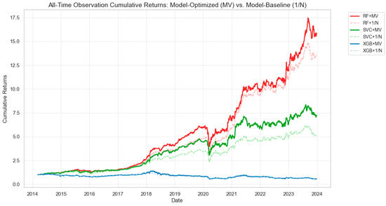
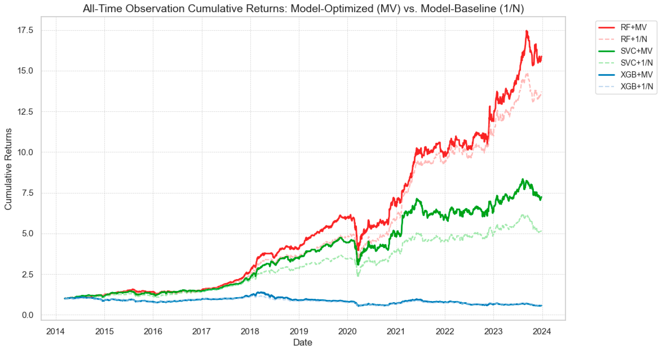
As illustrated in Figure 5, the cumulative returns of each portfolio strategy with transaction costs are analyzed throughout the entire experimental range using the MFI-enhanced classifiers. The results are visualized in a line graph. The Y-axis tracks the cumulative return, and the X-axis identifies the observation years. The graph trend of RF + MV is upwardly different from the blueline of XGBoost + MV, which is lower and slightly downward.

Figure 5. Cumulative returns of portfolios.

The results from Table 9 are as follows: RF + MV leads the group with the highest return of 14.88. However, its Sharpe ratio is slightly lower than the benchmark. The RF + MV strategy generates wealth up to 216% higher than the benchmark throughout the entire period, which provides substantial benefits for investors, even with slightly higher daily volatility. For SVC, it shows the most consistent improvement through optimization. The MV strategy outperforms the benchmark in Sharpe ratio, cumulative returns, RAR, and MDD. This shows that MV combined with ML can indeed overcome the limitations of the 1/N strategy in terms of both return and risk. Surprisingly, the XGBoost portfolios resulted in negative cumulative returns and Sharpe ratios despite their high predictive accuracy. This likely stems from “Signal Flickering.” If the XGBoost model flips its signal too often (even if the directions are correct), the 0.1% transaction cost erodes the capital base faster than the model can capture gains.

Table 9. Performance of portfolio.

Model	Strategy	Sharpe	RAR	MDD	Cumulative Return	p-Value	Significant
RF	MV	1.7080	0.8049	−0.3563	14.8800	0.3859	No
	1/N	1.8257	0.8466	−0.3178	12.7162	-	-
SVC	MV	1.1894	0.5963	−0.3539	6.2431	0.5477	No
	1/N	1.1148	0.4756	−0.3668	4.1787	-	-
XGBoost	MV	−0.2211	−0.0639	−0.6186	−0.4314	0.6745	No
	1/N	−0.2826	−0.0722	−0.5669	−0.4071	-	-

A critical finding is that although the RF + MV strategy generated more wealth than the RF + 1/N benchmark, the p-value (0.3859) indicates that the result is not statistically significant. The fact that the p-value of the Ledoit–Wolf test did not show a significant difference (p > 0.05) does not mean that the MV strategy has failed. Rather, it is due to the high correlation structure of daily returns, as both the MV and 1/N strategies are filtered from the same machine learning (signal-filtered universe), resulting in both portfolios trading in the same direction for many days. However, considering economic significance, the MV strategy clearly demonstrated its superiority, generating a cumulative return that is 206% higher than 1/N in the SVC model and 216% higher in the RF model. This confirms that Mean-Variance weighting combined with dynamic bounds can create tangible long-term value.

As shown previously, the results from the all-time experiments indicate that the MV strategy provides a better cumulative return. These overarching results are further detailed in Table 10, which partitions the performance into three distinct temporal regimes: the period before COVID-19 (“BEFORE”), during COVID-19 (“COVID-19”), and after COVID-19 (“AFTER”).

Table 10. Performance of portfolios over time.

Period	Model	Portfolio	Sharpe	RAR	MDD	Cumulative Return
BEFORE	RF	MV	2.4279	1.7900	−0.1720	5.0713
		1/N	2.2088	1.4234	−0.1794	3.4638
	SVC	MV	1.5740	0.9646	−0.2159	2.3211
		1/N	1.5386	0.8492	−0.2181	1.9176
	XGBoost	MV	−0.3050	−0.0979	−0.4411	−0.2744
		1/N	−0.6147	−0.1829	−0.3845	−0.3705
COVID-19	RF	MV	1.5843	1.2018	−0.3443	1.1955
		1/N	1.7146	1.2153	−0.3212	1.1273
	SVC	MV	0.2964	0.2379	−0.3339	0.0936
		1/N	0.4473	0.3071	−0.3380	0.1720
	XGBoost	MV	0.3488	0.2450	−0.3511	0.1211
		1/N	0.4420	0.2858	−0.3300	0.1592
AFTER	RF	MV	1.7808	1.8696	−0.1465	0.7132
		1/N	1.8130	2.1805	−0.1083	0.5966
	SVC	MV	0.3866	0.4147	−0.1709	0.1174
		1/N	0.3383	0.3045	−0.1719	0.0865
	XGBoost	MV	−0.4959	−0.3141	−0.2970	−0.2041
		1/N	−0.5870	−0.3269	−0.2368	−0.1623

Before the COVID-19 pandemic (2013–2019), the MV strategy yielded superior returns compared to the 1/N benchmark across all metrics. The RF + MV portfolio achieves a Sharpe ratio as high as 2.4279 and a cumulative return of 5.0713 (or 507%), decisively outperforming 1/N. This proves that the bagging mechanism of RF is highly resistant to noise and better captures long-term trend signals. The dataset for this period is marked by various events and crises that contribute to extreme market volatility (Nguyen et al., 2022; Saetia & Yokrattanasak, 2023), making it difficult to accurately capture price movements.

During the COVID-19 pandemic, market volatility went up dramatically, and the correlation of all equities converged to 1 (meaning they fell together). This causes the MV strategy, which relies on historical covariance data, to suffer from severe estimation errors. In contrast, the 1/N strategy, which divides weights equally regardless of historical data, proves far more robust. As a result, the overall performance of the MV portfolio is lower than the benchmark. However, the RF + MV still has a higher cumulative return than the 1/N, despite a slightly lower Sharpe ratio. In terms of economic significance, the optimized MV strategy still generates more revenue even during a crisis.

As the market emerges from the COVID-19 crisis and enters the “AFTER” phase, market volatility begins to return to normal conditions. The results indicate that the MV strategy begins to perform well again. Specifically, the RF + MV gained a higher cumulative return (0.7132) than 1/N (0.5966). For the SVC model, the MV strategy recovers its advantage over 1/N across all metrics. However, for the RF model, the 1/N benchmark maintained a better RAR and MDD compared to MV.

Overall, the empirical results clearly confirm that the RF model is the champion of this study, regardless of market conditions. The MV strategy shows its true potential in trending or normal markets because it can use the covariance matrix to accurately avoid risk. Ultimately, these findings highlight that no single strategy is a winner in all market conditions. The 1/N benchmark serves as a safeguard during crises. However, the MV strategy incorporating ML (especially the RF model) acts as the most powerful wealth generator in the long term.

4. Conclusions

This study presented the integration of stock movement forecasting with quantitative portfolio optimization. The objectives of this research were: (1) to identify key technical factors influencing market movements, with a particular emphasis on the application of the Money Flow Index (MFI) and explore relevant optimization strategies; (2) to evaluate the accuracy of selected predictive models, including RF, SVC, and XGBoost, across three prominent Southeast Asian indices, the SET50, STI, and VN30; and (3) to construct optimal trading strategies by conducting a comparative analysis between the MV and 1/N allocation strategies, ultimately identifying the most effective approach.

In the first part of this study, we involved predictive modeling for three prominent market indices in Southeast Asia (SEA): the SET50, STI, and VN30. Central to this analysis was the evaluation of the MFI as a proxy for the measurement of psychological market (Phuong, 2021). To isolate its impact, we benchmarked a baseline feature set (“withoutMFI”) against an MFI-integrated configuration (“withMFI”) across various hyperparameter-tuned environments. Utilizing three core classifiers—Random Forest (RF), Support Vector Classifier (SVC), and Extreme Gradient Boosting (XGBoost)—the empirical results across the entire experimental range clearly demonstrate that MFI integration significantly enhances predictive performance. The following configurations emerged as superior:

• SET50: The XGBoost model with MFI achieved an accuracy of 84.93%.
• STI: The XGBoost model with MFI led with an accuracy of 86.57%.
• VN30: The XGBoost model with MFI yielded a peak of 94.31%.

To further validate the robustness of this MFI-enhanced approach, we assessed model performance under periods of extreme market stress. By dividing the dataset into three distinct intervals—BEFORE (before the COVID-19 pandemic), COVID-19 (during the COVID-19 pandemic), and AFTER (after the COVID-19 pandemic)—we tested the models against heightened volatility and market noise. The findings confirm that MFI-enhanced classifiers, particularly those leveraging the XGBoost architectures, maintain high predictive accuracy and consistency across all markets. Their resilience during these timeframes underscores the efficacy of the proposed methodology, especially in abnormal market conditions.

Secondly, we combined the MFI-enhanced classifiers with two different portfolio optimization frameworks (with 0.1% transaction cost): the Mean-Variance (MV) model and the naïve 1/N benchmark. An analysis of all metrics across the entire experimental timeframe indicated that the RF + MV configuration achieved the most cumulative return with a slightly higher risk. To further validate the robustness of the proposed methodology, the experiment was split into three distinct intervals: BEFORE, COVID-19, and AFTER. The results show that the RF model outperforms, regardless of market conditions. These findings highlight that no single strategy is a winner in all market conditions, and the 1/N benchmark serves as a safeguard during crises.

Finally, the results from the prediction method demonstrated that the MFI plays a significant role in the feature set of input and revealed that XGBoost has superior performance.

Even though the proof has been shown in evidence, the study still has several limitations:

• This study focused only on three index markets in Southeast Asia, consisting of SET50, STI, and VN30. Thus, the insights obtained from this study might not be practical for other assets.
• This study only used a set of technical indicators to estimate the direction of the index, but it can additionally utilize economic indicators.
• Several factors affect market indices and can serve as additional inputs to improve performance. These factors include legal risks, political issues, interest rates, and the impact of the COVID-19 pandemic.
• We utilize only the Markowitz Mean-Variance approach to optimize the trading portfolio. In addition, the incorporation of a stop-loss mechanism can enhance profitability.

To build upon this work, future research should explore the inclusion of individual stocks and a more diverse range of asset classes within the trading portfolio. Furthermore, performance can be improved by adding a stop-loss mechanism. Additionally, it should integrate economic indicators alongside technical indicators and consider text data from various sources to manage periods of fluctuation much more effectively.

References

- A Ilemobayo, J., Durodola, O., Alade, O., Awotunde, O. J., Olanrewaju, A. T., Falana, O., Ogungbire, A., Osinuga, A., Ogunbiyi, D., Ifeanyi, A., Odezuligbo, I. E., & Edu., O. E. (2024). Hyperparameter tuning in machine learning: A comprehensive review. Journal of Engineering Research and Reports, 26(6), 388–395. [Google Scholar] [CrossRef] [Scilit]
- Asad, M. (2015, October 14–16). Optimized stock market prediction using ensemble learning. 2015 9th International Conference on Application of Information and Communication Technologies (AICT), Rostov on Don, Russia. [Google Scholar]
- Ayala, J., García-Torres, M., Noguera, J. L. V., Gómez-Vela, F., & Divina, F. (2021). Technical analysis strategy optimization using a machine learning approach in stock market indices. Knowledge-Based Systems, 225, 107119. [Google Scholar] [CrossRef] [Scilit]
- Basak, S., Kar, S., Saha, S., Khaidem, L., & Dey, S. R. (2019). Predicting the direction of stock market prices using tree-based classifiers. The North American Journal of Economics and Finance, 47, 552–567. [Google Scholar] [CrossRef] [Scilit]
- Bernard, V. L., & Thomas, J. K. (1990). Evidence that stock prices do not fully reflect the implications of current earnings for future earnings. Journal of Accounting and Economics, 13, 305–340. [Google Scholar] [CrossRef] [Scilit]
- Breiman, L. (2001). Random forests. Machine Learning, 45, 5–32. [Google Scholar] [CrossRef] [Scilit]
- Bustos, O., & Pomares-Quimbaya, A. (2020). Stock market movement forecast: A Systematic review. Expert Systems with Applications, 156, 113464. [Google Scholar] [CrossRef] [Scilit]
- Chaengkham, S., & Wianwiwat, S. (2021). Stock market index prediction using machine learning: Evidence from leading Southeast Asian. Thailand and The World Economy, 39(2), 56–64. [Google Scholar]
- Chaweewanchon, A., & Chaysiri, R. (2022). Markowitz mean-variance portfolio optimization with predictive stock selection using machine learning. International Journal of Financial Studies, 10, 64. [Google Scholar] [CrossRef] [Scilit]
- Chen, H., Chong, T. T.-L., & Duan, X. (2010). A principal-component approach to measuring investor sentiment. Quantitative Finance, 10(4), 339–347. [Google Scholar] [CrossRef] [Scilit]
- Chenyao, M. (2022, April 15–17). Stock selection model based on random forest. 2022 International Conference on Artificial Intelligence, Internet and Digital Economy (ICAID 2022), Shenzhen, China. [Google Scholar]
- da Costa, T. R. C. C., Nazário, R. T., Bergo, G. S. Z., Sobreiro, V. A., & Kimura, H. (2015). Trading system based on the use of technical analysis: A computational experiment. Journal of Behavioral and Experimental Finance, 6, 42–55. [Google Scholar] [CrossRef] [Scilit]
- DeMiguel, V., Garlappi, L., & Uppal, R. (2009). Optimal versus naive diversification: How inefficient is the 1/N portfolio strategy? The Review of Financial Studies, 22(5), 1915–1953. [Google Scholar] [CrossRef] [Scilit]
- Dev, D., & Bhatnagar, V. (2024). Hybrid RFSVM: Hybridization of SVM and random forest models for detection of fake news. Algorithms, 17, 459. [Google Scholar] [CrossRef] [Scilit]
- Dongrey, S. (2022). Study of market indicators used for technical. International Journal of Engineering and Management Research, 12(2), 64–83. [Google Scholar] [CrossRef] [Scilit]
- Ferreira, F., Gandomi, A., & Cardoso, R. (2021). Artificial intelligence applied to stock market trading: A review. IEEE Access, 9, 30898–30917. [Google Scholar] [CrossRef] [Scilit]
- Fonou-Dombeu, N. C., Nomlala, B. C., & Nyide, C. J. (2024). Investigating the effect of investor sentiment on stock return sensitivity to fundamental factors: Case of JSE listed companies. Cogent Business & Management, 11(1), 2353846. [Google Scholar] [CrossRef] [Scilit]
- Fredrik, L. (2007). Automatic stock market trading based on technical analysis [Master’s thesis, Norwegian University of Science and Technology]. [Google Scholar]
- Gao, Y., Zhao, C., Sun, B., & Zhao, W. (2022). Effects of investor sentiment on stock volatility: New evidences from multi-source data in China’s green stock markets. Financial Innovation, 8(1), 77. [Google Scholar] [CrossRef] [Scilit] [PubMed]
- Gorenc Novak, M., & Velušček, D. (2016). Prediction of stock price movement based on daily high prices. Quantitative Finance, 16(5), 793–826. [Google Scholar] [CrossRef] [Scilit]
- Huang, M., Dang, S., & Bhuiyan, M. A. (2026). Multi-objective portfolio optimization for stock return prediction using machine learning. Expert Systems with Applications, 298, 129672. [Google Scholar] [CrossRef] [Scilit]
- Huang, R., Kambouroudis, D., & McMillan, D. G. (2025). Is portfolio diversification still effective: Evidence spanning three crises from the perspective of U.S. investors. Journal of Asset Management, 26(2), 115–135. [Google Scholar] [CrossRef] [Scilit]
- Ismail, M. S., Md Noorani, M. S., Ismail, M., Abdul Razak, F., & Alias, M. A. (2020). Predicting next day direction of stock price movement using machine learning methods with persistent homology: Evidence from Kuala Lumpur Stock Exchange. Applied Soft Computing, 93, 106422. [Google Scholar] [CrossRef] [Scilit]
- Jana, P., Roy, T. K., & Mazumder, S. K. (2009). Multi-objective possibilistic model for portfolio selection with transaction cost. Journal of Computational and Applied Mathematics, 228(1), 188–196. [Google Scholar] [CrossRef] [Scilit]
- Kocaoğlu, D., Turgut, K., & Konyar, M. Z. (2022). Sector-based stock price prediction with machine learning models. Sakarya University Journal of Computer and Information Sciences, 5(3), 415–426. [Google Scholar] [CrossRef] [Scilit]
- Kolm, P. N., Tütüncü, R., & Fabozzi, F. J. (2014). 60 Years of portfolio optimization: Practical challenges and current trends. European Journal of Operational Research, 234(2), 356–371. [Google Scholar] [CrossRef] [Scilit]
- Kumari, J., & Mahakud, J. (2016). Investor sentiment and stock market volatility: Evidence from India. Journal of Asia-Pacific Business, 17(2), 173–202. [Google Scholar] [CrossRef] [Scilit]
- Kumbure, M. M., Lohrmann, C., Luukka, P., & Porras, J. (2022). Machine learning techniques and data for stock market forecasting: A literature review. Expert Systems with Applications, 197, 116659. [Google Scholar] [CrossRef] [Scilit]
- Ledoit, O., & Wolf, M. (2004). A well-conditioned estimator for large-dimensional covariance matrices. Journal of Multivariate Analysis, 88(2), 365–411. [Google Scholar] [CrossRef] [Scilit]
- Ledoit, O., & Wolf, M. (2007). Robust performance hypothesis tests with the sharpe ratio. Journal of Empirical Finance, 15, 850–859. [Google Scholar] [CrossRef] [Scilit]
- Lee, W. Y., Jiang, C. X., & Indro, D. C. (2002). Stock market volatility, excess returns, and the role of investor sentiment. Journal of Banking & Finance, 26(12), 2277–2299. [Google Scholar] [CrossRef] [Scilit]
- Li, K., & Jiang, X. (2024). China’s stock market under COVID-19: From the perspective of behavioral finance. International Journal of Financial Studies, 12(3), 70. [Google Scholar] [CrossRef] [Scilit]
- Ma, Y., Han, R., & Wang, W. (2021). Portfolio optimization with return prediction using deep learning and machine learning. Expert Systems with Applications, 165, 113973. [Google Scholar] [CrossRef] [Scilit]
- Marek, P., & Marková, V. (2020, February 4–6). Optimization and testing of money flow index. 2020 19th Conference on Applied Mathematics (APLIMAT 2020), Bratislava, Slovakia. [Google Scholar]
- Markowitz, H. (1952). Portfolio selection. The Journal of Finance, 7(1), 77–91. [Google Scholar] [CrossRef] [Scilit]
- Misra, P., & Chaurasia, S. (2020). Data-driven trend forecasting in stock market using machine learning techniques. Journal of Information Technology Research, 13(1), 130–149. [Google Scholar] [CrossRef] [Scilit]
- Mohana, F. (2020). Applying diebold–Mariano test for performance evaluation between individual and hybrid time-series models for modeling bivariate time-series data and forecasting the unemployment rate in the USA. Springer. [Google Scholar]
- Mokhtari, S., Yen, K. K., & Liu, J. (2021). Effectiveness of artificial intelligence in stock market prediction based on machine learning. International Journal of Computer Applications, 183(7), 1–8. [Google Scholar] [CrossRef] [Scilit]
- Moodley, F., Ferreira-Schenk, S., & Matlhaku, K. (2024). Effect of market-wide investor sentiment on South African government bond indices of varying maturities under changing market conditions. Economies, 12(10), 265. [Google Scholar] [CrossRef] [Scilit]
- Nabipour, M., Nayyeri, P., Jabani, H., S, S., & Mosavi, A. (2020). Predicting stock market trends using machine learning and deep learning algorithms via continuous and binary data; a comparative analysis. IEEE Access, 8, 150199–150212. [Google Scholar] [CrossRef] [Scilit]
- Narayanasamy, A., Panta, H., & Agarwal, R. (2023). Relations among bitcoin futures, bitcoin spot, investor attention, and sentiment. Journal of Risk and Financial Management, 16(11), 474. [Google Scholar] [CrossRef] [Scilit]
- Nguyen, T. C., Castro, V., & Wood, J. (2022). A new comprehensive database of financial crises: Identification, frequency, and duration. Economic Modelling, 108, 105770. [Google Scholar] [CrossRef] [Scilit]
- Paiva, F. D., Cardoso, R. T. N., Hanaoka, G. P., & Duarte, W. M. (2019). Decision-making for financial trading: A fusion approach of machine learning and portfolio selection. Expert Systems with Applications, 115, 635–655. [Google Scholar] [CrossRef] [Scilit]
- Parray, I. R., Khurana, S. S., Kumar, M., & Altalbe, A. A. (2020). Time series data analysis of stock price movement using machine learning techniques. Soft Computing, 24(21), 16509–16517. [Google Scholar] [CrossRef] [Scilit]
- Pflug, G. C., Pichler, A., & Wozabal, D. (2012). The 1/N investment strategy is optimal under high model ambiguity. Journal of Banking & Finance, 36(2), 410–417. [Google Scholar] [CrossRef] [Scilit]
- Ph, H., & Rishad, A. (2020). An empirical examination of investor sentiment and stock market volatility: Evidence from India. Financial Innovation, 6(1), 34. [Google Scholar] [CrossRef] [Scilit]
- Phuoc, T., Anh, P. T. K., Tam, P. H., & Nguyen, C. V. (2024). Applying machine learning algorithms to predict the stock price trend in the stock market—The case of Vietnam. Humanities and Social Sciences Communications, 11(1), 393. [Google Scholar] [CrossRef] [Scilit]
- Phuong, L. C. M. (2021). Investor sentiment by money flow index and stock return. International Journal of Financial Research, 12(4), 33–42. [Google Scholar] [CrossRef] [Scilit]
- Prashanth, G., VSSKR Naganjaneyulu, G., Revanth, M., & Narasimhadhan, A. V. (2023). Multi indicator based hierarchical strategies for technical analysis of crypto market paradigm. International Journal of Electrical and Computer Engineering Systems, 14(7), 765–780. [Google Scholar] [CrossRef] [Scilit]
- QuantifiedTrading. (2025). 25 factors that influence stock market prices. Available online: https://www.quantifiedstrategies.com/stock-market-price-factors/ (accessed on 31 January 2025).
- Quong, G. S., & Soudack, A. (1989). Volume-weighted RSI: Money flow. Technical Analysis of Stocks and Commodities, 7(3), 76–77. [Google Scholar]
- Rai, B., & Soltanisehat, L. (2025). A multi-model machine learning framework for daily stock price prediction. Big Data and Cognitive Computing, 9(10), 248. [Google Scholar] [CrossRef] [Scilit]
- Saetia, K., & Yokrattanasak, J. (2023). Stock movement prediction using machine learning based on technical indicators and Google trend searches in Thailand. International Journal of Financial Studies, 11(1), 5. [Google Scholar] [CrossRef] [Scilit]
- Sangsawai, N., & Sutivong, D. (2023). Analyzing impact of economic indicators on Vietnam stock market using machine learning techniques. Industrial Engineering and Applications, 35, 279–288. [Google Scholar] [CrossRef] [Scilit]
- Steven, B. A. (2000). Technical analysis from A to Z (2nd ed.). McGraw-Hill. [Google Scholar]
- Vapnik, V. N. (1963). Pattern recognition using generalized portrait method. Automation and Remote Control, 24, 774–780. [Google Scholar]
- Wang, S. (2020, February 14–16). The prediction of stock index movements based on machine learning. 2020 12th International Conference on Computer and Automation Engineering, Sydney, NSW, Australia. [Google Scholar]
- Wang, W., Li, W., Zhang, N., & Liu, K. (2020). Portfolio formation with preselection using deep learning from long-term financial data. Expert Systems with Applications, 143, 113042. [Google Scholar] [CrossRef] [Scilit]
- Worasucheep, C. (2022). Ensemble classifier for stock trading recommendation. Applied Artificial Intelligence, 36(1), 2001178. [Google Scholar] [CrossRef] [Scilit]
- Ye, C., Qiu, Y., Lu, G., & Hou, Y. (2018). Quantitative strategy for the Chinese commodity futures market based on a dynamic weighted money flow model. Physica A: Statistical Mechanics and its Applications, 512, 1009–1018. [Google Scholar] [CrossRef] [Scilit]
- Yu, J.-R., Paul Chiou, W.-J., Lee, W.-Y., & Lin, S.-J. (2020). Portfolio models with return forecasting and transaction costs. International Review of Economics & Finance, 66, 118–130. [Google Scholar] [CrossRef] [Scilit]
- Yuan, X., Yuan, J., Jiang, T., & Ain, Q. U. (2020). Integrated long-term stock selection models based on feature selection and machine learning algorithms for China stock market. IEEE Access, 8, 22672–22685. [Google Scholar] [CrossRef] [Scilit]
Disclaimer/Publisher’s Note: The statements, opinions and data contained in all publications are solely those of the individual author(s) and contributor(s) and not of MDPI and/or the editor(s). MDPI and/or the editor(s) disclaim responsibility for any injury to people or property resulting from any ideas, methods, instructions or products referred to in the content. |
© 2026 by the authors. Licensee MDPI, Basel, Switzerland. This article is an open access article distributed under the terms and conditions of the Creative Commons Attribution (CC BY) license.