


Abstract
The quality of governance is a key driver of resource mobilisation in a context marked by successive shocks that exacerbate fiscal imbalances. This study aims to analyse the role of institutional quality in the relationship between public expenditure and tax revenue in a panel of 162 countries, broken down into developed and emerging economies between 2000 and 2023. Using causality tests and the cross-sectional autoregressive model with staggered lags (CS-ARDL) to control for cross-sectional heterogeneity and cross-dependence, the results reveal a bidirectional causality linking expenditure and revenue for the entire panel; emerging countries are more sensitive to fiscal policies; public expenditure significantly stimulates tax revenue in the short and long term, with an effect amplified by institutional quality; long-term sustainability depends crucially on the institutional framework. This study highlights the need for targeted institutional reforms and fiscal rules differentiated according to countries’ level of economic development.
1. Introduction
Since the early 2020s, global economies have been facing a series of global shocks of exceptional magnitude, putting a strain on the fiscal stability of states. The COVID-19 health crisis has severely disrupted macroeconomic balances, forcing states to resort to massive fiscal support measures in the face of the collapse of economic activity. Just as economies were beginning to recover, the Russia–Ukraine conflict reignited geopolitical tensions, exacerbating volatility in the energy and food markets and increasing fiscal burdens through higher public spending. At the same time, growing economic rivalry between the United States and China has resulted in a persistent trade war, fueling instability in global trade and complicating fiscal planning in many exporting countries. Added to this is instability in the Middle East, whose economic repercussions, although indirect, are not insignificant, particularly for developing countries.
In this global context marked by recurring shocks and growing pressure on public finances, the issue of fiscal sustainability becomes crucial. It depends fundamentally on the ability of governments to effectively mobilize their domestic resources while controlling spending dynamics. However, this ability varies greatly depending on the level of economic development and the quality of public institutions. The differences observed between developed and emerging countries highlight the diverse challenges facing economic policymakers. Therefore, understanding the relationship between public spending, tax revenues, and institutional quality is an important issue for fiscal sustainability, particularly in a global context marked by recurring shocks and growing pressure on public finances (Baharumshah et al., 2016).
In the period leading up to COVID-19, several developing countries took on massive debt, both on international financial markets and from bilateral creditors, notably China. According to Estevao and Essl (2022), the public debt of 65 developing countries increased by 18% of GDP over the period 2011–2019, while in sub-Saharan Africa it increased by 27% of GDP over the same period. This trend was accompanied by primary budget deficits estimated at 14% for all developing countries and 18% for sub-Saharan Africa.
In developed countries, public debt reached a record high, with a ratio exceeding 85% of GDP for all OECD countries in 2025. This sustained increase, largely fueled by the COVID-19 crisis and continued high public spending, is reflected in particularly extreme situations such as those in Japan (255.2% of GDP) and the United States (123.3% of GDP). Within the European Union, Greece (151.2%), Italy (138.3%), and France (115.8%) are among the most heavily indebted countries (OECD, 2025).
The COVID-19 crisis, the Russia–Ukraine conflict, and geopolitical tensions in the Middle East have severely damaged the credit ratings of developing countries, mainly due to the temporary suspension of debt servicing and soaring interest rates, which have excluded most of them from international financial markets. However, this suspension has not been enough to restore their fiscal sustainability: the global economic downturn made the debt of 139 developing countries unsustainable (DFI, 2023) in 2023. Indeed, public debt servicing absorbs on average 38.3% of budget revenues and 29.5% of total public expenditure.
This issue varies greatly from one region to another. In terms of the ratio of debt servicing to public revenue, sub-Saharan Africa appears to be the most affected region, as it devotes 53% of its revenue to this purpose. It is followed by Asia (31.4%), Europe (20.7%), Latin America and the Caribbean (31.4%), and the Middle East and Central Asia (39.6%). With regard to public expenditure, the data show that debt servicing has a crowding-out effect on expenditure, particularly investment expenditure. Sub-Saharan Africa also remains the most affected region, with 39.4% of its expenditure absorbed by debt servicing, compared with 21.6% in Asia, 16.6% in Europe, 26.5% in Latin America and the Caribbean, and 27.8% in the Middle East and Central Asia.
The institutional quality index highlights a marked gap between developed countries, which have an average score of +1.02, and developing countries, which have an average score of −0.28. This gap reflects the ability of developed countries to establish coherent, effective, and interconnected institutional systems across all pillars of governance: political stability and absence of violence, government effectiveness, regulatory quality, control of corruption, and rule of law, unlike developing countries, where these dimensions often remain fragile or unevenly consolidated.
The theoretical literature on fiscal policy, particularly on the relationship between public revenue and expenditure, addresses four distinct hypotheses. The “spend and tax” hypothesis posits that public expenditure is exogenous and that revenue is adjusted ex post to meet the intertemporal budget constraint (Barro, 1979; Peacock & Wiseman, 1979). The second hypothesis, “tax and spend,” proposed by Friedman (1978) and Buchanan and Wagner (1978), argues that public expenditure must be adjusted according to available revenue. The third hypothesis, known as “fiscal synchronization,” by Meltzer and Richard (1981), argues that public spending and revenue decisions must be made jointly. Finally, the “neutrality” hypothesis by Baghestani and McNown (1994) asserts that there is no constraint requiring revenues to adjust to expenditures and vice versa.
Furthermore, institutionalist literature emphasizes the central role of institutions in fiscal performance. According to North (1990), the strength of institutions determines economic incentives and the ability of states to collect taxes. Effective institutions promote transparency, limit corruption, and strengthen taxpayer confidence, which improves revenue mobilization. This study follows this theoretical line of thinking. It aims to analyze the differential effects of governance quality on fiscal sustainability in developed and emerging countries. In the theoretical literature, several points continue to fuel discussion, including the direction of causality (Saez & Zucman, 2020), nonlinear effects, and regional externalities between neighboring countries. Based on these observations, three research hypotheses are formulated:
H1:
There is a bidirectional causality between expenditure and revenue, indicating a feedback loop and permanent mutual adjustment in day-to-day budget management. This interactive dynamic corresponds to “operational budget synchronization.”
H2:
The quality of institutions acts as an essential and complementary catalyst for the effectiveness of public spending in generating revenue, and this effect is greater in emerging countries than in developed countries.
H3:
The effectiveness of revenue mobilization depends on three structural pillars, whose relative importance varies according to the level of development: the quality of institutions, economic and financial development, and the structure of trade.
This study makes several significant contributions to the literature on public finance. First, it offers a differentiated reading of budgetary dynamics by distinguishing between developed and emerging countries. In this sense, it highlights the structural specificities of each group of countries. This differentiation reinforces the contextual relevance of the results and provides a better understanding of budgetary adjustment mechanisms according to the level of development. Second, it assesses fiscal performance in a context of institutional strengthening. Unlike traditional studies that analyze the effects of spending and institutions separately, this study shows that the quality of institutions plays a moderating role in the effectiveness of fiscal policies. Third, it uses a CS-ARDL (Cross-Sectionally Augmented ARDL) model on an expanded sample of 162 countries, adapted to non-stationary panels with cross-sectional dependence and heterogeneity between units. This methodological choice overcomes the limitations of traditional approaches (PMG, MG, DFE), which are often unsuitable for global macroeconomic panels, and ensures the statistical robustness of the results obtained. The rest of the document is organized as follows: Section 2 provides an analysis of stylized facts relating to the evolution of revenues and expenditures as a percentage of GDP, as well as the institutional quality index. Section 3 reviews the empirical literature. Section 4 develops the methodological approach used. Section 5 presents the results obtained, and Section 6 concludes.
2. Analysis of Stylised Facts
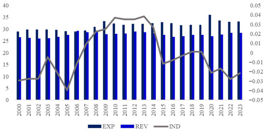
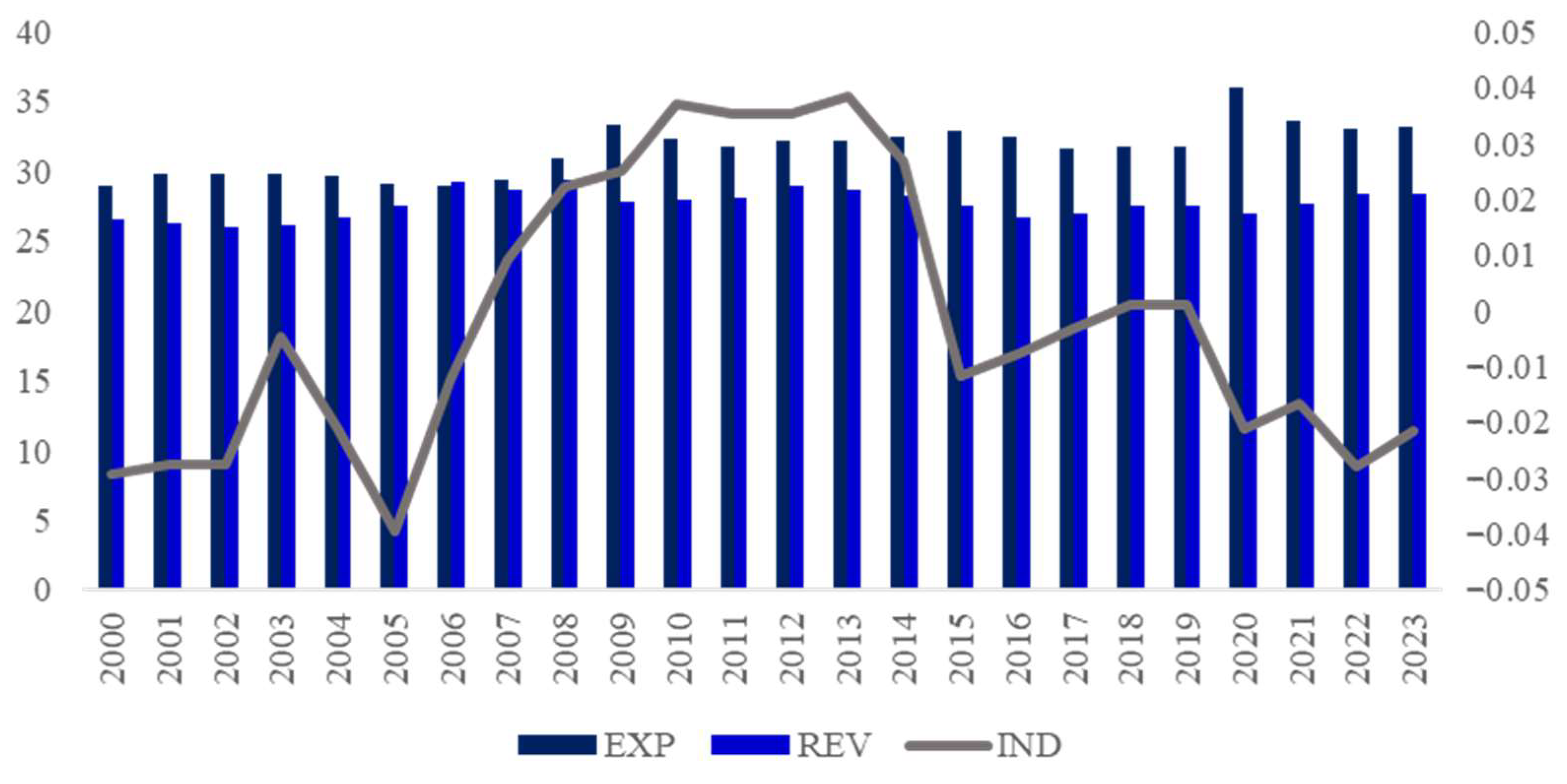
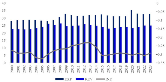
Over the period 2000 to 2023, Figure 1 shows an upward trend in public expenditure (EXP), rising from around 28.9% to over 33% of GDP on average, peaking in 2020 (36%) in response to the economic effects of the COVID-19 pandemic for the study sample. In contrast, public revenue (REV) has grown more moderately, averaging around 26–28% of GDP, suggesting a widening budget imbalance over time. At the same time, average institutional quality (IND) remains low overall, fluctuating around the neutrality threshold, with some improvements observed between 2007 and 2014, before experiencing a gradual decline. These developments reflect growing pressures on public finances in an unstable global context, marked by exogenous shocks (COVID-19, the Russian–Ukrainian war, Sino-tensions, conflicts in the Middle East) that have increased pressure on governments, particularly those with more fragile governance.
Figure 1.
Changes in revenue, expenditure and the overall institutional quality index. Source: authors, based on IMF and World Bank data.
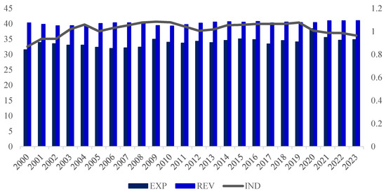
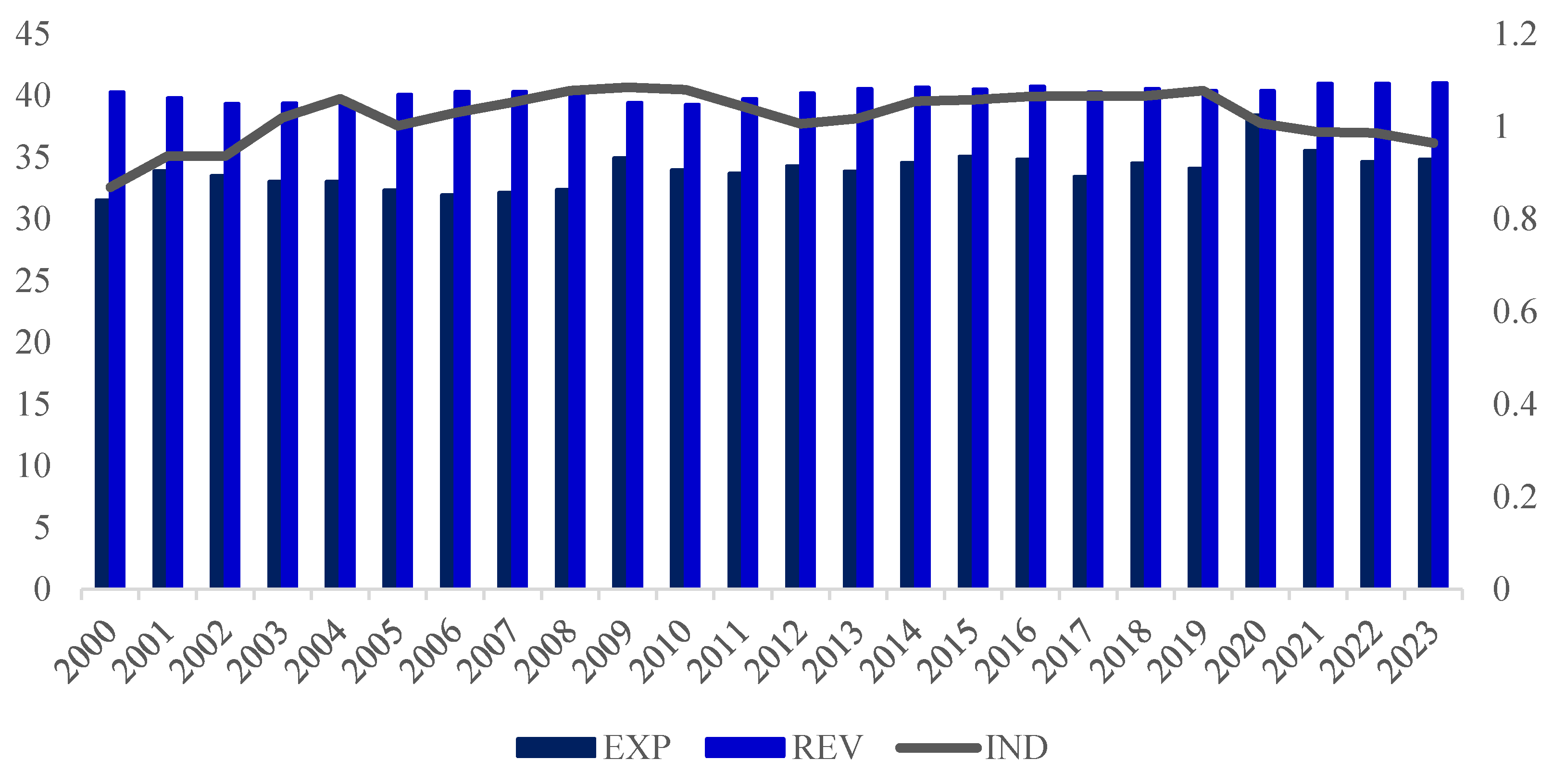
Analysis of Figure 2 below reveals that developed countries generally posted a structural primary surplus. Between 2000 and 2023, they followed a fiscal trajectory characterized by a sustained level of public revenue, exceeding 40% of GDP, reflecting a solid tax collection capacity supported by efficient institutions. Public expenditure, meanwhile, fluctuated between 32% and 35%, with two notable peaks in 2009 and 2020, corresponding respectively to the global financial crisis and the COVID-19 pandemic. This temporary increase in expenditure illustrates the fiscal responsiveness to systemic shocks. At the same time, institutional quality, which had initially been improving, began to erode from 2020 onwards, under the combined effect of internal political tensions, the contested management of successive crises, and increased geopolitical uncertainties, such as the Russian–Ukrainian war and trade conflicts.
Figure 2.
Evolution of revenue, expenditure and the institutional quality index of developed countries. Source: authors, based on data from the IMF and the World Bank.
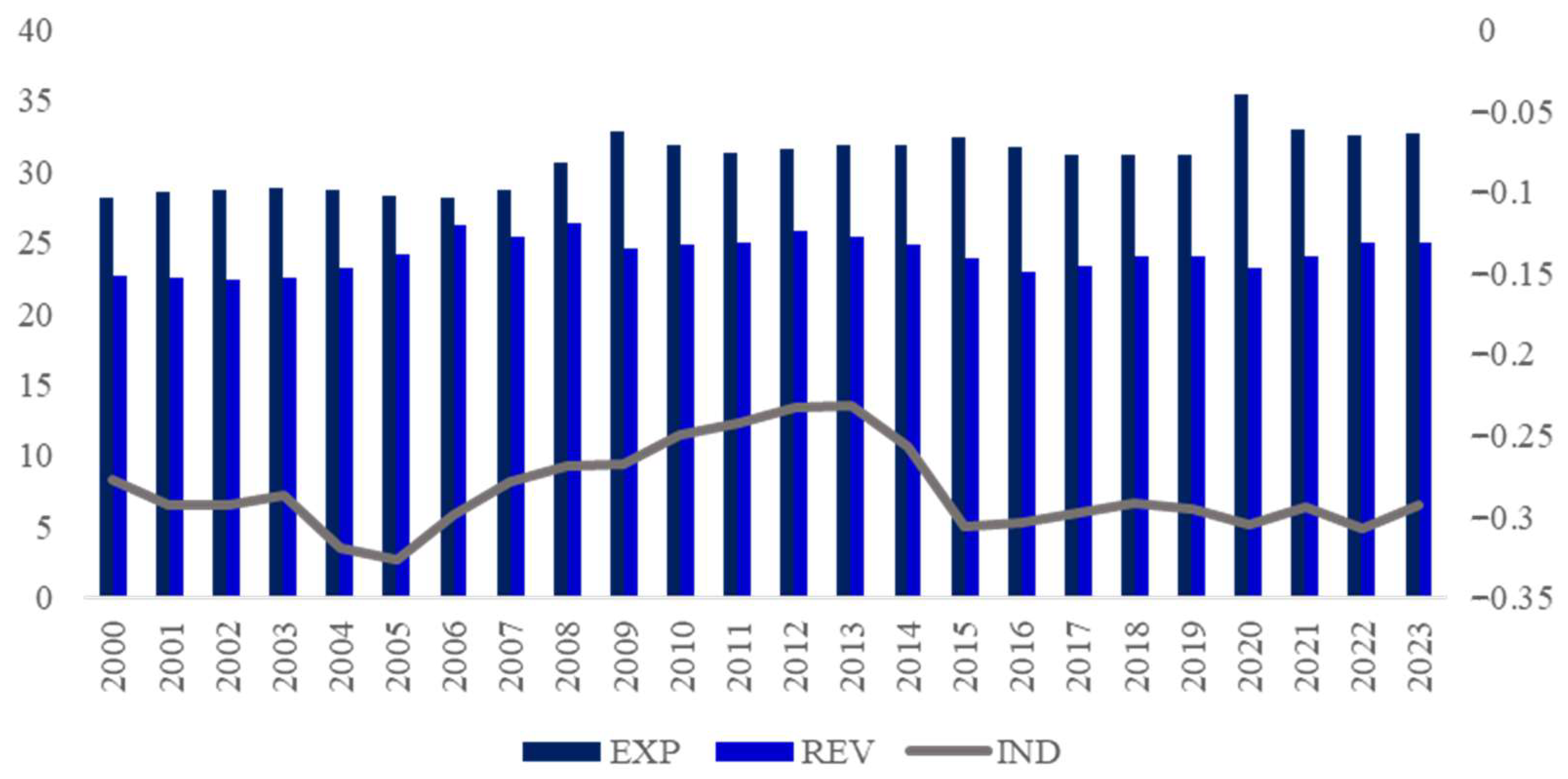
From 2000 to 2023, developing countries saw a gradual increase in average public spending, from 28.2% to nearly 32.7% of GDP, with a sharp peak in 2020 (35.4%) linked to the fiscal response to the COVID-19 pandemic (see Figure 3). In contrast, public revenues grew more moderately, fluctuating between 22% and 25% of GDP, reflecting a still limited fiscal capacity despite increased financing needs. This growing divergence between expenditure and revenue highlights a persistent structural deficit. At the same time, institutional quality (measured by the IND indicator) remained negative throughout the period, reflecting generally weak governance, despite a slight improvement between 2010 and 2014, followed by a further deterioration.
Figure 3.
Evolution of revenues, expenditures and the institutional quality index of emerging countries. Source: authors, based on IMF and World Bank data.
3. Review of the Literature
Barro’s (1979) contributions on Ricardian equivalence paved the way for a wealth of empirical literature analyzing the relationship between public revenue and expenditure. This literature provides contrasting results as to the direction of this relationship. In the short term, empirical verification of the relationship has developed around causality tests and VAR models. In the long term, however, the analysis is generally based on a linear cointegration relationship between public revenue and expenditure (Hakkio & Rush, 1991; Trehan & Walsh, 1991; Bohn, 1991; Quintos, 1995).
The meta-analysis by Gemmell et al. (2016) covering 28 OECD countries estimates revenue–expenditure elasticity at 0.38 in the short term and 0.52 in the long term, with particularly marked sensitivity during periods of recession. Furthermore, the work of Gupta (2019) on 45 emerging economies revealed more volatile elasticities and a significant impact of exchange rate shocks. Using a VECM model for the period 1981–2016, Uche and Ogbonna (2018) studied the relationship between public revenue and expenditure in Nigeria. The results reveal the existence of a unidirectional causality from expenditure to revenue, in line with the theory of Peacock and Wiseman (2024) and Musgrave and Musgrave (1989). Kazungu (2019) uses quarterly data for Tanzania to test the causality between public revenue and expenditure. He concludes that public expenditure is exogenous to Tanzanian public revenue.
However, Meher (2020) uses a VECM model to determine the short- and long-term relationship between public revenue and expenditure in Odisha over the period 1981–2017. The results show that there is a long-term unidirectional causality from revenue to public expenditure. However, the results do not confirm the existence of a short-term causal relationship between revenue and public expenditure. Similarly, Dritsaki (2018) uses an ARDL approach to annual data from Greece covering the period 1980–2015. His results confirm the theory of Buchanan and Wagner (1978), according to which revenue causes spending. Using the same approach, Adebisi and Salako (2020) find no evidence of long-term cointegration, but still show a causality from revenue to spending for Nigeria over the period 1961–2016. The same results are obtained by Saunoris (2015) for the United States over the period 1951–2008.
The fiscal synchronization theory has been confirmed by several empirical studies. Kaya and Arslan (2020) examine the asymmetric relationship between public revenues and expenditures in Turkey using quarterly data covering the period 2006–2019. They find a bidirectional asymmetric causality between the two fiscal variables. Oumer and Ramakrishna (2020) analyze the dynamics between public expenditure and revenue in Ethiopia over the period 1974–2016, using the NARDL approach. Their results show an asymmetric relationship, both in the short and long term, between actual revenue and actual expenditure. The asymmetric and bidirectional nature of causality implies that spending and revenue decisions are made simultaneously. From this perspective, Chang and Chiang (2009) analyze a sample of 15 OECD countries over the period 1992–2006 using a panel VECM model. The results reveal bidirectional causality for all countries in the sample. Ho and Huang (2009) also apply a panel VECM model to data covering the period 1999–2005 for 31 Chinese provinces. They find no significant short-term causal relationship between public revenue and expenditure. However, in the long term, their results confirm bidirectional causality, thus validating the fiscal synchronization hypothesis.
Finally, Brady and Magazzino (2018) test the causality between public revenue and expenditure in a panel of 28 European countries over the period 1980–2015. The results of the causality test by Dumitrescu and Hurlin (2012) indicate no causal link between the two variables for the sample as a whole, which corroborates the institutional separation hypothesis put forward by Baghestani and McNown (1994).
Recent empirical literature on the link between public spending and revenue generally focuses on verifying the existence of causality between these two budgetary variables. However, some studies address this relationship through the fiscal multiplier channel without providing conclusive results on the direct role played by institutional quality in this relationship. The first group of studies focuses on the link between public spending and economic growth, the role of institutional quality, income inequality, unemployment, and sustainable development (Turnovsky & Erauskin, 2022; Nguyen & Bui, 2022; Buthelezi, 2023; Tran Pham, 2025; Le et al., 2025; Ayana, 2026). A bidirectional relationship between public spending and economic growth has been highlighted by the findings of Nguyen and Bui (2022) and Buthelezi (2023). Using an international panel of 91 developing and 31 developed countries, Sidek (2021) found a negative relationship between public spending and income inequality. Furthermore, he found that for developed countries, public spending had to exceed a certain threshold in order to have an effect on reducing income inequality. The work of Le et al. (2025) on a sample of 46 developing economies revealed that public spending contributes positively and significantly to development when accompanied by a coherent and robust institutional framework. Finally, in a panel of 113 developed and developing economies, the results of Khan et al. (2024) proved that the relationship between public spending and economic growth improves in the long term when institutional quality is strengthened.
The second group provides empirical evidence on the effects of public revenue and expenditure on economic growth (Roşoiu, 2015), incorporating institutional quality (Ayana et al., 2024). Gurdal et al. (2021) examine the causal relationship between tax revenues, public spending, and economic growth in G7 countries over the period 1980–2016. The results show that there is a bidirectional short- and long-term causality between economic growth and tax revenues, and a long-term causality between economic growth and public spending. The results of Ayana et al. (2024) show that, based on a panel of 43 sub-Saharan African countries, public revenues have a negative impact on economic growth, while institutional quality has a positive and significant impact on economic growth. Finally, the significant results illustrated by the work of Mauro (2017), Acemoglu and Restrepo (2020), and Cabral (2017) show that improved control of corruption, regulatory quality, and political stability strengthen the capacity to mobilize domestic resources.
4. Methodological Approach
In panel data analysis, checking for inter-individual dependence is an essential statistical approach. Several methods have been developed for this purpose, some of which are preferred depending on whether the panel is balanced or unbalanced, as well as its size (small or large). Among the most commonly used are the LM test by Breusch and Pagan (1980); Pesaran’s (2004) adjusted LM; Pesaran’s (2015, 2021) CD tests; Juodis and Reese’s (2022) CDw; Fan et al.’s (2015) CDw+; and Pesaran and Xie’s (2021) CD*. These tests can be applied directly to the variables or to the estimated residuals of an individual fixed effects model.
4.1. Tests for Inter-Individual Dependencies
In this study, we use the last four tests, which we apply to the residuals from the fixed-effects model. The equations below show the statistics associated with each of these tests:
- Pesaran (2015, 2021):Juodis and Reese (2022):Fan et al. (2015):Pesaran and Xie (2021):with , and .
All of these tests are based on the same assumptions: the null hypothesis posits weak cross-dependence between units (independence or negligible dependence), while the alternative hypothesis assumes strong cross-dependence (significant correlation between residuals).
4.2. Panel Heterogeneity Tests
The literature on heterogeneity tests groups them into two main categories. Their importance lies in strengthening the robustness of estimates by ensuring that the model takes into account both cross-sectional dependence and heterogeneity within the panel. The first category, illustrated by the Pesaran and Yamagata (2008) test, helps guide the choice between fixed-effects and random-effects models by emphasizing the correlation between individual characteristics and independent variables. In contrast, the second category, proposed by Blomquist and Westerlund (2013), has the particularity of simultaneously taking into account cross-sectional dependence and individual-specificity. Pesaran and Yamagata (2008) propose the following two statistics for this purpose:
The literature on heterogeneity tests classifies these tests into two categories. The importance of these tests is to ensure the robustness of the estimates by ensuring that the model takes into account both cross-sectional dependence and panel heterogeneity. The first category, which includes the Pesaran and Yamagata (2008) test, helps to choose between the appropriate fixed-effects and random-effects model by emphasizing the correlation between individual characteristics and independent variables. In contrast, the second category, proposed by Blomquist and Westerlund (2013), has the particularity of simultaneously taking into account cross-sectional dependence and individual-specific heterogeneity. Pesaran and Yamagata (2008) propose the following two statistics:
Blomquist and Westerlund (2013), for their part, developed statistics given by:
For both tests, the null and alternative hypotheses relating to parameter homogeneity are formulated as follows:
Homogeneity of parameters
Heterogeneity of parameters
4.3. Panel Causality Test in the Presence of Heterogeneity
To examine the existence of a causal relationship between two variables in a heterogeneous panel, Dumitrescu and Hurlin (2012) developed a statistical technique that we use in this study. The presence of heterogeneity implies that the causal link within the sample may vary across individual units, as illustrated by the following equations:
The equations below describe the causal relationship between the variables and at different periods and for different cross-sectional units. The coefficients ; and represent the parameters associated with the lagged explanatory variables. The error terms are denoted and , respectively. In summary, the test hypotheses are as follows:
Based on these assumptions, Dumitrescu and Hurlin (2012) propose a mean statistic associated with the null hypothesis of homogeneous non-causality.
4.4. Pesaran’s (2007) CADF Stationarity Test
To account for cross-sectional dependence in panel data, Pesaran (2007) proposes the Cross-sectionally Augmented Dickey–Fuller (CADF) unit root test, which enhances the classic ADF test by adding cross-sectional means of levels and first differences of variables in order to control for unobserved common influences. In this study, we use Pesaran’s (2007) stationarity test, as it is suitable for large panels with high cross-dependence. Unlike first-generation tests, this test avoids biases due to the omission of common factors. Furthermore, the work of Hurlin and Mignon (2005) provided a summary of the main panel stationarity tests, including the CADF test by Pesaran (2007) used in this study. The form of the CADF regression can be specified as follows:
is the cross-sectional mean of ; is the cross-sectional mean of the first differences of ; the unit-specific coefficients are given by , , , ; and is the random term.
The null hypothesis of non-homogeneous stationarity is formulated as follows:
for all against the potentially heterogeneous alternative:
4.5. Cointegration Test in a Heterogeneous Panel
Identifying a long-term equilibrium relationship between non-stationary variables in a heterogeneous panel is a necessary preliminary step for applying econometric models that incorporate short- and long-term dynamics. To this end, several panel data cointegration tests have been developed in the econometric literature. Among the most robust and commonly used are the tests developed by Pedroni (1999), Kao (1999), and Westerlund (2007). In this study, we use the panel cointegration test proposed by Pedroni (1999) to examine the equilibrium relationship between variables because of its reliability and accuracy. This test allows us to verify the existence of a long-term cointegration relationship before estimating the associated parameters. It is particularly applicable in the presence of cross-sectional dependence, heterogeneity, and a unit root (Hurlin & Mignon, 2005). The basic equation used in the Pedroni (1999) test can be specified as follows:
is the dependent variable; is the individual fixed effect; is an individual linear trend; are the parameters associated with the matrix of independent variables ; is the error term and is tested for stationarity. Based on this equation, the author proposes seven statistics (parametric, semi-parametric and non-parametric), including four within-group (within-dimension) and three between-group (between-dimension) statistics based on the estimated residuals . In this framework, the regression of the residuals is written as follows:
The within-group statistics are based on an alternative hypothesis of homogeneous cointegration and are given by:
Panel v-Statistic:
Panel rho-Statistic:
Panel PP-Statistic (adjusted Phillips–Perron):
Panel ADF-Statistic (augmented Dickey–Fuller):
Inter-group statistics (between-dimension) are based on the alternative hypothesis of heterogeneous cointegration for at least one group of individuals and are given by:
Group rho-statistic:
Group PP-Statistic (adjusted Phillips–Perron):
Group ADF-Statistic (Augmented Dickey–Fuller):
4.6. CS ARDL Panel Model
In this research, we use a second-generation panel model known as the Cross-Sectionally Augmented Time Series Autoregressive Model (CS ARDL) developed by Chudik and Pesaran (2015). This model has several advantages over alternative econometric methods. First, it allows for the simultaneous estimation of short- and long-term relationships. Second, it offers the crucial advantage of being able to integrate variables with different integration orders. Third, it incorporates a lagged dependent variable and a lagged cross-sectional mean. This model is a generalization of the classic ARDL panel, within the framework of the dynamic common correlation estimator, taking into account both sample heterogeneity and unobserved common factors (Chudik et al., 2017). In this study, the CS-ARDL model captures the temporal and structural heterogeneity of the countries studied, taking into account cross-dependencies and national specificities, providing robust results for the formulation of differentiated fiscal policies adapted to the institutional context. The general form of the CS ARDL model can be expressed as follows:
where is the dependent variable; is a matrix of independent variables; is the cross-sectional mean defined by ; ; ; and denote the number of lags for each type of variable; is the error term.
Based on the previous general equation, the long-term parameters can be obtained using the Grouped Means (GM) method, and are as follows:
The error correction form of the CS ARDL model is then written as follows:
is the dependent variable; is the matrix of independent variables; and represent cross-sectional effects, capturing interdependencies between units; the parameters of the delayed cross-sectional means; and are the short-term dynamic components; and are the short-term coefficients; and are the short-term cross-sectional effects; measures the speed of adjustment towards long-term equilibrium; the long-term coefficients; and capture the sensitivity to average shocks in the system; is the error term.
5. Results and Discussion
The governance index (IND) was constructed using Principal Component Analysis (PCA) based on five indicators from the World Bank database (Kaufmann et al., 2010). These are Government Effectiveness (GE), Voice and Accountability (VA), Control of Corruption (CC), Political Stability (PSAT), and Regulatory Quality (RQ). The composite index thus obtained is then used in conjunction with public expenditure to capture the moderating effect on the budgetary impact.
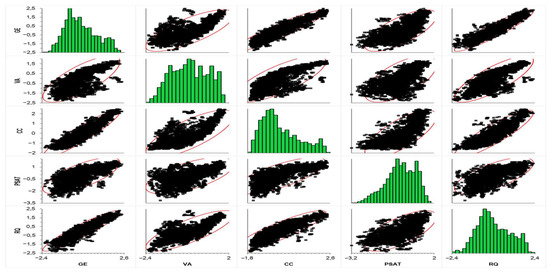
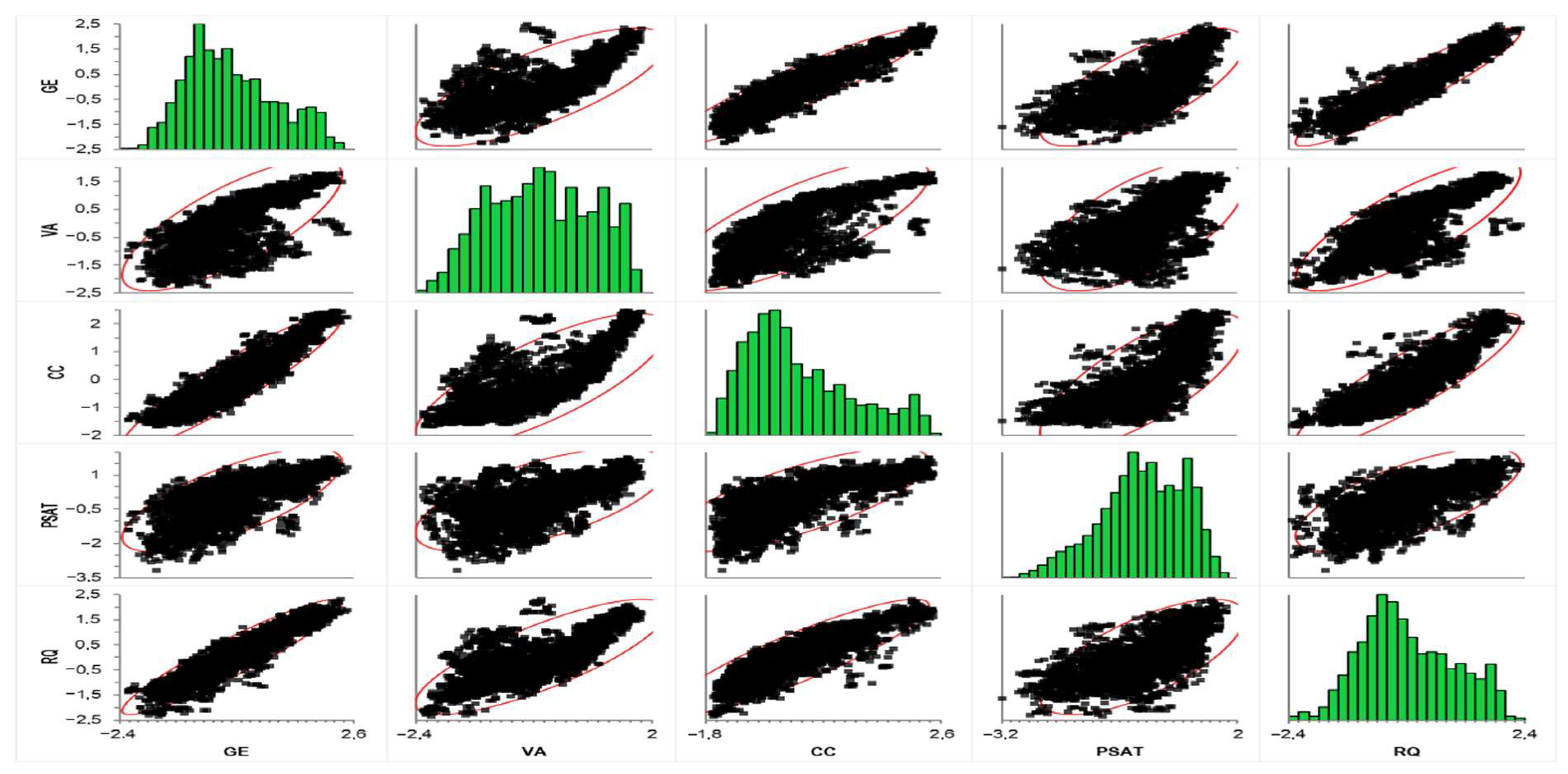
The procedure for constructing the institutional quality index is as follows: the study begins with an analysis of the correlation matrix and the multivariate correlations (Table 1 and Figure 4), which show that the five governance indicators are all positively and significantly correlated with each other, which fully justifies their aggregation into a composite index via PCA. Pearson’s correlation coefficients, which are consistently above 0.70, reveal very strong linear relationships, indicating that these dimensions of governance evolve in concert. The confirmation of these robust links by Spearman’s (rho) and Kendall’s (tau B) nonparametric rank tests attests that these associations are not sensitive to the precise form of the relationship or to any extreme values. This strong common covariance suggests the existence of a single, dominant latent dimension of “Governance” that PCA can effectively capture.
Table 1.
Multivariate correlation.
Figure 4.
Multivariate dynamic correlation. Source: authors, based on World Bank data.
The results in Table 2 of Bartlett’s sphericity test and the KMO (Kaiser–Meyer–Olkin) test confirm very robustly that the data are suitable for Principal Component Analysis (PCA). Bartlett’s test rejects the hypothesis that the variables are uncorrelated, indicating the existence of a strong latent structure between the governance indicators. In addition, the overall KMO measure of 0.866 is well above 0.80, meaning that the data share significant common variance, which is ideal for factor extraction. Finally, the individual MSAs, all above 0.79, show that each indicator is very well predicted by the others, confirming their internal consistency and their belonging to the same construct (index). In short, these tests guarantee the relevance and reliability of the PCA method.
Table 2.
Results of the KMO and Bartlett tests.
The Table of eigenvalues reveals a three-dimensional factor structure for the governance index, rather than the one-dimensional structure that might have been expected (Table 3). According to Kaiser’s criterion (eigenvalue > 1), three components should be retained: the first (eigenvalue = 2.12) explains 42.4% of the total variance, the second (1.28) 25.7%, and the third (1.27) 25.4%. Together, these three components capture a very high proportion of the information (93.5% of the total variance), which is excellent. This structure of three distinct factors, rather than a single one, suggests that the five governance indicators are grouped according to different underlying conceptual dimensions. The index (IND) is thus constructed based on the scores of the three dimensions and by taking into account the weight of each of them.
Table 3.
PCA results (solution with varimax rotation).
The three reliability coefficients—Cronbach’s alpha (α = 0.949), the standardized alpha coefficient (α = 0.949), and McDonald’s omega (ω = 0.947)—are high and virtually identical, providing very strong statistical evidence of the perfect internal consistency of the composite governance index. These results indicate that it captures the same single latent concept in a highly reliable and consistent manner. The extreme proximity of the alpha and omega values also suggests that the tau-equivalence hypothesis (equal weights for all items) is not problematic here, thus validating the simple weighted average construction method. In short, regardless of the coefficient considered, the IND index has a reliability well above the conventional thresholds of excellence (0.90), guaranteeing its robustness and stability.
In this subsection, we present the preliminary results of the analysis. First, Table 4 presents the description of the variables used in this study as well as the data sources for the 162 countries over the period 2000 to 2023. The data come mainly from the International Monetary Fund (IMF) and the World Bank (WB).
Table 4.
Variable description and data sources.
To classify the countries in the sample, the study adopts a binary methodological approach based on the 2022 HDI (UNDP Human Development Report 2023–2024), using a threshold of 0.800 to separate countries with very high human development from the others. Thus, developed countries are distinguished by an HDI ≥ 0.800 and developing countries by an HDI < 0.800.
The results of the descriptive statistics (Table 5) reveal that public revenues represent on average 27.69% of GDP with a high dispersion (12.55) and a minimum of 0.64% to a maximum of 85.78%. Public expenditure is higher on average, reaching 31.57% of GDP, with a minimum of 2.49%, a maximum of 133.28% and a standard deviation of 15.59. The governance index has a slightly negative average value close to zero (−0.002), reflecting a generally weak governance situation in all countries, but also significant institutional heterogeneity between countries, with extremes ranging from −2.17 to 2.83.
Table 5.
Summary statistics.
A comparative analysis of budgetary variables highlights significant disparities between developed and emerging countries. Developed countries have significantly higher average public revenues (REV) (40.18% ± 8.83) than emerging countries (24.24% ± 11.16), with a much smaller range (14.44–63.05% vs. 0.64–85.78%). In terms of expenditure (EXP), the average levels appear to be relatively closer between the two groups (33.92% ± 18.15 for developed countries and 30.92% ± 14.74 for emerging countries), but the latter are distinguished by more pronounced extreme values (2.49–133.28%), reflecting greater fiscal instability.
The governance index (GOV) is the most significant difference between the two categories of countries. Developed economies have a clearly positive average score (1.02 ± 0.49), while emerging countries have a negative average (−0.28 ± 0.68). This institutional divergence, combined with the increased volatility of fiscal indicators in emerging economies, suggests a close link between the quality of governance, the effectiveness of public policies, and the stability of public finances.
Similarly, analysis of the REVIND and EXPIND interaction variables highlights starkly contrasting budgetary dynamics between developed and emerging countries. Developed countries have clearly positive REVIND values (40.19 ± 19.71), reflecting the fact that their higher institutional quality is accompanied by an increased capacity to mobilize revenue. Conversely, emerging countries have a negative REVIND average (−5.43 ± 18.67), revealing that institutional weakness limits the generation of public revenues, with some extremely worrying situations (minimum of −129.88).
The divergence is even more pronounced in terms of the EXPIND variable. In developed countries, the interaction between governance and public spending remains positive (32.66 ± 20.21), a sign of more efficient budget management, where strong institutions reinforce spending efficiency. In contrast, emerging countries have a strongly negative EXPIND average (−9.69 ± 24.93), with very low minimums (−200.30). These extreme values reflect contexts where poor institutional quality leads to compression or efficiency in public spending, potentially to the detriment of essential services and productive investment. They thus support the hypothesis of an institutional crowding-out effect mentioned in the problem statement.
5.1. Results of Inter-Individual Dependence and Heterogeneity Tests
Table 6 presents the results of the inter-individual dependence and heterogeneity tests carried out in this study using four separate tests: the CD test by Pesaran (2015, 2021), the CDw test by Juodis and Reese (2022), the CDw+ test by Fan et al. (2015), and the CD* test by Pesaran and Xie (2021).
Table 6.
Cross-sectional dependence and slope heterogeneity.
The results reveal a strong and significant cross-sectional dependence in the entire sample as well as in each of the subgroups, as indicated by the CD, CDw, and CDw+ statistics, all of which are significant. This dependence reflects the fact that economic shocks spread simultaneously across the countries in the sample, reflecting the intensity of economic, trade, and financial interconnections at the global level. The particularly high value observed for emerging countries (CDw+ = 13,433.29) reflects an increased sensitivity of these economies to international contagion phenomena, often due to their greater exposure to external fluctuations, shallower financial markets, and more pronounced macroeconomic vulnerability.
The heterogeneity of slopes also appears significant across all groups, as confirmed by the Pesaran and Yamagata (2008) and Blomquist and Westerlund (2013) tests. These results, which are essential for empirical estimation, indicate that the relationships between variables differ structurally from one country to another, leading to the rejection of the hypothesis of coefficient homogeneity. Heterogeneity is particularly marked for all countries (Delta-adj = 34.558) as well as for emerging countries (Delta-adj = 33.030), revealing the diversity of fiscal, institutional, and macroeconomic configurations. The comparison between groups shows that, even though developed countries exhibit less pronounced heterogeneity, it remains statistically significant (Delta-adj = 19.575). Furthermore, the lack of significance of the CD* test for the latter group suggests a different structure of cross-sectional dependence, which is probably more attenuated or more homogeneous. Overall, these results justify the use of econometric methods capable of simultaneously taking into account cross-sectional dependence and country heterogeneity, and confirm the relevance of a differentiated analysis between developed and emerging economies.
5.2. Results of Stationarity Tests in a Heterogeneous Panel
The second-generation stationarity test developed by Pesaran (2007) is used in this study. Table 7 presents the results of the Cross-sectionally Augmented Dickey–Fuller (CADF) stationarity test applied to all variables in the model. The CADF unit root tests reveal that most variables are integrated of order one I(1) in the three samples, becoming stationary in first differences. Only a few variables are exceptions: CROI is stationary at level I(0) for all groups, while CRED is I(0) only for developed and emerging countries. This predominance of I(1) variables justifies the use of econometric techniques adapted to non-stationary series, in particular the search for cointegration.
Table 7.
Stationarity test.
5.3. Results of Cointegration Tests in a Heterogeneous Panel
Table 8 presents the results of the Pedroni (1999) cointegration test applied to all countries in the sample, as well as to the two subgroups: developed countries and emerging countries. In particular, the Modified variance ratio, the Phillips–Perron t and the Augmented Dickey–Fuller t are all significant at the 1% level for both intra-group and inter-group statistics. These results indicate the existence of a robust cointegration relationship between the variables studied, both for the overall sample and for each of the two subgroups. This suggests that, despite the heterogeneous dynamics observed between developed and emerging countries, the variables in the model evolve jointly in the long term.
Table 8.
Pedroni (1999) cointegration test.
5.4. Results of the Dumitrescu and Hurlin (2012) Causality Test
Table 9 presents the results of the Dumitrescu and Hurlin (2012) causality test, applied to all countries in the sample. These results reveal a significant bidirectional causality between public expenditure (EXP) and public revenue (REV). The Z-bar and Z-bar tilde statistics, both significant at the 1% threshold, indicate that changes in expenditure influence revenue, and vice versa. This result suggests the existence of an interactive fiscal mechanism in which expenditure decisions can be adjusted according to available revenue, while tax collection efforts respond to expenditure requirements. This reciprocal link reflects active fiscal coordination, where the two levers of fiscal policy, namely revenue and expenditure, are dynamically coordinated to ensure fiscal sustainability.
Table 9.
Causality of Dumitrescu and Hurlin (2012).
Refining the analysis by country group, the bidirectional causality between public spending and public revenue is confirmed in both developed and emerging countries. In developed countries, this relationship could reflect strong institutional stability, enabling medium-term budget planning, where revenues and expenditures are mutually adjusted within the framework of fiscal rules or credible multi-year forecasts. In emerging economies, however, this dynamic can be explained more by the presence of structural budgetary constraints and frequent macroeconomic shocks, forcing the authorities to make reactive and iterative adjustments between spending policies and resource mobilization strategies. The strength of the link between the two fiscal variables, regardless of the economic context, thus highlights the importance of flexible, adaptive, and well-coordinated fiscal governance that is capable of responding effectively to uncertainties while maintaining a framework of sustainability.
5.5. Results of the CS ARDL Model
The estimates are based on the work of Islam et al. (2022) and Chudik et al. (2017), who argue that the CS-ARDL model considers a one-year lag of the regressed variable, making the regressors weakly exogenous in the error correction framework, which strengthens the robustness of the estimate. The results of the CS-ARDL model make it possible to analyze the dynamic and structural relationships between government revenues (REV) and their main fiscal and macroeconomic determinants for both the sample countries as a whole and the subgroups of developed and emerging countries (Table 10). This analysis is based on robust econometric estimates that simultaneously take into account the individual heterogeneity of countries and cross-sectional dependence, making the results empirically robust and economically consistent. The effects identified show specificities marked by their level of development, highlighting the importance of differentiating public resource mobilization strategies according to the institutional and economic contexts specific to each group of countries.
Table 10.
Results of CS ARDL (MG) model estimates.
In the short term, the results reveal a persistence of public revenues, illustrated by the positive and significant coefficient of the lagged variable L.REV in the three subsamples, including 0.148 for all countries, 0.329 for developed countries, and 0.120 for emerging countries. This phenomenon of fiscal inertia is more pronounced in developed economies, due to a more stable and institutionalized tax system, where revenues are less sensitive to economic shocks.
Current public expenditure (EXP) has a positive and significant effect on revenues in all the groups studied. The elasticity of revenues to expenditure increases with the level of development: 0.543 for all countries, 0.619 for developed countries, and 0.722 for emerging countries. This trend suggests that fiscal stimuli boost economic activity, and therefore tax revenues, with a greater multiplier effect in emerging countries, where public demand is a key driver of economic activity.
The effect of the interaction between public spending and institutional quality (EXPIND) is particularly significant. The estimated coefficients are high and statistically significant in all three specifications: 0.587 for the overall sample, 0.760 for developed countries, and 0.814 for emerging countries. These results highlight a strong complementarity between institutional efficiency and fiscal policy. In other words, at the same level of expenditure, the capacity to mobilize tax revenues is substantially enhanced when institutions are effective, the regulatory framework is reliable, and governance is efficient. The more pronounced effect in emerging countries indicates that gains in governance generate a proportionally higher fiscal impact there, due to greater room for improvement.
Credit to the private sector (CRED), used as an indicator of the level of financial development, has a positive and significant effect in the overall sample (0.367) and for developed countries (0.469), but remains insignificant in emerging countries. This heterogeneity reflects a financial system that is still poorly integrated into the tax system in developing economies and a banking sector that is more oriented towards consumer financing than productive investment, limiting its indirect effect on revenues.
Economic growth (CROI) clearly supports public revenues, as evidenced by the significant coefficients obtained for all groups: 0.623 for all countries, 0.161 for developed countries, and 0.361 for emerging countries. This reinforces the idea of a virtuous circle between growth and tax mobilization. In developed economies, growth is generally more stable, resulting in a weaker marginal effect, while in emerging economies, even moderate growth can lead to substantial tax gains. In contrast, imports (IMP) do not have a significant effect in the overall sample, but their impact is marked in developed countries (0.077) and very strong in emerging countries (0.706). This illustrates the dependence of emerging economies on customs duties and indirect taxes, which are often the main sources of revenue in a context of low direct taxation.
The error correction term (ECM) coefficients are negative and significant across all groups, with values of −0.852 for the overall sample, −0.671 for developed countries, and −0.880 for emerging countries. These results confirm the existence of a fiscal adjustment mechanism towards long-term equilibrium. The higher speed of adjustment in emerging countries reflects stricter fiscal constraints or stronger pressure from international lenders, requiring a rapid return to sustainable public finances.
The long-term relationships validate the short-term trends observed while highlighting the structural stability of the link between public spending, quality of governance, and tax revenue mobilization. The coefficients associated with public spending remain positive and significant across all groups: 0.487 for the overall sample; 0.594 for developed countries; and 0.412 for emerging countries. This confirms that current spending, when well targeted, improves tax collection in a sustainable manner.
The effect of the interaction between public spending and institutional quality (EXPIND) is sustained over the long term, with significant and particularly high effects in emerging countries (0.867) and developed countries (0.859), compared to 0.318 for the overall sample. This result suggests that institutions act not only as a facilitating framework in the short term, but also as catalysts for sustainable fiscal performance in the long term. In emerging countries, this can be interpreted as a requirement for institutional support for spending policies to ensure their effectiveness.
In the presence of effective institutions, even a substantial increase in public spending can remain compatible with fiscal sustainability. Indeed, when funds are allocated efficiently and control, audit, and accountability mechanisms function properly, the risks of waste, corruption, and resource loss are greatly reduced. In this case, public spending contributes more to growth and, ultimately, to broadening the tax base, thereby supporting the sustainability of public finances. Conversely, in a fragile institutional context, even moderate levels of spending can compromise sustainability. Institutional weaknesses encourage mismanagement, misappropriation, and administrative inefficiency, significantly reducing the potential economic impact of public spending. Moreover, the lack of transparency and accountability mechanisms hinders the necessary adjustments in the event of budgetary slippage, increasing the risks of medium- and long-term unsustainability.
Overall, the results confirm and extend the conclusions of recent empirical literature and the hypotheses formulated. They validate the central role of institutional quality as a catalyst for the effectiveness of fiscal policies (Khan et al., 2024; Le et al., 2025). However, the methodological approach and theoretical framework have made it possible to go further by addressing a frequently identified limitation: the difficulty of isolating the direct role of institutions in the expenditure–revenue channel. By explicitly modeling the interaction effect between expenditure and institutional quality, we show that the latter is not simply a control factor, but a multiplier of fiscal effectiveness. This mechanism explains why similar levels of expenditure can lead to different sustainability trajectories. Furthermore, by showing a positive and significant effect of expenditure (EXP) on revenue (REV), they do not deviate significantly from the line of work that identifies a fiscal multiplier (Gurdal et al., 2021). Finally, like the work of Sidek (2021), the results of this study highlight very different dynamics between developed and emerging countries, thus justifying the subgroup approach.
5.6. Robustness of Results
In order to verify the consistency and robustness of the results obtained using the CS-ARDL approach, the study used the PMG-ARDL method developed by Pesaran et al. (1999). The results obtained are presented in Table 11 below. These results show that the relationships between revenue (REV), expenditure (EXP), and cross-expenditure on the governance index (EXPIND) are positive and significant at the 1% threshold. Indeed, improved governance strengthens the impact of expenditure on revenue in both the short and long term in all countries in the sample, as well as in developed and emerging countries. Across the entire panel, the results reveal that a 1% increase in public expenditure leads to an increase in public revenue of approximately 0.015% in the long term and 0.143% in the short term. This impact is 0.111% in the long term and 0.165% in the short term when accompanied by an improvement in the level of governance.
Table 11.
Results of the Panel ARDL (PMG) model estimates.
For developed countries, the results show a positive and significant relationship in both the long term and the short term. They indicate a greater impact in the short term for cross-cutting governance expenditures (0.287). On the other hand, a 1% increase in public spending directly translates into a 0.18% increase in revenue in the short term and a 0.176% increase in the long term. This impact is greater in developed countries than in emerging countries (0.033). Finally, emerging countries stand out for their crucial need to improve their level of governance. The impact of public spending on revenues is greater in the short term (0.425) than in the long term (0.033). Combined with the governance index (EXPIND), the impact is 0.648 in the short term and 0.147 in the long term. Overall, the results estimated by the PMG-ARDL method confirm that all exogenous variables have a positive influence on public revenues in both developed and emerging countries. These influences are particularly significant for the variable (EXPIND) in both subsamples.
Finally, the study uses a random effects model to test the robustness of the long-term results (Table 12). These results are consistent with those obtained by the CS-ARDL and PMG-ARDL models in terms of sign and parameter significance. This excludes the influence of model configuration errors on the overall interpreted results. These estimates thus confirm the consistency and robustness with those obtained by the CS-ARDL panel approach.
Table 12.
Results of Random-effects GLS regression model estimates.
6. Conclusions and Economic Policy Implications
The empirical results show, consistently across the three country subgroups, that public spending has a positive and statistically significant effect on public revenues, both in the short and long term. This effect is significantly amplified by institutional quality, as revealed by the positive impact of the EXPIND interaction variable. This evidence of the moderating role of institutions is an important first contribution of the study: it highlights that the ability of spending to mobilize resources in a sustainable manner depends heavily on the effectiveness and credibility of institutional frameworks. Thus, fiscal reforms focused solely on the amounts spent, without improving the governance framework, are likely to have limited effects. Furthermore, the results of the causality test by Dumitrescu and Hurlin (2012) highlight a bidirectional causal link between public revenue and expenditure, both for the entire sample and for developed and emerging countries.
The second major contribution of this study lies in the use of a CS-ARDL specification on a large global sample. This approach captures complex budgetary dynamics that are often ignored by standard models, including asymmetric adjustments, group effects, and interdependencies between countries. The use of this advanced methodology makes the analysis more robust and strengthens the relevance of the results for a variety of political and economic contexts.
In addition, the study highlights a third original contribution, namely the existence of differentiated fiscal regimes according to the level of development. In emerging countries, public spending and its interaction with institutions have a stronger impact on public revenues, reflecting greater sensitivity to public action. In developed countries, tax systems appear more stable but remain influenced by institutional and financial channels. This typology offers useful analytical perspectives for the implementation of fiscal policies differentiated according to the stage of economic and financial development. The significance and negativity of the adjustment term in all estimates validate the existence of a stable long-term relationship between the variables. This fourth contribution reinforces the idea that fiscal policy is intertemporally sustainable, provided that it is part of a favorable institutional framework. Thus, strengthening public governance appears not only as a requirement for good management, but also as a structural lever for fiscal performance. In short, this study contributes to the literature by combining fiscal and institutional dimensions within a rigorous and comprehensive methodological framework. It invites policymakers to design fiscal policies that are more effective, sustainable, and adapted to institutional and economic contexts.
The significant effect of the EXPIND interaction variable shows that the quality of institutions determines the effectiveness of public spending on revenue mobilization. Countries should therefore invest in reforms relating to budget transparency, the fight against corruption, and the quality of spending. This would create an economic environment conducive to broadening the tax base without increasing tax rates. Similarly, the significance of the CRED variable implies that greater access to banking services, formalization of the informal sector, sound SME financing policies, and increased use of formal means of payment can better connect the financial and tax systems. In countries where foreign trade revenues remain significant (particularly emerging countries), it is strategic to improve customs management, reduce fraud, and diversify sources of tax revenue beyond customs duties. Finally, the negativity and significance of the adjustment term shows that fiscal imbalances are corrected over time. In this sense, countries could strengthen their fiscal governance through multi-year planning and thus the implementation of medium-term budgetary frameworks (MTBFs) and credible fiscal rules to ensure the sustainability of public finances and rigorous monitoring of fiscal balances, even during recovery phases, to guarantee macroeconomic stability.
However, the main limitation of this study is that the multiplier effect of institutional quality could be conditional on a minimum level of governance, which is not identified here. The model assumes a linear relationship between public spending, institutional quality, and revenue. However, it is plausible that this relationship is nonlinear. In particular, the catalytic effect of institutions could have threshold effects: an improvement in governance would only have a significant impact on the effectiveness of spending after exceeding a critical level of quality. Conversely, below a certain threshold, spending could have zero or negative fiscal returns, regardless of the amount. The results presented, although robust within the methodological framework adopted, must be interpreted taking into account this limitation, which opens up avenues for future research.
Author Contributions
Conceptualization, S.N.N., Z.-y.D.H. and B.S.; methodology, S.N.N., Z.-y.D.H. and B.S.; software, S.N.N. and Z.-y.D.H.; validation, S.N.N., Z.-y.D.H. and B.S.; formal analysis, S.N.N., Z.-y.D.H. and A.S.B.; data curation, S.N.N. and Z.-y.D.H.; writing—original draft preparation, S.N.N., Z.-y.D.H. and A.S.B., writing—review and editing, S.N.N. and A.S.B. All authors have read and agreed to the published version of the manuscript.
Funding
This research received no external funding.
Institutional Review Board Statement
Not applicable.
Informed Consent Statement
Not applicable.
Data Availability Statement
The original contributions presented in this study are included in the article. Further inquiries can be directed to the corresponding authors.
Acknowledgments
The authors would like to express their deep gratitude to Mouhamadou Lamine DIAL, Head of the Economics Department of the Faculty of Economics and Management (FASEG-UCAD), for the valuable time he devoted to carefully reading and correcting the first draft of this work, as well as for his insightful advice, which greatly improved the quality of this document.
Conflicts of Interest
The authors declare no conflicts of interest.
References
- Acemoglu, D., & Restrepo, P. (2020). Robots and jobs: Evidence from US labor markets. Journal of Political Economy, 128(6), 2188–2244. [Google Scholar] [CrossRef] [Scilit]
- Adebisi, D. G., & Salako, G. (2020). Fiscal policy sustainability in Nigeria: ARDL bounds testing technique. Asian Journal of Empirical Research, 10(3), 74–80. [Google Scholar] [CrossRef] [Scilit]
- Ayana, I. D. (2026). Evaluating Sub-Saharan Africa’s government expenditure, corruption control, and economic growth through the generalized method of moments technique. Discover Sustainability, 7(1), 81. [Google Scholar] [CrossRef] [Scilit]
- Ayana, I. D., Demissie, W. M., & Sore, A. G. (2024). On the government revenue on economic growth of Sub-Saharan Africa: Does institutional quality matter? Heliyon, 10(2), e24319. [Google Scholar] [CrossRef] [Scilit] [PubMed]
- Baghestani, H., & McNown, R. (1994). Do revenues or expenditures respond to budgetary imbalances? Southern Economic Journal, 61(2), 311–322. [Google Scholar] [CrossRef] [Scilit]
- Baharumshah, A. Z., Jibrilla, A. A., Sirag, A., Ali, H. S., & Muhammad, I. M. (2016). Public revenue-expenditure nexus in South Africa: Are there asymmetries? South African Journal of Economics, 84(4), 520–537. [Google Scholar] [CrossRef] [Scilit]
- Barro, R. J. (1979). On the determination of the public debt. Journal of Political Economy, 87(5), 940–971. [Google Scholar] [CrossRef] [Scilit]
- Blomquist, J., & Westerlund, J. (2013). Slope homogeneity test in large panels with serial correlation. Economics Letters, 121(3), 374–378. [Google Scholar] [CrossRef] [Scilit]
- Bohn, H. (1991). Budget balance through revenue or spending adjustments?: Some historical evidence for the United States. Journal of Monetary Economics, 27(3), 333–359. [Google Scholar] [CrossRef] [Scilit]
- Brady, G. L., & Magazzino, C. (2018). Fiscal sustainability in the EU. Atlantic Economic Journal, 46, 297–311. [Google Scholar] [CrossRef] [Scilit]
- Breusch, T. S., & Pagan, A. R. (1980). The lagrange multiplier test and its applications to model specification in econometrics. The Review of Economic Studies, 47(1), 239. [Google Scholar] [CrossRef] [Scilit]
- Buchanan, J. M., & Wagner, R. E. (1978). Dialogues on fiscal religion. Journal of Monetary Economics, 4(3), 627–636. [Google Scholar] [CrossRef] [Scilit]
- Buthelezi, E. M. (2023). Impact of government expenditure on economic growth in different states in South Africa. Cogent Economics & Finance, 11(1), 2209959. [Google Scholar] [CrossRef] [Scilit]
- Cabral, F. J. (2017). Risk of corruption for economic growth and poverty: The case of a developing country. Risk Governance & Control: Financial Markets & Institutions, 7(2), 129–139. [Google Scholar]
- Chang, T., & Chiang, G. (2009). Revisiting the government revenue-expenditure nexus: Evidence from 15 OECD countries based on the panel data approach. Czech Journal of Economics and Finance (Finance a uver), 59(2), 165–172. [Google Scholar]
- Chudik, A., Mohaddes, K., Pesaran, M. H., & Raissi, M. (2017). Does the debt threshold affect output growth? Journal of Economics and Statistics, 99(1), 135–150. [Google Scholar] [CrossRef] [Scilit]
- Chudik, A., & Pesaran, H. (2015). Large panel data models with cross-sectional dependence: A survey. In Oxford handbook of panel data (1st ed.). Oxford University Press. [Google Scholar]
- DFI. (2023). The worst global debt crisis in history: New data from debt service watch. Development Finance International. [Google Scholar]
- Dritsaki, C. (2018). Causality between spending and revenue in the case of Greece through Toda and Yamamoto methodology. Journal of Business and Economic Policy, 5(1), 9–21. [Google Scholar]
- Dumitrescu, E. I., & Hurlin, C. (2012). Testing for Granger non-causality in heterogeneous panels. Economic modeling, 29(4), 1450–1460. [Google Scholar] [CrossRef] [Scilit]
- Estevao, M., & Essl, S. (2022). When the debt crises hit, don’t simply blame the pandemic. Dostupné, 8(4), 2022. [Google Scholar]
- Fan, J., Liao, Y., & Yao, J. (2015). Power enhancement in high-dimensional cross-sectional tests. Econometrica, 83(4), 1497–1541. [Google Scholar] [CrossRef] [Scilit] [PubMed]
- Friedman, M. (1978). The limitations of tax limitation, policy review, summer, 7–14. International Library of Critical Writings in Economics, 153, 288–295. [Google Scholar]
- Gemmell, N., Kneller, R., & Sanz, I. (2016). Does the composition of public expenditure influence long-term GDP levels? Oxford Bulletin of Economics and Statistics, 78(4), 522–547. [Google Scholar] [CrossRef] [Scilit]
- Gupta, B. (2019). Falling behind and catching up: India’s transition from a colonial economy. The Economic History Review, 72(3), 803–827. [Google Scholar] [CrossRef] [Scilit]
- Gurdal, T., Aydin, M., & Inal, V. (2021). The relationship between tax revenue, government expenditure, and economic growth in G7 countries: New evidence from time and frequency domain approaches. Economic Change and Restructuring, 54(2), 305–337. [Google Scholar] [CrossRef] [Scilit]
- Hakkio, C. S., & Rush, M. (1991). Is the budget deficit “too large?”. Economic Inquiry, 29(3), 429–445. [Google Scholar] [CrossRef] [Scilit]
- Ho, Y. H., & Huang, C. J. (2009). Tax-spend, spend-tax, or fiscal synchronization: A panel analysis of the Chinese provincial real data. Journal of Economics and Management, 5(2), 257–272. [Google Scholar]
- Hurlin, C., & Mignon, V. (2005). An Overview of Panel Unit-Root Tests. Economie & Prévision, (3), 253–294. [Google Scholar] [CrossRef] [Scilit]
- Islam, M. M., Sohag, K., Hammoudeh, S., Mariev, O., & Samargandi, N. (2022). Minerals import demands and clean energy transitions: A disaggregated analysis. Energy Economics, 113, 106205. [Google Scholar] [CrossRef] [Scilit]
- Juodis, A., & Reese, S. (2022). The problem of spurious parameters in residual cross-sectional correlation tests. Journal of Business & Economic Statistics, 40(3), 1191–1203. [Google Scholar]
- Kao, C. (1999). Spurious regression and residual-based tests for cointegration in panel data. Journal of Econometrics, 90(1), 1–44. [Google Scholar] [CrossRef] [Scilit]
- Kaufmann, D., Kraay, A., & Mastruzzi, M. (2010). The worldwide governance indicators: Methodology and analytical Issues (World Bank Policy Research Working Paper no. 5430). World Bank.
- Kaya, H. F., & Arslan, Ş. N. (2020). The government revenue–expenditure nexus: Asymmetric causality test. Current Research in Social Sciences, 6(2), 170–178. [Google Scholar] [CrossRef] [Scilit]
- Kazungu, K. (2019). The nexus between government expenditure and revenue in Tanzania. Asian Journal of Economic Modelling, 7(4), 158–170. [Google Scholar] [CrossRef] [Scilit]
- Khan, M., Raza, S., & Vo, X. V. (2024). Government spending and economic growth relationship: Can a better institutional quality fix the outcomes? The Singapore Economic Review, 69(01), 227–249. [Google Scholar] [CrossRef] [Scilit]
- Le, H. P., Nguyen, T. H. P., & Bao, H. H. G. (2025). Government expenditure and sustainable development in emerging markets: The role of institutional quality. Journal of Open Innovation: Technology, Market, and Complexity, 11(2), 100558. [Google Scholar] [CrossRef] [Scilit]
- Mauro, P. (2017). The effects of corruption on growth and public expenditure. In Political corruption (pp. 339–352). Routledge. [Google Scholar]
- Meher, S. (2020, January 8–10). Dynamic causal relationship between government expenditure and revenue in odisha: A trivariate analysis. 56th Annual Conference of the Indian Econometric Society (TIES), Madurai, India. [Google Scholar]
- Meltzer, A. H., & Richard, S. F. (1981). A rational theory of the size of government. Journal of Political Economy, 89(5), 914–927. [Google Scholar] [CrossRef] [Scilit]
- Musgrave, R. A., & Musgrave, P. B. (1989). Public finance in theory and practice, international edition (5th ed.). McGraw-Hill College. [Google Scholar]
- Nguyen, M. L. T., & Bui, N. T. (2022). Government expenditure and economic growth: Does the role of corruption control matter? Heliyon, 8(10), e10822. [Google Scholar] [CrossRef] [Scilit]
- North, D. C. (1990). Institutions, institutional change and economic performance. Cambridge University. [Google Scholar]
- OECD. (2025). Global debt report 2025: Financing growth in a challenging debt market environment. OECD Publishing. [Google Scholar]
- Oumer, H., & Ramakrishna, G. (2020, July 18–20). Government revenue, expenditure and fiscal deficits in Ethiopia: An asymmetric co-integration approach. Seventeenth International Conference on the Ethiopian Economy, Addis Ababa, Ethiopia. [Google Scholar]
- Peacock, A. T., & Wiseman, J. (1979). Approaches to the analysis of government expenditure growth. Public Finance Quarterly, 7(1), 3–23. [Google Scholar] [CrossRef] [Scilit]
- Peacock, A. T., & Wiseman, J. (2024). The growth of public expenditure in the United Kingdom. Taylor & Francis. [Google Scholar]
- Pedroni, P. (1999). Critical values for cointegration tests in heterogeneous panels with multiple regressors. Oxford Bulletin of Economics and Statistics, 61(S1), 653–670. [Google Scholar] [CrossRef]
- Pesaran, M. H. (2004). General diagnostic tests for cross section dependence in panels. Cambridge working papers. University of Cambridge. [Google Scholar]
- Pesaran, M. H. (2007). A simple panel unit root test in the presence of cross-section dependence. Journal of Applied Econometrics, 22(2), 265–312. [Google Scholar] [CrossRef] [Scilit]
- Pesaran, M. H. (2015). Testing weak cross-sectional dependence in large panels. Econometric Reviews, 34(6–10), 1089–1117. [Google Scholar] [CrossRef] [Scilit]
- Pesaran, M. H. (2021). General diagnostic tests for cross-sectional dependence in panels. Empirical Economics, 60(1), 13–50. [Google Scholar] [CrossRef] [Scilit]
- Pesaran, M. H., Shin, Y., & Smith, R. P. (1999). Pooled mean group estimation of dynamic heterogeneous panels. Journal of the American statistical Association, 94(446), 621–634. [Google Scholar] [CrossRef]
- Pesaran, M. H., & Xie, Y. (2021). A bias-corrected CD test for error cross-sectional dependence in panel data models with latent factors. arXiv, arXiv:2109.00408. [Google Scholar] [CrossRef] [Scilit]
- Pesaran, M. H., & Yamagata, T. (2008). Testing slope homogeneity in large panels. Journal of Econometrics, 142(1), 50–93. [Google Scholar] [CrossRef] [Scilit]
- Quintos, C. E. (1995). Sustainability of the deficit process with structural shifts. Journal of Business & Economic Statistics, 13(4), 409–417. [Google Scholar]
- Roşoiu, I. (2015). The impact of government revenues and expenditures on economic growth. Procedia Economics and Finance, 32, 526–533. [Google Scholar] [CrossRef] [Scilit]
- Saez, E., & Zucman, G. (2020). The rise of income and wealth inequality in America: Evidence from distributional macroeconomic accounts. Journal of Economic Perspectives, 34(4), 3–26. [Google Scholar] [CrossRef] [Scilit]
- Saunoris, J. W. (2015). The dynamics of the revenue–expenditure nexus: Evidence from US State government finances. Public Finance Review, 43(1), 108–134. [Google Scholar] [CrossRef] [Scilit]
- Sidek, N. Z. M. (2021). Do government expenditure reduce income inequality: Evidence from developing and developed countries. Studies in Economics and Finance, 38(2), 447–503. [Google Scholar] [CrossRef] [Scilit]
- Tran Pham, T. K. (2025). Impact of government expenditure on unemployment in Asian countries: Does institutional quality matter? International Journal of Development Issues, 24(2), 170–184. [Google Scholar] [CrossRef] [Scilit]
- Trehan, B., & Walsh, C. E. (1991). Testing intertemporal budget constraints: Theory and applications to US federal budget and current account deficits. Journal of Money, Credit and Banking, 23(2), 206–223. [Google Scholar] [CrossRef] [Scilit]
- Turnovsky, S. J., & Erauskin, I. (2022). Productive government expenditure and its impact on income inequality: Evidence from international panel data. Review of World Economics, 158(1), 331–364. [Google Scholar] [CrossRef] [Scilit]
- Uche, E., & Ogbonna, B. M. (2018). Tax-and-spend, spend-and-tax, fiscal synchronization, or fiscal separation: Emerging evidence from Nigeria. Journal of Economics and Sustainable Development, 9(24), 68–77. [Google Scholar]
- Westerlund, J. (2007). Testing for error correction in panel data. Oxford Bulletin of Economics and Statistics, 69(6), 709–748. [Google Scholar] [CrossRef] [Scilit]

Disclaimer/Publisher’s Note: The statements, opinions and data contained in all publications are solely those of the individual author(s) and contributor(s) and not of MDPI and/or the editor(s). MDPI and/or the editor(s) disclaim responsibility for any injury to people or property resulting from any ideas, methods, instructions or products referred to in the content. |
© 2026 by the authors. Licensee MDPI, Basel, Switzerland. This article is an open access article distributed under the terms and conditions of the Creative Commons Attribution (CC BY) license.