


Abstract
Carbon-intensive firms often remain locked into fossil-dependent technologies and assets even as carbon markets and environmental institutions improve, which matters for lenders, investors, and the design of transition finance. Using 333 Chinese high-carbon listed firms from 2016 to 2023, we build a four-dimensional carbon lock-in index and combine a panel-estimated feedback system, the power-sector coverage of China’s national emissions trading scheme, policy scenarios, and fuzzy-set qualitative comparative analysis. Own-state persistence dominates the system, and only a few cross-dimensional paths are discernible under any estimator. Carbon-market coverage lowered power firms’ institutional lock-in through carbon disclosure, the largest decline among eight high-carbon sectors, but did not reduce technological or market lock-in, and the composite index shows no robust decline. Financially constrained and unconstrained firms eased institutional lock-in by similar amounts, whereas firms with concentrated technical personnel did not ease even institutionally. After the reform, the one configuration that clears consistency and PRI thresholds joins financing constraints, state ownership, and concentrated technical personnel. Combined price and capital-expenditure shocks move projected lock-in by less than 3 percent. Transition finance should therefore be tied to verifiable technological redeployment rather than to disclosure alone.
Keywords:
carbon lock-in; financing constraints; transition finance; emissions trading scheme; capital expenditure; system dynamics; fuzzy-set qualitative comparative analysis; China JEL Classification:
G31; G32; Q54; Q58; O33; C32
1. Introduction
An uncomfortable pattern lies at the center of corporate decarbonization: environmental institutions can improve while carbon-intensive technologies and assets remain largely unchanged. Existing infrastructure already commits economies to substantial future emissions (Tong et al., 2019), but the investment, innovation, and compliance decisions that reproduce those commitments are made inside firms. Whether an institutional advance becomes technological and asset reconfiguration is therefore a question of corporate investment and finance: retiring long-lived assets and redirecting specialized capability require capital, and the terms on which firms raise it shape whether reform becomes decarbonization.
Three studies speak to this question but leave a gap between them. Carbon lock-in theory attributes persistence to increasing returns, sunk assets, institutional accommodation, and fossil-dependent markets that reinforce one another through dense feedback (Seto et al., 2016; Unruh, 2000, 2002); its evidence, however, comes from sectors and socio-technical regimes, and it does not tell us how permeable the boundaries between these elements are inside a firm. Research on carbon pricing documents what covered firms do, from emission reductions under China’s regional pilots (Cao et al., 2021; Cui et al., 2021) and directed innovation under the European market (Calel & Dechezleprêtre, 2016) to greenwashing by distressed Chinese firms (Tan et al., 2024), but each study observes one margin of response rather than the joint architecture of lock-in. Corporate-finance research shows that financing frictions raise pollution and shape firms’ responses to climate regulation (Bartram et al., 2022; Xu & Kim, 2022), and that investors and lenders price environmental performance (Bolton & Kacperczyk, 2021; Krueger et al., 2020; L. Liu, 2026); yet the measures it relies on, such as emission levels, carbon intensity, or ESG scores, do not reveal which part of a firm’s lock-in additional capital would reach. What is missing is a firm-level account of how lock-in is structured across dimensions, which dimensions a policy shock moves, and how financing conditions decide whether the response reaches technology and assets.
We address this gap with two concepts. Selective permeability means that each lock-in dimension reproduces itself while change crosses dimensional boundaries through only a few directional channels. It implies that a reform can produce dimensional easing, a fall in one component of lock-in, without structural unlocking, a change that weakens persistence or reaches technology and assets. Constraint migration means that when an institutional barrier is relaxed, the conditions that sustain high lock-in change rather than disappear, and may move toward the finance needed to redeploy incumbent capability. We ask how firm-level carbon lock-in persists across dimensions, which dimensions a carbon price moves, and how financing constraints and technical capability condition that response.
We study 333 Chinese A-share firms in eight high-carbon industries from 2016 to 2023, and each method answers a part of the question that the others cannot. A formative Carbon Lock-in Measurement Index (CLMI) separates technological, asset, institutional, and market lock-in, so that a change can be located in a dimension; an additive version of the index makes the composite exactly decomposable. A panel-estimated feedback system measures persistence and cross-dimensional transmission, which a single-equation design cannot. The national emissions trading scheme (ETS), which initially covered only power generation, supplies an observed price shock against which the system’s predictions can be tested in a difference-in-differences design, and splitting that design by financing constraints and technical personnel shows whether either changes the response. Scenarios translate the estimated system into the reach of price and capital-renewal levers, and fuzzy-set qualitative comparative analysis (fsQCA) asks which combinations of finance, ownership, and technical capability accompany high lock-in before and after the reform, a conjunctural question that regression averages cannot answer.
The evidence describes a selectively permeable system. All four dimensions show positive own-state persistence, which roughly doubles after a correction for dynamic-panel bias, while only one to four of the twelve cross-dimensional paths are discernible under fixed-effects, jackknife, and GMM estimators. ETS coverage lowered power firms’ institutional lock-in by 0.063 (0.40 standard deviations), the largest decline among the eight high-carbon sectors, through a rise in carbon disclosure that began when allowances were allocated in 2020. It did not reduce technological or market lock-in; power firms’ technological lock-in had been rising relative to other firms before the reform and stayed at its 2020 level afterwards. The composite index fell by 0.16 standard deviations in the baseline estimate, but the decline loses significance in six of the eleven alternative specifications, so the carbon-market effect is dimensional rather than aggregate. Financially constrained and unconstrained power firms eased institutional lock-in by similar amounts, and under none of the three financing measures do their institutional or technological responses differ significantly; by contrast, firms with concentrated technical personnel did not ease even institutionally. Before the reform, no combination of financing, ownership, and technical personnel is sufficient for high lock-in; after it, financially constrained state-owned firms with concentrated technical personnel form the one configuration that clears both the consistency and the PRI thresholds. Combined price and capital-expenditure shocks move the projected index by less than 3 percent under every estimator.
The paper makes three contributions. First, it qualifies the dense-coupling premise of carbon lock-in theory at the firm level: persistent dimensions linked by sparse paths imply that a policy can ease one dimension without unlocking the technology–asset core, and the carbon-market evidence shows this directly. Second, it adds to research on finance and corporate environmental behavior (Bartram et al., 2022; Tan et al., 2024; Xu & Kim, 2022) by locating where financing conditions bind within the lock-in architecture: financing constraints on their own did not change how far firms’ response to a carbon price reached, in disclosure or in technology, but after the reform they join concentrated technical capability in the configuration that sustains high lock-in, so finance binds in conjunction with capability rather than by itself. Third, it shows how measurement, dynamics, a quasi-experiment, and configurations can be combined so that each supplies evidence the others cannot, and it documents the measurement choices on which such a combination rests. For lenders, investors, and regulators, the implication is that disclosure-based progress is a weak signal of unlocking and that transition finance should be tied to verifiable technological redeployment.
2. Institutional Background
2.1. Carbon Pricing in China
China introduced carbon pricing through seven regional pilot markets launched in 2013 and 2014, which covered emitters in a few provinces and cities and reduced covered firms’ emissions (Cao et al., 2021; Cui et al., 2021). In September 2020, the government pledged to peak carbon dioxide emissions before 2030 and to reach carbon neutrality before 2060 (Mallapaty, 2020). The national ETS followed. In early 2021 the Ministry of Ecology and Environment allocated free allowances for 2019–2020 emissions to more than two thousand power generators on the basis of output-based intensity benchmarks, and trading opened in July 2021. Covered entities must monitor, verify, and report their emissions every year, and from 2022 entities in the national market have also had to disclose carbon-emission information under the national rules on corporate environmental information disclosure. The scheme therefore reached covered firms first through allocation, monitoring, reporting, and disclosure obligations, and only later through the price of allowances. The other high-carbon sectors in our sample remained outside the national market throughout 2016–2023; steel, cement, and aluminum smelting were brought in only from the 2024 compliance year.
2.2. Financing Conditions of High-Carbon Firms
High-carbon firms finance capital renewal largely through bank credit and retained earnings. Green-credit guidelines, green-finance pilot zones, and, from late 2021, central-bank relending for carbon-reduction projects have channeled cheaper credit toward certified low-carbon investment, and lenders and bond investors increasingly price environmental performance; in the Chinese bond market, firms with better ESG performance pay a lower cost of debt (L. Liu, 2026). A firm’s financing position therefore matters in two ways. It determines whether the firm can fund the replacement of carbon-intensive assets and the redeployment of its technical staff, and it shapes the incentive to improve the visible environmental indicators, such as disclosure, that lenders and investors observe. Ownership adds a further layer, because state-owned firms face policy mandates and have easier access to bank credit than private firms.
3. Theory and Hypotheses
We organize the analysis around three research questions. How strongly does each dimension of firm-level carbon lock-in reproduce itself, and how much change crosses dimensional boundaries? Which dimensions does a carbon price move? And how do financing constraints and technical capability condition the response, including the organizational conditions that accompany high lock-in before and after the reform? Each question yields a hypothesis that one part of the empirical design tests.
3.1. Persistence and Cross-Dimensional Permeability
Corporate carbon lock-in is not simply high current emissions. Emissions are a flow; lock-in is the structure that makes the flow difficult to change. At the firm level, that structure comprises carbon-specialized knowledge and production routines, long-lived physical assets, institutionalized governance and compliance practices, and dependence on carbon-intensive product and energy markets (Erickson et al., 2015; Seto et al., 2016; Unruh, 2000). We represent it as a state vector of technological, asset, institutional, and market lock-in. Path-dependence theory and the natural-resource-based view (NRBV) predict that each element reproduces itself: knowledge and routines accumulated around an incumbent technology lower the cost of continuing along that path (Aghion et al., 2016; Hart, 1995), and firms keep operating carbon-intensive assets because premature retirement destroys quasi-rents (Klitkou et al., 2015; Pfeiffer et al., 2016).
Two views differ on what happens across dimensions. Regime-level accounts describe lock-in as a techno-institutional complex in which the elements reinforce one another through dense feedback (Geels, 2014; Seto et al., 2016; Unruh, 2002); carried to the firm, this view predicts strong, mostly positive cross-dimensional links. An organizational view predicts the opposite. Budget ownership, asset specificity, and divisional boundaries can insulate one dimension from another: a compliance unit can adapt to a carbon market without production engineers replacing equipment, and a cleaner product-market signal need not release the finance required for capital renewal. If boundaries insulate, cross-dimensional links are few and directional, and a change in one dimension need not reach the others.
Hypothesis 1 (H1).
Each dimension of firm-level carbon lock-in displays positive own-state persistence, and within-dimension persistence is stronger than cross-dimensional transmission.
3.2. Carbon Pricing and Dimensional Easing
The induced-innovation view holds that a carbon price raises the return to clean technology and redirects innovation toward it (Aghion et al., 2016); covered European firms raised their low-carbon patenting (Calel & Dechezleprêtre, 2016). On this view, coverage should lower technological lock-in. Three features of China’s national ETS point instead to the institutional dimension. Covered firms met the scheme first through allocation, verification, and disclosure obligations (Section 2), which act directly on governance and reporting. Output-based intensity benchmarks with free allocation weaken the marginal incentive to cut total emissions. And the long life of power assets delays any asset response beyond a few years. Evidence that emissions trading raised greenwashing among Chinese firms (Tan et al., 2024) and that the pilots cut coal use through dispatch rather than plant efficiency (Cao et al., 2021) points the same way.
Hypothesis 2 (H2).
Coverage by the national ETS lowers covered firms’ institutional lock-in more than their technological, asset, or market lock-in.
3.3. Financing Constraints, Technical Capability, and Constraint Migration
Financing constraints can shape the response to a carbon price in opposite directions. Redirecting technology and replacing assets are investments, so constrained firms may lack the funds to undertake them; financially constrained firms pollute more (Xu & Kim, 2022). Yet constraints can also strengthen the incentive to act: constrained firms subject to carbon regulation shift emissions to unregulated plants rather than abate (Bartram et al., 2022), distressed firms answer emissions trading with greenwashing (Tan et al., 2024), and lenders reward visible environmental performance with cheaper debt (L. Liu, 2026). The two views can be reconciled by the cost of each margin of response. Disclosure is cheap and mandated, so the institutional response should not depend on finance; technological redirection is costly and uncertain, so it should come from firms that can fund it.
Hypothesis 3a (H3a).
Among firms covered by a carbon price, the technological response is concentrated among financially unconstrained firms, whereas the institutional response does not depend on financing constraints.
The NRBV treats technical capability as a resource for pollution prevention and environmental reconfiguration (Hart, 1995; Hart & Dowell, 2011), but accumulated technical expertise is not direction-neutral. With finance and a mandate to redeploy it, a concentrated technical workforce can absorb low-carbon processes; without them, the same workforce optimizes incumbent equipment and extends the life of carbon-intensive assets (Aghion et al., 2016; Fouquet, 2016). Before a reform, when external pressure is weak, high lock-in need not depend on a firm’s financing position. Once the institutional environment tightens, the firms that remain highly locked in should be those that hold concentrated incumbent capability but cannot finance its redeployment. The binding condition then migrates from the external institutional environment to the firm’s combination of finance and capability, which is what we call constraint migration. Because the effect is conjunctural, no single condition should be necessary on its own.
Hypothesis 3b (H3b).
After the reform, the configurations sufficient for high carbon lock-in join concentrated technical personnel with financing constraints, whereas before the reform they do not.
The empirical sequence follows the hypotheses. The CLMI establishes whether the four dimensions move together; the panel feedback system tests H1; the carbon-market design tests H2 and, split by financing constraints and technical personnel, H3a; and the pre- and post-reform fsQCA tests H3b. The scenarios translate the estimated system into the reach of distinct policy levers.
4. Materials and Methods
4.1. Sample Selection and Data Sources
The sample is built in four steps, summarized in Table 1. We start from all A-share firms classified, under the 2012 industry guidelines of the China Securities Regulatory Commission (CSRC), in the eight high-carbon divisions in which China’s industrial emissions are concentrated: paper (C22), petroleum processing (C25), chemicals (C26), non-metallic mineral products (C30), ferrous metals (C31), non-ferrous metals (C32), electricity and heat (D44), and air transport (G56). We restrict attention to these industries because technological path dependence, sunk carbon-intensive capital, and energy-supply rigidity are most acute there; extending the index to lower-carbon sectors is left for future work. Of the 789 firms in these divisions in at least one year of 2016–2023, we keep the 457 that are listed and classified in them in every year. A balanced panel is required for two reasons: the feedback system is estimated from consecutive annual transitions of the same firms, and the fsQCA compares the same 333 cases before and after the reform; holding the panel fixed also keeps each firm’s industry, and hence its ETS coverage, constant. We then drop 54 firms designated ST or *ST, or suspended, in any year, because financial distress distorts their reporting and investment. Finally, we drop 70 firms for which firm-level emissions or another of the nine CLMI sub-indicators could not be assembled for every year. The final sample contains 333 firms and 2664 firm-year observations.
Table 1.
Sample construction.
Corporate-level carbon dioxide emission data are obtained from firm environmental reports, corporate social responsibility (CSR) reports, and the China Emission Accounts and Datasets (CEADs). Financial and governance variables, including total assets, revenue, R&D expenditure, leverage, board characteristics, and ownership structure, are sourced from the China Stock Market and Accounting Research (CSMAR) database and the WIND Financial Terminal. Green patent data are retrieved from the China National Intellectual Property Administration (CNIPA) database, classified according to the International Patent Classification (IPC) green inventory. Provincial-level environmental regulation indicators are constructed through textual analysis of local government work reports, measuring the proportion of environment-related keywords. Energy consumption and energy intensity data at the provincial level are obtained from the China Energy Statistical Yearbook and the National Bureau of Statistics. ESG ratings, specifically the environmental sub-score (Escore), are sourced from the Huazheng ESG rating system. The KZ index of financing constraints and the cost of debt are taken from commercial compilations of financial-statement data for Chinese listed firms. Section 4.3 lists the definition, calculation, and source of each sub-indicator. Each sub-indicator except the high-carbon energy share, which ranges only from 98.98 to 99.28 percent, is winsorized at the 1st and 99th percentiles of the pooled 2016–2023 distribution before normalization; the four exogenous inputs are winsorized in the same way. In the final panel the nine sub-indicators and the firm controls contain no missing values; gaps in the provincial exogenous inputs were filled before estimation, and the three fsQCA conditions had gaps in 10 (SA), 39 (TechProp), and 92 (EI) of the 2664 firm-years, which we fill with industry-year means. Because corporate emission reporting is partly voluntary, we triangulate emission figures across firms’ environmental and CSR disclosures and CEADs, re-examining materially divergent observations; the large listed firms in our sample also face China’s most stringent disclosure obligations. An index rebuilt without the emission level ranks firms much like the full index (Spearman correlation 0.94; Table A4), so the dimensional results do not hinge on that single input. Residual disclosure-selection bias cannot be fully eliminated (Section 6.4).
4.2. Variable Construction and Descriptive Statistics
The core dependent variable is the Carbon Lock-in Measurement Index (CLMI), a composite index constructed from nine sub-indicators spanning four dimensions: Technological Lock-in (B1), Asset Lock-in (B2), Institutional Lock-in (B3), and Market Lock-in (B4). The technological dimension comprises emission levels, green patent ratio (GreenPat), and R&D intensity (RdInt). The asset dimension includes the logarithm of non-low-carbon fixed assets (NLFA) and the capital depreciation intensity (CapDeprInt). The institutional dimension captures environmental regulatory stringency (EnvReg) and institutional completeness (InstCompl). The market dimension is measured by carbon intensity (CarbonInt) and high-carbon energy dependence (HCEDD). Indicators are directionally unified so that higher values consistently correspond to deeper lock-in.
For the system dynamics analysis, four exogenous variables are introduced: national coal price (CoalPrice), capital expenditure ratio (CapEx), provincial industrial pollution control investment (PollInv), and provincial energy intensity (EnergyInt). Coal price is chosen as the energy-cost driver because coal is the dominant, price-setting marginal energy input across China’s high-carbon industries; PollInv and EnergyInt are included at the provincial level to capture the broader regulatory effort and energy-efficiency context. The fsQCA employs six condition variables: financing constraints (the KZ index), ownership type (OWN), technical personnel ratio (TechProp), market concentration (HHI), environmental protection intensity (EnvEff), and regional energy intensity (EI), alongside the CLMI as the outcome. Six firm-level controls are included in the regressions: firm size (SIZE), leverage (LEV), return on assets (ROA), ownership concentration (INDEP), board size (BSIZE), and board independence (OC). Full definitions and sources are reported in Table 2.
Table 2.
Definitions and data sources of firm-level variables used in the empirical analysis.
We measure financing constraints with the KZ index of Kaplan and Zingales (1997), estimated for Chinese listed firms by Wei et al. (2014) from operating cash flow, Tobin’s Q, leverage, dividends, and cash holdings, with higher values indicating tighter constraints. We do not use the size–age (SA) index of Hadlock and Pierce (2010) as the main measure, for two reasons that Table 3 documents. First, with total assets measured in RMB million, the index is negative for every firm-year in our sample (mean , range to ), so higher, less negative values indicate tighter constraints and its absolute value would rank firms in reverse. Second, the sample mean of log assets (9.03) lies close to the turning point of the index’s quadratic size term (8.57), so the size component varies little (from to between the 5th and 95th percentiles) and the cross-sectional variation of the index is dominated by firm age: its correlation with age is and with SIZE 0.22. The KZ index, by contrast, is correlated 0.57 with leverage and with return on assets, and only 0.09 with firm age. We use the SA index, in its original sign, and the cost of debt (interest expense over average interest-bearing debt) as alternative measures.
Table 3.
Descriptive statistics of the lock-in indices and firm-level conditions.
The composite CLMI has a mean of 0.341 and a standard deviation of 0.131, with values ranging from 0.000 to 0.998, and the additive index (Section 4.3) has a mean of 0.451 and a standard deviation of 0.072. Among the four dimensions, Institutional Lock-in exhibits the highest mean (0.658), while Market Lock-in records the lowest (0.182), indicating substantial cross-dimensional heterogeneity in lock-in severity. Table 3 reports the full distribution of the dimensional sub-indices, the two composite indices, and the financing-constraint and organizational conditions.
4.3. Operationalizing Carbon Lock-In as a Multidimensional State
Measuring corporate carbon lock-in requires a framework that captures its multidimensional, structurally embedded nature rather than single-proxy indicators such as total emissions or carbon intensity. We construct a Carbon Lock-in Measurement Index from nine sub-indicators across four theoretically grounded dimensions: technological, asset, institutional, and market lock-in (Table 4 summarizes the framework and the sign with which each sub-indicator enters the index). The contribution of this measurement architecture is not simply a new composite score. It retains the dimensional state vector needed to distinguish a lower observed level of lock-in from a change in the structure that reproduces it. The composite CLMI summarizes overall severity, whereas – reveal whether institutional or market easing penetrates the technology–asset core.
Table 4.
Structural framework, calculation, and sources of the carbon lock-in measurement index.
Grounded in the techno-institutional complex framework and the multidimensional lock-in typology, each sub-indicator proxies a distinct structural source of carbon dependence. The sub-indicators are formative and potentially interdependent: together they constitute lock-in rather than reflect a single latent factor. This motivates a two-stage strategy. We first aggregate indicators within and across dimensions to describe the state of lock-in; we then preserve the four-dimensional scores in the system-dynamics and configurational analyses to estimate permeability rather than assuming independence in a single-equation specification. A firm can consequently receive the same composite score through different dimensional architectures, an analytically important distinction because those architectures imply different policy responses.
Technological lock-in reflects the extent to which a firm’s innovation trajectory and production processes remain anchored to carbon-intensive paradigms, as captured by three sub-indicators. emission level (log of annual emissions) measures the absolute scale of carbon entrenchment. The green patent ratio (GreenPat), green low-carbon patents over total patents, captures the directionality of innovative effort and enters with a negative sign, since greater orientation toward clean technologies implies lower lock-in. R&D intensity (RdInt), R&D investment over revenue, also enters negatively, since greater capacity for technological renewal weakens attachment to incumbent paradigms.
Asset lock-in captures the extent to which long-lived, carbon-intensive physical capital constrains future emission pathways through sunk costs and irreversibility, comprising two sub-indicators. The logarithm of non-low-carbon fixed assets (NLFA, log of such investment plus one) reflects the scale of capital committed to carbon-intensive production, with higher values increasing the structural rigidity of the emission trajectory. Capital depreciation intensity (CapDeprInt), depreciation over gross book value, measures the annual charge at which the carbon-intensive capital stock is written down. Its orientation is not self-evident. In our baseline a higher intensity indicates deeper lock-in: a large annual depreciation charge is a fixed cost of installed carbon-intensive capacity that a firm recovers only by continuing to operate it, the sunk-cost logic by which capital stocks commit future emissions (Pfeiffer et al., 2016; Tong et al., 2019). The stranded-asset literature suggests the opposite reading, in which faster write-down shortens the remaining life of the capital stock and with it the emissions it commits. Because the two readings cannot be separated with the data assembled for the index, which do not include accumulated depreciation or remaining useful lives, we report every result that involves the asset dimension under both orientations (Table A7 and Figure A1). The asset-dimension effect of the carbon market is sensitive to the choice; the institutional, technological, and market results and the feedback architecture are not.
Institutional lock-in measures the extent to which regulatory environments and governance arrangements reinforce carbon-intensive operational patterns through two sub-indicators. Environmental regulatory stringency (EnvReg), the proportion of environmental keywords in government reports, captures policy attention to environmental governance and enters negatively, since stronger regulation pressures firms away from carbon-intensive operations. Institutional completeness (InstCompl), the frequency of carbon-related words in annual and CSR reports, reflects how far corporate disclosure and governance internalize carbon transition considerations and also enters negatively, since proactive engagement with decarbonization signals lower lock-in.
Market lock-in captures the structural dependencies in a firm’s product markets and energy consumption that perpetuate demand for carbon-intensive outputs, via two sub-indicators. Carbon intensity (CarbonInt), total emissions over revenue, measures the carbon embeddedness of revenue-generating activities, with higher values indicating a market position structurally dependent on carbon-intensive production. High-carbon energy dependence (HCEDD), the share of high-carbon energy in total energy consumption, captures reliance on fossil-fuel-based energy, with higher values indicating deeper entrenchment in carbon-intensive supply chains.
We normalize each sub-indicator to the unit interval by min–max normalization over the pooled 2016–2023 sample, reversing the scale of the four indicators that enter negatively. A common scale across firms and years keeps changes over time comparable, which the dynamic and quasi-experimental analyses require; persistent differences in the level of lock-in across industries are absorbed by firm fixed effects in those analyses, while the descriptive and configurational analyses compare firms across the high-carbon sectors as a whole (normalization within industry-year cells is left for future work; Section 6.4). To avoid subjective weighting bias, indicator weights follow an objective combined CRITIC–entropy scheme: the entropy component rewards indicators with greater information content, while the CRITIC component incorporates each indicator’s variability and its conflict (correlation) with the others, so the weighting accounts directly for cross-correlation. The two weight vectors are combined via geometric-mean normalization, and the composite CLMI is built through a combined grey-relational TOPSIS and fuzzy comprehensive evaluation procedure rather than a simple linear sum, aggregating within and then across dimensions (full construction in Appendix A, Table A1). Each sub-indicator enters both the GRA-TOPSIS score and the fuzzy evaluation with its own combined weight.
Because the composite fuses a GRA-TOPSIS closeness score and a fuzzy-evaluation score, each computed over all nine sub-indicators, and rescales the result to the unit interval, it is not a weighted average of the four dimensional indices, and the dimensional indices are themselves separate GRA-TOPSIS–fuzzy aggregations within each dimension. The composite and the dimensions are therefore not parts and whole, and a change in the composite cannot be read as the sum of dimensional changes. Wherever we attribute a change in overall lock-in to particular dimensions, we use an additive index, ADD , the weighted sum of the nine normalized, lock-in-oriented sub-indicators with the same weights . ADD equals the sum of four dimensional contributions, , so any change in it, including a regression coefficient, decomposes exactly across dimensions. ADD ranks firms almost identically to the CLMI (Spearman correlation 0.995, Kendall’s 0.946; Table A6). The two indices differ mainly in scale: ADD varies over a narrower range (standard deviation 0.072 against 0.131), so the same change in lock-in is roughly twice as large in CLMI units. This is why a composite coefficient can exceed a weighted combination of dimensional coefficients; in standard deviations, the carbon-market effect on the two indices is close ( for the CLMI and for ADD; Table A6).
We adopt objective rather than subjective weighting, such as the analytic hierarchy process (AHP), because the relative importance of the lock-in dimensions is contested and analyst-assigned weights risk circularity; the CRITIC component already downweights redundant indicators, and the index’s robustness to the weighting scheme (Table A2 and Table A7) shows our findings do not hinge on this choice. The index ranges from 0 to 1, higher values indicating greater lock-in, and passes a battery of validity checks (Appendix A): the GRA-TOPSIS and fuzzy-evaluation scores that are fused into the CLMI rank firms consistently (Spearman , Kendall ); the CLMI correlates positively with established carbon-intensity measures; it loads with the expected negative sign on ESG environmental scores and green output, although not significantly on ISO 14001 certification (Table A3), and an index built without the emission level yields the same external-validity result (Table A4); and its two most related sub-indicators, total emissions and carbon intensity, are only moderately correlated () with variance-inflation factors near unity (Table A5). We do not impose confirmatory factor analysis or internal-consistency statistics such as Cronbach’s alpha because the CLMI is by construction a formative composite whose sub-indicators jointly constitute lock-in rather than reflecting a single latent cause. Formative indicators need not covary; the two institutional indicators, for example, are nearly uncorrelated (), as a provincial policy signal and a firm’s own disclosure should be. Criterion and discriminant validity, not factor-loading fit or item correlation, are therefore the appropriate tests.
4.4. Panel System-Dynamics Model
Descriptive trajectories (Section 5.1) can reveal heterogeneity and asynchronous adjustment, but they cannot identify the dynamic architecture through which one lock-in state predicts another. We therefore develop a system dynamics (SD) model to estimate within-dimension persistence and cross-dimensional permeability. System dynamics (Papachristos, 2017; Sterman, 2000) provides a natural framework for the circularity, time delays, and accumulation processes associated with carbon lock-in (Seto et al., 2016; Unruh, 2000). Because the observational design does not isolate exogenous variation in every state variable, we interpret the panel coefficients as dynamic transmission parameters conditional on fixed effects rather than as fully identified causal effects.
4.4.1. Causal Loop Diagram and Candidate Feedback Structure
The first step is constructing a Causal Loop Diagram (CLD) mapping the hypothesized feedback relationships among endogenous states and exogenous drivers. Following established SD methodology (Sterman, 2000) and the carbon lock-in literature (Seto et al., 2016; Unruh, 2000), we specify four endogenous state variables for the four lock-in dimensions ( technological, asset, institutional, market) and four exogenous inputs: national coal price (: CoalPrice), capital expenditure ratio (: CapEx), provincial industrial pollution control investment (: PollInv), and provincial energy intensity (: EnergyInt).
As depicted in Figure 1, the CLD identifies six candidate reinforcing feedback loops (R1–R6) and four within-dimension persistence loops (S1–S4). The technology–asset loop (R1) captures how entrenched carbon-intensive technologies raise demand for complementary carbon-intensive capital, raising switching costs and further entrenching the incumbent paradigm, consistent with directed technical change (Aghion et al., 2016) and the committed emissions framework (Tong et al., 2019). The asset–market loop (R2) reflects how accumulated carbon-intensive capital generates product and supply-chain dependencies that perpetuate fossil-fuel market structures (Erickson et al., 2015; Klitkou et al., 2015). The technology–institution loop (R3) captures co-evolution between technological paradigms and regulatory architectures, in which compliance frameworks designed around incumbent technologies create barriers to clean alternatives (Geels, 2014; Markard et al., 2012). Candidate directions come from theory, but neither their signs nor their empirical relevance are imposed in estimation.
Figure 1.
Theory-derived candidate feedback architecture of corporate carbon lock-in. The four boxes are the endogenous lock-in states ( technological, asset, institutional, market). Green arrows are the twelve candidate cross-dimensional links, R1–R6 the candidate reinforcing loops they form, and S1–S4 within-dimension persistence. The four exogenous inputs (coal price, capital expenditure, pollution-control investment, and energy intensity) enter every state equation. Signs and empirical relevance are tested rather than imposed; the estimated architecture is reported in Section 5.2 and shown in Section 5.3.
The CLD structure implies a system dominated by reinforcing feedback, predicting that carbon lock-in, once established, deepens over time unless counteracting forces such as regulation, carbon pricing, or technological disruption shift the dominant loop polarity (Rosenbloom et al., 2020). Whether these channels are active at the firm level is an empirical question that the panel-VAR estimation in Section 5.2 addresses directly and, as shown there, only partially.
4.4.2. Panel VAR Specification
To move from qualitative causal mapping to quantitative estimation, we translate the CLD into a continuous-time matrix ordinary differential equation (ODE) and then discretize it for panel data estimation. Following the derivation detailed in Appendix B, the continuous-time system is specified as:
where is the vector of endogenous lock-in states, is the exogenous input vector, is the feedback matrix containing self-decay rates on the diagonal () and cross-dimensional feedback coefficients off-diagonal (), and is the input matrix mapping exogenous drivers to state variables.
Applying Forward Euler discretization with annual time steps () and incorporating firm-level panel structure yields the estimable discrete-time panel VAR:
where is the discrete transition matrix, captures firm fixed effects, and is the idiosyncratic disturbance. We estimate the system equation by equation by fixed-effects panel OLS with firm effects and firm-clustered standard errors, using 2331 firm-year observations (333 firms; states and inputs dated 2016–2022, outcomes 2017–2023). Firm fixed effects absorb time-invariant heterogeneity, including persistent industry differences, and the coefficients of capture how each dimension responds to its own and others’ lagged states. Common shocks enter through the national coal price, which varies only over time; the baseline therefore omits year effects, and we show below that adding them, which absorbs the coal price, leaves essentially unchanged. Although the sample spans only eight years, identification rests primarily on the cross-section of 333 heterogeneous firms. Model adequacy is checked in two ways (Section 5.3): all eigenvalues of lie strictly inside the unit circle, and the model-implied steady states lie close to the 2023 sample means; the constraints the short horizon imposes on higher-order dynamics are acknowledged in Section 6.4.
The recursive timing offers a first defense against bidirectional endogeneity: each dimension at is regressed on period-t states and inputs, breaking contemporaneous simultaneity by construction, while fixed effects absorb time-invariant confounders. Combining a lagged dependent variable with firm fixed effects over a short panel induces an incidental-parameter (Nickell) bias of order that pulls the persistence coefficients toward zero (Nickell, 1981). Instrumental-variable GMM estimators would remove it but are prone to weak instruments in a four-equation system observed over seven transitions. We therefore apply the half-panel jackknife of Dhaene and Jochmans (2015), which removes the leading term by combining the full-panel estimate with estimates from the two halves of the panel, , averaging over the two ways of splitting the seven-period panel; standard errors come from 499 firm-cluster bootstrap replications. Persistence estimates that survive this correction cannot be an artifact of short-panel bias. Because the choice of estimator matters in a short dynamic panel, we also report the system estimated by difference GMM (Arellano & Bond, 1991), with the levels of the states two and three periods earlier as collapsed instruments for their first differences, and by the first-difference instrumental-variable estimator of Anderson and Hsiao (1982); a two-lag version of the system; estimates that omit each sector in turn or the 5% most influential firms; and estimates on dimensional indices rebuilt under alternative weights, grey coefficients, and the reversed depreciation orientation. Fit is assessed by out-of-sample forecasts for 2022–2023, a dynamic simulation of 2016–2023 from the 2016 states, and the serial-correlation test of Wooldridge (2010) (Appendix B, Table A9).
4.5. Scenario Design
We use the estimated discrete-time state equation to project lock-in trajectories under alternative policy scenarios and quantify each dimension’s sensitivity to perturbations in exogenous drivers (Sterman, 2000). These are conditional, ceteris paribus scenarios designed to isolate the relative direction and magnitude of alternative policy levers, not point forecasts; their value lies in comparisons across scenarios rather than in absolute terminal values. Holding parameters fixed, they abstract from the structural evolution of firms’ technology, capital, and strategy, a linearity assumption discussed in Section 6.4.
We construct six scenarios over 2024–2035 (Table A10 in Appendix C). In the baseline (S0), the four exogenous inputs are held at their normalized 2016–2023 sample means ; the other scenarios shift one or two inputs permanently by one sample standard deviation . Every simulation starts from the S0 steady state , so S0 stays at and each scenario’s deviation from S0 isolates the reach of its lever. S1 and S2 apply permanent shocks to CoalPrice, capturing carbon-price escalation or fossil-fuel volatility (Rosenbloom et al., 2020); S3 and S4 apply shocks to CapEx, representing investment regime shifts relevant to the stranded-asset literature (Pfeiffer et al., 2016; Tong et al., 2019); and S5 combines upward shocks to both to simulate an integrated policy portfolio. The gradient analysis repeats the exercise for shocks of , , , and . Because the system is stable, shocked paths converge to their new steady states within a few years, and we report values for 2035 (). To check how far these comparisons depend on the estimated system, we repeat the combined scenario with the transition matrix from each alternative estimator and index construction (Table A13).
The two levers span the channels through which the broader decarbonization toolkit transmits in reduced form: a carbon-market price raises the effective cost of carbon-intensive energy as a coal-price increase does, so the CoalPrice shocks (S1, S2) trace the firm-level response to carbon pricing, while green credit and technology subsidies relax the financing constraint on modernization investment, so the CapEx shocks (S3, S4) capture the capital-renewal margin. The design does not recover instrument-specific parameters and, being locally linear, cannot represent the threshold dynamics of a disruptive clean-technology breakthrough; we flag these extensions in Section 6.4.
4.6. Quasi-Experimental Design: Power-Sector Coverage of the National ETS
The scenario levers are counterfactual shifts in estimated inputs. To test with observed variation whether a carbon price crosses dimensional boundaries, we exploit the sector scope of China’s national emissions trading scheme (Section 2). The national ETS allocated allowances for 2019–2020 emissions to power generators and opened trading in July 2021; the other high-carbon sectors in our sample (building materials, steel, non-ferrous metals, chemicals, paper, petroleum processing, and aviation) were outside the national scheme throughout our sample period. China’s earlier regional pilots, which reduced covered firms’ emissions (Cui et al., 2021), are time-invariant features of a firm’s location and are absorbed by firm fixed effects. We define the 40 power-generation firms (CSRC industry D44) as treated and the remaining 293 firms as controls, with 2021 as the first treated year and 2020 as the reference year, and estimate
where is one of –, the CLMI, ADD, or a sub-indicator in its original units, contains firm size, leverage, and return on assets, and and are firm and year fixed effects; standard errors are clustered by firm. The pooled difference-in-differences replaces the event-time interactions with . H2 predicts that coverage lowers institutional lock-in more than technological or asset lock-in. Because the allocation of allowances in 2020 may already have changed covered firms’ behavior, we also date the treatment from 2020 with 2019 as the reference year and report both versions. To test H3a, we split the treatment effect by whether a firm’s KZ index exceeded the cross-sectional median in 2020, before trading began, and, separately, by whether its technical-personnel ratio did, allowing all year effects to differ between the groups. Because the treatment is assigned to a single sector, firm-clustered standard errors may overstate the precision of the estimates. We therefore complement them with two procedures designed for a single treated group: a randomization exercise that assigns placebo coverage to each of the eight high-carbon sectors in turn and locates the power-sector estimate in the resulting distribution, and the procedure of Conley and Taber (2011), which approximates the distribution of the estimation error from the sector-level residuals of the seven control sectors. With eight sectors, the most extreme outcome the randomization exercise can deliver is a rank of 1 in 8, so it is informative about the relative size of the power-sector estimate rather than a test at conventional levels. We also report a sector-specific linear trend, linear trends for every sector, a quadratic power-sector trend, province-by-year fixed effects, control groups without aviation or chemicals or restricted to the three sectors added to the ETS in 2024–2025, and a placebo reform dated 2018.
4.7. Fuzzy-Set Qualitative Comparative Analysis
The fuzzy-set qualitative comparative analysis (fsQCA) transforms raw variables into fuzzy-set membership scores through calibration (Ragin, 2008). The cases are the 333 firms in each sub-period, each represented by its mean value over 2016–2019 or 2020–2023, so that each period contributes one cross-section of 333 cases. Following the direct method, we specify three anchors for each continuous variable: full non-membership (0.05), the crossover point (0.5), and full membership (0.95), set at the 5th percentile, median, and 95th percentile of each variable’s sub-period distribution (Schneider & Wagemann, 2012). Percentile anchoring is appropriate because the conditioning variables are firm- and region-level attributes for which no external threshold exists (Ragin, 2008; Schneider & Wagemann, 2012). Because several macro conditions are measured at the province or industry level, many firms share the median value; cases whose membership equals exactly 0.5 are set to 0.501 so that they can be assigned to a truth-table row (Fiss, 2011). Anchoring within each sub-period absorbs the 2020–2021 structural break, and the sample is confined to high-carbon industries. We do not split calibration by sub-industry, since partitioning 333 firms across sub-industries and two periods would leave too few cases per truth-table row for reliable Boolean minimization (future work; Section 6.4). Table A20 reports how the solutions change when the anchors are shifted by percent or set at the 10th/90th or 25th/75th percentiles.
Table A14 in Appendix D reports the calibration anchors for the outcome (CLMI) and the six condition variables, separately for the pre-policy (2016–2019) and post-policy (2020–2023) periods. OWN is a crisp binary variable (SOE = 1, non-state = 0) and is not calibrated. The two-period split is motivated by the structural break from the launch of China’s national emissions trading scheme in 2021 and the dual carbon targets announced in September 2020 (Mallapaty, 2020), which fundamentally altered the institutional and regulatory environment facing high-carbon firms.
Truth tables are constructed separately for each period–condition group (micro and macro, pre- and post-policy), reported in Appendix D (Table A16, Table A17, Table A18 and Table A19). A truth-table row is coded as leading to high lock-in when its consistency is at least 0.75 and its proportional reduction in inconsistency (PRI) is at least 0.50, the conventional thresholds for fuzzy-set analyses (Greckhamer et al., 2018; Ragin, 2008); the PRI threshold excludes rows whose cases are simultaneously subsets of high and of low lock-in. The frequency threshold is one case and is not binding, because every row contains at least 15 cases. Rows are sorted by inclusion score, after which Boolean minimization identifies the parsimonious solution terms. We report consistency, PRI, and coverage for every path, label a path sufficient only if its own consistency is at least 0.75, and report paths below that level as contextual conditions rather than as sufficient configurations. Robustness checks vary the consistency threshold (0.70, 0.80), the PRI threshold (none, 0.65), the frequency threshold (2), the anchors, the financing measure (SA in place of KZ), and the outcome (ADD in place of the CLMI).
Index construction, the external-validity regressions, and the panel VAR are estimated in Stata 18 (reghdfe); the fsQCA uses the R package QCA, version 3.25 (Duşa, 2019); the half-panel jackknife, the bootstrap, the event studies, the GMM estimators, the inference procedures for a single treated sector, and the figures are produced in Python 3.13. The code that reproduces every table and figure is available from the corresponding author.
5. Results
5.1. Dimensional Easing and the Persistence of Corporate Carbon Lock-In
This section documents the evolutionary trajectories of corporate carbon lock-in over 2016–2023 at three levels: individual sub-indicators, dimensional indices, and cross-dimensional correlations, providing a foundation for the dynamic transmission analysis that follows.
5.1.1. Temporal Trajectories of Individual Sub-Indicators
Figure A6 in Appendix F displays the cross-firm annual means of the nine sub-indicators in their original units, before normalization and reversal. Log emissions are flat between 2017 and 2020 and rise afterwards, most steeply in 2023, consistent with the post-pandemic rebound of industrial output and emissions (Z. Liu, et al., 2022a, 2022b). The green patent ratio peaks at 2.5 percent in 2017 and falls to 0.6 percent by 2023, whereas R&D intensity rises from 2.7 to 3.3 percent of revenue: firms spend more on research, but a shrinking share of their patenting is green, a pattern consistent with innovation effort that continues to follow the incumbent technological trajectory (Aghion et al., 2016). On the asset side, non-low-carbon fixed assets (NLFA) grow throughout the period, underscoring the continued accumulation of carbon-intensive capital that reinforces path dependence (Seto et al., 2016; Unruh, 2019), while depreciation intensity peaks in 2021 and then retreats.
The sharpest change is in firms’ own carbon disclosure. The count of carbon-related words in annual and CSR reports (InstCompl) almost doubles between 2016 and 2020, from 12.5 to 23.7, and then triples to 75.3 by 2023, after the September 2020 dual-carbon pledge (Mallapaty, 2020) and the 2021 launch of the national carbon market. Provincial environmental-regulation attention (EnvReg) fluctuates without a trend. Carbon intensity of revenue falls by almost half between 2016 and 2022 and rebounds in 2023, and the share of high-carbon energy in consumption stays near 99 percent throughout. Disclosure thus moved far faster than green innovation, emissions, or the energy mix.
5.1.2. Dimensional Trajectories and Composite Index Dynamics
Figure 2 plots the cross-firm annual mean of each dimensional index (–) alongside the composite CLMI. Institutional lock-in () is the highest dimension through 2020 (0.66–0.71) and then falls to 0.58 in 2022 and 0.61 in 2023, as firms’ carbon disclosure surges. Technological lock-in () is flat at 0.53–0.54 through 2022 and edges up to 0.56 in 2023, consistent with paradigms entrenched through cumulative learning and infrastructure co-evolution (Klitkou et al., 2015; Unruh, 2000). Asset lock-in () rises from 0.41 to 0.47, indicating a growing burden of carbon-intensive capital (Erickson et al., 2015), while market lock-in () is the lowest dimension and declines from 0.22 to 0.16–0.18.
Figure 2.
Annual trends of the four lock-in dimensions and the composite CLMI, 2016–2023. Each line is the cross-firm annual mean (333 firms); values are on the 0–1 lock-in scale, higher meaning deeper lock-in. The shaded period follows the start of trading in the national emissions trading scheme (July 2021). Labels give the 2023 values. The dotted line is the additive index, whose changes decompose exactly across the four dimensions (Section 4.3).
The composite CLMI falls from 0.37 in 2016 to 0.35 in 2020 and to 0.31–0.34 in 2022–2023, and the additive index moves in the same direction over a narrower range, from 0.46 in 2016 and 2020 to 0.44–0.45 in 2022–2023. Because only the additive index decomposes exactly, we use it to attribute the change. Of its decline of 0.020 between 2020 and 2022, the institutional dimension accounts for 0.016, about four-fifths, and the market dimension for 0.006, while the asset dimension adds 0.002 and the technological dimension contributes nothing. Over 2016–2023 as a whole, the market and institutional contributions fall, the asset contribution rises, and the technological contribution is flat. The post-2020 decline of the institutional dimension coincides with the rollout of the national emissions trading scheme, which built on regional pilots that reduced firm emissions (Cui et al., 2021). As institutional lock-in falls toward technological lock-in, the persistent rigidity of the technological and asset dimensions becomes the binding constraint: progress in one dimension masks stagnation in a second and deterioration in a third, as the additive decomposition shows. A surge in disclosure alongside a falling green-patent share is the first sign of dimensional easing without structural unlocking.
5.1.3. Cross-Dimensional Correlation Structure of Lock-In Indicators
Figure A7 in Appendix F presents the pairwise Pearson correlation matrix among sub-indicators, dimensional indices, and the composite and additive indices. Among the sub-indicators, CarbonInt shows the strongest association with CLMI (, significant at the 1% level), followed by (); among the dimensions, () and () co-move most with the composite, though these correlations reflect co-movement, not causal dominance. Within dimensions, correlates highly with CarbonInt () and with EnvReg (). The two institutional sub-indicators are themselves uncorrelated (), as expected for formative indicators that combine a provincial policy signal with a firm’s own disclosure.
In the lock-in orientation, NLFA correlates negatively with CarbonInt () and with InstCompl (): firms with larger stocks of non-low-carbon fixed assets have a lower carbon intensity of revenue and disclose more carbon-related information, possibly because large state-owned enterprises face stronger regulatory scrutiny and adopt formal compliance mechanisms (Marquis & Qian, 2014). GreenPat remains largely uncorrelated with most variables, indicating that green patenting captures an independent dimension of innovation that reflects strategic positioning rather than immediate decarbonization (Barbieri et al., 2020).
Taken together, the descriptive evidence already points toward selective permeability. The four dimensions carry substantial independent information, and improvement after 2020 is concentrated in the institutional dimension rather than in the technological or asset state. Correlation cannot identify transmission, but this limited co-movement supplies a diagnostic contrast for Section 5.2: if the system is densely coupled, lagged changes should propagate broadly across dimensions; if it is selectively permeable, own-state persistence should dominate a small number of directional cross-links.
5.2. Within-Dimension Persistence and Cross-Dimensional Permeability
The estimation results, reported in Table 5, yield several findings. First, all four diagonal elements of exhibit positive annual persistence (: , ; : , ; : , ; : , ), each significant at the 1% level. Because every coefficient is below unity, this is partial state dependence rather than explosive self-reinforcement. Consistently, the continuous-time diagonal parameters are negative (, , , and ), so deviations mean-revert and the system is stable (Table A8, Panel A). Second, the majority of off-diagonal cross-dimension feedback coefficients are statistically non-significant. The exceptions are , negative at (, significant at the 10% level), and , negative at (, significant at the 1% level). The former means that deeper technological lock-in predicts lower subsequent institutional lock-in, while the latter means that deeper market lock-in predicts lower subsequent asset lock-in. These are balancing responses from an entrenched source state into another dimension, not evidence that institutional or market improvement unlocks its source.
Table 5.
Within-dimension persistence and cross-dimensional permeability in the estimated lock-in system.
The contrast between the densely reinforcing CLD and the sparse, partly counteracting estimated architecture is the central mechanism result. The CLD encodes theoretically possible regime-level directions, not a claim that every channel is economically large inside firms within an eight-year window. Several loops may operate at the sector or macro level and be absorbed by firm fixed effects and the common exogenous inputs. Within the firm-level system, all four diagonal memory parameters are precisely estimated, whereas only two directional cross-paths are discernible. Higher technological lock-in is followed by institutional adjustment, consistent with regulatory or governance attention responding to visible technological entrenchment; higher market lock-in is followed by asset adjustment, consistent with pressure to renew or rationalize capital. These interpretations are mechanism-consistent rather than causally identified. Positive but mean-reverting state dependence combined with a few one-way balancing responses is what we term selective permeability.
Selective permeability turns the insignificant paths into a bounded theoretical inference rather than evidence of dense coupling. We cannot establish that the remaining paths are zero, but the data do not support treating all theoretically possible links as equally operative in this sample. Crucially, neither balancing response feeds back to reduce its source state: the estimated institution-to-technology and asset-to-market coefficients are indistinguishable from zero. Adjustment is therefore compensatory but incomplete. The simulation retains the diagonal persistence terms and the two statistically discernible directional channels; it does not impose the CLD’s unsupported links.
Among exogenous drivers, CoalPrice raises by () while lowering by (significant at the 1% level). The opposing signs reflect two mechanisms: on the technological dimension, firms with large sunk investments in carbon-intensive process technology meet rising input costs by utilizing existing assets more intensively rather than switching, while compressed margins crowd out the exploratory R&D needed to redirect innovation (Aghion et al., 2016); on the institutional dimension, the same cost pressure raises the salience of the energy transition and strengthens regulatory and governance responses, loosening institutional lock-in. CapEx reduces by (), consistent with modernization investment partially offsetting legacy asset lock-in (Pfeiffer et al., 2016).
Table 6 shows that this architecture is not an artifact of the fixed-effects specification. Adding year effects, which absorb the national coal price, leaves the persistence coefficients between 0.17 and 0.29 and both cross-paths negative (market-to-asset , ; technology-to-institution , ). Correcting for the incidental-parameter bias with the half-panel jackknife roughly doubles persistence, to between 0.40 and 0.56, each significant at the 1% level. The market-to-asset path strengthens to (); the technology-to-institution path keeps its sign but loses precision (); and a reinforcing path from institutional to asset lock-in becomes significant at the 5% level (, ). In each of these three specifications, two of the twelve cross-dimensional links are significant, and the market-to-asset response is the only one that survives all three. The spectral radius rises from 0.28 to 0.55, so the corrected system is still stable but forgets shocks more slowly. Difference GMM, which removes the fixed effects by differencing and instruments the lagged states with their earlier levels, gives the same picture (Column 4): persistence is positive in all four dimensions and significant at the 1% level in three, with the institutional coefficient rising to 0.474, and two of the twelve cross-dimensional links are significant at the 10% level. The two links differ from the fixed-effects pair: a positive technology-to-asset path (0.488, ) and a negative asset-to-technology path (, ). Together they form a weak balancing loop whose gain, the product of the two coefficients, is , an order of magnitude smaller than own-state persistence. The instruments are informative (first-stage F-statistics between 12.8 and 47.3), the Hansen tests do not reject the overidentifying restrictions at the 5% level, and the differenced residuals show no second-order autocorrelation. Correcting the short-panel bias therefore sharpens the central result: within-dimension persistence is stronger than the fixed-effects estimates suggest, while cross-dimensional transmission remains sparse. Which particular links are discernible depends on the estimator, so we rest the selective-permeability claim on the sparsity of transmission and the strength of persistence rather than on the identity of individual paths, consistent with H1. Figure A2 in Appendix B traces the implied impulse responses with bootstrap bands; a shock to any dimension decays mainly within that dimension.
Table 6.
Robustness of the estimated feedback architecture to year effects and dynamic-panel bias.
Table A9 in Appendix B reports further checks. Adding a second lag leaves first-order persistence between 0.11 and 0.27, with small negative second-lag terms, and two significant cross-links. Omitting any one of the eight sectors leaves two or three significant links; the market-to-asset path survives seven of the eight omissions (all but chemicals) and the technology-to-institution path five. Dropping the 5% most influential firms changes little. Rebuilding the dimensional indices with equal, CRITIC-only, or entropy-only weights, different grey coefficients, or the reversed depreciation orientation yields between one and four significant links (Table A7); the technology-to-institution path is negative and significant in every construction, and persistence is positive in every construction except that market persistence is close to zero () under equal or CRITIC-only weights. In terms of fit, one-step forecasts of 2022–2023 beat the firm-mean benchmark in all four dimensions and the random walk in the asset dimension. A dynamic simulation from the 2016 states reproduces the annual means of the technological, asset, and market dimensions to within 0.015; the institutional dimension departs by up to 0.06 after 2020, the period in which the carbon market lowered it (Section 5.5), a shock that the inputs of the system do not include. The serial-correlation test detects first-order dependence in the institutional equation only, consistent with its negative second-lag term.
5.3. Stock-and-Flow Representation and Dynamic Stability
The estimated discrete-time system is translated into a stock-and-flow simulation model (Figure 3). Four stock variables (–) evolve through cross-dimensional feedback and exogenous inputs. This architecture operationalizes the CLD’s qualitative structure with estimated parameters. The diagram makes the estimated architecture explicit: each stock has a positive annual memory coefficient below unity and therefore mean-reverts in continuous time, while only two cross-dimensional links survive at conventional significance, technology-to-institution and market-to-asset, both negative. This visual sparsity reinforces the central reading that compensatory adjustment is directional and does not close a balancing loop back to its source, while exogenous forcing is transmitted mainly through the coal-price and capital-expenditure channels.
Figure 3.
Estimated selectively permeable architecture of the corporate carbon lock-in system. Boxes are the four lock-in stocks with their continuous-time decay rates ; circular arrows give the annual persistence . Straight arrows show the cross-dimensional links and exogenous effects that are significant at the 10% level or better in Table 5; green arrows are positive and red arrows negative. The remaining ten cross-dimensional links and all effects of pollution-control investment and energy intensity are statistically indistinguishable from zero and are omitted. *, **, and *** denote significance at the 10%, 5%, and 1% levels, respectively.
Dynamic stability verification (Table A8, Panels B and C) confirms the system is asymptotically stable: all eigenvalues of have moduli below unity (spectral radius ), and all eigenvalues of have strictly negative real parts. Two eigenvalues form a conjugate pair (: real part , imaginary part ), indicating mildly oscillatory transient dynamics before convergence, consistent with the cyclical regulatory enforcement in Figure A6 and the Chinese environmental governance literature (Chen et al., 2018).
The theoretical steady states, computed as (Table 7, Panel A), are , , , and . These lie within 0.04 of the observed 2023 sample means (0.556, 0.470, 0.611, and 0.179), so the estimated system reproduces the level of the empirical lock-in trajectories. The dominance of technological and institutional lock-in at steady state, with low market lock-in, confirms that, even absent further intervention, the system converges to a configuration in which structural technological and institutional barriers bind decarbonization, with direct implications for the scenario analysis in Section 5.4.
Table 7.
Dimensional reach of alternative policy scenarios: steady states and 2035 values.
The stock-flow model thus supports conditional projections under counterfactual scenarios, quantifying the marginal reach of individual and combined policy levers through direct input effects and the indirect permeability captured by the off-diagonal elements of .
5.4. Policy Reach Under Selective Permeability
Figure A3 in Appendix C presents the dimension-level projections. Under S0, the four dimensions remain at their theoretical steady states (Table 7, Panel A): , , , ; the shocked scenarios move to new steady states within a few years, as the stable eigenvalues in Table A8 imply. The equal-weighted index of the four dimensions under each scenario appears in Figure 4; under S0 it stays at , indicating that the inputs’ historical average alone does not move the system toward substantial decarbonization, consistent with the argument of Seto et al. (2016) that incremental adjustments cannot overcome the self-reinforcing character of multidimensional lock-in.
Figure 4.
Equal-weighted lock-in index under alternative policy scenarios, 2024–2035. The index is the mean of –. The historical line (2016–2023) gives annual cross-firm means; projections use with the estimates of Table 5, start from the baseline steady state, and hold the inputs at their sample means (S0) or shift them permanently by one standard deviation (Section 4.5 and Table A10). The shaded area between S0 and S5 marks the reduction reachable with the combined lever. Positive shocks to the coal price (S1) and capital expenditure (S3) lower the index, while negative shocks (S2, S4) raise it.
The combined scenario (S5) lowers the equal-weighted index to approximately at the 2035 horizon, a reduction of roughly 1.7 percent relative to S0, compared with less than 1.3 percent under any single-shock scenario. With the bias-corrected persistence of Table 6, which raises the long-run multiplier , the same combined shock lowers the long-run index by about 2.5 percent. Because the estimated state equation and the equal-weighted scenario index are linear, this gain is exactly additive. Its importance lies in its breadth: the two levers offset barriers along different dimensions and therefore reach more of the lock-in architecture together. The narrow band between the baseline and combined scenario, shown as the shaded policy-achievable region in Figure 4, is theoretically informative rather than disappointing. Even simultaneous changes in energy prices and capital renewal conditions, each by one historical standard deviation, move the index by less than 3% under either estimate of persistence. Incremental instruments can ease selected dimensions without altering the strong persistence parameters that reproduce the system, the empirical distinction between dimensional easing and structural unlocking. Figure A4 makes the selectivity visible: CoalPrice shocks (S1) primarily reduce institutional lock-in () while modestly increasing technological lock-in (), whereas CapEx shocks (S3) predominantly lower asset lock-in (). Instrument matching is therefore necessary, but the bounded combined effect shows that matching alone is insufficient when technological routines remain rigid (Geels, 2014; Markard et al., 2012).
Table A13 in Appendix C repeats the combined scenario with the transition matrix of each alternative estimator and index construction. The change in the equal-weighted index ranges from percent (jackknife-corrected persistence) to percent (Anderson–Hsiao estimates). When the jackknife correction is applied to the input coefficients as well, the combined lever raises the index by 1.3 percent, because the corrected coal-price effects on technological and institutional lock-in are less favorable. In no specification does the lever move the index by more than 2.5 percent, so the bounded reach of incremental instruments does not depend on the estimator.
Gradient Sensitivity Analysis and Elasticity Decomposition
To evaluate the robustness and leverage of each driver, we implement a gradient sensitivity analysis applying symmetric shock ladders of , , , and to CoalPrice and CapEx independently, holding PollInv and EnergyInt at baseline. Results appear in Table A11 and as tornado diagrams in Figure A5.
The sensitivity analysis reveals near-perfect linear scaling of barrier deviations with shock magnitude, confirming local linearity over the examined range. Table A12 reports symmetric central-difference elasticities: CapEx exhibits the largest absolute elasticity on asset lock-in (), while CoalPrice shows the strongest effect on institutional lock-in (). Technological lock-in () has the smallest elasticity with respect to CapEx (), and its response to CoalPrice runs in the deepening direction (), consistent with its characterization as the most rigid, policy-resistant dimension (Aghion et al., 2016; Fouquet, 2016).
The tornado diagrams (Figure A5) show that the two inputs have different leverage profiles. CoalPrice most strongly changes the institutional state but moves the technological state in the opposite direction; CapEx most strongly reduces the asset state and also lowers market lock-in. Cross-dimensional propagation then occurs through the estimated off-diagonal elements of . The result supports portfolio coverage rather than super-additivity: coordinated instruments are valuable because they address different bottlenecks, while their limited effect on identifies incumbent technological routines as the least permeable boundary. Disrupting carbon lock-in, therefore, requires both an instrument portfolio and measures that directly redirect technical capability, such as low-carbon process mandates, demonstration support, and workforce redeployment (Erickson et al., 2015; Unruh, 2002).
5.5. Quasi-Experimental Evidence from the National Emissions Trading Scheme
The scenarios infer the reach of a price signal from estimated input effects; the national ETS provides an observed price signal that reached one sector. Table 8 and Figure 5 report the estimates of Equation (3). Coverage lowered power firms’ institutional lock-in by 0.063 relative to other high-carbon firms (significant at the 1% level), 0.40 standard deviations of , and the effect grows from in 2021 to in 2023. Market lock-in did not change. Technological lock-in did not fall: power firms’ had been rising relative to other firms before 2020, a drift that comes from the emission component (Table 9), and stayed at its 2020 level afterwards, so the positive pooled coefficient reflects the pre-reform drift rather than a deepening caused by the reform, and the post-reform event-time coefficients are jointly insignificant. Asset lock-in fell by 0.027 in the pooled estimate (), but no single post-reform year is significant, the decline disappears once a sector-specific trend is allowed for, and it vanishes (, ) when the depreciation indicator is oriented the other way (Table A22).
Table 8.
Carbon-market coverage, dimensional easing, and financing constraints.
Figure 5.
Event-study estimates of national ETS coverage on the lock-in dimensions, the composite index, and carbon disclosure. Each panel plots from Equation (3) for power-generation firms relative to other high-carbon firms, with 2020 as the reference year (cross). Filled markers are coefficients significant at the 5% level and hollow markers coefficients that are not, based on firm-clustered standard errors. Trading in the national ETS began in July 2021 (dashed line). The last panel is the count of carbon-related words in annual and CSR reports (InstCompl) in its original units. All regressions include firm and year fixed effects and controls for size, leverage, and return on assets.
Table 9.
Carbon-market coverage and the individual lock-in sub-indicators under two reference years.
In the baseline estimate, the composite index fell by 0.021 (), or 0.16 standard deviations, with flat leads and a decline concentrated in 2022 and 2023. The additive index shows why the composite moved so little (Table A6): its coefficient of (, significant only at the 10% level) is the sum of an institutional contribution of () and an asset contribution of , partly offset by a technological contribution of (), with no market contribution. The technological contribution is not a response to the reform. It carries the rise of power firms’ emissions relative to other firms that was under way before 2020, which is why the technological leads fail the parallel-trends test (Table 8, Panel A). When a linear power-sector trend absorbs that drift, the technological coefficient turns slightly negative (, ), and the composite and additive coefficients become () and () (Table A22). A composite measure therefore understates the institutional easing and conceals the absence of technological unlocking, which is why we read the carbon-market effect dimension by dimension. The composite effect is also much less robust than the institutional one, as the robustness checks below show (Table A22).
The institutional effect is robust (Table A22 in Appendix E). It persists with province-by-year fixed effects, which absorb the provincial regulation signal and regional shocks such as local coal-supply and power-price conditions (, ); when 2016 is dropped; when a power-sector trend or trends for every sector are added, which enlarge it to ; without firm controls; without aviation or chemicals in the control group (, , without chemicals); and when the controls are restricted to building materials, steel, and non-ferrous metals, the sectors added to the ETS only in 2024–2025 (, ). With a quadratic power-sector trend, the estimate falls to and loses significance (), as a flexible trend absorbs part of a post-reform decline that grows over time. A placebo that dates the reform to 2018 shows that institutional lock-in of power firms rose relative to other firms between 2016–2017 and 2018–2020 (, ), and the composite moved the same way (, ); the post-reform decline therefore reverses an earlier relative increase rather than continuing a downward trend.
Table A22 also shows how fragile the composite decline is. Of the eleven alternative specifications in that table, the composite coefficient remains significant in five (province-by-year fixed effects, excluding 2016, the two linear-trend specifications, and excluding aviation) and loses significance in six: with a quadratic power-sector trend (, ), without firm controls (, ), with the treatment dated from 2020 (, ), with the control group restricted to the sectors added to the ETS in 2024–2025 (, ), without chemicals (, ), and with the depreciation indicator reversed (, ); the 2018 placebo, as noted above, moves it in the opposite direction. The additive index is weaker still. It is significant in four of the eleven alternatives (excluding 2016, the two linear-trend specifications, and, at the 10% level, excluding aviation), and its 2018 placebo is positive and significant at the 5% level (, ). The institutional coefficient, by contrast, remains significant in nine of the ten alternatives that change it (reversing the depreciation indicator leaves it unchanged), and the exception, the quadratic trend, absorbs part of a decline that grows over time. We therefore do not treat the decline of the composite index as a robust effect of the carbon market. The robust result is dimensional: institutional lock-in fell, and technological lock-in did not.
Because the treatment is assigned to a single sector, we also locate the power-sector estimate among placebo estimates that assign coverage to each of the eight sectors in turn (Table A23). The institutional decline is the largest of the eight, the most extreme rank the design can produce, and in the procedure of Conley and Taber (2011) none of the seven control sectors yields a residual draw as large in absolute value as the estimate. The steel sector, whose placebo estimate is the next most negative, was itself brought into the national market shortly after our sample ends. For the composite index, the power-sector estimate ranks second, and one of the seven control sectors yields a Conley–Taber draw at least as large in absolute value, so the sector-level checks do not single out the composite effect either. We keep significance markings based on firm-clustered standard errors and report these sector-level checks alongside them: they show that the institutional effect is the most extreme in the sample, but with eight sectors they cannot by construction deliver significance at conventional levels.
Table 9 locates the effects in the sub-indicators and reports their pre-reform tests beside the dimension-level ones. The institutional effect comes from firms’ own disclosure: relative to other firms, power firms’ reports contain about 20 more carbon-related words after the reform (). With 2020 as the reference year, the disclosure leads fail the parallel-trends test (joint , significant at the 1% level), so the institutional result rests on an indicator whose path relative to 2020 is not flat before the reform. Figure 6 shows why. Disclosure jumped in 2020, the year in which allowances for 2019–2020 emissions were allocated and the dual-carbon pledge was made, so measured against 2020 every earlier year lies below zero. With 2019 as the reference year, the disclosure leads are jointly insignificant (), the 2020 coefficient is 8.5 words (), and the 2021–2023 coefficients are 20 to 22 words; dating the treatment from 2020 gives a pooled effect of 19.3 words (). We therefore read the 2020 jump as anticipation of the scheme through allocation rather than as a pre-existing trend. For institutional lock-in itself, moving the reference year to 2019 enlarges the post-reform coefficients to , , and in 2021–2023; its 2017–2018 leads are flat (), and the remaining pre-reform difference is concentrated in 2016 and comes from the provincial regulation signal, which province-by-year fixed effects absorb. Dating the treatment from 2020, the pooled institutional effect is ().
Figure 6.
Carbon disclosure and institutional lock-in under two reference years. Each panel plots event-study coefficients of Equation (3) with 2020 (colored) and 2019 (gray) as the reference year, marked by a cross. Filled markers are coefficients significant at the 5% level and hollow markers coefficients that are not, based on firm-clustered standard errors. The left panel is the count of carbon-related words in annual and CSR reports (InstCompl) in its original units; the right panel is institutional lock-in (). The dashed line marks the start of trading in July 2021.
Within the technological dimension, the green-patent share of power firms rose by 1.3 percentage points (significant at the 5% level in the pooled estimate, although no post-reform year is individually significant), R&D intensity did not change, and the emission component continued the relative rise that produces the pre-reform trend in . Both asset indicators fell modestly (significant at the 10% level), and neither market indicator changed. The carbon price therefore produced a strong disclosure response and a weak innovation response that was too small to move technological lock-in. This pattern matches evidence that emissions trading raised greenwashing among financially distressed Chinese firms (Tan et al., 2024) and that the pilot schemes reduced power-sector coal use through output and dispatch rather than through plant efficiency (Cao et al., 2021); the lock-in decomposition shows that both findings are instances of the same selective permeability. The carbon market thus did what the dynamic model predicts a price lever does: it eased the institutional dimension, which is where the coal-price input acts in Table 5, without reaching technological lock-in, as H2 predicts.
5.6. Financing Constraints, Technical Personnel, and the Margins of Response
Panel B of Table 8 and Table 10 test H3a. Constrained and unconstrained power firms, split at the 2020 median of the KZ index, both eased institutional lock-in, by 0.059 () and 0.070 (), and the difference between them is far from significant (); the disclosure response to the carbon price did not depend on financing constraints, as the second part of H3a predicts. The first part of H3a, that the technological response is concentrated among unconstrained firms, is not supported. The green-patent share rose by almost the same amount in the two groups, 1.35 percentage points among unconstrained firms () and 1.25 among constrained firms (), and the difference between them is close to zero (, ): the two t-statistics differ because the constrained estimate is less precise, not because the response is smaller. With the SA index in its original sign the point estimates diverge more, 1.90 percentage points () against 0.68 (), but their difference is again not significant (, ), and with the cost of debt the differences in institutional and technological lock-in are not significant either (Table A24). Neither group’s technological lock-in fell, because the emission component kept rising in both. The asset dimension of constrained firms fell by 0.032 (), and the same pattern appears with the SA index and the cost of debt (Table A24); only under the cost of debt is the difference between the groups significant, and then only at the 10% level (, ). This decline, however, comes from lower depreciation intensity, disappears when that indicator is oriented the other way, and is not accompanied by lower or higher capital expenditure, so we do not read it as capital renewal. Across the three measures, then, financing constraints did not separate firms whose response reached technology from firms whose response did not. One reading is the tension set out in Section 3: constrained firms have less capacity to fund technological redirection but a stronger incentive to show lenders visible progress, and with 26 constrained and 14 unconstrained covered firms the two forces cannot be told apart.
Table 10.
Financing constraints, technical personnel, and the margins of response to carbon-market coverage.
Technical personnel, by contrast, make a significant difference. Power firms with a technical-personnel ratio below the 2020 median eased institutional lock-in by 0.128 (); firms above the median did not ease it (, ), and the difference of 0.107 is significant at the 1% level (Panel B of Table 10). Firms whose workforce is concentrated in technical staff, plausibly those whose production is most specialized around incumbent processes, thus did not change even the dimension that responded most elsewhere. Taken together, the splits support the second part of H3a but not the first, and they give the configurational analysis its focus: disclosure followed the carbon price whatever the financing position, financing constraints alone did not determine whether the response reached technology, and concentrated technical capability is associated with the least responsive firms. Whether finance matters in combination with that capability is the conjunctural question that the fsQCA addresses.
5.7. Configurational Boundary Conditions of Corporate Carbon Lock-In
We next test whether any single condition is necessary for high carbon lock-in. Table A15 reports consistency (inclN) and coverage (covN) scores for each condition and its negation, separately by period and for the micro- and macro-level groups; a condition is necessary if its consistency reaches the conventional 0.90 threshold (Ragin, 2008). No single condition achieves this threshold in either period or group. The highest scores are for the absence of market concentration (∼HHI: 0.725 pre-policy, 0.759 post-policy) and the absence of environmental protection intensity (∼EnvEff: 0.748 pre-policy), but neither reaches necessity, consistent with carbon lock-in being a multidimensional phenomenon not attributable to any single deterministic factor (Seto et al., 2016; Unruh, 2000). We therefore proceed to the sufficiency analysis.
Equifinal Organizational Pathways to High Carbon Lock-In
Table 11 reports the parsimonious sufficiency solutions for both micro-level and macro-level condition groups across the two policy periods, with consistency, PRI, and coverage for every path.
Table 11.
Configurational pathways to high corporate carbon lock-in before and after reform.
Under the main rule, no micro-level path is sufficient in the pre-policy period (2016–2019): the minimized solution, state ownership combined with concentrated technical personnel (P1), has a consistency of 0.713 and a PRI of 0.501 and is therefore a contextual condition rather than a sufficient configuration. In the post-policy period (2020–2023), one configuration is sufficient: financing constraints combined with state ownership and concentrated technical personnel (P2), with a consistency of 0.804 and a PRI of 0.598, the highest PRI of any path in the analysis, although it covers only 26 percent of high-lock-in membership. Financing constraints thus enter the configuration associated with high lock-in only after the reform, as H3b predicts, and they do so in combination with the conditions to which the pre-reform analysis already pointed.
This configurational evidence is suggestive rather than conclusive. The post-reform path survives a stricter or looser consistency threshold, a higher frequency threshold, anchors shifted upward by 5 percent or set at the 10th and 90th percentiles, and the additive index as the outcome; across the eight specifications with a post-reform solution, financing constraints appear as present in six and technical personnel in all eight, whereas financing constraints never appear as present in a pre-reform solution (Table A20 and Table A21). The path does not survive anchors shifted downward or set at the 25th and 75th percentiles, the removal of the PRI threshold, or the replacement of the KZ index by the SA index, which, as Section 4.2 shows, mainly measures firm age; with the SA index, older state-owned firms with concentrated technical personnel form the sufficient path in both periods. Solution consistencies remain moderate, and most rows clear the PRI threshold only narrowly, so we treat the fsQCA as boundary-condition evidence that complements the regression splits rather than as an independent test.
At the macro level (Panel B), low market concentration combined with low environmental protection intensity (P3) is sufficient before the reform (consistency 0.766, PRI 0.501), and low concentration combined with either low environmental protection intensity or low energy intensity is sufficient after it (P4a and P4b, consistency 0.763 and 0.785). Low concentration thus recurs in every macro solution. One plausible mechanism is that competition limits the slack available for transformative investment (Klitkou et al., 2015); stronger evidence would require designs that separate competitive pressure from correlated market characteristics.
Taken together, the fsQCA results provide exploratory support for equifinality and constraint migration. No condition meets the 0.90 necessity threshold, and the one post-reform configuration that clears both thresholds joins financing constraints to concentrated technical capability in state-owned firms. Read with the carbon-market splits, in which financing constraints alone did not change the response and firms with concentrated technical personnel did not ease institutionally, the evidence suggests that after the reform the binding condition of high lock-in lies in the firm’s combination of finance and capability rather than in either alone or in its institutional environment.
6. Discussion
The central result is not simply that corporate carbon lock-in declines slowly. It is that institutional improvement and substantive production change are separated by a selectively permeable organizational system. In the sampled high-carbon firms, each lock-in dimension reproduces itself, more strongly once short-panel bias is removed; the few discernible cross-paths vary with the estimator and do not include a return path of economic size that corrects their sources; a carbon price that reached one sector eased institutional lock-in without reaching technological lock-in; the response did not differ significantly with financing constraints alone, whereas firms with concentrated technical personnel did not ease even institutionally; and the one post-reform configuration sufficient for high lock-in links concentrated technical personnel to financing constraints in state-owned firms. Carbon lock-in can therefore coexist with compensatory adjustment and survive a genuine institutional advance by relocating its binding constraint inside the firm’s inherited resources and routines.
6.1. Cross-Method Synthesis: From Selective Permeability to Constraint Migration
The empirical stages resolve different parts of the same theoretical puzzle. First, the CLMI trajectories establish asynchronous easing: institutional lock-in improves as carbon disclosure multiplies, while technological lock-in stays flat, the green-patent share falls, and asset lock-in rises, a pattern the additive index decomposes exactly. Second, the panel feedback model explains why this divergence can persist. Strong diagonal parameters reproduce each state internally, while only a few cross-links are discernible under any estimator, and none forms a return loop of economic size that corrects its source state. Third, the carbon-market design shows the same containment in response to an observed price signal: coverage lowered institutional lock-in but not technological lock-in; disclosure rose whatever the financing position, the green-patent response did not differ significantly between financially constrained and unconstrained firms, and firms with concentrated technical personnel did not ease even institutionally. Fourth, the fsQCA identifies the organizational boundary condition around that containment: after reform, the clearest high-lock-in path is not weak institutional attention alone but the conjunction of concentrated technical capability and insufficient reconfiguration finance, in state-owned firms.
Together, the results describe a two-stage process. Environmental reform first lowers or rearranges an externally visible institutional barrier. Whether that change becomes substantive decarbonization then depends on cross-dimensional permeability and on the firm’s capacity to redirect incumbent resources. When permeability is weak, the binding constraint migrates rather than disappears. This synthesis reconciles two observations that otherwise appear inconsistent, measurable institutional progress and persistent technological lock-in, and converts the method sequence into a mechanism test: decomposition reveals the divergence, dynamic estimation identifies containment, the carbon-market design confirms it for an observed policy shock, and configurational and technical-personnel comparisons locate the new bottleneck.
The policy scenarios provide a final implication of the same model. Price and capital-renewal levers act on different states, so a portfolio reaches more dimensions than either lever alone. Yet their additive combined effect remains small because neither directly changes the persistence of incumbent technical routines. The appropriate policy criterion is therefore not whether an instrument lowers any component of CLMI, but whether the portfolio changes the architecture of persistence by weakening own-state reproduction or strengthening a counteracting path into technology and assets.
A natural extension is to probe heterogeneity across sub-industries and firm-size strata, since the dominant lock-in dimension plausibly differs between, say, power generation and cement. Our design already addresses firm heterogeneity in three ways: firm fixed effects absorb persistent industry differences in the dynamic and quasi-experimental models, the carbon-market design contrasts the power sector with the other high-carbon sectors, and the fsQCA conditions on ownership type, technical-personnel intensity, and financial-constraint status. We do not estimate the panel-VAR separately by sub-industry or size tercile, since partitioning 333 firms would leave too few per cell to identify a four-equation system; stratified estimation on a broader panel is a priority for future work (Section 6.4).
6.2. Theoretical Contributions
First, the study revises how carbon lock-in theory travels from socio-technical regimes to firms. Regime-level accounts emphasize mutually reinforcing technological, infrastructural, institutional, and behavioral elements (Seto et al., 2016; Unruh, 2000). Our evidence supports multidimensionality but not an empirically dense firm-level feedback architecture. Significant own-state persistence coexists with sparse, counteracting cross-links. The concept of selective permeability captures this structure and distinguishes dimensional easing from structural unlocking. The carbon-market estimates give the distinction an observed counterpart: a price signal produced dimensional easing in the covered sector without structural unlocking. A lower institutional score records meaningful progress, but structural unlocking requires that progress weaken the reproduction of incumbent technology and assets. This distinction explains why formal policy responsiveness and stubborn physical emissions can coexist without treating the former as purely symbolic.
Second, the findings add directionality to the NRBV’s capability logic (Hart, 1995; Hart & Dowell, 2011). Technical personnel are not automatically a low-carbon capability: knowledge accumulated around incumbent production can either enable reconfiguration or deepen path dependence. The role it plays depends on complementary finance and a mandate to redeploy it. The post-reform configuration, financing constraints combined with concentrated technical personnel in state-owned firms (P2), is consistent with this mechanism, and so is the carbon-market evidence that firms with concentrated technical staff did not ease even institutionally, whereas the response did not differ significantly between financially constrained and unconstrained firms. For finance research, the findings refine the evidence that financial constraints raise pollution and redirect firms’ responses to climate policy (Bartram et al., 2022; Xu & Kim, 2022) and that distressed firms answer emissions trading with greenwashing (Tan et al., 2024): under a carbon price, financing constraints on their own changed neither whether firms disclosed more nor how far their response reached technology; they matter in combination with concentrated technical capability, which is where the post-reform configuration places them. We term the broader process constraint migration: external institutional pressure improves, but the binding barrier shifts to the internal resource combination required to translate that pressure into cleaner technology. This qualifies a simple “more environmental capability is better” prediction and identifies when an apparently valuable resource becomes a carbon liability.
Third, the study provides a mechanism-oriented way to connect measurement, dynamics, and organizational heterogeneity. The formative CLMI does more than rank firms: its retained dimensions reveal where easing occurs. The panel system then estimates whether easing propagates, the carbon-market design tests the prediction on an observed policy shock, and the fsQCA probes the configurations that bound that propagation. This sequence produces an insight none of the components supplies alone: the reform-era divergence between institutional and technological lock-in reflects both weak transmission across dimensions and a changing organizational bottleneck. The contribution is thus theoretical triangulation, not a claim that methodological variety by itself creates novelty.
These claims have defined scope conditions. They apply most directly to large listed firms in carbon-intensive industries operating under China’s coordinated but rapidly changing environmental regime. Cross-dimensional coupling may be denser at the sector level, where common infrastructure and regulation are not absorbed by firm effects, or in smaller firms whose financing and governance boundaries differ. The framework predicts, rather than assumes, such variation: contexts with integrated transition governance should display greater counteracting permeability, whereas fragmented organizations should show stronger containment and more pronounced constraint migration.
6.3. Implications for Investors, Lenders, and Policymakers
For managers, the relevant diagnostic is a dimensional dashboard rather than the composite CLMI alone. A firm whose institutional score improves while its technological and asset scores remain stable has achieved compliance adaptation rather than structural unlocking. Capital budgets should therefore join equipment replacement with the redirection of engineers, R&D routines, and performance targets toward low-carbon processes. Workforce capability becomes environmentally productive only when the firm finances and governs its redeployment.
For investors assessing transition risk, the results caution against reading disclosure-based improvement as reduced exposure. In the covered sector, the institutional dimension, through which disclosure enters, fell by 0.40 standard deviations while technological lock-in did not fall, so ESG scores and disclosure screens that load on reporting would have registered progress that the technology–asset core did not share. Investors can use the dimensional indices in three ways. First, the technological and asset dimensions measure the part of a firm’s lock-in that determines its exposure to stranded assets: a firm whose asset and technological scores are high and stable carries capital that a tighter carbon price would devalue, whatever its disclosure score. Second, the persistence estimates indicate how informative a change is: each dimension is anchored by a firm-specific steady state that moves only with its inputs, so a one-year improvement in a dimension says little about a firm’s long-run position unless the inputs that set the steady state have changed. Third, the configurational evidence indicates where exposure concentrates: after the reform, financially constrained state-owned firms with concentrated technical personnel are the most persistently locked in, so the long-term resilience of such firms depends less on their current emissions than on whether they can finance the redeployment of their technical capacity.
For lenders and providers of transition finance, the evidence points to conditioning finance on the technological margin. Disclosure improved after the carbon price whether or not firms were financially constrained, and technological lock-in fell in neither group. Transition loans, sustainability-linked bonds, and central-bank relending for carbon reduction should therefore tie pricing and eligibility to verifiable technological milestones, such as the adoption of low-carbon processes, retirement schedules for carbon-intensive capacity, and the reassignment of technical staff to low-carbon processes, rather than to disclosure or compliance indicators that move whatever a firm’s financing position. Because financing constraints did not by themselves change how far the carbon price reached, relieving them is most likely to matter where it reaches the conjunction identified in the fsQCA, constrained firms with concentrated technical capability. The market-concentration paths are contextual information and should not be used for firm-level screening.
For policymakers, three recommendations follow. First, carbon-price design should reach beyond monitoring and disclosure. The first effect of the national ETS was institutional, and intensity-based free allocation leaves weak incentives to replace capacity, so tightening benchmarks over time and moving toward auctioning would be expected to strengthen the incentive at the technological and asset margins. Second, carbon pricing should be paired with instruments aimed at the margins it does not reach: capital-renewal finance and support for redeploying technical personnel, through retraining and demonstration projects, aimed at firms where technical capability is concentrated, especially those that are also financially constrained. In the simulations, price and capital-renewal levers reach different dimensions, but even together they move the projected index by less than 3 percent, so neither lever, nor both at their historical magnitudes, unlocks the system on its own. Third, the extension of the national ETS to steel, cement, and aluminum offers a staggered design in which regulators can check whether newly covered firms follow the power sector’s pattern; monitoring should track technological and asset indicators, not only disclosure. Formal compliance or a small decline in an aggregate index is not evidence that the technology–asset core has been unlocked. The estimates identify the direction of a portfolio, not a universal welfare-optimal instrument ratio.
6.4. Limitations and Research Agenda
Five limitations bound these conclusions. First, the sample represents listed high-carbon firms in China, which are larger and more closely monitored than unlisted emitters, and they operate under institutions specific to China: a carbon market with intensity-based free allocation, a large state-owned sector with preferential access to bank credit, and administratively driven disclosure rules. The selective-permeability architecture rests on organizational boundaries that are not specific to China and may travel, but the magnitudes, the dominance of the institutional response, and the role of state ownership in the post-reform configuration should not be generalized to cap-and-trade systems with auctioning, such as the European ETS, or to economies in which bond and equity markets play a larger role in financing capital renewal. Applying the dimensional measure to other ownership, sectoral, and national settings would test the predicted variation in permeability. Second, the panel feedback coefficients are dynamic transmission parameters, not causal effects of one state on another. The half-panel jackknife and the GMM estimators address the short-panel bias in different ways and agree on persistence and sparsity, but they disagree on which cross-links are discernible, and a longer panel would allow richer lag structures and tests for parameter change around the reform.
Third, the carbon-market design identifies the effect of coverage for a single treated sector of 40 firms. Sector-specific shocks that coincided with the start of trading, such as the 2021 coal-supply squeeze and the reform of coal-power tariffs, could contribute to the estimates; province-by-year fixed effects absorb their regional component, and the restricted control groups and placebo assignments limit but do not exclude the remaining sector-wide component. With eight sectors, sector-level inference can rank the power-sector effect but cannot deliver conventional significance. The institutional dimension responds through disclosure, which began to rise when allowances were allocated in 2020 and which the scheme’s monitoring and reporting rules directly encourage; we read this as the mechanism of institutional easing rather than as evidence of changed practice, but a non-textual institutional indicator would sharpen the test. Technological lock-in of power firms drifted upward before the reform, so its post-reform path is not a clean counterfactual comparison, and the financing-constraint split rests on 26 constrained and 14 unconstrained treated firms, too few to detect a moderate difference between the groups: no difference in institutional or technological lock-in is significant under the KZ index, the SA index, or the cost of debt, and neither is the difference in green patenting under the KZ or the SA index. The extension of the national ETS to further sectors will allow a staggered design with more treated firms.
Fourth, the fsQCA is best read as exploratory boundary-condition evidence. The one post-reform sufficient path clears the consistency and PRI thresholds but covers a quarter of high-lock-in membership and does not survive every calibration or the age-dominated SA index. Replication with more cases, theoretically anchored calibration thresholds, and intermediate solutions would provide a stronger test of constraint migration. Fifth, the CLMI is a formative measure built in part on voluntary corporate emissions and disclosures, so triangulation cannot eliminate selection and reporting errors; its institutional dimension, in particular, records disclosure that can change faster than practice, which is precisely why we read institutional easing as distinct from structural unlocking. The orientation of the depreciation indicator is ambiguous, and the asset-dimension results depend on it; asset age or remaining useful life would remove the ambiguity. The KZ index is a composite of accounting ratios, and direct measures of the cost and availability of external finance, such as loan spreads, would sharpen the test of how finance conditions the response. The pooled normalization places all sectors on one scale; normalization within industry-year cells would emphasize relative standing among peers instead. The locally linear scenario model also holds parameters fixed and necessarily yields additive shock effects; its 2024–2035 trajectories are conditional comparisons rather than forecasts. Threshold, regime-switching, and welfare-calibrated extensions could test when a sufficiently large intervention changes the persistence architecture itself.
7. Conclusions
This study examined why carbon-intensive firms remain locked in when environmental institutions improve. Using 333 Chinese high-carbon listed firms observed from 2016 to 2023, it combined a four-dimensional lock-in index, a panel-estimated feedback system, the power-sector coverage of the national emissions trading scheme, policy scenarios, and configurational analysis. Each lock-in dimension reproduces itself, cross-dimensional adjustment is sparse, and the carbon market eased institutional lock-in in the covered sector, through disclosure, without lowering technological lock-in, and the composite index shows no robust decline. The response did not differ significantly between financially constrained and unconstrained firms, whereas firms with concentrated technical personnel did not ease even institutionally, and after the reform financing constraints joined state ownership and concentrated technical personnel in the one configuration sufficient for high lock-in. For corporate finance, the implication is that the effect of transition capital depends on where it enters the lock-in architecture: capital tied to technological redeployment and asset renewal targets the dimensions where persistence is strongest, whereas capital that rewards disclosure or compliance alone can leave the technology–asset core intact.
The practical and theoretical conclusion is consequently precise: environmental reform unlocks a carbon-intensive firm only when its effect crosses organizational boundaries and reaches the routines and assets that reproduce emissions. Where that permeability is weak, policy progress changes the location of lock-in more readily than it eliminates lock-in itself.
Author Contributions
Conceptualization, T.W. and K.W.; methodology, T.W.; software, T.W.; formal analysis, T.W.; data curation, T.W. and Z.Z.; validation, Z.Z.; writing–original draft preparation, T.W.; writing–review and editing, Z.Z. and K.W.; supervision, K.W.; funding acquisition, K.W. All authors have read and agreed to the published version of the manuscript.
Funding
This research was funded by the Beijing Natural Science Foundation, grant number 9262016.
Institutional Review Board Statement
Not applicable.
Informed Consent Statement
Not applicable.
Data Availability Statement
Restrictions apply to the availability of these data. Firm-level financial, governance, and ownership data were obtained from the CSMAR and Wind databases, ESG ratings from the Huazheng ESG rating system, and patent data from the China National Intellectual Property Administration; these data are available from the respective providers under license. Emission accounts were obtained from CEADs, and provincial energy and investment data from the China Energy Statistical Yearbook and the National Bureau of Statistics. The constructed lock-in indices and the code supporting the findings are available from the corresponding author on reasonable request.
Conflicts of Interest
Author Ziyang Zhan was employed by China Cinda Asset Management Co., Ltd. The remaining authors declare that the research was conducted in the absence of any commercial or financial relationships that could be construed as a potential conflict of interest. The funders had no role in the design of the study; in the collection, analyses, or interpretation of data; in the writing of the manuscript; or in the decision to publish the results.
Abbreviations
The following abbreviations are used in this manuscript:
| ADD | Additive lock-in index |
| CEADs | China Emission Accounts and Datasets |
| CLD | Causal Loop Diagram |
| CLMI | Carbon Lock-in Measurement Index |
| CRITIC | Criteria importance through intercriteria correlation |
| CSMAR | China Stock Market and Accounting Research database |
| CSRC | China Securities Regulatory Commission |
| ETS | Emissions trading scheme |
| fsQCA | Fuzzy-set qualitative comparative analysis |
| GMM | Generalized method of moments |
| GRA | Grey relational analysis |
| HHI | Herfindahl–Hirschman Index |
| KZ | Kaplan–Zingales index of financing constraints |
| NRBV | Natural-resource-based view |
| ODE | Ordinary differential equation |
| PRI | Proportional reduction in inconsistency |
| SA | Size–age index of financial constraints |
| SD | System dynamics |
| SOE | State-owned enterprise |
| TOPSIS | Technique for order preference by similarity to ideal solution |
| VAR | Vector autoregression |
Appendix A. Construction and Validation of the Carbon Lock-In Measurement Index
This appendix documents the construction of the CLMI (Table A1), compares alternative weighting schemes (Table A2), and reports external, criterion, and discriminant validity tests (Table A3, Table A4 and Table A5). Table A6 compares the composite with the additive index and decomposes the carbon-market effect on the additive index across dimensions. Table A7 rebuilds the indices under alternative constructions, including the reversed orientation of the depreciation indicator, and Figure A1 shows the asset and composite trajectories under that reversal.
Table A1.
Step-by-step construction procedure of the composite carbon lock-in measurement index.
Table A2.
Comparative analysis of alternative indicator weighting schemes for the carbon lock-in measurement index.
Table A3.
Fixed-effects panel regression results for external validity verification of the CLMI.
Table A4.
External validation of the CLMI against an index without direct emission indicators.
Table A5.
Discriminant validity assessment of emissions versus carbon intensity measures.
Table A6.
The composite and the additive lock-in index: rank agreement and decomposition of the carbon-market effect.
Table A7.
Alternative constructions of the lock-in index: carbon-market effects and feedback architecture.
Figure A1.
Asset lock-in and the composite index with the depreciation indicator reversed, 2016–2023. Solid lines use the baseline orientation, in which higher depreciation intensity indicates deeper asset lock-in; dashed lines reverse it. Each line is the cross-firm annual mean (333 firms). The shaded period follows the start of trading in the national ETS.
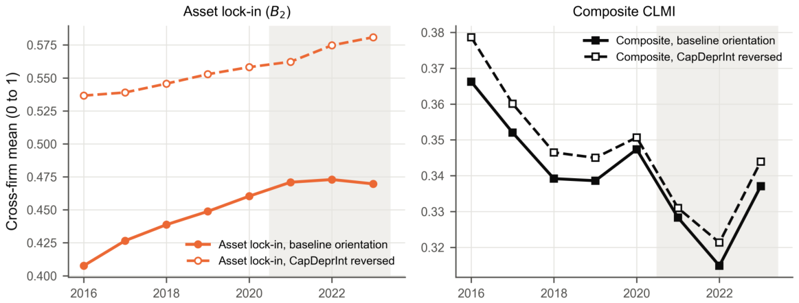
Appendix B. Derivation of the Discrete-Time Panel VAR from the Continuous-Time Matrix ODE
Appendix B.1. Full Derivation from the Causal Loop Diagram to the Discrete-Time Panel Equation
Appendix B.1.1. Step 1: Continuous-Time ODE in Vector Form
Reading directly from the CLD, the state evolution along four dimensions is:
where
Matrix : Self-Feedback and Cross-Feedback
The diagonal elements originate from self-feedback loops S1–S4; the off-diagonal elements originate from cross-feedback loops D1–D12. Reading element by element from the CLD:
The CLD supplies candidate directions, but estimation does not impose positive signs. For the off-diagonal elements, a positive would support the hypothesized reinforcing path and a negative estimate would identify a balancing path. For the diagonal, persistence is evaluated in discrete time: indicates positive state dependence with mean reversion, even though the Euler mapping is negative. It would therefore be incorrect to require every element of to exceed zero.
Matrix : Exogenous Drivers
Reading element by element from the CLD:
The entries of are likewise estimated without sign restrictions. The same input can operate through competing mechanisms, for example, a higher energy price can intensify use of sunk technology while strengthening governance attention, and capital expenditure can renew carbon-intensive or low-carbon assets. The empirical sign, therefore, determines whether an input deepens or eases each lock-in state.
Appendix B.1.2. Step 2: Forward Euler Discretization
Discretization Formula
With annual data , substituting into the continuous ODE:
Discrete System Matrix
Let
Incorporating the panel structure (firm fixed effects and idiosyncratic disturbance ):
where (firms), .
Appendix B.1.3. Step 3: Expansion into Below Four Scalar Equations
- First equation: (Technological Lock-in)
- Second equation: (Asset Lock-in)
- Third equation: (Institutional Lock-in)
- Forth equation: (Market Lock-in)
Table A8 reports the continuous-time system matrix and the eigenvalues used to verify dynamic stability.
Table A8.
Dynamic stability verification of the estimated continuous- and discrete-time carbon lock-in systems.
Figure A2 traces the responses implied by the estimated feedback matrix to a shock of 0.1 in each lock-in state; filled markers indicate horizons at which the band between the 5th and 95th percentiles of 499 firm-cluster bootstrap replications excludes zero. Own responses dominate every column. The two largest cross-dimensional responses, of institutional lock-in to a technological shock ( after one year) and of asset lock-in to a market shock (), are less than half of the corresponding own responses in the same year and about one-sixth of the cumulative own responses, and they fade within three years. Table A9 reports the system under alternative estimators, a second lag, alternative samples, and fit diagnostics (Section 5.2).
Figure A2.
Impulse responses of the four lock-in states. Columns give the shocked state (a one-time shock of 0.1) and rows the responding state; horizontal axes count years after the shock. Lines are point estimates from in Table 5; filled markers indicate that the band between the 5th and 95th percentiles of 499 firm-cluster bootstrap replications excludes zero, hollow markers that it does not.
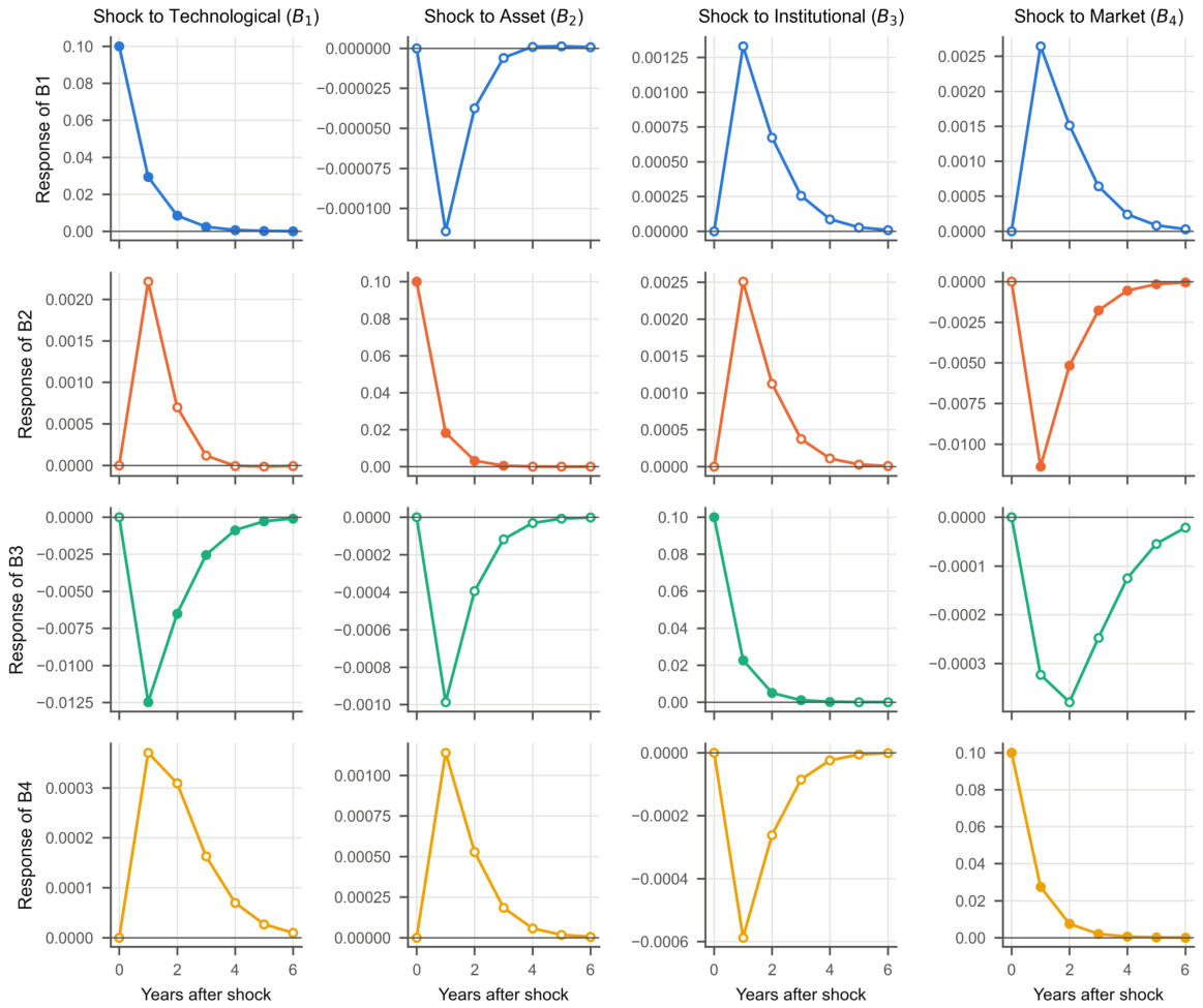
Table A9.
Further robustness of the panel feedback system: estimators, lag structure, influential observations, and fit.
Appendix C. Scenario Design and Sensitivity Results
Table A10 specifies the exogenous paths used in the scenario simulations, Table A11 and Table A12 report the gradient sensitivity analysis, and Figure A3, Figure A4 and Figure A5 display the dimension-level projections, terminal-year deviations, and tornado diagrams. Table A13 repeats the combined scenario with the transition matrix of each alternative estimator and index construction.
Table A10.
Exogenous input paths in the counterfactual scenarios, 2024–2035.
Figure A3.
Dimension-level carbon lock-in projections under counterfactual policy scenarios, 2024–2035. Each panel shows the historical cross-firm mean (2016–2023) and six projections from , starting from the baseline steady state. S0 holds all exogenous inputs at their 2016–2023 sample means; S1 and S2 shift the coal price permanently by and ; S3 and S4 shift capital expenditure by and ; S5 applies shocks to both. Pollution-control investment and energy intensity stay at their sample means. The dashed vertical line marks the start of the projection.
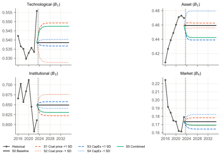
Figure A4.
Percentage deviations from the baseline scenario in 2035 across lock-in dimensions. Bars show the deviation of each lock-in dimension and of the equal-weighted index from S0 in 2035 under scenarios S1–S5 (Table A10). Positive values indicate deeper lock-in than the baseline; negative values indicate less lock-in.
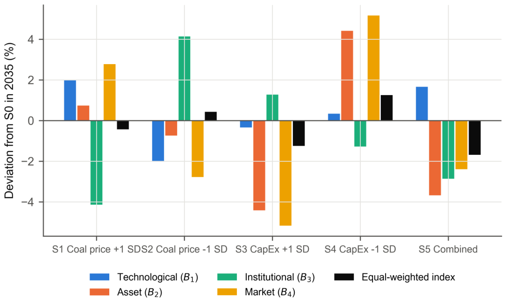
Table A11.
Gradient sensitivity of the lock-in dimensions to symmetric shocks in the exogenous drivers.
Table A12.
Symmetric central-difference elasticities of endogenous lock-in dimensions with respect to exogenous policy drivers.
Figure A5.
Sensitivity of the lock-in dimensions in 2035 to permanent shocks of different size. Each panel reports the deviation of one dimension from S0 in 2035 () induced by a permanent shock of , , , or to a single input, with darker shading for larger shocks; the upper row shocks the coal price and the lower row capital expenditure. All other inputs stay at their sample means. Deviations scale linearly with shock size because the state equation is linear.
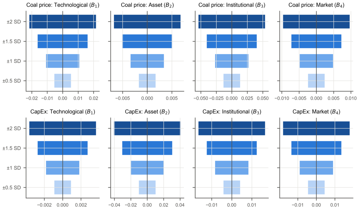
Table A13.
Sensitivity of the combined-lever scenario to the estimated system.
Appendix D. Fuzzy-Set QCA: Calibration, Necessity, Truth Tables, and Robustness
This appendix reports the calibration anchors (Table A14), the necessity analysis (Table A15), the truth tables and Boolean minimization for each period and condition group (Table A16, Table A17, Table A18 and Table A19), and the robustness of the configurational solutions (Table A20 and Table A21). The financing condition is the KZ index, and a truth-table row is coded as leading to high lock-in when its consistency is at least 0.75 and its PRI at least 0.50.
Table A14.
Fuzzy-set calibration anchors for the outcome and condition variables across policy periods.
Table A15.
Necessity analysis of individual conditions for high corporate carbon lock-in across policy periods.
Table A16.
Truth table and boolean minimization for high corporate carbon lock-in under micro-level conditions in the pre-policy period, 2016–2019.
Table A17.
Truth table and boolean minimization for high corporate carbon lock-in under micro-level conditions in the post-policy period, 2020–2023.
Table A18.
Truth table and boolean minimization for high corporate carbon lock-in under macro-level conditions in the pre-policy period, 2016–2019.
Table A19.
Truth table and boolean minimization for high corporate carbon lock-in under macro-level conditions in the post-policy period, 2020–2023.
Table A20.
Robustness of configurational solutions across alternative fsQCA calibration and threshold specifications.
Table A21.
Condition stability across alternative fsQCA specifications.
Appendix E. Robustness of the Carbon-Market Estimates
Table A22 reports the difference-in-differences estimates of Table 8, Panel A, under alternative samples, trends, treatment dates, and control groups. Table A23 reports the placebo assignment of coverage to each of the eight sectors and the Conley–Taber draws, and Table A24 repeats the financing-constraint split of Table 8, Panel B, with the SA index, the cost of debt, and firm age.
Table A22.
Robustness of the carbon-market difference-in-differences estimates.
Table A23.
Inference for a single treated sector: placebo coverage of each sector and Conley–Taber draws.
Table A24.
Carbon-market coverage by financing constraints: alternative measures.
Appendix F. Supplementary Descriptive Figures
Figure A6 plots the annual means of the nine CLMI sub-indicators, and Figure A7 reports their pairwise correlations with the dimensional indices and the composite index.
Figure A6.
Annual means of the CLMI sub-indicators in their original units, 2016–2023. Each panel plots the cross-firm annual mean (333 firms) before normalization and before the four negatively oriented indicators (GreenPat, RdInt, EnvReg, InstCompl) are reversed. InstCompl is the count of carbon-related words in annual and CSR reports; EnvReg is the share of environment-related keywords in provincial government work reports. The shaded period follows the start of trading in the national emissions trading scheme (July 2021). Note the narrow vertical range of the high-carbon energy share.
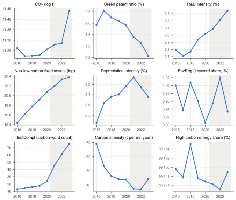
Figure A7.
Pearson correlation matrix of the CLMI sub-indicators, dimensional indices, and the composite and additive indices. Sub-indicators are min–max normalized and oriented so that higher values mean deeper lock-in (2664 firm-years). *, **, and *** denote correlations significant at the 10%, 5%, and 1% levels, respectively.
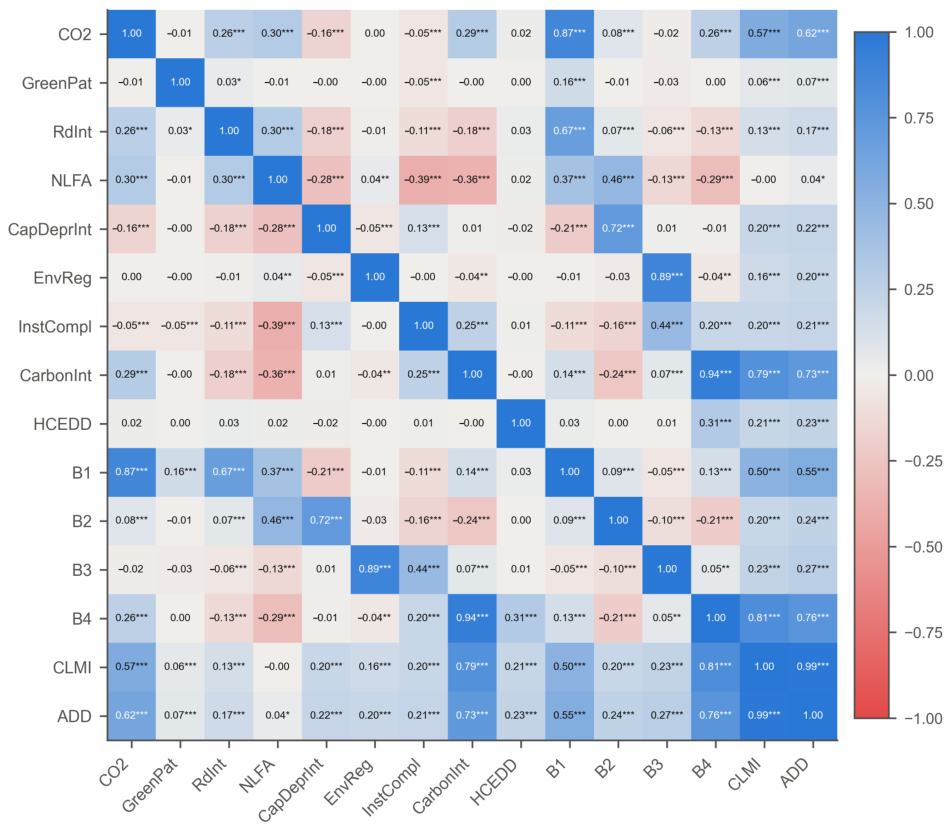
References
- Aghion, P., Dechezleprêtre, A., Hémous, D., Martin, R., & Van Reenen, J. (2016). Carbon taxes, path dependency, and directed technical change: Evidence from the auto industry. Journal of Political Economy, 124(1), 1–51. [Google Scholar] [CrossRef] [Scilit]
- Anderson, T. W., & Hsiao, C. (1982). Formulation and estimation of dynamic models using panel data. Journal of Econometrics, 18(1), 47–82. [Google Scholar] [CrossRef] [Scilit]
- Arellano, M., & Bond, S. (1991). Some tests of specification for panel data: Monte Carlo evidence and an application to employment equations. Review of Economic Studies, 58(2), 277–297. [Google Scholar] [CrossRef] [Scilit]
- Barbieri, N., Marzucchi, A., & Rizzo, U. (2020). Knowledge sources and impacts on subsequent inventions: Do green technologies differ from non-green ones? Research Policy, 49(2), 103901. [Google Scholar] [CrossRef] [Scilit]
- Bartram, S. M., Hou, K., & Kim, S. (2022). Real effects of climate policy: Financial constraints and spillovers. Journal of Financial Economics, 143(2), 668–696. [Google Scholar] [CrossRef] [Scilit]
- Bolton, P., & Kacperczyk, M. (2021). Do investors care about carbon risk? Journal of Financial Economics, 142(2), 517–549. [Google Scholar] [CrossRef] [Scilit]
- Calel, R., & Dechezleprêtre, A. (2016). Environmental policy and directed technological change: Evidence from the European carbon market. Review of Economics and Statistics, 98(1), 173–191. [Google Scholar] [CrossRef] [Scilit]
- Cao, J., Ho, M. S., Ma, R., & Teng, F. (2021). When carbon emission trading meets a regulated industry: Evidence from the electricity sector of China. Journal of Public Economics, 200, 104470. [Google Scholar] [CrossRef] [Scilit]
- Chen, Z., Kahn, M. E., Liu, Y., & Wang, Z. (2018). The consequences of spatially differentiated water pollution regulation in China. Journal of Environmental Economics and Management, 88, 468–485. [Google Scholar] [CrossRef] [Scilit]
- Conley, T. G., & Taber, C. R. (2011). Inference with “difference in differences” with a small number of policy changes. Review of Economics and Statistics, 93(1), 113–125. [Google Scholar] [CrossRef] [Scilit]
- Cui, J., Wang, C., Zhang, J., & Zheng, Y. (2021). The effectiveness of China’s regional carbon market pilots in reducing firm emissions. Proceedings of the National Academy of Sciences the United States of America, 118(52), e2109912118. [Google Scholar] [CrossRef] [Scilit]
- Dhaene, G., & Jochmans, K. (2015). Split-panel jackknife estimation of fixed-effect models. Review of Economic Studies, 82(3), 991–1030. [Google Scholar] [CrossRef] [Scilit]
- Duşa, A. (2019). QCA with R: A comprehensive resource. Springer. [Google Scholar] [CrossRef] [Scilit]
- Erickson, P., Kartha, S., Lazarus, M., & Tempest, K. (2015). Assessing carbon lock-in. Environmental Research Letters, 10(8), 084023. [Google Scholar] [CrossRef] [Scilit]
- Fiss, P. C. (2011). Building better causal theories: A fuzzy set approach to typologies in organization research. Academy of Management Journal, 54(2), 393–420. [Google Scholar] [CrossRef] [Scilit]
- Fouquet, R. (2016). Path dependence in energy systems and economic development. Nature Energy, 1(8), 16098. [Google Scholar] [CrossRef] [Scilit]
- Geels, F. W. (2014). Regime resistance against low-carbon transitions: Introducing politics and power into the multi-level perspective. Theory, Culture & Society, 31(5), 21–40. [Google Scholar] [CrossRef] [Scilit]
- Greckhamer, T., Furnari, S., Fiss, P. C., & Aguilera, R. V. (2018). Studying configurations with qualitative comparative analysis: Best practices in strategy and organization research. Strategic Organization, 16(4), 482–495. [Google Scholar] [CrossRef] [Scilit]
- Hadlock, C. J., & Pierce, J. R. (2010). New evidence on measuring financial constraints: Moving beyond the KZ index. Review of Financial Studies, 23(5), 1909–1940. [Google Scholar] [CrossRef] [Scilit]
- Hart, S. L. (1995). A natural-resource-based view of the firm. Academy of Management Review, 20(4), 986–1014. [Google Scholar] [CrossRef] [Scilit]
- Hart, S. L., & Dowell, G. (2011). A natural-resource-based view of the firm: Fifteen years after. Journal of Management, 37(5), 1464–1479. [Google Scholar] [CrossRef] [Scilit]
- Kaplan, S. N., & Zingales, L. (1997). Do investment-cash flow sensitivities provide useful measures of financing constraints? Quarterly Journal of Economics, 112(1), 169–215. [Google Scholar] [CrossRef] [Scilit]
- Klitkou, A., Bolwig, S., Hansen, T., & Wessberg, N. (2015). The role of lock-in mechanisms in transition processes: The case of energy for road transport. Environmental Innovation and Societal Transitions, 16, 22–37. [Google Scholar] [CrossRef] [Scilit]
- Krueger, P., Sautner, Z., & Starks, L. T. (2020). The importance of climate risks for institutional investors. Review of Financial Studies, 33(3), 1067–1111. [Google Scholar] [CrossRef] [Scilit]
- Liu, L. (2026). Impact of firm ESG performance on cost of debt: Insights from the Chinese bond market. Macroeconomics and Finance in Emerging Market Economies, 19(3), 601–620. [Google Scholar] [CrossRef] [Scilit]
- Liu, Z., Deng, Z., Davis, S. J., Giron, C., & Ciais, P. (2022a). Monitoring global carbon emissions in 2021. Nature Reviews Earth & Environment, 3(4), 217–219. [Google Scholar] [CrossRef] [Scilit]
- Liu, Z., Deng, Z., He, G., Wang, H., Zhang, X., Lin, J., Qi, Y., & Liang, X. (2022b). Challenges and opportunities for carbon neutrality in China. Nature Reviews Earth & Environment, 3(2), 141–155. [Google Scholar] [CrossRef] [Scilit]
- Mallapaty, S. (2020). How China could be carbon neutral by mid-century. Nature, 586(7830), 482–483. [Google Scholar] [CrossRef] [Scilit]
- Markard, J., Raven, R., & Truffer, B. (2012). Sustainability transitions: An emerging field of research and its prospects. Research Policy, 41(6), 955–967. [Google Scholar] [CrossRef] [Scilit]
- Marquis, C., & Qian, C. (2014). Corporate social responsibility reporting in China: Symbol or substance? Organization Science, 25(1), 127–148. [Google Scholar] [CrossRef] [Scilit]
- Nickell, S. (1981). Biases in dynamic models with fixed effects. Econometrica, 49(6), 1417–1426. [Google Scholar] [CrossRef] [Scilit]
- Papachristos, G. (2017). Diversity in technology competition: The link between platforms and sociotechnical transitions. Renewable and Sustainable Energy Reviews, 73, 291–306. [Google Scholar] [CrossRef] [Scilit]
- Pfeiffer, A., Millar, R., Hepburn, C., & Beinhocker, E. (2016). The ‘2 °C capital stock’ for electricity generation: Committed cumulative carbon emissions from the electricity generation sector and the transition to a green economy. Applied Energy, 179, 1395–1408. [Google Scholar] [CrossRef] [Scilit]
- Ragin, C. C. (2008). Redesigning social inquiry: Fuzzy sets and beyond. University of Chicago Press. [Google Scholar] [CrossRef] [Scilit]
- Rosenbloom, D., Markard, J., Geels, F. W., & Fuenfschilling, L. (2020). Why carbon pricing is not sufficient to mitigate climate change—And how “sustainability transition policy” can help. Proceedings of the National Academy of Sciences the United States of America, 117(16), 8664–8668. [Google Scholar] [CrossRef] [Scilit]
- Schneider, C. Q., & Wagemann, C. (2012). Set-theoretic methods for the social sciences: A guide to qualitative comparative analysis. Cambridge University Press. [Google Scholar] [CrossRef] [Scilit]
- Seto, K. C., Davis, S. J., Mitchell, R. B., Stokes, E. C., Unruh, G., & Ürge-Vorsatz, D. (2016). Carbon lock-in: Types, causes, and policy implications. Annual Review of Environment and Resources, 41, 425–452. [Google Scholar] [CrossRef] [Scilit]
- Sterman, J. D. (2000). Business dynamics: Systems thinking and modeling for a complex world. McGraw-Hill. [Google Scholar]
- Tan, R., Cai, Q., & Pan, L. (2024). Faking for fortune: Emissions trading schemes and corporate greenwashing in China. Energy Economics, 130, 107319. [Google Scholar] [CrossRef] [Scilit]
- Tong, D., Zhang, Q., Zheng, Y., Caldeira, K., Shearer, C., Hong, C., Qin, Y., & Davis, S. J. (2019). Committed emissions from existing energy infrastructure jeopardize 1.5 °C climate target. Nature, 572(7769), 373–377. [Google Scholar] [CrossRef] [Scilit]
- Unruh, G. C. (2000). Understanding carbon lock-in. Energy Policy, 28(12), 817–830. [Google Scholar] [CrossRef] [Scilit]
- Unruh, G. C. (2002). Escaping carbon lock-in. Energy Policy, 30(4), 317–325. [Google Scholar] [CrossRef] [Scilit]
- Unruh, G. C. (2019). The real stranded assets of carbon lock-in. One Earth, 1(4), 399–401. [Google Scholar] [CrossRef] [Scilit]
- Wei, Z., Zeng, A., & Li, B. (2014). Financial ecological environment and corporate financial constraints: Evidence from Chinese listed companies. Accounting Research, (5), 73–80. (In Chinese) [Google Scholar]
- Wooldridge, J. M. (2010). Econometric analysis of cross section and panel data (2nd ed.). MIT Press. [Google Scholar]
- Xu, Q., & Kim, T. (2022). Financial constraints and corporate environmental policies. Review of Financial Studies, 35(2), 576–635. [Google Scholar] [CrossRef] [Scilit]
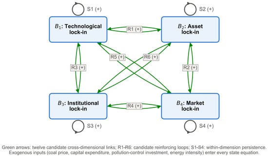
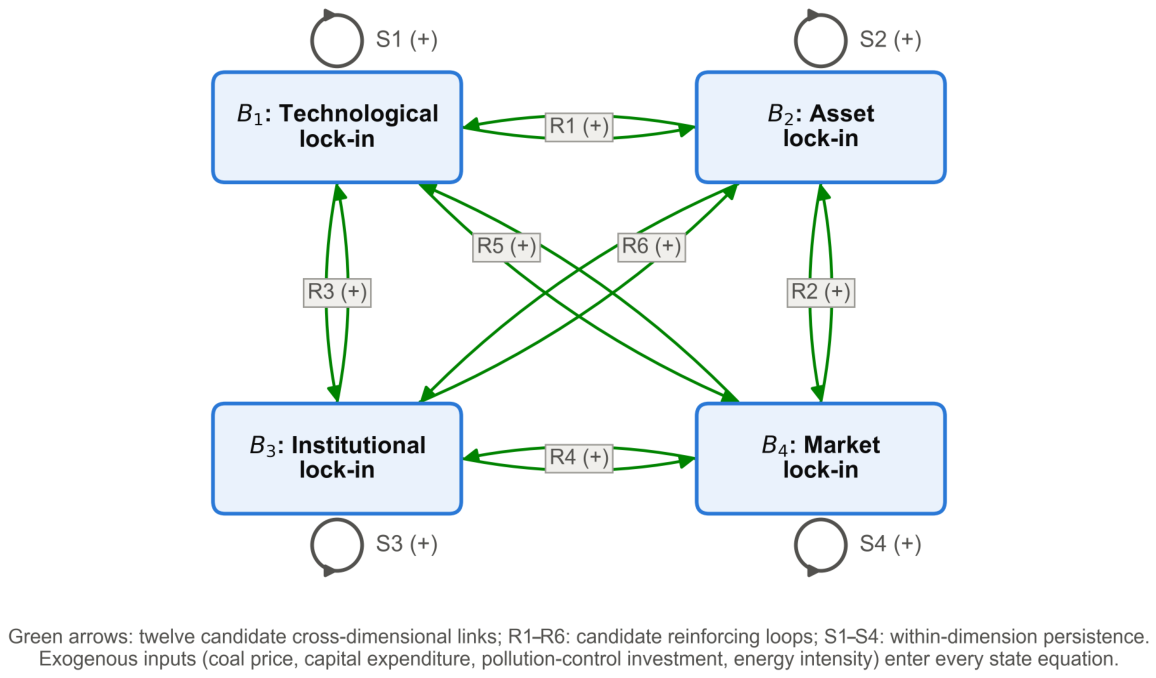
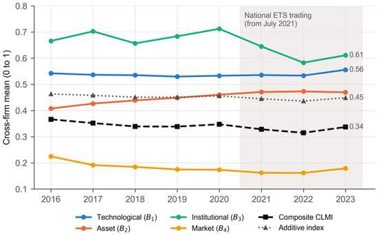
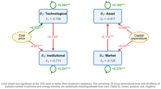
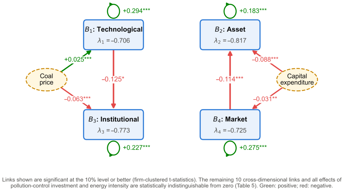
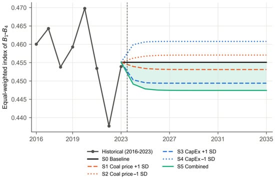
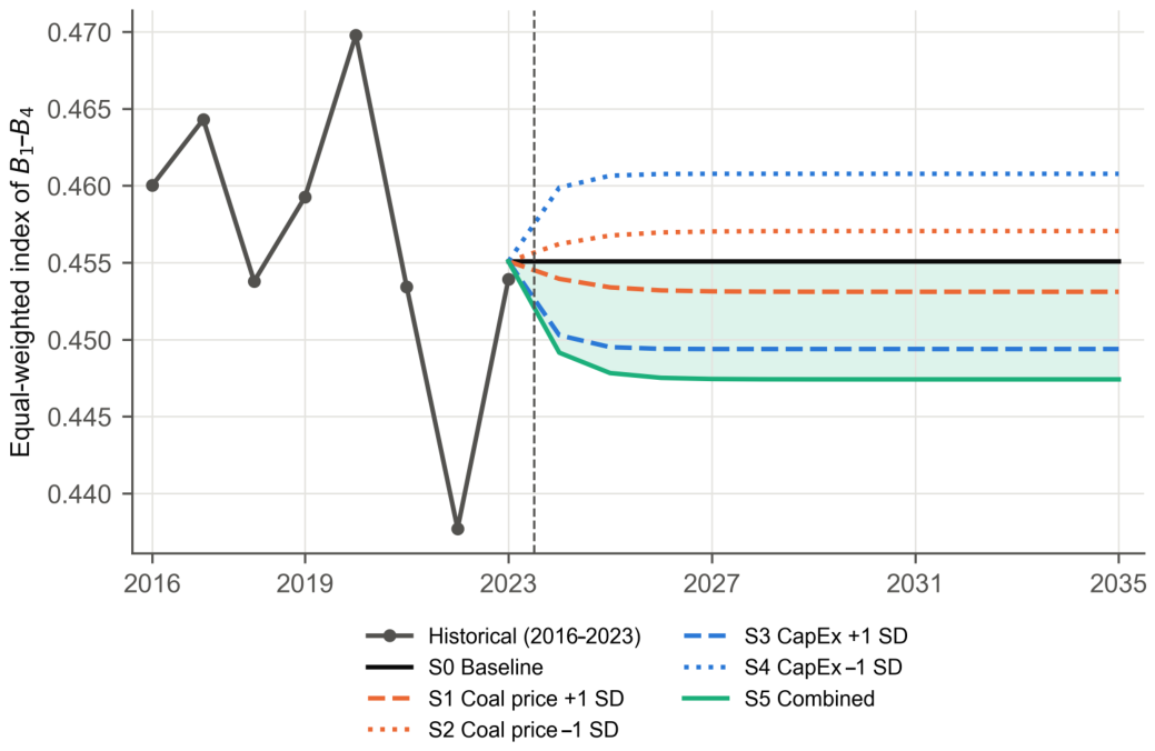
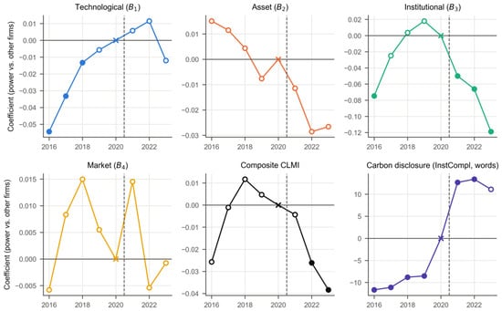
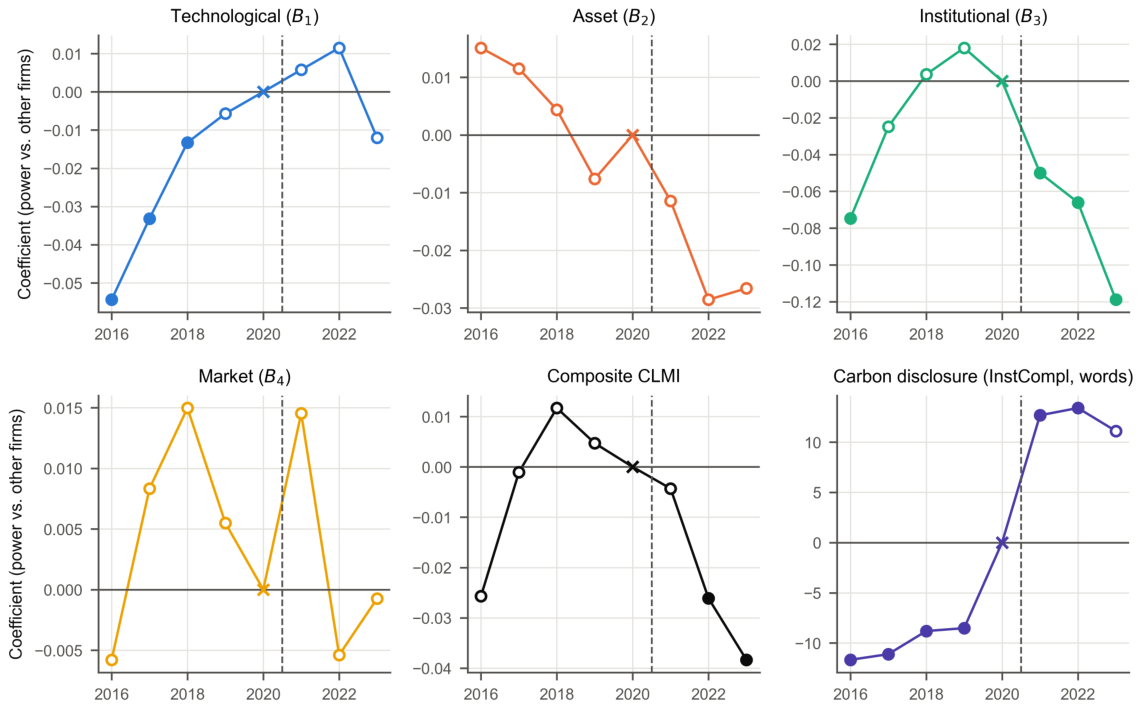
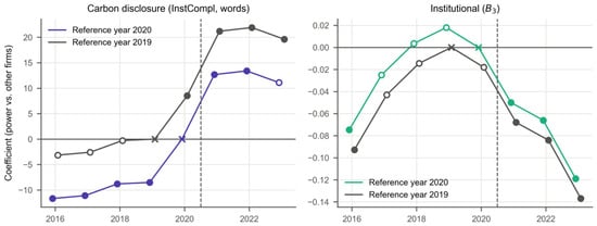
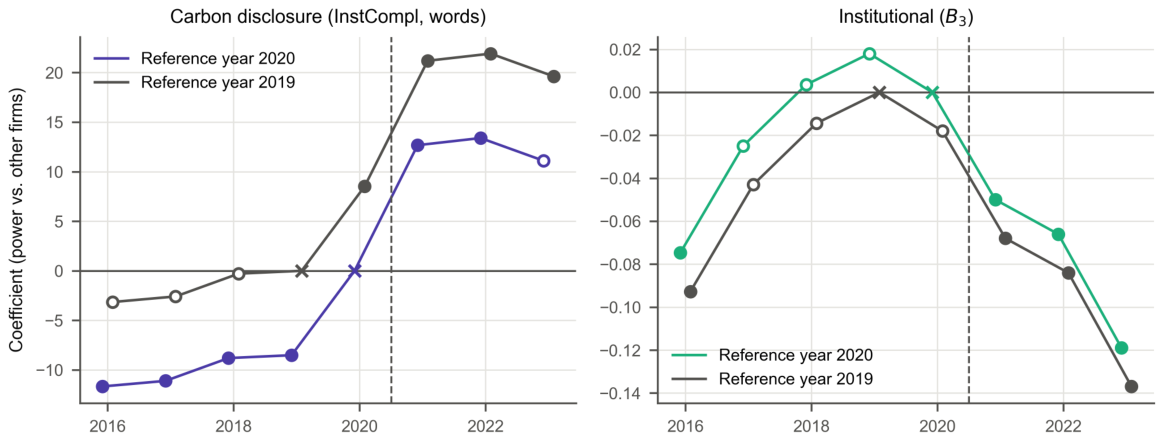

Disclaimer/Publisher’s Note: The statements, opinions and data contained in all publications are solely those of the individual author(s) and contributor(s) and not of MDPI and/or the editor(s). MDPI and/or the editor(s) disclaim responsibility for any injury to people or property resulting from any ideas, methods, instructions or products referred to in the content. |
© 2026 by the authors. Licensee MDPI, Basel, Switzerland. This article is an open access article distributed under the terms and conditions of the Creative Commons Attribution (CC BY) license.