


Abstract
This study assesses machine learning’s incremental forecasting value for the Borsa Istanbul Tourism Index through directional, probabilistic, and intraday economic evaluations. Twenty-three market-based predictors from daily 2010–2026 data were used at 1644 forecast origins in 2020–July 2026. Hyperparameters were selected using outcomes realized before 2020, and models were refitted quarterly. Logistic regression, random forest, XGBoost, and long short-term memory networks were compared with majority, historical-prevalence, directional-persistence, and first-order probabilistic-persistence benchmarks. Paired circular moving-block bootstrap inference addressed serial dependence and multiple comparisons. Inference was conditional on selected configurations and fitted models, excluding uncertainty from repeated hyperparameter selection and model fitting. Directional persistence achieved the highest Matthews correlation coefficient (MCC), 0.110, versus approximately 0.088 for logistic regression and random forest. No fitted model established MCC superiority over persistence. XGBoost’s Brier score was 0.24610, versus 0.24888 for historical prevalence and 0.24738 for probabilistic persistence; primary adjusted comparisons did not establish superiority over either benchmark. Separately selected intraday configurations aligned forecasts with holding periods. Economic outcomes varied across periods, with uncertain excess returns over interest-bearing cash. Distributed outputs support numerical verification; full reproduction requires authorized source data and the documented estimation environment.
1. Introduction
Tourism is sensitive to pandemics, geopolitical crises, natural disasters, and exchange-rate changes that disrupt demand and revenues (Gössling et al., 2021). These shocks affect expectations for listed tourism companies. The Borsa Istanbul (BIST) Tourism Index offers a financial setting for testing whether past market information predicts short-horizon movements. The forecasting question concerns observable investment signals.
The pandemic intensified interest in the financial performance of tourism firms. Wu et al. (2021) documented nonlinear responses of Chinese-listed tourism companies to pandemic news and government interventions. Using 40 international tourism and hospitality stock indices, Liu et al. (2023) found substantial changes in connectedness following the pandemic’s onset. Sahiner et al. (2026) examined changes in return and volatility spillovers during the crisis and recovery. These findings motivate attention to temporal variation in forecasting performance.
Studies of Turkey also document this financial sensitivity. Katircioglu and Katircioglu (2023) showed that tourism stock returns are closely related to broader business and financial conditions. Helhel and Helhel (2026) examined Borsa Istanbul tourism companies from 2012 to 2025 in relation to economic and geopolitical risks. They identified leverage and growth as important factors and highlighted vulnerability to successive crises. These studies primarily explain sectoral risk. They do not directly test whether available data can predict the next day’s market direction.
Direct forecasting evidence is available for the BIST Tourism Index (XTRZM). Gülay et al. (2023) compared autoregressive integrated moving average models and convolutional neural networks for index-level forecasts using percentage prediction errors. The present study extends this sector-specific evidence by examining next-session direction and the incremental value of fitted models over explicit forecasting rules. Its evaluation links the timing of available information to directional classification, probability scoring, and a separately defined intraday economic objective.
Predictability is a longstanding question in finance. The efficient market hypothesis holds that publicly available information is reflected in prices. This limits persistent gains from past prices alone (Fama, 1970). Machine learning may identify directional signals by capturing complex nonlinear relationships. Patel et al. (2015) compared four classifiers and found that the trend-based preprocessing of technical indicators improved directional prediction. Ballings et al. (2015) benchmarked ensemble methods against single classifiers, with random forest performing best. Fischer and Krauss (2018) found that long short-term memory (LSTM) networks outperformed methods without memory. Gu et al. (2020) reported improved risk-premium estimates in asset pricing.
Several design choices can inflate apparent forecasting performance. These include selecting hyperparameters using evaluation-period outcomes, relying on accuracy despite class imbalance, omitting transaction costs, and overlooking temporal variation. A model’s performance also depends on the benchmark against which incremental value is assessed. Constant probabilities provide a limited test when a simple transition model can exploit directional dependence. For XTRZM, evidence based on explicit directional and probabilistic benchmarks remains comparatively limited.
Direction forecasting and return estimation address different objectives. Daily returns contain substantial noise, while classification evaluates the sign of a movement without estimating its magnitude. However, a correct directional forecast need not imply an economically useful trade. Probability scores, threshold-based classification measures, and returns over a specified holding period must therefore be evaluated separately.
The research question is whether machine learning adds out-of-sample predictive value beyond simple historical forecasting rules for the next-day direction of the BIST Tourism Index. The study contributes a sector-specific empirical assessment that brings directional and probabilistic benchmarks into a common temporal evaluation. First-order transition probabilities test whether fitted probability forecasts add information beyond simple directional dependence. Separately selected intraday models align the economic exercise with its forecast target and holding period. Calendar-period and specification checks document how the findings vary across time and modeling choices. The distributed forecasts, return paths, and verification code support direct examination of these comparisons. Together, these elements provide an empirical reference for assessing incremental forecasting value in tourism finance.
2. Materials and Methods
2.1. Data and Sample
The source archive contained 4161 daily observations from 4 January 2010 to 31 July 2026. It included opening, high, low, and closing prices and provider-reported volume from Investing.com’s BIST Tourism historical-data page (Investing.com, n.d.). XTRZM is an uncapped, market-capitalization-weighted price index denominated in Turkish lira (Borsa İstanbul, n.d.). Its price-index construction excludes dividend reinvestment (Borsa İstanbul, 2026). The vendor’s volume field was treated as an activity measure because its unit and aggregation were not independently established as tradable index volume.
Two records were excluded. 1 January 2013 was an official holiday associated with a reported 9899.38% change. 8 February 2023 was excluded because Borsa İstanbul suspended equity trading following the earthquakes and canceled that day’s transactions (Borsa İstanbul, 2023). The cleaned series contained 4159 observations. Removing 20 feature-warm-up observations and the final observation without a future outcome yielded 4138 model-ready forecast origins. Fixed rolling indicators required at most 20 observations, whereas recursive indicators used preceding history. The selected LSTM window contained 40 consecutive model-ready predictor observations. The first 39 endpoints lacked complete sequences. All models nevertheless shared the same evaluation origins.
2.2. Target Variable and Features
Let Ct denote the index closing value on session t. The daily logarithmic return is defined in Equation (1).
The primary binary target records whether the following session’s close exceeds the current close. It is forecast using information available at the close of session t, as defined in Equation (2).
Unchanged next-session closing prices were assigned to the non-upward class. All 23 predictors used information available by the origin close. The designated return group contained the current daily log return, its four lags, and cumulative returns over 5, 10, and 20 sessions. The volatility group contained rolling return volatility over the same horizons. The technical and volume group contained the overnight gap, intraday return, log high–low range, closing-price location, normalized average true range, and relative strength index (Wilder, 1978). It also included normalized moving average convergence divergence (MACD) and its signal line, Bollinger %B and bandwidth (Bollinger, 2001), log volume changes, and standardized log volume. Table S1 provides definitions. Scaling parameters were estimated exclusively from the relevant training observations. The groups describe column assignments with overlapping information. In particular, the overnight gap plus the intraday log return exactly equals the current close-to-close log return.
2.3. Temporal Design and Hyperparameter Selection
Hyperparameter selection used only origins whose next-record outcomes were realized by 31 December 2019. The final eligible origin was 30 December 2019, yielding 2493 tuning observations. Four expanding outer folds used 252-observation validation windows and a one-observation purge gap (Bergmeir & Benítez, 2012). Fixed-seed candidate sampling evaluated mean validation MCC (Bergstra & Bengio, 2012). Configurations less than 0.005 below the best mean MCC were ranked lexicographically by their available structural parameters. The ordering was tree count, maximum depth, hidden width, layer count, and sequence length. Unrestricted tree depth ranked above finite depth. Unranked parameters did not affect this structural preference. Equal structural ranks retained the higher MCC. Logistic-regression C was unranked. Accordingly, C = 10 was selected because its mean MCC of 0.03437 exceeded 0.03241 for C = 1. Table S2 specifies the rule for each model class and the selected configurations.
Evaluation covered 1644 forecast origins from 2 January 2020 to 30 July 2026, with outcomes realized from 3 January 2020 to 31 July 2026. Each quarterly fit occurred after the close of the quarter’s first evaluation origin. Eligible training origins preceded that information date and their outcomes had to be realized by that close. The current predictors then produced the next-session forecast. Hyperparameters remained fixed across 27 expanding quarterly fits. Classification subperiods were defined by forecast-origin dates as 2020–2021, 2022–2023, and 2024–July 2026. Stored forecasts identify both the fitting information date and the last training-outcome date.
2.4. Models Compared
Four benchmarks addressed distinct comparisons. Majority predicted the dominant training class, re-estimated at each quarterly fitting date. The upward class remained dominant at all 27 fits. Historical prevalence assigned the training proportion of upward outcomes, re-estimated at each quarterly fitting date. This probability was constant within a quarter and varied across quarters. Its pooled ROC-AUC therefore need not equal 0.500. Directional persistence repeated the current close-to-close sign. Probabilistic persistence estimated the first-order conditional probability of the next direction given the current direction. It used the same eligible training endpoints and quarterly information cutoffs. Current zero returns belonged to the non-upward state. Transition estimates were unsmoothed. An empty conditioning cell would use the training prevalence, although no such cell occurred. All probabilities were fixed between quarterly fits. Logistic regression used L2 regularization with C in {0.1, 1, 10}. Random forest evaluated 16 sampled configurations (Breiman, 2001), XGBoost evaluated 20 (Chen & Guestrin, 2016), and LSTM evaluated eight (Hochreiter & Schmidhuber, 1997; Kingma & Ba, 2015). The primary threshold was 0.50 and was not selected using evaluation outcomes. A quarterly audit confirms ROC-AUC = 0.500 within every evaluation quarter for historical prevalence. Its pooled value reflects updating across quarters.
Early stopping was nested within each outer training set. Its final 15% formed an inner validation tail separated from the fitting prefix by one observation. Scaling for this stage used the prefix only. XGBoost used at most 600 boosting rounds and a stopping patience of 30 rounds. LSTM used at most 80 Adam epochs and a patience of eight epochs. The selected number of rounds or epochs then determined a fresh fit on the full outer training set, with LSTM scaling re-estimated from that set. Quarterly estimation repeated this procedure using only outcomes available at the information date. Outer validation outcomes did not determine stopping times. Sequence models required complete predictor windows.
2.5. Evaluation Metrics and Statistical Inference
The primary performance metrics were MCC and balanced accuracy (BA). MCC provides a more informative assessment than accuracy or the F1 score when binary classes are imbalanced (Chicco & Jurman, 2020; Matthews, 1975). Equations (3) and (4) define these metrics using true positives (TPs), true negatives (TNs), false positives (FPs), and false negatives (FNs).
Accuracy, ROC-AUC, and the Brier score complemented MCC and balanced accuracy (Brier, 1950). Undefined MCC denominators were assigned a value of zero. Uncertainty was assessed using a joint circular moving-block bootstrap with 2000 fixed-seed draws. Identical index draws resampled each model’s forecasts and the realized outcomes, preserving paired comparisons. Blocks wrapped around the evaluation series. The primary block length was ten observations. Lengths of five and twenty assessed sensitivity. Percentile intervals were calculated at the 95% level. This fixed-length procedure differs from the random-length stationary bootstrap (Künsch, 1989; Politis & Romano, 1994).
Inference evaluates the recorded forecast paths conditional on the selected configurations and fitted models. Shared block draws preserve pairing and local dependence. Hyperparameter selection, early stopping, and quarterly fitting remain fixed within the bootstrap. The intervals therefore quantify uncertainty in comparisons between these forecast paths and do not include uncertainty from repeating the complete estimation procedure (West, 1996). Seed replications, the controlled LSTM label experiment, and the intraday configuration comparison examine additional, specified sources of variability.
Comparative conclusions used paired bootstrap differences. Two-sided p-values compared each observed difference with its null-centered bootstrap distribution using a plus-one finite-simulation adjustment. For each target and classification metric, Holm correction covered 14 comparisons (Holm, 1979). These comprised four fitted models against majority and directional persistence, plus six fitted-model pairs. The Brier family covered eight comparisons between the four fitted models and the two probability benchmarks. Each descriptive probability subperiod used the same eight-comparison family. Difference intervals were nominal. Adjusted p-values determined multiplicity-controlled claims within the stated families, and subperiod results were exploratory. Conventional Pesaran–Timmermann and McNemar tests did not determine superiority claims because they do not explicitly adjust for temporal dependence (McNemar, 1947; Pesaran & Timmermann, 1992). The correction applies to these comparison families rather than every analytical choice in the retrospective design.
Data-treatment checks retained the suspension record or excluded flat close-to-close training outcomes while holding hyperparameters fixed. Suspension-record comparisons matched origin dates, realized outcome dates, and labels. Changed outcomes were excluded explicitly. The flat-label check retained the complete predictor timeline and removed only ineligible supervised training endpoints. All 40-observation LSTM windows therefore retained their original consecutive predictors. Twenty-one pre-2020 training endpoints were excluded, while all 1644 evaluation origins remained. A reference LSTM retaining all training labels was fitted in the same computational environment as the excluded-label model. This design separates label eligibility from platform-dependent training variation. Table S8 distinguishes the controlled reference from the saved primary LSTM forecasts.
2.6. Training-Seed and Feature-Group Checks
Random forest, XGBoost, and LSTM used three fixed base seeds, 20260801, 20260802, and 20260803. Model and quarterly offsets were deterministic, and hyperparameters were unchanged. Logistic-regression ablations separately removed the explicitly designated return, volatility, and technical/volume columns, retaining the same observations and regularization setting. Paired MCC differences compared each refitted reduced specification with the full specification. Removing the designated return columns retains current-return information through the exact identity return_lag_1 = overnight_gap + intraday_return. Both right-hand terms remain in the technical group. These comparisons assess predictive sensitivity to column composition under fixed regularization. The overlap prevents them from isolating the unique contribution of return information or causal predictor effects.
Two additional sensitivities retained the primary hyperparameters and evaluation origins. For each fitted model, a threshold from 0.05 to 0.95 in steps of 0.01 maximized pooled MCC across the four purged pre-2020 validation folds. Exact ties favored the threshold closest to 0.50, followed by the lower value. Only outcomes realized by December 2019 entered this selection. The volume-only check removed log_volume_change and volume_zscore20. It retained the other 21 predictors and repeated the same quarterly fitting and seed schedule. Each sensitivity used the existing 14-comparison MCC family separately (Tables S11 and S12).
2.7. Hypothetical Economic Exercise
A hypothetical long/cash strategy entered at the next session’s open and exited at its close after an upward forecast. The primary close-to-close and open-to-close signs differed at 189 of 1644 origins (11.50%). Economic evaluation therefore used a separate next-session open-to-close target. Intraday-specific hyperparameters used only outcomes realized by 31 December 2019, with the same predictors, candidate budgets, four purged folds, and MCC selection rule. Evaluation returns did not enter selection. Configurations remained fixed during quarterly fitting (Table S17). A parallel experiment transferred primary configurations in the same environment, sample, seed schedule, and fitting procedure (Table S18). Intraday persistence repeated the current open-to-close sign. Applying primary close-to-close signals to intraday execution provided a secondary diagnostic. The separately selected intraday models evaluated the economic objective directly.
Each invested day incurred a round-trip cost of 0, 5, 10, or 20 basis points. Ten basis points was the reference assumption. Net session return was signal × (next close/next open − 1 − cost). Zero-yield cash and always-long intraday comparators used the same holding period. An ex-post fractional always-long comparator invested the strategy’s mean exposure each day. Exposure was recomputed in every paired bootstrap draw. Outcomes included CAGR, zero-rate Sharpe ratio, maximum drawdown, exposure, trades, and terminal wealth. Sharpe ratios used sample volatility. Drawdowns included the initial wealth peak of one. Ten-observation blocks quantified annualized-return uncertainty and paired differences from the exposure-matched comparator. Economic intervals were exploratory and unadjusted across strategies or costs.
An opportunity-cost sensitivity used the CBRT one-week repo policy rate known at the signal close as an illustrative cash-yield proxy (Central Bank of the Republic of Türkiye, n.d.). Assuming an eight-hour session, simple rate/365 accrual applied outside the session to all strategies and within it only to uninvested signals. The cash comparator earned both components. Paired intervals compared annualized strategy and cash returns, and excess Sharpe used their daily difference. The policy rate represents an opportunity-cost scenario rather than an investor-accessible deposit rate. Interpretation also depends on taxes, instrument spreads, and the assumed session duration. Economic time-distribution tables group returns by outcome date and recompute mean exposure within each period. Cumulative returns are reported separately from annualized figures. Because the index itself is not directly tradable, the exercise evaluates hypothetical economic outcomes.
2.8. Software and Reproducibility
The recorded estimation environment used Python 3.12 with numpy 1.26.4, pandas 2.2.3, scipy 1.14.1, scikit-learn 1.5.2, XGBoost 2.1.4, and PyTorch 2.4.1 (Paszke et al., 2019; Pedregosa et al., 2011). Fitting used one thread and documented deterministic seed schedules. The primary saved forecasts were generated on macOS arm64. Intraday selection, both intraday configurations, and both controlled LSTM label conditions were run on a CPU under Linux. The package records these environments and pairs each controlled comparison within the same environment. Exact numerical training paths can vary across platforms even with fixed seeds and core package versions.
Generative artificial intelligence (AI) assisted code development for preprocessing, feature construction, model selection, estimation, evaluation, and figure generation. It also supported language revision. The code was executed in the recorded Python environment. Reported values were checked against saved forecasts and formula calculations using the documented safeguards. Tool details are disclosed in the Acknowledgments.
The Supplementary Materials provide a direct verification route using the distributed forecasts and daily returns. After installing requirements_verify.txt, readers run python verify_results.py from Analysis_Code. This command requires no commercial source prices or model fitting. It recalculates classification metrics, paired block inference and Holm adjustments, economic summaries, and the documented sensitivity comparisons. It also checks transition-count probabilities, quarterly prevalence AUC, and recorded intraday selection scores. A successful run prints a PASS report. The distributed run completed 4840 numerical checks. The verification guide maps each published table to the relevant files and checks.
Full data-dependent reproduction is documented separately in Analysis_Code/README.md. It begins with an authorized provider OHLCV export matching the stated schema, sample period, and source-file fingerprint. The supplied code then constructs predictors, selects configurations, refits models, and generates forecasts and evaluation outputs. Commercial source observations are excluded because redistribution permission has not been established. Thus, the distributed files support verification of the reported analytical outputs, while independent repetition of feature construction and model fitting additionally requires the authorized inputs and documented estimation environment.
3. Results
Table 1 summarizes data-quality checks and sample characteristics. No duplicate dates, missing prices, or weekend records were found. Opening, high, low, and closing prices were internally consistent. Before exclusions, differences between the provider’s daily percentage changes and returns recalculated from the raw closing series did not exceed 0.02 percentage points. The raw archive contained two records with missing volume, corresponding to the two excluded dates.
Table 1.
Data profile and temporal design.
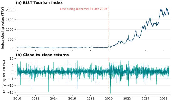
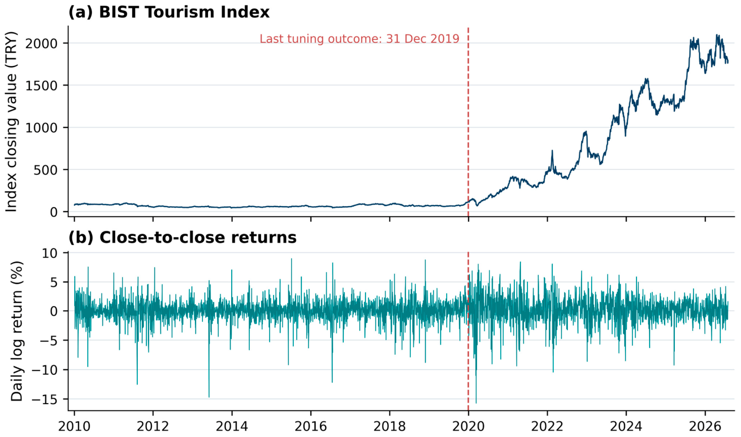
The cleaned index rose from 77.75 to 1790.60 over the full observation period. Upward outcomes accounted for 52.34% of all model-ready origins and 55.05% of the primary evaluation set. The corresponding intraday upward share was 50.97%. Figure 1 illustrates the level series and the final pre-2020 tuning-outcome boundary. The descriptive rise in the price index does not determine the profitability of strategies that hold only intraday.
Figure 1.
BIST Tourism Index closing values and daily log returns. The vertical line marks 31 December 2019, the last permitted tuning outcome date.
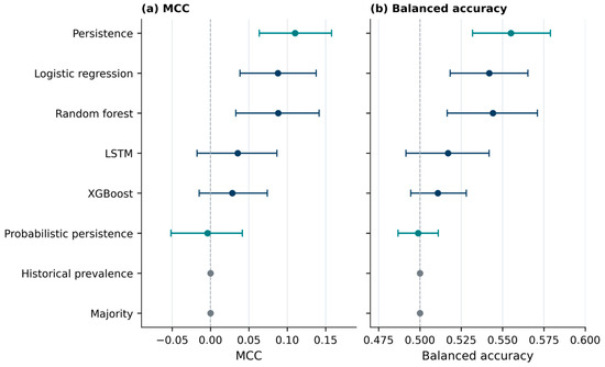
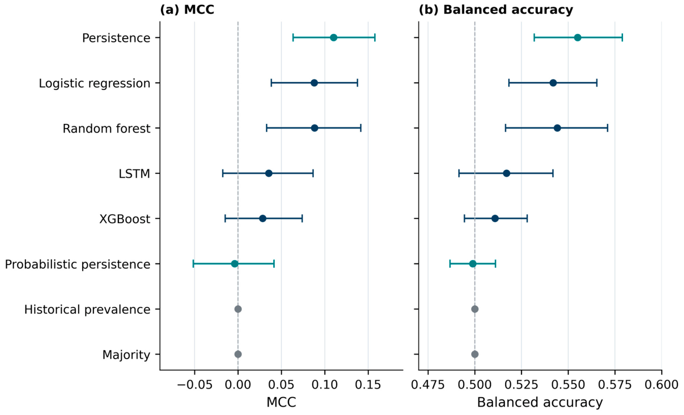
Directional persistence achieved the largest primary MCC (0.110). Random forest and logistic regression each achieved approximately 0.088, followed by LSTM (0.035) and XGBoost (0.028). Table 2 and Figure 2 show individual uncertainty. Historical prevalence and probabilistic persistence supplied probability benchmarks. Hard majority and persistence forecasts supplied directional comparators, whose 0/1 Brier scores are not calibrated probability estimates. Historical prevalence assumed 27 quarterly probability values. Its pooled ROC-AUC was 0.469, while its within-quarter ROC-AUC was 0.500.
Table 2.
Primary close-to-close forecasting performance (n = 1644).
Figure 2.
Primary MCC and balanced accuracy with individual conditional 95% intervals. Comparative evidence comes from paired differences. Points denote estimates and bars show individual intervals. Navy identifies fitted models, teal identifies persistence benchmarks, and gray identifies the majority and historical-prevalence benchmarks. The vertical dashed lines mark the reference values of 0 for MCC in panel (a) and 0.50 for balanced accuracy in panel (b).
The following comparisons are conditional on the recorded forecast paths, selected configurations, and fitted models. Logistic regression and random forest exceeded majority on MCC and balanced accuracy after Holm adjustment. Neither established primary MCC superiority over directional persistence. None of the six fitted-model MCC comparisons survived correction. Table 3 reports persistence contrasts. Table S4 reports paired comparisons for MCC, balanced accuracy, accuracy, and Brier score, and Table S5 reports block-length sensitivity.
Table 3.
Paired primary MCC differences from persistence.
XGBoost’s Brier score was 0.24610, compared with 0.24888 for historical prevalence and 0.24738 for probabilistic persistence. The model-minus-historical-prevalence difference was −0.00278, with a nominal 95% interval of −0.00481 to −0.00092 and Holm p = 0.060. The difference from probabilistic persistence was −0.00128, with an interval of −0.00311 to 0.00057 and Holm p = 1.000. Neither comparison established superiority in the primary eight-comparison Brier family. Against historical prevalence, adjusted p-values were 0.036 with five-observation blocks and 0.060 with twenty-observation blocks. No block length established superiority over probabilistic persistence (Table S13). The small pooled score improvement was therefore sensitive to benchmark and inferential specification.
Calendar-period classification results varied substantially. Logistic-regression MCC decreased from 0.128 in 2020–2021 to 0.085 in 2022–2023 and 0.061 in 2024–July 2026. Persistence increased from 0.081 to 0.111 and 0.131. XGBoost’s corresponding MCC values were −0.002, 0.122, and −0.021 (Table S3). Its Brier differences from probabilistic persistence were −0.00076, −0.00384, and 0.00031. None survived the within-period eight-comparison correction (Table S14). These are descriptive calendar comparisons. The suspension-record check used 1624 identical outcomes and excluded one changed outcome. In the controlled flat-label LSTM check, MCC was 0.055 for the same-environment reference and 0.064 after excluding flat training endpoints. The paired difference interval was −0.019 to 0.037 (Table S8).
Across three training seeds, random-forest MCC ranged from 0.088 to 0.099 and LSTM MCC from 0.035 to 0.070 (Table S9). Removing the designated return columns yielded a logistic-regression MCC of 0.097, removing volatility columns yielded 0.109, and removing technical/volume columns yielded 0.043. All paired difference intervals included zero (Table S10). These estimates describe sensitivity to column composition under the retained regularization setting. Pre-2020-selected thresholds removed the primary logistic-regression and random-forest advantages over majority (Table S11). Removing only the two provider-reported volume columns also removed those adjusted advantages. No fitted model established MCC superiority over persistence in that sensitivity (Table S12).
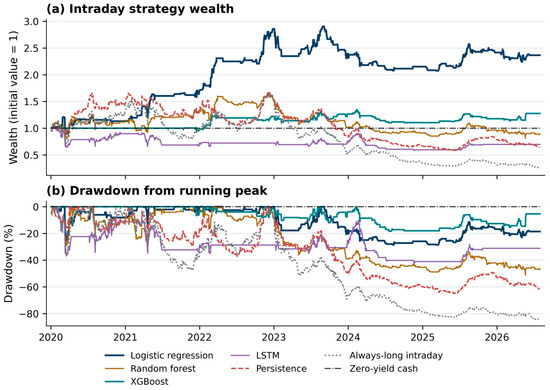
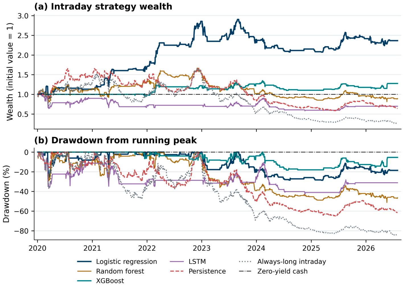
With intraday-specific selection, logistic regression achieved MCC 0.065, compared with 0.041 for intraday persistence. At ten basis points, CAGR was 14.11% (conditional 95% interval −2.85% to 34.49%), exposure was 25.06%, and maximum drawdown was −28.59%. The exploratory exposure-matched CAGR difference was 18.18 percentage points. Paired excess over the cash proxy was 16.35 percentage points, with an interval of −5.49 to 42.25 percentage points. Both the strategy-return and cash-excess intervals included zero. Table 4 and Table 5 and Figure 3 report pooled and period outcomes. Cumulative strategy returns under the zero-yield-cash assumption were 68.97%, 41.71%, and −1.20% across the three periods. Tables S6, S7, S15 and S16 provide transaction-cost, cash, and annual detail, including transferred-setting yearly returns. Table S18 compares configurations in the same environment.
Table 4.
Aligned intraday strategies at a 10-basis-point round-trip cost.
Table 5.
Logistic-regression returns with intraday-specific selection across calendar periods.
Figure 3.
Wealth and drawdown for the intraday-specific configurations at a ten-basis-point cost, including intraday persistence and the same-session always-long benchmark. Initial wealth is one and uninvested cash earns zero. Drawdowns are measured from the running wealth peak.
4. Discussion
The primary results, conditional on the recorded forecasts and fitted models, show why benchmark choice matters for sectoral forecasting. Logistic regression and random forest improved on the majority rule, while directional persistence attained the largest MCC point estimate. Paired comparisons accounting for temporal dependence and multiplicity did not establish fitted-model superiority over persistence. The logistic-regression-minus-persistence interval, approximately −0.078 to 0.035, permits differences in either direction. Accordingly, non-rejection does not establish equivalence, and the similar logistic-regression and random-forest point estimates do not establish a ranking.
Probability comparisons conditional on the recorded forecasts add a complementary assessment of predictive information. XGBoost achieved lower pooled Brier loss than both probability benchmarks, although neither primary adjusted comparison established superiority. Its difference from probabilistic persistence changed sign in the final calendar period. The small improvement over historical prevalence therefore needs to be interpreted alongside simple directional dependence and temporal variation. Brier scores measure probability loss. Calibration diagnostics and decision-specific evaluation would be needed to assess calibration quality and practical use.
These findings concern next-session forecasting for a single sector index. Large cross-sectional applications of deep and ensemble learning address different samples and estimation settings (Fischer & Krauss, 2018; Gu et al., 2020; Krauss et al., 2017). Here, approximately 4100 observations support a controlled comparison of four fitted models and explicit forecasting rules. Fixed pre-pandemic hyperparameters, sequence length, and stopping rules define the evaluated specifications. The findings can therefore inform comparable sectoral applications, with broader algorithm comparisons requiring evidence from additional settings.
The empirical contribution is to connect benchmark strength, information timing, and economic target alignment in an assessment of XTRZM. This complements the index-level forecasting evidence of Gülay et al. (2023) with direct comparisons of next-session direction and probability information. The first-order transition benchmark evaluates information beyond simple directional dependence. The independently selected intraday task then examines the economic objective over its actual holding period. Calendar-period and specification checks show how these comparisons vary within the sample. The distributed forecasts and return paths make the resulting evidence available for direct numerical verification. These elements offer a transparent empirical reference for tourism-finance forecasting and a basis for comparable work in other sectors.
Variation across the pandemic and recovery motivates attention to changing predictability (Liu et al., 2023; Lo, 2004; McLean & Pontiff, 2016; Sahiner et al., 2026). The calendar comparisons document that variation without identifying its causes or estimating distinct market regimes. Feature-group comparisons similarly evaluate sensitivity to the designated column sets. The exact reconstruction of the current return from retained technical predictors means that removing return-group columns preserves some return information. The paired intervals include zero, so these comparisons do not establish an advantage for the full feature set or the unique contribution of a group.
The intraday analysis shows the value of aligning configuration selection, forecast outcome, and holding period. Selection used pre-2020 intraday labels and was followed by quarterly fitting. The same-environment transferred-setting comparison assessed the effect of this configuration choice within the evaluation sample. Positive pooled return estimates accompanied material drawdown, calendar variation, and uncertain excess over the interest-bearing cash proxy. Exposure matching provides an additional reference for the strategy’s time in the market. Assessing an implementable strategy would also require a tradable instrument and its relevant execution costs (Novy-Marx & Velikov, 2016; Timmermann & Granger, 2004).
Limitations and Future Research
The scope of the findings is one price index, its provider-reported activity measure, and the documented retrospective design. The bootstrap compares recorded forecast paths while holding configuration selection and model fitting fixed. It therefore excludes uncertainty from repeating the entire estimation procedure. Seed replications and controlled refits assess selected sources of variability within that scope. Economic results describe hypothetical index-based strategies under stated cost and cash assumptions. Output verification is supported by the distributed files. Repeating the complete data-dependent pipeline additionally requires an authorized source export and the documented computational environment.
Future research could extend the comparison to additional tourism indices or constituent-stock panels and incorporate tourism-demand predictors. A new evaluation period would allow the prospective specification of probability calibration and decision thresholds. Resampling the full selection and fitting procedure would assess estimation uncertainty beyond the recorded forecast paths. Economic validation could use an actual investment instrument, an attainable cash yield, and its implementation costs.
5. Conclusions
This study provides sector-specific evidence on the incremental forecasting value of machine learning for the BIST Tourism Index. It evaluates directional and probability forecasts against explicit simple rules and assesses an intraday objective with independently selected configurations. Outcome-date controls link model selection and quarterly fitting to information available at each forecast origin. Paired comparisons and sensitivity analyses place the observed performance differences within a common evaluation framework.
At the primary 0.50 threshold and conditional on the recorded forecast paths, logistic regression and random forest exceeded the majority forecast. Directional persistence nevertheless achieved the highest MCC, and no fitted model established MCC superiority over it. The majority-rule advantages were sensitive to threshold choice and the removal of the volume columns. XGBoost’s small Brier reductions did not establish superiority over either probability benchmark in the primary adjusted comparisons. Intraday economic outcomes varied across time, with uncertain excess over the interest-bearing cash proxy. The evidence supports a benchmark-dependent assessment of predictive value and does not establish model equivalence or a reliable investment advantage.
The contribution lies in showing how directional dependence, probability loss, and a holding-period-aligned economic objective jointly shape the evaluation of forecasting gains in tourism finance. Full-precision forecasts, daily return paths, and the supplied verification command support direct checking of the reported results. The documented input requirements and estimation workflow also provide a clear route for extending the analysis with authorized data.
Supplementary Materials
The following supporting information can be downloaded at: https://www.mdpi.com/article/10.3390/ijfs14110324/s1. The supplementary ZIP archive contains Supplementary_Materials.docx with Tables S1–S18, the Analysis_Code folder, and publication figures in vector PDF/SVG and 600-dpi PNG/TIFF formats. The code folder provides forecasts, daily returns, evaluation tables, transition audits, configurations, tests, and computational records. Its verification guide maps the published tables to the distributed files. README.md gives separate instructions for output verification and full data-dependent reproduction. Table S1. Feature definitions; Table S2. Outcome-date-controlled model selection; Table S3. Primary MCC by calendar subperiod; Table S4. Paired comparisons for both forecast targets; Table S5. Primary MCC sensitivity to block length; Table S6. Holding-period and transaction-cost sensitivity; Table S7. Sensitivity to interest-bearing cash; Table S8. Data treatment on identical realized outcomes; Table S9. Training-seed sensitivity; Table S10. Logistic-regression feature-group ablation; Table S11. Pre-2020 threshold sensitivity; Table S12. Sensitivity to excluding the two volume predictors; Table S13. Brier comparisons against both probability benchmarks; Table S14. Brier differences across calendar periods; Table S15. Intraday economic outcomes by calendar period; Table S16. Logistic-regression intraday outcomes by outcome year; Table S17. Intraday-specific configuration selection; Table S18. Same-environment intraday configuration comparison.
Author Contributions
Conceptualization, İ.S.; methodology, İ.S.; software, H.K.; validation, İ.S., S.Ö.S., H.K. and N.G.; formal analysis, H.K.; investigation, İ.S. and S.Ö.S.; resources, S.Ö.S. and N.G.; data curation, H.K. and N.G.; writing—original draft, İ.S.; writing—review and editing, S.Ö.S. and N.G.; visualization, H.K.; supervision, İ.S.; project administration, İ.S.; funding acquisition, not applicable. All authors have read and agreed to the published version of the manuscript.
Funding
This research received no external funding.
Institutional Review Board Statement
Not applicable.
Informed Consent Statement
Not applicable.
Data Availability Statement
Date-aligned forecasts and labels, daily strategy returns, summary tables, analysis code, configurations, and computational records are distributed with the Supplementary Materials. The command python verify_results.py checks the analytical outputs without commercial source prices or model fitting. Source OHLCV observations were obtained from Investing.com and are excluded because redistribution permission has not been established. Full data-dependent reproduction requires an authorized export matching the documented schema and source fingerprint. Analysis_Code/README.md and VERIFICATION_GUIDE.md explain the two routes and their scope.
Acknowledgments
During the preparation of this study, the authors used ChatGPT (OpenAI, model GPT-6 Sol) and Codex (OpenAI, model GPT-6 Sol) to assist with developing the analysis code, preparing tables and figures, checking reference records, and language editing. The authors reviewed and edited the resulting code, outputs, and manuscript text and accept full responsibility for the content of this publication.
Conflicts of Interest
The authors declare no conflicts of interest.
References
- Ballings, M., Van den Poel, D., Hespeels, N., & Gryp, R. (2015). Evaluating multiple classifiers for stock price direction prediction. Expert Systems with Applications, 42(20), 7046–7056. [Google Scholar] [CrossRef] [Scilit]
- Bergmeir, C., & Benítez, J. M. (2012). On the use of cross-validation for time series predictor evaluation. Information Sciences, 191, 192–213. [Google Scholar] [CrossRef] [Scilit]
- Bergstra, J., & Bengio, Y. (2012). Random search for hyper-parameter optimization. Journal of Machine Learning Research, 13(10), 281–305. [Google Scholar]
- Bollinger, J. (2001). Bollinger on bollinger bands. McGraw-Hill. [Google Scholar]
- Borsa İstanbul. (n.d.). BIST tourism (XTRZM). Available online: https://borsaistanbul.com/en/index/xtrzm (accessed on 28 October 2026).
- Borsa İstanbul. (2023, February 8). Temporary suspension of trading in the equity market and single stock and index futures and options contracts in derivatives market for 5 business days and cancellation of trades on 08/02/2023. Public Disclosure Platform. Available online: https://www.kap.org.tr/en/Bildirim/1111497 (accessed on 2 October 2026).
- Borsa İstanbul. (2026). BIST piyasa değeri ağırlıklı pay endeksleri kural seti [BIST market-capitalization-weighted stock indices ground rules] (February 2026 version). Available online: https://www.borsaistanbul.com/files/bist-pd-agirlikli-pay-endeksleri-ks-tr-202601-temiz.pdf (accessed on 2 October 2026).
- Breiman, L. (2001). Random forests. Machine Learning, 45(1), 5–32. [Google Scholar] [CrossRef] [Scilit]
- Brier, G. W. (1950). Verification of forecasts expressed in terms of probability. Monthly Weather Review, 78(1), 1–3. [Google Scholar] [CrossRef] [Scilit]
- Central Bank of the Republic of Türkiye. (n.d.). 1 Hafta Repo [One-week repo auction interest rates]. Available online: https://www.tcmb.gov.tr/wps/wcm/connect/TR/TCMB%20TR/Main%20Menu/Temel%20Faaliyetler/Para%20Politikasi/Merkez%20Bankasi%20Faiz%20Oranlari/1%20Hafta%20Repo (accessed on 2 October 2026).
- Chen, T., & Guestrin, C. (2016). XGBoost: A scalable tree boosting system. In Proceedings of the 22nd ACM SIGKDD international conference on knowledge discovery and data mining (pp. 785–794). Association for Computing Machinery. [Google Scholar] [CrossRef] [Scilit]
- Chicco, D., & Jurman, G. (2020). The advantages of the Matthews correlation coefficient (MCC) over F1 score and accuracy in binary classification evaluation. BMC Genomics, 21(1), 6. [Google Scholar] [CrossRef] [Scilit] [PubMed]
- Fama, E. F. (1970). Efficient capital markets: A review of theory and empirical work. The Journal of Finance, 25(2), 383–417. [Google Scholar] [CrossRef] [Scilit]
- Fischer, T., & Krauss, C. (2018). Deep learning with long short-term memory networks for financial market predictions. European Journal of Operational Research, 270(2), 654–669. [Google Scholar] [CrossRef] [Scilit]
- Gössling, S., Scott, D., & Hall, C. M. (2021). Pandemics, tourism and global change: A rapid assessment of COVID-19. Journal of Sustainable Tourism, 29(1), 1–20. [Google Scholar] [CrossRef] [Scilit]
- Gu, S., Kelly, B., & Xiu, D. (2020). Empirical asset pricing via machine learning. The Review of Financial Studies, 33(5), 2223–2273. [Google Scholar] [CrossRef] [Scilit]
- Gülay, G., Armağan, İ. Ü., & Ergun, K. (2023). Interaction between tourism and Turkey’s capital markets: Analysis of Istanbul stock exchange tourism index. Journal of Gastronomy, Hospitality and Travel, 6(3), 1477–1490, [In Turkish]. [Google Scholar] [CrossRef] [Scilit]
- Helhel, Y., & Helhel, S. (2026). An assessment of economic and geopolitical risk sensitivity in the tourism sector: Evidence from firm-level performance and stock returns (2012–2025). Journal of Risk and Financial Management, 19(2), 102. [Google Scholar] [CrossRef] [Scilit]
- Hochreiter, S., & Schmidhuber, J. (1997). Long short-term memory. Neural Computation, 9(8), 1735–1780. [Google Scholar] [CrossRef] [Scilit] [PubMed]
- Holm, S. (1979). A simple sequentially rejective multiple test procedure. Scandinavian Journal of Statistics, 6(2), 65–70. [Google Scholar]
- Investing.com. (n.d.). BIST Turizm geçmiş verileri [BIST tourism historical data]. Available online: https://tr.investing.com/indices/ise-tourism-historical-data (accessed on 2 October 2026).
- Katircioglu, S., & Katircioglu, S. (2023). The effects of business and finance conditions on the tourism stock markets: An empirical investigation from Turkey. International Journal of Finance & Economics, 28(4), 4500–4511. [Google Scholar] [CrossRef] [Scilit]
- Kingma, D. P., & Ba, J. (2015, May 7–9). Adam: A method for stochastic optimization. 3rd International Conference on Learning Representations (ICLR), San Diego, CA, USA. [Google Scholar]
- Krauss, C., Do, X. A., & Huck, N. (2017). Deep neural networks, gradient-boosted trees, random forests: Statistical arbitrage on the S&P 500. European Journal of Operational Research, 259(2), 689–702. [Google Scholar] [CrossRef] [Scilit]
- Künsch, H. R. (1989). The jackknife and the bootstrap for general stationary observations. The Annals of Statistics, 17(3), 1217–1241. [Google Scholar] [CrossRef] [Scilit]
- Liu, Y., Cheng, X., Liao, S. S., & Yang, F. (2023). The impact of COVID-19 on the tourism and hospitality industry: Evidence from international stock markets. The North American Journal of Economics and Finance, 64, 101875. [Google Scholar] [CrossRef] [Scilit]
- Lo, A. W. (2004). The adaptive markets hypothesis. The Journal of Portfolio Management, 30(5), 15–29. [Google Scholar] [CrossRef] [Scilit]
- Matthews, B. W. (1975). Comparison of the predicted and observed secondary structure of T4 phage lysozyme. Biochimica et Biophysica Acta (BBA)—Protein Structure, 405(2), 442–451. [Google Scholar] [CrossRef] [Scilit] [PubMed]
- McLean, R. D., & Pontiff, J. (2016). Does academic research destroy stock return predictability? The Journal of Finance, 71(1), 5–32. [Google Scholar] [CrossRef] [Scilit]
- McNemar, Q. (1947). Note on the sampling error of the difference between correlated proportions or percentages. Psychometrika, 12(2), 153–157. [Google Scholar] [CrossRef] [Scilit] [PubMed]
- Novy-Marx, R., & Velikov, M. (2016). A taxonomy of anomalies and their trading costs. The Review of Financial Studies, 29(1), 104–147. [Google Scholar] [CrossRef] [Scilit]
- Paszke, A., Gross, S., Massa, F., Lerer, A., Bradbury, J., Chanan, G., Killeen, T., Lin, Z., Gimelshein, N., Antiga, L., Desmaison, A., Köpf, A., Yang, E., DeVito, Z., Raison, M., Tejani, A., Chilamkurthy, S., Steiner, B., Fang, L., … Chintala, S. (2019). PyTorch: An imperative style, high-performance deep learning library. In Advances in neural information processing systems 32. Curran Associates. [Google Scholar] [CrossRef] [Scilit]
- Patel, J., Shah, S., Thakkar, P., & Kotecha, K. (2015). Predicting stock and stock price index movement using trend deterministic data preparation and machine learning techniques. Expert Systems with Applications, 42(1), 259–268. [Google Scholar] [CrossRef] [Scilit]
- Pedregosa, F., Varoquaux, G., Gramfort, A., Michel, V., Thirion, B., Grisel, O., Blondel, M., Prettenhofer, P., Weiss, R., Dubourg, V., Vanderplas, J., Passos, A., Cournapeau, D., Brucher, M., Perrot, M., & Duchesnay, É. (2011). Scikit-learn: Machine learning in Python. Journal of Machine Learning Research, 12(85), 2825–2830. [Google Scholar]
- Pesaran, M. H., & Timmermann, A. (1992). A simple nonparametric test of predictive performance. Journal of Business & Economic Statistics, 10(4), 461–465. [Google Scholar] [CrossRef] [Scilit]
- Politis, D. N., & Romano, J. P. (1994). The stationary bootstrap. Journal of the American Statistical Association, 89(428), 1303–1313. [Google Scholar] [CrossRef]
- Sahiner, M., Khasawneh, M., & Korkusuz, B. (2026). From pandemic turbulence to recovery: A dynamic assessment of return and volatility spillovers in tourism finance. Financial Innovation, 12, 80. [Google Scholar] [CrossRef] [Scilit]
- Timmermann, A., & Granger, C. W. J. (2004). Efficient market hypothesis and forecasting. International Journal of Forecasting, 20(1), 15–27. [Google Scholar] [CrossRef] [Scilit]
- West, K. D. (1996). Asymptotic inference about predictive ability. Econometrica, 64(5), 1067–1084. [Google Scholar] [CrossRef] [Scilit]
- Wilder, J. W. (1978). New concepts in technical trading systems. Trend Research. [Google Scholar]
- Wu, W., Lee, C.-C., Xing, W., & Ho, S.-J. (2021). The impact of the COVID-19 outbreak on Chinese-listed tourism stocks. Financial Innovation, 7(1), 22. [Google Scholar] [CrossRef] [Scilit] [PubMed]

Disclaimer/Publisher’s Note: The statements, opinions and data contained in all publications are solely those of the individual author(s) and contributor(s) and not of MDPI and/or the editor(s). MDPI and/or the editor(s) disclaim responsibility for any injury to people or property resulting from any ideas, methods, instructions or products referred to in the content. |
© 2026 by the authors. Licensee MDPI, Basel, Switzerland. This article is an open access article distributed under the terms and conditions of the Creative Commons Attribution (CC BY) license.