A Five-State Markov Reliability Model for GEO Satellites with Sequential Degradation, Sudden Critical Transitions, and Functional Restoration

Abstract

Long-term GEO satellite operation requires reliability models that distinguish full mission capability from degraded but still functional states and from critical functional loss. This study develops a five-state Markov reliability model in which states S0–S4 represent successive levels of mission capability. The model integrates sequential degradation, a direct S0 → S4 transition representing sudden critical events, and functional restoration associated with redundancy, FDIR, reconfiguration, and software-supported recovery. Four computational variants were analysed over a segmented 15-year mission horizon to separate the influence of these mechanisms. The transition intensities were specified for a reference scenario rather than estimated for a specific GEO mission. Full and retained mission capability were evaluated using R_full = P₀ and R_partial = 1 − P₄. For the complete model, these measures reached 0.6926 and 0.9633 after 15 years, respectively. Calculations performed in MATLAB 2025 using the matrix exponential method were independently verified by numerical integration, with agreement within approximately 10⁻¹⁴. The framework provides a reproducible basis for analysing long-term GEO satellite functional reliability under different degradation and restoration scenarios.

1. Introduction

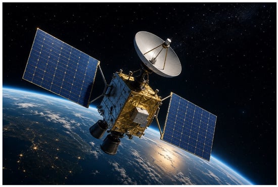
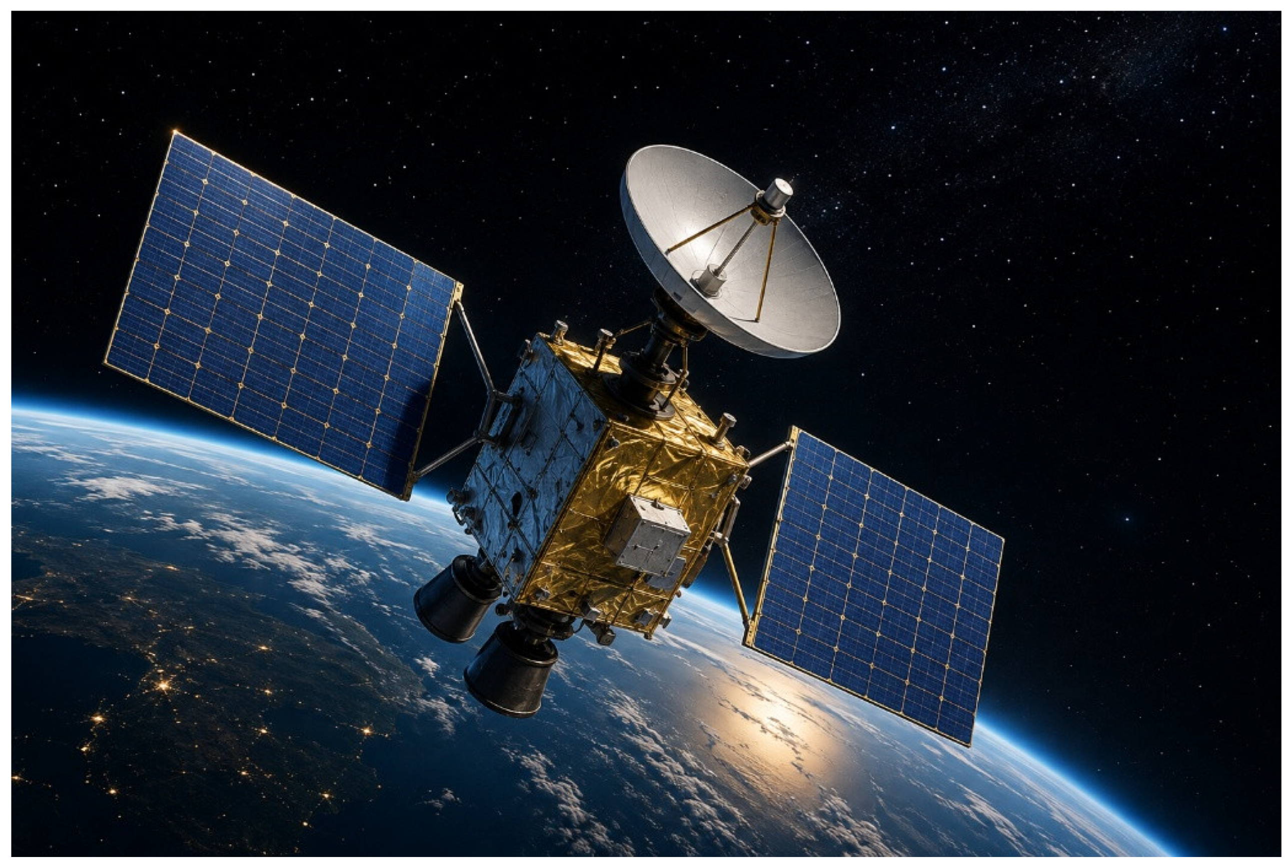
Geostationary satellites are long-life, high-value technical systems that provide continuous telecommunications, meteorological services, navigation support, Earth observation, and other mission services from an orbital altitude of approximately 35,786 km above the equator. Their operational lifetime frequently exceeds 15 years, during which the spacecraft must maintain critical mission functions despite progressive component aging, radiation exposure, thermal cycling, micrometeoroid and orbital-debris hazards, and the absence of conventional physical servicing. These conditions make reliability, redundancy, fault management, and functional recovery fundamental elements of GEO satellite design and operation [1,2,3,4]. An illustrative representation of a geostationary satellite is shown in Figure 1.

Figure 1. Illustrative representation of a geostationary satellite (GEO).

A GEO satellite consists of mutually dependent subsystems, including electrical power, communications, attitude and orbit control, propulsion, thermal control, on-board computing and fault management, and the structural platform. The loss or degradation of one subsystem does not necessarily result in immediate mission termination because spacecraft architectures commonly incorporate redundancy, alternative operational modes, and autonomous or ground-supported recovery mechanisms. Statistical studies of satellite populations have demonstrated that failure behaviour differs considerably between spacecraft architectures and individual subsystems and that the severity of observed anomalies cannot always be represented adequately by a simple distinction between operational and failed spacecraft states [1,2,3,4,5,6].

Correlated disturbances affecting power, thermal control, ADCS, or communication subsystems may accelerate the redistribution of probability from the fully functional state toward degraded or critical states; their explicit quantitative representation would, however, require a joint subsystem-state model with additional dependence parameters beyond the aggregated five-state formulation considered here.

This problem has motivated the use of multi-state reliability approaches in spacecraft engineering. In contrast to two-state representations, multi-state models allow the system to occupy several levels of operational capability and therefore preserve information about partial degradation before complete loss of functionality [2,3,7]. Such an approach is particularly relevant to satellite systems because degradation may develop gradually. Solar-array efficiency decreases with mission duration, battery capacity deteriorates, sensors and reaction wheels undergo aging, propulsion resources are progressively depleted, and electronic equipment remains exposed to cumulative radiation effects [8,9,10,11]. The spacecraft may therefore continue to perform its mission despite a measurable deterioration in technical or functional condition.

Gradual degradation is not, however, the only mechanism affecting satellite reliability. Spacecraft may also experience sudden events that produce a substantial loss of capability without passing through a complete sequence of intermediate degradation conditions. Examples include single-event effects in electronic systems, abrupt power-system anomalies, control-system malfunctions, propulsion failures, and damage associated with the space environment [4,9,10,12]. Reliability models intended for long-duration spacecraft operation should consequently distinguish progressive degradation from low-probability but potentially severe transitions capable of moving the system directly toward a critical functional condition. Multi-state models incorporating random shocks or non-sequential transitions provide a mathematical basis for representing this type of behaviour [13,14,15].

A further characteristic of spacecraft operation is that an anomaly does not necessarily result in an irreversible loss of capability. Fault detection, isolation, and recovery mechanisms may restore essential functions through switching to redundant units, system reconfiguration, software restart, safe-mode recovery, load redistribution, or the activation of alternative functional paths [16,17].

Previous studies have provided extensive knowledge on satellite reliability statistics, subsystem failures, multi-state system modelling, phased-mission reliability, and FDIR strategies [18,19]. However, these research directions are often considered separately. Statistical reliability studies focus primarily on observed anomalies and failures; multi-state models describe different technical or performance levels, while FDIR studies concentrate on detecting and recovering from faults. Less attention has been given to a unified functional representation in which progressive degradation, sudden critical loss, and restoration of mission capability are explicitly separated within the same state-transition structure. This distinction is particularly important because the loss of full functionality is not equivalent to the loss of the ability to continue the mission.

For this reason, the present study adopts a five-state functional classification S0–S4, following the concept of multi-valued technical-condition classification previously developed for complex technical systems [20] and adapting it to GEO satellite operation.

The proposed framework integrates three different transition mechanisms within one continuous-time Markov model. Sequential transitions S0 → S1 → S2 → S3 → S4 represent progressive degradation. A direct S0 → S4 transition represents sudden events capable of causing critical loss without observable progression through the intermediate states. Restoration transitions from S1–S4 to S0 represent the recovery of functional capability when such recovery is technically possible. In the case of an irreversible mission-ending event, the restoration intensity from S4 may be set to zero and S4 treated as an absorbing state.

The main research objective is to determine whether the simultaneous representation of these mechanisms provides a useful basis for distinguishing their respective effects on the long-term functional condition of a GEO satellite. To achieve this objective, four computational variants are considered. They separately represent sequential degradation, sequential degradation with functional restoration, sequential degradation with a direct critical transition, and the complete model incorporating all three mechanisms. This experimental structure enables the effects of restoration and sudden critical transitions to be identified independently rather than being combined within a single reliability trajectory.

Two complementary measures are used to interpret the calculated state probabilities. The first, R_full = P₀, represents the probability of maintaining full mission capability. The second, R_partial = 1 − P₄, represents the probability that critical mission capability is retained at time t. Their simultaneous evaluation preserves the contribution of states S1–S3 and therefore distinguishes complete functionality from degraded but still operational mission states. Particular attention is also given to S3 because its position immediately preceding the sequential transition to S4 gives it potential diagnostic significance as a pre-critical warning condition. The study does not, however, assume that S3 constitutes a validated operational intervention threshold; such an interpretation would require mission-specific telemetry and a formally defined decision policy.

The numerical experiment covers a 15-year GEO mission horizon divided into three operational intervals, allowing the transition intensities to change with mission age. The adopted λ and μ values define a reference computational scenario reflecting increasing degradation and reduced restoration capability during later mission periods; they are not parameters estimated from a complete operational dataset for a specific spacecraft. The purpose of the study is therefore not to predict the reliability of an individual GEO satellite but to provide a reproducible framework for analysing how sequential degradation, sudden critical transitions, and functional restoration jointly influence long-term mission capability.

2. Characteristics of the GEO Satellite

A geostationary satellite operates at an altitude of approximately 35,786 km above the equator, with an orbital period synchronized with the Earth’s rotation. This orbital configuration enables continuous coverage of the same geographical region and is therefore particularly suitable for long-duration telecommunications and data-relay missions. GEO satellites are typically designed for operational lifetimes of approximately 15 years or longer, during which their functional capability depends on the continued operation of several strongly coupled spacecraft subsystems.

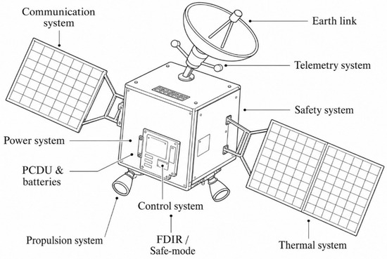
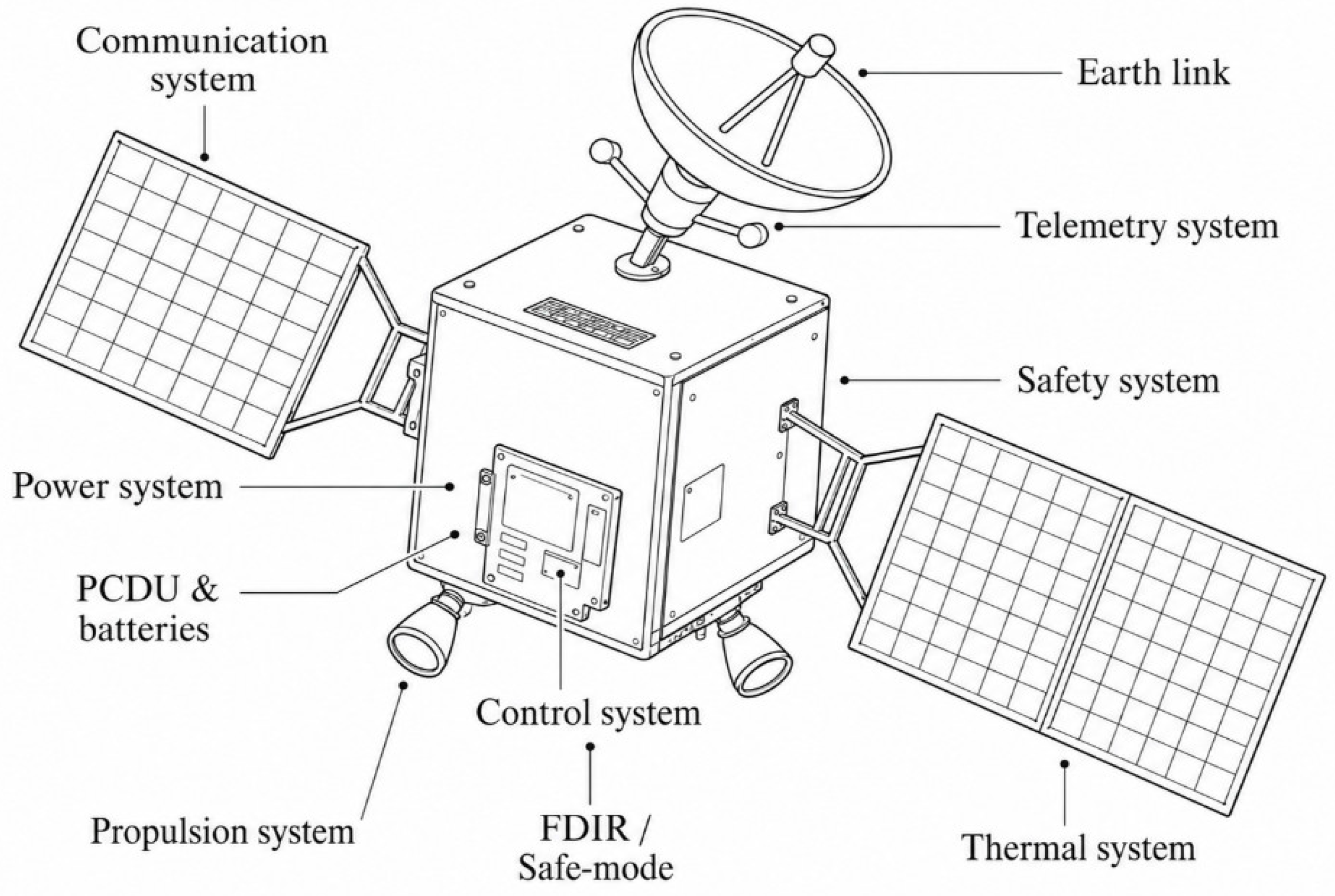
The GEO satellite considered in this study is represented by its principal functional subsystems responsible for maintaining mission capability. These include the structural framework, electrical power system, attitude and orbit control system, communication and telemetry systems, thermal control, onboard computer and fault detection, isolation and recovery functions, propulsion, and mission-related equipment. Their functional arrangement is illustrated in Figure 2.

Figure 2. Example architecture of a GEO satellite with the principal functional subsystems.

Long-duration GEO operation is associated with progressive degradation caused by thermal cycling, radiation exposure, aging of photovoltaic arrays and batteries, wear of attitude-control and propulsion components, and degradation of electronic equipment. In addition to gradual deterioration, the spacecraft may experience sudden events such as radiation-induced electronic anomalies, critical power disturbances, loss of communication capability, attitude-control anomalies, or damage associated with the orbital environment. The resulting effects may propagate between functionally coupled subsystems and lead to different levels of degradation in mission capability.

Physical repair of a GEO satellite is generally unavailable during nominal mission operation. Consequently, recovery of functionality is primarily achieved through onboard and ground-supported mechanisms such as redundancy activation, system reconfiguration, safe-mode operation, software recovery, load redistribution, or switching to alternative functional paths. This distinction is essential because restoration in the reliability model represents recovery of functional capability rather than conventional physical repair.

The principal subsystem groups, representative degradation mechanisms, and corresponding functional restoration mechanisms are summarized in Table 1. The classification provides the engineering basis for associating observed or assumed subsystem degradation with the degradation and restoration transitions used in the five-state model.

Table 1. Main subsystems of a GEO satellite, dominant degradation mechanisms, and relation to degradation and functional restoration processes in the five-state reliability model.

Subsystem	Key Components	Dominant Degradation Mechanisms	Effect on Functional Capability	Degradation and Functional Restoration Processes
Structural Framework	CFRP/Al panels, Ti joints, honeycomb panels	Thermal cycling, micrometeoroid and orbital debris impact, material fatigue	Deformation, crack initiation, loss of mechanical and thermal stability	Structural degradation may be non-restorable; its functional effects may be mitigated through available system-level redundancy or operational reconfiguration
Power Supply	III–V PV panels, Li-ion batteries, PDU, DC–DC converters	PV cell degradation, battery aging and capacity fade, radiation-induced degradation, converter aging	Reduced power availability, voltage drop, load limitations, possible power interruptions	Performance degradation; reconfiguration, load shedding, and activation of redundant power paths
ADCS	Star and Sun sensors, IMU, reaction wheels, magnetorquers, RCS thrusters	Reaction-wheel wear, sensor degradation or failure, radiation effects, thruster degradation	Reduced pointing accuracy, degradation of attitude knowledge, loss of control authority	Switching to redundant sensors or actuators, desaturation using RCS, control reconfiguration
Communications and TT&C	S/L/X/Ka-band transceivers, low- and high-gain antennas	Single-event effects, component aging, frequency or phase drift, antenna degradation	Link degradation or loss, reduced data rate, increased BER	Frequency switching, redundant communication paths, transponder reconfiguration, power reallocation
Thermal Control	MLI, radiators, heaters, heat pipes	Thermal cycling, coating degradation, heater aging	Temperature drift, local hot or cold regions, increased thermal risk	Heater-control adjustment, operational thermal management, mode reconfiguration
On-board Computer and FDIR	Redundant OBCs, ECC memory, watchdogs, safe-mode logic	SEU/SEL radiation effects, software anomalies, memory and electronic component aging	Processor reset, data corruption, software interruption, transition to degraded operating modes	Processor restart, software recovery, rollback, reconfiguration, FDIR actions
Propulsion	Chemical or electric thrusters, fuel or xenon tanks, valves	Propellant depletion, valve wear or leakage, radiation effects on electronics	Reduced manoeuvring capability, limited orbit or attitude maintenance	Thrust-profile optimisation, switching to redundant thrusters, propellant-management strategies

Degradation mechanisms contribute to transitions toward lower functional states, with the corresponding transition intensities represented by λ₁–λ₅, whereas functional restoration mechanisms support transitions toward improved functional capability represented by μ₁–μ₄.

2.1. Functional Interpretation and Justification of the Five-State Model

The five-state model is adopted to represent the evolution of the mission capability of a geostationary satellite under gradual degradation, sudden critical disturbances, and functional-restoration actions. The states should therefore be interpreted as levels of functional capability rather than as direct measures of physical damage. This distinction is particularly important for GEO satellites, for which physical servicing is generally unavailable, while functional recovery may still be achieved through redundancy, system reconfiguration, safe-mode recovery, software actions, load redistribution, or activation of backup components.

Models with fewer states can represent general transitions between operational and failed conditions but may obscure intermediate degradation levels that are relevant to condition assessment and operational intervention. The five-state representation retains three intermediate stages between nominal operation and loss of critical mission capability, thereby allowing gradual deterioration to be distinguished from abrupt functional loss and enabling the pre-critical condition to be analysed explicitly.

State S0 represents full mission capability, in which the satellite or the considered subsystem performs all required functions within the specified operational limits. State S1 represents minor functional degradation, in which measurable deterioration is present but does not significantly restrict the execution of primary mission functions. State S2 represents moderate degradation associated with reduced performance, operational restrictions, or the need to modify operating conditions. State S3 represents a pre-critical functional condition in which substantial degradation has occurred and continued operation remains possible, although the probability of losing critical capability is increased. State S4 represents loss of critical mission capability, in which the satellite or subsystem cannot perform one or more functions required for normal mission execution. To provide a direct engineering interpretation of the proposed classification, Table 2 relates states S0–S4 to representative measurable spacecraft indicators and corresponding operational conditions.

Table 2. Functional interpretation of the five-state GEO satellite model and representative measurable indicators.

State	Functional Interpretation	Representative Measurable Indicators
S0	Full mission capability within specified operational limits	nominal power margin, pointing accuracy, communication performance, thermal conditions and redundancy availability
S1	Minor measurable degradation without restriction of primary mission functions	small deterioration of power margin, pointing accuracy, link quality or other monitored parameters
S2	Moderate degradation requiring operational adaptation or restrictions	reduced power margin or throughput, increased pointing error, reduced redundancy, thermal or operational limitations
S3	Pre-critical condition with substantial degradation and increased risk of loss of critical capability	monitored parameters approaching mission-specific operational limits, repeated FDIR actions or persistent degraded operating mode
S4	Loss of critical mission capability	mission-specific critical limits exceeded or inability to maintain one or more functions required for mission execution

Specific numerical thresholds separating S0–S4 are mission- and platform-dependent and should be defined using spacecraft telemetry, operational limits, and mission requirements of the analysed spacecraft.

In this framework, S4 does not necessarily correspond to irreversible physical destruction of the satellite. In recoverable cases, critical mission capability may be restored through system-level actions such as redundancy activation, reconfiguration, safe-mode recovery, software reset, or other compensatory procedures. Consequently, the transition S4 → S0 represents functional restoration rather than physical repair. For scenarios in which the loss of critical capability is irreversible, the restoration intensity μ₄ is set to zero, and S4 becomes an absorbing state.

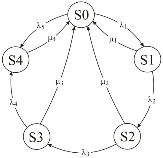
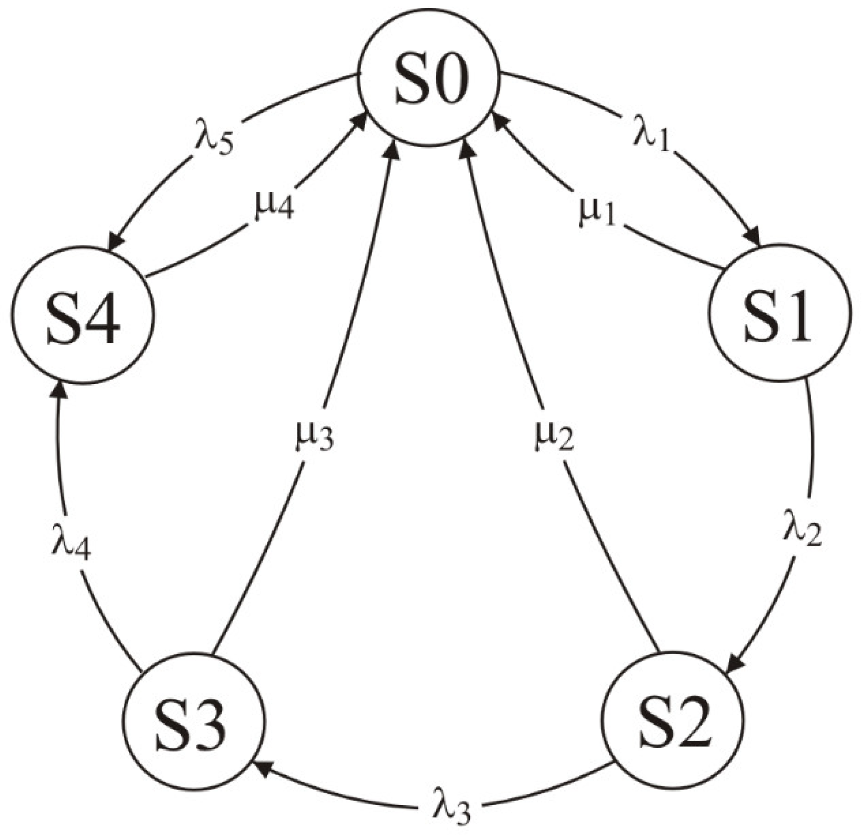
The transition structure adopted in the model is shown in Figure 3. Sequential degradation is represented by λ₁ for S0 → S1, λ₂ for S1 → S2, λ₃ for S2 → S3, and λ₄ for S3 → S4. In addition to this progressive degradation path, λ₅ represents a direct transition from S0 to S4 caused by a sudden critical event. This transition accounts for disturbances that may cause an immediate loss of critical mission capability without observable progression through the intermediate functional states.

Figure 3. Transition-Intensity Network of the Five-State GEO Satellite Model.

Restoration transitions μ₁, μ₂, μ₃, and μ₄ describe the return from S1, S2, S3, and S4, respectively, to the nominal functional state S0. They represent restoration of mission capability through actions available during GEO satellite operation, including reconfiguration, switching to redundant components, modification of operating modes, software recovery, or other compensatory actions performed autonomously or from the ground segment.

The resulting graph therefore represents three mechanisms of functional evolution. The first is gradual sequential degradation through S0 → S1 → S2 → S3 → S4, whereas the second is an abrupt critical transition S0 → S4. Restoration transitions provide an aggregated representation of the capability of the satellite or its subsystems to recover nominal functionality following degradation. The direct S_i → S0 transitions therefore represent successful restoration events that recover nominal mission capability rather than physical restoration of degraded hardware to its beginning-of-life condition. Skip transitions between intermediate degraded states and partial recoveries to another degraded state are physically possible, but their explicit representation would require additional transition intensities and an extended transition topology beyond the intentionally aggregated structure adopted in the present model. The numerical parameterization of λ and μ is treated separately from the structural definition of the model, with empirically supported values distinguished from reference or scenario-based assumptions.

2.2. Mathematical Model

A formal mathematical framework makes it possible to translate the intuitive transition graph into a well-defined system of equations that can be solved and numerically verified. This process begins with the construction of the Q matrix, which represents the complete transition structure of the five-state model. Based on this matrix, a system of differential equations is formulated to describe the evolution of the state probabilities over time. The same model can subsequently be analysed in the steady state using balance equations. Two equivalent algebraic forms are used for the steady-state solution, namely the stepwise form and the expanded independent form, while the integral representation is used to describe the transient evolution of the state probabilities.

For the transition network presented in Figure 3, the generator matrix Q is defined as:

$$Q=\left[\begin{array}{c}-({\lambda }_1+{\lambda }_5)\\ \begin{array}{c}{\mu }_1\\ \begin{array}{c}{\mu }_2\\ \begin{array}{c}{\mu }_3\\ {\mu }_4\end{array}\end{array}\end{array}\end{array}\begin{array}{c}{\lambda }_1\\ \begin{array}{c}-({\mu }_1+{\lambda }_2)\\ \begin{array}{c}0\\ \begin{array}{c}0\\ 0\end{array}\end{array}\end{array}\end{array}\begin{array}{c}0\\ \begin{array}{c}{\lambda }_2\\ \begin{array}{c}-({\mu }_2+{\lambda }_3)\\ \begin{array}{c}0\\ 0\end{array}\end{array}\end{array}\end{array}\begin{array}{c}0\\ \begin{array}{c}0\\ \begin{array}{c}{\lambda }_3\\ \begin{array}{c}-({\mu }_3+{\lambda }_4)\\ 0\end{array}\end{array}\end{array}\end{array}\begin{array}{c}{\lambda }_5\\ \begin{array}{c}0\\ \begin{array}{c}0\\ \begin{array}{c}{\lambda }_4\\ -{\mu }_4\end{array}\end{array}\end{array}\end{array}\right]$$

(1)

The off-diagonal elements of Q represent the transition intensities between individual states, while each diagonal element is equal to the negative sum of the intensities of all transitions leaving the corresponding state. Consequently, the sum of the elements in each row of Q is equal to zero.

The evolution of the state probabilities is described by the Kolmogorov forward equation. The state-probability vector and the normalization condition are defined as:

$$\dot{P}(t)=P(t)Q, P(t)=[P_0(t),P_1(t),P_2(t),P_3(t),P_4(t)], {\displaystyle \sum _{i=0}^4}{P}_i(t)=1$$

(2)

The model assumes that at the beginning of the analysed mission period the satellite is in state S0, which corresponds to P₀(0) = 1 and P₁(0) = P₂(0) = P₃(0) = P₄(0) = 0.

By expanding Equation (2), the system of differential equations describing the probability flows between states is obtained as:

$$\begin{array}{l}{{\dot{P}}_0=\mu }_1{P}_1+{\mu }_2{P}_2+{\mu }_3{P}_3+{\mu }_4{P}_4- ({\lambda }_1+{\lambda }_5)P_0\\ \begin{array}{l}{{\dot{P}}_1=\lambda }_1{P}_0- ({\mu }_1+{\lambda }_2)P_1\\ \begin{array}{l}{{\dot{P}}_2=\lambda }_2{P}_1- ({\mu }_2+{\lambda }_3)P_2\\ \begin{array}{l}{{\dot{P}}_3=\lambda }_3{P}_2- ({\mu }_3+{\lambda }_4)P_3\\ {{\dot{P}}_4=\lambda }_5{P}_0+{\lambda }_4{P}_3-{\mu }_4{P}_4\end{array}\end{array}\end{array}\end{array}$$

(3)

The first four equations describe the sequential degradation and restoration paths, whereas the last equation additionally includes the direct transition S0 → S4 represented by λ₅. This transition accounts for a sudden loss of critical mission capability without progression through the intermediate states.

The steady-state probabilities P₀–P₄ are obtained by setting all derivatives in Equation (3) equal to zero. The resulting balance equations are expressed as:

$$\left\{\begin{array}{l}{\mu }_1{P}_1+{\mu }_2{P}_2+{\mu }_3{P}_3+{\mu }_4{P}_4-({\lambda }_1+{\lambda }_5)P_0=0\\ \begin{array}{l}{\lambda }_1{P}_0-({\mu }_1+{\lambda }_2)P_1=0\\ \begin{array}{l}{\lambda }_2{P}_1-({\mu }_2+{\lambda }_3)P_2=0\\ \begin{array}{l}{\lambda }_3{P}_2-({\mu }_3+{\lambda }_4)P_3=0\\ {\lambda }_5{P}_0+{\lambda }_4{P}_3-{\mu }_4{P}_4=0\end{array}\end{array}\end{array}\end{array}\right.$$

(4)

The balance equations can first be solved using the stepwise form. The probability P₁ is expressed in terms of P₀ as:

$$P_1={\displaystyle \frac{{\lambda }_1}{{\mu }_1+{\lambda }_2}}{P}_0$$

(5)

The probability P₂ is then obtained as:

$$P_2={\displaystyle \frac{{\lambda }_2}{{\mu }_2+{\lambda }_3}}{P}_1= {\displaystyle \frac{{\lambda }_1{\lambda }_2}{{(\mu }_1+{\lambda }_2)({\mu }_2+{\lambda }_3)}}{P}_0$$

(6)

The probability P₃ is obtained as:

$$P_3={\displaystyle \frac{{\lambda }_3}{{\mu }_3+{\lambda }_4}}{P}_2={\displaystyle \frac{{\lambda }_1{\lambda }_2{\lambda }_3}{{(\mu }_1+{\lambda }_2)({\mu }_2+{\lambda }_3)({\mu }_3+{\lambda }_4)}}{P}_0$$

(7)

The probability P₄ accounts for both the direct transition S0 → S4 and the sequential transition S3 → S4, and is expressed as:

$$P_4={\displaystyle \frac{{\lambda }_5{P}_0+{\lambda }_4{P}_3}{{\mu }_4}}$$

(8)

The steady-state probabilities satisfy the normalization condition:

$$P_0+P_1+P_2+P_3+P_4=1$$

(9)

Substitution of Equations (5)–(8) into Equation (9) gives the probability of state S0 in the following form:

$$P_0={\displaystyle \frac{{(\mu }_1+{\lambda }_2)({\mu }_2+{\lambda }_3)({\mu }_3+{\lambda }_4){\mu }_4}{\begin{array}{c}{(\mu }_1+{\lambda }_2)({\mu }_2+{\lambda }_3)({\mu }_3+{\lambda }_4){\mu }_4+{\lambda }_1({\mu }_2+{\lambda }_3)({\mu }_3+{\lambda }_4){\mu }_4\\ \begin{array}{c}+{\lambda }_1{\lambda }_2({\mu }_3+{\lambda }_4){\mu }_4+{\lambda }_1{\lambda }_2{\lambda }_3{\mu }_4+{\lambda }_5{(\mu }_1+{\lambda }_2)({\mu }_2+{\lambda }_3)({\mu }_3+{\lambda }_4)\\ +{\lambda }_4{\lambda }_1{\lambda }_2{\lambda }_3\end{array}\end{array}}}$$

(10)

For direct computation, the same steady-state solution can be written in an expanded independent form. The common denominator M is defined as:

$$\begin{array}{c}{M=(\mu }_1+{\lambda }_2)({\mu }_2+{\lambda }_3)({\mu }_3+{\lambda }_4){\mu }_4+{\lambda }_1({\mu }_2+{\lambda }_3)({\mu }_3+{\lambda }_4){\mu }_4\\ \begin{array}{c}+{\lambda }_1{\lambda }_2({\mu }_3+{\lambda }_4){\mu }_4+{\lambda }_1{\lambda }_2{\lambda }_3{\mu }_4+{\lambda }_5{(\mu }_1+{\lambda }_2)({\mu }_2+{\lambda }_3)({\mu }_3+{\lambda }_4)\\ +{\lambda }_4{\lambda }_1{\lambda }_2{\lambda }_3\end{array}\end{array}$$

(11)

Using the common denominator M, the remaining state probabilities are determined directly as:

$$P_1={\displaystyle \frac{{\lambda }_1({\mu }_2+{\lambda }_3)({\mu }_3+{\lambda }_4){\mu }_4}{M}}$$

(12)

$$P_2={\displaystyle \frac{{\lambda }_1{\lambda }_2({\mu }_3+{\lambda }_4){\mu }_4}{M}}$$

(13)

$$P_3={\displaystyle \frac{{\lambda }_1{\lambda }_2{\lambda }_3{\mu }_4}{M}}$$

(14)

$$P_4={\displaystyle \frac{{\lambda }_5{(\mu }_1+{\lambda }_2)({\mu }_2+{\lambda }_3)({\mu }_3+{\lambda }_4)+{\lambda }_4{\lambda }_1{\lambda }_2{\lambda }_3}{M}}$$

(15)

Equations (5)–(15) describe the steady-state solution of the model for μ₄ > 0. This condition corresponds to the interpretation adopted in Section 2.1, in which state S4 represents a loss of critical mission capability that can, in selected cases, be restored functionally through reconfiguration, redundancy activation, safe-mode recovery, software actions, or other compensatory procedures. If μ₄ = 0, state S4 becomes absorbing and the steady-state expressions involving division by μ₄ are not applicable.

The transient behaviour of the model can additionally be expressed in integral form. Under the initial condition P₀(0) = 1 and P₁(0) = P₂(0) = P₃(0) = P₄(0) = 0, the probability P₁(t) is expressed as:

$$P_1(t)={\int }_0^t{\lambda }_1{P}_0(\tau )e^{-({\mu }_1+{\lambda }_2)(t-\tau )}d\tau$$

(16)

The probability P₂(t) is expressed as:

$$P_2(t)={\int }_0^t{\lambda }_2{P}_1(\tau )e^{-({\mu }_2+{\lambda }_3)(t-\tau )}d\tau$$

(17)

The probability P₃(t) is expressed as:

$$P_3(t)={\int }_0^t{\lambda }_3{P}_2(\tau )e^{-({\mu }_3+{\lambda }_4)(t-\tau )}d\tau$$

(18)

The probability P₄(t) includes inflow from both the sequential transition S3 → S4 and the direct transition S0 → S4, and is expressed as:

$$P_4(t)={\int }_0^t{[\lambda }_4{P}_3(\tau )+{\lambda }_5{P}_0(\tau )]e^{-{\mu }_4(t-\tau )}d\tau$$

(19)

The evolution of P₀(t) is determined by the corresponding differential balance equation:

$$P_0(t)={\mu }_1{P}_1(t)+{\mu }_2{P}_2(t)+{\mu }_3{P}_3(t)+{\mu }_4{P}_4(t)-({\lambda }_1+{\lambda }_5)P_0(t)$$

(20)

At each time instant, the probability normalization condition must remain satisfied:

$${\displaystyle \sum _{i=0}^4}{P}_i(t)=1$$

(21)

The integral representation in Equations (16)–(20) is equivalent to the differential formulation in Equation (3) under the adopted initial conditions. It provides a recursive description of the probability inflow to successive degradation states while explicitly accounting for the rate at which probability leaves each state. The steady-state and transient formulations therefore describe complementary aspects of the same five-state model. The steady-state equations characterize the long-term distribution for constant transition intensities and μ₄ > 0, whereas the transient equations describe the evolution of the GEO satellite functional state over a finite mission horizon.

2.3. Description of the Simulation Experiment

The analysis covered a 15-year mission horizon divided into three operational intervals of 0–5, 5–10, and 10–15 years. Within each interval, the transition intensities λ and μ were assumed to remain constant, while their values could change between consecutive intervals to represent the evolution of degradation and restoration conditions during the satellite lifetime. The probability vector obtained at the end of each interval was used as the initial condition for the subsequent interval.

The initial condition was defined as P₀(0) = 1 and P₁(0) = P₂(0) = P₃(0) = P₄(0) = 0. The time-dependent probabilities P₀(t)–P₄(t) were calculated over the complete mission horizon using the transition generator matrix Q. A computational step of 0.5 years was adopted, with detailed results evaluated after 5, 10, and 15 years of operation.

The computational procedure was implemented in MATLAB. The probability trajectories were determined using the matrix exponential formulation and independently verified by numerical integration of the corresponding system of ordinary differential equations. Numerical consistency was assessed by verifying the normalization condition $\sum P_i(t)=1$ and the non-negativity of all state probabilities throughout the analysed mission horizon.

The principal output quantities were the state probabilities P₀(t)–P₄(t), the full functional capability measure R_full = P₀, and the partial functional capability measure R_partial = 1 − P₄. The adopted parameter sets for λ and μ were assigned separately to the three mission intervals, enabling the influence of changing degradation and restoration conditions on the long-term functional state of the GEO satellite to be assessed.

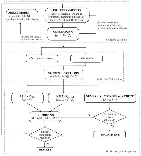
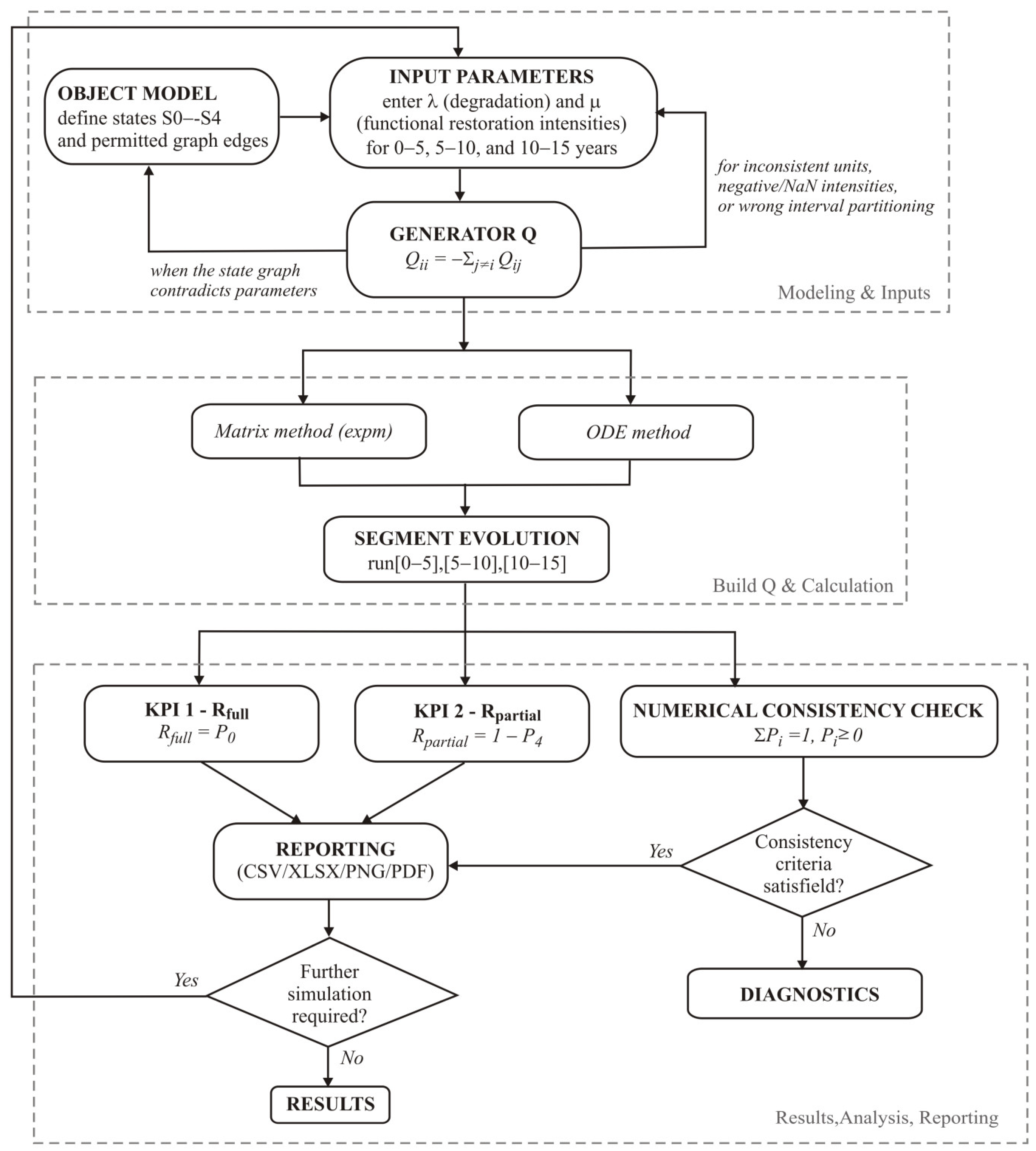
The computational procedure is presented in Figure 4.

Figure 4. Segmented-Time Reliability Computation Algorithm for the Five-State Model.

3. Numerical Results

The numerical analysis was performed for the five-state GEO satellite model over a 15-year mission horizon. The mission period was divided into three intervals of 0–5, 5–10, and 10–15 years, within which the transition intensities were assumed to remain constant. The probability vector obtained at the end of each interval was used as the initial condition for the subsequent interval. The three five-year intervals represent parameterization periods of the reference scenario rather than numerical integration steps. Because the solution within each interval is obtained using the matrix exponential, subdividing an interval into shorter subintervals while retaining the same transition matrix Q does not change the resulting state probabilities. A one- or two-year segmentation would therefore affect the results only if additional time-dependent transition intensities were introduced. The initial condition was defined as P₀(0) = 1 and P₁(0) = P₂(0) = P₃(0) = P₄(0) = 0.

The engineering basis for the segment-dependent transition-intensity assumptions is summarized in Table 3. The listed environmental, operational, and aging-related mechanisms provide the basis for the assumed changes in degradation and functional restoration conditions over the satellite mission. The adopted transition intensities therefore represent a reference computational scenario informed by published satellite reliability, subsystem-failure, anomaly, and space-environment studies [4,7,8,9,10], rather than parameters estimated for a specific GEO platform. The parameter changes at the 5- and 10-year mission boundaries are therefore interpreted as a piecewise-constant approximation of continuous physical degradation and recovery trends rather than as instantaneous changes in the spacecraft condition.

Table 3. Engineering basis for the segment-dependent transition-intensity assumptions.

Degradation or Recovery Factor	Main Affected Subsystem(s)	Mission-Time Dependence	Relation to the Five-State Model
Radiation and single-event effects	COMM, OBC, ADCS	Cumulative and episodic over the mission lifetime	Increase in degradation-transition intensities; severe events may contribute to λ5
Photovoltaic-array and battery aging	POW	Increasing with mission duration	Progressive increase in λ1–λ3
Reaction-wheel and sensor degradation	ADCS	Increasing, particularly in later mission intervals	Increase in sequential degradation intensities λ1–λ4
Propellant depletion and valve degradation	PROP	Predominantly cumulative	Increasing probability of transitions toward S2–S4
Thermal cycling and material degradation	THM, STR, COMM	Cumulative throughout the mission	Progressive increase in degradation intensities
Micrometeoroid and orbital-debris exposure	STR	Low-probability episodic events	Contribution primarily to sudden critical transition λ5
Electronic and software aging	OBC	Increasing with mission time, with possible abrupt anomalies	Sequential degradation and occasional contribution to λ5
Availability of redundancy and functional recovery resources	COMM, POW, ADCS, OBC, THM	Progressive reduction in available redundancy, backup resources, and viable FDIR/reconfiguration options with mission duration	Decreasing restoration intensities μ1–μ4; in the reference scenario, μ1–μ3 decrease by 50% between the first and final mission intervals, while μ4 decreases from 0.01 to 0.005 year−1

The transition intensities λ₁–λ₅ and μ₁–μ₄ are treated in the present study as effective system-level parameters of the functional-state model and are not obtained by mathematical aggregation of subsystem-specific failure or recovery rates.

The numerical values of λ₁–λ₅ and μ₁–μ₄ adopted in the reference scenario are presented in Table 4. The parameters remain constant within each mission interval and change at the boundaries of the 0–5, 5–10, and 10–15 year segments.

Table 4. Reference transition intensities for the GEO five-state model (units: 1/year).

Parameter	Transition	0–5 Years	5–10 Years	10–15 Years
λ1	S0 → S1	0.05	0.08	0.12
λ2	S1 → S2	0.03	0.05	0.08
λ3	S2 → S3	0.02	0.04	0.07
λ4	S3 → S4	0.005	0.01	0.05
λ5	S0 → S4	0.002	0.003	0.004
μ1	S1 → S0	0.6	0.45	0.3
μ2	S2 → S0	0.4	0.3	0.2
μ3	S3 → S0	0.2	0.15	0.1
μ4	S4 → S0	0.01	0.01	0.005

Four computational variants were defined to separate the effects of sequential degradation, functional restoration, and the direct transition S0 → S4. Their configuration is presented in Table 5. Variant A includes sequential degradation only, Variant B additionally includes functional restoration, Variant C additionally accounts for the direct critical transition, and Variant D represents the complete model.

Table 5. Computational variants used in the GEO reliability analysis.

Variant	λ1–λ4	λ5	μ1–μ4	Model Interpretation
A—DEG	Active	0	0	Sequential degradation only
B—DEG + REST	Active	0	Active	Sequential degradation with functional restoration
C—DEG + JUMP	Active	Active	0	Sequential degradation with sudden S0 → S4 transition
D—FULL	Active	Active	Active	Complete degradation, sudden-transition, and functional-restoration model

All calculations were performed in MATLAB 2025. State probabilities were determined using the matrix exponential solution of the continuous-time Markov model and independently verified by numerical integration of the corresponding ordinary differential equations. The maximum deviation from the normalization condition $\sum P_i(t)=1$ was below 9 × 10⁻¹⁶, while the maximum difference between the matrix and ODE solutions remained below 1.6 × 10⁻¹⁴. All state probabilities remained non-negative throughout the 15-year mission horizon.

Two system-level measures were evaluated:

$$R_{full}=P_0$$

(22)

$$R_{partial}={1-P}_4$$

(23)

For variants including functional restoration, R_full and R_partial are interpreted as instantaneous functional-capability measures rather than classical first-passage reliability functions. In particular, R_partial = 1 − P4 describes the probability that the system is outside S4 at time t and does not exclude a previous entry into S4 followed by functional restoration.

Table 6 presents R_full and R_partial for all four computational variants at 5, 10, and 15 years. These time points correspond to the boundaries of the adopted mission intervals.

Table 6. Functional capability measures of the GEO model for the four computational variants.

Variant	Time [Years]	Rfull	Rpartial
A—DEG	5	0.778801	0.999996
	10	0.522046	0.999794
	15	0.286505	0.992565
B—DEG + REST	5	0.92515	0.999999
	10	0.85058	0.999962
	15	0.719793	0.998722
C—DEG + JUMP	5	0.771052	0.991191
	10	0.509156	0.981523
	15	0.273898	0.966773
D—FULL	5	0.91648	0.990823
	10	0.831845	0.978655
	15	0.692643	0.963293

To complement the two aggregated measures, Table 7 presents the complete distribution of state probabilities P₀–P₄ at the end of the 15-year mission horizon for all four computational variants.

Table 7. GEO state-probability distribution after 15 years.

Variant	P0	P1	P2	P3	P4
A—DEG	0.286505	0.448216	0.204451	0.053393	0.007435
B—DEG + REST	0.719793	0.220837	0.048648	0.009443	0.001278
C—DEG + JUMP	0.273898	0.43862	0.201461	0.052795	0.033227
D—FULL	0.692643	0.213981	0.047419	0.00925	0.036707

The expected cumulative residence times in states S0–S4 were additionally determined for Variant D—FULL by integrating the corresponding state-probability functions over the complete 15-year mission horizon. The results are presented in Table 8. The cumulative values sum to 15 years.

Table 8. Expected cumulative residence time in individual states over the 15-year mission horizon.

State	Expected Cumulative Residence Time [Years]
S0	12.7202
S1	1.7827
S2	0.2226
S3	0.0286
S4	0.246
Total	15

The results presented in Table 5, Table 6 and Table 7 constitute the quantitative outcome of the numerical experiment and characterize the influence of sequential degradation, the direct S0 → S4 transition, and functional restoration on the long-term behaviour of the GEO satellite model.

To assess the robustness of the results, a local sensitivity analysis was performed for Variant D by independently varying each transition-intensity profile λ₁–λ₅ and μ₁–μ₄ by ±10% while keeping the remaining parameters unchanged. The resulting values of R_full and R_partial after 15 years are presented in Table 9.

Table 9. Sensitivity of R_full and R_partial to ±10% changes in individual transition intensities.

Parameter	Rfull − 10%	Rfull + 10%	Rpartial − 10%	Rpartial + 10%
Baseline	0.692643	0.692643	0.963293	0.963293
λ1	0.713296	0.673003	0.962833	0.963737
λ2	0.69365	0.691659	0.963392	0.963195
λ3	0.692815	0.692474	0.963406	0.963182
λ4	0.69266	0.692626	0.963409	0.963178
λ5	0.695309	0.689988	0.966774	0.959825
μ1	0.677616	0.706132	0.963617	0.963005
μ2	0.690415	0.694684	0.96327	0.963313
μ3	0.69244	0.692837	0.963267	0.963317
μ4	0.692515	0.692769	0.963128	0.963456

The results indicate that R_full is most sensitive to λ₁ and μ₁, whereas R_partial is primarily influenced by the direct critical-transition intensity λ₅. The effects of the remaining individual transition intensities are considerably smaller within the adopted reference scenario.

To quantify the effect of neglecting mission-age dependence, Variant D was additionally evaluated using constant transition intensities equal to the 15-year time-averaged values of the three mission intervals. In this homogeneous case, R_full after 15 years equals 0.80481 compared with 0.69264 for the segmented model, whereas R_partial changes only from 0.96329 to 0.96376. Thus, suppressing the mission-age dependence would overestimate full mission capability by approximately 16.2%, while having only a minor effect on retained mission capability in the adopted scenario.

4. Comparative Analysis of the Numerical Results

The numerical implementation of the five-state GEO satellite model was developed in MATLAB 2025. For each computational variant, the appropriate transition generator matrix Q was constructed according to the active degradation, sudden-transition, and functional-restoration mechanisms. The 15-year mission horizon was evaluated sequentially using the parameter sets assigned to the 0–5, 5–10, and 10–15 year intervals. At each computational step, the state-probability vector was propagated using the matrix exponential method. In parallel, the same system was independently solved using the MATLAB ode45 solver, providing numerical verification of the matrix-based solution. The core computational procedure is shown in Listing 1.

Listing 1. Core MATLAB 2025 implementation of the segmented state-probability calculation and independent ODE verification.

for k = 2:numel(t)         tm = 0.5*(t(k-1)+t(k));         if tm < 5             s = 1;         elseif tm < 10             s = 2;         else             s = 3;         end         Q = buildQ(par(s,:), useJump(v), useRest(v));         dt = t(k)-t(k-1); % Matrix-exponential solution         Pm(k,:) = Pm(k-1,:) * expm(Q*dt); % Independent ODE solution         [~,Y] = ode45(@(tt,y) Q.'*y, [0 dt], Po(k-1,:).', opts);         Po(k,:) = Y(end,:);     end     Rfull = Pm(:,1);     Rpartial = 1 - Pm(:,5);

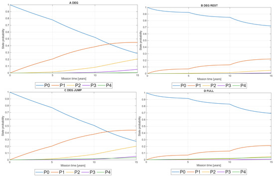
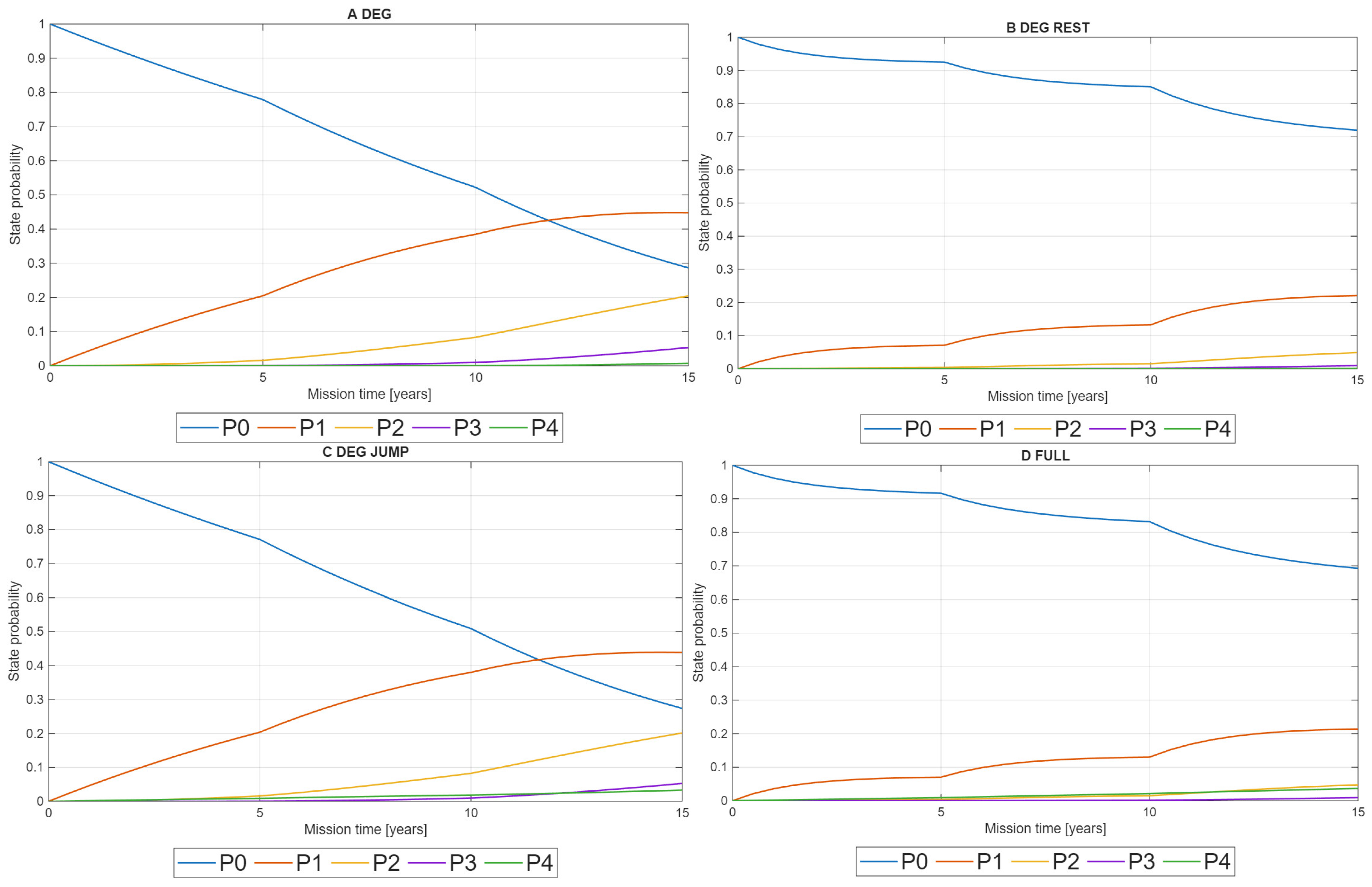
The calculated state-probability trajectories for the four computational variants are presented in Figure 5. All variants start from the fully functional state S0, but their subsequent evolution differs substantially depending on the mechanisms enabled in the model.

Figure 5. State-probability trajectories of the GEO satellite for the four computational variants.

In Variant A—DEG, the absence of restoration results in a continuous transfer of probability mass from S0 toward the degraded states. The probability P₀ decreases from 1 at the beginning of the mission to 0.7788 after 5 years, 0.5221 after 10 years, and 0.2865 after 15 years. At the same time, P1 becomes the largest of the degraded-state probabilities, reaching approximately 0.4482 at the end of the mission. The probabilities P₂ and P₃ also increase, whereas P₄ remains comparatively low because the only path to S4 is the complete sequential sequence S0 → S1 → S2 → S3 → S4.

Variant B—DEG + REST demonstrates the effect of introducing functional restoration while retaining the same sequential degradation structure. Restoration transitions substantially increase the probability of remaining in S0. After 15 years, P₀ equals 0.7198, compared with 0.2865 in Variant A. Probability accumulation in S1–S3 is correspondingly reduced, while P₄ remains very low at 0.00128. The comparison between Variants A and B therefore isolates the influence of functional restoration and shows that repeated recovery to S0 can substantially change the long-term distribution of functional states even when the degradation intensities remain unchanged.

A different behaviour is observed for Variant C—DEG + JUMP. Introducing the direct S0 → S4 transition produces an immediate probability flow into the critical state that is absent from Variant A. Consequently, P₄ increases progressively and reaches 0.03323 after 15 years. The trajectories of P₀–P₃ remain relatively close to those obtained for Variant A, showing that the principal effect of λ₅ is not a fundamental modification of sequential degradation dynamics but the introduction of an additional route to critical loss of mission capability.

Variant D—FULL combines sequential degradation, the direct S0 → S4 transition, and functional restoration. The probability P₀ remains considerably higher than in Variant C and equals 0.6926 after 15 years. The probabilities P₁, P₂, and P₃ are simultaneously reduced to 0.2140, 0.0474, and 0.00925, respectively. These results demonstrate the strong influence of restoration on the probability distribution of the non-critical functional states.

An important feature is observed for the critical state S4. After 15 years, P₄ equals 0.03671 in Variant D, slightly exceeding the value of 0.03323 obtained for Variant C. This result does not indicate a numerical inconsistency. In the full model, restoration transitions repeatedly return probability mass from degraded states to S0. The restored system is subsequently exposed again to the direct S0 → S4 transition governed by λ₅. At the same time, the relatively low μ₄ intensity limits the rate at which probability accumulated in S4 can return to S0. The interaction between these two mechanisms explains why improved preservation of full functional capability does not necessarily imply a monotonically lower instantaneous probability of S4.

The changes in trajectory slopes around years 5 and 10 are associated with the segmented parameterization of the mission. At these boundaries, degradation intensities increase and restoration intensities decrease according to the reference scenario. The resulting trajectories therefore reflect not only elapsed mission time but also the assumed progression of aging and the reduced effectiveness of functional restoration during later mission phases.

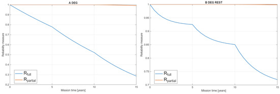
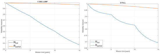
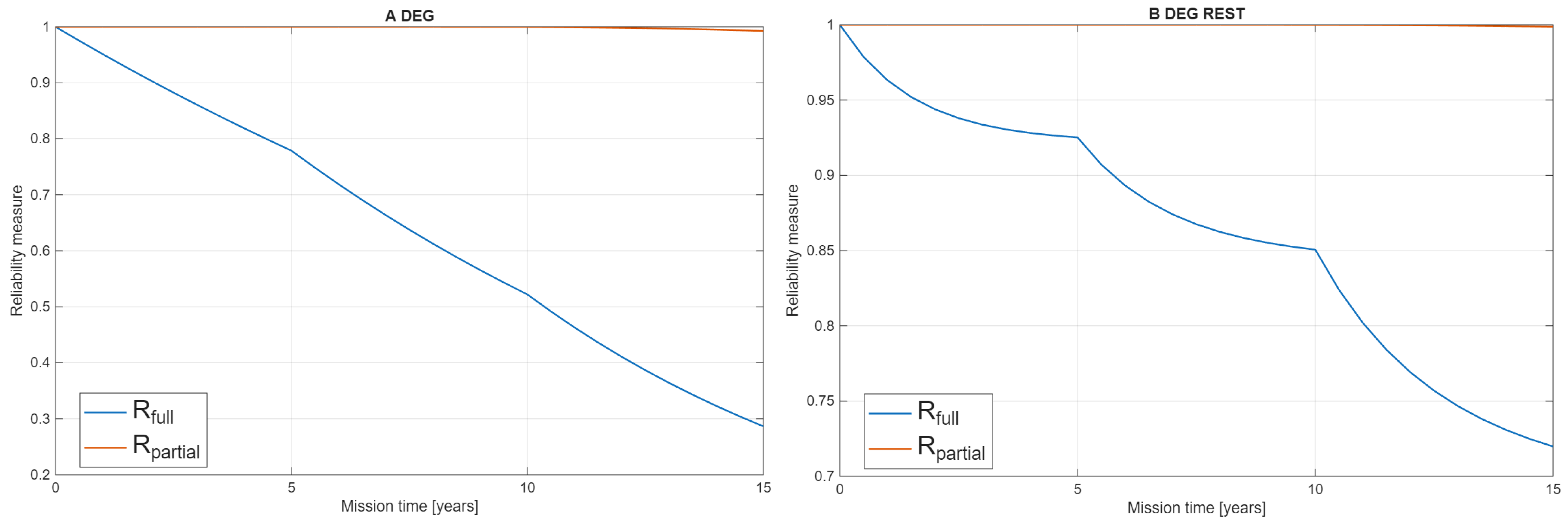
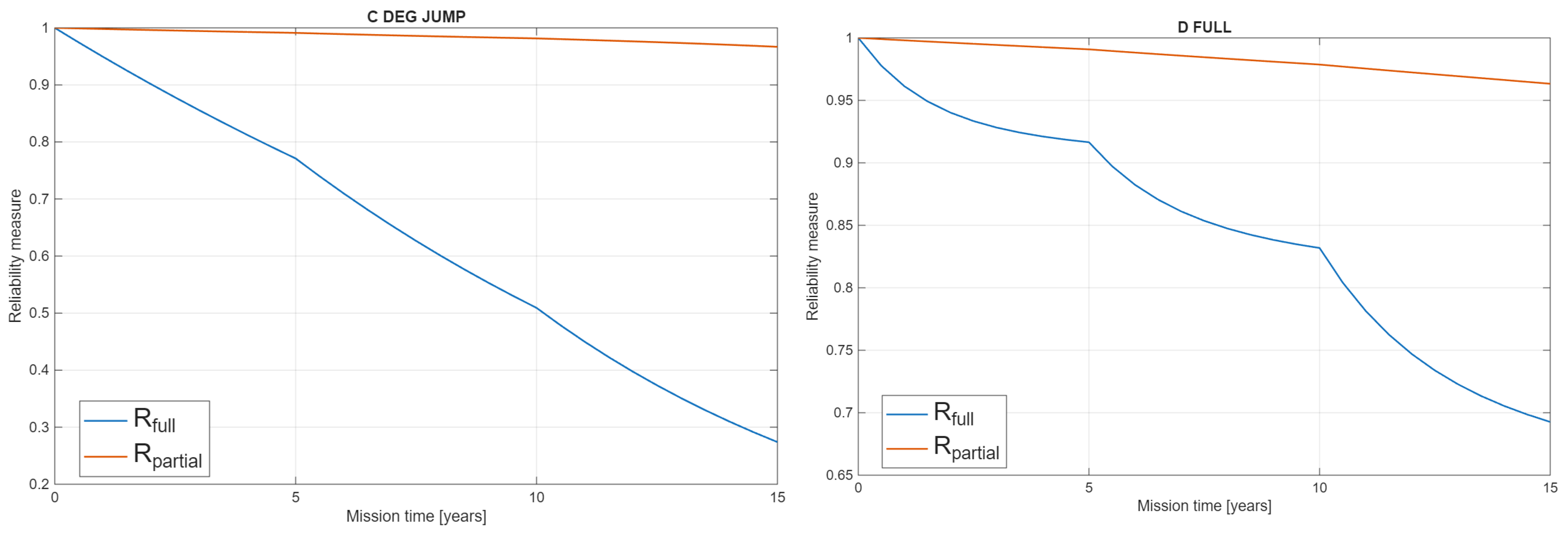
The distinction between full and retained functional capability is shown more clearly in Figure 6.

Figure 6. Full and partial functional capability measures of the GEO satellite for the four computational variants.

For Variant A, Rfull decreases continuously to 0.2865 after 15 years, whereas R_partial remains at 0.9926. This large difference results directly from the five-state interpretation. Although the probability of remaining in S0 becomes relatively low, most probability mass is retained within S1–S3, which represent degraded but still functionally capable states. The result illustrates why a binary reliability representation based only on full operability and failure would not distinguish between loss of nominal performance and loss of critical mission capability.

The effect is even more pronounced in Variant B. Functional restoration maintains R_full at 0.7198 after 15 years, while R_partial remains at 0.9987. Thus, for the sequential-degradation model, functional restoration primarily affects the probability of maintaining full capability rather than the probability of avoiding S4, because reaching the critical state through the complete sequential path remains relatively unlikely within the analysed mission horizon.

The introduction of λ₅ changes this relationship. In Variant C, R_partial decreases to 0.9668 after 15 years, while R_full reaches 0.2739. The direct transition S0 → S4 therefore has a relatively limited effect on the general decline of P₀ but a clearly visible effect on the probability of retaining mission capability outside the critical state. Over the 15-year mission horizon, the cumulative probability of entering S4 in Variant C equals 0.033227. Decomposition of the probability flow shows that 0.025861, corresponding to 77.8%, results from the direct S0 → S4 transition, whereas 0.007366, or 22.2%, results from the sequential S3 → S4 degradation path. Thus, within the adopted reference scenario, sudden critical transitions constitute the dominant mechanism leading to S4. This decomposition refers exclusively to the transition mechanisms represented in the adopted model and does not account for external or mission-specific critical events not captured by the assumed transition intensities.

Variant D provides the most complete representation of the competing mechanisms. Functional restoration maintains R_full at 0.6926 after 15 years, considerably above the value obtained for Variant C, while R_partial equals 0.9633. The increase in P₄ from 0.03323 in Variant C to 0.03671 in Variant D corresponds to 10.47%. The sensitivity analysis shows that P₄ is substantially more responsive to λ₅ than to μ₄: a ±10% change in λ₅ changes P₄ from 0.03323 to 0.04018, whereas the same relative change in μ₄ changes P₄ only from 0.03687 to 0.03654. This confirms that restoration increases repeated exposure to the direct S0 → S4 transition, while μ₄ only partially offsets the resulting probability accumulation in S4. The simultaneous comparison of R_full and R_partial demonstrates that restoration and sudden critical transitions affect different aspects of system behaviour. Restoration strongly supports the preservation of the fully functional state, whereas λ₅ primarily governs the risk of bypassing intermediate degradation states and entering S4 directly.

The separation of these two measures is therefore important for the functional interpretation of GEO satellite reliability. R_full quantifies the probability of maintaining unrestricted mission capability, whereas R_partial quantifies the probability that the satellite remains outside the state associated with loss of critical mission functionality. The difference between these quantities represents the probability mass contained in S1–S3 and consequently provides information about continued operation under degraded conditions that is not available from a two-state representation.

The cumulative state-residence results provide an additional temporal perspective on the full model. For Variant D, the expected cumulative residence time over the 15-year mission horizon equals approximately 12.72 years in S0, 1.78 years in S1, 0.223 years in S2, 0.0286 years in S3, and 0.246 years in S4. The short cumulative residence time in S3 is particularly relevant because S3 represents the pre-critical functional condition immediately preceding sequential transition to S4. Its low residence time results from the combination of the outgoing degradation transition toward S4 and the restoration transition toward S0. However, the operational significance of S3 cannot be assessed solely from its residence time; it also depends on its role as an identifiable pre-critical condition within the state-transition structure. It should also be emphasized that the value of 0.0286 years represents an expected cumulative residence time over the complete 15-year mission horizon rather than a guaranteed continuous warning interval preceding entry into S4. The practical usefulness of S3 for intervention therefore depends on mission-specific telemetry sampling, detection latency, FDIR response time, and operational decision procedures.

5. Discussion

The purpose of this study was to determine whether a five-state functional representation can distinguish mechanisms that are usually combined within a single reliability trajectory of a GEO satellite. The obtained results show that sequential degradation, sudden critical transitions, and functional restoration can be considered separately within the same state structure. The contribution of the proposed approach therefore lies not in a new Markov formalism, but in the functional interpretation of the five states and in the possibility of identifying the individual influence of different degradation and recovery mechanisms.

A relevant feature of the model is the distinction between full mission capability and retained mission capability. The intermediate states S1–S3 represent different levels of degradation without automatically classifying the satellite as failed. Collapsing S1–S3 into a single operational or degraded state, as in conventional two- or three-state representations, would remove the distinction between minor, moderate, and pre-critical degradation that constitutes the diagnostic objective of the present framework. This is particularly important for GEO systems, where degraded operation may remain acceptable and where restoration usually results from redundancy, FDIR, reconfiguration, safe-mode recovery, or software-based actions rather than physical repair. Within this interpretation, S3 represents the last functional state preceding sequential transition to S4 and may therefore provide a useful diagnostic warning condition. Its use as an operational intervention threshold, however, would require mission-specific telemetry and a formally defined decision policy.

The framework can be used for scenario-based reliability assessment and for evaluating how different degradation and restoration assumptions influence long-term mission capability. Because the transition intensities can be replaced without modifying the state structure or computational procedure, the model can also be adapted to specific GEO missions when corresponding operational data become available. Its value is therefore primarily analytical, allowing different degradation and recovery mechanisms to be examined within a common functional classification.

The main limitation of the study is the use of reference rather than satellite-specific transition intensities. Further work should therefore focus on operational parameter identification, uncertainty assessment, and validation using real GEO mission data. An important extension will also involve the interpretation of classical reliability indicators within the five-state functional framework, particularly MTTF as the expected time to first loss of critical mission capability represented by state S4, and MTBF as a measure of the operational cycle between successive losses and restorations of mission capability. This direction may provide reliability indicators that better reflect the multi-state and recoverable nature of long-term satellite operation.

A further limitation is that the segmented CTMC captures mission-age dependence through interval-specific transition intensities but retains the Markov memoryless assumption within each interval. Consequently, it does not reproduce path-dependent degradation history, which would require a semi-Markov or non-Markov aging formulation.

6. Conclusions

This study developed a five-state Markov reliability model for GEO satellites that integrates sequential degradation, direct transition to critical loss of mission capability, and functional restoration. The four computational variants enabled the influence of these mechanisms to be separated and assessed within the same state structure. The distinction between R_full = P₀ and R_partial = 1 − P₄ additionally allowed full mission capability to be distinguished from continued operation in degraded but still functional states.

The results support the usefulness of the five-state classification for representing intermediate degradation and the pre-critical state S3 without treating every departure from S0 as failure. The framework is therefore intended for reliability assessment and scenario analysis and can be parameterized with mission-specific data when such data are available.

The calculations were implemented in MATLAB 2025 using the matrix exponential method and independently verified by numerical integration of the corresponding differential equations. The agreement between both approaches was within approximately 10⁻¹⁴, while probability normalization was maintained within approximately 10⁻¹⁶. The main limitation is the use of reference rather than satellite-specific transition intensities. Further work should therefore focus on operational parameter identification, uncertainty assessment, validation using real GEO mission data, and extension of the framework to MTTF, interpreted as the expected time to first entry into S4, and MTBF, defined with respect to successive losses and restorations of mission capability.

References

- Castet, J.-F.; Saleh, J.H. Satellite and satellite subsystems reliability: Statistical data analysis and modeling. Reliab. Eng. Syst. Saf. 2009, 94, 1718–1728. [Google Scholar] [CrossRef] [Scilit]
- Castet, J.-F.; Saleh, J.H. Beyond reliability, multi-state failure analysis of satellite subsystems: A statistical approach. Reliab. Eng. Syst. Saf. 2010, 95, 311–322. [Google Scholar] [CrossRef] [Scilit]
- Saleh, J.H.; Castet, J.-F. Spacecraft Reliability and Multi-State Failures: A Statistical Approach; John Wiley & Sons: New York, NY, USA, 2011. [Google Scholar] [CrossRef] [Scilit]
- Tafazoli, M. A study of on-orbit spacecraft failures. Acta Astronaut. 2009, 64, 195–205. [Google Scholar] [CrossRef] [Scilit]
- Dubos, G.F.; Castet, J.-F.; Saleh, J.H. Statistical reliability analysis of satellites by mass category: Does spacecraft size matter? Acta Astronaut. 2010, 67, 584–595. [Google Scholar] [CrossRef] [Scilit]
- Haga, R.A.; Saleh, J.H. Epidemiology of satellite anomalies and failures: A subsystem-centric approach. Acta Astronaut. 2011, 69, 676–690. [Google Scholar] [CrossRef] [Scilit]
- Kim, S.Y.; Castet, J.-F.; Saleh, J.H. Spacecraft electrical power subsystem: Failure behavior, reliability, and multi-state failure analyses. Reliab. Eng. Syst. Saf. 2012, 98, 55–65. [Google Scholar] [CrossRef] [Scilit]
- Wayer, J.K.; Castet, J.-F.; Saleh, J.H. Spacecraft attitude control subsystem: Reliability, multi-state analyses, and comparative failure behavior in LEO and GEO. Acta Astronaut. 2013, 85, 83–92. [Google Scholar] [CrossRef] [Scilit]
- Choi, H.-S.; Lee, J.; Cho, K.-S.; Kwak, Y.-S.; Cho, I.-H.; Park, Y.-D.; Kim, Y.-H.; Baker, D.N.; Reeves, G.D.; Lee, D.-K. Analysis of GEO spacecraft anomalies: Space weather relationships. Space Weather 2011, 9, S06001. [Google Scholar] [CrossRef] [Scilit]
- Saleh, J.H.; Geng, F.; Ku, M.; Walker, M.L.R. Electric propulsion reliability: Statistical analysis of on-orbit anomalies and comparative analysis of electric versus chemical propulsion failure rates. Acta Astronaut. 2017, 139, 141–156. [Google Scholar] [CrossRef] [Scilit]
- Guo, J.; Monas, L.; Gill, E.K.A. Statistical analysis and modelling of small satellite reliability. Acta Astronaut. 2014, 98, 97–110. [Google Scholar] [CrossRef] [Scilit]
- Lisnianski, A.; Levitin, G. Multi-State System Reliability: Assessment, Optimization and Applications; World Scientific: Singapore, 2003. [Google Scholar] [CrossRef] [Scilit]
- Lin, Y.-H.; Li, Y.-F.; Zio, E. Integrating Random Shocks into Multi-State Physics Models of Degradation Processes for Component Reliability Assessment. IEEE Trans. Reliab. 2015, 64, 154–166. [Google Scholar] [CrossRef] [Scilit]
- Li, X.-Y.; Huang, H.-Z.; Li, Y.-F.; Zio, E. Reliability assessment of multi-state phased mission system with non-repairable multi-state components. Appl. Math. Model. 2018, 61, 181–199. [Google Scholar] [CrossRef] [Scilit]
- Li, X.-Y.; Xiong, X.; Guo, J.; Huang, H.-Z.; Li, X. Reliability assessment of non-repairable multi-state phased mission systems with backup missions. Reliab. Eng. Syst. Saf. 2022, 223, 108462. [Google Scholar] [CrossRef] [Scilit]
- Tipaldi, M.; Bruenjes, B. Survey on Fault Detection, Isolation, and Recovery Strategies in the Space Domain. J. Aerosp. Inf. Syst. 2015, 12, 235–256. [Google Scholar] [CrossRef] [Scilit]
- Bieber, M.; Verhagen, W.J.C.; Cosson, F.; Santos, B.F. Generic Diagnostic Framework for Anomaly Detection—Application in Satellite and Spacecraft Systems. Aerospace 2023, 10, 673. [Google Scholar] [CrossRef] [Scilit]
- Shao, R.; You, W.; Nie, Y. Reliability modeling framework of satellite constellation based on three-parameter interval grey number Lz transformation. Sci. Rep. 2025, 15, 21022. [Google Scholar] [CrossRef] [Scilit] [PubMed]
- Wander, A.; Förstner, R. Model-Based Fault Detection and Diagnosis for Spacecraft with an Application for the SONATE Triple Cube Nano-Satellite. Aerospace 2019, 6, 105. [Google Scholar] [CrossRef] [Scilit]
- Woźniak, M.; Duer, S.; Kulawińska, B.; Gubarevych, O.; Bernatowicz, D. A Continuous-Time Degradation Model for Autonomous Underwater Vehicles with Data-Driven Mission Decision Rules. Appl. Sci. 2025, 15, 12533. [Google Scholar] [CrossRef] [Scilit]
Disclaimer/Publisher’s Note: The statements, opinions and data contained in all publications are solely those of the individual author(s) and contributor(s) and not of MDPI and/or the editor(s). MDPI and/or the editor(s) disclaim responsibility for any injury to people or property resulting from any ideas, methods, instructions or products referred to in the content. |
© 2026 by the authors. Licensee MDPI, Basel, Switzerland. This article is an open access article distributed under the terms and conditions of the Creative Commons Attribution (CC BY) license.