Dynamic RCS-Based Deep Reinforcement Learning Path Planning for Fixed-Wing UAVs in Complex Environments

Abstract

This paper investigates the low-altitude penetration path planning problem for a fixed-wing UAVs in complex battlefield environments with mountainous terrain and radar threats. First, a radar detection probability model and a dynamic radar cross section (RCS) model are established to characterize target exposure risk. Then, a deep reinforcement learning-based (DRL) path planning framework is developed, in which the Soft Actor-Critic (SAC) algorithm is employed to solve the penetration task under dynamic RCS constraints. A multi-objective reward design is constructed to jointly account for target-reaching progress, radar-threat avoidance, obstacle avoidance, and terminal task completion. Simulations show dynamically feasible flight paths under the adopted models. HIL tests conducted in the corresponding five-radar and two-radar numerical scenarios support onboard path planning, waypoint transmission, and functional closed-loop execution. Comparisons reveal a trade-off among penetration time, modeled radar exposure, and computation, with SAC achieving the shortest mean penetration time among successful trials.

1. Introduction

The nature of modern warfare is undergoing profound transformations, with unmanned aerial vehicles (UAVs) emerging as a new form of combat force. Their application scope and operational effectiveness continue to expand. However, with the rapid advancement of air defense technologies, the battlefield environment has become increasingly complex. UAVs now face multiple threats, including radar detection, artillery fire, and missile attacks [1]. Traditional flight modes are no longer sufficient to meet the demands of modern warfare. Therefore, research on UAV penetration technologies in complex, multi-threat environments is of significant practical importance.

In UAV penetration missions, path planning is a core enabling technology for ensuring the safe and efficient penetration of enemy defense systems [2]. Its primary objective is to generate a feasible flight path from the initial point to the target point while simultaneously satisfying three fundamental requirements, namely safety, efficiency, and feasibility. Specifically, the planned path should avoid threats such as enemy radar detection, artillery interception, missile attacks, and static obstacles including terrain and buildings; minimize flight distance and mission time to improve mission-time efficiency while ensuring safety; and comply with the UAV’s dynamic constraints, such as maximum speed, maximum acceleration, and turning radius.

Path planning methods can be broadly categorized into the following approaches: sampling-based methods, such as Rapidly-exploring Random Trees (RRT); search-based methods, such as A*; swarm-intelligence-based optimization methods, such as Particle Swarm Optimization (PSO) [3], Genetic Algorithm (GA), and Ant Colony Optimization (ACO); mathematical optimization methods, such as optimal control algorithms; and machine-learning-based methods, such as reinforcement learning algorithms.

Among these approaches, traditional model-based and heuristic path planning methods have been widely applied to rapid traversal tasks and path planning in complex environments, but they still exhibit several limitations. To address the safe penetration path planning problem for stealth UAVs in multi-radar threat environments, Zhang et al. [4] proposed a modified A* algorithm. The proposed method simultaneously considers kinematic principles, the dynamic radar cross-section (RCS) of stealth UAVs, and networked radar systems. By introducing a radar threat estimation function and a three-dimensional bidirectional sector multi-layer variable-step search strategy into the traditional A* algorithm, an improved A* method was developed to satisfy the requirements of waypoint accuracy and search efficiency. Yang et al. [5] investigated UAV trajectory optimization in complex penetration combat environments by proposing a dynamic RCS threat model and integrating the hp-adaptive-Radau pseudo-spectral method with the receding horizon control algorithm to minimize flight time and cumulative threat probability. Fu et al. [6] introduced a homotopy optimization framework for multi-UAV trajectories. Their framework addresses the dynamic penetration mission planning (PMP) problem through a variable-time mechanism, Gaussian probability field modeling, a hybrid adaptive obstacle avoidance method, and a penetration strategy algorithm. Lim et al. [7] addressed the issue of fixed-wing aircraft potentially entering inevitable collision states (ICSs) in steep mountainous environments by designing paths that begin and end with safe periodic (circular) trajectories, thereby ensuring safety throughout the entire path. Luo et al. [8] proposed an improved three-dimensional path planning algorithm based on comprehensive particle swarm optimization by jointly considering terrain threats, radar detection, and penetration time. However, many of these methods do not account for dynamic changes in the radar cross-section (RCS) of UAVs during penetration. When dynamic RCS is included, the resulting nonconvex optimization can increase solution time and complicate real-time implementation, depending on the formulation and solver.

Energy-aware reference generation is distinct because mission time and path length do not measure fixed-wing propulsion energy. Bianchi et al. [9] combined minimum-energy references with rule-based tracking, while Yuan et al. [10] accounted for turning-related energy costs. These studies separate explicit energy optimization from the mission-time and modeled radar-exposure objective used here.

MPC and NMPC provide constraint-aware online guidance through receding-horizon optimization. Chen et al. [11] applied NMPC to fixed-wing carrier landing under disturbances, control saturation, safety constraints, and fuel-related objectives. Dynamic-RCS penetration would additionally require online threat estimates and a nonconvex constrained solution at each update. This can increase computational burden and sensitivity to model and solver settings.

To overcome the limitations of traditional path planning methods, reinforcement-learning-based path planning methods have attracted increasing attention in recent years [12,13]. Reinforcement learning can be used to solve optimal control problems under various constraints. In reinforcement learning, an agent interacts with an environment containing multiple threats and learns to generate paths that satisfy UAV dynamic constraints by maximizing the cumulative reward. RL leverages function approximation methods, such as neural networks, to effectively handle high-dimensional state spaces and optimize highly nonlinear and nonconvex objectives. Alpdemir [14] proposed a deep reinforcement learning method for UAV path planning under enemy radar tracking, which alleviates the sparse-reward problem and improves the performance of the learning agent. Xue and Chen [15] formulated the constrained UAV navigation problem as a partially observable Markov decision process (POMDP) and developed a fast recursive stochastic value gradient algorithm based on an actor–critic framework, enabling safe UAV navigation in unknown, complex, and large-scale environments. Xi et al. [16] proposed a lightweight real-time trajectory planning method for UAVs in complex urban environments, termed the Adaptive Trajectory Planning (ASAC) algorithm, and demonstrated its strong robustness and generalization capability.

Recent work also combines reinforcement learning with attitude-dependent radar exposure. Bao et al. [17] considered two-dimensional constant-speed planning with dynamic RCS, multiple radars, DDQN, and five discrete steering actions. Their validation was limited to numerical simulation. Li et al. [18] formulated radar-evasive UCAV trajectory planning as a POMDP and used continuous control with a history-aware, attention-based ME-TD3 policy. These studies indicate that several key components relevant to the present problem, including dynamic RCS modeling, DRL-based radar-evasive planning, continuous control, partial observability, and attitude–RCS coupling, have already been explored in the recent literature.

Despite the progress achieved by both traditional optimization-based methods and reinforcement-learning-based methods, several critical issues remain unresolved in dynamic-RCS-aware penetration path planning. First, in most UAV penetration path planning studies, the radar cross-section (RCS) is either neglected or treated as a constant [19]. Although this approach greatly reduces the complexity of the optimization problem, it overlooks the fact that a UAV’s radar detection probability is positively correlated with its RCS. Dynamic changes in RCS during UAV flight significantly affect radar detection probability, and treating RCS as a constant can therefore substantially alter the optimization results of penetration tasks. Although some studies have considered dynamic changes in RCS, the resulting high-order nonlinearity and nonconvexity of the optimization objectives often lead to high computational complexity and long optimization times [20].

Motivated by the above limitations, this paper proposes a deep-reinforcement-learning-based path planning framework for fixed-wing UAVs. The SAC policy serves as a high-level path planner. Its load-factor and roll-angle outputs are used to propagate the kinematic planning model and generate a dynamically feasible path rather than actuator commands. The resulting path is represented as a waypoint sequence for execution by the low-level flight controller. Dynamic RCS is incorporated into radar-detection estimation to account for modeled exposure during path planning. Therefore, the novelty of this study lies not in any single component alone, but in the specific integration of SAC-based high-level path planning, current partial observations, attitude–RCS-coupled radar-risk evaluation, three-dimensional fixed-wing kinematic propagation, and PX4-based HIL implementation. The contributions of this paper are summarized as follows:

(1)

A dynamic radar cross-section (RCS) model is incorporated into radar detection probability estimation for fixed-wing UAVs, and the objective function is optimized based on this dynamic characteristic to effectively reduce radar detection probability for three-dimensional penetration planning.

(2)

To improve mission performance, the Soft Actor-Critic (SAC) algorithm is adopted to achieve end-to-end path planning with attitude coupling for fixed-wing UAVs in radar environments.

(3)

Numerical experiments characterize the method’s trade-offs with benchmarks in penetration time, modeled radar exposure, and computation time, while corresponding HIL scenarios examine onboard path planning and closed-loop waypoint execution.

2. Problem Formulation and Threat Modeling

2.1. Fixed-Wing UAV Kinematic Model

This paper considers the path planning and control problem of a fixed-wing UAV in three-dimensional space. For translational motion, the fixed-wing UAV is approximated as a particle moving in three-dimensional space, which enables a tractable description of its path evolution. It should be noted that this particle assumption is adopted only for the kinematic modeling of the UAV motion, whereas the attitude-related variables are retained for radar cross-section (RCS) evaluation, since the dynamic RCS depends on the relative orientation between the UAV body and the incident radar wave. By neglecting aerodynamic disturbances and sideslip effects, the kinematic equations of the fixed-wing UAV in the ground-based inertial coordinate system can be written as follows [21]:

$$\left\{\begin{array}{cc}\hfill {\displaystyle \frac{dx}{dt}}& =V\cos \vartheta \cos \psi ,\hfill \\ \hfill {\displaystyle \frac{dy}{dt}}& =V\cos \vartheta \sin \psi ,\hfill \\ \hfill {\displaystyle \frac{dz}{dt}}& =V\sin \vartheta ,\hfill \\ \hfill {\displaystyle \frac{dV}{dt}}& =g(N_x-\sin \vartheta ),\hfill \\ \hfill {\displaystyle \frac{d\vartheta }{dt}}& ={\displaystyle \frac{g}{V}}(N_z\cos \phi -\cos \vartheta ),\hfill \\ \hfill {\displaystyle \frac{d\psi }{dt}}& ={\displaystyle \frac{g{N}_z\sin \phi }{V\cos \vartheta }},\hfill \end{array}\right.$$

(1)

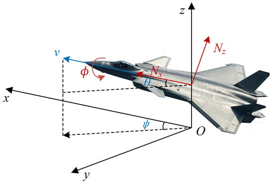
where ${[x,y,z]}^T$ denotes the three-dimensional position of the fixed-wing UAV in the inertial coordinate system, and V denotes the UAV speed. The variables $\psi$ and $\vartheta$ represent the heading angle and flight-path angle, respectively, while $N_x$, $N_z$, and $\phi$ denote the tangential load factor, normal load factor, and roll angle, respectively. The policy outputs an incremental normal-load-factor command $\Delta N_z\in [-0.2,0.2]$ relative to the 1g trim condition. The kinematic equations use the total value $N_z=1+\Delta N_z\in [0.8,1.2]$, so level flight corresponds to $N_z\approx 1$. The state vector of the model at time t is $\mathbf{X}\left(t\right)={[x,y,z,V,\vartheta ,\psi ]}^T$, and the control vector is $\mathbf{U}\left(t\right)={[N_x,N_z,\phi ]}^T$. The relationship between the coordinate systems and the associated angular variables of the fixed-wing UAV is illustrated in Figure 1.

Figure 1. The model of fixed-wing UAVs.

2.2. Dynamic-RCS-Based Radar Detection Model

2.2.1. Radar Detection Probability Model

For a single radar system, assuming that the radar performance parameters are known, the detection probability of a fixed-wing UAV depends only on the Euclidean distance between the UAV and the radar, as well as the radar cross-section (RCS) of the UAV. The detection probability for a single radar is given by [22]

$$P_{\mathrm{d}}=\left\{\begin{array}{cc}\exp \left({\displaystyle \frac{C_d{R}_i^4}{\sigma }}\right),\hfill & R_i\le R_{\det };\hfill \\ 0,\hfill & otherwise,\hfill \end{array}\right.$$

(2)

where $R_i$ denotes the radar–UAV distance expressed in kilometers, $\sigma$ denotes the UAV RCS expressed in square meters, and $R_{\det }$ denotes the maximum radar detection range. Accordingly, $C_d$ has units of ${\mathrm{m}}^2 {\mathrm{km}}^{-4}$, ensuring that $C_d{R}_i^4/\sigma$ is dimensionless. In this paper, $C_d$ is treated as a fixed planning-level modeling coefficient rather than a physically calibrated parameter of a specific radar system.

In complex battlefield environments, multiple radars are often deployed as a network to improve the detection capability against fixed-wing UAVs. The detection probability of the radar network can be expressed as follows:

$$P_{\mathrm{D}}=1-{\displaystyle \prod _{j=1}^m}(1-P_{\mathrm{d},j}),$$

(3)

where j is the radar index, $P_{\mathrm{d},j}$ denotes the detection probability of the j-th radar, and m denotes the total number of radars.

2.2.2. Dynamic RCS Model of Fixed-Wing UAVs

The RCS of a fixed-wing UAV is a crucial factor influencing the radar detection probability. In general, the RCS varies with the direction of the incident radar wave, and an omnidirectional minimum RCS is rarely achieved. The following parametric RCS model is adopted [23]:

$$\sigma (\alpha ,\beta )=k_1+k_2\sin \alpha +k_3|\sin \alpha \sin (2\beta +{\displaystyle \frac{\pi }{2}})|,$$

(4)

where $\alpha$ and $\beta$ denote the azimuth angle and polar angle in the spherical coordinate system, respectively, and are used to characterize the spatial angular relationship of the UAV relative to the radar incident direction. The parameters $k_1$, $k_2$, and $k_3$ are the fitting coefficients of the radar cross-section (RCS) curve. Specifically, $k_1$ represents the baseline scattering level independent of attitude, $k_2$ characterizes the amplitude of directional fluctuation induced by the azimuth angle $\alpha$, and $k_3$ represents the contribution amplitude of the coupling term between the azimuth angle $\alpha$ and the polar angle $\beta$ to the RCS fluctuation. These three parameters are engineering fitting parameters, and their values depend on factors such as target shape, operating frequency band, and polarization. Simulations use $(k_1,k_2,k_3)=(1.01,0.99,10)$ from the parameterization in [23]. Because the source omits radar frequency, polarization, calibration data, and fitting uncertainty, this planning-level model is not calibrated to the HIL airframe.

For any point $(\xi ,\eta ,\zeta )$ in the Cartesian coordinate system, the corresponding spherical coordinates $(\rho ,\alpha ,\beta )$ can be obtained through the following transformation:

$$\left\{\begin{array}{cc}\hfill \rho & =\sqrt{{\xi }^2+{\eta }^2+{\zeta }^2},\hfill \\ \hfill \beta & =\arccos \left({\displaystyle \frac{\zeta }{\rho }}\right),\hfill \\ \hfill \alpha & =\mathrm{atan2}\left(\eta ,\xi \right),\hfill \end{array}\right.$$

(5)

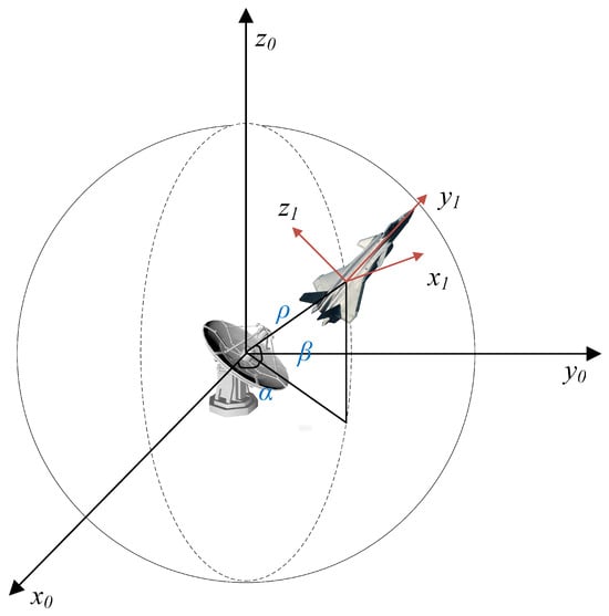
where $\rho$ denotes the radial distance from the point to the origin of the coordinate system. $\beta \in [0,\pi ]$ describes the angular position of the point in the vertical plane, and $\alpha \in (-\pi ,\pi ]$ represents its azimuth in the horizontal plane. The relative geometric relationship between the radar and the fixed-wing UAV is illustrated in Figure 2.

Figure 2. The relative position of the radars and the fixed-wing UAVs.

According to the parametric radar cross-section (RCS) model, the UAV’s RCS under several specific discrete combinations of the azimuth angle $\alpha$ and polar angle $\beta$ with respect to the radar can be expressed as follows:

$$\sigma =\left\{\begin{array}{cc}{k}_1,\hfill & \alpha =n\pi ,\beta \in [0,\pi ],\hfill \\ k_1+{(-1)}^n{k}_2,\hfill & \alpha ={\displaystyle \frac{(2n+1)\pi }{2}},\beta ={\displaystyle \frac{(2m-1)\pi }{4}},\hfill \\ k_1+\sin \left({\displaystyle \frac{(2n+1)\pi }{4}}\right)k_2,\hfill & \alpha ={\displaystyle \frac{(2n+1)\pi }{4}},\beta ={\displaystyle \frac{(2m-1)\pi }{4}},\hfill \end{array}\right.$$

(6)

where n is an integer.

When $\alpha =n\pi$, the nose or tail of the UAV is aligned with the radar line of sight, and the model gives the baseline value $\sigma =k_1$ rather than the global minimum. When $\alpha =(2n+1)\pi /2$ and $\beta =(2m-1)\pi /4$, the $k_3$ term vanishes and $\sigma =k_1+{(-1)}^n{k}_2$. For even n, this value is $k_1+k_2$, whereas for odd n it is $k_1-k_2$. The global minimum $k_1-k_2=0.02{\mathrm{m}}^2$ occurs at $\alpha =-\pi /2$ and $\beta =\pi /4$ or $3\pi /4$. When $\alpha =(2n+1)\pi /4$ at the same $\beta$ values, $\sigma =k_1+\sin [(2n+1)\pi /4]k_2=k_1\pm \sqrt{2}{k}_2/2$, where the sign is determined by n. The global maximum $k_1+k_2+k_3=12.00{\mathrm{m}}^2$ occurs at $\alpha =\pi /2$ and $\beta =0$, $\pi /2$, or $\pi$. Here, n and m are integers. Thus, Equation (6) gives sign-dependent RCS values and is consistent with the theoretical extrema of Equation (4).

To establish the mapping relationship between the radar incident direction and the UAV attitude, the azimuth angle $\alpha$ and polar angle $\beta$ of the incident direction are computed in the UAV body-fixed frame ${\mathcal{F}}_U$. Let ${\mathcal{F}}_E$ denote the world coordinate frame, and let ${\mathbf{p}}_{\mathrm{rad}}^E$ and ${\mathbf{p}}_{\mathrm{uav}}^E$ denote the positions of the radar and the UAV in ${\mathcal{F}}_E$, respectively. Then, the line-of-sight vector from the UAV to the radar is given by

$${\ell }^E={\mathbf{p}}_{\mathrm{rad}}^E-{\mathbf{p}}_{\mathrm{uav}}^E.$$

(7)

The UAV attitude is described by the roll angle $\phi$, flight-path angle $\vartheta$, and heading angle $\psi$. The direction cosine matrix from the body-fixed frame ${\mathcal{F}}_U$ to the world frame ${\mathcal{F}}_E$ is defined as

$${\mathbf{R}}_E^U={\mathbf{R}}_z\left(\psi \right){\mathbf{R}}_y\left(\vartheta \right){\mathbf{R}}_x\left(\phi \right),$$

(8)

and the line-of-sight vector represented in the body-fixed frame ${\mathcal{F}}_U$ can be written as

$${\ell }^U={\mathbf{R}}_U^E{\ell }^E={\left({\mathbf{R}}_E^U\right)}^{\mathrm{T}}{\ell }^E,$$

(9)

where ${\mathbf{R}}_U^E={\left({\mathbf{R}}_E^U\right)}^{\mathrm{T}}$. The elementary rotation matrices about the three axes are given by

$$\begin{array}{cc}\hfill {\mathbf{R}}_x\left(\phi \right)& =\left[\begin{array}{ccc}1& 0& 0\\ 0& \cos \phi & -\sin \phi \\ 0& \sin \phi & \cos \phi \end{array}\right],{\mathbf{R}}_y\left(\vartheta \right)=\left[\begin{array}{ccc}\cos \vartheta & 0& \sin \vartheta \\ 0& 1& 0\\ -\sin \vartheta & 0& \cos \vartheta \end{array}\right],\hfill \\ \hfill {\mathbf{R}}_z\left(\psi \right)& =\left[\begin{array}{ccc}\cos \psi & -\sin \psi & 0\\ \sin \psi & \cos \psi & 0\\ 0& 0& 1\end{array}\right].\hfill \end{array}$$

(10)

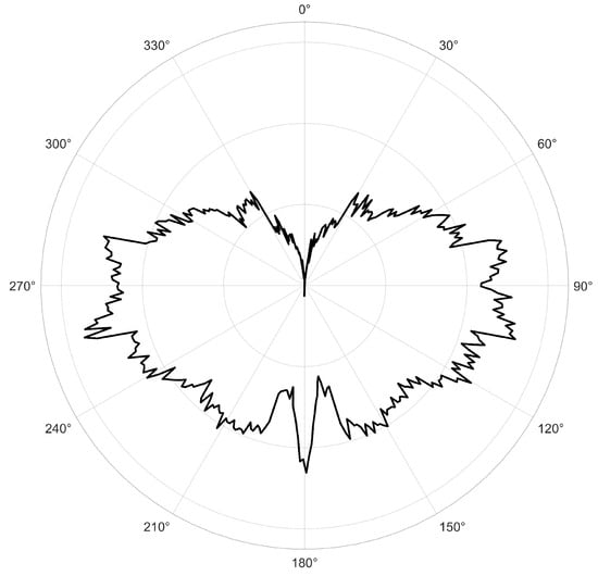
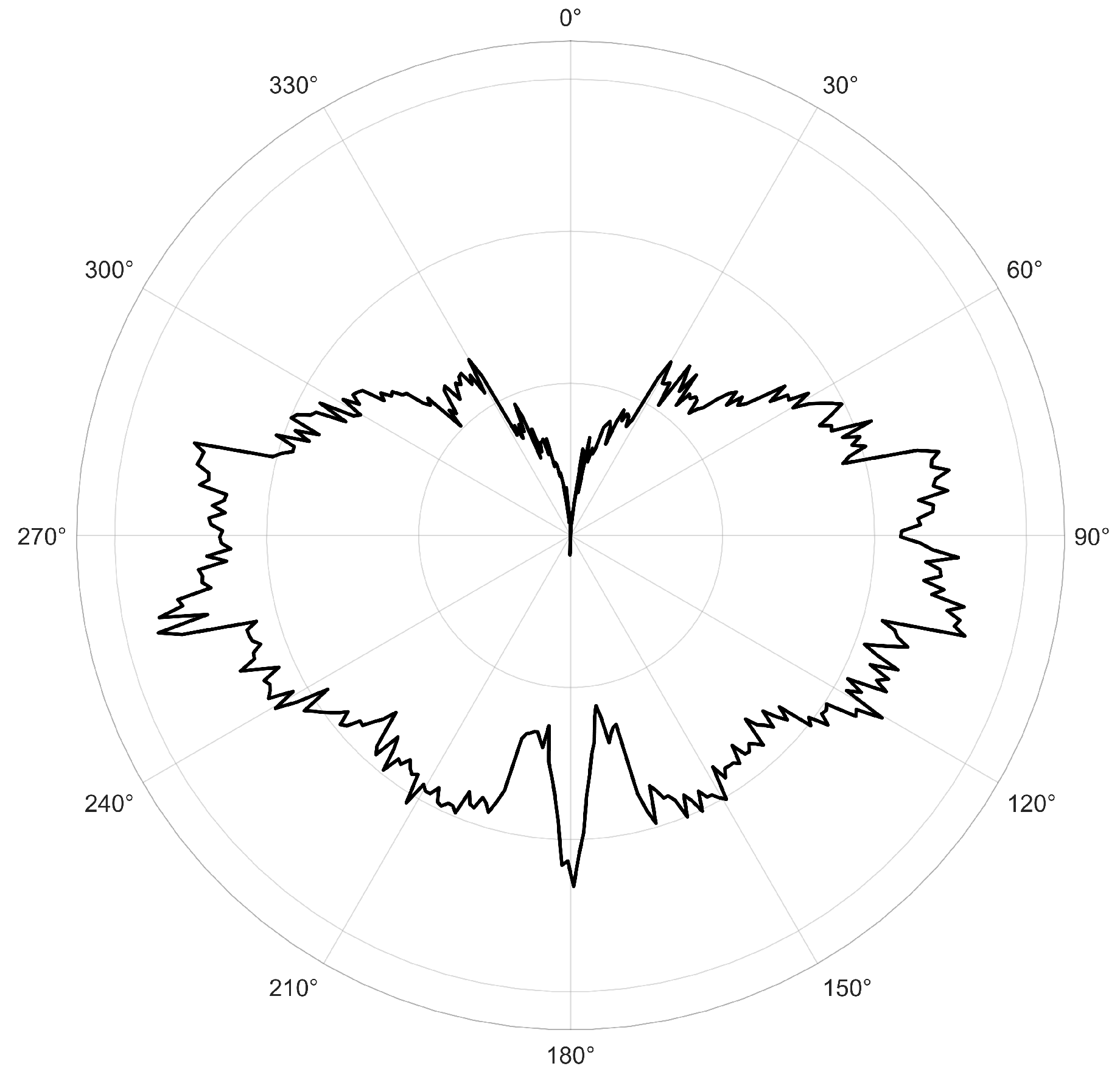
In this way, the radar incident direction can be uniformly represented in the body-fixed frame ${\mathcal{F}}_U$. Subsequently, according to the spherical-coordinate mapping relationship given in (5), the azimuth angle $\alpha$ and polar angle $\beta$ are computed from ${\ell }^U$ and substituted into $\sigma (\alpha ,\beta )$ to complete the dynamic RCS modeling. The relative geometric relationship between the radar and the UAV, as well as the RCS curve of a representative UAV, are shown in Figure 3.

Figure 3. RCS characteristic curve.

2.3. Penetration Task Optimization Model

Based on the mission requirements of fast low-altitude penetration by fixed-wing UAVs, the UAV must reach the designated target as quickly as possible in order to strike time-sensitive targets. Therefore, the time-optimality objective can be expressed as follows:

$$J_t=t_f-t_0,$$

(11)

where $t_0$ and $t_f$ denote the start and end times of the low-altitude penetration mission, respectively. To minimize the radar threat encountered by the fixed-wing UAV during flight, radar detection probability is introduced as another evaluation metric, which can be expressed as follows:

$$J_p={\int }_{t_0}^{t_f}{P}_D(\mathbf{X}\left(t\right),\mathbf{U}\left(t\right))dt.$$

(12)

The objective balances the minimum-time index $J_t$ and cumulative modeled radar-exposure index $J_p$. Then, the optimization problem is defined as

$$\underset{\mathbf{U}\in \mathcal{C}}{\min }J={\int }_{t_0}^{t_f}\mathcal{L}(\mathbf{X}\left(t\right),\mathbf{U}\left(t\right))dt={\int }_{t_0}^{t_f}\left(w_t+w_p{P}_D(\mathbf{X}\left(t\right),\mathbf{U}\left(t\right))\right)dt,$$

(13)

where $\mathcal{C}$ denotes the admissible set of the control input $\mathbf{U}\left(t\right)$. The weights $w_t$ and $w_p$ scale mission time and modeled radar exposure, respectively. Consequently, $\mathcal{L}\left(\mathbf{X}\right(t),\mathbf{U}(t\left)\right)$ defines the running cost function of the unified optimization problem. The continuous-time formulation combines penetration time and cumulative modeled radar exposure in the running cost. Terrain safety is enforced through the admissible set, while target arrival is specified by the terminal constraints. Together, the running cost and constraints define the mission-level penetration problem.

The objective contains no propulsion-energy term or surrogate; mission time and path length are therefore not interpreted as energy measures.

In this paper, the constraints are classified into hard constraints and soft constraints. Hard constraints are conditions that must be strictly satisfied by the solution. Due to the performance limitations of the fixed-wing UAV, the state variables and control variables are all subject to upper and lower bounds. In particular, the flight speed V, the flight-path angle $\vartheta$, the tangential load factor $N_x$, the normal load factor $N_z$, and the roll angle $\phi$ are bounded above and below. The specific numerical values of these bounds are given in the simulation experiments section.

Due to the requirements of the penetration mission, the state variables and control variables of the UAV are generally required to satisfy the following initial and terminal constraints:

$$\left\{\begin{array}{c}\mathbf{x}\left(t_0\right)={\mathbf{x}}_0,\hfill \\ {∥\mathbf{p}\left(t_{\mathrm{f}}\right)-{\mathbf{p}}_{\mathrm{f}}∥}_2\le R_{\mathrm{tol}},\hfill \\ \left|V\left(t_{\mathrm{f}}\right)-V_{\mathrm{f}}\right|\le \Delta V_{\mathrm{tol}},\hfill \\ \left|\vartheta \left(t_{\mathrm{f}}\right)-{\vartheta }_{\mathrm{f}}\right|\le \Delta {\vartheta }_{\mathrm{tol}},\hfill \\ \left|\psi \left(t_{\mathrm{f}}\right)-{\psi }_{\mathrm{f}}\right|\le \Delta {\psi }_{\mathrm{tol}},\hfill \end{array}\right.$$

(14)

where $t_0$ and $t_{\mathrm{f}}$ denote the initial time and terminal time of the mission, respectively; ${\mathbf{x}}_0={\left[x_0,y_0,z_0,V_0,{\vartheta }_0,{\psi }_0\right]}^{\mathrm{T}}$ is the prescribed state vector for the penetration mission; $\mathbf{p}={\left[x,y,z\right]}^{\mathrm{T}}$ denotes the position vector; and ${\mathbf{p}}_{\mathrm{f}}$, $V_{\mathrm{f}}$, ${\vartheta }_{\mathrm{f}}$, and ${\psi }_{\mathrm{f}}$ represent the terminal position, speed, flight-path angle, and heading angle, respectively. In addition, $R_{\mathrm{tol}}$, $\Delta V_{\mathrm{tol}}$, $\Delta {\vartheta }_{\mathrm{tol}}$, and $\Delta {\psi }_{\mathrm{tol}}$ denote the admissible errors in terminal position, speed, flight-path angle, and heading angle, respectively.

Soft constraints, in contrast, correspond to performance indices that the system is expected to optimize. They are incorporated into the objective function J in the form of penalty terms, including the cumulative radar detection probability.

3. Dynamic-RCS-Aware Deep Reinforcement Learning Path Planning

Building on the fixed-wing UAV dynamics and detection models established above, this section proposes a dynamic-RCS-aware deep reinforcement learning algorithm for path planning. To address the nonconvex multi-objective optimization introduced by RCS variability, specialized state representations and reward functions are designed to effectively balance flight time and detection probability.

3.1. POMDP Formulation and SAC-Based Solution

The dynamic RCS-aware low-altitude penetration path planning problem for fixed-wing UAVs can be naturally formulated within a reinforcement learning framework. In principle, such a sequential decision-making problem can be described by a Markov Decision Process (MDP) [24]. However, in practical battlefield environments, the UAV cannot directly access the complete environmental state, especially the exact radar locations and radar operating parameters. Therefore, to more accurately characterize decision making under incomplete information, this problem is modeled as a Partially Observable Markov Decision Process (POMDP) [25].

Formally, a POMDP can be represented by the seven-tuple $<S,A,T,R,\Omega ,O,\gamma >$, where S is the true state space of the environment, A is the action space, $T:S\times A\times S\to [0,1]$ is the state transition function, $R:S\times A\to \mathbb{R}$ is the reward function, $\Omega$ is the observation space, $O:S\times A\times \Omega \to [0,1]$ is the observation function, and $\gamma \in [0,1)$ is the discount factor. Under this framework, the agent cannot directly observe the true environment state $s_t$; instead, it makes decisions based on the available observation $o_t\in \Omega$.

Although history-based representations can address partial observability, this paper uses only current observations as inputs to the policy and value networks. This feedforward implementation does not use memory or state estimation and does not claim that its observations form a sufficient Markov information state.

This paper adopts the Soft Actor-Critic (SAC) algorithm. SAC is an off-policy reinforcement learning algorithm that typically achieves higher sample efficiency than on-policy methods [26]. Compared with DDPG, SAC generally exhibits better convergence behavior and lower sensitivity to hyperparameter tuning, making it more suitable for complex environments. Compared with PPO, SAC further improves sample utilization through the use of an experience replay buffer. Moreover, by incorporating entropy maximization to encourage diverse exploration, SAC achieves improved convergence and stability in continuous-control tasks with highly nonlinear and nonconvex objectives, such as dynamic-RCS-aware UAV path planning.

Entropy is a measure of the uncertainty associated with a random variable. If the probability density function of a random variable x is denoted by $p\left(x\right)$, its entropy $H\left(x\right)$ is defined as

$$H\left(x\right)={\mathbb{E}}_{x\sim p\left(x\right)}[-\log p\left(x\right)].$$

(15)

Within the maximum-entropy reinforcement learning framework, SAC optimizes the policy by maximizing both the expected return and the policy entropy. The resulting optimal policy ${\pi }^{*}$ can be expressed as

$${\pi }^{*}=\arg \underset{\pi }{\max }{\mathbb{E}}_{\pi }\left[\sum _t{r}_t(o_t,a_t)+\kappa H\left(\pi (·|o_t)\right)\right],$$

(16)

where $\pi$ denotes a stochastic policy, $o_t$ and $a_t$ denote the observation and action at time step t, respectively, $r_t(o_t,a_t)$ denotes the immediate reward obtained at time step t, $H\left(\pi (·|o_t)\right)$ denotes the entropy of the policy conditioned on observation $o_t$, and $\kappa$ is the temperature parameter.

The SAC algorithm further introduces entropy-augmented soft action-value and soft state-value functions, defined as

$$\begin{array}{cc}\hfill {\mathcal{Q}}^{\mathrm{soft}}(o_t,a_t)& =r(o_t,a_t)+\gamma {\mathbb{E}}_{o_{t+1}}\left[{\mathcal{V}}^{\mathrm{soft}}\left(o_{t+1}\right)\right],\hfill \\ \hfill {\mathcal{V}}^{\mathrm{soft}}\left(o_t\right)& ={\mathbb{E}}_{a_t}\left[{\mathcal{Q}}^{\mathrm{soft}}(o_t,a_t)-\kappa \log \pi \left(a_t\right|o_t)\right],\hfill \end{array}$$

(17)

where $o_{t+1}$ is sampled from the replay buffer $\mathcal{D}$. ${\mathbb{E}}_{o_{t+1}}[·]$ and ${\mathbb{E}}_{a_t}[·]$ denote the expectations with respect to the environment transition distribution and the policy distribution, respectively.

The neural-network-based implementation of SAC consists of one actor network and two critic networks. The actor network outputs the stochastic policy ${\pi }_{\theta }\left(a_t\left|o_t\right.\right)$, while the critic networks estimate the observation–action value functions ${\mathcal{Q}}_{{\varphi }_i}(o_t,a_t)$, $i=1,2$, where $\theta$ denotes the parameter set of the actor network and ${\varphi }_i$ denotes the parameter set of the i-th critic network. The critic employs a clipped double-$\mathcal{Q}$ structure to alleviate value overestimation, thereby improving training stability.

The loss function of the critic network is defined as

$$L_{\mathcal{Q}}\left({\varphi }_i\right)={\mathbb{E}}_{(o_t,a_t,r_t,o_{t+1})\sim \mathcal{D}}\left[{\displaystyle \frac{1}{2}}{\left(Q_{{\varphi }_i}(o_t,a_t)-y_t\right)}^2\right],i=1,2,$$

(18)

where $L_{\mathcal{Q}}\left({\varphi }_i\right)$ denotes the loss function of the i-th critic network, $\mathcal{D}$ denotes the replay buffer, and $y_t$ denotes the target value. The target value $y_t$ is given by

$$y_t=r_t+\gamma (1-{\delta }_t^{\mathrm{term}})\left(\underset{j=1,2}{\min }{\mathcal{Q}}_{{\varphi }_{\mathrm{targ},j}}(o_{t+1},a_{t+1}^{\prime })-\kappa \log {\pi }_{\theta }\left(a_{t+1}^{\prime }\right|o_{t+1})\right),$$

(19)

where ${\mathcal{Q}}_{{\varphi }_{\mathrm{targ},j}}$ denotes the j-th target critic network, ${\varphi }_{\mathrm{targ},j}$ denotes its parameter set, and $a_{t+1}^{\prime }$ is sampled from the current policy according to

$$a_{t+1}^{\prime }\sim {\pi }_{\theta }(·|o_{t+1}).$$

(20)

The loss function of the actor network is defined as

$$L_{\pi }\left(\theta \right)={\mathbb{E}}_{o_t\sim \mathcal{D}}\left[{\mathbb{E}}_{a_t\sim {\pi }_{\theta }(·|o_t)}\left[\kappa \log {\pi }_{\theta }\left(a_t\right|o_t)-\underset{i=1,2}{\min }{\mathcal{Q}}_{{\varphi }_i}(o_t,a_t)\right]\right].$$

(21)

To automatically adjust the exploration strength, the temperature parameter is optimized by minimizing

$$L\left(\kappa \right)={\mathbb{E}}_{o_t\sim \mathcal{D}}\left[{\mathbb{E}}_{a_t\sim {\pi }_{\theta }(·|o_t)}\left[-\kappa \left(\log {\pi }_{\theta }\left(a_t\right|o_t)+{\mathcal{H}}_{\mathrm{targ}}\right)\right]\right],$$

(22)

where ${\mathcal{H}}_{\mathrm{targ}}$ denotes the target entropy used to automatically tune the exploration intensity.

In this way, the SAC algorithm iteratively updates the actor network, critic networks, and temperature parameter based on partial observations and the sampled transition tuples $(o_t,a_t,r_t,o_{t+1},{\delta }_t^{\mathrm{term}})$, where ${\delta }_t^{\mathrm{term}}\in \{0,1\}$ denotes the termination indicator at time step t, with ${\delta }_t^{\mathrm{term}}=1$ indicating that the fixed-wing UAV collides with the terrain or reaches the target region, and ${\delta }_t^{\mathrm{term}}=0$ otherwise. This enables the UAV to learn an effective penetration policy that accounts for dynamic RCS characteristics.

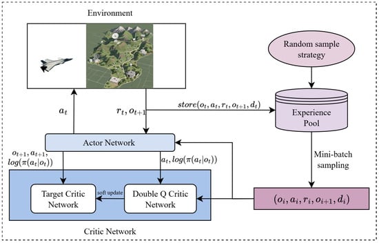
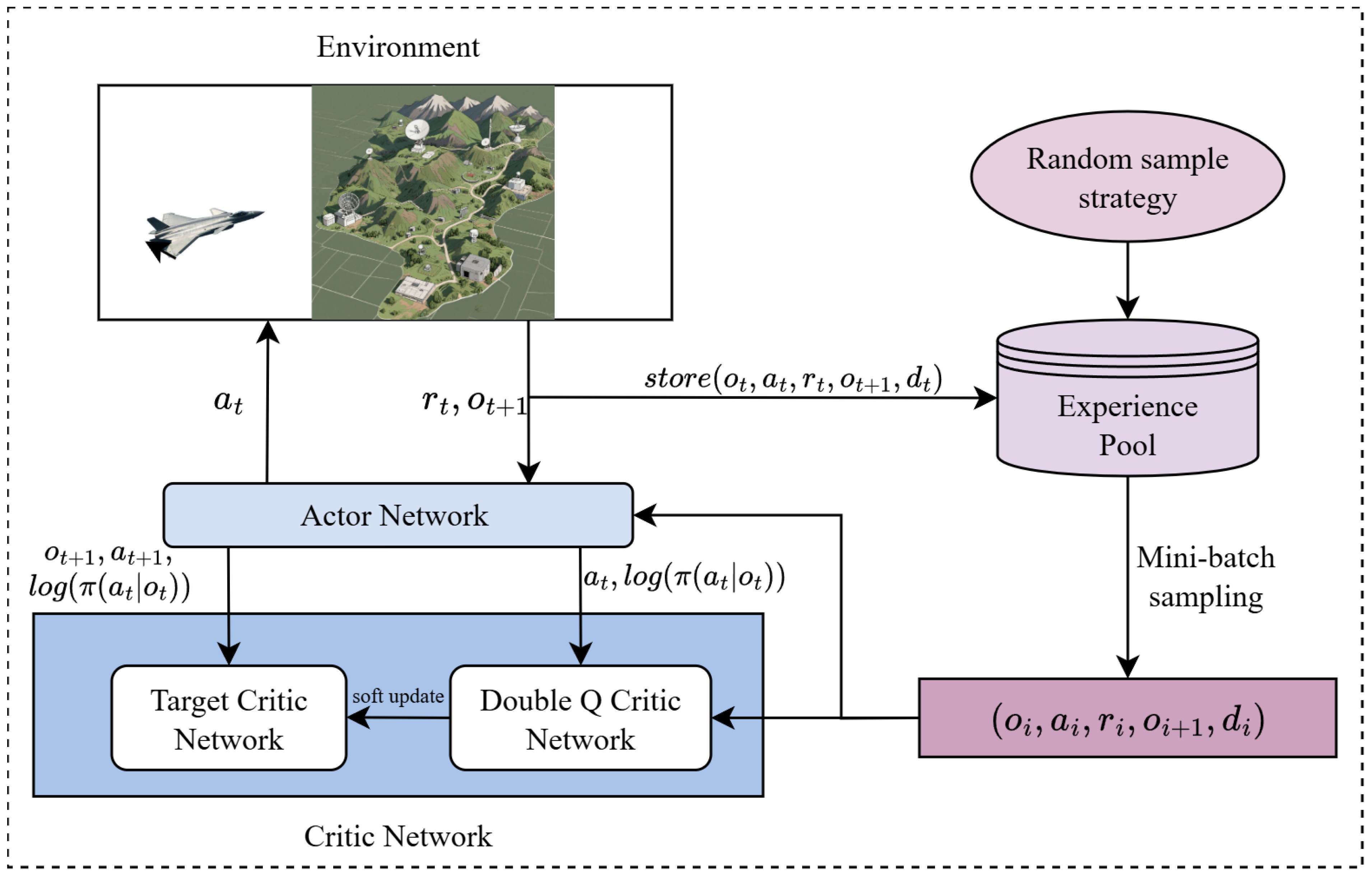
Based on the above problem formulation and SAC-based solution, the overall framework of the proposed reinforcement-learning-based path planning method for fixed-wing UAVs is shown in Figure 4. The framework mainly includes environment modeling, observation construction, policy learning, and path generation. In detail, at each planning step, the bounded SAC action is mapped to the fixed-wing kinematic model to propagate position, velocity, and attitude. The propagated attitude and radar-relative geometry determine the parametric RCS; RCS and range then determine the modeled radar-exposure indicator. Target progress, terrain clearance, modeled radar exposure, and terminal status form the reward returned to SAC. Repeating this interaction produces a dynamically feasible path represented by an ordered sequence of path points, which is subsequently converted into waypoint references for PX4 execution in HIL. Through repeated interaction with the environment, the UAV learns a policy that balances time efficiency and modeled radar-exposure risk under the adopted threat model.

Figure 4. Overall framework of the proposed reinforcement learning-based path planning algorithm.

3.2. Training Configuration for Penetration Planning

3.2.1. State Space

For the low-altitude penetration mission of fixed-wing UAVs in complex environments, the decision-making process should characterize the UAV’s own state, its relative relationship to the target, and radar-threat-related information. Ideally, the true state space can be expressed as

$$\mathbf{s}={\left[\mathbf{X},\mathbf{\Psi },\mathbf{D}\right]}^T,$$

(23)

where $\mathbf{X}={\left[x,y,z,V,\vartheta ,\psi \right]}^T$ denotes the UAV state in the dynamic model; $\mathbf{\Psi }={\left[\Delta {\mathit{d}}_{\mathrm{g}},\Delta \mathit{\varpi }\right]}^T$ describes the relative relationship between the UAV and the target, where $\Delta {\mathit{d}}_{\mathrm{g}}$ is the relative displacement along the three coordinate axes and $\Delta \mathbf{\varpi }$ is the angle between the UAV velocity direction and the target-direction vector; and $\mathbf{D}={\left[{\mathrm{D}}_1,{\mathrm{D}}_2,\dots ,{\mathrm{D}}_m\right]}^T$ denotes the relative distance information between the UAV and the radars, where ${\mathrm{D}}_j$ denotes the relative distance between the UAV and the j-th radar, and m is the total number of radars.

Under the POMDP framework, however, the agent cannot directly access the complete true state. In practice, the UAV’s own state $\mathbf{X}$ can be obtained from the inertial navigation system and GPS, while the goal-related state $\mathbf{\Psi }$ can be derived from geometric relationships. In contrast, the exact radar positions $(p_x^j,p_y^j,p_z^j)$ and their operating parameters are not directly observable, where $j\in 1,2,\dots ,m$. Instead, the UAV can only obtain the direction-of-arrival information of each radar signal, represented in spherical coordinates by the azimuth and polar angles:

$$\begin{array}{cc}\hfill {\mathit{\alpha }}_{\mathrm{radar}}& ={\left[{\alpha }_{\mathrm{radar}}^1,{\alpha }_{\mathrm{radar}}^2,\dots ,{\alpha }_{\mathrm{radar}}^m\right]}^{\mathrm{T}},\hfill \\ \hfill {\mathit{\beta }}_{\mathrm{radar}}& ={\left[{\beta }_{\mathrm{radar}}^1,{\beta }_{\mathrm{radar}}^2,\dots ,{\beta }_{\mathrm{radar}}^m\right]}^{\mathrm{T}},\hfill \end{array}$$

(24)

where ${\alpha }_{\mathrm{radar}}^j\in (-\pi ,\pi ]$ denotes the relative azimuth angle and ${\beta }_{\mathrm{radar}}^j\in [0,\pi ]$ denotes the relative polar angle of the j-th radar with respect to the UAV.

In practical applications, radar-threat information may be estimated from onboard electronic-support or radar-warning systems, such as through passive emitter-localization techniques based on angle-of-arrival, time-difference-of-arrival, or frequency-difference-of-arrival measurements [27,28]. Such sensing mechanisms can provide threat-direction, emitter-location, or warning-level information for onboard planning. In the present study, however, a complete onboard electronic-reconnaissance sensing and fusion chain is not modeled. The radar-direction angles are computed from the modeled radar–UAV relative geometry and UAV attitude. The aggregate modeled radar-detection probability $P_{\mathrm{D}}$ is calculated using the modeled radar configuration, radar ranges, and attitude-dependent RCS model, according to the radar-detection model in Section 2.2.1. Both the radar-direction angles and $P_{\mathrm{D}}$ are supplied by the simulation environment as observation features; they are not obtained through direct onboard measurements. The angles are also used for RCS evaluation, and $P_{\mathrm{D}}$ is used for reward construction and performance evaluation.

The observation vector supplied to the actor is

$$o_t={[{\mathbf{X}}_t,{\mathbf{\Psi }}_t,{\mathit{\alpha }}_{\mathrm{radar},t},{\mathit{\beta }}_{\mathrm{radar},t},P_{\mathrm{D},t}]}^{\mathrm{T}}.$$

(25)

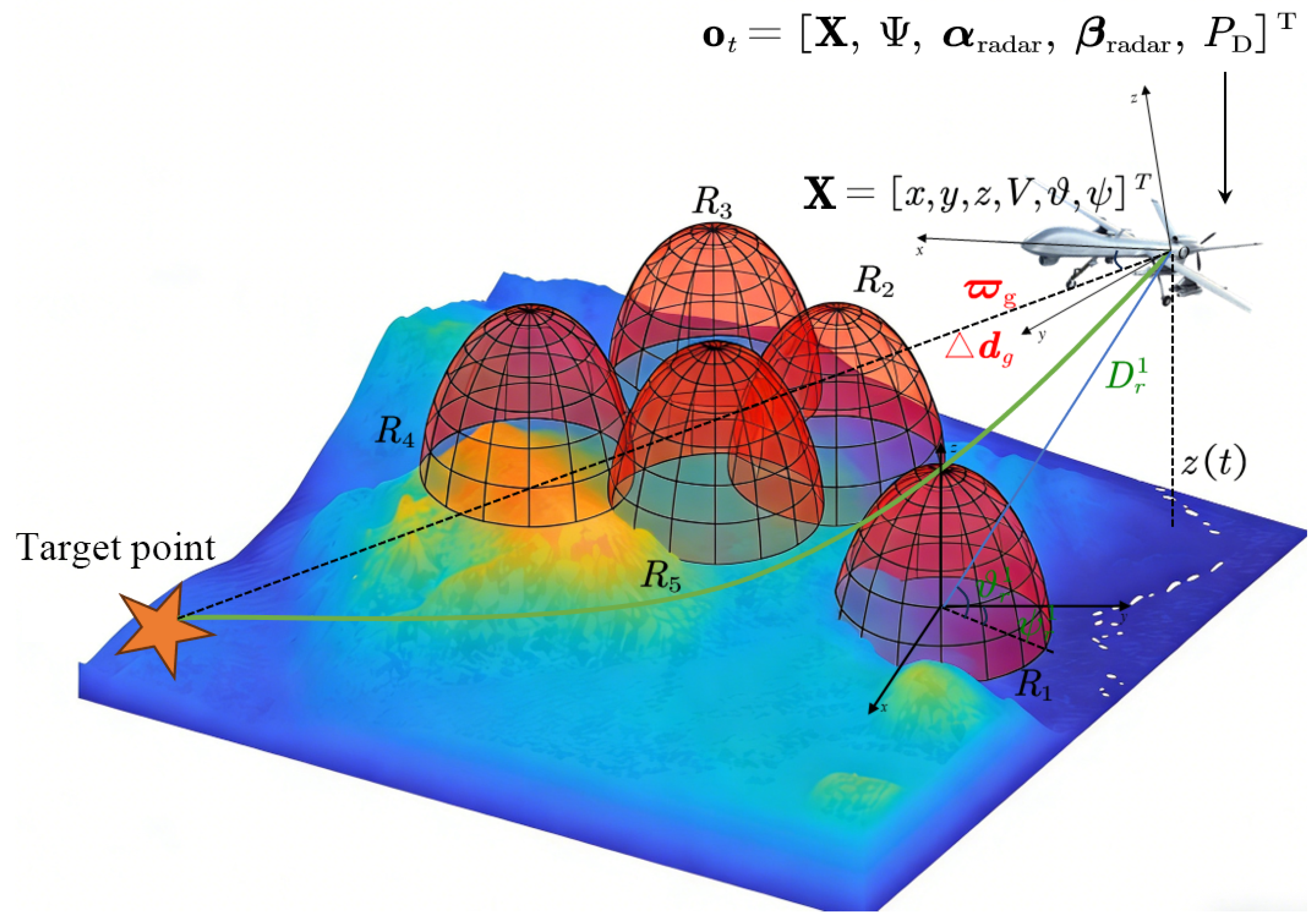
All components in Equation (25) are evaluated at time t. In implementation, the observation vector uses five radar slots. For scenarios with fewer than five active radars, inactive slots are filled with neutral placeholder values and excluded from the radar-risk calculation. This keeps the neural-network input dimension fixed across the two-radar and five-radar cases. A schematic illustration of the observation design for the UAV penetration mission under the POMDP framework is shown in Figure 5.

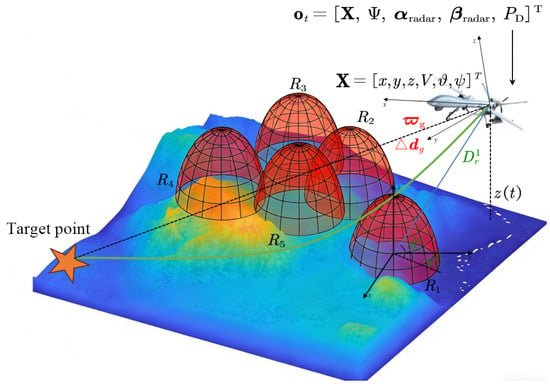
Figure 5. Observation–state design for UAV penetration path planning. The red domes represent radar coverage regions, while the colored surface depicts the terrain environment. The actor receives ${\mathbf{o}}_t$ in Equation (25); during training, each critic receives $({\mathbf{o}}_t,a_t)$. The radar-direction angles and $P_{\mathrm{D}}$ are computed by the simulation environment and included in ${\mathbf{o}}_t$.

3.2.2. Action Space

To ensure consistency between reinforcement learning training and the fixed-wing UAV dynamics model, the action space is defined as the control input of the fixed-wing UAV dynamics model. Given the explicit dynamic model, the UAV state can be updated through the control input, thereby driving state transitions in the environment.

$$\mathbf{A}=\left\{\begin{array}{c}{N}_x\in [-N_x^{\max },N_x^{\max }],\hfill \\ \Delta N_z\in [-\Delta N_z^{\max },\Delta N_z^{\max }],\hfill \\ \phi \in [-{\phi }^{\max },{\phi }^{\max }].\hfill \end{array}\right.$$

(26)

At decision step t, the SAC policy outputs the high-level planning action $a_t\in \mathbf{A}$. As defined in Equation (26), the three components of $a_t$ are $N_{x,t}$, $\Delta N_{z,t}$, and ${\phi }_t$, which denote the tangential-load-factor command, incremental normal-load-factor command, and roll-angle command, respectively. To ensure that the planned path satisfies the dynamic constraints of the fixed-wing UAV, the action magnitudes are bounded within the safe flight envelope. In this way, the output of the reinforcement learning agent remains dynamically feasible. By continuously adjusting these control commands, the agent not only determines the geometric flight path but also indirectly influences the electromagnetic characteristics of the UAV through attitude variations, thereby achieving coordinated optimization of penetration-time performance and modeled radar exposure.

3.2.3. Dynamic-RCS-Based Reward Function

The reward function guides the fixed-wing UAV to gradually learn effective decision-making policies based on perceived environmental information. In many reinforcement learning problems, sparse reward functions are adopted, such that rewards are obtained only when the task is completed. For the fixed-wing UAV penetration mission, the scarcity of feasible solutions and the low probability of successful task completion may lead to slow algorithmic convergence. A dense reward is therefore used to provide feedback at each state-transition step [29]. The distance-related feedback is computed from the current target distance and the clipped distance reduction between consecutive steps. The overall reward function can be expressed as follows:

$$\mathcal{R}={\mathcal{R}}_{\mathrm{target}}+{\mathcal{R}}_{\mathrm{radar}}+{\mathcal{R}}_{\mathrm{obs}}+{\mathcal{R}}_{\mathrm{arrive}}.$$

(27)

The target-distance and progress terms encourage penetration-time efficiency; the terrain-collision term represents flight safety; the radar term penalizes modeled exposure; and the arrival term encodes successful task completion.

(a) Target—Approaching Reward

To address the sparse-reward problem, a dense distance-based training reward is used. Since the flight speed of the fixed-wing UAV remains nearly constant during penetration, the mission time is approximately proportional to the path length. The distance-based reward is designed to encourage the fixed-wing UAV to approach the target more rapidly and is defined as follows:

$$\begin{array}{c}\hfill {\mathcal{R}}_{\mathrm{target}}={\gamma }_{\mathrm{dis}1}\left(-d_t\right)+{\gamma }_{\mathrm{dis}2}\mathrm{clip}\left(d_{t-1}-d_t,-1,1\right),\end{array}$$

(28)

where $d_t$ denotes the Euclidean distance between the UAV and the target point at the current time step, and $d_{t-1}-d_t$ represents the change in target distance between two consecutive time steps. ${\gamma }_{\mathrm{dis}1}$ and ${\gamma }_{\mathrm{dis}2}$ are weighting coefficients for the absolute-distance term and the progress term, respectively. To suppress training instability caused by excessively large reward magnitudes, the progress term is clipped using the clipping function $\mathrm{clip}(·,-1,1)$, which truncates its input to the interval $[-1,1]$. This design encourages the agent to learn an effective policy that continuously approaches the target, rather than pursuing unrealistic one-step gains. The resulting scalar reward is supplied directly to the SAC learner without further normalization.

(b) Radar detection penalty

As indicated by (3), radar detection probability is used as the surrogate for modeled radar-exposure risk. The detection probability of the j-th radar is denoted by $P_{d,j}$. Accordingly, the radar detection penalty is designed as follows:

$${\mathcal{R}}_{\mathrm{radar}}=-w_{\det }{P}_D=-w_{\det }\left(1-{\displaystyle \prod _{j=1}^m}\left(1-P_{\mathrm{d},j}\right)\right),$$

(29)

where $w_{\det }>0$ is the weighting factor for the radar-detection penalty.

(c) Fixed-wing UAV damage penalty

When the safety envelope of the fixed-wing UAV overlaps with the terrain, the UAV is considered to have collided with the terrain. In this case, a collision penalty is imposed, and the current episode is terminated. The penalty is defined as follows:

$${\mathcal{R}}_{\mathrm{obstacle}}=\left\{\begin{array}{cc}{P}_{col},\hfill & \mathrm{if}{r}_{\mathrm{uo}}<d_{\min };\hfill \\ 0,\hfill & \mathrm{otherwise},\hfill \end{array}\right.$$

(30)

where $r_{\mathrm{uo}}$ is the distance between the fixed-wing UAV and the terrain obstacle, $d_{\min }$ is the radius of the UAV safety envelope, and $P_{\mathrm{col}}<0$ is a preset collision penalty constant.

(d) Task completion reward

When the fixed-wing UAV reaches the target point, the terminal reward is defined as follows:

$${\mathcal{R}}_{\mathrm{arrive}}=\left\{\begin{array}{cc}{P}_{\mathrm{success}}+P_{\mathrm{step}},\hfill & \mathrm{if}{d}_t<d_{\mathrm{thres}};\hfill \\ 0,\hfill & \mathrm{otherwise},\hfill \end{array}\right.$$

(31)

where $d_t$ is the Euclidean distance between the fixed-wing UAV and the target point, $d_{\mathrm{thres}}$ denotes the target-reaching distance threshold, $P_{\mathrm{success}}>0$ is a preset terminal reward constant assigned when the UAV successfully reaches the target region, and $P_{\mathrm{step}}<0$ is a fixed negative reward term applied once upon successful target arrival.

At each state transition, the four components above are summed to form the scalar reward used for SAC training. No additional normalization is applied to this scalar reward. The clipping operation in Equation (28) applies only to the incremental-progress term, while all other terms retain the magnitudes set by their coefficients. The pseudocode for using the SAC algorithm in path search for fixed-wing UAVs is shown as Algorithm 1.

Algorithm 1: Dynamic RCS-Based SAC Path Planning

Input     : Battlefield environment, fixed-wing UAV dynamics model, dynamic RCS model, initial and terminal states;    Output  : planned path;   1: Initialization:   2: Initialize the policy network ${\pi }_{\theta }(a\left|o\right)$, two $\mathcal{Q}$-networks ${\mathcal{Q}}_{{\varphi }_1}(o,a)$ and ${\mathcal{Q}}_{{\varphi }_2}(o,a)$;   3: Initialize the target $\mathcal{Q}$-networks ${\mathcal{Q}}_{{\overline{\varphi }}_1}(o,a)$ and ${\mathcal{Q}}_{{\overline{\varphi }}_2}(o,a)$;   4: Initialize the target entropy ${\mathcal{H}}_{\mathrm{target}}=-\dim \left(\mathcal{A}\right)$, the temperature parameter $\kappa$, the replay buffer $\mathcal{D}$, and other parameters;   5: Training:   6: for each episode $e\in \{1,2,3,\dots \}$ do$\phantom{(}$   7:   Initialize the agent state and the training environment and obtain the initial observation $o_0$;   8:   for $t=0$ to $T_{\max }-1$ do   9:      Sample action $a_t$ from the current policy ${\pi }_{\theta }(·\mid o_t)$ 10:      Execute action $a_t$ and obtain the next observation $o_{t+1}$ 11:      Determine ${\delta }_t^{\mathrm{term}}$ from the resulting state: set it to 1 if terrain collision or target arrival occurs, and to 0 otherwise 12:      Evaluate ${\mathcal{R}}_{\mathrm{target}}$, ${\mathcal{R}}_{\mathrm{radar}}$, ${\mathcal{R}}_{\mathrm{obstacle}}$, and  ${\mathcal{R}}_{\mathrm{arrive}}$ for this transition using (28), (29), (30), and (31), respectively 13:      Set $r_t={\mathcal{R}}_{\mathrm{target}}+{\mathcal{R}}_{\mathrm{radar}}+{\mathcal{R}}_{\mathrm{obstacle}}+{\mathcal{R}}_{\mathrm{arrive}}$ 14:      Store $(o_t,a_t,r_t,o_{t+1},{\delta }_t^{\mathrm{term}})$ in the replay buffer $\mathcal{D}$ 15:      if $r_{\mathit{uo}}<d_{\min }$ or $d_t<d_{\mathit{thres}}$ then$\phantom{(}$ 16:         break 17:      end 18:      Set $o_t\leftarrow o_{t+1}$ 19:   end 20:   Randomly sample a mini-batch $\mathcal{B}={\left\{(o_i,a_i,r_i,o_{i+1},{\delta }_i^{\mathrm{term}})\right\}}_{i=1}^N$ from the replay buffer $\mathcal{D}$; 21:   Sample the next action $a_{i+1}^{\prime }$ by (20) and compute the target value $y_i$ by (19) 22:   Update the $\mathcal{Q}$-network parameters by minimizing the critic loss $L_{\mathcal{Q}}\left({\varphi }_i\right)$, $i=1,2$ by (18); 23:   Update the policy network by minimizing the objective $L_{\pi }\left(\theta \right)$ by (21); 24:   Update the temperature parameter $\kappa$ by minimizing the loss $L\left(\kappa \right)$ by (22); 25: end 26: return the corresponding planned path for the fixed-wing UAV

4. Simulation Experiments and Semi-Physical Validation

4.1. Simulation Environment and Evaluation Metrics

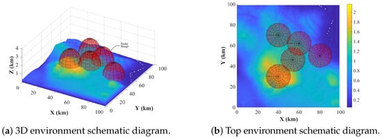
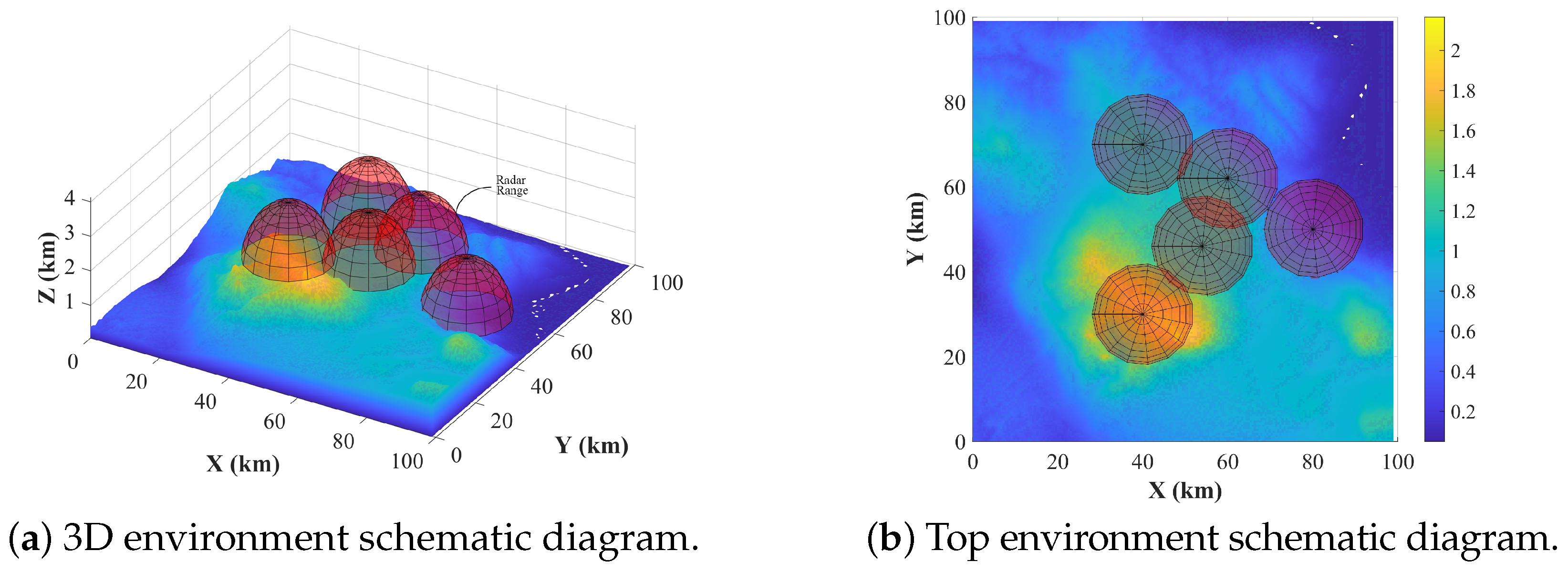
Simulation experiments are conducted in a randomly generated penetration mission environment. The environment size is $100\mathrm{km}\times 100\mathrm{km}\times 2\mathrm{km}$ along the x-, y-, and z-axes of the north-east-up coordinate system, respectively. An initial point and a target region are specified within the environment. Five radars are deployed around the nominal route connecting the initial point and the target region. For the stochastic scenario evaluation, the UAV initial position is fixed at the value listed in Table 1, while the three initial attitude components are sampled uniformly from $[-\pi /8,\pi /8]$. The terminal position and radar-center coordinates are sampled within the scenario-dependent bounds in Table 1. The radar detection radius remains $12\mathrm{km}$; consequently, the detection regions vary spatially with the sampled radar-center locations. Figure 6 illustrates one representative mission instance.

Table 1. Sampling specifications for the stochastic scenario evaluation (unit: km).

Scenario	Radar Position Distribution	UAV Initial and Target Position Distribution
Scenario 1	$x_{\mathrm{r}1}\in [38,42]$, $y_{\mathrm{r}1}\in [68,72]$, $z_{\mathrm{r}1}=z_1$	Initial position: $(10,10,0.83)$; target position distribution: $x\in [88,92]$, $y\in [88,92]$, and $z\in [1.40,1.44]$
	$x_{\mathrm{r}2}\in [58,62]$, $y_{\mathrm{r}2}\in [60,64]$, $z_{\mathrm{r}2}=z_2$
	$x_{\mathrm{r}3}\in [52,56]$, $y_{\mathrm{r}3}\in [44,48]$, $z_{\mathrm{r}3}=z_3$
	$x_{\mathrm{r}4}\in [38,42]$, $y_{\mathrm{r}4}\in [28,32]$, $z_{\mathrm{r}4}=z_4$
	$x_{\mathrm{r}5}\in [78,82]$, $y_{\mathrm{r}5}\in [48,52]$, $z_{\mathrm{r}5}=z_5$
Scenario 2	$x_{\mathrm{r}1}\in [38,42]$, $y_{\mathrm{r}1}\in [68,72]$, $z_{\mathrm{r}1}=z_1$	Initial position: $(10,10,0.83)$
	$x_{\mathrm{r}2}\in [53,57]$, $y_{\mathrm{r}2}\in [43,47]$, $z_{\mathrm{r}2}=z_2$	Target position distribution: $x\in [88,92]$, $y\in [88,92]$, and $z\in [1.40,1.44]$

Figure 6. Schematic diagram of the simulation environment.

The simulation environment internally maintains the true state ${\mathbf{s}}_t$ for state transition, termination judgment, and reward computation. During both training and evaluation, the agent receives only the observation ${\mathbf{o}}_t$ as the policy input, without explicit access to the exact radar locations or radar parameters. Specifically, the observation ${\mathbf{o}}_t$ includes the UAV’s own state and task-oriented state information. The radar-direction angles and the aggregate modeled radar-detection probability are computed internally by the simulation environment and are also included in ${\mathbf{o}}_t$, as defined in Equation (25).

A multilayer perceptron (MLP) with ReLU activation functions is adopted as the neural network architecture. The actor and each of the two critic networks use five fully connected hidden layers with 128 units per layer. The planned path is represented by a sparse waypoint sequence. Within one complete planning process, the SAC policy generates one high-level action at each decision step. This action is applied over a $20\mathrm{s}$ interval of simulated flight time. The fixed-wing model then generates the state at the end of this interval, from which the next observation and waypoint are obtained. Given the adopted flight-speed range of 30–$40\mathrm{m}/\mathrm{s}$, each $20\mathrm{s}$ interval corresponds to approximately $600–800\mathrm{m}$ of traveled distance between successive sparse waypoint samples. Accordingly, $20\mathrm{s}$ is the waypoint or decision interval rather than the frequency of complete-path planning. During SAC training, the simulation environment updates the UAV state and simulated situation at $1000\mathrm{Hz}$, corresponding to a numerical simulation time step of $\Delta t=0.001\mathrm{s}$.

To avoid excessive ineffective decisions that could slow convergence during training, the maximum episode length is set to 3000 decision steps. Each episode terminates when one of the following conditions is satisfied: the maximum episode length is reached, the fixed-wing UAV collides with the terrain, or it reaches the target. For the subsequent mission-level comparison over the 100 stochastic scenarios, the retained policy was trained for $5.0\times {10}^5$ environment-interaction steps using seed 123. Separately, for the multi-seed training analysis, SAC was trained independently in 100 runs, each initialized with a distinct random seed and trained for $1.0\times {10}^6$ environment-interaction steps. The former evaluates the mission-level performance of a fixed policy across stochastic scenarios, whereas the latter assesses the robustness and reproducibility of SAC training across distinct random seeds. The algorithm hyperparameters, simulation-environment settings, and fixed-wing UAV performance constraints are listed in Table 2 and Table 3.

Table 2. Environment and algorithm parameter settings.

Variable	Value	Variable	Value
$C_d$	$-0.1 {\mathrm{m}}^2{\mathrm{km}}^{-4}$	${\gamma }_{di{s}_1}$	1
${\gamma }_{di{s}_2}$	1	$w_{\det }$	200
$R_{\det }$	12 km	$d_{\min }$	0.1 km
g	9.81	learning_rate	0.000125
batch_size	64	$\gamma$	0.99
$\tau$	0.005	learning_starts	10,000
buffer_size	100,000	$\kappa$	0.1
$P_{\mathrm{col}}$	$-50$	$P_{\mathrm{success}}$	50
$P_{\mathrm{step}}$	$-0.3$	$d_{\mathrm{thres}}$	$3\mathrm{km}$

Table 3. Vehicle constraints.

Variable	Range/Value	Variable	Range/Value
V	$[30,40]$ m/s	$\vartheta$	$[-0.5,0.5]\mathrm{rad}$
$N_x$	$[-0.2,0.2]$	$\Delta N_z$	$[-0.2,0.2]$
$\phi$	$[-0.1,0.1]\mathrm{rad}$	$R_{\mathrm{safe}}$	100 m

The evaluation considers both penetration time and modeled radar-exposure risk. Accordingly, four metrics are used to assess the simulation results:

(1) Penetration time $t_{\mathrm{p}}$

During penetration, the UAV spends most of the mission in cruise flight; therefore, the path length largely determines the penetration time. Therefore, the penetration time should be minimized so that the UAV can traverse the threat region quickly and reduce the risk of radar detection. It is defined as $t_{\mathrm{p}}=t_{\mathrm{f}}-t_0$.

(2) Average radar detection probability $P_{\mathrm{D}}^{\mathrm{avg}}$

During penetration, the radar detection probability reflects the UAV’s exposure risk. A lower value indicates lower modeled exposure to radar detection and tracking. It is defined as follows:

$$P_{\mathrm{D}}^{\mathrm{avg}}={\displaystyle \frac{1}{t_{\mathrm{p}}}}{\int }_{t_0}^{t_{\mathrm{f}}}{P}_{\mathrm{D}}\left(t\right)dt.$$

(32)

(3) Average radar cross-section ${\sigma }^{\mathrm{avg}}$

Because radar-cross-section anisotropy must be considered during penetration, the average radar cross-section is used to quantify the extent to which the UAV reduces its RCS by adjusting its relative state with respect to the radar. Because the RCS directly affects detection risk only when the UAV is within the radar coverage region, the averaging interval is chosen as $[t_{\mathrm{in}},t_{\mathrm{out}}]$, and the metric is defined as follows:

$${\sigma }^{\mathrm{avg}}={\displaystyle \frac{1}{t_{\mathrm{r}}}}{\int }_{t_{\mathrm{in}}}^{t_{\mathrm{out}}}\sigma \left(t\right)dt,$$

(33)

where $t_{\mathrm{r}}=t_{\mathrm{out}}-t_{\mathrm{in}}$ denotes the duration for which the UAV is exposed to the radar-threat region.

(4) Algorithm computation time $t_{\mathrm{a}}$

For each evaluation trial, $t_{\mathrm{a}}$ denotes the computation time required by the algorithm to complete one path-planning run.

4.2. Numerical Simulation Results and Comparative Analysis

4.2.1. Path-Planning Performance in Randomized Scenarios

The mission-level evaluation comprised 100 independently generated stochastic scenarios within the $100\mathrm{km}\times 100\mathrm{km}$ mission area. In each scenario, the UAV boundary states and radar deployment were generated according to the sampling specifications in Table 1. All compared planning methods were evaluated using the same realization of each stochastic scenario, providing common terrain, threat, boundary, and mission conditions for comparison. To investigate algorithm performance under different threat scales, two representative radar-deployment scenarios are considered, namely, a two-radar scenario and a five-radar scenario. The two-radar and five-radar cases use separately trained policies with the same fixed observation structure and network architecture. The environmental parameter settings for each scenario are listed in Table 1. Here, $x_{\mathrm{r}i}$, $y_{\mathrm{r}i}$, and $z_{\mathrm{r}i}$ denote the position coordinates of the i-th radar, where $i=1,2,\dots ,N_{\mathrm{r}}$, and $N_{\mathrm{r}}=2$ or 5 corresponds to the two-radar scenario and the five-radar scenario, respectively. In addition, $z_i$ represents the terrain elevation corresponding to the planar position $(x_{\mathrm{r}i},y_{\mathrm{r}i})$ of the i-th radar. Based on the performance metrics defined in the previous subsection, the metrics are summarized separately for the successful trials of each method. For the planning method j, let ${\mathcal{S}}_j$ denote the set of stochastic scenario realizations in which the UAV successfully reaches the target, and let $M_{\mathrm{S},j}=\left|{\mathcal{S}}_j\right|$ denote the corresponding number of successful trials. The success-conditioned mean metrics are defined as follows:

$$\begin{array}{cc}\hfill \overline{t_{\mathrm{p},j}}& ={\displaystyle \frac{1}{M_{\mathrm{S},j}}}\sum _{m\in {\mathcal{S}}_j}{t}_{\mathrm{p},j,m},\overline{P_{\mathrm{D},j}^{\mathrm{avg}}}={\displaystyle \frac{1}{M_{\mathrm{S},j}}}\sum _{m\in {\mathcal{S}}_j}{P}_{\mathrm{D},j,m}^{\mathrm{avg}},\hfill \\ \hfill \overline{{\sigma }_j^{\mathrm{avg}}}& ={\displaystyle \frac{1}{M_{\mathrm{S},j}}}\sum _{m\in {\mathcal{S}}_j}{\sigma }_{j,m}^{\mathrm{avg}},\overline{t_{\mathrm{a},j}}={\displaystyle \frac{1}{M_{\mathrm{S},j}}}\sum _{m\in {\mathcal{S}}_j}{t}_{\mathrm{a},j,m}.\hfill \end{array}$$

(34)

Here, m identifies one stochastic scenario realization. Only the realizations belonging to ${\mathcal{S}}_j$ enter the averages in Equation (34). The total number of stochastic scenario realizations evaluated for each method remains $N=100$.

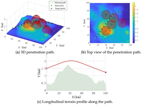
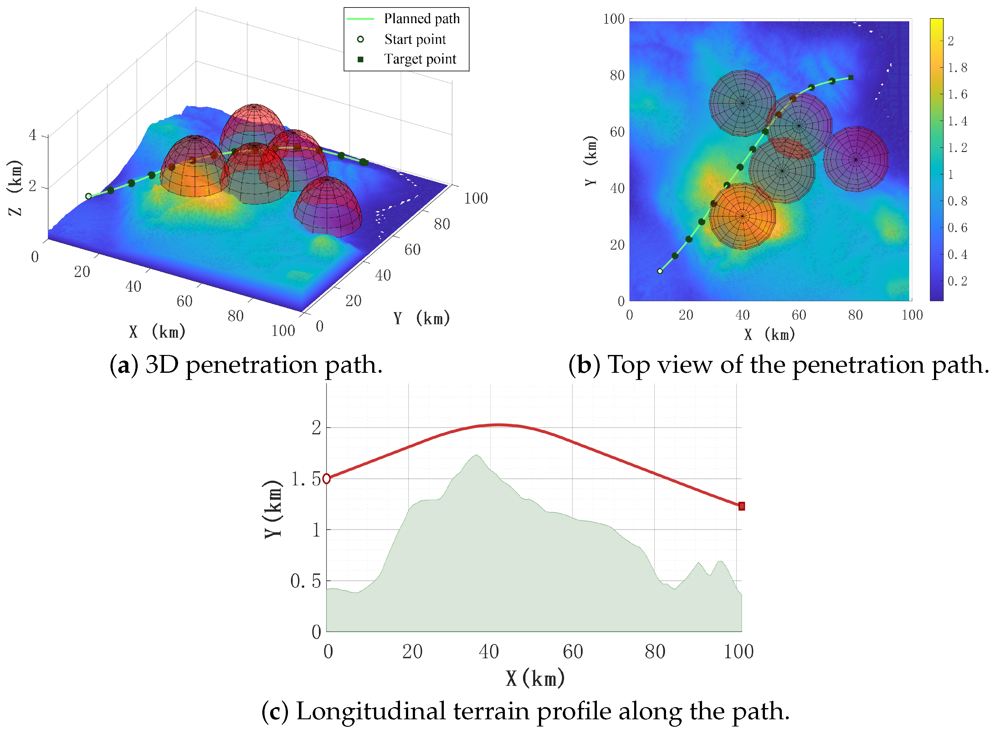
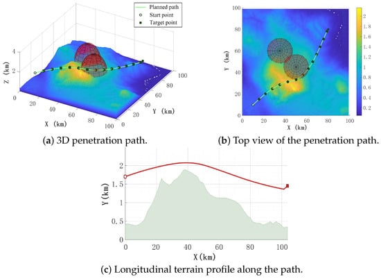
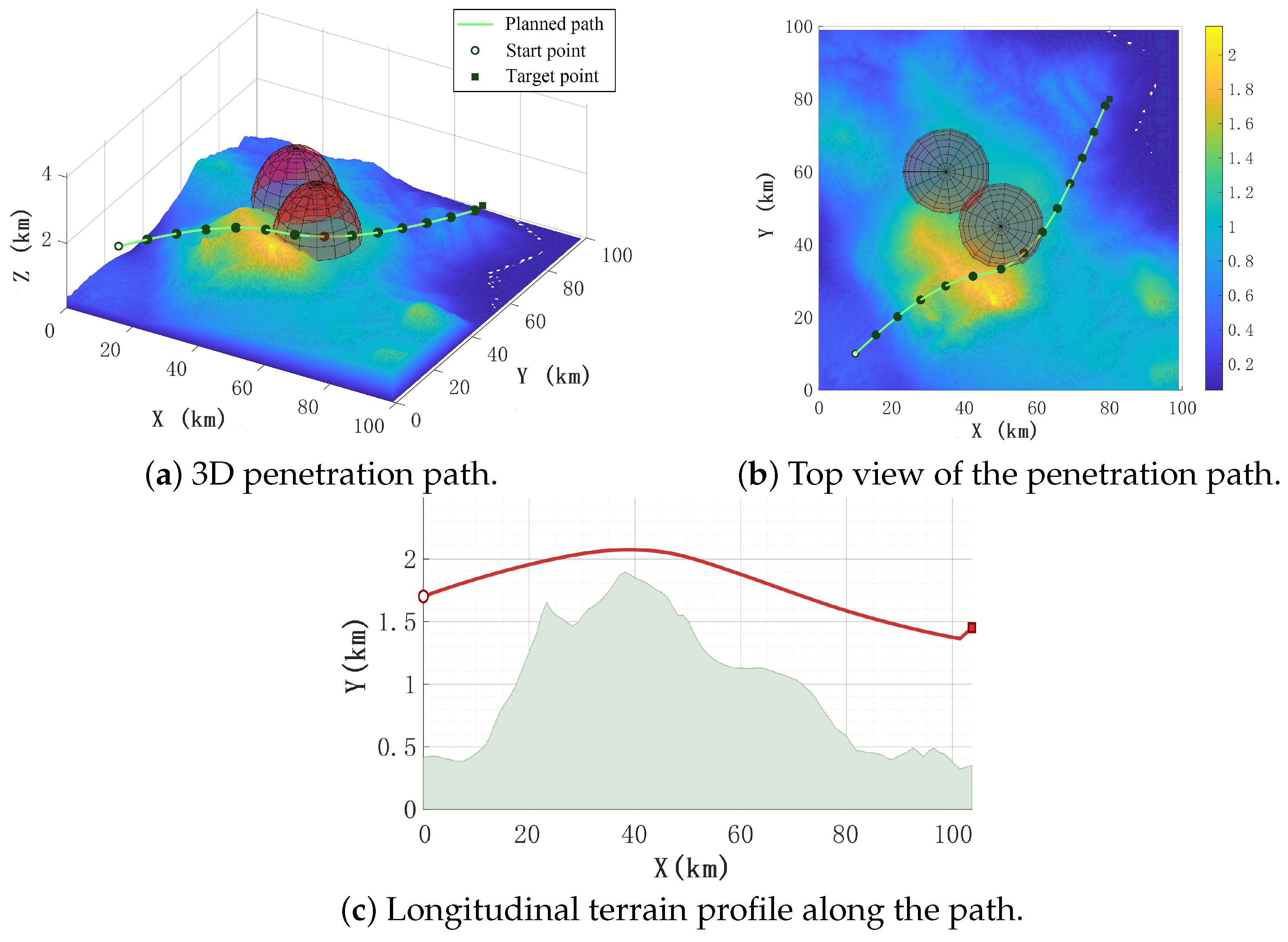
Figure 7 and Figure 8 present the path planning results of the UAV in Scenario 1 and Scenario 2, respectively, for representative realizations whose performance is close to the corresponding stochastic-scenario average. Scenario 1 corresponds to the five-radar case, whereas Scenario 2 corresponds to the two-radar case. The white dot denotes the starting point of the planned path, while the black square denotes the terminal point. To avoid overly dense path points that may affect visualization, a path marker is plotted every eight sampled points along the planned path sequence. It can be observed that the UAV effectively avoids the mountainous terrain while reducing the radar detection probability by passing through the edges of the radar coverage regions as much as possible. The following analysis mainly focuses on the simulation results of Scenario 1.

Figure 7. Path planning results of UAV penetration in Scenario 1.

Figure 8. Path planning results of UAV penetration in Scenario 2.

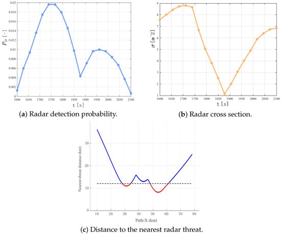
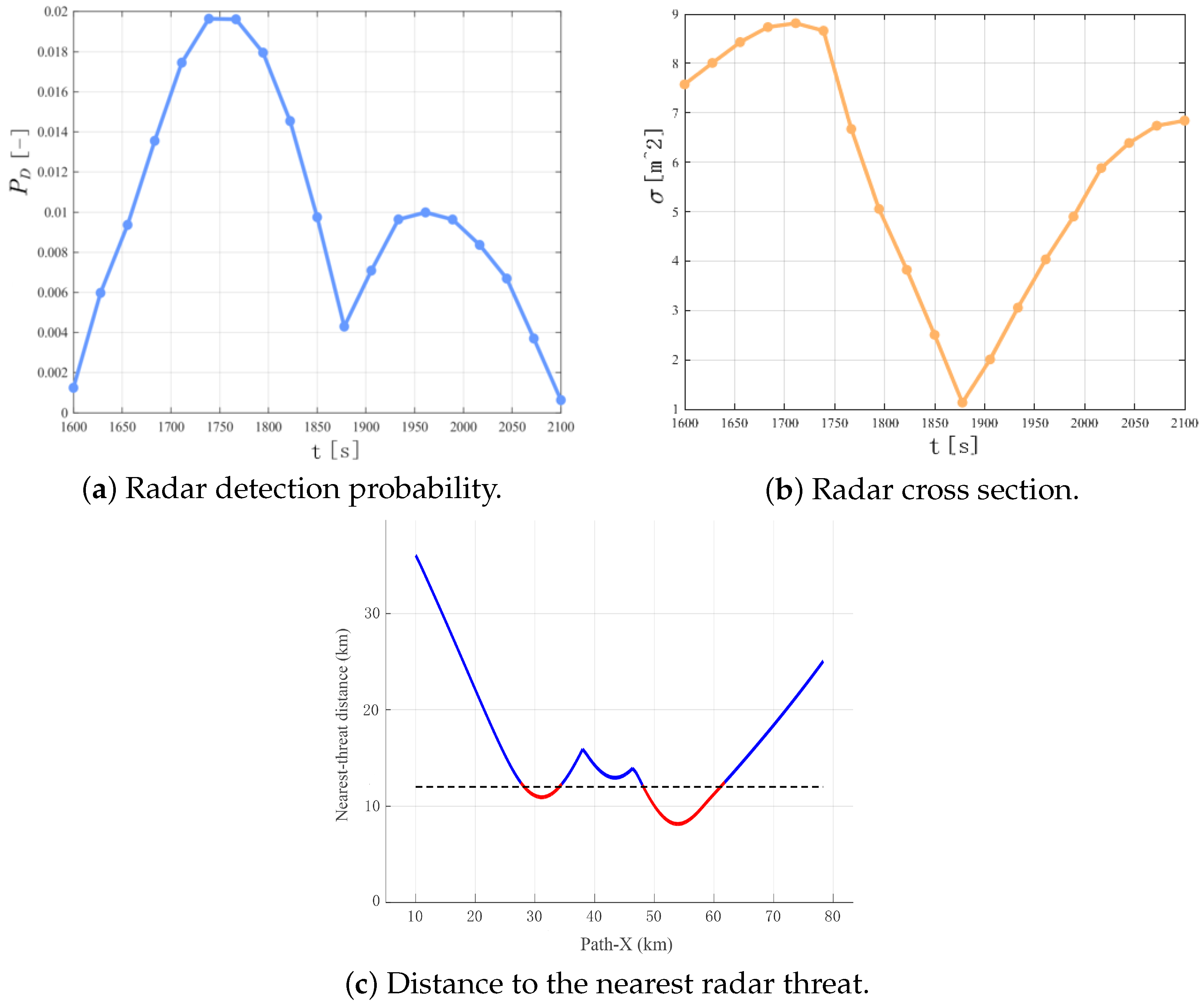
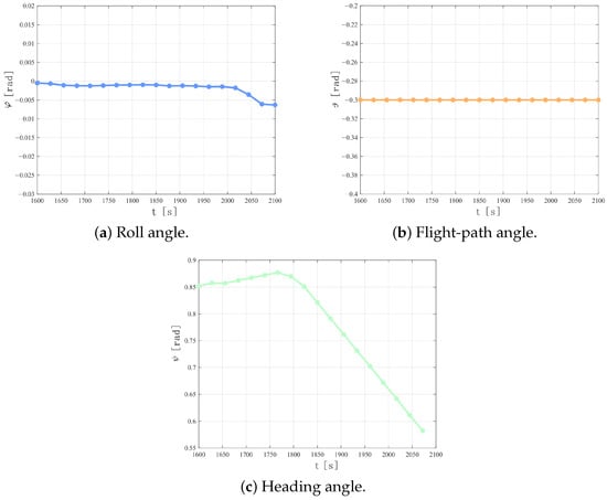
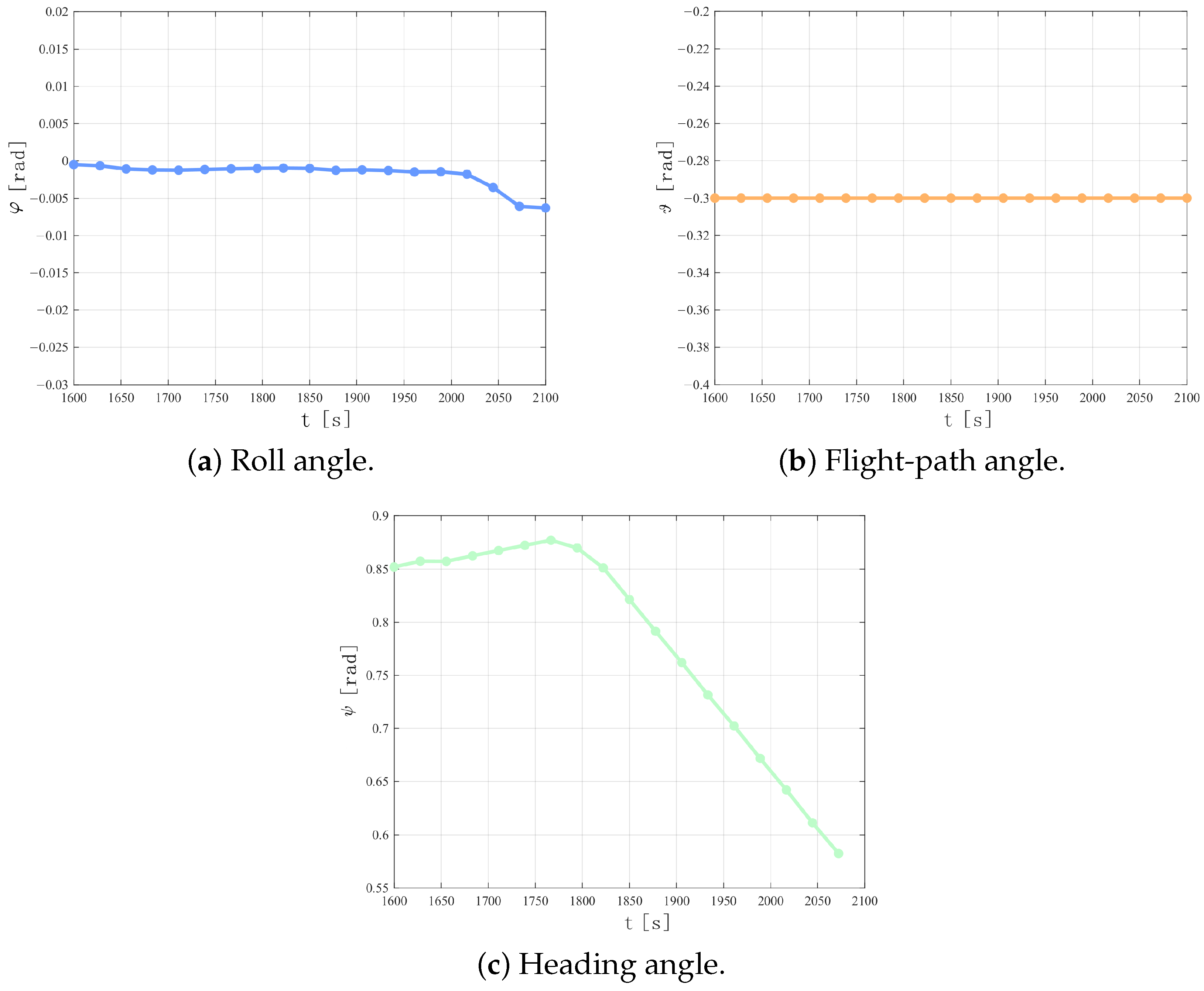
During the flight, the UAV enters the detection regions of Radar No. 2 and Radar No. 4; therefore, these radars contribute to its modeled exposure. Taking the radar-related variables of Radar No. 2 as an example, it can be observed from Figure 9 and Figure 10 that the UAV enters the radar-threat region at approximately $1600\mathrm{s}$. From $1600\mathrm{s}$ to $1750\mathrm{s}$, the radar detection probability continues to increase. Around $1750\mathrm{s}$, the UAV reduces its radar cross-section by adjusting its heading angle, thereby lowering the radar detection probability. After approximately $1875\mathrm{s}$, although the radar cross-section increases again, the Euclidean distance between the UAV and the radar becomes larger; therefore, the radar detection probability remains within a relatively low range.

Figure 9. Radar detection-related variables during UAV penetration.

Figure 10. UAV attitude variations during periods of high radar detection probability.

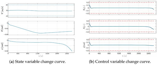
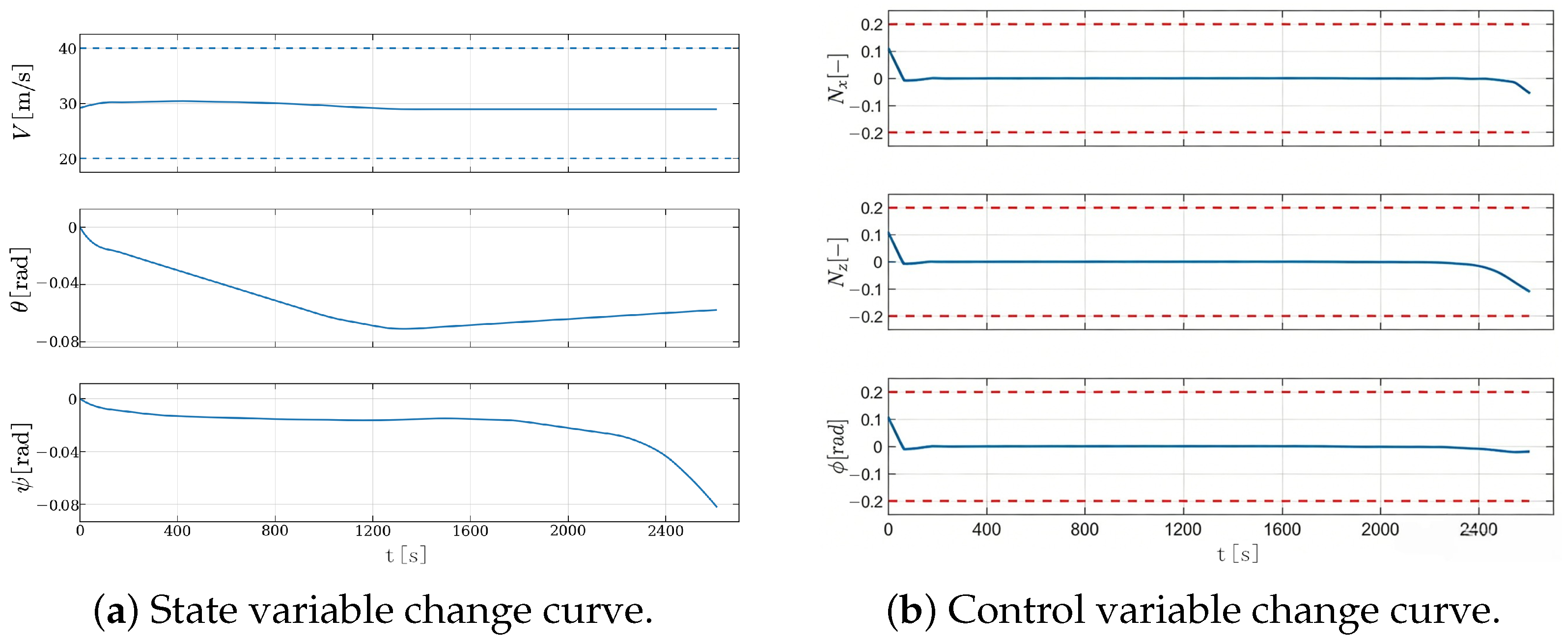
Furthermore, as shown in Figure 9c, the distance between the UAV and the nearest radar threat decreases to a relatively small value only during the short time interval when the UAV enters the detection region, and then rapidly increases again while remaining above the safe distance. Therefore, the proposed method effectively suppresses radar detection risk through a coordinated mechanism that reduces the radar cross-section while increasing the separation distance from the radar. In addition, Figure 11 presents the detailed state and control variables associated with the path planned by the proposed algorithm. All these variables satisfy the prescribed performance constraints of the UAV.

Figure 11. Time histories of UAV variables during flight in Scenario 1. The horizontal dashed lines indicate the prescribed upper and lower bounds of the corresponding variables.

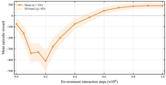
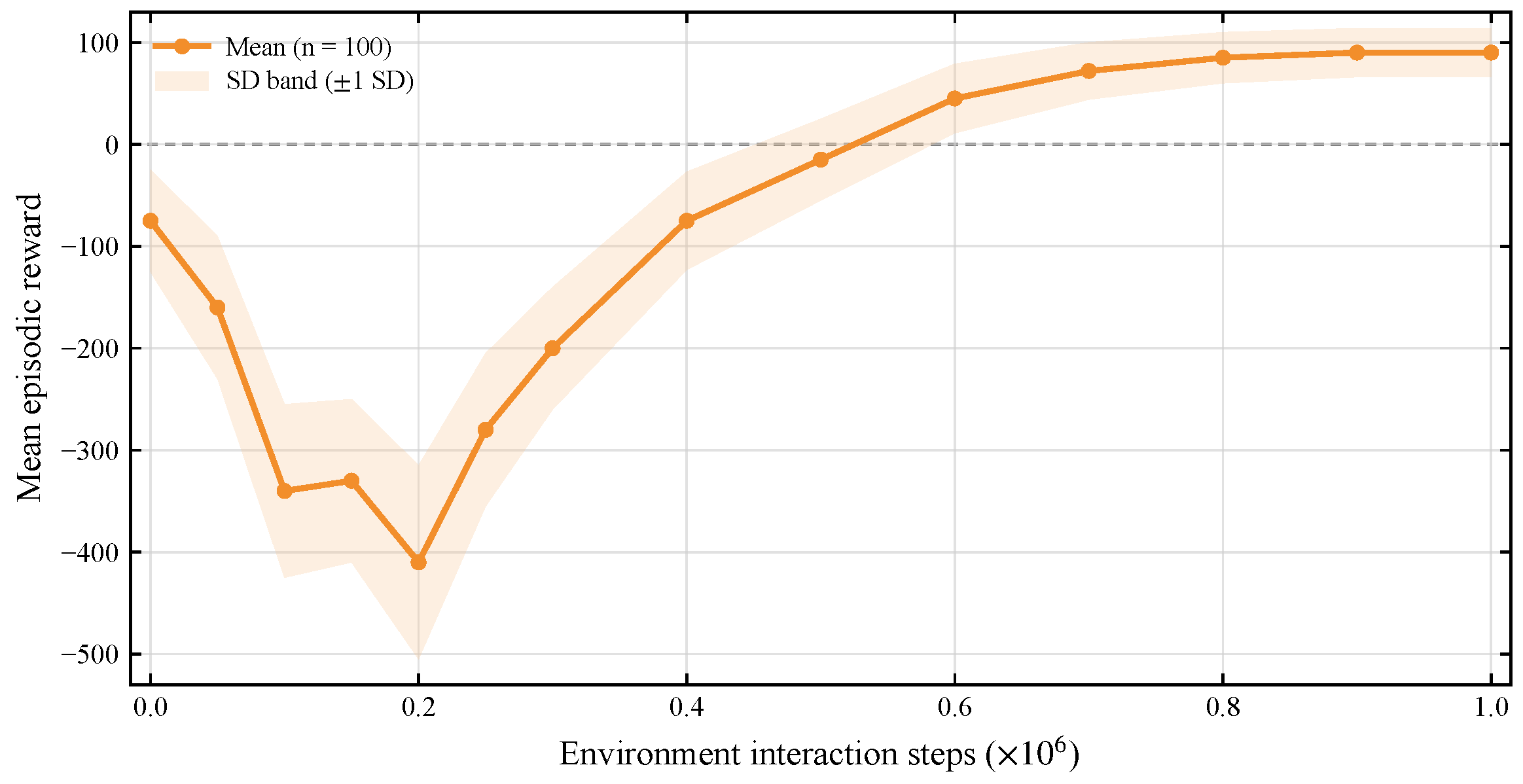
Figure 12 presents the mean episodic reward across 100 independently trained SAC runs initialized with distinct random seeds. The solid line denotes the across-seed mean, and the shaded band denotes $\pm 1$ standard deviation across seeds at matched environment-interaction steps. This analysis characterizes the learning trend and the variability caused by stochastic initialization and sampling, thereby assessing the robustness and reproducibility of the SAC training process. In contrast, the mission-level evaluation uses the policy trained for $5.0\times {10}^5$ environment-interaction steps using seed 123 and assesses its performance across 100 stochastic mission scenarios. The seed and training horizon for this policy were fixed before the mission-level evaluation and were not selected based on the multi-seed statistics in Figure 12 or downstream mission-level performance.

Figure 12. Mean episodic reward over $1.0\times {10}^6$ environment-interaction steps across 100 independent SAC training runs initialized with distinct random seeds. The solid line denotes the across-seed mean, and the shaded band denotes $\pm 1$ standard deviation at matched environment-interaction steps.

4.2.2. Comparative Analysis with Static RCS and Baseline Algorithms

To evaluate the impact of RCS dynamic characteristics on path planning, a control group experimental framework was established in this study. Referring to the criterion for maximizing the survival probability of fixed-wing UAV proposed in [19], the control group adopted a static RCS modeling method and set the RCS value as the maximum theoretical value achievable in the aircraft coordinate system. This design effectively separates the contribution of attitude stealth to optimization results by eliminating the RCS dynamic adjustment mechanism. The dynamic- and maximum-static-RCS configurations were evaluated under the same scenario conditions, including identical terrain, radar deployment, initial state, target state, and termination criteria.

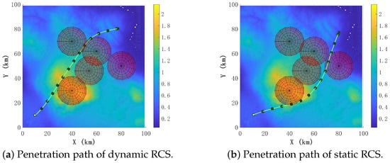
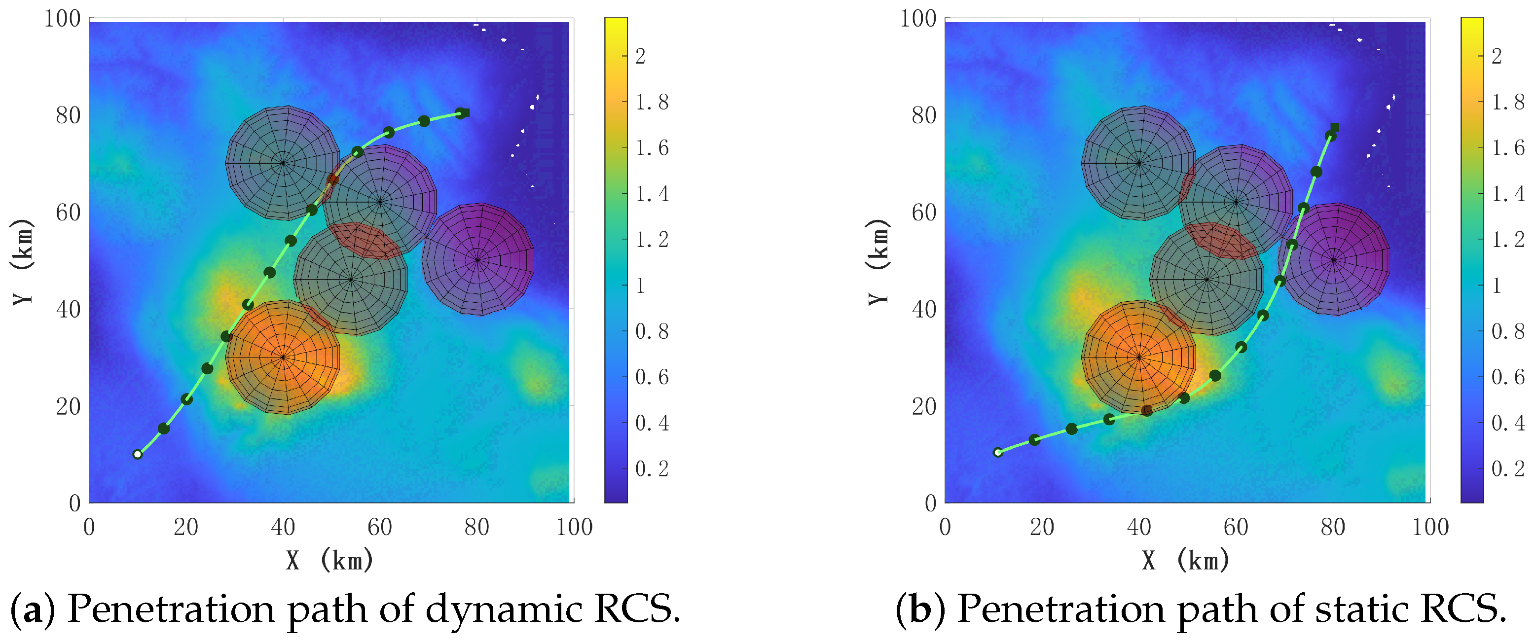
As shown in Figure 13, it can be seen that two different flight paths were selected for both dynamic RCS and static RCS models. Among them, the static RCS model uses the maximum theoretical value of RCS as a reference, so the planned path is more conservative and prioritizes avoiding the radar detection range, resulting in a relatively long flight time. The dynamic RCS model fully considers the relative position changes between the target and the radar during the flight process, accounts for the relative-position and attitude variations along the planned path, and effectively reduces the RCS value in the radar direction, allowing it to select a path with a shorter mission time while meeting the requirements for penetration.

Figure 13. Penetration-path comparison between the dynamic-RCS configuration and the maximum-static-RCS stress-test configuration.

The mean metrics in Table 4 were calculated using the same number of successful trials for the dynamic- and maximum-static-RCS configurations.

Table 4. Comparison of evaluation indicators between the proposed algorithm and static RCS model. Values are reported as mean ± standard deviation.

Evaluation Indicators	Dynamic RCS	Static RCS
$t_{\mathrm{p}}\left(\mathrm{s}\right)$	$2706.5\pm 227.3$	$2890.58\pm 285.0$
$P_{\mathrm{D}}^{\mathrm{avg}}$	$0.0497\pm 0.0072$	$0.0530\pm 0.0078$
${\sigma }^{\mathrm{avg}}\left({\mathrm{m}}^2\right)$	$6.6649\pm 0.612$	$12.00\pm 0.00$
$t_{\mathrm{a}}\left(\mathrm{s}\right)$	$2.849\pm 0.213$	$2.549\pm 0.235$

Under the adopted maximum-static-RCS assumption, the static-RCS configuration gives longer mean penetration time, higher modeled detection probability, and higher mean RCS than the dynamic-RCS configuration. Because the fixed-RCS value is set to the theoretical maximum, this comparison is interpreted as a conservative stress test rather than as a neutral comparison with nominal or mean static-RCS assumptions. Accordingly, the results demonstrate the observed effect of the adopted maximum-static-RCS assumption within the present planning framework. Comparisons with nominal or mean static RCS values, as well as broader fixed-RCS ablations, were not conducted and remain future work.

All compared methods were evaluated using the same 100 stochastic scenario realizations and common terrain, radar threats, boundary conditions, termination criteria, metrics, hardware, and fixed-wing feasibility assessment. Among these realizations, SAC, A*, the pseudo-spectral method, and PPO successfully reached the target in 93, 88, 85, and 89 trials, respectively. Table 5 reports the mean ± standard deviation of performance metrics for the successful trials for each method. Collision and timeout trials are excluded from these metric summaries and are reported separately as terminal outcomes in Table 6.

Table 5. Performance metrics among successful trials in the 100 shared stochastic scenarios. Values are reported as mean ± standard deviation.

Algorithm	${\mathit{t}}_{\mathbf{p}}\left(\mathbf{s}\right)$	${\mathit{P}}_{\mathbf{D}}^{\mathbf{avg}}$	${\mathit{\sigma }}^{\mathbf{avg}}\left({\mathbf{m}}^2\right)$	${\mathit{t}}_{\mathbf{a}}\left(\mathbf{s}\right)$
Proposed Algorithm ($n=93$)	$2706.5\pm 227.3$	$0.0497\pm 0.0072$	$6.6649\pm 0.612$	$2.849\pm 0.213$
A* ($n=88$)	$3352.04\pm 412.6$	$0.0523\pm 0.0081$	$8.6327\pm 0.985$	$10.079\pm 2.674$
Pseudo-spectral method ($n=85$)	$2789.06\pm 203.5$	$0.0464\pm 0.0065$	$6.3523\pm 0.548$	$15.235\pm 4.128$
PPO ($n=89$)	$3273.48\pm 438.7$	$0.0472\pm 0.0078$	$6.5235\pm 0.591$	$2.594\pm 0.187$

Table 6. Mission outcomes over the 100 shared stochastic scenarios.

Algorithm	Success, n (%)	Collision, n (%)	Timeout, n (%)
Proposed Algorithm (SAC)	93 (93.0%)	4 (4.0%)	3 (3.0%)
A*	88 (88.0%)	0 (0.0%)	12 (12.0%)
Pseudo-spectral method	85 (85.0%)	2 (2.0%)	13 (13.0%)
PPO	89 (89.0%)	6 (6.0%)	5 (5.0%)

Each stochastic scenario was assigned one mutually exclusive terminal outcome. A timeout denotes that the maximum episode length of 3000 decision steps was reached without either successful target arrival or terrain collision.

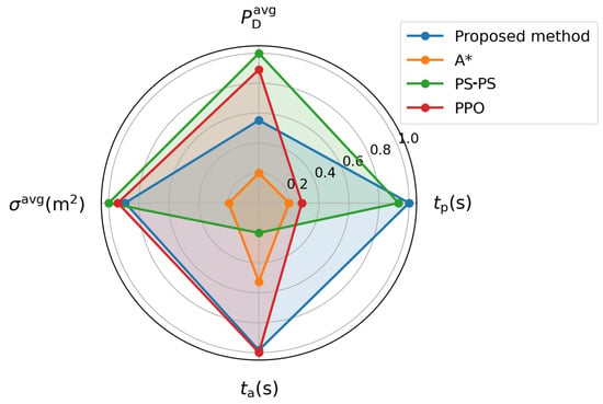
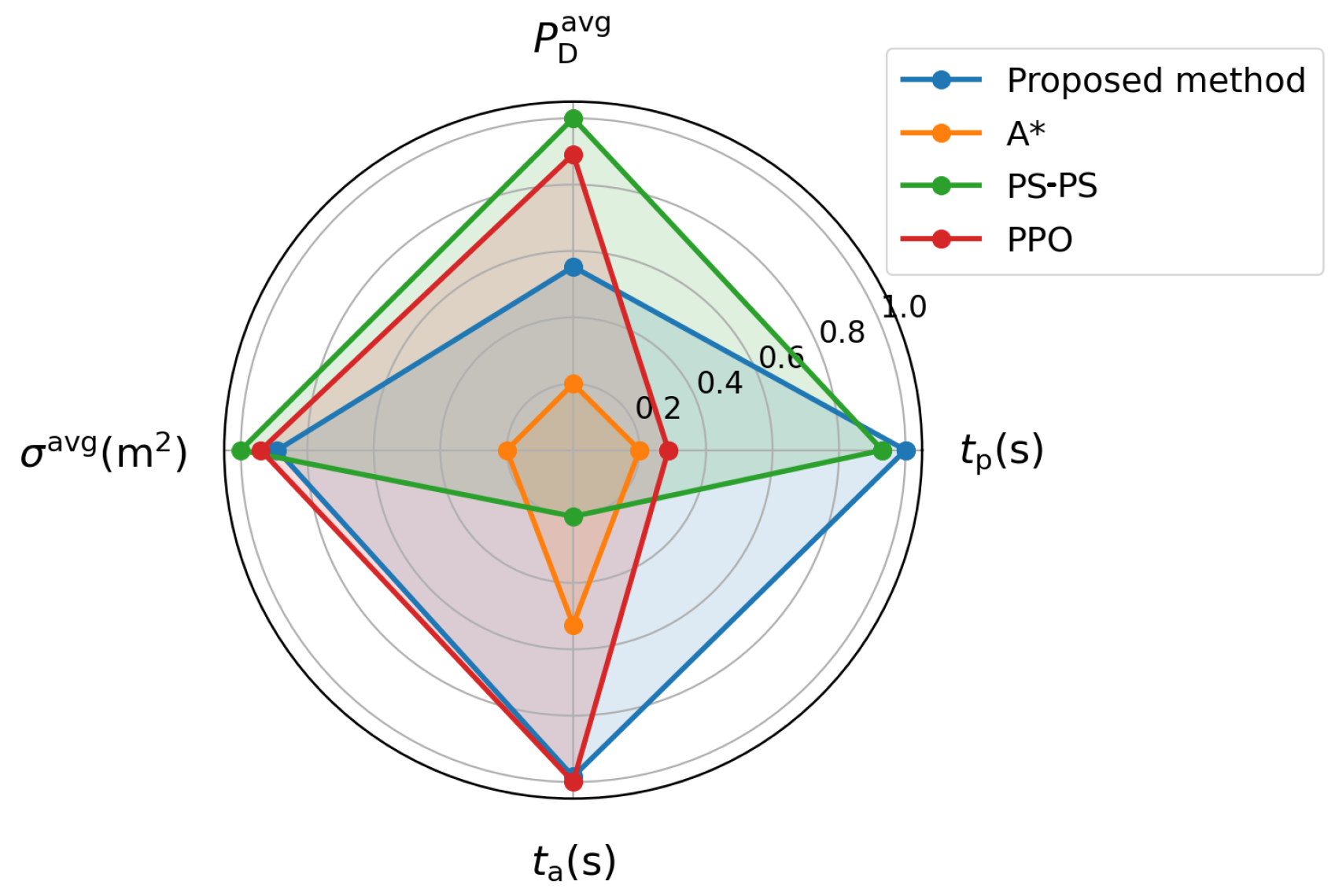
Among the successful trials of each method, SAC gives the shortest mean penetration time, reducing it by 19.26%, 2.96%, and 17.32% relative to A*, the pseudo-spectral method, and PPO, respectively. Among these successful trials, its mean detection probability and mean RCS are lower than those of A* but higher than those of the pseudo-spectral method and PPO. Among successful trials, the mean computation time for one complete SAC path-planning run is 2.849 s, below that of A* (10.079 s) and the pseudo-spectral method (15.235 s), but above that of PPO (2.594 s). The results therefore show a time–exposure–computation trade-off under one weighting configuration, not overall dominance. The comparative results are shown in Figure 14. For visualization only, each metric in Table 5 is first transformed into an inverse min–max normalized benefit score,

$$b_{ij}={\displaystyle \frac{{\max }_m{q}_{mj}-q_{ij}}{{\max }_m{q}_{mj}-{\min }_m{q}_{mj}}},$$

(35)

where $q_{ij}$ is the raw value of metric j for method i. A larger $b_{ij}$ indicates better performance for that individual metric. In Figure 14, $b_{ij}$ is displayed using the radial mapping ${\rho }_{ij}=0.2+0.8b_{ij}$ for readability; this plotting-only scaling does not change the relative ranking. The enclosed radar-chart area is not interpreted as an overall performance score.

Figure 14. Normalized radar-chart comparison of the planning methods. The inverse min–max normalized benefit scores are calculated from the raw values in Table 5 (successful trials only) and displayed using the radial mapping ${\rho }_{ij}=0.2+0.8b_{ij}$ for readability. A larger radial value indicates a lower raw detection probability, penetration time, planning time, or RCS. The enclosed area is not interpreted as an overall performance score.

4.3. Semi-Physical Hardware-in-the-Loop Validation

The semi-physical hardware-in-the-loop (HIL) evaluation was conducted using two representative mission configurations also considered in the numerical experiments: Scenario 1 with five modeled radar regions and Scenario 2 with two modeled radar regions. The HIL evaluation examines onboard path planning, waypoint transfer, PX4 closed-loop tracking, and software–hardware communication.

4.3.1. HIL Platform and Workflow

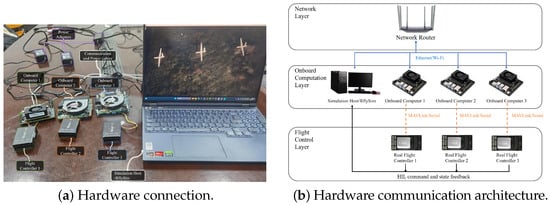
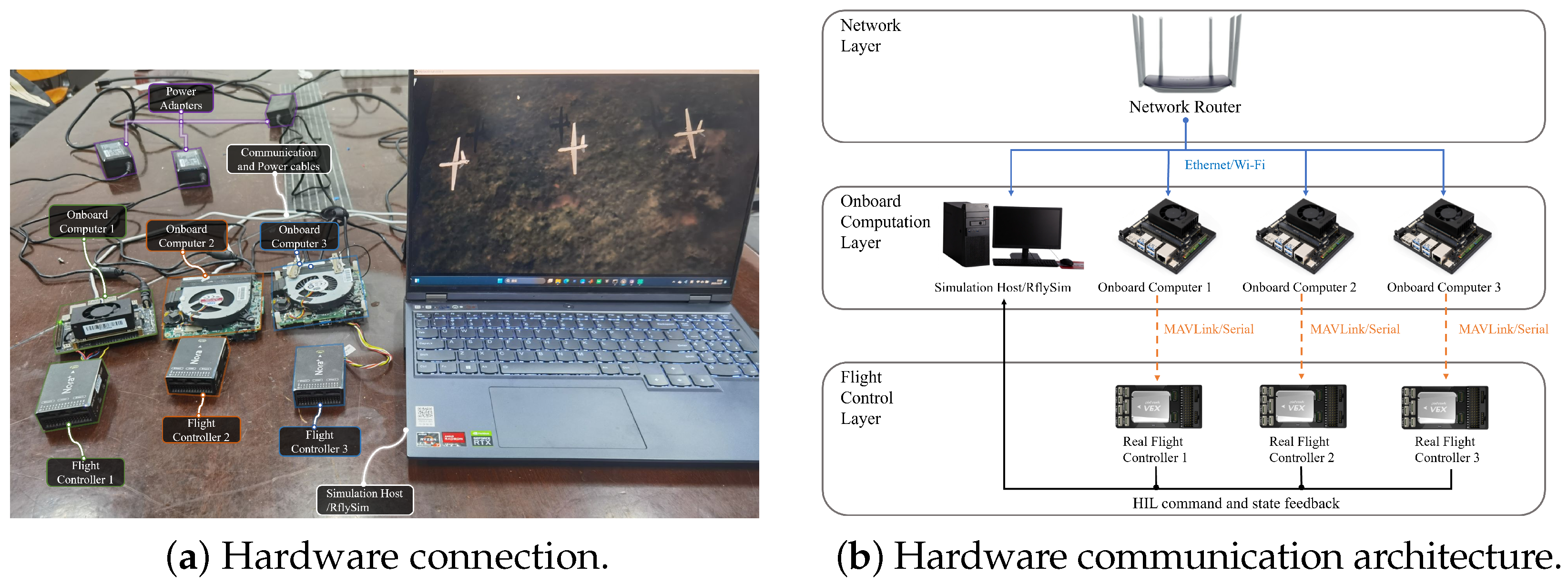
The HIL platform consists of a CUAV-NORA V6X flight controller, an NVIDIA Jetson Orin NX onboard computer, and a simulation host running RflySim v4.10 [30]. The onboard computer executes the trained SAC policy and generates a complete path from the current UAV state to the target. The resulting path is represented as a waypoint sequence for PX4 execution. ROS and MAVROS provide the interface between the onboard computer and PX4, while RflySim supplies the virtual mission scene, UAV dynamics, and simulated IMU/GPS feedback. Table 7 summarizes the platform and scenario settings, and Figure 15 shows the hardware connection and communication architecture.

Table 7. Semi-physical HIL platform and scenario configuration.

Category	Item	Configuration
Hardware	Flight controller	CUAV-NORA V6X
Hardware	Onboard computer	NVIDIA Jetson Orin NX
Software	Middleware	ROS with a MAVROS interface to PX4
Software	Simulator	RflySim v4.10
Simulation scene	Mission area	$100\mathrm{km}\times 100\mathrm{km}$ terrain used in the numerical simulations
Simulation scene	Cases	Scenario 1 with five radars and Scenario 2 with two radars
Scenario geometry	Radar and UAV states	Radar positions and initial/target positions follow Table 1
Simulation settings	Radar model	$C_d=-0.1{\mathrm{m}}^2{\mathrm{km}}^{-4}$ and $R_{\det }=12\mathrm{km}$
Simulation settings	Vehicle limits	$V=30–40\mathrm{m}/\mathrm{s}$ and $R_{\mathrm{safe}}=100\mathrm{m}$
Validation protocol	Repeated runs	10 runs per scenario, 20 runs in total

Figure 15. Semi-physical simulation platform: hardware connection and communication architecture.

The HIL scenarios use the mission geometry, terrain, initial and terminal states, modeled radar configuration, flight-speed range, and planning constraints specified for the numerical experiments. The numerical and HIL evaluations therefore share the same scenario-level parameter set.

For each HIL run, the trained SAC policy on the Jetson Orin NX generates one complete planned path before flight execution. The complete path is represented as a waypoint sequence and transferred to PX4. RflySim propagates the UAV dynamics and returns simulated state and sensor feedback during path execution. The SAC-generated load-factor and roll-angle variables are used only within the high-level path planner and are not transmitted directly as actuator commands. The HIL evaluation therefore examines one-shot offline path planning, waypoint transfer, and PX4 closed-loop execution rather than online replanning.

4.3.2. HIL Results and Analysis

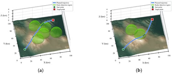
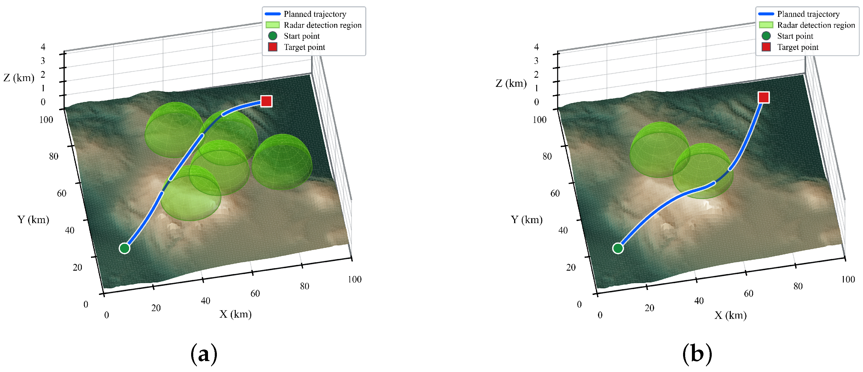
Figure 16 shows the HIL flight paths obtained for the two numerical configurations. Scenario 1 contains five modeled radar regions, whereas Scenario 2 contains two. In both cases, the planned path is represented as a waypoint sequence and executed by PX4 in the closed-loop HIL environment.

Figure 16. HIL flight paths for the five-radar and two-radar numerical scenarios. (a) Scenario 1 with five modeled radar regions. (b) Scenario 2 with two modeled radar regions.

Each HIL scenario was repeatedly tested 10 times. For consistency with the numerical evaluation, four quantities were recorded in every run: penetration time $t_{\mathrm{p}}$, average modeled radar-detection probability $P_{\mathrm{D}}^{\mathrm{avg}}$, average radar cross-section ${\sigma }^{\mathrm{avg}}$, and path-planning time $t_{\mathrm{a}}$. Here, $t_{\mathrm{a}}$ is the wall-clock time required by the Jetson Orin NX to complete one path-planning run. The scenario-wise means are summarized in Table 8.

Table 8. HIL evaluation results for the five-radar and two-radar scenarios.

Scenario	Runs	Mean Penetration Time ${\mathit{t}}_{\mathbf{p}}$ (s)	Mean Detection Probability ${\mathit{P}}_{\mathbf{D}}^{\mathbf{avg}}$	Mean RCS ${\mathit{\sigma }}^{\mathbf{avg}}$ (m2)	Mean Planning Time ${\mathit{t}}_{\mathbf{a}}$ (s)
Scenario 1	10	2728.05	0.0492	6.6586	5.13
Scenario 2	10	2712.36	0.0414	6.5423	4.96

These HIL tests are used to verify onboard execution of the planning algorithm, waypoint transfer, PX4 closed-loop tracking, and software–hardware communication in the two representative numerical scenarios.

5. Conclusions

This paper investigates the low-altitude penetration path planning problem for fixed-wing UAVs in complex battlefield environments with mountainous terrain and radar threats. To characterize the penetration process more realistically, a fixed-wing UAV dynamic model, a radar detection probability model, and a dynamic radar cross-section (RCS) model are developed. On this basis, the penetration task is formulated as a partially observable Markov decision process (POMDP), and a deep-reinforcement-learning-based path planning framework is proposed.

In the proposed framework, the Soft Actor-Critic (SAC) algorithm is employed to solve the dynamic-RCS-aware penetration planning problem. The observation space, action space, and reward function are carefully designed to jointly account for time efficiency, radar-threat avoidance, obstacle avoidance, and successful task completion. By incorporating dynamic RCS characteristics into the reinforcement learning framework, the proposed method enables the UAV to adapt its path and attitude in a coordinated manner, thereby reducing radar exposure risk while maintaining penetration-time performance.

Simulations show dynamically feasible flight paths under the adopted models. Among the successful trials of each method, SAC achieves the shortest mean penetration time and lower mean computation time than A* and the pseudo-spectral method, but higher computation time than PPO. In this comparison, the pseudo-spectral method and PPO yield lower mean exposure metrics than SAC, indicating a trade-off rather than general superiority. In addition, comparative experiments under dynamic and static RCS settings further demonstrate the importance of incorporating dynamic RCS characteristics into the path planning process. HIL tests in the corresponding five-radar and two-radar numerical scenarios support onboard one-shot path planning, waypoint transfer, and PX4 closed-loop execution.

The evaluation uses one weighting configuration and a fixed SAC policy for each mission-level comparison, and it does not include a matched NMPC baseline. It therefore does not establish weight sensitivity, Pareto behavior, reward-ablation effects, anisotropy sensitivity, statistical significance, or relative performance against NMPC under a common model. The exact computing-device model and some original software-version metadata were not retained, although all compared methods were timed on the same device. The robustness and reproducibility of SAC training are characterized by the across-seed mean and standard deviation over 100 independent training runs. For the mission-level evaluation, continuous metrics are summarized as means with standard deviations over the method-specific successful trials, whereas success, collision, and timeout rates are reported over all 100 shared stochastic scenarios.

The feedforward SAC policy uses current partial observations and does not explicitly resolve partial observability through memory or state estimation. The RCS model is not calibrated to the airframe, and the RCS and radar-risk models remain planning-level parameterizations without frequency-, polarization-, or vehicle-specific calibration. Sensing errors and physical energy are not modeled. Detection probability therefore represents modeled exposure rather than measured survivability. The HIL experiments verify functional software–hardware integration and are not interpreted as independent validation of the physical radar model or full-scale aerodynamic performance.

Future work will address outdoor flight, uncertain radar information, RCS calibration and sensitivity, energy-aware objectives, nested analyses separating training-seed and test-scenario effects, weight sensitivity, Pareto and reward-ablation analyses, anisotropy-sensitivity studies, and matched NMPC comparisons.

References

- Li, Y.; Shi, C.; Yan, M.; Zhou, J. Mission planning and trajectory optimization in UAV swarm for track deception against radar network. Remote Sens. 2024, 16, 3490. [Google Scholar] [CrossRef] [Scilit]
- Aggarwal, S.; Kumar, N. Path planning techniques for unmanned aerial vehicles: A review, solutions, and challenges. Comput. Commun. 2020, 149, 270–299. [Google Scholar] [CrossRef] [Scilit]
- Yu, Z.; Si, Z.; Li, X.; Wang, D.; Song, H. A novel hybrid particle swarm optimization algorithm for path planning of UAVs. IEEE Internet Things J. 2022, 9, 22547–22558. [Google Scholar] [CrossRef] [Scilit]
- Zhang, Z.; Wu, J.; Dai, J.; He, C. Optimal path planning with modified A-Star algorithm for stealth unmanned aerial vehicles in 3D network radar environment. Proc. Inst. Mech. Eng. Part G J. Aerosp. Eng. 2022, 236, 72–81. [Google Scholar] [CrossRef] [Scilit]
- Yang, Z.; Yuan, Z.; Wang, X.; Huang, J.; Zhou, D. Autonomous control of UAV trajectory based on RHC-Radau method in complex penetration combat environment. Aerosp. Sci. Technol. 2024, 146, 108915. [Google Scholar] [CrossRef] [Scilit]
- Fu, J.; Sun, G.; Yao, W.; Wu, L. On trajectory homotopy to explore and penetrate dynamically of multi-UAV. IEEE Trans. Intell. Transp. Syst. 2022, 23, 24008–24019. [Google Scholar] [CrossRef] [Scilit]
- Lim, J.; Achermann, F.; Girod, R.; Lawrance, N.; Siegwart, R. Safe low-altitude navigation in steep terrain with fixed-wing aerial vehicles. IEEE Robot. Autom. Lett. 2024, 9, 4599–4606. [Google Scholar] [CrossRef] [Scilit]
- Luo, J.; Liang, Q.; Li, H. UAV penetration mission path planning based on improved holonic particle swarm optimization. J. Syst. Eng. Electron. 2023, 34, 197–213. [Google Scholar] [CrossRef] [Scilit]
- Bianchi, D.; Borri, A.; Di Gennaro, S.; Preziuso, M. UAV trajectory control with rule-based minimum-energy reference generation. In Proceedings of the 2022 European Control Conference (ECC), London, UK, 12–15 July 2022; pp. 1497–1502. [Google Scholar] [CrossRef] [Scilit]
- Yuan, J.; Liu, Z.; Lian, Y.; Chen, L.; An, Q.; Wang, L.; Ma, B. Global optimization of UAV area coverage path planning based on good point set and genetic algorithm. Aerospace 2022, 9, 86. [Google Scholar] [CrossRef] [Scilit]
- Chen, D.; Xu, L.; Wang, C. An advanced control method for aircraft carrier landing of UAV based on CAPF–NMPC. Aerospace 2024, 11, 656. [Google Scholar] [CrossRef] [Scilit]
- Lu, J.; Zhang, X.; Shen, H.; Xu, L.; Tian, B. You only plan once: A learning-based one-stage planner with guidance learning. IEEE Robot. Autom. Lett. 2024, 9, 6083–6090. [Google Scholar] [CrossRef] [Scilit]
- Wang, Z.; Ng, S.X.; El-Hajjar, M. Deep reinforcement learning assisted UAV path planning relying on cumulative reward mode and region segmentation. IEEE Open J. Veh. Technol. 2024, 5, 737–751. [Google Scholar] [CrossRef] [Scilit]
- Alpdemir, M.N. Tactical UAV path optimization under radar threat using deep reinforcement learning. Neural Comput. Appl. 2022, 34, 5649–5664. [Google Scholar] [CrossRef] [Scilit]
- Xue, Y.; Chen, W. A UAV navigation approach based on deep reinforcement learning in large cluttered 3D environments. IEEE Trans. Veh. Technol. 2023, 72, 3001–3014. [Google Scholar] [CrossRef] [Scilit]
- Xi, M.; Dai, H.; He, J.; Li, W.; Wen, J.; Xiao, S.; Yang, J. A lightweight reinforcement-learning-based real-time path-planning method for unmanned aerial vehicles. IEEE Internet Things J. 2024, 11, 21061–21071. [Google Scholar] [CrossRef] [Scilit]
- Bao, L.; Guo, Z.; Gao, X.; Li, C. Stealth UAV Path Planning Based on DDQN Against Multi-Radar Detection. Aerospace 2025, 12, 774. [Google Scholar] [CrossRef] [Scilit]
- Li, J.; Zhang, T.; Liu, K. Memory-Enhanced Twin Delayed Deep Deterministic Policy Gradient (ME-TD3)-Based Unmanned Combat Aerial Vehicle Trajectory Planning for Avoiding Radar Detection Threats in Dynamic and Unknown Environments. Remote Sens. 2023, 15, 5494. [Google Scholar] [CrossRef] [Scilit]
- Hu, J.; Fan, L.; Lei, Y.; Xu, Z.; Fu, W.; Xu, G. Reinforcement learning-based low-altitude path planning for UAS swarm in diverse threat environments. Drones 2023, 7, 567. [Google Scholar] [CrossRef] [Scilit]
- Xu, Q.; Ge, J.; Yang, T.; Sun, X. A trajectory design method for coupling aircraft radar cross-section characteristics. Aerosp. Sci. Technol. 2020, 98, 105653. [Google Scholar] [CrossRef] [Scilit]
- Liu, X.; Yin, Y.; Su, Y.; Ming, R. A multi-UCAV cooperative decision-making method based on an MAPPO algorithm for beyond-visual-range air combat. Aerospace 2022, 9, 563. [Google Scholar] [CrossRef] [Scilit]
- Fang, X.L.; Yang, Y.X. Radar target detection range model based on detection probability. Mod. Radar 2008, 7, 18–20. [Google Scholar]
- Zhang, Z.; Jiang, J.; Wu, J.; Zhu, X. Efficient and optimal penetration path planning for stealth unmanned aerial vehicle using minimal radar cross-section tactics and modified A-Star algorithm. ISA Trans. 2023, 134, 42–57. [Google Scholar] [CrossRef] [Scilit]
- Alagoz, O.; Hsu, H.; Schaefer, A.J.; Roberts, M.S. Markov decision processes: A tool for sequential decision making under uncertainty. Med. Decis. Mak. 2010, 30, 474–483. [Google Scholar] [CrossRef] [Scilit] [PubMed]
- Kurniawati, H. Partially observable Markov decision processes and robotics. Annu. Rev. Control Robot. Auton. Syst. 2022, 5, 253–277. [Google Scholar] [CrossRef] [Scilit]
- Haarnoja, T.; Zhou, A.; Abbeel, P.; Levine, S. Soft actor-critic: Off-policy maximum entropy deep reinforcement learning with a stochastic actor. In Proceedings of the 35th International Conference on Machine Learning, Stockholm, Sweden, 10–15 July 2018; Volume 80, pp. 1861–1870. [Google Scholar]
- Khalaf-Allah, M. Emitter Location with Azimuth and Elevation Measurements Using a Single Aerial Platform for Electronic Support Missions. Sensors 2021, 21, 3946. [Google Scholar] [CrossRef] [Scilit] [PubMed]
- Wu, G.; Guo, F.; Zhang, M. Direct Position Determination: An Overview. J. Radars 2020, 9, 998–1013. [Google Scholar] [CrossRef]
- Ng, A.Y.; Harada, D.; Russell, S.J. Policy invariance under reward transformations: Theory and application to reward shaping. In Proceedings of the 16th International Conference on Machine Learning, Bled, Slovenia, 27–30 June 1999; pp. 278–287. [Google Scholar]
- Wang, S.; Dai, X.; Ke, C.; Quan, Q. RflySim: A rapid multicopter development platform for education and research based on Pixhawk and MATLAB. In Proceedings of the 2021 International Conference on Unmanned Aircraft Systems (ICUAS); IEEE: New York, NY, USA, 2021; pp. 1587–1594. [Google Scholar] [CrossRef] [Scilit]
Disclaimer/Publisher’s Note: The statements, opinions and data contained in all publications are solely those of the individual author(s) and contributor(s) and not of MDPI and/or the editor(s). MDPI and/or the editor(s) disclaim responsibility for any injury to people or property resulting from any ideas, methods, instructions or products referred to in the content. |
© 2026 by the authors. Licensee MDPI, Basel, Switzerland. This article is an open access article distributed under the terms and conditions of the Creative Commons Attribution (CC BY) license.