


Abstract
The detection of orbital anomalies is of critical importance to the safe operation of on-orbit spacecraft. Existing methods often rely on manually engineered features and are constrained by the limited computational resources of satellite equipment. This paper proposes a lightweight unsupervised anomaly detection method based on the Peak Adversarial Autoencoder (Peak-AAE). First, the Peak-AAE model is employed to reconstruct historical semi-major axis data, and the squared differences between the reconstructed and original data are taken as the residual sequence. The Automatic Multi-Scale Peak Detection (AMPD) algorithm is then applied to the residual sequence to identify anomalous points. In comparison with traditional approaches, this method eliminates the need for manual feature design. Moreover, the improved Peak-AAE model effectively reduces the false positive rate associated with the original AAE model, thereby enhancing detection accuracy. Finally, the compressed Peak-AAE model is deployed on edge devices for ground simulation verification. Experimental validation on the BEIDOU-3 G2 and IRNSS-1A satellites demonstrates that the Peak-AAE model achieves a minimum precision of 90.00% and a minimum recall of 84.74%.
1. Introduction
The anomalies in the orbits of space objects can be broadly categorized into three types: first, maneuvers controlled by human intervention; second, special events that occur without human involvement, such as collisions between space objects or fuel leaks from spacecraft; and third, anomalies caused by extreme space environments affecting spacecraft [1]. Among the three types of orbital anomalies, orbital maneuver data are the most abundant and have detailed historical records; therefore, this paper primarily takes orbital maneuvers as the research object for anomaly detection. The variation in the orbital parameters of a spacecraft can be used to identify whether the spacecraft has experienced an anomaly. Under normal conditions, the changes in these parameters are very small. However, when an anomaly occurs, the changes in the parameters become more significant. There are two types of parameter variations: in-plane changes and out-of-plane changes. When the change occurs within the same orbital plane, the semi-major axis changes most noticeably. When the change occurs in a different orbital plane, the orbital inclination changes more significantly [2]. Common methods for identifying orbital anomalies typically process the two aforementioned characteristics, construct new features that are easier to recognize, and finally use threshold-based methods to identify anomalous points. Patera was the first to propose a data fitting method based on a sliding window for spatial event detection. This method subtracts the fitted data from the actual data within the window to obtain the deviation data, calculates the mean, variance, and standard deviation of the deviation data, and uses the standard deviation as the threshold. If the threshold is exceeded, an event is declared [3]. Cao et al. addressed the issue of orbital anomalies by applying the concept of dynamic optimization. They segmented the data by assuming the presence of anomaly points, calculated the loss within each segment, and through iterative optimization, obtained the distribution of anomaly points under the condition of the minimum total loss within the segments. These points were identified as the actual anomaly points [4]. Song et al. proposed an orbit anomaly detection method called the “Semi-Major Axis Change Method”, which employs the deviation of the semi-major axis from a reference point as the detection feature. The decision threshold is defined as k multiplied by the summation of the mean absolute deviation of semi-major axis variations and three sigma of the statistical distribution [5]. Yan et al., considering the limitations of the single-feature method, proposed a discrimination method that integrates three features—the absolute value of the change in semi-major axis of the orbit, the absolute value of the rate of change of the semi-major axis of the orbit, and the discrete ratio of the mean motion of the orbit—called the comprehensive criterion method. This method sets different criteria for different satellites. Experimental results show that the comprehensive criterion method effectively eliminates missed judgments on LEOs and maintains a high accuracy rate [6]. Mukundan and Wang proposed an anomaly detection method that compares the actual Two-Line Element (TLE) orbital elements with the predicted orbital elements obtained from a simplified perturbation model. The detection feature is derived from the difference between these two sets of orbital elements. The effectiveness of the anomaly detection depends on the selection of the detection window size and the threshold value [7]. Qin et al. designed a function to fit the orbital parameters of satellites, based on the long-term and short-term operational patterns of these parameters. Taking the semi-major axis as an example, anomaly detection is performed by comparing the short-term periodic values of the fitted semi-major axis with the actual observed values [8]. Su Jianmin used the difference in specific mechanical energy between the space object and the spacecraft as a feature for maneuver identification, applied wavelet transform to process noisy signals, and finally performed anomaly detection [9].
As can be seen from the above, existing research is relatively traditional and generally proceeds in two steps:
Step 1: Designing new features that are easy to identify. This can be based on the intrinsic relationships between data, such as the change or rate of change of the semi-major axis, or other methods, such as using the deviation between the predicted values from the SGP4/SDP4 model and the actual values as identification features, or using the deviation between the polynomial fitting results and the actual values as features.
Step 2: Using threshold detection methods to detect anomalies. In this step, the most common method is the fixed threshold approach, which identifies anomalies by combining the mean and standard deviation of the feature, or by using a sliding window for identification. However, these methods require tuning the threshold value or the window length. In short, they are all methods with hyperparameters that require manual search for the optimal parameters.
Meanwhile, deep learning methods have been widely applied in related fields. References [10,11,12,13] utilized neural networks for anomaly detection in telemetry signals. Reference [14] employed recurrent neural networks to detect anomalies in data streams. Chen et al. applied autoencoders for unsupervised anomaly detection [15]. Li et al. proposed a GAN-based multivariate anomaly detection method used for identifying anomalies in cyber–physical systems [16]. Zong et al. introduced a deep autoencoding Gaussian mixture model for unsupervised anomaly detection, primarily targeting high-dimensional data [17].
The success of deep learning methods in the field of anomaly detection has motivated this work to apply them to orbit anomaly detection. To reduce human intervention, we employ an adaptive, threshold-free detection method—AMPD—in place of a manually designed detection function. In short, this paper constructs identification features using deep learning methods and detects anomalies through a threshold-free detection function. It should be noted that while the network model contains hyperparameters during its construction and training phase, this is separate from the detection function, which itself operates without any hyperparameters.
The innovations of this paper are as follows:
- Orbital anomalies are typically of short duration and manifest as a steep peak immediately followed by a valley. The onset phase corresponds to the peak, while the end phase corresponds to the valley (or vice versa), yet both phases deviate from normal data. Under these conditions, conventional reconstruction models (e.g., VAE, GAN, Transformer) are incapable of distinguishing between the onset and end phases of an orbital anomaly and may randomly identify either phase as anomalous, resulting in false detections [18,19,20]. To address this limitation, we introduce a peak probability generation module that computes the peak probability for each data point. During the training of the Adversarial Autoencoder (AAE), a non-peak loss term is constructed based on these probabilities, which enhances the reconstruction accuracy at peak regions and thereby prevents false detections.
- To overcome the issues of index out-of-bounds errors at the boundaries and missed detections of anomalies located at both ends of the data sequence in the original AMPD algorithm, two optimizations are proposed: first, the index search range for peak detection is restricted to avoid out-of-bounds errors; second, edge padding is applied to both ends of the data sequence to ensure that anomalies occurring at the extremities are fully captured.
- To satisfy the real-time inference requirements of on-orbit edge devices, the Peak-AAE model is further compressed through lightweight optimization. The total number of model parameters is reduced from approximately 48k to about 9.3k, the model size is decreased from 201 KB to 52 KB, and the maximum degradation in detection accuracy is limited to 2.85%.
The rest of this paper is organized as follows: In Section 2, the orbit anomaly detection method is introduced in detail, including the network architecture of the Peak Adversarial Autoencoder, its training process, and modifications to the AMPD algorithm. In Section 3, the proposed method is tested on BEIDOU-3 G2 and IRNSS-1A satellites and compared with other traditional methods to verify whether the algorithm is efficient, as well as being compared with the original AAE model to verify whether the improved method is effective. Section 4 describes the edge deployment of the lightweight orbit anomaly detection system based on compressed Peak-AAE. In Section 5, the proposed method is summarized.
2. Orbit Anomaly Detection Method
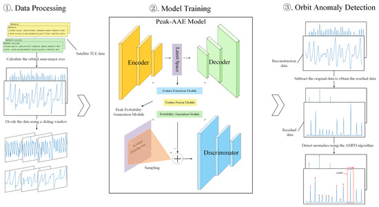
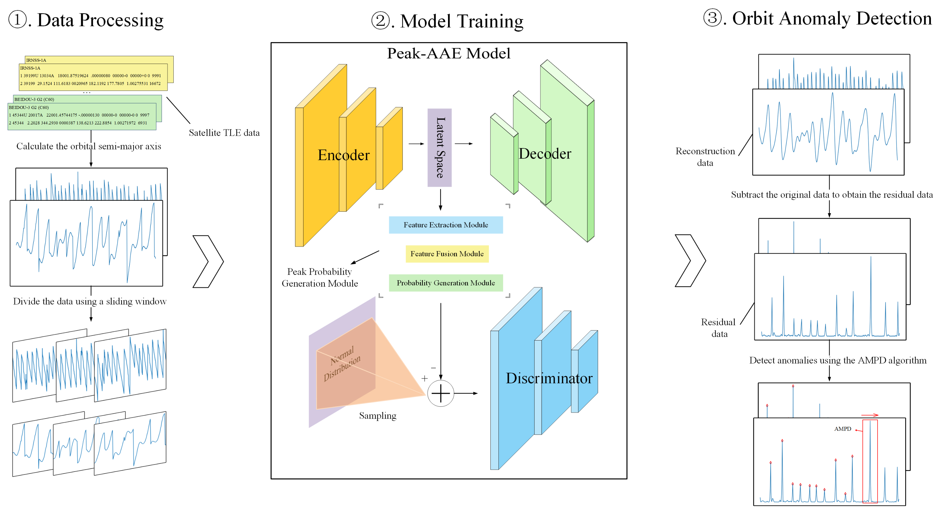
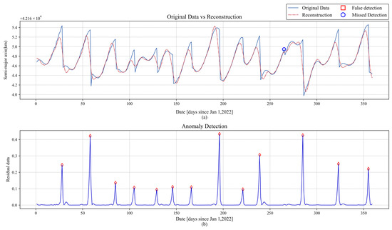
The anomaly detection framework proposed in this paper is shown in Figure 1, and it is mainly divided into three parts: data processing, model training, and orbit anomaly detection. First, historical TLE data of the target satellite is obtained from Space-Track, and based on this, the historical semi-major axis of the orbit is calculated. The data is then segmented using a sliding window. Next, the processed data is input into the model for training. The first step is to train the peak probability generation module to generate peak probabilities for each data point, which will be used for subsequent autoencoder training. The second step is to fix the autoencoder and train the discriminator. The third step is to fix the discriminator and train the autoencoder. The detailed training parameters for the three modules are shown in Table 1. Finally, the Peak-AAE model is used to reconstruct the data, and the squared difference between the reconstructed data and the original data is calculated as the residual data. The AMPD algorithm is then used to detect anomalies.
Figure 1.
Framework diagram of anomaly detection methods.
Table 1.
Training parameters.
2.1. Data Processing
The TLE data is created by the North American Aerospace Defense Command (NORAD) to describe the orbital parameters of artificial satellites. Each satellite’s TLE contains two lines of data, each with 69 characters, including the satellite’s designation, orbital inclination, right ascension of the ascending node, eccentricity, argument of perigee, mean anomaly, and mean motion, among other parameters. Although the semi-major axis of the orbit is not directly provided, it can be calculated from the mean motion of the orbit.
First, according to the 53rd to 63rd bits in the second line of the TLE data, we obtain the number of revolutions that a satellite completes around the Earth per day, denoted as n (revolutions/day). Taking the reciprocal of this value gives the orbital period T1 (days/revolution):
Convert units to (seconds/revolution):
According to Kepler’s third law,
The semi-major axis of the orbit is
The gravitational constant G is the standard Earth gravitational constant, M is the Earth’s mass, and the product equals 398,600.4418 km3/s2.
A window of length m with a stride of 1 is used to segment the historical semi-major axis data. Assuming that the length of the historical data is L, the resulting data form a two-dimensional array of size . After applying Z-score normalization to this array, the data are loaded into a neural network model by a dataloader with a specified batch size. The normalization formula is given as follows:
where is the normalized value, X is the original value, is the mean, and is the standard deviation.
2.2. Network Structure
Adversarial Autoencoder is a deep learning model that combines Autoencoder (AE) and Generative Adversarial Networks (GANs). In the AAE model, the encoder E maps the distribution of input data x to a latent space Z. This mapping is trained adversarially with samples drawn from a given prior distribution , so that the aggregated posterior distribution generated by the encoder matches the given prior distribution . In this paper, we use a normal distribution as the given prior distribution . Finally, the posterior distribution is related to the conditional distribution , which maps the input data X to the latent space Z. Here, denotes the distribution of the input data x [21].
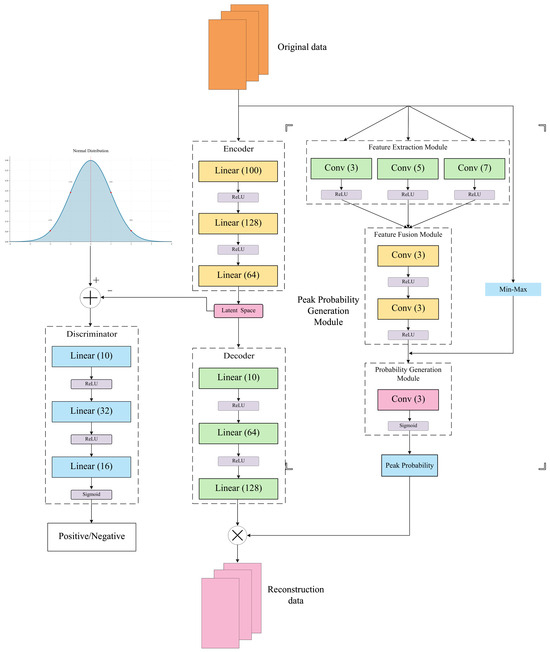
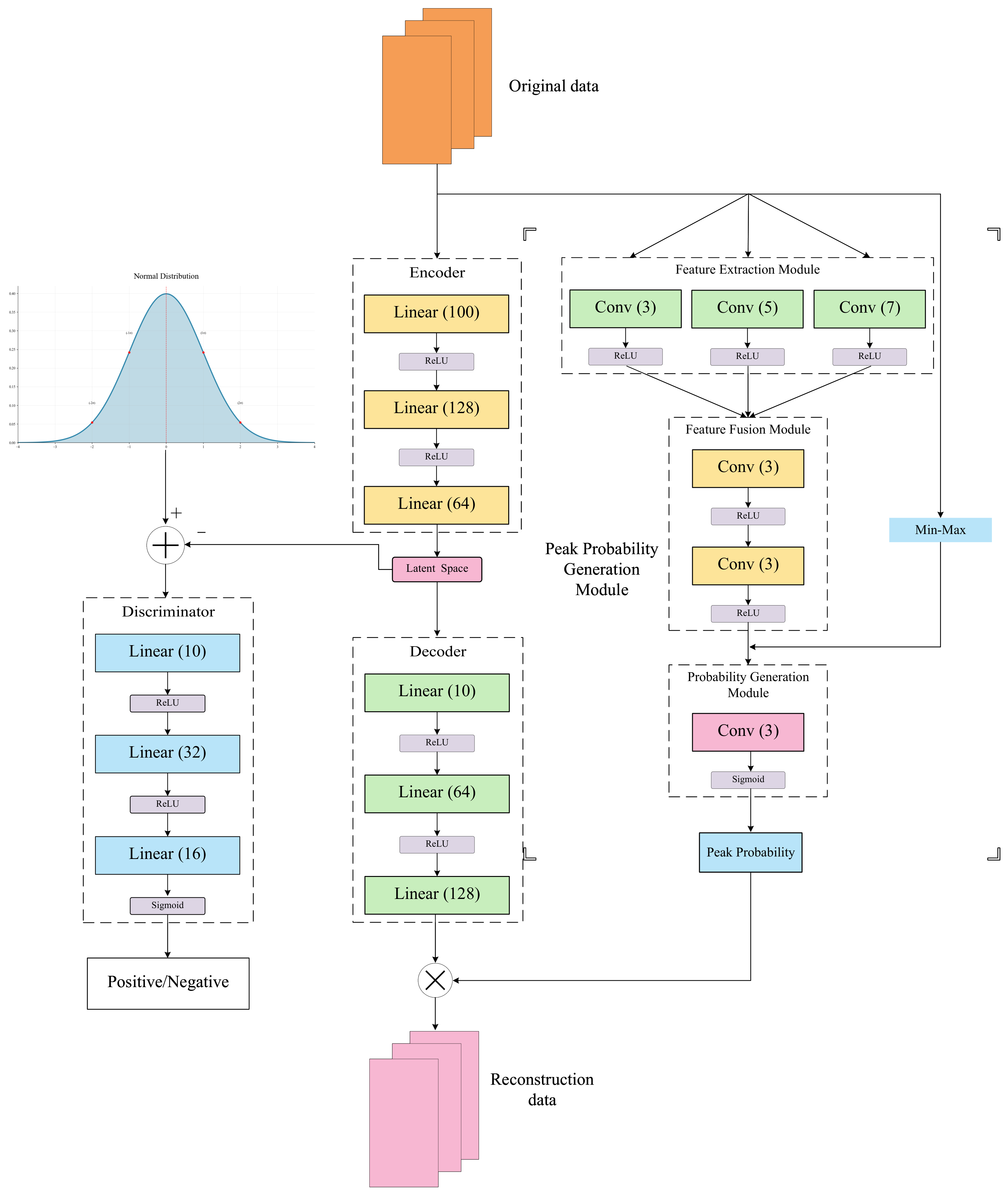
The original AAE model comprises an encoder (E), a decoder (G), and a discriminator (D). Building upon this foundation, we have incorporated a peak probability generation module, which consists of three sub-modules. The detailed structure is illustrated in Figure 2.
Figure 2.
Peak-AAE structure diagram.
The peak probability generation module consists of three sub-modules: a feature extraction module, a feature fusion module, and a probability generation module. The feature extraction module comprises three one-dimensional convolutional layers with different kernel sizes (3, 5, 7), which capture feature information at different scales. The feature fusion module consists of two one-dimensional convolutional layers with a kernel size of 3. It combines the outputs of the aforementioned three convolutional layers to achieve feature fusion and reduces the number of parameters through two consecutive convolutional operations. Finally, the probability generation module outputs the peak probability for each point via a Sigmoid function. The mathematical expression of the one-dimensional convolutional layer is as follows:
where k represents the kernel size, s denotes the stride, p indicates the padding, and b stands for the bias.
The encoder E and the decoder G are both composed of two 3-layer MLPs (Multi-Layer Perceptrons). Together, they form an Autoencoder, which aims to minimize the deviation between the reconstructed data and the original data, thereby learning the normal patterns of the original data [22]. This can be represented by the following formula:
The notation represents the weight matrix of the n-th layer, and represents the bias vector of the n-th layer. The notation denotes the activation function of the n-th layer, and x is the input data. Among them, and are both ReLU functions, whose expressions are as follows:
The discriminator is similar to the aforementioned model, with its activation function being the Sigmoid function, used to output the probability of whether the latent vector comes from the prior distribution or the encoded distribution. Its expression is as follows:
2.3. Training Algorithm
2.3.1. Training Process of the Peak Probability Module
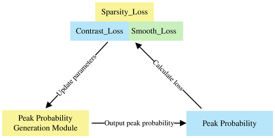
To address the issue that the original reconstruction model cannot distinguish between the onset and termination phases of orbit anomalies, we propose to resolve this by achieving different reconstruction accuracies at peak and non-peak regions. The probabilities generated by the peak probability generation module for each point serve as the basis for distinguishing between peaks and non-peaks. This module operates in an unsupervised learning manner, trained under three constraints—sparsity, smoothness, and contrast—defined as follows:
Peak_probi represents the peak probability of point i. Sparsity_Loss denotes the mean value of the peak probabilities, which is expected to be small (since only a few points are peaks). Peak_prob[2,n] represents the peak probabilities from point 2 to n, and peak_prob[1,n−1] represents the peak probabilities from point 1 to n−1. The MSE calculates the mean square error between the two sequences. Smooth_Loss reflects the difference in peak probability between two adjacent positions; since the peak probabilities of neighboring points should be similar, this value should also be small. Min_max denotes min–max normalization. which is defined as follows:
where is the normalized value, is the minimum value of the input sequence, and is the maximum value of the input sequence.
Contrast_Loss indicates that the probability of a point being a peak is positively correlated with its magnitude; the larger the value, the more likely it is to be a peak. The training procedure is shown in Figure 3.
Figure 3.
Peak probability module training.
It is worth noting that the peak probability module differs from the traditional attention mechanism. The attention mechanism primarily operates on the feature representation layer, altering features by learning attention weights and multiplying them with the features. In contrast, the peak probability module generates the peak probability for each point through an unsupervised method. During loss computation, it provides a judgment on the importance of each point location, thereby enhancing the discrimination of each point and avoiding false detections.
2.3.2. Training Process of the Discriminator
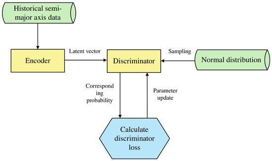
Fix the weights of the Autoencoder, and input historical semi-major axis data into the encoder to generate corresponding latent vectors. These latent vectors are then combined with samples from a normal distribution (given prior distribution) and input into the discriminator. The discriminator outputs the probability that the input comes from the prior distribution. Finally, the loss is calculated using BCELoss (binary cross-entropy loss), and the parameters of the discriminator are updated. The flowchart is shown in Figure 4.
Figure 4.
Discriminator training.
The loss function is defined as follows:
denotes the binary cross-entropy loss between x and y, indicates that the data is sampled from the true distribution, represents the discriminator’s judgment output, and stands for the latent vector generated by the encoder. When the discriminator D achieves perfect discrimination , , the total loss becomes zero.
2.3.3. Training Process of the Autoencoder
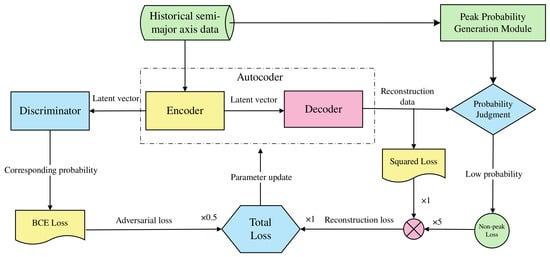
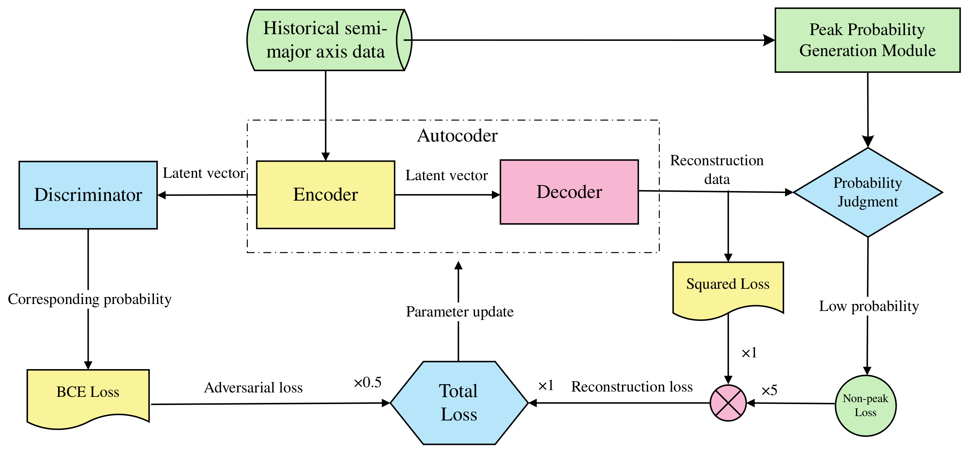
Input semi-major axis data into the encoder to generate latent vectors. These latent vectors are then fed into both the discriminator and the decoder. The discriminator outputs the probability that the vector originates from prior sampling and computes the binary cross-entropy of this probability as the adversarial loss. The decoder generates reconstructed data based on the latent vector, using the squared error between the original data and the reconstructed data as the basic reconstruction loss. Peaks are identified based on the point-wise probabilities generated by the peak probability generation module, where points with probabilities below the mean are classified as non-peaks, and those above the mean as peaks. An additional loss is calculated for non-peak points, referred to as the non-peak loss. The final reconstruction loss is the sum of five times the non-peak loss and the basic reconstruction loss. The total loss is obtained by adding the reconstruction loss and 0.5 times the adversarial loss, after which the Autoencoder parameters are updated. The flowchart is shown in Figure 5.
Figure 5.
Autoencoder training.
Mathematical expression of reconstruction loss:
Mathematical expression of adversarial loss:
Mathematical expression of the total loss function:
represents the encoder E mapping the input x to a latent vector. represents the decoder G reconstructing the data from the latent vector, represents the discriminator judgment on the latent vector generated by the encoder E, denotes the positions of non-peak points, represents the basic reconstruction loss, denotes the non-peak loss, represents the total reconstruction loss, denotes the adversarial loss, and represents the total loss.
2.4. Optimize the AMPD Algorithm
The original AMPD algorithm first constructs the LMS (Local Maximum Scale) map, calculates the row-wise sum to obtain the vector , and selects the scale corresponding to the minimum row sum as the optimal scale . Peaks are identified as extrema satisfying scales 1 through . While theoretically applicable for peak detection, this algorithm has certain limitations in practical applications. When constructing the LMS map, its elements are defined as follows:
When , an index out-of-bounds error may occur. If we directly restrict i to , it may lead to missed detections at the ends of the data. An effective solution is to restrict i to when searching for the optimal scale, as the data length is usually much larger than the optimal scale and, thus, has a minimal impact on scale selection. During peak detection, edge padding is applied to both ends of the detected data, with the padding length equal to the optimal scale and the padding values set to the mirror values of the edges. This approach effectively avoids missed detections, and only when the first or the last point happens to be an edge maximum will it be falsely detected, making it convenient for users to determine whether the padding has introduced any false detection points.
3. Experiment and Analysis
In this section, we will test the anomaly detection method of the Peak-AAE model on satellites. First, we introduce the experimental data and evaluation metrics, and then we conduct comparative experiments using the proposed method along with traditional methods and network models. We perform ablation studies with the original AAE model and the AMPD algorithm to investigate the effectiveness of the relevant modifications. Finally, we analyze and summarize the experimental results.
3.1. Data Description
Our test subjects are BEIDOU-3 G2 and IRNSS-1A, both of which are navigation satellites in GEO (Geostationary Earth Orbit). Compared to other satellites, GEO satellites experience more frequent orbital changes due to the resonance caused by Earth’s rotation. As a result, they have abundant orbital maneuver history data, making them well suited for orbit anomaly detection.
For the BEIDOU-3 G2 satellite, we tested its TLE data from 1 January 2022 to 31 December 2022. The maneuver history was referenced from [23]. However, TLE data for days 130, 168, 169, 200, 227, and 229 are missing. Therefore, these days were excluded from the original satellite maneuver timeline. Additionally, the maneuver on day 198 was adjusted to day 196 based on actual changes in the semi-major axis. Observations of the semi-major axis indicate that no maneuver occurred on day 198, whereas a significant change was detected on the adjacent day 196, leading to the aforementioned adjustment. The maneuver history records are shown in Table 2, where the numbers represent day-of-year (DOY) values.
Table 2.
BEIDOU-3 G2 maneuver history.
For the IRNSS-1A satellite, we tested its TLE data from 2018 to 2021. Due to the long observation period and poor observational conditions, the IRNSS-1A dataset exhibits more missing TLE entries. Additionally, since no reference maneuver history data was available, its anomaly points were manually identified. The results are presented in Table 3, where the numbers indicate the elapsed days from the first data point (1 January 2018), excluding any missing days. Due to the presence of missing data, these numbers do not correspond directly to the day-of-year. The criterion for manual detection is primarily based on the variation of the semi-major axis. First, calculate the difference in the semi-major axis between adjacent days. During normal satellite operation, the variation ranges from tens of meters to around a hundred meters, whereas when a maneuver occurs, the variation is typically in the order of several kilometers. A preliminary screening is performed using the principle to identify candidate points. After identifying candidate points, check the corresponding positions on the semi-major axis plot for peaks and troughs. If they are present, confirm the point as a maneuver point; if not, skip the candidate point.
Table 3.
IRNSS-1A maneuver history.
All data were obtained from Space-Track. For the sake of simplifying the experiment, the first TLE data updated each day (the latest one on that day) were used as the satellite orbital data. The reason for using the first TLE of each day is to keep the time intervals as similar as possible. Because the update frequency is irregular, if all TLE data were used as input, the differences between consecutive data points could fluctuate significantly due to the update frequency rather than the presence or absence of a maneuver, leading to false detections and missed detections. For the detection results, similar time intervals ensure that the differences between adjacent points remain close when the satellite operates normally, making it much easier to identify a maneuver when it occurs. At the same time, the problem of irregular TLE update frequency can be somewhat diluted over larger time intervals. Finally, since the magnitude of a maneuver is large, the inherent accuracy of the TLE itself does not have a significant impact on the experiment.
3.2. Evaluation Metric
We use precision, recall, and F1-score as evaluation metrics. The relevant formulae are shown in the following sections. We set anomalous points as the positive class and normal points as the negative class.
Precision: Measures the proportion of correctly predicted anomalous samples among all samples predicted as anomalous:
Recall: Measures the proportion of correctly identified anomalous samples among all actual anomalous samples:
F1-Score: The harmonic mean of precision and recall, providing a balanced evaluation of a model’s accuracy and completeness:
TP stands for predicted positive and actually positive, FP stands for predicted positive and actually negative, and FN stands for predicted negative and actually positive.
3.3. Comparative Experiment
We adopted the Moving-Window Curve Fitting (MWCF) method proposed by Patera and the Semi-Major Axis Change Method (SACM) proposed by W.D. Song as representatives of traditional approaches [3,5], while using VAE, USAD, and Anomaly-Transformer models as representative algorithms from the field of deep learning [18,24,25]. VAE and USAD exemplify two widely used deep learning architectures for anomaly detection (VAE, GAN), whereas the Transformer represents a more recently popularized model. To mitigate the impact of random initialization, data batch ordering, and stochastic processes during the training of deep learning models on the experimental results, we conducted five independent repeated experiments for all of the proposed deep learning comparison methods (VAE, USAD, and Anomaly-Transformer) under the same hyperparameter settings, using different system random seeds each time without manual fixing. The mean and standard deviation (mean ± std) of precision, recall, and F1-score are reported. Since MWCF and the SACM are traditional methods whose outputs—given fixed input data, window length, and threshold parameters—are unaffected by random initialization, only a single deterministic result is reported for them. For the MWCF method, a window length of 7 was used along with a third-order polynomial for fitting; the absolute value of the derivative at the beginning of the window was taken as the identification feature. Due to the poor performance of the threshold detection, it was replaced by AMPD. The detection results are shown in Table 4 and Table 5, and the corresponding t-distribution confidence intervals are provided in Appendix A (Table A1 and Table A2).
Table 4.
Comparative experiment results on BEIDOU-3 G2.
Table 5.
Comparative experiment results on IRNSS-1A.
As can be seen from Table 4 and Table 5, the SACM demonstrates commendable performance on both datasets. In the tests conducted on the two satellites, it achieved the highest recall rate, indicating a lower likelihood of missed detections by the model. While MWCF performs well on the BEIDOU-3 G2 satellite, its effectiveness is notably poorer on the IRNSS-1A satellite, with all three evaluation metrics failing to exceed 50%. This suggests that the applicability of the MWCF method is relatively limited. The results from VAE and USAD confirm a common issue with reconstruction-based models: their inability to distinguish between the onset and end phases of an orbit anomaly. These models tend to randomly identify either phase as anomalous, leading to final results fluctuating around 50%. Although some detection results from the Anomaly-Transformer do not strictly follow this pattern, the majority of its detection points still substantiate this conclusion. Finally, the method proposed in this paper exhibits superior overall performance compared to traditional orbit anomaly detection methods and common network models. In the test on the BEIDOU-3 G2 satellite, it attained a mean precision of 94.57% and an F1-score of 94.33%, outperforming the other five methods. Similarly, in the detection task for IRNSS-1A, it achieved a precision of 90.00%, again surpassing the performance of the other methods.
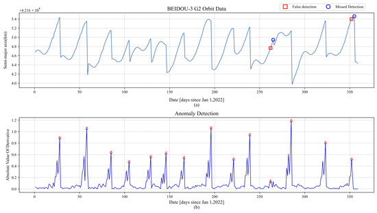
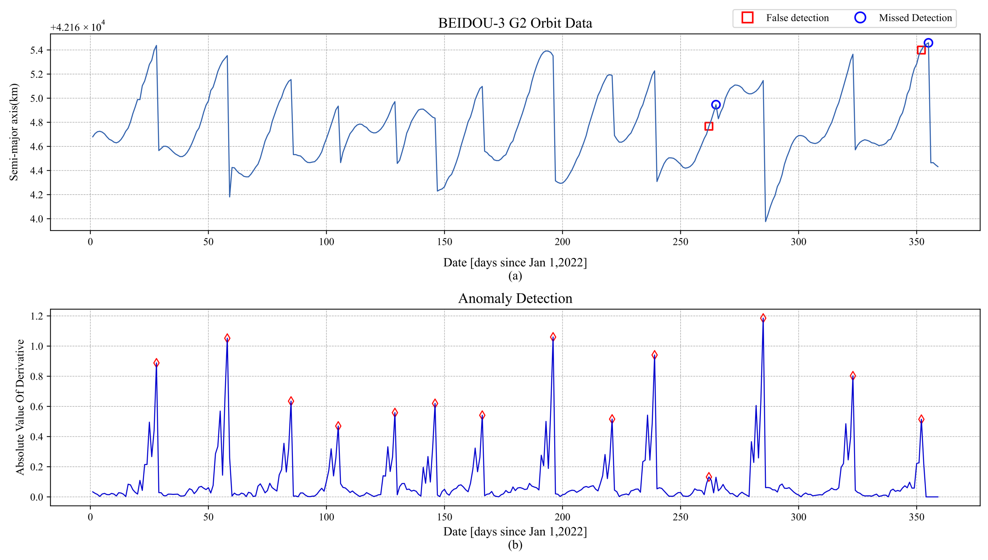
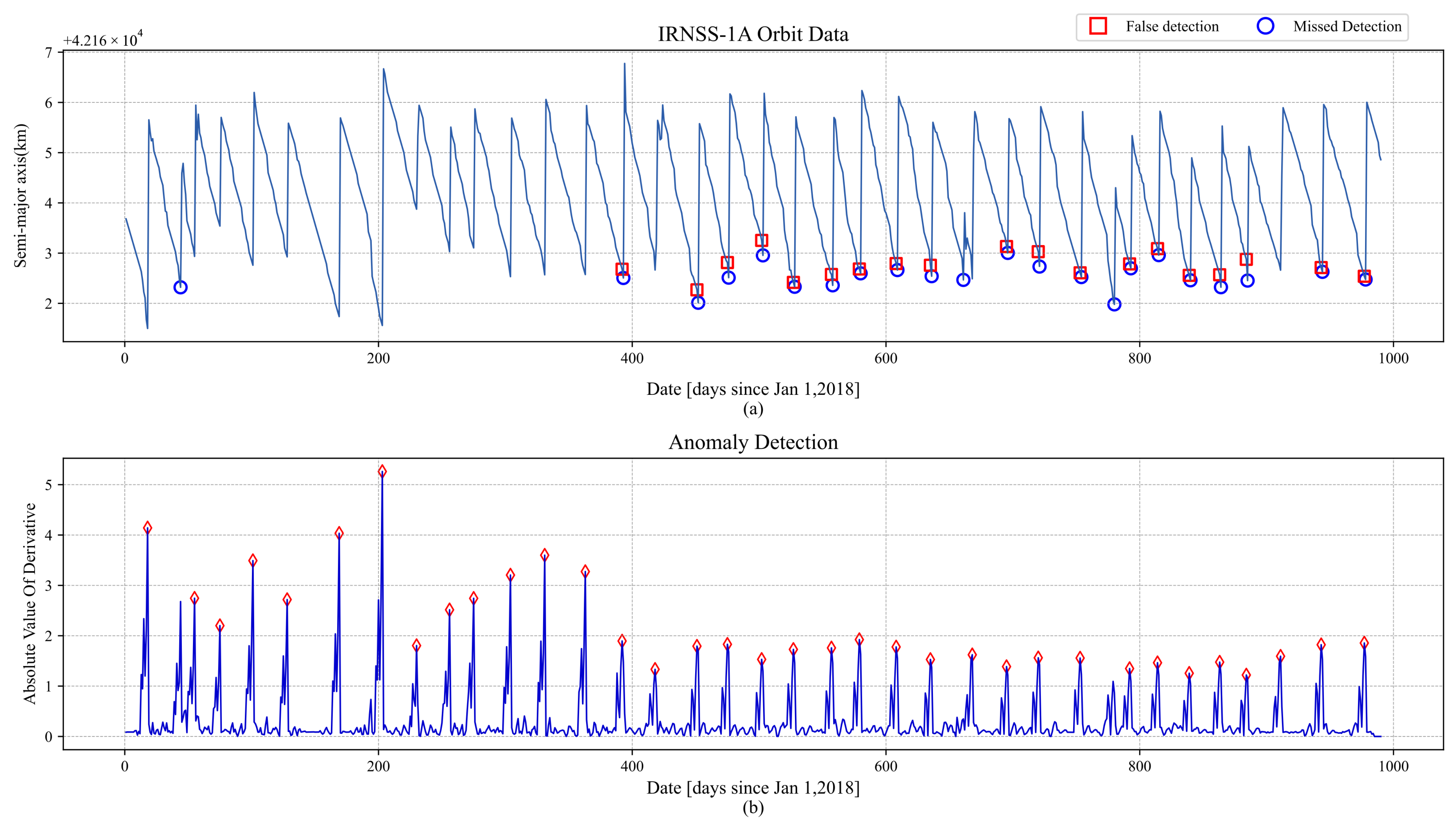
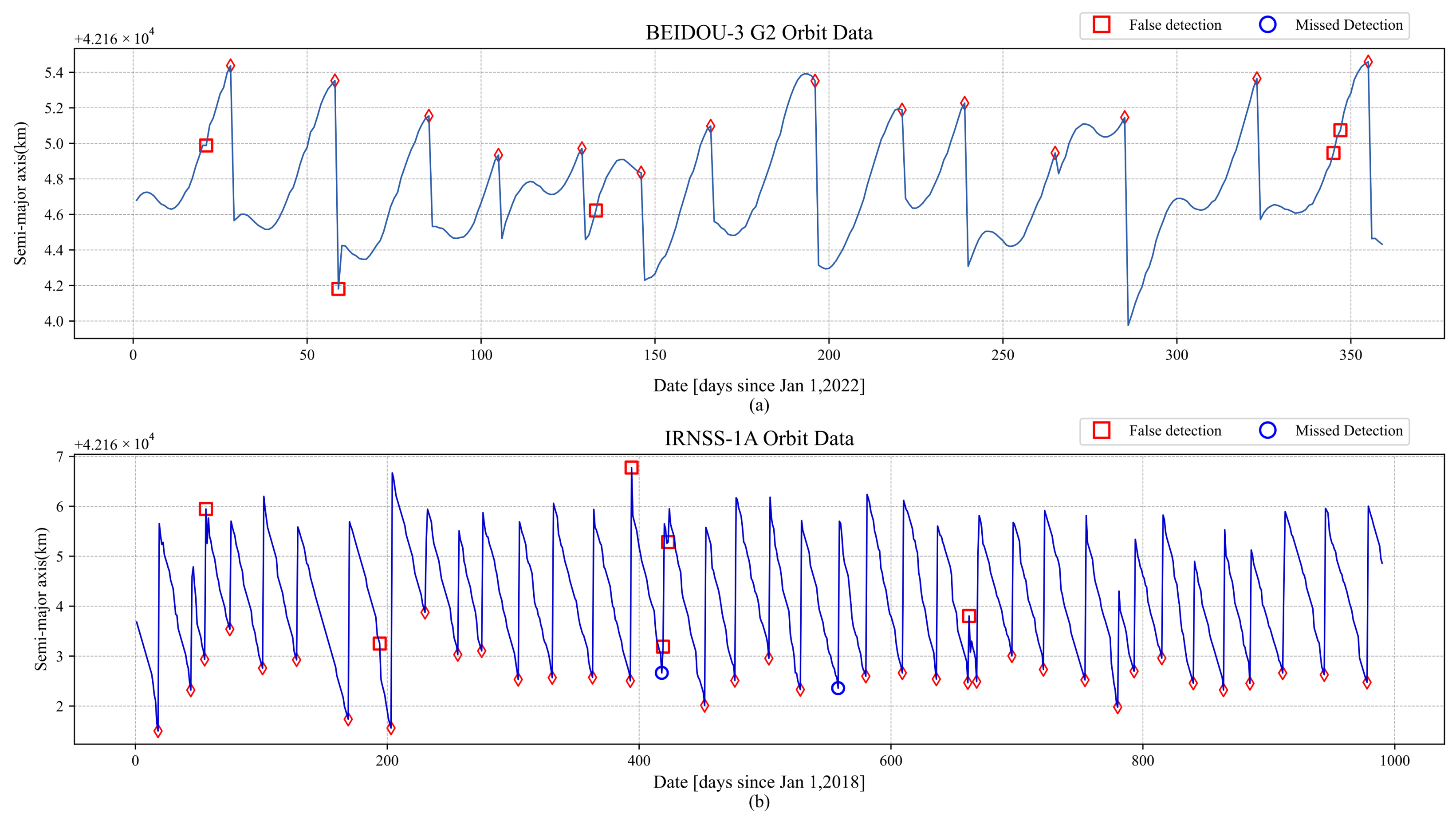
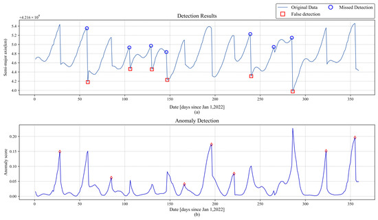
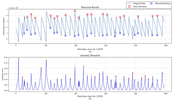
To provide a clearer visual comparison of the detection performance across the six methods, we have plotted their respective detection results from one experiment. Figure 6, Figure 7 and Figure 8 present the results from the traditional methods, while Figure 9, Figure 10, Figure 11, Figure 12, Figure 13, Figure 14, Figure 15 and Figure 16 illustrate the results from the deep learning methods. In these figures, red squares indicate false positives, and blue circles represent missed detections.
Figure 6.
BEIDOU-3 G2 satellite MWCF detection results: (a) false detection and missed detection annotations for the MWCF method; (b) the derivative sequence corresponding to the orbit, with red diamonds indicating the respective peaks.
Figure 7.
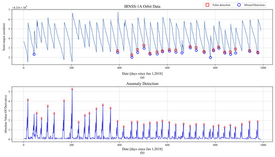
IRNSS-1A satellite MWCF detection results: (a) false detection and missed detection annotations for the IRNSS-1A satellite MWCF detection results; (b) the derivative sequence corresponding to the orbit, with red diamonds indicating the respective peaks.
Figure 8.
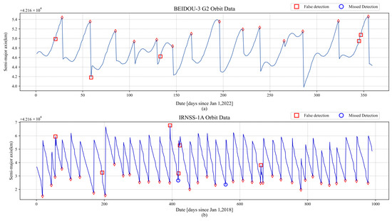
SACM detection results: (a) SACM detection results on the BEIDOU-3 G2 satellite, with red diamonds for correct detections; (b) SACM detection results on the IRNSS-1A satellite, with red diamonds for correct detections.
Figure 9.
VAE detection results for BEIDOU-3 G2: (a) the comparison between the original orbit and the VAE reconstruction result; (b) the absolute value of the residual between the original orbit and the VAE reconstruction result, with red diamonds indicating the respective peaks.
Figure 10.
VAE detection results for IRNSS-1A: (a) Comparison between the original orbit and the VAE reconstruction result for IRNSS-1A; (b) Absolute value of the residual between the original orbit and the VAE reconstruction result for IRNSS-1A, with red diamonds indicating the respective peaks.
Figure 11.
USAD detection results for BEIDOU-3 G2: (a) False detection and missed detection annotations for the USAD model. (b) The anomaly scores obtained by the USAD model, with diamonds indicating correctly detected points.
Figure 12.
USAD detection results for IRNSS-1A: (a) False detection and missed detection annotations for the USAD detection results on IRNSS-1A. (b) The anomaly scores obtained by the USAD model on IRNSS-1A, with red diamonds indicating correctly detected points.
Figure 13.
Anomaly-Transformer detection results for BEIDOU-3 G2: (a) the comparison between the original orbit and the Anomaly-Transformer reconstruction result; (b) the absolute value of the residual between the original orbit and the Anomaly-Transformer reconstruction result, with red diamonds indicating correctly detected points.
Figure 14.
Anomaly-Transformer detection results for IRNSS-1A: (a) the comparison between the original orbit and the Anomaly-Transformer reconstruction result for IRNSS-1A; (b) the absolute value of the residual between the original orbit and the Anomaly-Transformer reconstruction result for IRNSS-1A, with red diamonds indicating correctly detected points.
Figure 15.
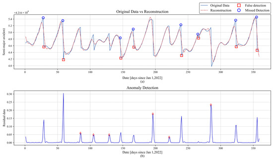
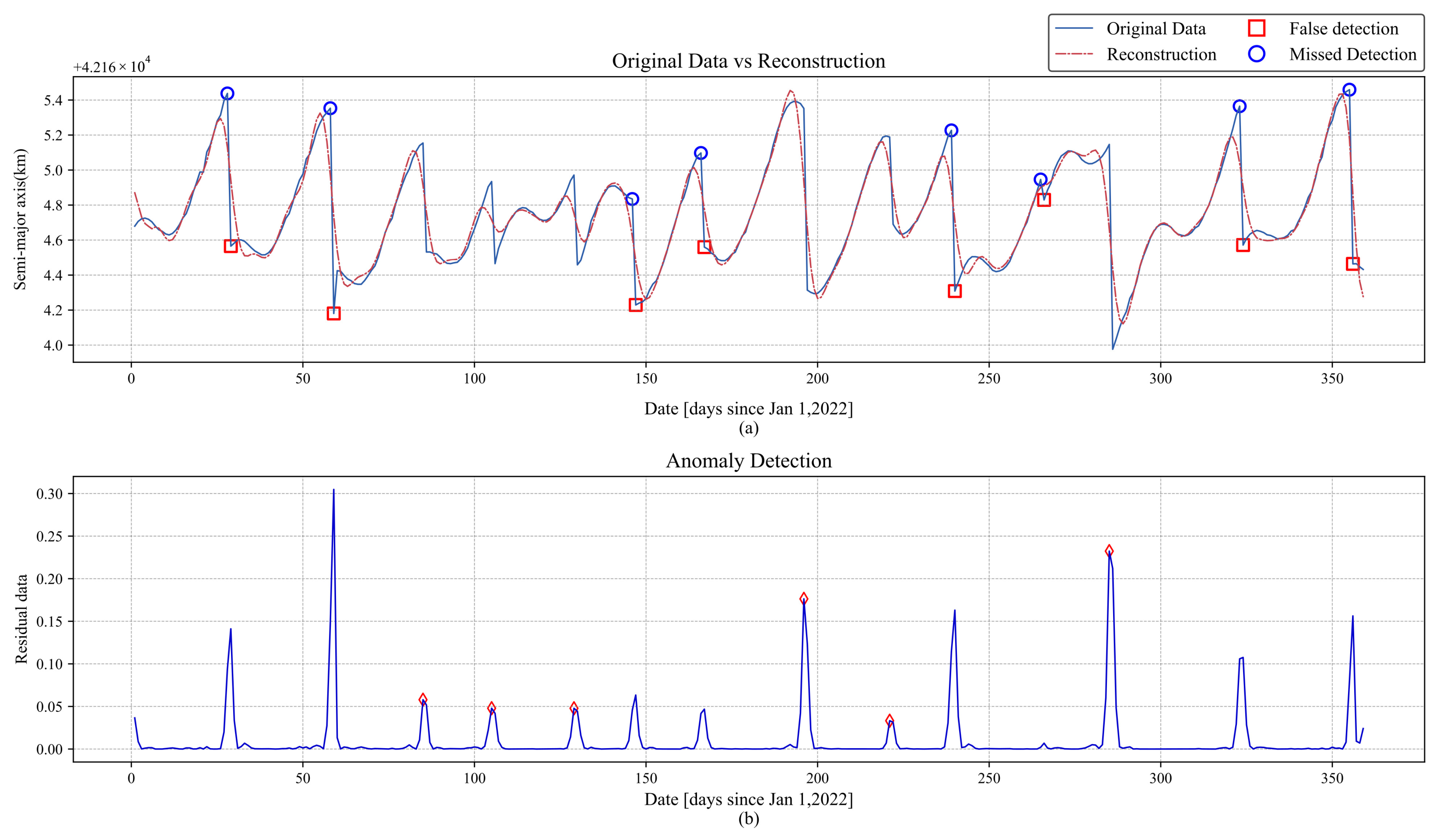
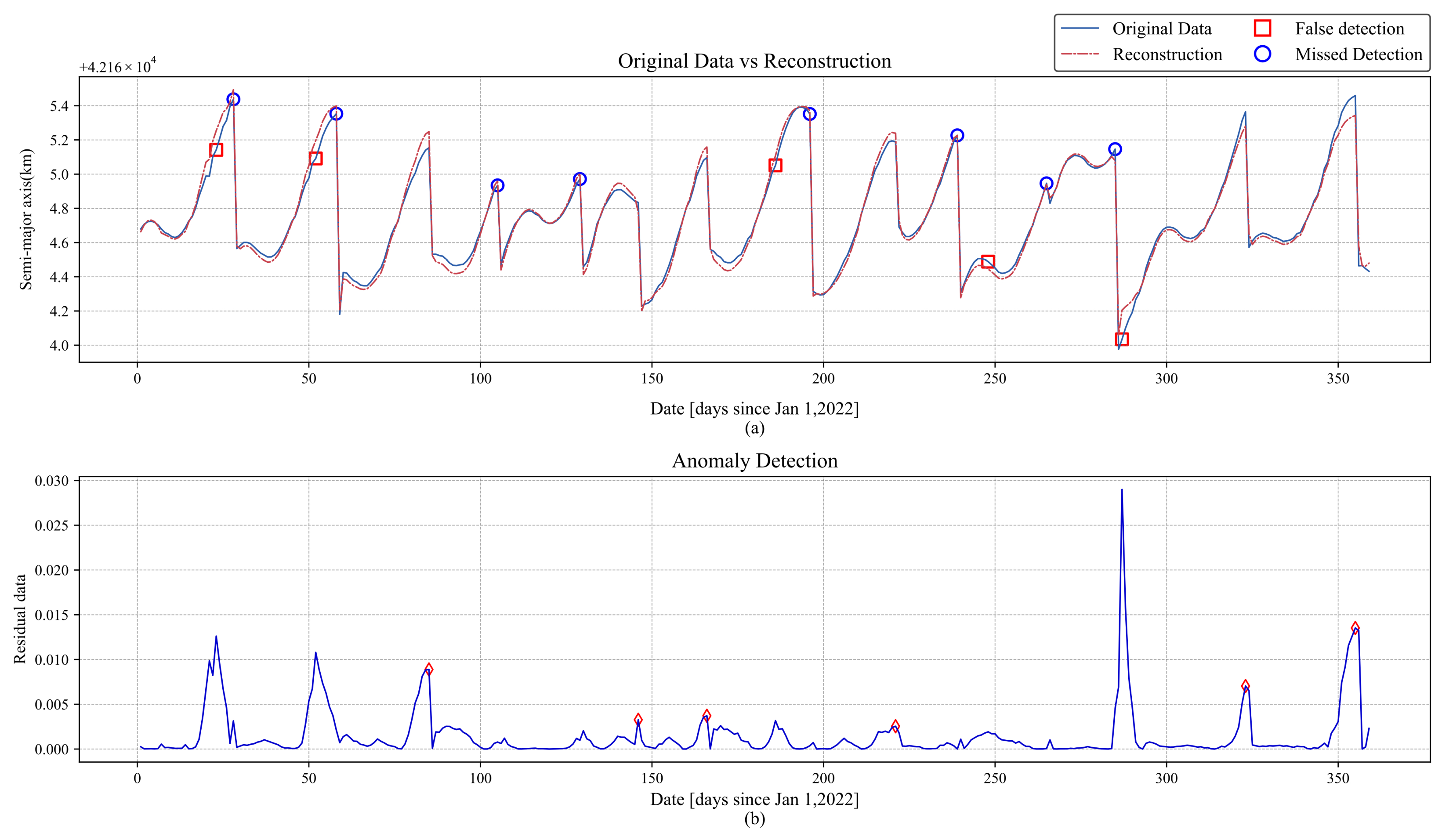
Peak-AAE detection results for BEIDOU-3 G2: (a) the comparison between the original orbit and the Peak-AAE reconstruction result; (b) the absolute value of the residual between the original orbit and the Peak-AAE reconstruction result, with diamonds indicating residual peaks.
Figure 16.
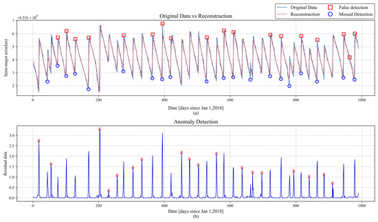
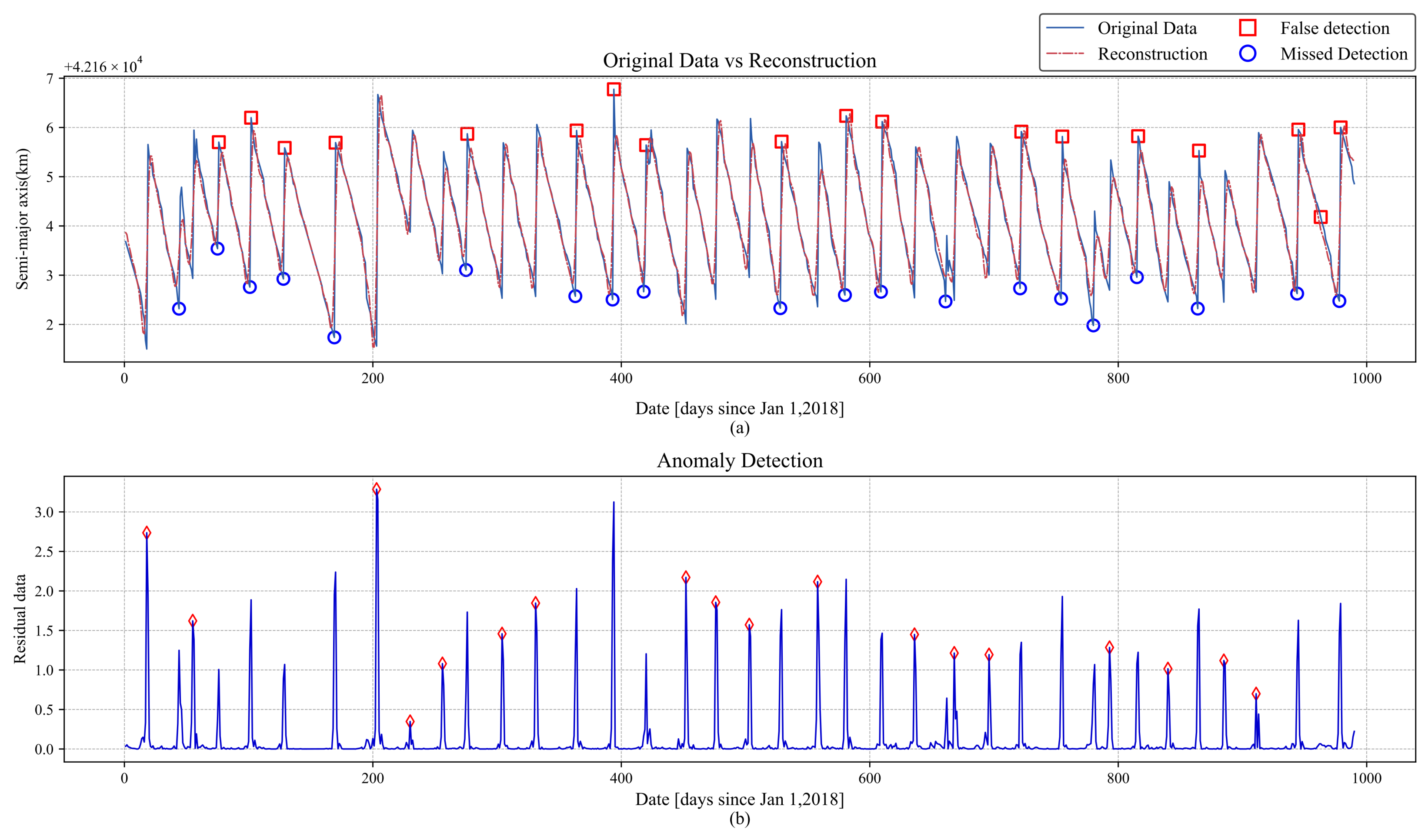
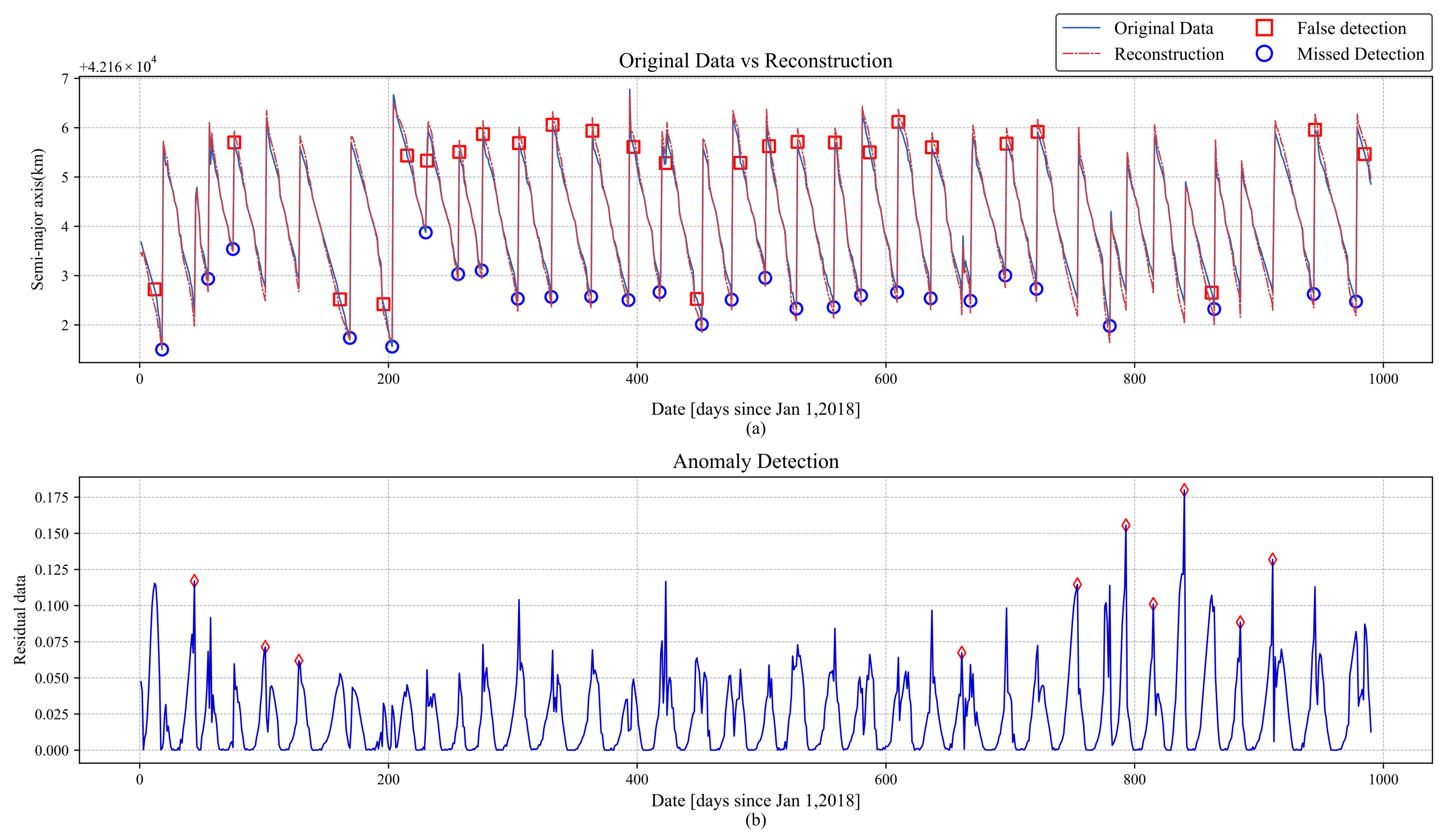
Peak-AAE detection results for IRNSS-1A: (a) the comparison between the original orbit and the Peak-AAE reconstruction result for IRNSS-1A; (b) the absolute value of the residual between the original orbit and the Peak-AAE reconstruction result for IRNSS-1A, with diamonds indicating residual peaks.
In the detection of BEIDOU-3 G2, as shown in Figure 6a, MWCF had two missed detections and one false detection. The missed detections occurred on day 265 and day 355. In the corresponding derivative sequence, as shown in Figure 6b, day 261 and day 351 were falsely detected as anomalies. This indicates that MWCF advanced the position of the missed anomaly points, which may be due to the fact that the MWCF method identifies anomalies based on the derivative.
In the detection of IRNSS-1A, as shown in Figure 7a, there were three independent missed detections, occurring on day 44, day 661, and day 780. In the corresponding derivative sequence, as shown in Figure 7b, it can be seen that the missed detections on day 44 and day 780 were caused by the AMPD algorithm, which failed to detect the anomalies, while MWCF did identify them. However, the missed detection on day 661 was due to the fact that two anomalies were too close together, and MWCF failed to detect the anomaly. The remaining missed detections and false detections occurred in pairs: the anomalies on days 393, 452–636, 696–754, and 793–885, as well as the individual anomalies on days 944 and 978. These missed detections were caused by false detections from the MWCF method, where the missed anomaly points were incorrectly identified at other locations, leading to false detections.
In Figure 8, the red diamonds represent the correctly detected anomaly points. The detection results of BEIDOU-3 G2 are shown in Figure 8a. It can be seen that the SACM detected all the orbital abnormal points, but there were many false detections. This may be because the threshold set by the SACM is too small, leading to points with significant variations being identified as anomalies.
The detection results for IRNSS-1A are shown in Figure 8b. There were two missed detections and six false detections. The missed detection points occurred on day 418 and day 558. The missed detection on day 418 was due to a small change in the orbital maneuver, while the cause of the missed detection on day 558 remains unclear. The false detection points occurred on days 56, 194, 394, 419, 423, and 662. Among these, the false detections on days 194 and 419 were caused by significant orbital changes during normal satellite operation, while the remaining false detections are most likely caused by the excessively low threshold set in the SACM.
The reconstruction results of VAE are shown in Figure 9 and Figure 10, with red diamonds representing correctly detected anomaly points. In the detection results for BEIDOU-3 G2, missed detection points and false positive points correspond to each other: shifting the false positive points one position forward yields the missed detection points, thereby avoiding missed detections. This confirms the statement in the introduction that “Common reconstruction models (VAE, GAN, transformer) cannot distinguish between the onset and end phases of orbit anomalies and randomly identify either as anomalies, leading to false detections.”
The situation with IRNSS-1A is similar. Aside from the missed detection points 44, 661, and 780, and the false positive point 963, all other missed detection points can be obtained by shifting the corresponding false positive points one position forward. These three specific missed detection points primarily occurred due to their proximity to other anomaly points, which the AMPD algorithm failed to identify separately, while the false positive point resulted from poor reconstruction performance by the VAE model.
The detection results of USAD are shown in Figure 11 and Figure 12. Its performance is consistent with that of VAE, where shifting the false positives one position forward yields most of the missed detections, with only a few exceptions (point 265 for BEIDOU-3 G2, and points 55, 661, and 793 for IRNSS-1A). Among these, point 265 for BEIDOU and point 661 for IRNSS were too close to other anomaly points, which the AMPD algorithm failed to distinguish, leading to the missed detections. The missed detections for IRNSS (points 55 and 793), however, were caused by the USAD model itself, as their corresponding anomaly scores did not exhibit peak values.
The reconstruction results of Anomaly-Transformer are shown in Figure 13 and Figure 14. Compared to VAE and USAD, the detection results of the Transformer are more complex. While most missed detections can still be obtained by shifting false positives forward, some missed detections do not follow this pattern. For BEIDOU-3 G2, missed detection points (28, 58, 196) require shifting the corresponding false positives (23, 52, 186) backward to obtain them. Similarly, for IRNSS-1A, missed detection points (18, 169, 203, 452, 864) also exhibit this behavior. One possible explanation is that the Minimax strategy makes the model overly sensitive to anomalies, causing it to identify deviations before the actual anomaly as anomalies, although the exact reason remains unclear. As for the remaining missed detections, except for point 780 in IRNSS-1A, which is attributed to AMPD, all others are caused by the model itself.
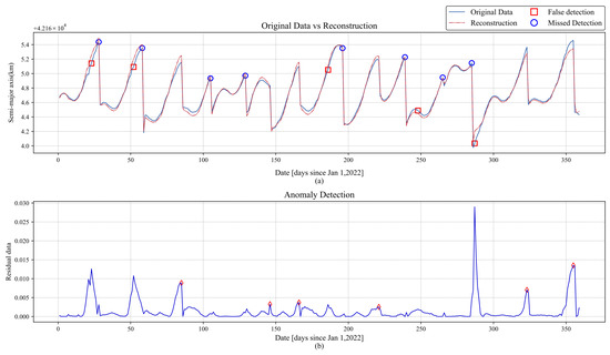
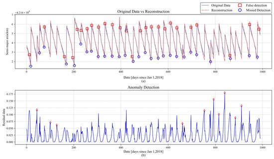
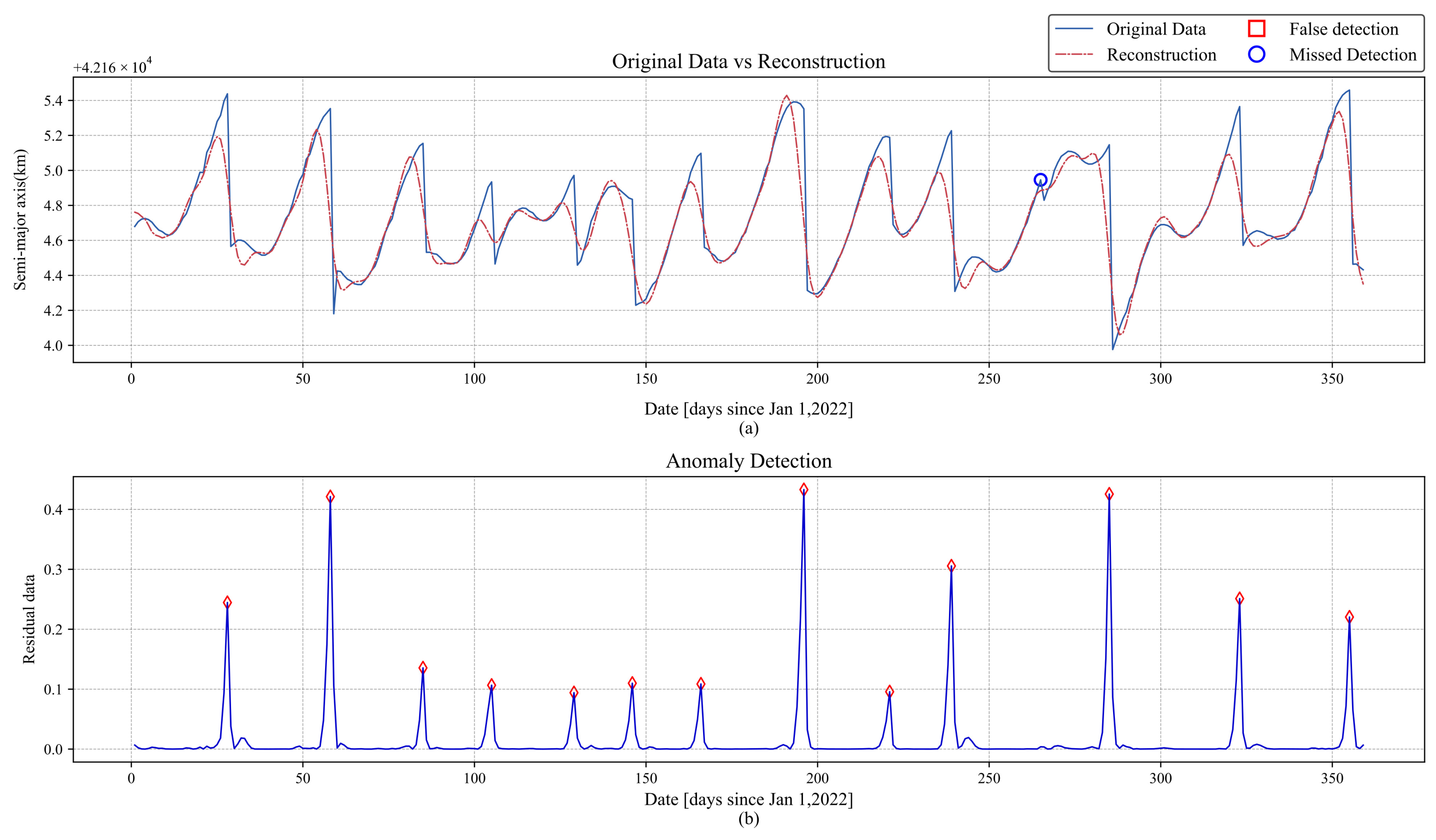
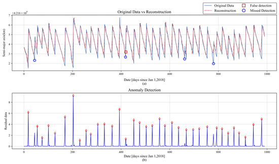
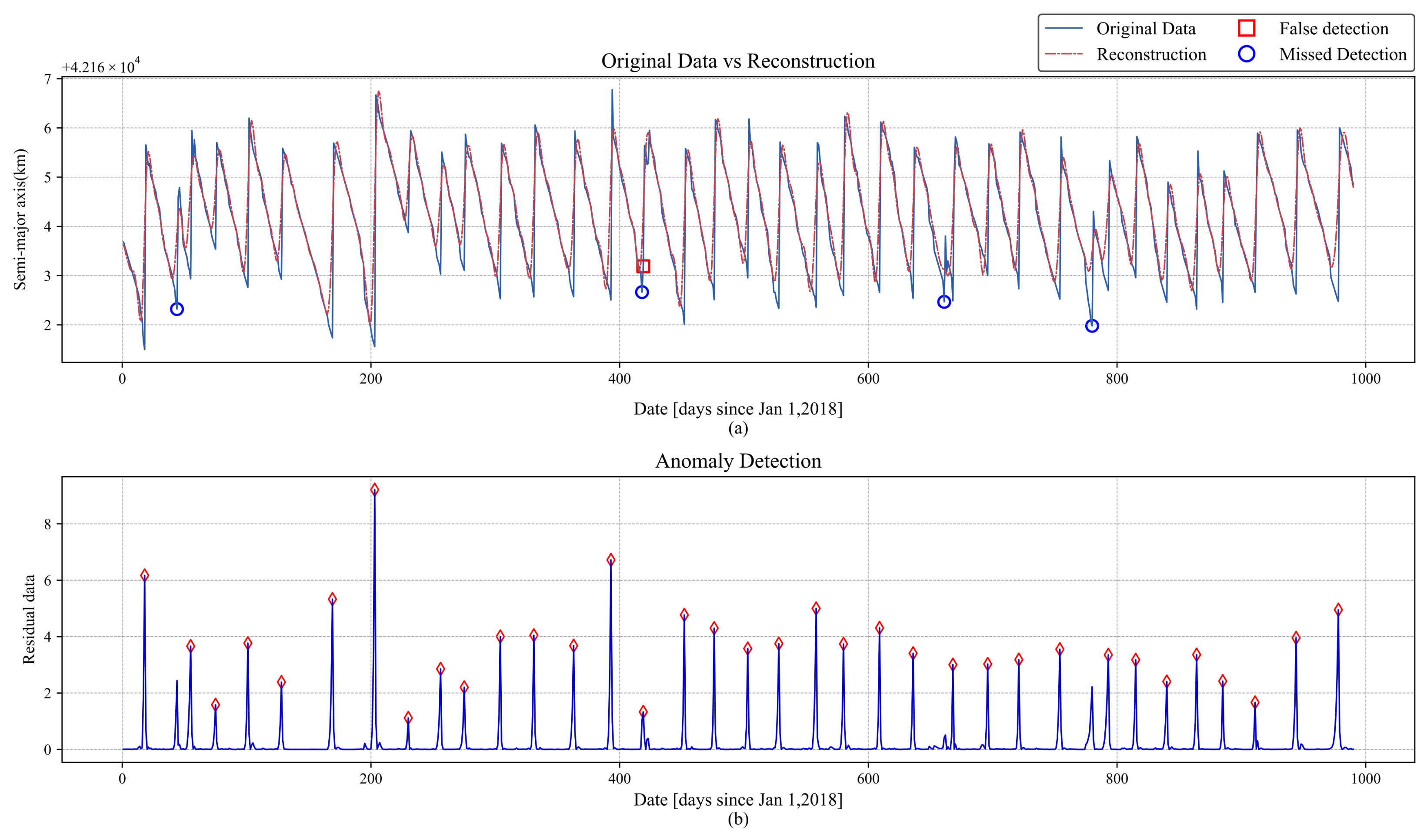
The reconstruction results of the Peak-AAE are shown in Figure 15a and Figure 16a, with the corresponding residual sequences presented in Figure 15b and Figure 16b. The blue solid line represents the true semi-major axis data, the red dashed line indicates the reconstruction results, and the red diamonds denote correctly identified anomalies.
As shown in Figure 15a, the proposed method exhibited one miss for the BEIDOU-3 G2 satellite. The missed detection occurred on day 265. This is primarily because the orbital maneuver on day 265 had a relatively small magnitude, causing the model to fail to detect it.
For the IRNSS-1A satellite, the proposed method yielded one false detection and four misses, as shown in Figure 16a. The false detection occurred on day 419, and the misses occurred on days 44, 418, 661, and 780. As evident from the residual sequence in Figure 16b, the residual values on days 44 and 780 can successfully identify anomalies. The missed detections are primarily caused by the failure of the AMPD algorithm to recognize these anomalies. The missed detections on days 418 and 661, as well as the false positive on day 419, are attributed to the Peak-AAE model. In the residual sequence constructed by the Peak-AAE, the residual value on day 419 is higher than that on day 418, while the residual value on day 661 is too small, leading to the occurrence of false positives.
3.4. Ablation Study
To validate the effectiveness of the proposed improvements, we conducted five independent ablation experiments comparing the original AAE model and the AMPD algorithm. The comparative models are as follows: AAE-AMPD, Peak-AAE-AMPD, AAE-AMPD*, and Peak-AAE-AMPD*, where AMPD* denotes the modified version of the AMPD algorithm. The experimental results are shown in Table 6 and Table 7, and the corresponding t-distribution confidence intervals are provided in Appendix A (Table A3 and Table A4).
Table 6.
Results of ablation study on BEIDOU-3 G2.
Table 7.
Results of ablation study on IRNSS-1A.
The comparison of the first and second or third and fourth rows in Table 6 and Table 7 shows that, under the same detection algorithm, the Peak-AAE model achieves higher scores in three indicators compared to the original model. This indicates that the improved model can identify more anomalies and reduce false detections. Meanwhile, for AAE-AMPD, all metric means on the two satellites remained below 50%, which demonstrates that the original AAE model is not well suited for handling track anomaly detection.
Comparing the first and third rows, the precision of the improved AMPD algorithm decreases when the recall remains similar. This may be attributed to the AAE model generating a large number of false positives. The improved AMPD algorithm demonstrates stronger detection capabilities and identifies more false positives, which results in a decrease in precision. In comparison between the second and fourth rows, under the improved AAE model, the improved AMPD algorithm achieves higher scores across all other evaluation metrics, except for a decrease in precision on BEIDOU-3 G2, indicating better detection performance.
When comparing the second and third rows, it is evident that the improved AAE model outperforms the improved AMPD algorithm in terms of indicator scores. This suggests that the reconstruction capability of the model plays a crucial role in anomaly detection. Therefore, enhancing the model’s reconstruction ability is more critical than improving the accuracy of the detection algorithm itself.
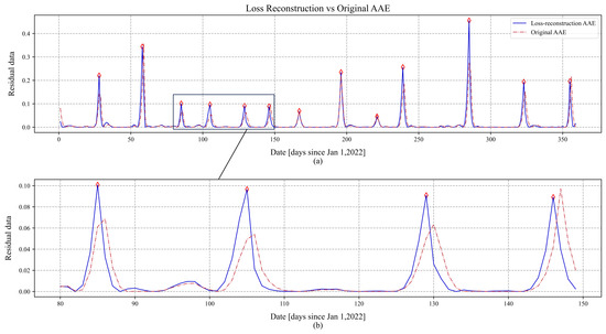
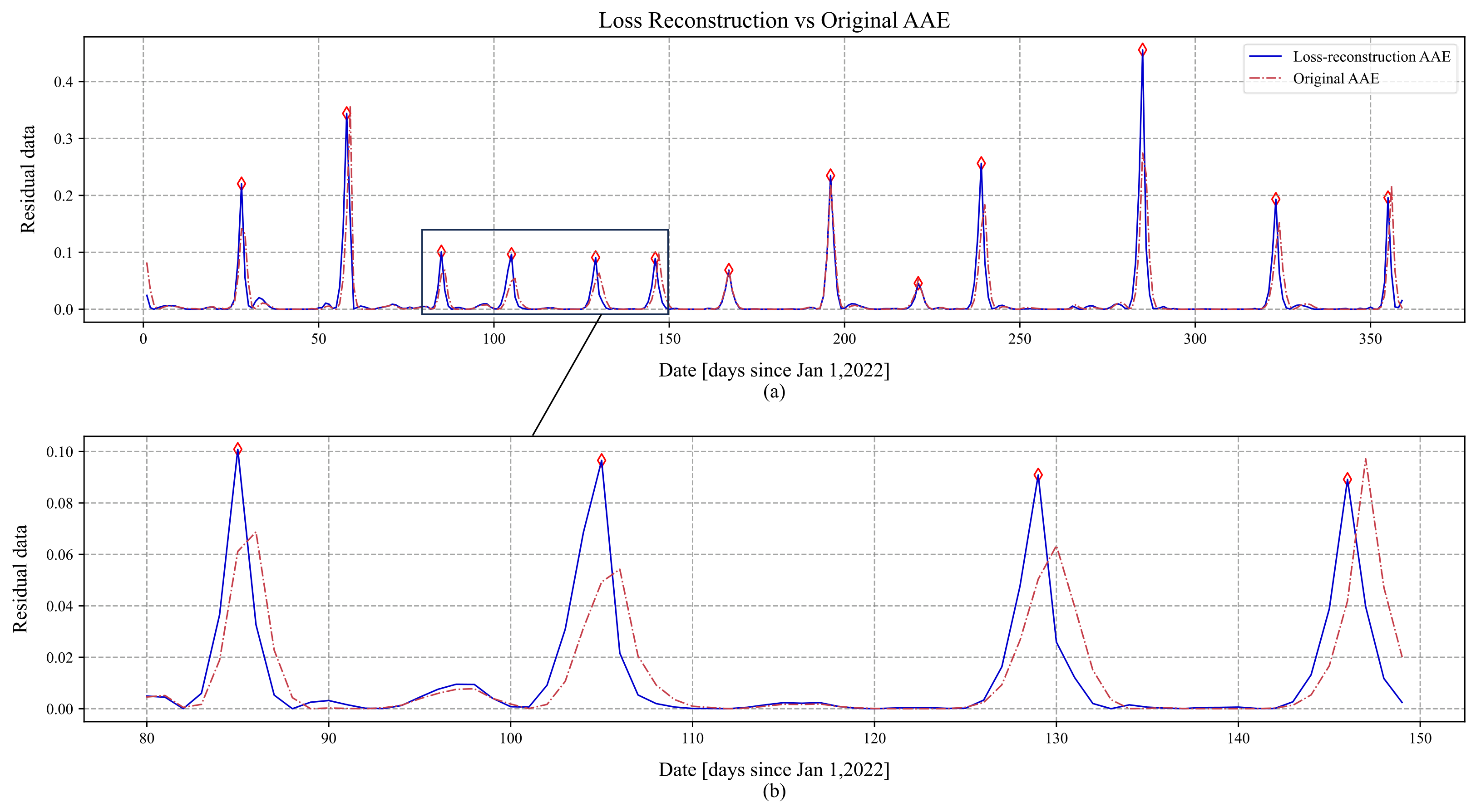
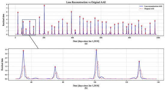
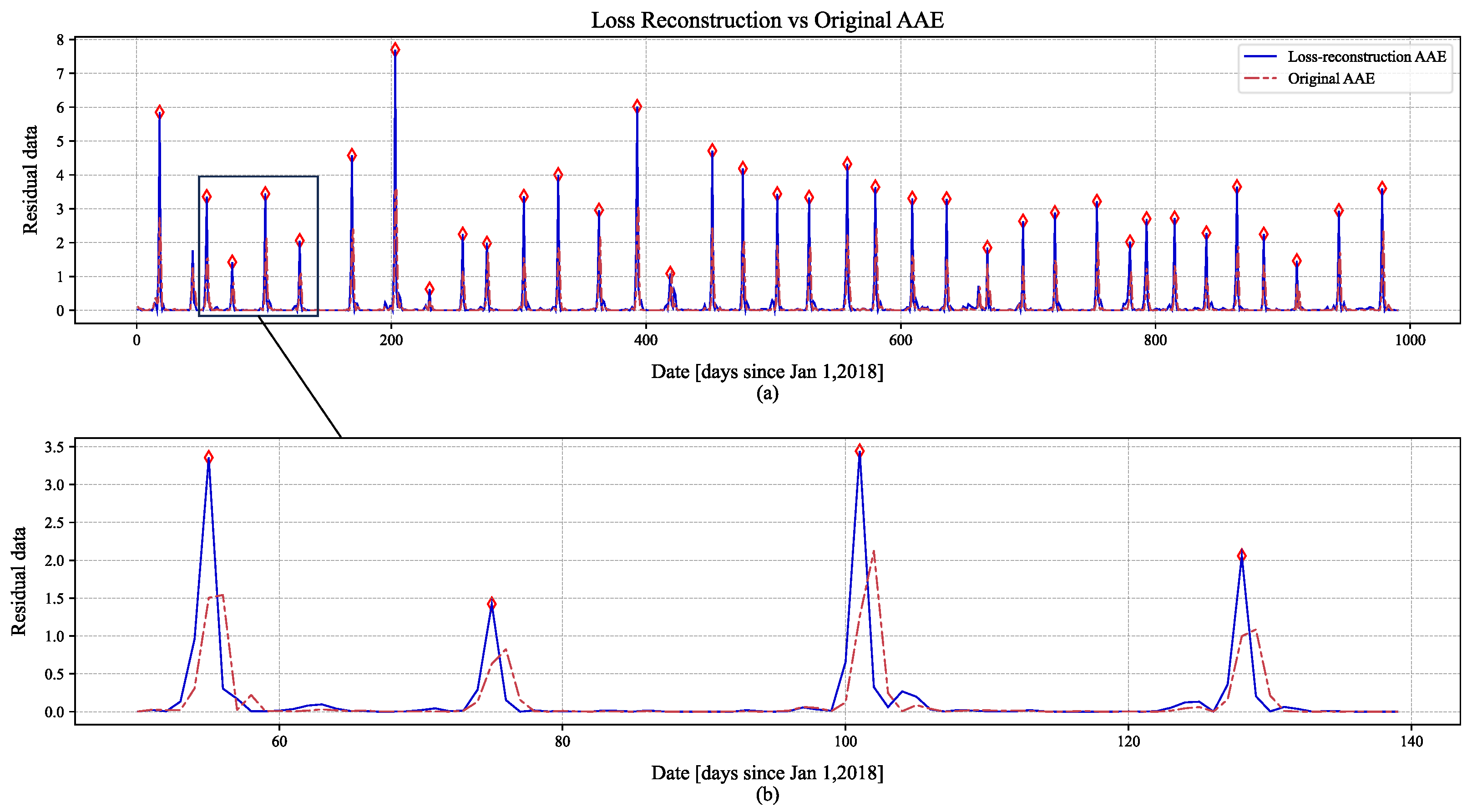
Figure 17 and Figure 18 provide a detailed comparison of the reconstruction capabilities between the Peak-AAE model and the original AAE model. The blue solid line represents the reconstruction results of the improved model, the red dashed line indicates the reconstruction results of the original AAE model, and red diamonds denote the locations of correctly identified anomalies. Figure 17a and Figure 18a display the residual plots obtained after reconstruction. Figure 17b and Figure 18b show the corresponding close-up views of the residual plots.
Figure 17.
BEIDOU-3 G2 reconstruction effect comparison graph: (a) Comparison of detection performance between Peak-AAE and Original AAE, with red diamonds indicating correctly detected points; (b) Enlarged local view of the comparison figure.
Figure 18.
IRNSS-1A reconstruction effect comparison graph: (a) Comparison of detection performance between Peak-AAE and Original AAE, with red diamonds indicating correctly detected points; (b) Enlarged local view of the comparison figure.
As evident from Figure 17b and Figure 18b, the Peak-AAE model accurately identifies the locations of anomaly points. In contrast, the original AAE model exhibits a lag in anomaly detection relative to the actual occurrence times. This lag is attributed to the original model’s inability to distinguish between the onset and conclusion phases of orbital anomalies. Furthermore, the identification features constructed by the Peak-AAE model are more readily discernible, characterized by significantly larger residual values at anomaly points compared to those at normal points. This distinct difference enables the detection algorithm to readily identify anomalies.
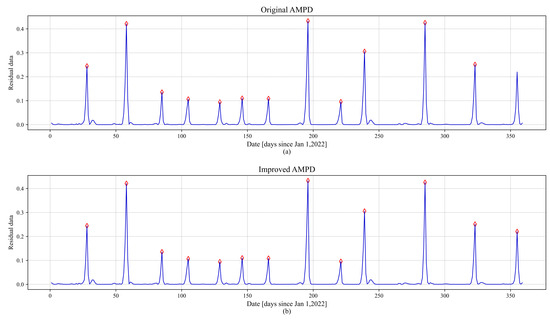
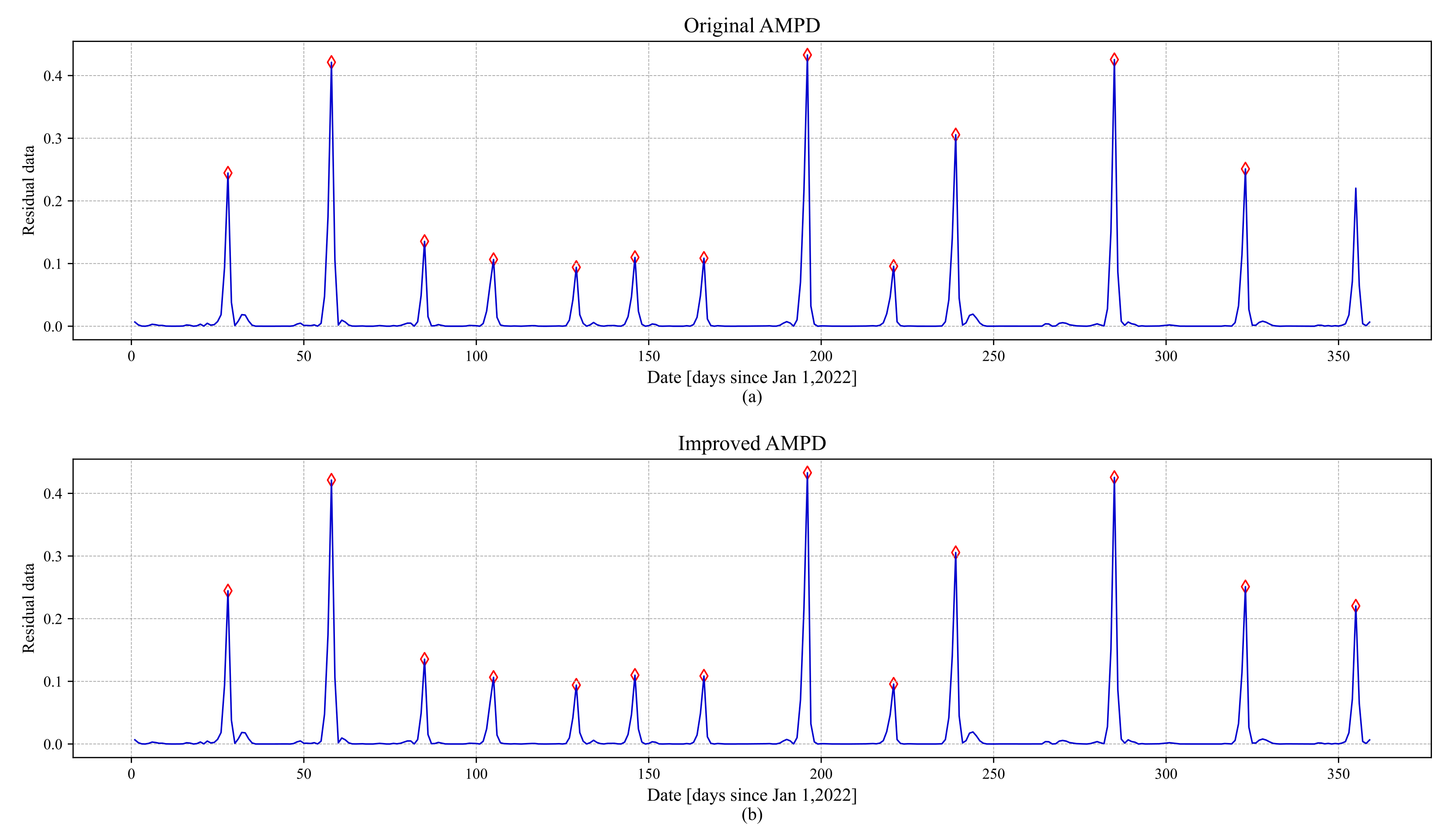
Figure 19 presents the detection performance of the two AMPD algorithms on the BEIDOU-3 G2 satellite. Figure 19a shows the results obtained with the vanilla AMPD algorithm, while Figure 19b displays those from the improved AMPD algorithm.
Figure 19.
Comparison of the AMPD effect: (a) Detection results of the original AMPD method, with red diamonds indicating correctly detected points; (b) Detection results of the improved AMPD method, with red diamonds indicating correctly detected points.
It can be observed that the vanilla AMPD algorithm failed to detect the anomaly on day 355. This failure is due to the algorithm’s constraint of limiting indices to the range during traversal—where N denotes the data length and k represents the optimal scale—implemented to prevent index out-of-bounds errors. By applying edge padding to both ends of the original data, the improved AMPD algorithm effectively mitigates this issue of missed detections at the data boundaries.
4. Edge Model Deployment
4.1. Overall Framework
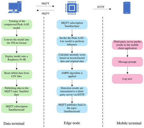
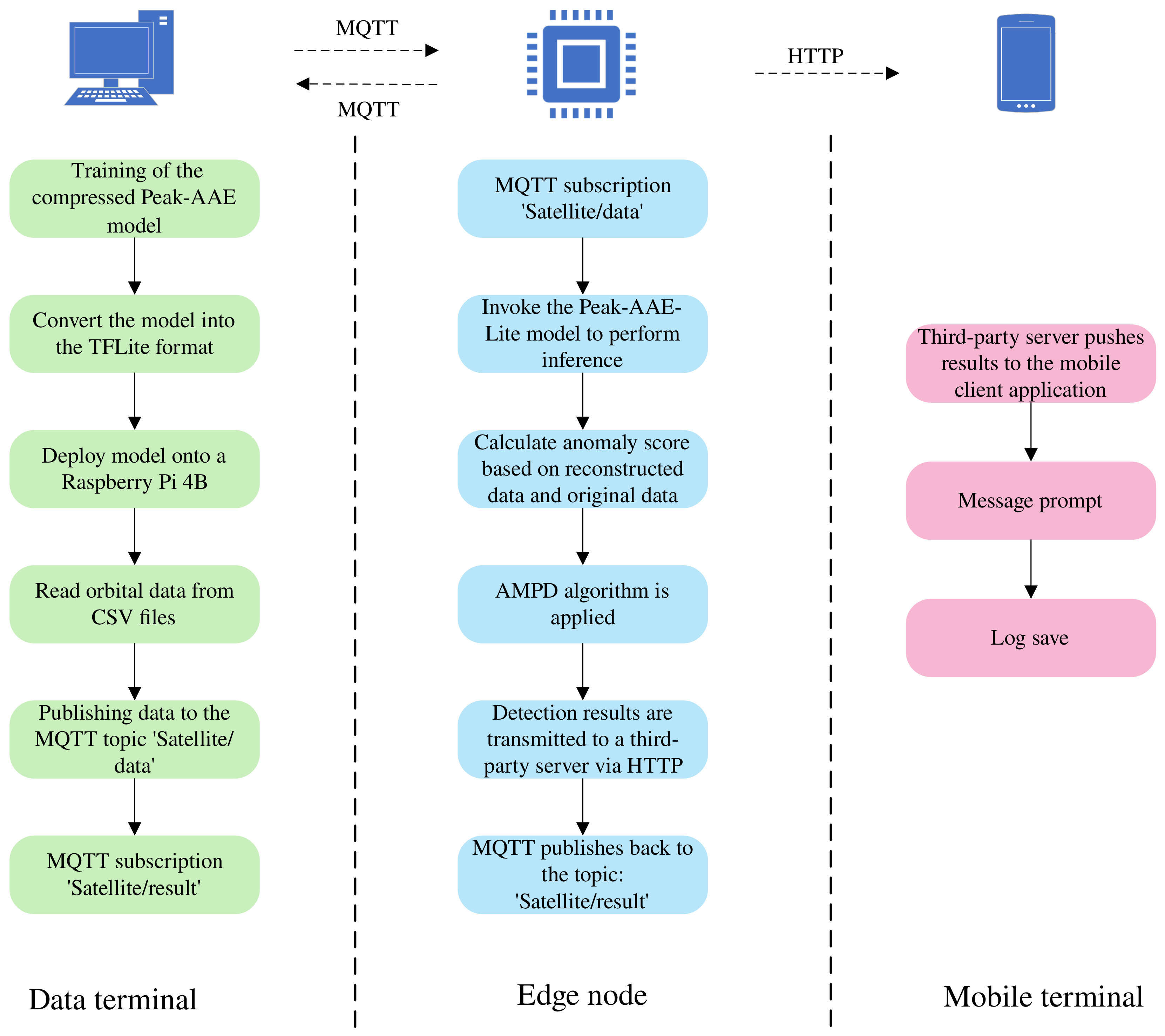
To validate the deployability of the proposed method in practical engineering scenarios, we conducted ground simulation verification on a Raspberry Pi and constructed an orbital anomaly detection system comprising a data terminal, edge nodes, and a mobile terminal. The overall architecture is illustrated in Figure 20, and the detailed software and hardware environments are provided in Table 8. This system adopts a collaborative operational model in which the data terminal is responsible for model training and distribution, the edge nodes perform detection and decision-making tasks, and the mobile terminal handles alert notifications and information logging. This approach extends orbital anomaly detection from purely algorithmic research into a fully executable engineering framework.
Figure 20.
Orbit anomaly detection system structure diagram.
Table 8.
Edge device deployment parameters.
As depicted in Figure 20, the data terminal undertakes the offline training of the compressed Peak-AAE model. Once training is complete, the terminal converts the model into the TFLite floating-point format and deploys it onto a Raspberry Pi 4B. Simultaneously, the data terminal reads orbital data from CSV files, extracts the semi-major axis sequence, and publishes it under the predefined satellite/data topic, thereby providing a continuous input stream for the edge nodes.
The edge node serves as the primary execution unit of the system. Upon subscribing to orbital data via MQTT, the node invokes the Peak-AAE-Lite model to perform inference on the input sequence, yielding reconstructed data. The squared error between the original and reconstructed data is employed as the anomaly score. To mitigate the influence of manual threshold selection, the AMPD algorithm is applied to the anomaly score sequence for peak detection. The detection results are published back to the satellite/result topic for monitoring and debugging purposes at the control terminal, and are concurrently transmitted to a third-party server via an HTTP interface, providing an entry point for mobile alert notifications.
The mobile terminal is primarily responsible for result presentation and human–machine interaction. Upon receiving the detection results forwarded by the edge node, the third-party server pushes critical information—such as anomaly timestamps, satellite identifiers, and anomaly scores—to the mobile client application, while simultaneously logging the data for subsequent anomaly tracing and manual verification. Collectively, the system establishes a complete processing pipeline encompassing orbital data acquisition, anomaly identification, and result visualization.
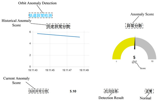
Figure 21 presents the user interface, which is built with Node-RED. The interface itself is in Chinese, but English annotations are provided at the corresponding positions. The project title is Orbit Anomaly Detection. Directly beneath it, the historical anomaly score is shown as a line chart that displays historical values. To the right and below, the current anomaly score is presented in two different formats: on the right, it is indicated by a gauge, while below, the numerical value is given directly. Finally, the detection result outputs the satellite’s operating status label—either normal or abnormal.
Figure 21.
User interface.
4.2. Model Compression
During edge deployment, the model size directly determines both storage overhead and response latency. To address this, we performed lightweight structural pruning on the network architecture while preserving the fundamental detection mechanism of Peak-AAE, yielding the compressed variant Peak-AAE-Lite. A comparison of parameter counts between the two models is presented in Table 9, and the performance comparison is shown in Table 10. The inference test was conducted 200 times, the throughput test lasted 10 s, and the memory test was performed over 50 inferences. The model input window size was set to 24. This was primarily to adapt to the broadcast ephemeris data, as its update frequency is generally once per hour, resulting in 24 data records per day.
Table 9.
Comparison of model parameters.
Table 10.
Comparison of inference performance.
As shown in Table 9, after lightweight compression, the total number of model parameters is reduced from approximately 28.5 k to about 9.3 k, corresponding to a compression ratio of approximately 67.4%, which significantly lowers model storage and transmission overhead. In Table 10, from the perspective of inference efficiency, the average inference latency of the compressed model drops from 0.13 ms to 0.08 ms, the P95 latency drops from 0.26 ms to 0.11 ms, and the throughput increases from 10,793.93 inferences per second to 13,688.56 inferences per second, indicating that model compression not only reduces model scale but also brings higher real-time inference capability and more stable response performance. It should be noted that the peak inference memory is primarily affected by the TensorFlow Lite runtime, delegates, and the allocation of input/output tensors; therefore, the difference before and after compression is less pronounced than the changes in model parameter size and inference latency. Nevertheless, considering model size, loading memory, and inference efficiency together, the compressed model offers clear advantages in resource-constrained environments and can better satisfy the requirements of lightweight design and real-time performance for edge deployment.
4.3. Detection Performance Analysis
In addition to resource considerations, edge deployment also imposes stringent requirements on detection accuracy. We conducted five independent repeated experiments comparing the detection results of Peak-AAE and Peak-AAE-Lite on two GEO satellites. The results are shown in Table 11 and Table 12, and the corresponding t-distribution confidence intervals are provided in Appendix A (Table A5 and Table A6).
Table 11.
Comparison of evaluation metrics on BEIDOU-3 G2.
Table 12.
Comparison of evaluation metrics on IRNSS-1A.
As shown in Table 11 and Table 12, after model compression, the detection metrics have declined to some extent, but the overall decrease is small, and the compressed model still maintains relatively high detection performance. On the BEIDOU-3 G2 dataset, the recall of the compressed model remains consistent with the original model, both at 94.29%, indicating that model compression does not impair the ability to detect real maneuver events. Precision decreases from 94.57% to 88.32%, a drop of 6.25 percentage points; the F1-score decreases from 94.33% to 91.12%, a drop of only 3.21 percentage points. This shows that although the compressed model has a slight decline in false alarm control, its overall detection performance remains close to that of the original model. In particular, with recall unchanged, the compressed model can still effectively identify the vast majority of orbital maneuver events. On the IRNSS-1A dataset, the precision, recall, and F1-score of the compressed model are 85.32%, 79.47%, and 82.29%, respectively, with decreases of 4.68, 5.27, and 4.99 percentage points compared to the original model. Despite some performance degradation, the F1-score of the compressed model remains above 80%, demonstrating its relatively stable detection capability on another satellite dataset.
5. Conclusions and Discussion
This paper addresses the challenge of orbit anomaly detection by proposing an intelligent method that integrates a Peak Adversarial Autoencoder (Peak-AAE) with the Automatic Multi-Scale Peak Detection (AMPD) algorithm. Compared with traditional approaches, the proposed method eliminates the need for manual feature engineering, and a detection function without hyperparameters was selected. The methodology consists of three sequential steps: (1) reconstructing historical semi-major axis data using the Peak-AAE, (2) calculating the squared differences between the reconstructed and original data to produce residuals, and (3) performing anomaly detection on the residual sequence using the AMPD algorithm. Experimental validation on the BEIDOU-3 G2 and IRNSS-1A satellites demonstrates the superiority of the proposed method over traditional techniques. Furthermore, ablation studies comparing the vanilla AAE and the original AMPD algorithm confirm the effectiveness of the proposed modifications. Finally, the compressed Peak-AAE model was deployed on a Raspberry Pi for ground simulation verification, and an orbital anomaly detection system was designed accordingly, confirming the feasibility of practical model deployment.
The method described in this paper has currently been validated as effective only in the GEO scenario; however, from the dynamical perspective, the core mechanism of the method (SGP4 residual reconstruction) is independent of orbit type and can theoretically be extended to low Earth orbit (LEO), medium Earth orbit (MEO), and highly elliptical orbit (HEO).
Author Contributions
The experimental part of the paper was completed by Y.G.; X.Y. wrote the manuscript; B.W. and B.L. provided valuable comments on the paper revision; all authors reviewed the manuscript. All authors have read and agreed to the published version of the manuscript.
Funding
This work was supported by the Key Research and Development Program of Shandong Province, China, under Grant No. 2026CXPT113 for the project “Basic Research on Continuous Behavior Modeling and Cognitive Inference of Dynamic Targets Based on 3D Mesh Segmentation”.
Institutional Review Board Statement
Not applicable.
Informed Consent Statement
Not applicable for studies not involving humans.
Data Availability Statement
All satellite data are from Space-Track and can be accessed via the following link: https://www.space-track.org/.
Conflicts of Interest
The authors declare no conflicts of interest.
Abbreviations
The following abbreviations are used in this manuscript:
| TLE | Two-Line Element |
| AE | Autoencoder |
| AAE | Adversarial Autoencoder |
| GANs | Generative Adversarial Networks |
| NORAD | North American Aerospace Defense Command |
| MLPs | Multi-Layer Perceptrons |
| Peak-AAE | Peak Adversarial Autoencoder |
| AMPD | Automatic Multi-Scale Peak Detection |
| GEO | Geostationary Earth Orbit |
| BCELoss | Binary Cross-Entropy Loss |
| DOY | Day-Of-Year |
| MWCF | Moving-Window Curve Fitting |
| SACM | Semi-Major Axis Change Method |
| VAE | Variational Autoencoder |
| USAD | Unsupervised Anomaly Detection on Multivariate Time Series |
| MQTT | Message Queuing Telemetry Transport |
| HTTP | Hypertext Transfer Protocol |
Appendix A. Confidence Intervals of Repeated Experiments
To further evaluate the robustness of the proposed method, we calculated the 95% confidence intervals of the detection metrics using the t-distribution (with 4 degrees of freedom, given ) based on five independent repeated experiments. The confidence intervals for the comparative experiments are presented in Table A1 and Table A2; those for the ablation experiments are presented in Table A3 and Table A4; and those for the compressed models are presented in Table A5 and Table A6.
Table A1.
Comparative experiment results on BEIDOU-3 G2, with 95% confidence intervals.
Table A2.
Comparative experiment results on IRNSS-1A, with 95% confidence intervals.
Table A3.
Ablation study results on BEIDOU-3 G2, with 95% confidence intervals.
Table A4.
Ablation study results on IRNSS-1A, with 95% confidence intervals.
Table A5.
Comparison of compressed models on BEIDOU-3 G2, with 95% confidence intervals.
Table A6.
Comparison of compressed models on IRNSS-1A, with 95% confidence intervals.
References
- Johnson, N.L. Environmentally-induced debris sources. Adv. Space Res. 2004, 34, 993–999. [Google Scholar] [CrossRef] [Scilit]
- Huang, G.; Wang, Y.; Long, Z.; Qin, Z.; Zhang, Q. Technique advancements in GNSS satellite orbit maneuver detection. J. Navig. Position. 2024, 12, 1–12. [Google Scholar]
- Patera, R.P. Space event detection method. J. Spacecr. Rocket. 2008, 45, 554–559. [Google Scholar] [CrossRef] [Scilit]
- Cao, J.; Yang, X.; Wang, R.; Yu, S.; Luo, B. Orbit Anomaly Detection Technology Based on Segmentation Optimization. Chin. J. Space Sci. 2024, 44, 917–927. [Google Scholar] [CrossRef] [Scilit]
- Song, W.D.; Wang, R.L.; Wang, J. A simple and valid analysis method for orbit anomaly detection. Adv. Space Res. 2012, 49, 386–391. [Google Scholar] [CrossRef] [Scilit]
- Yang, X.; Liu, J.; Wu, X.; Wang, R.; Yu, Y.; Wang, R.; Zhang, Y.; Li, D. New Method to Analyse the Orbital Abnormal of LEO Satellite Using TLE Data. Chin. J. Space Sci. 2011, 31, 223–228. [Google Scholar] [CrossRef] [Scilit]
- Mukundan, A.; Wang, H.C. Simplified Approach to Detect Satellite Maneuvers Using TLE Data and Simplified Perturbation Model Utilizing Orbital Element Variation. Appl. Sci. 2021, 11, 10181. [Google Scholar] [CrossRef] [Scilit]
- Qin, Z.; Huang, G.; Zhang, Q.; Wang, L.; Xie, S.; She, H.; Lai, W.; Wang, X. The analysis and detection of orbit maneuvers for the BeiDou satellites based on orbital elements. Acta Geod. Geophys. 2021, 56, 501–522. [Google Scholar] [CrossRef] [Scilit]
- Su, J.; Dong, Y. Detection of space target orbit maneuver on board by wavelet analysis. Chin. J. Space Sci. 2012, 32, 412–416. [Google Scholar] [CrossRef] [Scilit]
- Guo, P.; Wei, C.; Yin, Z. Anomaly detection of spacecraft reconstructed signals based on attention mechanism. In Proceedings of the 2023 6th International Symposium on Autonomous Systems, Nanjing, China, 23–25 June 2023; pp. 1–5. [Google Scholar]
- Hundman, K.; Constantinou, V.; Laporte, C.; Colwell, I.; Soderstrom, T. Detecting Spacecraft Anomalies Using LSTMs and Nonparametric Dynamic Thresholding. In Proceedings of the 24th ACM SIGKDD International Conference on Knowledge Discovery and Data Mining; Association for Computing Machinery: New York, NY, USA, 2018; pp. 387–395. [Google Scholar] [CrossRef] [Scilit]
- Xu, Z.; Cheng, Z.; Guo, B. A hybrid data-driven framework for satellite telemetry data anomaly detection. Acta Astronaut. 2023, 205, 281–294. [Google Scholar] [CrossRef] [Scilit]
- Yang, L.; Ma, Y.; Zeng, F.; Peng, X.; Liu, D. Improved deep learning based telemetry data anomaly detection to enhance spacecraft operation reliability. Microelectron. Reliab. 2021, 126, 114311. [Google Scholar] [CrossRef] [Scilit]
- Zamanzadeh Darban, Z.; Webb, G.I.; Pan, S.; Aggarwal, C.; Salehi, M. Deep learning for time series anomaly detection: A survey. ACM Comput. Surv. 2024, 57, 15. [Google Scholar] [CrossRef] [Scilit]
- Chen, J.; Sathe, S.; Aggarwal, C.; Turaga, D. Outlier detection with autoencoder ensembles. In Proceedings of the 2017 SIAM International Conference on Data Mining, Houston, TX, USA, 27–29 April 2017; pp. 90–98. [Google Scholar]
- Li, D.; Chen, D.; Jin, B.; Shi, L.; Goh, J.; Ng, S.K. MAD-GAN: Multivariate Anomaly Detection for Time Series Data with Generative Adversarial Networks. In Proceedings of the Artificial Neural Networks and Machine Learning–ICANN 2019: Text and Time Series; Lecture Notes in Computer Science; Springer: Cham, Switzerland, 2019; Volume 11730, pp. 703–716. [Google Scholar]
- Zong, B.; Song, Q.; Min, M.R.; Cheng, W.; Lumezanu, C.; Cho, D.k.; Chen, H. Deep Autoencoding Gaussian Mixture Model for Unsupervised Anomaly Detection. In Proceedings of the 6th International Conference on Learning Representations, Vancouver, BC, Canada, 30 April–3 May 2018. [Google Scholar]
- Kingma, D.P.; Welling, M. Auto-Encoding Variational Bayes. In Proceedings of the 2nd International Conference on Learning Representations, Banff, AB, Canada, 14–16 April 2014. [Google Scholar]
- Goodfellow, I.J.; Pouget-Abadie, J.; Mirza, M.; Xu, B.; Warde-Farley, D.; Ozair, S.; Courville, A.; Bengio, Y. Generative Adversarial Nets. In Proceedings of the Advances in Neural Information Processing Systems; Curran Associates, Inc.: Red Hook, NY, USA, 2014; Volume 27, pp. 2672–2680. [Google Scholar]
- Vaswani, A.; Shazeer, N.; Parmar, N.; Uszkoreit, J.; Jones, L.; Gomez, A.N.; Kaiser, Ł.; Polosukhin, I. Attention Is All You Need. In Proceedings of the Advances in Neural Information Processing Systems; Curran Associates, Inc.: Red Hook, NY, USA, 2017; Volume 30, pp. 5998–6008. [Google Scholar]
- Makhzani, A.; Shlens, J.; Jaitly, N.; Goodfellow, I.J. Adversarial Autoencoders. arXiv 2015, arXiv:1511.05644. [Google Scholar] [CrossRef] [Scilit]
- Xu, Z.; Cheng, Z.; Tang, Q.D.; Guo, B. An encoder-decoder generative adversarial network-based anomaly detection approach for satellite telemetry data. Acta Astronaut. 2023, 213, 547–558. [Google Scholar] [CrossRef] [Scilit]
- Qin, Z.; Zhang, Q.; Huang, G.; Tang, L.; Wang, J.; Wang, X. BDS Orbit Maneuver Detection Based on Epoch-Updated Orbits Estimated by SRIF. Remote Sens. 2023, 15, 2558. [Google Scholar] [CrossRef] [Scilit]
- Audibert, J.; Michiardi, P.; Guyard, F.; Marti, S.; Zuluaga, M.A. USAD: UnSupervised Anomaly Detection on Multivariate Time Series. In Proceedings of the 26th ACM SIGKDD International Conference on Knowledge Discovery and Data Mining; Association for Computing Machinery: New York, NY, USA, 2020; pp. 3395–3404. [Google Scholar] [CrossRef] [Scilit]
- Xu, J.; Wu, H.; Wang, J.; Long, M. Anomaly Transformer: Time Series Anomaly Detection with Association Discrepancy. In Proceedings of the International Conference on Learning Representations, Virtual, 25–29 April 2022. [Google Scholar]

Disclaimer/Publisher’s Note: The statements, opinions and data contained in all publications are solely those of the individual author(s) and contributor(s) and not of MDPI and/or the editor(s). MDPI and/or the editor(s) disclaim responsibility for any injury to people or property resulting from any ideas, methods, instructions or products referred to in the content. |
© 2026 by the authors. Licensee MDPI, Basel, Switzerland. This article is an open access article distributed under the terms and conditions of the Creative Commons Attribution (CC BY) license.