Independent Effects of Blade Number and Solidity on Cyclorotor Hover Performance: A Parametric CFD Study for Design Optimization

Abstract

The influence of blade number and rotor solidity on cyclorotor hover performance remains insufficiently understood because previous studies have generally varied these parameters simultaneously or investigated them through separate one-factor analyses. This work examines their independent effects using a two-dimensional unsteady Reynolds–Averaged Navier–Stokes model in which blade number (2–8) and rotor solidity (0.24–0.60) are varied independently across 26 geometrically feasible design points, at constant rotor radius and rotational speed. The model is validated against published experimental data for the same rotor before the parametric analysis is performed. At fixed rotational speed, increasing solidity raises both the thrust and power coefficients and lowers power loading. Because power loading is disk-loading-dependent even for an ideal rotor, however, this apparent penalty largely reflects a change in operating point rather than a loss of aerodynamic efficiency: compared at matched disk loading, efficiency varies only weakly with solidity except in the corner of the design space that combines high solidity with a long blade chord, and an interior efficiency optimum emerges near $\sigma \approx 0.36$ for blade counts $N=4$–8, reconciling the present results with the chord-to-radius optimum reported in the literature. Blade number has only a secondary influence on mean performance at constant solidity, consistent with classical rotor theory; azimuthally resolved loads, however, show peak-to-mean thrust ratios of 3–4 for two- and three-bladed rotors, a design constraint invisible in cycle-averaged metrics.

1. Introduction

A cycloidal rotor, also referred to as a cyclorotor, cyclogyro, or cyclocopter depending on the application, is a horizontal-axis rotary-wing propulsion system in which blades rotate about an axis parallel to their span while undergoing cyclic pitch variation once per revolution through a mechanical linkage [1]. Unlike conventional propellers or helicopter rotors, cyclorotors can continuously vector the resultant aerodynamic force within the rotor plane by adjusting the phase of the blade-pitching schedule without changing either the rotor speed or the vehicle attitude [2]. This capability, combined with high maneuverability and the potential for efficient vertical take-off and landing (VTOL), has renewed interest in cyclorotors for advanced air mobility and other VTOL applications [1,3,4].

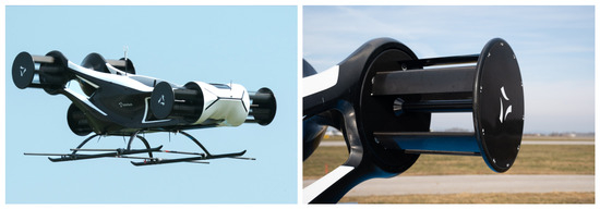
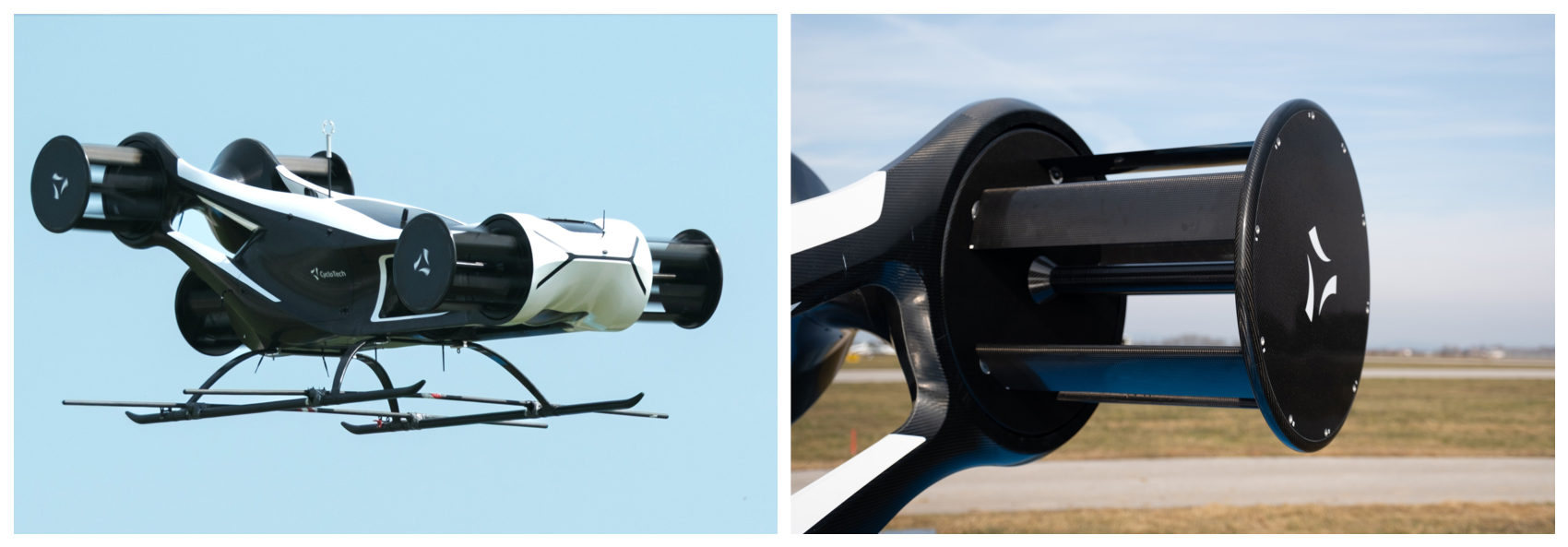
Recent advances in lightweight electric propulsion, batteries, composite materials, and computational fluid dynamics (CFD) have accelerated the development of practical cyclorotor systems [1,3]. Among these, CycloTech GmbH (Linz, Austria) has demonstrated the most mature full-scale implementation through the BlackBird demonstrator (Figure 1), validating the feasibility of cyclorotor-based VTOL aircraft [5,6].

Figure 1. CycloTech “BlackBird” demonstrator (left: in flight; right: detail of cyclorotor unit). Image courtesy of CycloTech GmbH.

The cyclorotor concept is not new. Early aircraft concepts and experimental prototypes were proposed during the first half of the twentieth century [1,7], while the closely related Voith–Schneider marine propeller has demonstrated the long-term practical viability of cyclic blade-pitch propulsion [8,9]. Similar operating principles have also been successfully applied to cycloturbines, which represent the actively pitched counterpart of conventional vertical-axis wind turbines [10].

Several studies have investigated the influence of geometric parameters on cyclorotor performance. Yun et al. [2,11] combined momentum and blade-element theory with flight experiments on a scaled cyclocopter, while Hwang et al. [12] coupled response-surface optimization with two-dimensional CFD to optimize a six-bladed rotor under aerodynamic and structural constraints. Benedict et al. [13] and Kellen [14] conducted extensive experimental investigations of MAV-scale cyclorotors, whereas Hu et al. [15] examined the influence of blade aspect ratio and taper ratio on hover performance. Leger et al. [16] developed an analytical model of a hovering cyclorotor and applied it to investigate the effect of key geometric parameters on rotor performance.

A blade-number sweep at constant solidity has been carried out experimentally by Benedict et al. [17], who tested two-, three- and four-bladed MAV-scale cyclorotors of matched total blade area and found that fewer blades produced higher thrust and power loading. Their study covers a single solidity ($\sigma \approx 0.14$) on a 76 mm radius rotor at chord Reynolds numbers of $1.5$–$3.1\times {10}^4$. The present work extends this comparison to a crossed design spanning $\sigma =0.24$–0.60 at Reynolds numbers an order of magnitude higher, and Section 4.1 compares the two datasets in detail.

The analogous question has been studied more systematically for actively pitched vertical-axis wind turbines (VAWTs), whose blades experience continuously varying angles of attack similar to those of cyclorotors. Rezaeiha et al. [18] demonstrated that rotor solidity is the dominant geometric parameter governing aerodynamic performance, whereas blade number has only a minor influence once each turbine operates close to its optimal tip/speed ratio, and Miller et al. [19] and Parra et al. [20] confirmed the dominant role of solidity over a wide range of operating conditions. Sagharichi et al. [10] further showed that cyclic blade pitching substantially mitigates the efficiency losses associated with high solidity—a mechanism directly relevant to cyclorotors, whose blades are cyclically pitched by design. These results provide a useful expectation against which the present cyclorotor matrix can be assessed.

The work most closely related to the present study is that of Xisto et al. [3,21], who performed a systematic two-dimensional URANS analysis of a large-scale cyclorotor validated against experimental measurements. Their study investigated the effects of airfoil thickness, blade number, chord-to-radius ratio, and pitching-axis location, showing that increasing blade number at constant blade chord reduced power loading and that a chord-to-radius ratio close to 0.5 produced the highest efficiency when compared at constant disk loading. However, because blade number was varied at constant chord, blade number and solidity changed together, and Xisto et al. [21] concluded that the effect of increasing blade number at constant rotor solidity was not evident from their results and that an independent study was required to resolve it. The present work carries out that study.

This is done through a two-dimensional URANS parametric investigation in which blade number (2–8) and rotor solidity (0.24–0.60) are varied independently across 26 geometrically feasible design points, at constant rotor radius and rotational speed. Because solidity also sets the thrust—and therefore the disk loading—at fixed rotational speed, performance is assessed both in terms of power loading and in terms of a disk-loading-normalized efficiency, so that changes in aerodynamic efficiency can be distinguished from changes in operating point. The results provide practical guidance for the preliminary aerodynamic design of cyclorotors.

2. Materials and Methods

2.1. Cyclorotor Geometry and Blade Kinematics

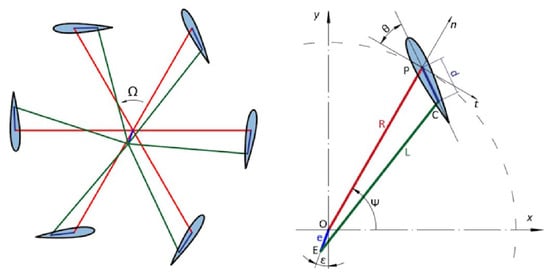
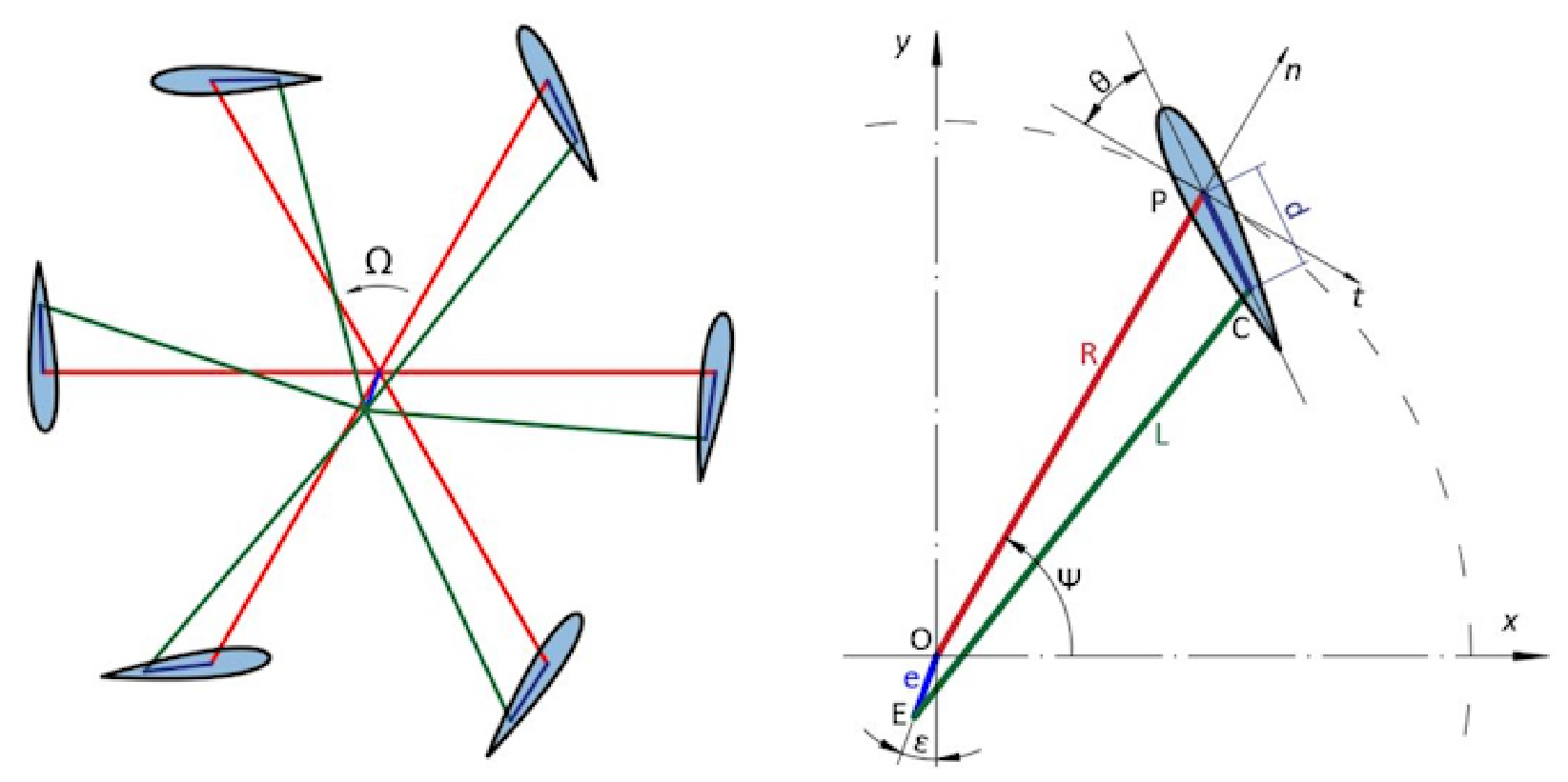
The study considers a two-dimensional cycloidal rotor based on the IAT21 rotor [5] operating in hover under quiescent atmospheric conditions. Table 1 lists the geometric and kinematic parameters of the rotor, and Figure 2 shows the baseline six-bladed configuration together with all geometric variables.

Table 1. Rotor parameters—IAT21 L3 validation case.

Parameter	Value
Airfoil	NACA 0016
Rotor diameter, D (m)	1.2
Rotor radius, R (m)	0.6
Span, b (m)	1.2
Chord, c (m)	0.3
Normalized pitching-axis position along the chord, $x_p$	0.35
Number of blades, N	6
Length of control rod, L (m)	0.61
Magnitude of eccentricity, e (m)	0.072
Phase angle of eccentricity, $\epsilon$ (°)	0
Crank arm length, d (m)	0.12

Figure 2. Geometry and eccentric-linkage pitching mechanism used to prescribe blade pitching motion. $R=\overline{OP}$ denotes rotor radius, $e=\overline{OE}$ eccentricity, $d=\overline{PC}$ crank-arm length, $L=\overline{EC}$ connecting-link length, $\mathrm{\Psi }$ blade azimuth angle, $\theta$ blade pitch angle, and $\Omega$ rotor rotational velocity.

The objective of the study is to isolate the independent effects of blade number and solidity on hover performance. Blade number was varied between $N=2$ and $N=8$, while rotor solidity,

$$\sigma ={\displaystyle \frac{Nc}{2\pi R}},$$

(1)

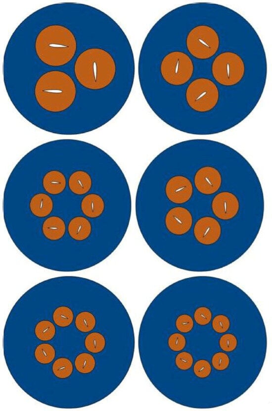
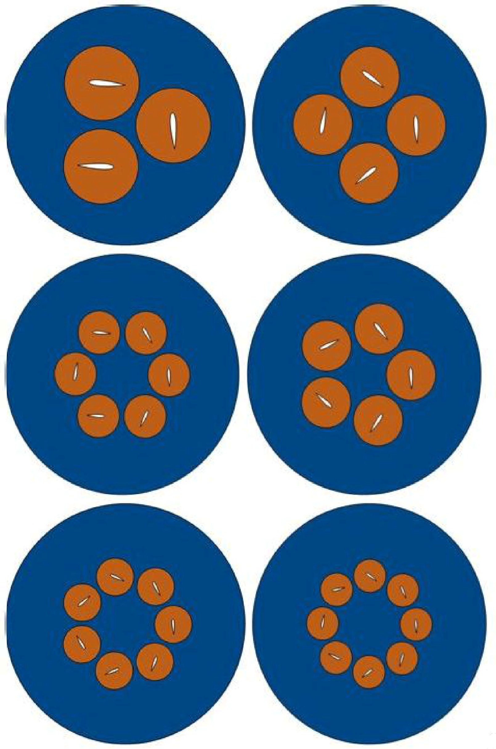
was prescribed independently over the range $0.24\le \sigma \le 0.60$, subject to the geometric feasibility constraints discussed in Section 2.2. For each $(N,\sigma )$ combination, the corresponding blade chord was obtained directly from the above expression while all remaining operating and geometric parameters were kept unchanged. Figure 3 illustrates the resulting constant-solidity family.

Figure 3. Rotor configurations at constant solidity ($\sigma =0.36$) for blade counts $N=3$ to 8. The blade chord decreases as the blade number increases while the rotor solidity remains constant.

Maintaining constant rotor radius, rotational speed and operating conditions across the entire design matrix ensures that the observed variations in aerodynamic performance originate solely from changes in blade number and solidity, thereby allowing their individual contributions to be distinguished.

Blade pitching motion is generated using an eccentric-linkage mechanism, which represents the kinematic solution adopted in modern CycloTech/IAT21 rotors [5]. The mechanism converts the constant rotational motion of the rotor hub into a periodic variation of blade pitch angle during each revolution. The kinematic formulation follows the model proposed by Leger et al. [16].

The instantaneous blade pitch angle is determined from the linkage geometry and blade azimuthal location $\mathrm{\Psi }$ according to

$$\theta ={\displaystyle \frac{\pi }{2}}-\arcsin \left[{\displaystyle \frac{e}{a}}\cos (\mathrm{\Psi }+\epsilon )\right]-\arccos \left[{\displaystyle \frac{a^2+d^2-L^2}{2ad}}\right],$$

(2)

where

$$a=\sqrt{e^2+R^2+2eR\sin (\mathrm{\Psi }+\epsilon )}.$$

(3)

The prescribed pitching motion was implemented in ANSYS Fluent 2024 R2 through a user-defined function (UDF), which updated the instantaneous pitch angle of each blade at every time step according to Equations (2) and (3). The linkage geometry of Table 1 gives a peak-to-peak pitch amplitude of approximately $75°$, identical for all configurations in the matrix.

2.2. Design Space and Parameter Matrix

Rotor solidity is defined in Equation (1), and the blade chord for a given $(N,\sigma )$ combination follows directly as

$$c={\displaystyle \frac{2\pi R\sigma }{N}}.$$

(4)

The parameter space comprises blade counts from $N=2$ to $N=8$ and solidities from $\sigma =0.24$ to $\sigma =0.60$. For each $(N,\sigma )$ combination, the blade chord is obtained from Equation (4); all remaining geometric and operating parameters are held constant.

At high solidity and low blade count, neighboring blade subdomains may overlap, preventing construction of a valid sliding-mesh topology. A geometric feasibility criterion is therefore introduced. For N equally spaced blades, the maximum subdomain radius is $R_{1,\max }=R\sin (\pi /N)$. Reducing this by the fractional inter-subdomain gap g and requiring the blade chord to fit within the remaining radius with a fractional wake margin m aft of the trailing edge gives the maximum admissible chord-to-radius ratio

$${\left({\displaystyle \frac{c}{R}}\right)}_{\max }={\displaystyle \frac{(1-m)(1-g)\sin (\pi /N)}{1-x_p}},$$

(5)

where $x_p$ is the normalized pitching-axis position along the chord. Applying this criterion to the full $7\times 5$ grid reduces the design space to the 26 geometrically feasible configurations shown in Table 2; infeasible configurations are highlighted in red.

Table 2. Feasible blade-number/solidity combinations. Green cells indicate the 26 geometrically feasible configurations used in the study; red cells indicate configurations excluded as geometrically infeasible by Equation (5).

	$\mathit{\sigma }=0.24$	$\mathit{\sigma }=0.36$	$\mathit{\sigma }=0.48$	$\mathit{\sigma }=0.60$	$\mathit{\sigma }=0.72$
$\mathit{N}$	$\mathit{c}/\mathit{R}$	$\mathit{c}/\mathit{R}$	$\mathit{c}/\mathit{R}$	$\mathit{c}/\mathit{R}$	$\mathit{c}/\mathit{R}$
2	0.75	1.13	1.51	1.88	2.26
3	0.50	0.75	1.01	1.26 *	1.51
4	0.38	0.57	0.75	0.94	1.13
5	0.30	0.45	0.60	0.75	0.90
6	0.25	0.38	0.50	0.63	0.75
7	0.22	0.32	0.43	0.54	0.65
8	0.19	0.28	0.38	0.47	0.57

* Borderline case; criterion applied with $g=0.04$ and $m=0.015$. This configuration ($N=3$, $\sigma =0.60$) also shows anomalous aerodynamic behavior and is discussed separately in Section 4.5.

2.3. Computational Domain and Mesh

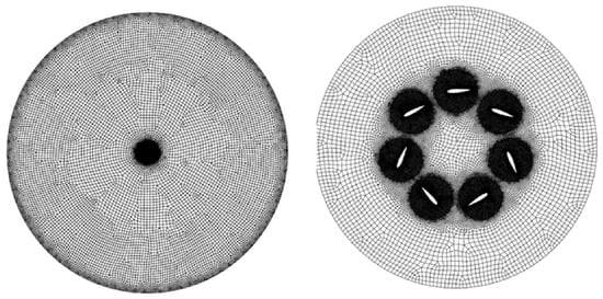
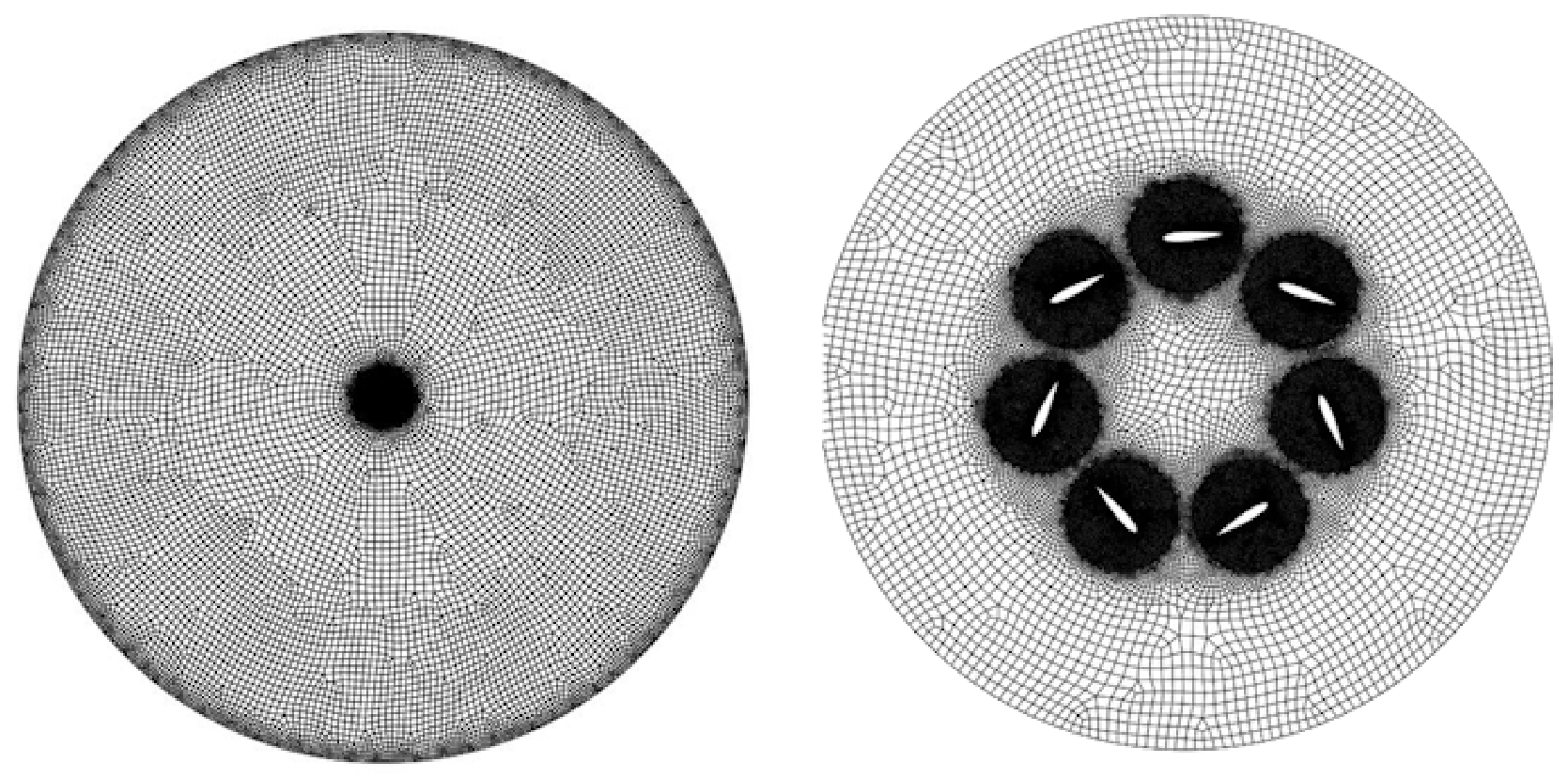
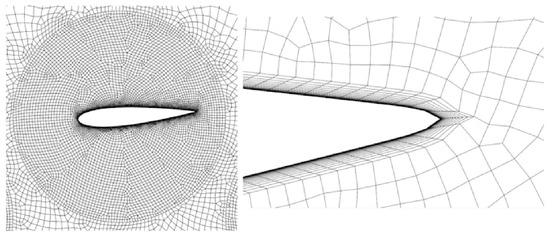
The two-dimensional domain consists of a stationary outer region and a rotating inner region coupled by a sliding (non-conformal) interface (Figure 4, left). The outer boundary is a circle of radius 20 m ($33.3R$) from the rotor center, treated as a pressure far-field boundary condition, which permits the recirculating inflow characteristic of a hovering cyclorotor. The inner rotating region has a radius of $1.5$ m ($2.5R$) and contains the individual blade subdomains shown in Figure 3; Figure 4 (right) shows the rotating-region mesh for the six-bladed configuration.

Figure 4. (Left): computational domain mesh (outer stationary far-field region, radius 20 m/$33.3R$). (Right): rotating-region mesh for the six-bladed configuration, showing the individual sliding-mesh subdomains around each blade.

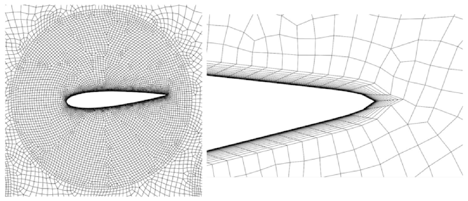
The blade surfaces carry an inflation layer with first-layer thickness $5\times {10}^{-6}$ m, 20 layers and a growth rate of 1.2, targeting $y^{+}\lesssim 1$ as required by the turbulence model (Section 2.4); Figure 5 shows the blade mesh (left) and a detail of this boundary-layer mesh near the blade trailing edge (right). Each blade surface was discretized with a chord-proportional node count rather than a fixed absolute element size, to maintain consistent chordwise resolution across all solidities.

Figure 5. (Left): blade surface mesh with inflation layer. (Right): detail of the boundary-layer (inflation) mesh at the blade trailing edge.

Because rotor radius and rotational speed are held fixed across the entire matrix, the blade-relative velocity scale $\Omega R=31.4$ m/s is identical for every configuration, so wall shear stress varies across the design space only through the Reynolds-number dependence of the skin-friction coefficient and through changes in blade chord. The achieved wall $y^{+}$ was extracted at the end of the final revolution for three configurations spanning the full chord range: area-averaged values of 0.27, 0.26 and 0.32 for $c=113$ mm ($N=8$, $\sigma =0.24$), $c=151$ mm ($N=6$, $\sigma =0.24$) and $c=754$ mm ($N=3$, $\sigma =0.60$), respectively, with facet maxima of 1.12, 1.11 and 0.98. The near-wall resolution is therefore essentially uniform across a 6.7-fold variation in Reynolds number and a 6.7-fold variation in chord, and satisfies the target $y^{+}\lesssim 1$ required by the turbulence model at both extremes of the design space. The 20-layer inflation stack has a total thickness of 0.93 mm, corresponding to $y^{+}\approx 96$, so the viscous sublayer and buffer layer are fully resolved and the stack extends into the logarithmic region. Combined with the chord-proportional surface discretization noted above, the near-wall and chordwise mesh resolution are non-dimensionally similar for every $(N,\sigma )$ configuration; this is the basis for applying the single grid-convergence study of Section 3.2 to the full matrix.

2.4. Numerical Methodology and Data Reduction

Simulations were performed in ANSYS Fluent using the pressure-based incompressible solver. Turbulence was modeled with the shear-stress transport (SST) k–$\omega$ model, applied in fully turbulent mode throughout the matrix. This is appropriate here for three reasons. The matrix spans chord Reynolds numbers from $2.4\times {10}^5$ to $1.6\times {10}^6$, so only the smallest-chord configurations approach the regime in which laminar separation bubbles govern NACA 0016 section behavior. The blade kinematics force early transition, since the blades operate under cyclic pitch amplitudes of approximately $\pm 37°$ with strong adverse pressure gradients and periodic leading-edge separation. Finally, the ambient turbulence level within the rotor region is elevated, as each blade repeatedly traverses the wakes of its predecessors; this differs substantially from the low-freestream-turbulence conditions for which correlation-based transition models are calibrated. The same closure was adopted by Xisto et al. [3] for this rig family. The residual sensitivity to this choice is quantified in Section 4.5.

Pressure–velocity coupling was achieved using the SIMPLE algorithm. Convection terms in momentum and turbulence equations were discretized using second-order upwind schemes, while temporal integration employed a second-order implicit formulation. The rotor was advanced with a constant angular increment of $0.5°$ per time step, corresponding to $\Delta t=1.667\times {10}^{-4}$ s at 500 RPM and yielding 720 time steps per revolution. Each simulation was performed for approximately six rotor revolutions (4320 time steps). Aerodynamic forces ($F_x$, $F_y$) and the moment about the rotor axis (Q) were recorded at every time step for both the complete rotor and each individual blade. Since the simulations were performed in two dimensions, Fluent reports forces and moments per unit span; these quantities were therefore treated as span-normalized throughout the parametric study and converted to dimensional values only for the validation comparison against experimental data.

The aerodynamic performance of each configuration was evaluated from cycle-averaged forces and torque. The averaging window was defined from complete rotor revolutions: the last three complete revolutions were used whenever available, falling back to the last two complete revolutions for runs that did not reach six full revolutions. The resultant thrust was computed from the cycle-averaged force components following the convention of Schwaiger and Wills [5],

$$T=\sqrt{{⟨F_x⟩}^2+{⟨F_y⟩}^2},$$

(6)

which avoids the artificial increase in apparent thrust from averaging the instantaneous force magnitude since lateral force oscillations cancel over a full rotor revolution. Aerodynamic power was obtained from the cycle-averaged rotor torque, $P=\Omega |⟨Q⟩|$, where the absolute value accounts for the reaction torque opposing rotor rotation. The non-dimensional performance metrics were defined as

$$C_T={\displaystyle \frac{T}{\rho A{(\Omega R)}^2}},C_P={\displaystyle \frac{P}{\rho A{(\Omega R)}^3}},PL={\displaystyle \frac{T}{P}},$$

(7)

where $A=2Rb$ is the projected rotor area.

For comparison at matched operating conditions (Section 3.6), two further non-dimensional quantities were evaluated at every design point. Because rotor radius, span and rotational speed are held constant across the matrix, disk loading follows directly from the thrust coefficient.

$$DL={\displaystyle \frac{T}{A}}=C_T\rho {(\Omega R)}^2,$$

(8)

and a two-dimensional figure of merit, referenced to the ideal (momentum-theory) induced power at that disk loading, was defined as

$$F{M}_{2\mathrm{D}}={\displaystyle \frac{C_T^{3/2}}{\sqrt{2}{C}_P}}.$$

(9)

$F{M}_{2\mathrm{D}}$ is reported as a relative ranking metric only: since it is evaluated from two-dimensional coefficients, it inherits the systematic bias quantified in Section 3.1 and can exceed unity for the lowest-blade-number configurations (Section 3.6).

Cycle-to-cycle periodicity was assessed independently of the solver residuals using the standard deviation of the revolution-averaged thrust coefficient within the averaging interval, normalized by its mean value. This metric is reported for every design point in Section 3.3.

3. Results

3.1. Validation Against the IAT21 L3 Rotor

The numerical model was validated against the IAT21 L3 cycloidal rotor reported by Schwaiger and Wills [5] and, with the same rig, by Xisto et al. [3,21]. The validation geometry comprises $N=6$ blades of chord $c=0.3$ m at rotor radius $R=0.6$ m (chord-to-radius ratio $c/R=0.5$, solidity $\sigma =0.48$), the same eccentric-linkage pitching mechanism as Section 2.1, and a pitching-axis location at 35% of chord [3]. Air density was set to $\rho =1.225$ kg/m³, matching the reference study. Seven rotor speeds (200, 300, 400, 500, 600, 750 and 1000 RPM) were simulated, spanning the range covered by the published simulation and experimental curves, and each case was processed through the identical pipeline described in Section 2.4. Because the solver integrates forces over an implicit unit span, the raw outputs were rescaled by the ratio of the rig’s true span to that unit span ($b/1\mathrm{m}=1.2$) before comparison with the dimensional literature values.

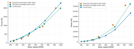
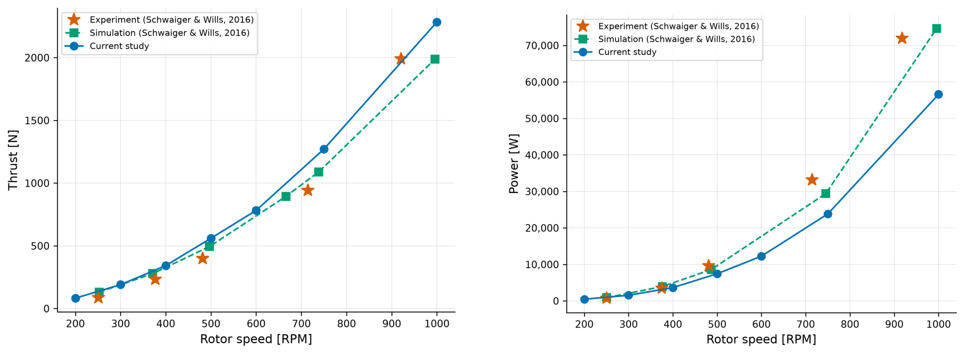
Figure 6 shows a comparison between the computed results and the experimental data for the IAT21 L3 rotor configuration [5].

Figure 6. Thrust (left) and power consumption (right) vs. rotor speed, IAT21 L3 validation rig: present CFD vs. the simulation and experimental curves of Schwaiger and Wills [5].

The present model overestimates thrust and underestimates power consumption, although the computed and experimental trends are consistent. Table 3 quantifies this comparison at each simulated rotor speed, interpolating the experimental curves of Schwaiger and Wills [5] onto the simulated RPM values.

Table 3. Quantitative validation against Schwaiger and Wills [5]: computed (CFD) and experimental (exp) thrust and power at each simulated rotor speed, with signed percentage deviation.

RPM	${\mathit{T}}_{\mathbf{CFD}}$ [N]	${\mathit{T}}_{\mathbf{exp}}$ [N]	$\mathbf{\Delta }\mathit{T}$ [%]	${\mathit{P}}_{\mathbf{CFD}}$ [W]	${\mathit{P}}_{\mathbf{exp}}$ [W]	$\mathbf{\Delta }\mathit{P}$ [%]
200	83.3	86.5	$-3.7$	464	754	$-38.4$
300	190.6	143.7	$+32.7$	1546	1837	$-15.8$
400	342.6	270.2	$+26.8$	3644	4934	$-26.1$
500	560.6	441.8	$+26.9$	7446	11,555	$-35.6$
600	782.7	674.9	$+16.0$	12,252	21,629	$-43.4$
750	1271.3	1122.3	$+13.3$	23,853	39,933	$-40.3$
1000	2284.4	1991.2	$+14.7$	56,585	71,946	$-21.3$

Over the 300–1000 RPM range, thrust is over-predicted by 21.7% on average (normalized RMSE 19.8%) and power under-predicted by 30.4% (normalized RMSE 39.6%), implying a power-loading bias of a factor 1.75. Both deviations are single-signed across this range. The 200 RPM case is excluded from these aggregates since the reference simulation and experiment themselves disagree by a comparable margin at that speed; it is also the only point at which the thrust deviation changes sign ($-3.7\%$).

The overestimation of thrust is attributed to the two-dimensional approximation of the rotor, in which three-dimensional losses—most notably the blade-tip vortex system and the associated induced losses—are neglected. The underestimation of power reflects the fact that only the aerodynamic power component is computed: the parasitic power required to rotate the rotor frame is not accounted for, and three-dimensional losses are again absent [3]. Consistent with this interpretation, the thrust deviation decreases with rotational speed, from approximately 33% at 300 RPM to 15% at 1000 RPM, as the induced flow develops and the relative significance of the missing three-dimensional mechanisms diminishes. A bias of the same sign and comparable magnitude has been reported independently for the identical L3 rig by Xisto et al. [3] and, for a different cyclorotor geometry and solver, by Hu et al. [15].

Section 4.5 shows that this bias is not uniform across the design matrix. All parametric conclusions in Section 3 and Section 4 are therefore stated in comparative terms—trends, rankings and the location of optima—rather than as absolute performance predictions.

3.2. Spatial and Temporal Convergence

A formal three-level grid convergence study was performed following Celik et al. [22] for the configuration $N=6$, $\sigma =0.48$, which coincides with the validation geometry of Section 3.1 and whose chord-to-radius ratio ($c/R=0.5$) lies near the middle of the tested range. Three systematically refined meshes of approximately $1.5\times {10}^5$, $2.6\times {10}^5$ and $4.2\times {10}^5$ cells were generated with identical boundary-layer parameters. The thrust coefficient converges monotonically with refinement, giving a Grid Convergence Index of 1.1% for the finest mesh.

As set out in Section 2.3, the meshing procedure is parametric rather than fixed in absolute terms: blade surfaces carry a chord-proportional node count, and the measured near-wall resolution is near-uniform across the matrix because $\Omega R$ is held constant. The grid-convergence index established here therefore transfers to the remaining configurations in non-dimensional terms. As a per-configuration indicator, the cycle-to-cycle periodicity metric of Section 2.4 is reported for every design point in Table 4. It remains below $3.2\%$ for 22 of the 26 configurations; the two largest values, $5.2\%$ at $N=3,\sigma =0.60$ and $6.0\%$ at $N=4,\sigma =0.60$, occur at the largest chord-to-radius ratios, where the flow is least periodic and where the model is in any case least reliable (Section 4.5). For the grid-convergence configuration itself ($N=6$, $\sigma =0.48$) the metric is $1.30\%$, at the lower end of the $1.30$–$2.56\%$ band spanned by the three meshes of the convergence study at the same simulation length; the per-configuration and grid-convergence assessments are therefore mutually consistent.

Table 4. Hover performance across the 26-point N–$\sigma$ matrix: chord-to-radius ratio, thrust and power coefficients, power loading, two-dimensional figure of merit $F{M}_{2\mathrm{D}}$ (Equations (8) and (9)), disk loading, blade Reynolds number and cycle-to-cycle periodicity.

N	$\mathit{\sigma }$	$\mathit{c}/\mathit{R}$	${\mathit{C}}_{\mathit{T}}$	${\mathit{C}}_{\mathit{P}}$	PL [N/W]	${\mathit{FM}}_{2\mathbf{D}}$	DL [N/m2]	$\mathit{Re}/{10}^5$	Per. [%]
2	0.24	0.75	0.273	0.101	0.0861	0.999	330	9.62	1.20
2	0.36	1.13	0.335	0.129	0.0827	1.064	405	14.43	0.64
3	0.24	0.50	0.253	0.092	0.0874	0.977	306	6.41	1.30
3	0.36	0.75	0.309	0.124	0.0792	0.978	373	9.62	1.30
3	0.48	1.01	0.331	0.168	0.0627	0.800	400	12.83	3.00
3	0.60	1.26	0.256	0.220	0.0370	0.416	309	16.03	5.21
4	0.24	0.38	0.238	0.087	0.0869	0.943	288	4.81	2.64
4	0.36	0.57	0.294	0.116	0.0805	0.970	356	7.21	2.60
4	0.48	0.75	0.335	0.155	0.0688	0.885	405	9.62	2.61
4	0.60	0.94	0.329	0.205	0.0510	0.651	398	12.02	6.00
5	0.24	0.30	0.229	0.085	0.0861	0.914	276	3.85	2.22
5	0.36	0.45	0.282	0.112	0.0801	0.945	341	5.77	1.88
5	0.48	0.60	0.333	0.151	0.0703	0.902	403	7.70	0.90
5	0.60	0.75	0.369	0.202	0.0581	0.784	446	9.62	2.12
6	0.24	0.25	0.219	0.079	0.0887	0.923	265	3.21	2.67
6	0.36	0.38	0.270	0.106	0.0815	0.941	327	4.81	3.17
6	0.48 †	0.50	0.305	0.130	0.0746	0.915	369	6.39	1.30
6	0.60	0.63	0.340	0.170	0.0636	0.823	411	8.02	1.85
7	0.24	0.22	0.214	0.077	0.0886	0.911	259	2.75	3.08
7	0.36	0.32	0.263	0.102	0.0821	0.935	318	4.12	3.85
7	0.48	0.43	0.292	0.121	0.0768	0.922	353	5.50	1.69
7	0.60	0.54	0.326	0.149	0.0695	0.881	394	6.87	1.49
8	0.24	0.19	0.209	0.076	0.0876	0.890	253	2.40	3.18
8	0.36	0.28	0.256	0.099	0.0827	0.930	310	3.61	3.85
8	0.48	0.38	0.282	0.115	0.0780	0.919	340	4.81	2.15
8	0.60	0.47	0.313	0.139	0.0715	0.888	378	6.01	1.99

^† Realized solidity $0.478$; see the footnote to Table 5.

Table 4. Hover performance across the 26-point N–$\sigma$ matrix: chord-to-radius ratio, thrust and power coefficients, power loading, two-dimensional figure of merit $F{M}_{2\mathrm{D}}$ (Equations (8) and (9)), disk loading, blade Reynolds number and cycle-to-cycle periodicity.

N	$\mathit{\sigma }$	$\mathit{c}/\mathit{R}$	${\mathit{C}}_{\mathit{T}}$	${\mathit{C}}_{\mathit{P}}$	PL [N/W]	${\mathit{FM}}_{2\mathbf{D}}$	DL [N/m2]	$\mathit{Re}/{10}^5$	Per. [%]
2	0.24	0.75	0.273	0.101	0.0861	0.999	330	9.62	1.20
2	0.36	1.13	0.335	0.129	0.0827	1.064	405	14.43	0.64
3	0.24	0.50	0.253	0.092	0.0874	0.977	306	6.41	1.30
3	0.36	0.75	0.309	0.124	0.0792	0.978	373	9.62	1.30
3	0.48	1.01	0.331	0.168	0.0627	0.800	400	12.83	3.00
3	0.60	1.26	0.256	0.220	0.0370	0.416	309	16.03	5.21
4	0.24	0.38	0.238	0.087	0.0869	0.943	288	4.81	2.64
4	0.36	0.57	0.294	0.116	0.0805	0.970	356	7.21	2.60
4	0.48	0.75	0.335	0.155	0.0688	0.885	405	9.62	2.61
4	0.60	0.94	0.329	0.205	0.0510	0.651	398	12.02	6.00
5	0.24	0.30	0.229	0.085	0.0861	0.914	276	3.85	2.22
5	0.36	0.45	0.282	0.112	0.0801	0.945	341	5.77	1.88
5	0.48	0.60	0.333	0.151	0.0703	0.902	403	7.70	0.90
5	0.60	0.75	0.369	0.202	0.0581	0.784	446	9.62	2.12
6	0.24	0.25	0.219	0.079	0.0887	0.923	265	3.21	2.67
6	0.36	0.38	0.270	0.106	0.0815	0.941	327	4.81	3.17
6	0.48 †	0.50	0.305	0.130	0.0746	0.915	369	6.39	1.30
6	0.60	0.63	0.340	0.170	0.0636	0.823	411	8.02	1.85
7	0.24	0.22	0.214	0.077	0.0886	0.911	259	2.75	3.08
7	0.36	0.32	0.263	0.102	0.0821	0.935	318	4.12	3.85
7	0.48	0.43	0.292	0.121	0.0768	0.922	353	5.50	1.69
7	0.60	0.54	0.326	0.149	0.0695	0.881	394	6.87	1.49
8	0.24	0.19	0.209	0.076	0.0876	0.890	253	2.40	3.18
8	0.36	0.28	0.256	0.099	0.0827	0.930	310	3.61	3.85
8	0.48	0.38	0.282	0.115	0.0780	0.919	340	4.81	2.15
8	0.60	0.47	0.313	0.139	0.0715	0.888	378	6.01	1.99

^† Realized solidity $0.478$; see the footnote to Table 5.

Table 5. Iso-Reynolds subsets: configurations with identical chord (and therefore identical $Re$, $AR$, k) but different N and $\sigma$.

Group	N	$\mathit{\sigma }$	c [m]	$\mathit{Re}$	${\mathit{C}}_{\mathit{T}}$	${\mathit{C}}_{\mathit{P}}$	$\mathit{PL}$ [N/W]
I ($AR=2.65$, $k=0.377$)	2	0.24	0.452	$9.62\times {10}^5$	0.273	0.101	0.0861
	3	0.36	0.452	$9.62\times {10}^5$	0.309	0.124	0.0792
	4	0.48	0.452	$9.62\times {10}^5$	0.335	0.155	0.0688
	5	0.60	0.452	$9.62\times {10}^5$	0.369	0.202	0.0581
II ($AR=5.31$, $k=0.188$)	4	0.24	0.226	$4.81\times {10}^5$	0.238	0.087	0.0869
	6	0.36	0.226	$4.81\times {10}^5$	0.270	0.106	0.0815
	8	0.48	0.226	$4.81\times {10}^5$	0.282	0.115	0.0780
III * ($AR\approx 4.0$, $k\approx 0.25$)	3	0.24	0.302	$6.41\times {10}^5$	0.253	0.092	0.0874
	6	0.478	0.300	$6.39\times {10}^5$	0.305	0.130	0.0746

* Group III chords differ by 0.4% because the realized solidity at $N=6$ is $\sigma =0.478$ rather than the nominal $0.48$ (Table 4); $Re$ and $AR$ are correspondingly matched to within the same 0.4%, not exactly.

Table 5. Iso-Reynolds subsets: configurations with identical chord (and therefore identical $Re$, $AR$, k) but different N and $\sigma$.

Group	N	$\mathit{\sigma }$	c [m]	$\mathit{Re}$	${\mathit{C}}_{\mathit{T}}$	${\mathit{C}}_{\mathit{P}}$	$\mathit{PL}$ [N/W]
I ($AR=2.65$, $k=0.377$)	2	0.24	0.452	$9.62\times {10}^5$	0.273	0.101	0.0861
	3	0.36	0.452	$9.62\times {10}^5$	0.309	0.124	0.0792
	4	0.48	0.452	$9.62\times {10}^5$	0.335	0.155	0.0688
	5	0.60	0.452	$9.62\times {10}^5$	0.369	0.202	0.0581
II ($AR=5.31$, $k=0.188$)	4	0.24	0.226	$4.81\times {10}^5$	0.238	0.087	0.0869
	6	0.36	0.226	$4.81\times {10}^5$	0.270	0.106	0.0815
	8	0.48	0.226	$4.81\times {10}^5$	0.282	0.115	0.0780
III * ($AR\approx 4.0$, $k\approx 0.25$)	3	0.24	0.302	$6.41\times {10}^5$	0.253	0.092	0.0874
	6	0.478	0.300	$6.39\times {10}^5$	0.305	0.130	0.0746

* Group III chords differ by 0.4% because the realized solidity at $N=6$ is $\sigma =0.478$ rather than the nominal $0.48$ (Table 4); $Re$ and $AR$ are correspondingly matched to within the same 0.4%, not exactly.

Each of the three meshes was also run for 12 revolutions. This reduced the cycle-to-cycle variation of the averaged thrust coefficient from 1.30–2.56% to 0.59–1.01%, while the mean performance coefficients changed only marginally. Six revolutions were therefore adopted for the parametric study, with the periodicity metric reported alongside each result so that the least periodic configurations can be weighted accordingly.

The rotor is advanced at $0.5°$ per time step, giving 720 steps per revolution and, since the pitch schedule is prescribed once per revolution, 720 steps per pitch cycle. This is the resolution established in the cyclorotor URANS literature, including Xisto et al. [3] on the same rig family, and corresponds to between 22 and 144 time steps per chord-convection time across the matrix.

3.3. Test Case Matrix

Table 4 lists all 26 feasible $(N,\sigma )$ design points together with the resulting chord-to-radius ratio, thrust and power coefficients, power loading, two-dimensional figure of merit, disk loading, blade Reynolds number ($Re=\rho \Omega Rc/\mu$, $\mu =1.81\times {10}^{-5}$ Pa s) and cycle-to-cycle periodicity. Because rotor radius and rotational speed are held fixed, $Re$ varies with chord as a direct consequence of each $(N,\sigma )$ combination, spanning $2.4\times {10}^5$ to $1.6\times {10}^6$, a factor of 6.7.

Two further quantities follow directly from the chord-to-radius ratio and are therefore not tabulated separately: since rotor radius and span are fixed, the blade aspect ratio is $AR=2/(c/R)$ and the blade reduced frequency is $k=(c/R)/2$. Over the tested range $c/R=0.19$–$1.26$, this gives $AR=1.6$–$10.6$ and $k=0.09$–$0.63$. A single geometric parameter thus governs virtual camber, blade unsteadiness and the magnitude of the three-dimensional correction simultaneously, a point returned to in Section 4.3 and Section 4.5.

3.4. Performance Maps

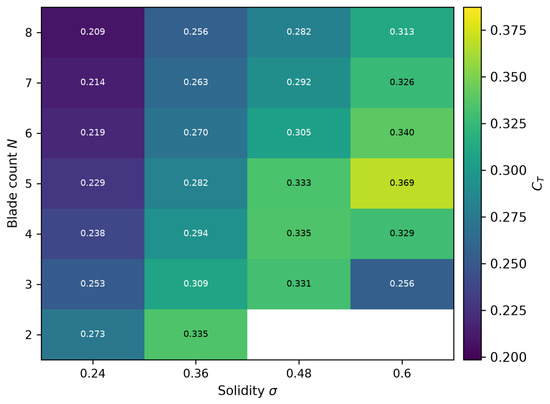
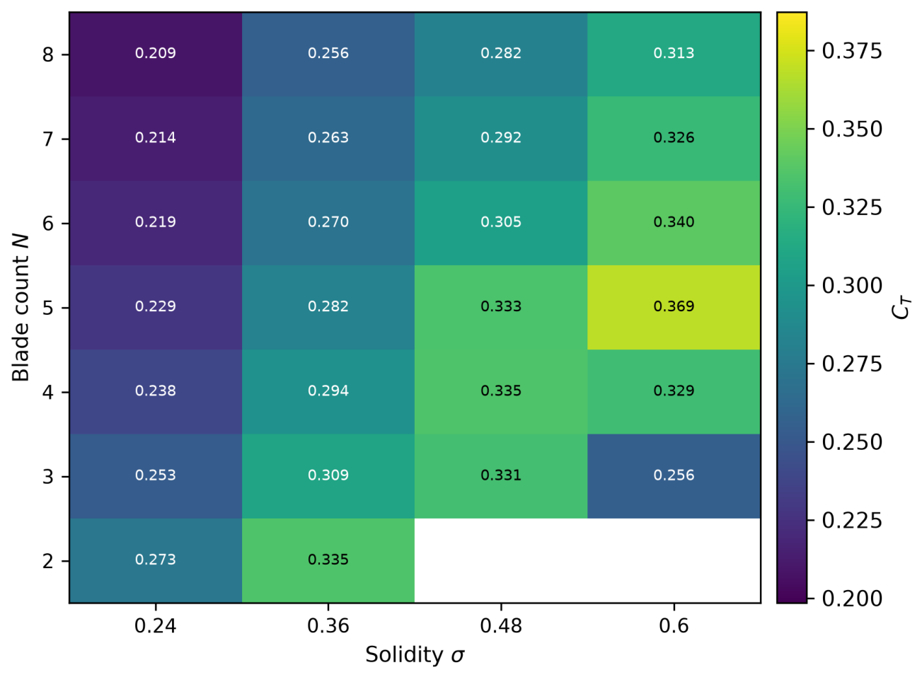
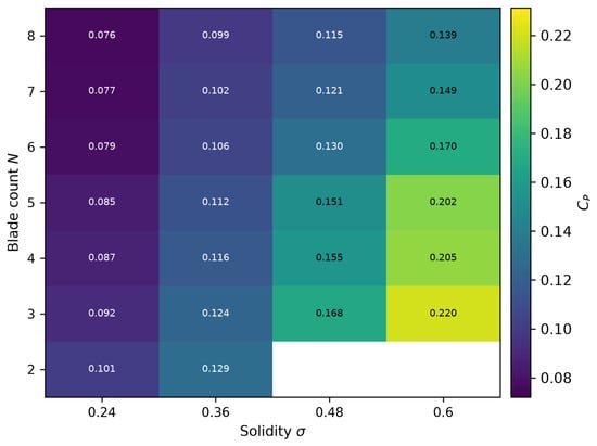
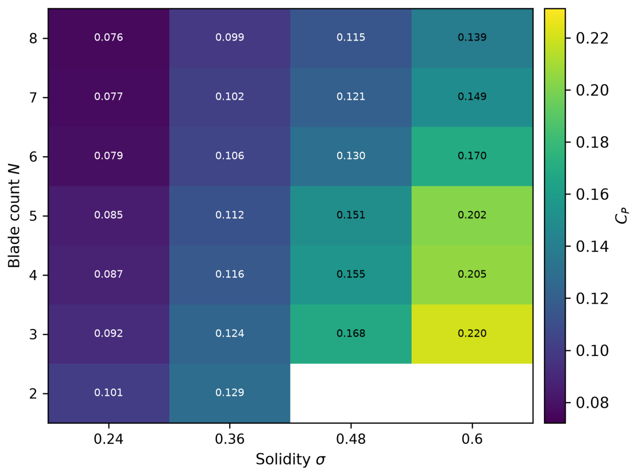
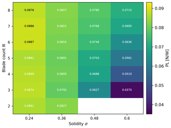
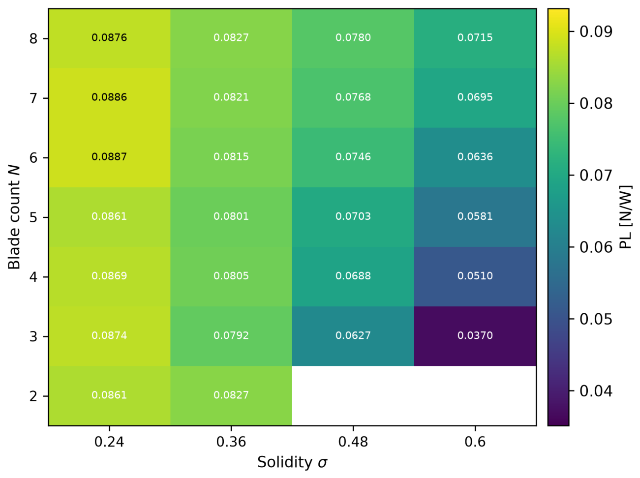
Figure 7, Figure 8 and Figure 9 map $C_T$, $C_P$ and power loading across the 26 design points. Both $C_T$ and $C_P$ rise with solidity, but $C_P$ rises more steeply, so the power-loading advantage of low solidity follows directly from power growing faster than thrust as $\sigma$ increases. Power loading ranges from 0.0370 to 0.0887 N/W; at the lowest tested solidity ($\sigma =0.24$), every blade count from $N=2$ to 8 reaches between 0.086 and 0.089 N/W, with no strong dependence on N. The global maximum (0.0887 N/W) occurs at $N=6$, marginally ahead of $N=7$ (0.0886 N/W)—a difference well within the cycle-to-cycle scatter of Table 4, so the two are jointly optimal. The lowest value (0.0370 N/W) occurs at $N=3$, $\sigma =0.60$, the borderline-feasible configuration discussed in Section 4.5.

Figure 7. Thrust coefficient $C_T$ in the N–$\sigma$ design space.

Figure 8. Power coefficient $C_P$ in the N–$\sigma$ design space.

Figure 9. Power loading in the N–$\sigma$ design space.

Section 3.6 shows that a substantial part of this power-loading trend reflects the change in disk loading with solidity rather than a change in aerodynamic efficiency.

3.5. Separated Effects of Blade Number and Solidity

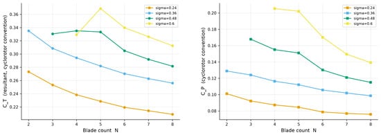
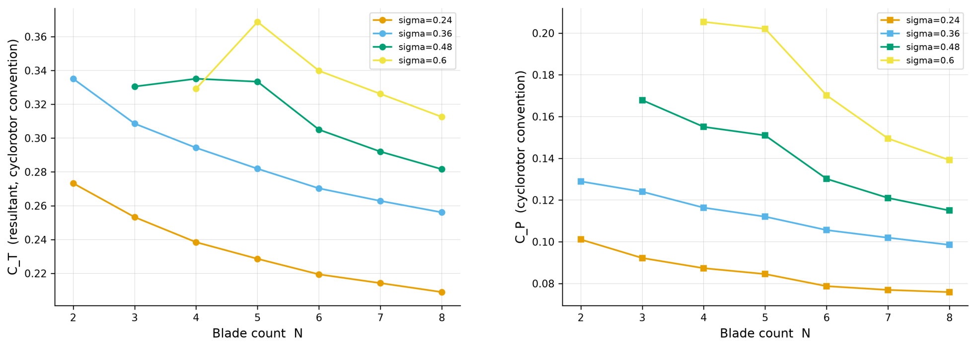
Figure 10 shows $C_T$ and $C_P$ against blade number at each tested solidity. At constant solidity both coefficients vary only weakly with blade number compared with their variation across solidity: at $\sigma =0.24$, $C_T$ spans 0.209–0.273 and $C_P$ spans 0.076–0.101 over the full $N=2$–8 range, a much narrower band than the corresponding spread across $\sigma$ at fixed N. Because each $\sigma$-sweep holds total blade area fixed while redistributing it across more, proportionally thinner blades, this isolates the effect of blade number from that of total blade area—a comparison not available in prior cyclorotor studies, which varied N at constant chord. Section 4.2 and Section 4.3 interpret this insensitivity.

Figure 10. Thrust coefficient (left) and power coefficient (right) vs. blade number N at constant solidity.

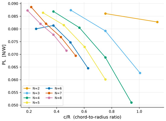
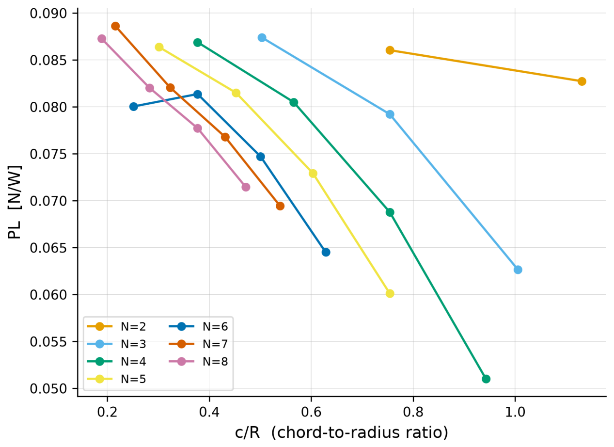
Figure 11 shows power loading against chord-to-radius ratio for each blade count. At every N, power loading decreases monotonically as $c/R$ increases across the tested range, with no interior optimum. This appears to contrast with the hump-shaped curve peaking near $c/R=0.5$ reported by Xisto et al. [3], but the disagreement is one of normalization rather than of physics: Xisto et al. compare at constant disk loading, whereas the present matrix fixes rotational speed. Normalized for disk loading (Section 3.6), an interior optimum consistent with theirs is recovered.

Figure 11. Power loading vs. chord-to-radius ratio at constant blade number.

3.6. Comparison at Matched Disk Loading

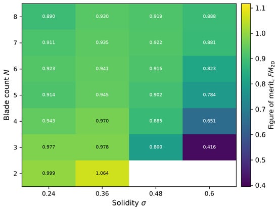
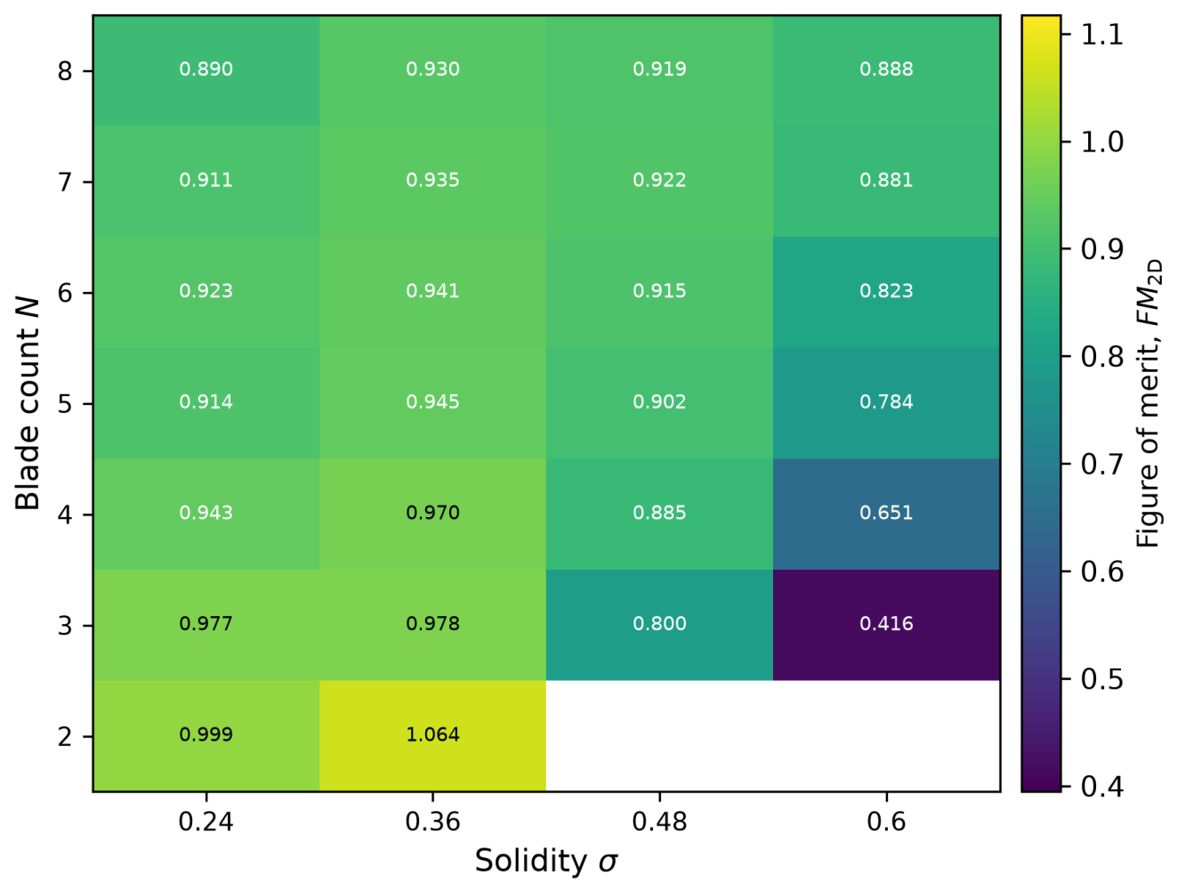
Power loading is not an efficiency metric in isolation: for an ideal rotor, momentum theory gives $P{L}_{\mathrm{ideal}}\propto D{L}^{-1/2}$, so comparing power loading between configurations at different disk loadings conflates aerodynamic efficiency with operating point. Because the present matrix runs at fixed rotational speed, solidity directly sets thrust and therefore disk loading (Equation (8)), so part of the trend in Section 3.4 is expected on these grounds alone. Figure 12 maps $F{M}_{2\mathrm{D}}$ across the design space.

Figure 12. Two-dimensional figure of merit $F{M}_{2\mathrm{D}}$ (Equation (9)) in the N–$\sigma$ design space.

Three findings follow. First, the solidity trend is substantially reduced once disk loading is accounted for: at $N=8$, power loading falls $18\%$ between $\sigma =0.24$ and $\sigma =0.60$ while $F{M}_{2\mathrm{D}}$ changes from $0.890$ to $0.888$, and at $N=7$ power loading falls $22\%$ while $F{M}_{2\mathrm{D}}$ remains within $0.88$–$0.94$. Configurations that happen to operate at nearly the same disk loading confirm this directly—$N=5,\sigma =0.36$ and $N=8,\sigma =0.48$ both operate near 340 N/m² and differ in power loading by $2.7\%$, against the 30–$40\%$ variation implied by the raw power-loading map of Figure 9.

Second, an interior optimum in $F{M}_{2\mathrm{D}}$ appears near $\sigma \approx 0.36$, consistently for every blade count from $N=4$ to $N=8$. This is invisible in the power-loading representation. Its amplitude (3–8 percentage points) is modest relative to the point-to-point scatter, but the increase from $\sigma =0.24$ to $\sigma =0.36$ is positive for all five independent blade counts ($N=4$–8), which under a sign test gives $p=0.031$, and it reconciles the present results with the chord-to-radius optimum reported by Xisto et al. [3].

Third, a genuine efficiency penalty remains after disk-loading normalization, but it is not described by chord-to-radius ratio alone. $F{M}_{2\mathrm{D}}$ lies within $0.88$–$1.06$ for 21 of the 26 configurations; the remaining five fall to $0.42$–$0.83$: $N=6,\sigma =0.60$ ($c/R=0.63$, $F{M}_{2\mathrm{D}}=0.823$), $N=3,\sigma =0.48$ ($1.01$, $0.800$), $N=5,\sigma =0.60$ ($0.75$, $0.784$), $N=4,\sigma =0.60$ ($0.94$, $0.651$) and $N=3,\sigma =0.60$ ($1.26$, $0.416$). All five combine high solidity ($\sigma \ge 0.48$) with a long blade chord, but neither variable accounts for the penalty on its own. At the fixed chord-to-radius ratio $c/R=0.754$—where Reynolds number, blade aspect ratio and reduced frequency are identical by construction (Group I of Table 5)—$F{M}_{2\mathrm{D}}$ still falls from $0.999$ to $0.784$ as solidity increases from $0.24$ to $0.60$, so the penalty is not removed by holding chord length fixed. Conversely, $N=2,\sigma =0.36$ has the second-longest chord in the matrix ($c/R=1.13$) yet the highest $F{M}_{2\mathrm{D}}$ of all. Regressed across the full matrix, chord-to-radius ratio alone accounts for $24\%$ of the variance in $F{M}_{2\mathrm{D}}$ and solidity alone for $36\%$, while their product accounts for $56\%$: the penalty is a joint effect of solidity and chord length, not a threshold in either.

The direction of the two-dimensional bias indicates that this penalty is understated rather than manufactured. Since $AR=2/(c/R)$, the longest-chord configurations also have the lowest aspect ratios, where the neglected three-dimensional losses—and hence the over-prediction of $F{M}_{2\mathrm{D}}$—are largest (Section 4.5). Within $\sigma =0.60$ the figure of merit nevertheless increases monotonically with blade number, from $0.416$ at $N=3$ to $0.888$ at $N=8$, that is, in the direction opposite to the bias. The efficiency penalty of the low-blade-number, long-chord corner is therefore a lower bound. This is the physically meaningful design boundary, discussed further in Section 4.3.

The two $N=2$ configurations warrant comment: $F{M}_{2\mathrm{D}}=0.999$ at $\sigma =0.24$ and $1.064$ at $\sigma =0.36$, the latter exceeding the momentum-theory ideal. This follows directly from the two-dimensional bias of Section 3.1—with thrust over-predicted and power under-predicted, $F{M}_{2\mathrm{D}}$ is over-predicted by a factor of approximately $1.9$—and from the low blade aspect ratio of these configurations ($AR=2.65$ and $1.77$), where the neglected three-dimensional effects are largest. $F{M}_{2\mathrm{D}}$ is therefore used strictly as a relative ranking metric within the two-dimensional dataset.

3.7. Isolation of Reynolds-Number Effects

Because $c=2\pi R\sigma /N$ (Equation (4)), all configurations sharing the same ratio $\sigma /N$ have identical chord and therefore identical Reynolds number, aspect ratio and reduced frequency; only the number of blades differs. The crossed design contains three such groups by construction, spanning nine of the twenty-six design points (Table 5).

Within Group I, Reynolds number and blade geometry are held exactly constant while solidity increases by a factor of 2.5 through blade number alone, and power loading falls by $32\%$ ($0.0861\to 0.0581$ N/W). Within Group II, solidity doubles at exactly constant Reynolds number and power loading falls $10\%$; within Group III it approximately doubles and power loading falls $15\%$. The solidity trend of Section 3.4 is therefore reproduced with Reynolds number held fixed, and cannot be a Reynolds-number artifact.

A second argument concerns the direction of the effect. In this design solidity and Reynolds number are positively correlated, since higher solidity implies a longer chord at fixed N, and higher Reynolds number reduces turbulent skin friction—roughly $32\%$ across the range spanned by the matrix. A Reynolds-number effect acting alone would therefore make high-solidity configurations appear more efficient, not less. Since they are nonetheless the least efficient (Section 3.6), the solidity penalty reported here is a lower bound: Reynolds-number variation can mask part of the trend, but cannot manufacture it.

It should be noted that, because $\log Re=\mathrm{const}+\log \sigma -\log N$, the Reynolds number is an exact deterministic function of the two design variables and is not statistically separable from them by regression. The iso-Reynolds subsets and the direction-of-effect argument are the available alternative.

3.8. Azimuthal Load Distribution

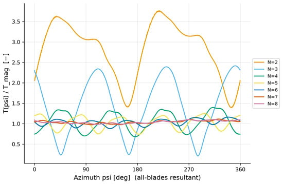
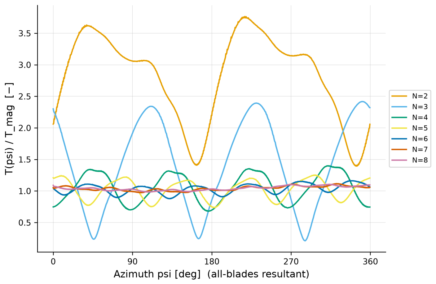
Per-blade force histories ($F_y$, $F_x$) were extracted at the azimuthal resolution of the simulation ($0.5°$/step) over the last complete revolution of each run, with blade azimuths referenced to a common origin at equal angular spacing $(i-1)\times 360°/N$ for blade i. Figure 13 overlays the instantaneous all-blades resultant magnitude $T\left(\psi \right)$ for $N=2$–8 at $\sigma =0.36$, normalized by the cycle-averaged T.

Figure 13. Instantaneous resultant thrust magnitude vs. azimuth, normalized by the cycle-averaged T, for $N=2$–8 at $\sigma =0.36$.

The number of ripple cycles per revolution equals the blade count. For $N\ge 4$ the peak-to-mean ratio falls below approximately 1.3 and continues to decrease with increasing N. For $N=2$ and $N=3$, however, the peak instantaneous thrust reaches approximately 3–4 times the cycle-averaged value, with troughs approaching zero for $N=3$.

Since rotor structure must be sized to the peak rather than the cycle-averaged aerodynamic load, the $N=2$ and $N=3$ configurations impose a design constraint that is not visible in the mean performance metrics of Section 3.4, Section 3.5 and Section 3.6; the fundamental excitation frequency equals the blade-passage frequency, $16.7$ Hz for $N=2$ and $25.0$ Hz for $N=3$ at 500 RPM. No structural or fatigue analysis has been performed, and quantifying the resulting penalty lies outside the scope of the present aerodynamic study.

3.9. Flow-Field Visualization

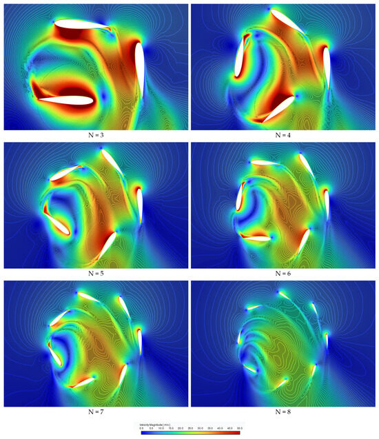
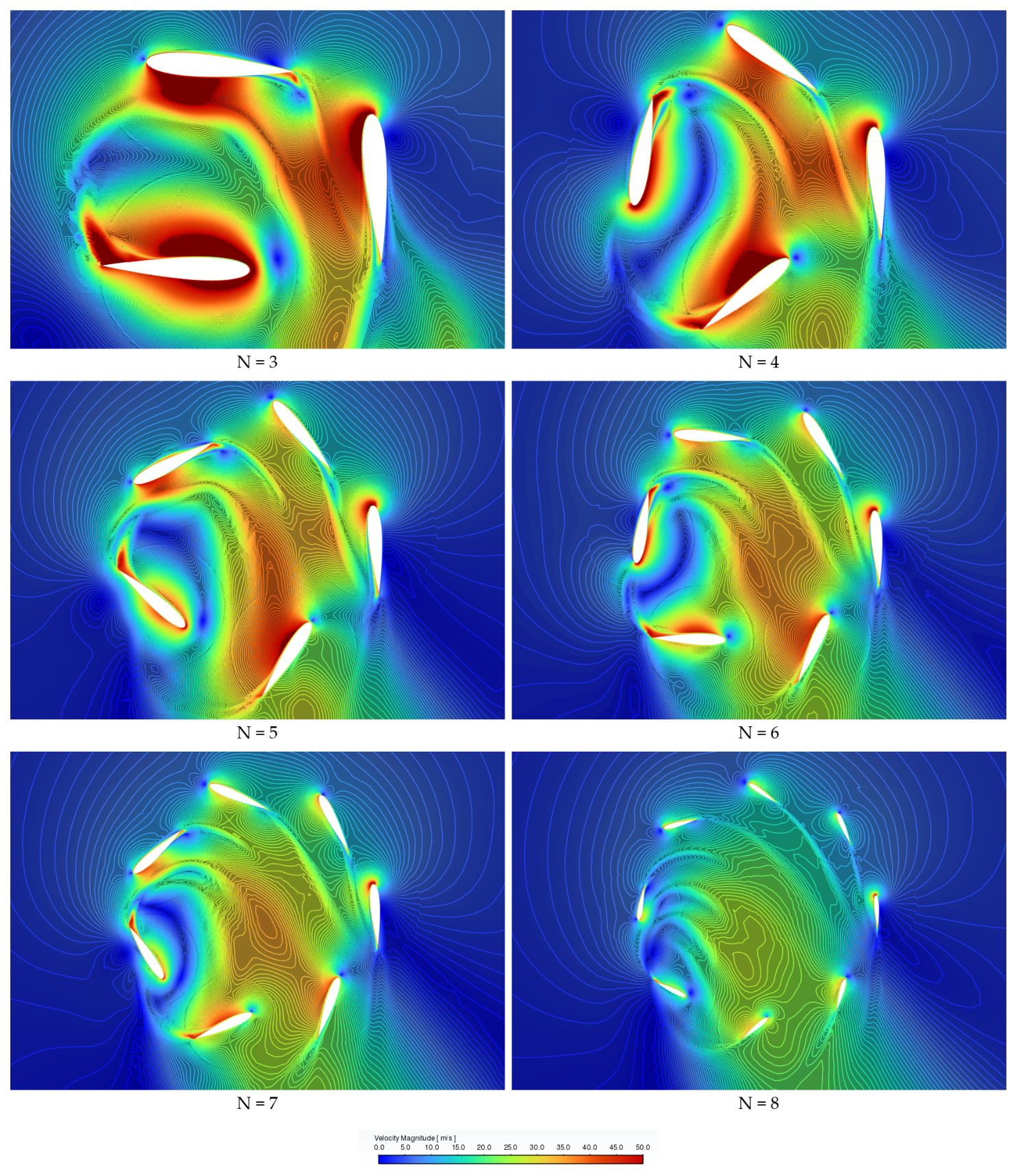
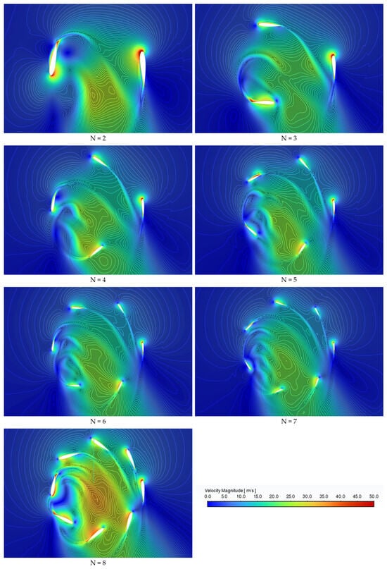
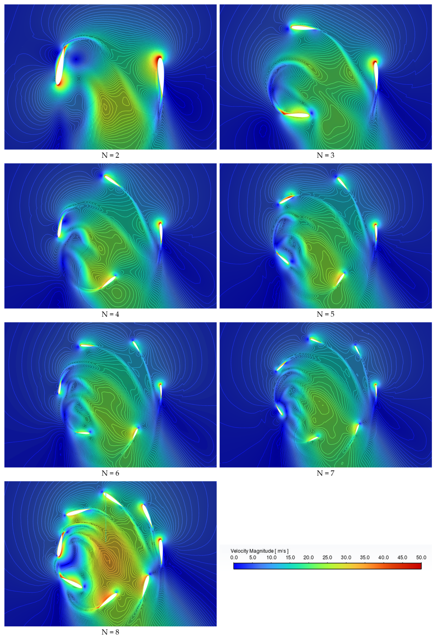
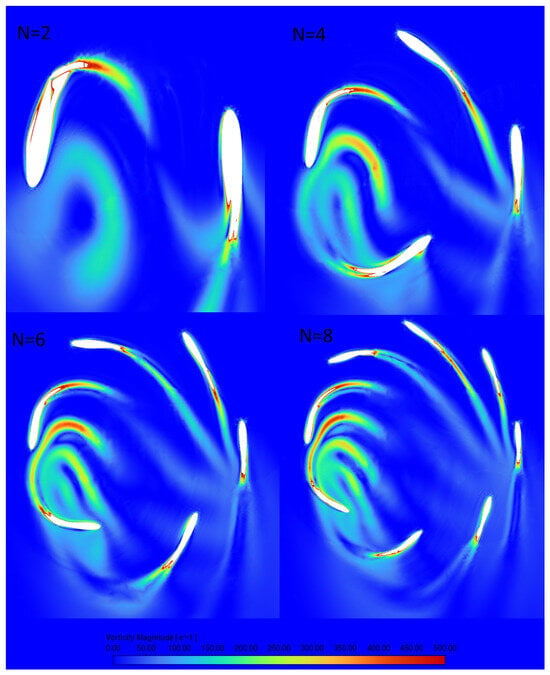
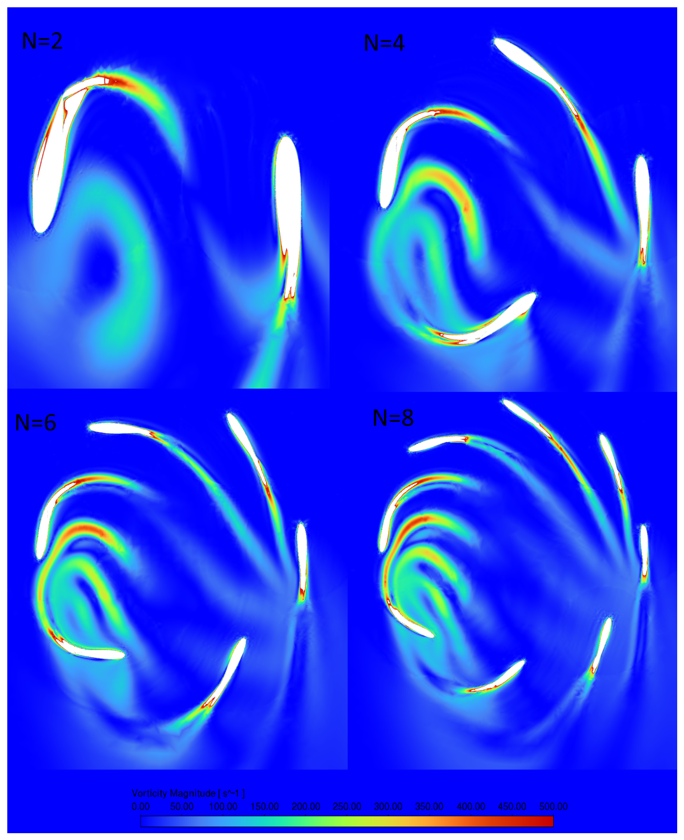
Figure 14 and Figure 15 show cycle-averaged velocity magnitude fields with iso-contours overlaid, rotor-region detail (color scale clipped at 50 m/s), for two representative solidities across the tested blade-count range. Figure 16 shows instantaneous vorticity magnitude in the rotor region for four representative blade counts at $\sigma =0.36$, at a common rotor phase and on a common color scale; this is discussed further in Section 4.3.

Figure 14. Cycle-averaged velocity magnitude with iso-contours, rotor-region detail, $\sigma =0.60$, $N=3$–8. Color scale clipped at 50 m/s.

Figure 15. Cycle-averaged velocity magnitude with iso-contours, rotor-region detail, $\sigma =0.24$, $N=2$–8. Color scale clipped at 50 m/s.

Figure 16. Instantaneous vorticity magnitude in the rotor region at $\sigma =0.36$ for $N=2$, 4, 6 and 8, at a common rotor phase and on a common color scale. As blade number increases, the individual blade wakes merge into a continuous vortical structure and each blade increasingly operates within the wake of its predecessor.

At the higher solidity ($\sigma =0.60$), the recirculating region behind each blade grows visibly larger and more irregular as blade number increases from $N=3$ to $N=8$, foreshadowing the blade–wake interference quantified from the vorticity field in Section 4.3.

At the lower solidity ($\sigma =0.24$), the wakes remain comparatively compact and well separated across the same blade-count range, consistent with the reduced blade-wake interference expected at the correspondingly wider blade spacing.

4. Discussion

4.1. Comparison with the Cyclorotor Literature

Xisto et al. [3], using the same rig family and the same 2D URANS sliding-mesh methodology, reported that increasing blade number reduces power loading. The two results are consistent: Xisto et al. varied N at constant chord, so their sweep simultaneously increased solidity and moved the operating point toward higher disk loading. Section 3.6 shows that once this operating-point effect is removed, the residual efficiency change with solidity is small except in the corner of the design space that combines high solidity with a long blade chord. Their earlier work [21] concluded that the effect of blade number at constant solidity was not evident and required an independent study; the present matrix supplies it, and the answer is that the effect is small (Section 3.5), for the reasons set out in Section 4.2.

Benedict et al. [17] varied blade number ($N=2$–4) at a single solidity ($\sigma \approx 0.14$) on a 76 mm radius MAV-scale rotor and reported that the two-bladed configuration achieved both the highest thrust and the highest power loading. The thrust trend agrees with the present results: at constant solidity, $C_T$ falls monotonically with blade number here as well (Table 4). The power-loading trend does not, and Reynolds number offers a plausible explanation. Because their sweep holds solidity rather than chord fixed, halving the chord from $N=2$ to $N=4$ also roughly halves the Reynolds number, from approximately $3.1\times {10}^4$ to $1.5\times {10}^4$—a regime in which MAV-scale profile drag is strongly Reynolds-sensitive. The present matrix spans a comparable Reynolds ratio at values roughly one to two orders of magnitude higher, where section drag is far less sensitive. The blade-number effect that Benedict et al. observe may therefore be amplified, at their scale, by a mechanism largely absent at the present scale.

4.2. Relation to Classical Rotor Theory

Classical hover theory decomposes rotor power into an induced contribution and a profile contribution [23,24]:

$$C_P=\kappa {\displaystyle \frac{C_T^{3/2}}{\sqrt{2}}}+{\displaystyle \frac{\sigma C_{d0}}{8}},$$

(10)

where $\kappa \ge 1$ is an induced-power correction factor for a physical rotor—the value fitted below falls under unity for the reason set out there and $C_{d0}$ an effective section drag coefficient. Because the induced term is super-linear in thrust while the profile term is linear in solidity and independent of thrust, this decomposition predicts that adding blade area at fixed rotational speed increases power faster than thrust, so that power loading and figure of merit must fall as solidity rises at fixed N—the trend underlying Section 3.4.

Fitting Equation (10) by least squares to the 22 configurations with $c/R\le 0.80$, excluding the four largest-chord geometries where virtual-camber and unsteady effects dominate, gives $\kappa =0.90$ and $C_{d0}=0.46$, with a coefficient of determination $R^2=0.952$ and an RMS residual of $6.0\%$ of the mean $C_P$. The fitted $\kappa$ falls below the $1.1$–$1.3$ typical of helicopter rotors, as expected from the way it was obtained: the fit is performed on two-dimensional coefficients, in which thrust is over-predicted and power under-predicted (Section 3.1). Correcting the induced term for both biases—the same compound factor of $1.93$ applied to $F{M}_{2\mathrm{D}}$ in Section 3.6—gives $\kappa =0.90\times 1.{217}^{3/2}/0.696=1.73$ and $C_{d0}=0.46/0.696=0.66$. The corrected $\kappa$ exceeds the classical helicopter range, which is consistent with a rotor whose induced velocity field is strongly non-uniform in azimuth and whose blades operate under $\pm 37°$ cyclic pitch with periodic leading-edge separation; the induced-power penalty of a cyclorotor should be expected to exceed that of a conventional rotor rather than to match it. Both corrected values are indicative rather than calibrated, since the bias factors are measured at a single configuration. From this fit, the profile-power fraction spans 13–$24\%$ of total power across the fitted configurations, increasing with solidity at fixed blade number: 18–$24\%$ at $N=8$, against 13–$16\%$ at $N=2$–3. The fraction is unaffected by the bias correction above, since the profile term and the total power scale identically under it.

The correspondence extends, in a useful way, to blade number. Blade number does not appear explicitly in Equation (10): at fixed solidity it enters classical rotor theory only through the tip-loss factor and finite-blade-number wake corrections, both of which are absent by construction in a two-dimensional formulation. Adding an explicit linear blade-number term to the fit raises $R^2$ only from $0.952$ to $0.959$, with a coefficient corresponding to a change in $C_P$ of $-0.008$ over the full $N=2\to 8$ range at fixed solidity—comparable to the residual scatter. Classical theory therefore predicts exactly the near-insensitivity of the mean coefficients to blade number reported in Section 3.5, and identifies the missing mechanisms as three-dimensional ones. As a further indicator, the blade-loading coefficient $C_T/\sigma$ falls monotonically with solidity at every blade number, from $1.14$ ($N=2$, $\sigma =0.24$) to $0.43$ ($N=3$, $\sigma =0.60$), indicating progressively lower mean sectional lift coefficient—and hence poorer effective lift-to-drag ratio—as solidity increases, the classical mechanism by which over-solid rotors lose figure of merit.

The correspondence is one of scaling rather than quantitative equivalence: the actuator area here is a rectangular projection, the blades operate under 1/rev cyclic pitch of order $\pm 37°$, and virtual-camber and reduced-frequency effects have no counterpart in classical hover theory. Equation (10) is used diagnostically, not predictively.

4.3. Physical Mechanisms

Section 4.2 accounts for the leading part of both trends: power grows faster than thrust with solidity because the profile term is linear in $\sigma$ and independent of thrust, while the blade-loading coefficient $C_T/\sigma$ falls; and blade number is absent from the classical decomposition at fixed solidity. Two further mechanisms, not captured by that decomposition, also reduce efficiency as solidity rises, but with opposite dependence on blade number.

The first is blade–wake interference, which worsens as N increases. Closer azimuthal spacing places each blade more deeply within the wake of its predecessor, reducing effective incidence during the thrust-producing portion of the cycle while profile drag continues to accumulate. Figure 16 shows this directly: at $N=2$ each wake is convected clear and largely dissipated before the next blade arrives, whereas at $N=8$ the individual wakes merge into a continuous vortical structure that every blade must traverse.

The second is specific to cyclorotors and worsens as N decreases. Both virtual camber and the blade reduced frequency scale with chord-to-radius ratio (Section 3.3), so both rise as blade number falls at fixed solidity; k reaches $0.63$ at $N=3$, $\sigma =0.60$. Above $k\approx 0.5$, added-mass and unsteady circulatory contributions to blade torque become significant. This contributes to the concentration of the efficiency penalty of Section 3.6 at low blade number and high solidity, where $c/R$ and hence k are largest. It does not account for the whole of it: the $N=6$, $\sigma =0.60$ case reaches $F{M}_{2\mathrm{D}}=0.823$ at $k=0.31$, well below the threshold, which is consistent with the joint dependence on solidity and chord length identified in Section 3.6 rather than on either alone.

The opposing blade-number dependence of these two mechanisms is itself part of the answer to the second question: at constant solidity they partially cancel, leaving blade number to redistribute a fixed total loading in azimuth rather than change its mean. Figure 13 shows this redistribution directly—the peak-to-mean thrust ratio falls from 3–4 at $N=2$–3 to below 1.3 for $N\ge 4$—while the cycle-averaged coefficients of Table 4 vary only weakly.

4.4. Choice of Design Point

The design recommendation follows from Section 3.6 rather than from the raw power-loading map. Solidity should be selected near the efficiency optimum at $\sigma \approx 0.36$; at that solidity every blade count from $N=4$ to $N=8$ attains $F{M}_{2\mathrm{D}}$ within $0.930$–$0.970$, and the efficiency penalty identified in Section 3.6 is avoided entirely, since it is confined to $\sigma \ge 0.48$ at low blade number. Blade counts $N\le 3$ should be avoided at $\sigma \ge 0.48$, where the chord-to-radius ratio exceeds unity. Within that constraint, blade count is not fixed by mean aerodynamic performance, which is nearly insensitive to it, and can be chosen on secondary grounds. The cyclic load data of Section 3.8 provide one such criterion: $N=2$ and $N=3$ impose peak aerodynamic loads three to four times the mean, against below $1.3$ for $N\ge 4$.

These recommendations apply to hover at the tested rotational speed and carry the two-dimensional bias of Section 3.1; Section 4.5 sets out the resulting limits on their generality.

4.5. Limitations

• Dimensional reduction. The two-dimensional model carries the systematic bias quantified in Section 3.1 (thrust $+21.7\%$, power $-30.4\%$, implied power-loading bias $\times 1.75$), of the same sign as reported by Xisto et al. [3] for the identical rig and by Hu et al. [15] for a different geometry and solver. This bias is not uniform across the matrix: blade aspect ratio $AR=2/(c/R)$ varies from $1.6$ to $10.6$, and a lifting-line estimate, $\eta ={[1+a_0/\left(\pi eAR\right)]}^{-1}$ with $a_0=2\pi$ and $e=0.9$, gives a two-fold variation in retained lift-curve slope, largest at low $AR$—that is, at low blade number and high solidity. The three-dimensional correction is therefore largest where the present matrix already identifies the lowest efficiency, so the reported penalty in that region is directionally conservative, while the $\sigma \approx 0.36$ optimum should be read as an upper bound. The near-insensitivity to blade number is specific to two dimensions since blade number re-enters through tip loss in three-dimensional flow, and should not be extrapolated without verification. All conclusions are accordingly stated as trends, rankings and locations of optima rather than as absolute predictions.
• Reynolds number. Reynolds number is not held constant and is deterministically coupled to $(N,\sigma )$, hence not separable by regression. Separation rests on the iso-Reynolds subsets and the direction-of-effect argument of Section 3.7, which indicate the solidity trend is not a Reynolds artifact and is, if anything, understated.
• Turbulence closure. The SST k–$\omega$ model is applied fully turbulent (Section 2.4). With a profile-power fraction of 13–$24\%$ (Section 4.2), a $20\%$ change in effective section drag would alter $C_P$ by 3–$5\%$, largest at the low-Reynolds end of the matrix. Transition-resolved simulation of the smallest-chord configurations is identified as future work.
• Numerical convergence. The formal grid-convergence study [22] was performed at one configuration, supported for the remainder by the non-dimensional invariance argument of Section 2.3 and the per-configuration periodicity metric of Table 4. A dedicated time-step refinement study was not performed. Bracketing mesh refinement at the extreme chord lengths and a systematic temporal study would both strengthen the numerical basis.
• Operating point. The matrix covers hover at 500 RPM with the fixed IAT21 linkage geometry; the pitch schedule was not varied. Because $k=c/2R$ and the prescribed pitch schedule are independent of rotational speed, and blade tip Mach number remains below $0.19$ over 200–1000 RPM, only Reynolds number varies with rotational speed, and its influence is weak (Section 3.7). The conclusions are therefore expected to hold across the tested speed range in hover but not in forward flight, where advance ratio introduces azimuthal asymmetry with no hover counterpart.
• Design-space boundary. The $N=3$, $\sigma =0.60$ configuration is borderline-feasible ($c/R=1.26$) and anomalous: $C_T$ falls from $0.331$ at $\sigma =0.48$ to $0.256$ while $C_P$ rises sharply, giving the lowest power loading and figure of merit in the matrix. Its cycle-to-cycle periodicity of $5.2\%$ is the second highest in the matrix, and the neighboring $N=4,\sigma =0.60$ case is the highest at $6.0\%$ (Table 4); neither reaches a well-defined periodic state within six revolutions at these chord-to-radius ratios. It is retained in Table 4 for completeness but lies outside the reliable range of the model and is excluded from the fit of Section 4.2 by the $c/R\le 0.80$ criterion.
• Structural inference. No structural or fatigue analysis was performed. Section 3.8 reports cyclic load amplitudes as an aerodynamic result only; converting these into structural or mass conclusions, or establishing whether the blade-passage frequencies coincide with rotor structural modes, requires a structural model.

5. Conclusions

A 2D URANS parametric study of a cycloidal rotor in hover was performed, independently varying blade number ($N=2$–8) and solidity ($\sigma =0.24$–0.60) across 26 geometrically feasible design points, validated against the IAT21 L3 rotor of Schwaiger and Wills [5]. All findings apply to hover at 500 RPM and are stated comparatively, consistent with the systematic two-dimensional bias of finding (4).

• Solidity sets the operating point more than the efficiency. Because ideal power loading scales as $D{L}^{-1/2}$, the monotonic decrease of power loading with solidity at fixed rotational speed (Section 3.4) is largely a consequence of the higher disk loading at which high-solidity rotors operate. Configurations that operate within $3\%$ of the same disk loading differ in power loading by less than $11\%$, and typically under $6\%$, when both lie in the moderate-chord region ($c/R\lesssim 0.80$), against the 30–$40\%$ range spanned by the raw power-loading map, and the two-dimensional figure of merit varies by only a few percentage points across the full solidity range for $N\ge 7$. A genuine efficiency penalty, with figure of merit falling to $0.42$–$0.83$, is confined to configurations combining high solidity ($\sigma \ge 0.48$) with a long blade chord and is most severe at low blade number; the direction of the two-dimensional bias makes this a lower bound.
• An interior efficiency optimum exists near $\sigma \approx 0.36$, appearing consistently for every blade count from $N=4$ to $N=8$ once results are normalized for disk loading (Section 3.6). This is invisible in the power-loading representation and resolves an apparent disagreement with the chord-to-radius optimum reported by Xisto et al. [3], which proves to be a difference of normalization rather than of physics.
• Blade number has only a secondary influence on mean performance at constant solidity, answering the question left open by Xisto et al. [21]. Classical rotor theory predicts this: blade number enters hover performance only through tip-loss and finite-blade-number wake corrections, both absent in two dimensions, and adding an explicit blade-number term to the classical power decomposition raises $R^2$ only from $0.952$ to $0.959$ (Section 4.2). Reynolds number varies by a factor of 6.7 across the matrix and is deterministically coupled to $(N,\sigma )$, but the solidity trend is reproduced within three iso-Reynolds subsets and cannot be a Reynolds artifact (Section 3.7).
• Validation reproduces the published thrust- and power-versus-RPM trends with a systematic two-dimensional bias: thrust over-predicted by $21.7\%$ and power under-predicted by $30.4\%$ (300–1000 RPM), attributed to the missing blade-tip vortex system and to omitted parasitic power. The same bias, in the same direction, was reported independently by Xisto et al. [3] for the identical rig and by Hu et al. [15] for a different geometry and solver. The bias is largest at low blade aspect ratio—the same region already identified as least efficient—so the reported high-solidity penalty is directionally conservative.
• Blade number governs the dynamic load distribution rather than its mean. For $N=2$ and $N=3$ the peak instantaneous resultant thrust reaches 3–4 times the cycle-averaged value, with troughs approaching zero at $N=3$, while for $N\ge 4$ the peak-to-mean ratio falls below $1.3$. Since rotor structure is sized to peak rather than mean aerodynamic load, this constitutes a design constraint not visible in the cycle-averaged metrics; quantifying the resulting structural penalty was outside the scope of this study.

Future work should prioritize: (i) extension to climb and forward flight, following the precedent of Gagnon et al. [25] for the D-Dalus L1 rig; (ii) three-dimensional simulation of at least two configurations of contrasting blade aspect ratio, to establish the aspect-ratio scaling of the two-dimensional bias rather than a single-point offset; and (iii) temporal refinement and bracketing spatial mesh refinement at the extreme chord lengths of the matrix.

References

- Boirum, C.; Post, S. Review of Historic and Modern Cyclogyro Design. In Proceedings of the 45th AIAA/ASME/SAE/ASEE Joint Propulsion Conference & Exhibit; American Institute of Aeronautics and Astronautics: Reston, VA, USA, 2009. [Google Scholar] [CrossRef] [Scilit]
- Yun, C.Y.; Park, I.; Lee, H.Y.; Jung, J.S.; Hwang, I.S.; Kim, S.J.; Jung, S.N. A New VTOL UAV Cyclocopter with Cycloidal Blades System. Annu. Forum Proc.—Am. Helicopter Soc. 2004, 2, 1569–1586. [Google Scholar]
- Xisto, C.M.; Leger, J.A.; Páscoa, J.C.; Gagnon, L.; Masarati, P.; Angeli, D.; Dumas, A. Parametric Analysis of a Large-Scale Cycloidal Rotor in Hovering Conditions. J. Aerosp. Eng. 2017, 30, 04016066. [Google Scholar] [CrossRef] [Scilit]
- Darvishpoor, S.; Roshanian, J.; Mesbah, A.; Haghighi, K.; Ebrahimi, B.; Serbezov, V.; Georgiev, K. A Survey of the Effects of Vehicle Configuration on Urban Air Mobility. Appl. Sci. 2025, 15, 3181. [Google Scholar] [CrossRef] [Scilit]
- Schwaiger, M.; Wills, D. D-Dalus VTOL—Efficiency Increase in Forward Flight. Aircr. Eng. Aerosp. Technol. 2016, 88, 594–604. [Google Scholar] [CrossRef] [Scilit]
- Wills, D.; Schwaiger, M. D-Dalus. In Proceedings of the US EUCOM Science & Technology Conference, Stuttgart, Germany, 25–28 June 2012. [Google Scholar]
- Wheatley, J.; Windler, R. Wind-Tunnel Tests of a Cyclogiro Rotor; Technical Report NACA TN 528; National Advisory Committee for Aeronautics: Washington, DC, USA, 1935.
- Yan, H.; Zhou, Z.; Lei, M.; Li, Z.; Xia, D. Hydrodynamic Performance of Cycloidal Propellers with Four-Bar and Mixed Four-bar/Five-bar Mechanisms: A Numerical Study. J. Appl. Fluid Mech. 2024, 17, 628–645. [Google Scholar] [CrossRef] [Scilit]
- Shi, L.; Bayeul-Lainé, A.C.; Coutier-Delgosha, O. Analysis of Flow-Induced Performance Change of Cycloidal Rotors: Influence of Pitching Kinematic and Chord-to-Radius Ratio. Ocean Eng. 2022, 263, 112382. [Google Scholar] [CrossRef] [Scilit]
- Sagharichi, A.; Zamani, M.; Ghasemi, A. Effect of Solidity on the Performance of Variable-Pitch Vertical Axis Wind Turbine. Energy 2018, 161, 753–775. [Google Scholar] [CrossRef] [Scilit]
- Yun, C.Y.; Park, I.K.; Lee, H.Y.; Jung, J.S.; Hwang, I.S.; Kim, S.J. Design of a New Unmanned Aerial Vehicle Cyclocopter. J. Am. Helicopter Soc. 2007, 52, 24–35. [Google Scholar] [CrossRef] [Scilit]
- Hwang, I.S.; Min, S.Y.; Kim, M.K.; Kim, S.J. Multidisciplinary Optimal Design of Cyclocopter Blade System. In Proceedings of the 46th AIAA/ASME/ASCE/AHS/ASC Structures, Structural Dynamics and Materials Conference; American Institute of Aeronautics and Astronautics: Reston, VA, USA, 2005. [Google Scholar] [CrossRef] [Scilit]
- Benedict, M.; Jarugumilli, T.; Chopra, I. Effect of Rotor Geometry and Blade Kinematics on Cycloidal Rotor Hover Performance. J. Aircr. 2013, 50, 1340–1352. [Google Scholar] [CrossRef] [Scilit]
- Kellen, A.J. Performance Measurements on a UAV-Scale Cycloidal Rotor in Hover. Master’s Thesis, Texas A&M University, College Station, TX, USA, 2019. [Google Scholar]
- Hu, Y.; Fu, X.; Zhang, H.; Wang, G.; Farhat, H. Effects of Blade Aspect Ratio and Taper Ratio on Hovering Performance of Cycloidal Rotor with Large Blade Pitching Amplitude. Chin. J. Aeronaut. 2019, 32, 1121–1135. [Google Scholar] [CrossRef] [Scilit]
- Leger, J.A.; Páscoa, J.C.; Xisto, C.M. Analytical Modeling of a Cyclorotor in Hovering State. Proc. Inst. Mech. Eng. Part G J. Aerosp. Eng. 2015, 229, 2163–2177. [Google Scholar] [CrossRef] [Scilit]
- Benedict, M.; Jarugumilli, T.; Chopra, I. Experimental Optimization of MAV-Scale Cycloidal Rotor Performance. J. Am. Helicopter Soc. 2011, 56, 22005–2200511. [Google Scholar] [CrossRef] [Scilit]
- Rezaeiha, A.; Montazeri, H.; Blocken, B. Towards Optimal Aerodynamic Design of Vertical Axis Wind Turbines: Impact of Solidity and Number of Blades. Energy 2018, 165, 1129–1148. [Google Scholar] [CrossRef] [Scilit]
- Miller, M.A.; Duvvuri, S.; Hultmark, M. Solidity Effects on the Performance of Vertical-Axis Wind Turbines. Flow 2021, 1, E9. [Google Scholar] [CrossRef] [Scilit]
- Parra-Santos, M.T.; Uzarraga, C.N.; Gallegos, A.; Castro, F. Influence of Solidity on Vertical Axis Wind Turbines. Int. J. Appl. Math. Electron. Comput. 2015, 3, 215. [Google Scholar] [CrossRef] [Scilit]
- Xisto, C.M.; Páscoa, J.C.; Leger, J.A.; Masarati, P.; Quaranta, G.; Morandini, M.; Gagnon, L.; Wills, D.; Schwaiger, M. Numerical Modelling of Geometrical Effects in the Performance of a Cycloidal Rotor. In Proceedings of the 11th World Congress on Computational Mechanics (WCCM XI), Barcelona, Spain, 20–25 July 2014. [Google Scholar] [CrossRef] [Scilit]
- Celik, I.B.; Ghia, U.; Roache, P.J.; Freitas, C.J. Procedure for Estimation and Reporting of Uncertainty Due to Discretization in CFD Applications. J. Fluids Eng. 2008, 130, 078001. [Google Scholar] [CrossRef] [Scilit]
- Leishman, J.G. Principles of Helicopter Aerodynamics, 2nd ed.; Cambridge University Press: Cambridge, UK, 2006. [Google Scholar]
- Seddon, J.; Newman, S. Basic Helicopter Aerodynamics, 3rd ed.; Aerospace Series; John Wiley & Sons: Chichester, UK, 2011. [Google Scholar] [CrossRef] [Scilit]
- Gagnon, L.; Quaranta, G.; Schwaiger, M.; Wills, D. Aerodynamic Analysis of an Unmanned Cyclogiro Aircraft; SAE International: Warrendale, PA, USA, 2018. [Google Scholar] [CrossRef] [Scilit]
Disclaimer/Publisher’s Note: The statements, opinions and data contained in all publications are solely those of the individual author(s) and contributor(s) and not of MDPI and/or the editor(s). MDPI and/or the editor(s) disclaim responsibility for any injury to people or property resulting from any ideas, methods, instructions or products referred to in the content. |
© 2026 by the authors. Licensee MDPI, Basel, Switzerland. This article is an open access article distributed under the terms and conditions of the Creative Commons Attribution (CC BY) license.