Multi-Pivot Free-Jet Flexible Nozzle Dual-Loop Cooperative Active Disturbance Rejection Control

Abstract

Free-jet altitude simulation requires coordinated regulation of the intake thermodynamic states and flexible-nozzle geometry under time-varying Mach number commands and possible actuator faults. This study proposes a cooperative dual-loop active disturbance rejection control (ADRC) framework for a multi-pivot semi-flexible nozzle and a dual-valve intake system. In the inner loop, a constrained cooperative allocation method determines the pivot forces required to match the reference nozzle profile, while a dual-valve allocation mechanism redistributes the control demand when a valve loses effectiveness. ADRC is employed for hydraulic-actuator position tracking, and an SMC-LADRC controller regulates the intake pressure and temperature. An outer Mach number feedback loop compensates for the residual error of the integrated system. The convergence of the projected-gradient allocation algorithm and the ultimate boundedness of the observer and tracking errors are established under bounded disturbance variations. Simulation results under Mach number transitions, external disturbances, and progressive valve failure show that the proposed method effectively maintains stable intake pressure and temperature, improves nozzle-profile tracking accuracy, suppresses Mach number fluctuations, and enhances the fault tolerance and overall control performance of the integrated free-jet system.

1. Introduction

Aero-engine high-altitude simulation test platform serves as an indispensable critical test platform in the development of advanced aeroengines and propulsion systems. It precisely simulates the low-temperature, low-pressure, and high-speed aerodynamic environment encountered during high-altitude flight under ground conditions, providing robust support for evaluating the full envelope performance of engines and validating control systems [1,2]. Based on their operating principles and structural configurations, high-altitude test stands are primarily categorized into three types: direct-connection type [3], propulsion wind tunnel type [4], and free-jet type [5,6]. Each type is suited for simulating different altitudes and flight conditions. Among these, the free-jet high-altitude simulation test rig stands as a critical facility for simulating real high-altitude operating conditions for aeroengines and their components under ground conditions. It is particularly well-suited for studying the aerodynamic and thermal coupling effects of supersonic nozzles, air intake systems, and propulsion systems under free-flow conditions [7,8]. Compared to direct-connection and propulsion wind tunnel systems, the free-jet high-altitude test rig achieves a more realistic and dynamic simulation of nozzle and integrated system external boundaries under high-altitude flight conditions by establishing authentic incoming flow Mach numbers and pressure gradient fields. This makes it one of the most representative experimental platforms for free-jet nozzle research.

The free-jet high-altitude platform system primarily consists of a free-jet nozzle system and an air intake system. Currently, domestic research on air intake systems for high-altitude platforms is relatively abundant. Among these, Wu et al. [9] decoupled the air intake system based on operating conditions and designed an adaptive SMC controller according to the decoupled structure. Although it ultimately achieves control over the system’s temperature and pressure, it does not consider the cooperative fault-tolerance mechanism among valves of the same type after decoupling. Zhang et al. [10] proposed an ADRC strategy based on a novel tracking differentiator to improve the intake air regulation quality of a direct-connect high-altitude test facility. This approach significantly enhances the intake total pressure regulation quality during transient tests, but does not address multi-valve cooperative strategies for different control functions. Zhang et al. [11] proposed a coordinated ADRC scheme based on an external penalty function for direct-coupled high-altitude platform intake systems, but did not extend this approach to free-jet high-altitude platform systems. In multi-pivot control research for nozzles, Yu et al. [12] introduced a cantilever wall model to simplify nozzle modeling, yet only considered the influence of a single support point on the nozzle profile. Building upon the work of Zhang et al. [11], Yu et al. [12] further proposed an elliptic integral-based method to analyze the effects of multiple pivot points on nozzle profiles. However, it lacks a deeper analysis of the cooperative relationships among multiple pivot points, and the elliptic integral approach presents practical challenges in implementation. Additionally, the control problem of integrating multi-pivot nozzle systems with air intake systems to form free-jet systems remains understudied.

Cooperative optimization control is a process that coordinates the optimization of multiple objects within a system or subsystem toward a common objective, using the optimized results as control targets. Currently, in free-jet systems, on one hand, the intake subsystem commonly employs multiple independently controlled valves. There is a lack of an optimized coordination objective among valves with the same control characteristics. When system malfunctions cause restricted or closed valve openings, timely coordinated adjustments cannot be made. This results in partial loss of intake flow, leading to instability and difficulty in convergence throughout the entire intake process. On the other hand, the jet nozzle subsystem predominantly employs single-pivot or fully rigid nozzles. However, neither type can simulate operating conditions with time-varying Mach numbers over a wide range, as the expansion section profile is a decisive factor in determining the nozzle’s output gas velocity. Therefore, designing the entire free-jet high-altitude platform system based on cooperative optimization control is both highly necessary and imperative.

During the simulated speed transition from Mach 1 to Mach 3 in an engine operating within a free jet system, the intake system must continuously provide the necessary airflow conditions based on the engine’s operating state. Simultaneously, the multi-pivot system must continuously coordinate adjustments to the force-position relationships at each pivot point in response to Mach number changes. This ensures the nozzle expansion section’s profile aligns with the reference profile for the current Mach number. Deviations of the flexible nozzle wall from the prescribed aerodynamic reference profile may generate undesired compression and expansion waves, thereby deteriorating the exit-flow uniformity and the operating performance of the free-jet system. Therefore, effectively ensuring that the intake system and multi-pivot system can provide stable intake conditions and accurately track the prescribed nozzle profile for the engine during Mach number changes remains a significant challenge for current free-jet high-altitude test bench systems.

To address the aforementioned challenges, this paper proposes an integrated ADRC method based on cooperative optimization, incorporating a cascaded/dual-loop control structure. The main contributions of this study are summarized as follows:

(1)

A flexibility-matrix-based model is established to describe the relationship between the distributed pivot forces and the deformation of the semi-flexible nozzle expansion section. On this basis, a constrained cooperative force-allocation method is developed to generate the reference commands for multi-pivot nozzle-profile control.

(2)

A cooperative dual-valve control-allocation mechanism is proposed for the intake subsystem. The method redistributes the pressure and temperature control demands among the available valves, thereby maintaining intake regulation when one valve suffers a loss of effectiveness.

(3)

An integrated dual-loop control architecture is developed by combining multi-pivot ADRC, intake SMC-LADRC, and outer-loop Mach number error compensation. The convergence of the allocation algorithm and the boundedness of the closed-loop errors are analyzed, and the overall method is evaluated under time-varying Mach commands, disturbances, and valve-failure conditions.

The structure of this paper is as follows: Section 2 derives the mechanism model of a multi-pivot semi-flexible nozzle. Section 3 presents the overall workflow of the intake system and the mechanism models of its main components. Section 4 proposes a cooperative optimization approach, demonstrates its convergence, and integrates it with ADRC. Finally, based on a cascade/dual-loop structure, an integrated dual-loop control system for both inner and outer loops is established. Section 5 presents simulations of the entire system. Finally, Section 6 concludes with findings and directions for future research.

2. Mechanism Modeling of Multi-Support Semi-Flexible Nozzle

2.1. Aerodynamic Design of the Reference Nozzle Profiles

The aerodynamic reference profiles of the nozzle diverging section are prescribed offline before the structural deformation and control design. For a specified exit Mach number, the method of characteristics is commonly employed to determine the supersonic nozzle contour based on the Prandtl–Meyer expansion relation and the compatibility equations along the characteristic lines. The corresponding relations can be expressed as:

$$v\left(M\right)=\sqrt{{\displaystyle \frac{\gamma +1}{\gamma -1}}}{\tan }^{-1}\left[\sqrt{{\displaystyle \frac{\gamma -1}{\gamma +1}}\left(M^2-1\right)}\right]-{\tan }^{-1}\left(\sqrt{M^2-1}\right)$$

(1)

$$\begin{array}{l}{K}^{+}=\theta +v\left(M\right)\\ K^{-}=\theta -v\left(M\right)\end{array}$$

(2)

where M is the local Mach number, θ is the local flow-deflection angle, and ν(M) is the Prandtl–Meyer function.

In the present control-oriented study, the reference profile corresponding to each Mach number is treated as a prescribed command: $y_{\mathrm{ref}}=y_{\mathrm{ref}}\left(x,M_{\mathrm{ref}}\right)$, and is supplied to the flexibility-matrix-based cooperative force-allocation algorithm. The present work focuses on reproducing the prescribed reference profile through coordinated multi-pivot actuation rather than redesigning the aerodynamic nozzle contour or explicitly predicting the internal shock location.

2.2. Mechanical Modeling of the Multi-Pivot Flexible Nozzle

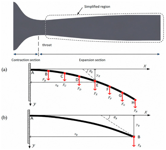
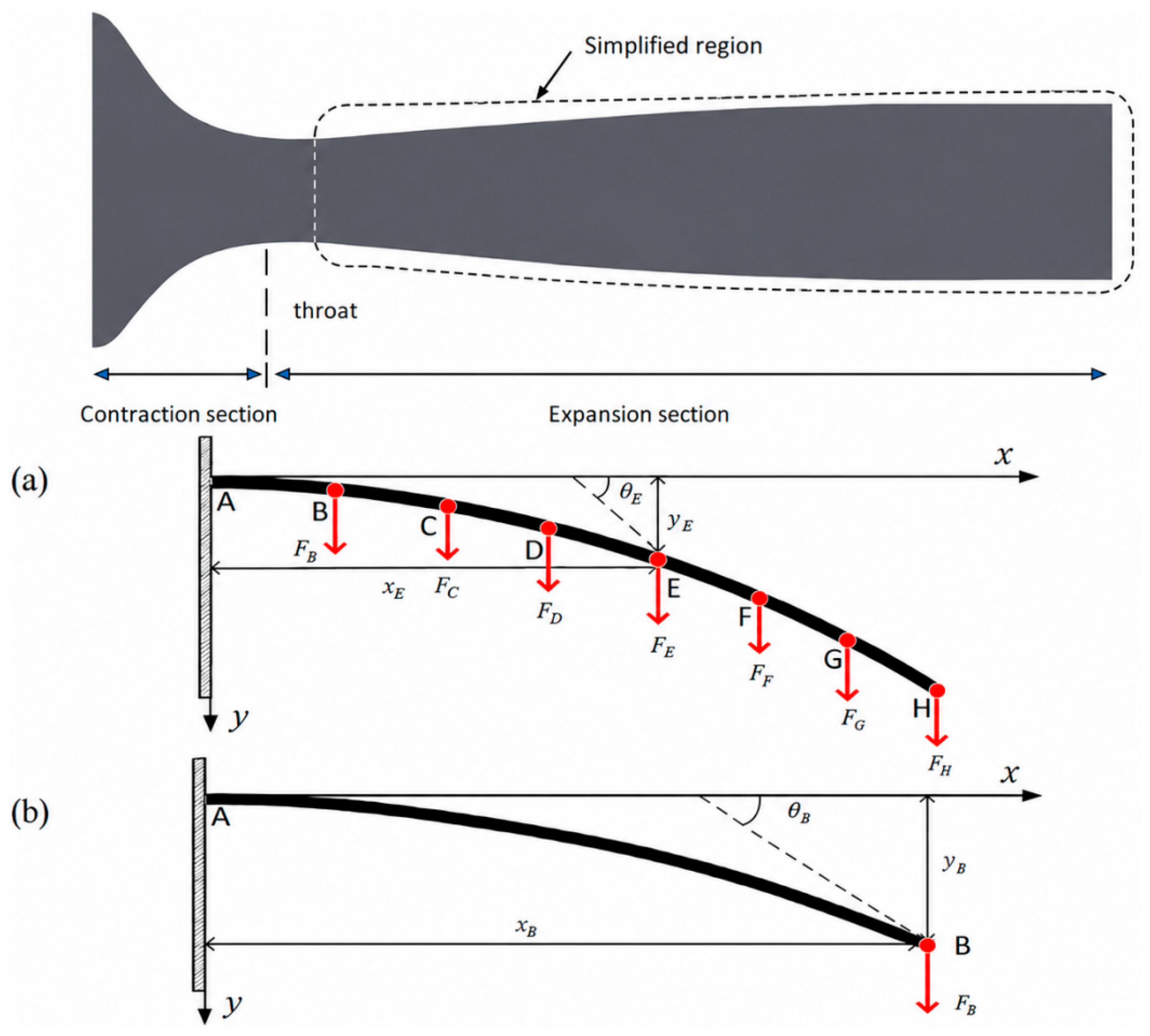
As shown in Figure 1, the jet nozzle can be structurally divided into three sections: the subsonic section, the throat section, and the supersonic section. Depending on the operating conditions of the nozzle, airflow at different Mach numbers requires acceleration treatment. To meet practical needs, the nozzle profile is typically controlled by hydraulic actuators. Thus, nozzles can be further categorized into fully flexible nozzles (where all three sections are hydraulically controlled) and semi-flexible nozzles (where the subsonic section is rigid, while the throat and supersonic sections are hydraulically controlled). Compared to fully flexible nozzles, semi-flexible nozzles have gained broader application due to their simpler control systems and lower manufacturing costs. Therefore, this paper focuses on developing a mechanistic model for semi-flexible nozzles.

Figure 1. Schematic of the flexible nozzle and its simplified beam model: (a) multi-pivot beam model; (b) definitions of the transverse deflection y_B and tangent rotation angle θ_B at point B.

The aerodynamic reference profiles corresponding to the considered Mach number commands are prescribed offline and treated as known inputs to the multi-pivot control system. These profiles are assumed to have been generated during the aerodynamic design stage using established supersonic-nozzle design approaches, such as the method of characteristics. The present control-oriented model focuses on the structural deformation and tracking of the prescribed profiles and does not explicitly include the internal shock-wave dynamics in the nozzle diverging section. Under this assumption, the nozzle expansion section is taken as the research object. The coordinate system is established at the fixed point of the expansion section. Seven load points are uniformly distributed along the expansion section, and each load point is driven by a hydraulic actuator.

The nozzle expansion section is taken as the research object. The coordinate system is set at the fixed point of the expansion section. Seven load points are uniformly distributed along the length of the expansion section, each controlled by a hydraulic actuator. It is important to note that the thickness of the nozzle’s flexible wall is negligible compared to its width and length. This allows the assumption that the expansion section can be modeled as a flexible shell. Furthermore, the effects of warping and lateral shear can be disregarded since the forced displacement of the flexible shell is uniform across its width. Therefore, the mechanical model of the nozzle flexible wall profile will be equivalent to an Euler beam. The analytical solution is calculated using beam deformation theory and corrected using the strain–moment relationship of flexible shells. As shown in Figure 1a,b, simplifying the flexible wall of the nozzle expansion section into a beam mechanical model provides a reasonable simplification for subsequent theoretical analysis.

For ease of derivation, we first analyze the single-support case, as shown in Figure 1b. A cantilever beam model is fixed at point A, with a vertical downward force $F_B$ applied at point B, causing the AB segment to bend. At point B, where $x_B=a$, the transverse deflection is denoted by $y_B=y\left(a\right)$. The deflection angle ${\theta }_B$ is defined as the rotation of the tangent to the deformed beam centerline at point B relative to the undeformed beam axis, as illustrated in Figure 1b. Therefore,

$${\theta }_B=\arctan \left({\left.{\displaystyle \frac{dy}{dx}}\right|}_{x=a}\right)$$

(3)

Under the small-slope assumption $\left|dy/dx\right|\ll 1$, the deflection angle can be approximated as

$${\theta }_B\approx {\left.{\displaystyle \frac{dy}{dx}}\right|}_{x=a}$$

(4)

Given that $x_B=a$, the curvature moment equation and the curvature equation of the curve yield the following system of equations:

$$\left\{\begin{array}{l}{\displaystyle \frac{1}{R}}={\displaystyle \frac{M(x)}{EI}}\\ {\displaystyle \frac{1}{R}}={\displaystyle \frac{\frac{d^{2}y}{d{x}^2}}{{[1+{(\frac{dy}{dx})}^2]}^{\frac{3}{2}}}}\end{array}\right.$$

(5)

where $x$ is the horizontal position of the surface, $y$ is the corresponding deflection, $dy/dx$ is the rate of change in deflection, $R$ is the radius of curvature, $1/R$ is the curvature, $M(x)$ is the bending moment, $E$ is the elastic modulus, and $I$ is the sectional moment of inertia. In practice, the rate of change at any single point is very small (far less than 1, i.e., $dy/dx\ll 1$), so the above equation can be simplified to:

$${\displaystyle \frac{d^{2}y}{d{x}^2}}={\displaystyle \frac{M(x)}{EI}}$$

(6)

For flexible wall panels, based on the cantilever beam model assumption, the strain along the beam between each support point exhibits a linear distribution along the axis. Therefore, the bending moment at any point before segment AB is:

$$M(x)=-F_B(a-x)$$

(7)

In actual operating conditions, since the exit section of the supersonic portion of the nozzle is fixed within the instrument, the boundary conditions during the control process can be considered as having both displacement and shape change in the exit section equal to zero. Therefore, the boundary condition is: $y(0)=0;y^{\prime }(0)=0$. Based on the simplified curvature bending moment equation and the boundary condition, the analytical solution of the equation can be derived:

$$\left\{\begin{array}{l}{\displaystyle \frac{dy}{dx}}={\displaystyle \frac{-F_B}{EI}}(ax-{\displaystyle \frac{x^2}{2}})\\ y={\displaystyle \frac{-F_B{x}^2}{6EI}}(3a-x)\end{array}\right.$$

(8)

It should be noted that when $x$ is beyond point $B$, the beam arm model will no longer be subjected to force $F$. At this point, the boundary conditions at the load point $B$ must be considered:

$$\left\{\begin{array}{l}{\displaystyle \frac{dy}{dx}}{|}_{x=a}={\displaystyle \frac{-F_B{a}^2}{2EI}}\\ y(a)={\displaystyle \frac{-F_B{a}^3}{3EI}}\end{array}\right.$$

(9)

Based on the boundary conditions at point $B$, the equations for all subsequent $x$ values can be derived. Using the deflection at point $B$, the corresponding analytical solutions can be determined:

$$\left\{\begin{array}{l}{\displaystyle \frac{dy}{dx}}={\displaystyle \frac{-F_B{a}^2}{2EI}}\\ y={\displaystyle \frac{-F_B{a}^2}{6EI}}(3x-a)\end{array}\right.$$

(10)

Combining the above equations, the mathematical equation for the flexible wall of the nozzle expansion section at a single pivot point $B$ can be written as:

$$\left\{\begin{array}{l}y={\displaystyle \frac{-F_B{x}^2}{6EI}}(3a-x) if 0\le x<a\\ y={\displaystyle \frac{-F_B{a}^2}{6EI}}(3x-a) if x\ge a\end{array}\right.$$

(11)

In summary, based on the principle of superposition of forces at multiple points, the mathematical equation for the flexible wall deformation of a nozzle subjected to multi-point forces can be extended as follows:

$$\left\{\begin{array}{l}{y}_{F_i,x,j}={\displaystyle \sum _{i=1}^7\frac{F_i{x}^2}{6EI}}({\displaystyle \frac{i}{N}}3a_j-x) if 0\le x<a_j\\ y_{F_i,x,j}={\displaystyle \sum _{i=1}^7\frac{F_i{a_j}^2}{6EI}}({\displaystyle \frac{i}{N}}3x-a_j) if x\ge a_j\end{array}\right.$$

(12)

3. The Air Intake Subsystem Model

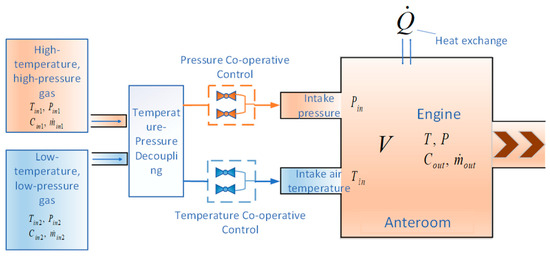
The intake system structure diagram for this paper is shown in Figure 2. First, the intake system receives gas supply from the mixer, which provides both high-temperature/high-pressure and low-temperature/low-pressure gases. Since the input gases are coupled in terms of temperature and pressure, a temperature–pressure decoupling stage is incorporated to precisely control the temperature and pressure of the flow entering the engine. Subsequently, the intake system employs two sets of control valves (each set comprising a butterfly valve and a plunger valve) to independently regulate temperature and pressure. To ensure system functionality under exceptional conditions (e.g., unexpected valve failure), the valve controller design employs dual-valve cooperative control. This dual-valve configuration jointly maintains stable operation of the intake system, providing consistent operating conditions for subsequent jet nozzle simulation.

Figure 2. Intake system structure diagram.

3.1. Intake Chamber Model

The intake system can be simplified as a two-inlet, one-outlet volumetric model, where $T_{in1},P_{in1},{\dot{m}}_{in1},C_{in1},h_{in1}$ represent the temperature, pressure, mass flow rate, average flow velocity, and enthalpy of the high-temperature, high-pressure intake air, respectively; $T_{in2},P_{in2},{\dot{m}}_{in2},C_{in2},h_{in2}$ respectively denote the temperature, pressure, mass flow rate, average flow velocity, and enthalpy of the inlet air in the low-temperature, low-pressure intake system; $T,P,C,h,{\dot{m}}_{eng}$ at the chamber outlet represent the equivalent exhaust temperature, pressure, average flow velocity, enthalpy, and mass flow rate.

The original lumped-parameter model assumes ideal and instantaneous mixing. However, practical gas-mixing systems are affected by incomplete mixing, energy losses, flow non-uniformity, and thermal inertia, resulting in deviations between the actual and theoretical outlet states [13]. Similar non-ideal mixing-chamber models introduce an effective mixing-efficiency coefficient to characterize these effects [14]. Therefore, an effective energy-transfer efficiency coefficient ${\eta }_i$ is introduced for each inlet stream, where i = 1, 2 and $0<{\eta }_i\le 1$. The effective inlet energy flux is expressed as

$${\dot{E}}_{in}={\displaystyle \sum _{i=1}^2{\eta }_i\left(h_{in,i}+\frac{C_{in,i}^2}{2}\right)}{\dot{m}}_{in,i}$$

(13)

When ${\eta }_i=1$, the model reduces to the ideal chamber model. A value lower than unity represents the combined effects of incomplete mixing, heat-transfer losses, and other unmodelled flow losses. The efficiency coefficients are selected according to the reported range in the literature, and their influence is evaluated through sensitivity analysis.

Based on mass conservation, energy conservation, and the ideal-gas law, the pressure and temperature dynamics of the intake chamber can be derived as follows [15]:

$$\begin{array}{ll}{\displaystyle \frac{dP}{dt}}& ={\displaystyle \frac{R}{V}}\left[\left(T-{\displaystyle \frac{\left(h-RT\right)}{\left(c_p-R\right)}}\right)\left({\dot{m}}_{in1}+{\dot{m}}_{in2}-{\dot{m}}_{out}\right)\right]\\ & +{\displaystyle \frac{R}{V\left(c_p-R\right)}}\left[{\eta }_1\left(h_{in1}+{\displaystyle \frac{C_{in1}^2}{2}}\right){\dot{m}}_{in1}+{\eta }_2\left(h_{in2}+{\displaystyle \frac{C_{in2}^2}{2}}\right){\dot{m}}_{in2}+\dot{Q}-\left(h+{\displaystyle \frac{C_{out}^2}{2}}\right){\dot{m}}_{out}\right]\end{array}$$

(14)

$$\begin{array}{ll}{\displaystyle \frac{dT}{dt}}& ={\displaystyle \frac{RT}{pV\left(c_p-R\right)}}\left[-\left({\dot{m}}_{in1}+{\dot{m}}_{in2}-{\dot{m}}_{out}\right)\left(h-RT\right)+\dot{Q}\right]\\ & +{\displaystyle \frac{RT}{pV\left(c_p-R\right)}}\left[{\eta }_1\left(h_{in1}+{\displaystyle \frac{C_{in1}^2}{2}}\right){\dot{m}}_{in1}+{\eta }_2\left(h_{in2}+{\displaystyle \frac{C_{in2}^2}{2}}\right){\dot{m}}_{in2}-\left(h+{\displaystyle \frac{C_{out}^2}{2}}\right){\dot{m}}_{out}\right]\end{array}$$

(15)

where $c_p$ is the specific heat capacity of the gas at constant pressure within the chamber; $R$ is the gas constant for air; $Q$ is the total heat exchanged between the chamber and the external environment; $V$ represents the volume of the equivalent chamber in the intake system. ${\eta }_1$ and ${\eta }_2$ denote the respective effective energy-transfer efficiencies of the high-temperature, high-pressure inlet stream and the low-temperature, low-pressure inlet stream.

3.2. Intake System Valve Model

The temperature and pressure within the intake plenum are jointly controlled by a set of plunger valves and butterfly valves. According to relevant literature research, these butterfly valves and plunger valves can effectively be simplified as inertial elements. The actuator dynamics of the butterfly valve are approximated by a stable first-order inertial model [16]:

$$\dot{\phi }={\displaystyle \frac{-\phi +k_{\phi }{u}_1}{T_{\phi }}}$$

(16)

where $\phi$ represents the valve opening; $k_{\phi }$ and $T_{\phi }$ denote the actuator gain and time constant, respectively; $u_1$ is the corresponding control input. The motion model of a plunger valve can be simplified to a two-stage inertial system, with the common motion equation being:

$$\ddot{\phi }=-2\zeta \omega \dot{\phi }-{\omega }^2\phi +{\omega }^2{u}_2$$

(17)

where $\zeta$ is the damping ratio; $\omega$ is the undamped oscillation frequency; $u_2$ is the control rate of the plunger valve. Additionally, the relationship between the valve opening $\phi$ and the mass flow rate $W$ through the valve can be expressed as follows, where $\phi$ is expressed as a percentage and satisfies $\phi \in \left[0,100\right]\%$:

$$W=\lambda s\sqrt{2\rho \cdot \mathrm{\Delta }p}$$

(18)

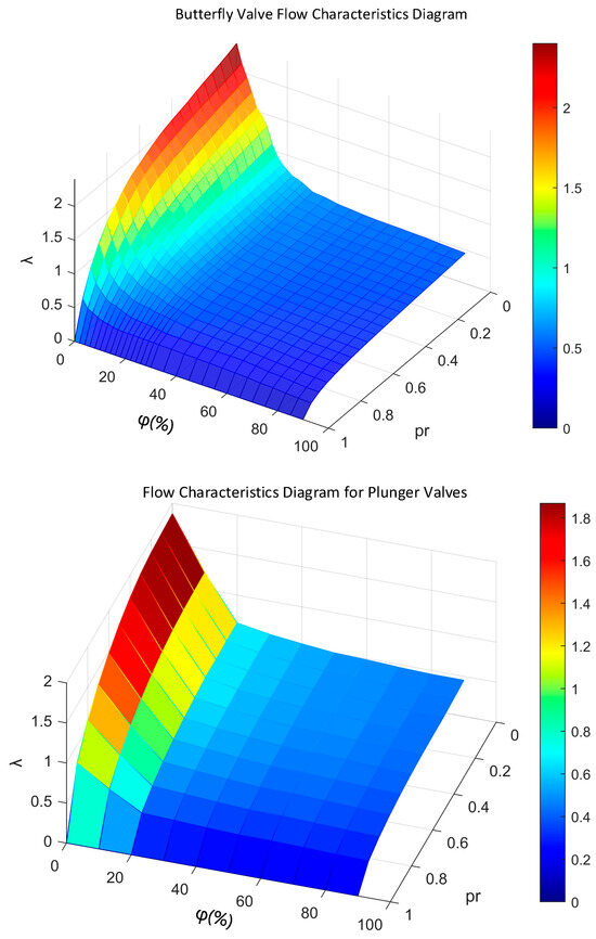
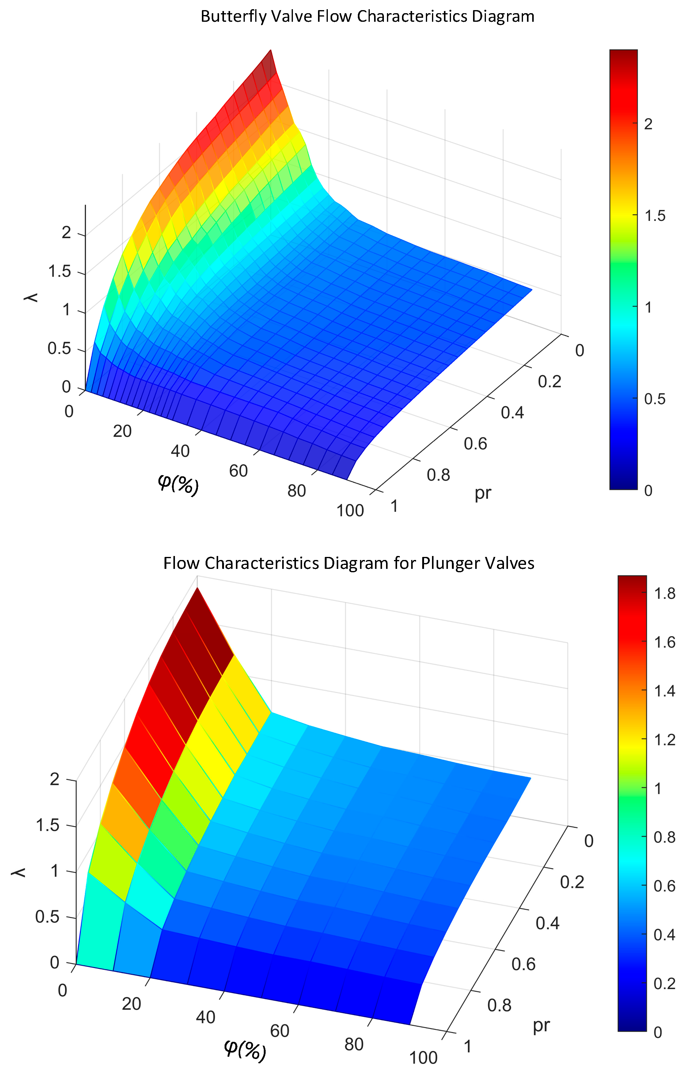
In the formula, $s$ represents the flow area of the valve; $\rho$ denotes the density of the gas flowing through the valve; $\mathrm{\Delta }p$ is the pressure difference across the valve; $\lambda$ is the flow coefficient of the valve, which varies for different valve types, as shown in Figure 3:

Figure 3. Flow characteristics of the butterfly valve and plunger valve as functions of valve opening and pressure ratio.

4. Design of Composite Controllers

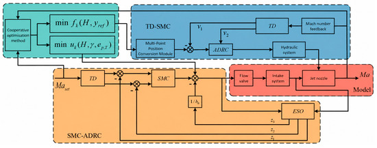
The control of a multi-pivot semi-flexible nozzle system primarily comprises two components: inlet temperature and pressure control, and multi-pivot cooperative control. The former regulates the temperature and pressure entering the nozzle via a cooperative controller, while the latter controls the pivot positions to alter the nozzle’s profile. These two components work in tandem to maximize tracking of the desired Mach number command. The system control structure is illustrated in Figure 4. The proposed control system consists of three interconnected layers. First, the multi-pivot allocation layer calculates the force commands required to reproduce the reference nozzle profile. Second, the intake control layer regulates the pressure and temperature through pressure–temperature decoupling, cooperative valve allocation, and SMC-LADRC. Third, the outer loop generates a correction term from the Mach number tracking error and updates the inner-loop reference commands. The following subsections present the design and analysis of these three layers in sequence.

Figure 4. System control structure diagram.

4.1. Multi-Point Control

4.1.1. Multi-Point Collaborative Algorithm

For multi-support systems, multiple support points are uniformly distributed across the flexible nozzle surface. By applying different forces $f$ at these support points, the nozzle profile is altered, and its position $y_{ref}$ is adjusted via a hydraulic press. Therefore, designing an algorithm to determine the force f at each support point and control the hydraulic actuators to track the prescribed Mach-number-dependent reference profile. The reference profile $y_{\mathrm{ref}}\left(x,M_{\mathrm{ref}}\right)$ is generated offline and supplied to the cooperative force-allocation algorithm as a known command.

The mathematical expression for the flexible nozzle profile was obtained in Section 2, namely Equation (12). Based on this, the flexibility matrix $H$ was designed:

$$\left\{\begin{array}{l}H=\left[\begin{array}{ccc}h(x_1,p_1)& \dots & h(x_1,p_m)\\ ⋮& \ddots & ⋮\\ h(x_n,p_1)& \dots & h(x_n,p_m)\end{array}\right],\\ h(x,p)=\left\{\begin{array}{ll}-{\displaystyle \frac{p^2}{6EI}}(3x-p)& x>p\\ -{\displaystyle \frac{x^2}{6EI}}(3p-x)& x\le p\end{array}\right.\end{array}\right.$$

(19)

where $x_n$ denotes the position at the $n$th location of the nozzle; $p_m$ denotes the position of the $m$th pivot point. Since the matrix contains unit stresses, $f=1$. Based on the flexibility matrix $H$, formulate the constrained optimization problem:

$$\begin{array}{cc}\hfill \underset{f}{\min }& {\displaystyle \frac{1}{2}}{\Vert Hf-y_{ref}\Vert }_2^2\hfill \\ \hfill \mathrm{s}.\mathrm{t}.& f_{\min }\le f_i\le f_{\max } (i=1,2,\dots ,m)\hfill \end{array}$$

(20)

For this optimization problem with inequality constraints, we design KKT optimality conditions and construct the Lagrange function:

$$\begin{array}{cc}\hfill \underset{f}{\min }& J(f)={\displaystyle \frac{1}{2}}{f}^T(H^{T}H)f-{(H^T{y}_{ref})}^{T}f\hfill \\ \hfill \mathrm{s}.\mathrm{t}.& g_i^L(f)=f_{\min }-f\le 0, i=1,2,\dots ,m\hfill \\ \hfill & h_i^U(f)=f_i-f_{\max }\le 0, i=1,2,\dots ,m\hfill \end{array}$$

(21)

$$L(f,\lambda ,\mu )=J(f)+{\displaystyle {\displaystyle \sum _{i=1}^m}{\lambda }_i^L{g}_i^L(f)}+{\displaystyle {\displaystyle \sum _{i=1}^m}{\mu }_i^U{h}_i^U(f)}, {\lambda }_i^L\ge 0,{\mu }_i^U\ge 0.$$

(22)

Construct complementary slack conditions based on actual physical constraints:

$$\left\{\begin{array}{l}{\lambda }_i^L(f^{*}-f_{\min })=0\\ {\mu }_i^U(f_{\max }-f^{*})=0\end{array}\right.$$

(23)

In summary, by differentiating the Lagrangian function and incorporating the complementary slack conditions, the Karush–Kuhn–Tucker conditions of problem (20) are therefore obtained as:

$$\left\{\begin{array}{l}J(f^{*})+{\displaystyle {\displaystyle \sum _{i=1}^m}{\lambda }_i^L\nabla g_i^L(f^{*})}+{\displaystyle {\displaystyle \sum _{i=1}^m}{\mu }_i^U\nabla h_i^U(f^{*})}=0\\ {\lambda }_i^L(f^{*}-f_{\min })=0\\ {\mu }_i^L(f_{\max }-f^{*})=0\\ {\lambda }_i^L\ge 0,{\mu }_i^L\ge 0\\ f_{\min }\le f_i\le f_{\max }\end{array}\right.$$

(24)

Since problem (20) is a convex quadratic program and the feasible set is nonempty and convex, the KKT conditions are necessary and sufficient for global optimality. In the online implementation, the optimal force vector is obtained using the projected-gradient iteration introduced in Section 4.1.2.

4.1.2. Convergence Proof of the Cooperative Optimization Algorithm

Define the feasible set as

$$\Omega =\left\{f\in {ℝ}^m|f_{\min }\le f_i\le f_{\max }, i=1,\dots ,m\right\}$$

(25)

The objective function in (20) is written as

$$J(f)={\displaystyle \frac{1}{2}}{‖Hf-y_{\mathrm{ref}}‖}_2^2$$

(26)

The corresponding projected-gradient iteration is

$$f_{k+1}=P_{\Omega }\left[f_k-\alpha \nabla J(f_k)\right]$$

(27)

where $P_{\Omega }\left(\cdot \right)$ denotes the Euclidean projection onto Ω, and α > 0 is the iteration step size.

Lemma 1.

For any nonempty closed convex set Ω, the Euclidean projection operator $P_{\Omega }\left(\cdot \right)$ is nonexpansive, i.e.,

$${‖P_{\Omega }\left(x\right)-P_{\Omega }\left(y\right)‖}_2\le {‖x-y‖}_2$$

(28)

This standard property of convex projection can be found in the convex optimization literature [17].

For the quadratic objective function $J(f)$, its gradient is

$$\nabla J(f)=H^{\mathrm{T}}\left(Hf-y_{\mathrm{ref}}\right)$$

(29)

Therefore, for any $f,g\in {ℝ}^m$,

$$\begin{array}{ll}{‖\nabla J(f)-\nabla J(g)‖}_2& ={‖H^{\mathrm{T}}H(f-g)‖}_2\\ & \le {‖H^{\mathrm{T}}H‖}_2{‖f-g‖}_2\end{array}$$

(30)

Hence, $\nabla J$ is Lipschitz continuous with

$$L={‖H^{\mathrm{T}}H‖}_2={\lambda }_{\max }\left(H^{\mathrm{T}}H\right)$$

(31)

Lemma 2.

A feasible point $f^{*}\in \Omega$ is an optimal solution of problem (20) if and only if, for any α > 0,

$$f^{*}={{\rm P}}_{\Omega }(f^{*}-\alpha \nabla J(f^{*})), \forall \alpha >0$$

(32)

This projected fixed-point characterization follows from the first-order optimality condition for constrained convex optimization [17].

Lemma 3

[18]. If $H$ has full column rank, then

$$\mu ={\lambda }_{\min }\left(H^{\mathrm{T}}H\right)>0$$

(33)

and the gradient of J is strongly monotone:

$${\left(f-g\right)}^{\mathrm{T}}\left[\nabla J(f)-\nabla J(g)\right]\ge \mu {‖f-g‖}_2^2$$

(34)

The above lemmas collectively establish the convergence of formula (20). The specific proof proceeds as follows: First, we demonstrate the global convergence of the objective function. Subsequently, we prove linear-rate convergence under strong convexity conditions. The detailed proof is outlined below:

Proof. 

Proof of global convergence:

Using the projected gradient method, define the iteration point: $g_k=f_k-\alpha \nabla J(f_k)$, $g^{*}=f^{*}-\alpha \nabla J(f^{*})$. By Lemmas 1 and 3, we obtain:

$$\Vert f_{k+1}-f^{*}\Vert =\Vert {{\rm P}}_{\Omega }(g_k)-{{\rm P}}_{\Omega }(g^{*})\Vert \le \Vert g_k-g^{*}\Vert =\Vert (f_k-f^{*})-\alpha (\nabla J(f_k)-\nabla J(f^{*}))\Vert$$

(35)

Take the square of the norm:

$$\begin{array}{ll}{\Vert g_k-g^{*}\Vert }^2=& {\Vert f_{k+1}-f^{*}\Vert }^2-2\alpha {(f_k-f^{*})}^T(\nabla J(f_k)-\nabla J(f^{*}))\\ & +{\alpha }^2{\Vert \nabla J(f_k)-\nabla J(f^{*})\Vert }^2\end{array}$$

(36)

According to the properties of convex functions (gradient monotonicity):

$${(f_k-f^{*})}^T(\nabla J(f_k)-\nabla J(f^{*}))\ge {\displaystyle \frac{1}{L}}{\Vert \nabla J(f_k)-\nabla J(f^{*})\Vert }^2$$

(37)

Substituting Equation (9) into (8) yields:

$${\Vert g_k-g^{*}\Vert }^2\le {\Vert f_k-f^{*}\Vert }^2-\alpha ({\displaystyle \frac{2}{L}}-\alpha ){\Vert \nabla J(f_k)-\nabla J(f^{*})\Vert }^2$$

(38)

When $0<\alpha <{\displaystyle \frac{2}{L}}, {\displaystyle \frac{2}{L}}-\alpha >0$:

$${\Vert f_{k+1}-f^{*}\Vert }^2\le {\Vert f_k-f^{*}\Vert }^2-c{\Vert \nabla J(f_k)-\nabla J(f^{*})\Vert }^2$$

(39)

When $c=\alpha ({\displaystyle \frac{2}{L}}-\alpha )>0$, the sequence $\Vert f_k-f^{*}\Vert$ is monotonically decreasing and has a lower bound; hence, it converges. Furthermore, ${\displaystyle \sum _{k=0}^{\infty }{\Vert \nabla J(f_k)-\nabla J(f^{*})\Vert }^2}<{\displaystyle \frac{1}{c}}{\Vert f_0-f^{*}\Vert }^2<\infty$ implies $\underset{k\to \infty }{\lim }\Vert \nabla J(f_k)-\nabla J(f^{*})\Vert =0$. By virtue of the properties of convex functions and the closed convexity of the feasible region, this sequence converges to the optimal solution. □

Proof. 

Proof of linear convergence for strongly convex cases:

By applying Lemma 3:

$${(f_k-f^{*})}^T(\nabla J(f_k)-\nabla J(f^{*}))\ge \mu {\Vert f_k-f^{*}\Vert }^2$$

(40)

Combining the strong-monotonicity inequality in (40) with the Lipschitz bound in (30) and the error recursion in (36) yields:

$$\Vert f_{k+1}-f^{*}\Vert \le (1-2\alpha \mu +{\alpha }^2{L}^2)\Vert f_k-f^{*}\Vert$$

(41)

Let ${\rho }^2=1-2\alpha \mu +{\alpha }^2{L}^2$. When $0<\alpha <2/L$ and $\mu >0$, the minimum value is attained at $\alpha =\mu /L^2$, where ${\rho }_{\min }^2=1-{\mu }^2/L^2<1$. Since $\rho <1$, linear convergence holds. □

4.1.3. Servo System Controller

Position error feedback control based on the ADRC framework is employed for the nozzle position $y$. Data interpolation using corresponding nozzle profile data for different Mach numbers yields a series of reference position signal points $y_{ref}$ for the nozzle profile as Mach number varies. Damping coupling of the hydraulic actuator model while retaining elastic terms simplifies it to a second-order model:

$$m\ddot{x}+n\dot{x}+kx=bu$$

(42)

To design the ADRC controller, the model was rewritten as follows:

$$\left\{\begin{array}{l}{x}_1=y,x_2=\dot{y}\\ {\dot{x}}_1=x_2\\ {\dot{x}}_2=-{\displaystyle \frac{n}{m}}{x}_2-{\displaystyle \frac{k}{m}}{x}_1+{\displaystyle \frac{b}{m}}u+d(t)\end{array}\right.$$

(43)

where $m,n,k,b$ denote the model parameters; $d(t)$ represents the total disturbance arising from the combination of parameter uncertainty and external disturbances. The ESO is designed based on the system model:

$$\left\{\begin{array}{l}{\dot{\widehat{x}}}_1={\widehat{x}}_2+{\beta }_1(y-{\widehat{x}}_1)\\ {\dot{\widehat{x}}}_2={\widehat{x}}_3-{\displaystyle \frac{n}{m}}{\widehat{x}}_2-{\displaystyle \frac{k}{m}}{\widehat{x}}_1+{\displaystyle \frac{b}{m}}u+{\beta }_2(y-{\widehat{x}}_1)\\ {\dot{\widehat{x}}}_3={\beta }_3(y-{\widehat{x}}_1)\end{array}\right.$$

(44)

where ${\widehat{x}}_1,{\widehat{x}}_2,{\widehat{x}}_3$ denote the observed values of $x_1,x_2,d(t)$; ${\beta }_1,{\beta }_2,{\beta }_3$ represent the observed parameters of the ESO. The control rate $u_y$ for the fulcrum position of the hydraulic actuator is designed as follows:

$$\left\{\begin{array}{l}{\epsilon }_1=y-y_{ref},{\epsilon }_2=\dot{y}\\ u_y={\displaystyle \frac{m}{b}}(-k_1{\epsilon }_1-k_2{\epsilon }_2-{\widehat{x}}_3)\end{array}\right.$$

(45)

where $k_1,k_2$ are parameters of the controller; substituting the control rate $u_y$ into the system equations yields:

$$\begin{array}{ll}{\dot{\epsilon }}_2& =-{\displaystyle \frac{n}{m}}{\epsilon }_2-{\displaystyle \frac{k}{m}}{\epsilon }_1+{\displaystyle \frac{b}{m}}u+d(t)\\ & =-\underset{a_2}{\underbrace{({\displaystyle \frac{n}{m}}+k_2)}}{\epsilon }_2-\underset{a_1}{\underbrace{({\displaystyle \frac{k}{m}}+k_1)}}{\epsilon }_1+\underset{\delta (t)}{\underbrace{(d(t)-{\widehat{x}}_3)}}\end{array}$$

(46)

The complete closed-loop error dynamics can be written as:

$$\left\{\begin{array}{l}{\dot{\epsilon }}_1={\epsilon }_2\\ {\dot{\epsilon }}_2=-a_2{\epsilon }_2-a_1{\epsilon }_1+\delta (t)\end{array}\right.$$

(47)

When the ESO observations can compensate for the total disturbance, i.e., $\delta (t)\approx 0$, the expected closed-loop characteristic equation yields:

$$p^2+2\zeta {\omega }_{n}p+{\omega }_n^2=0\equiv p^2+({\displaystyle \frac{n}{m}}+k_2)p+({\displaystyle \frac{k}{m}}+k_1)$$

(48)

where ${\omega }_n$ denotes the natural frequency and $\zeta$ represents the damping ratio. The controller parameters may be determined as follows:

$$k_1={\omega }_n^2-{\displaystyle \frac{k}{m}}, k_2=2\zeta {\omega }_n-{\displaystyle \frac{n}{m}}$$

4.1.4. Stability Analysis of the Servo System

Define the observer estimation errors as $e_1=x_1-{\widehat{x}}_1,e_2=x_2-{\widehat{x}}_2,e_3=d-{\widehat{x}}_3$. $d\left(t\right)$ is the lumped disturbance. Subtracting the observer dynamics in (44) from the plant dynamics in (43) gives:

$$\underset{\dot{e}}{\underbrace{\left[\begin{array}{l}{\dot{e}}_1\\ {\dot{e}}_2\\ {\dot{e}}_3\end{array}\right]}}=\underset{A_{eso}}{\underbrace{\left[\begin{array}{ccc}-{\beta }_1& 1& 0\\ -{\beta }_2& -{\displaystyle \frac{n}{m}}& 1\\ -{\beta }_3& 0& 0\end{array}\right]}}\left[\begin{array}{l}{e}_1\\ e_2\\ e_3\end{array}\right]+\underset{w(t)}{\underbrace{\left[\begin{array}{c}0\\ 0\\ \dot{d}(t)\end{array}\right]}}$$

(49)

Construct a Lyapunov function $V_e=e^T{P}_{e}e$, satisfying the condition:

$$A_{eso}^T{P}_e+P_e{A}_{eso}=-Q_e$$

(50)

where both $P_e$ and $Q$ are symmetric positive definite matrices, differentiating with respect to $V_e$ yields:

$${\dot{V}}_e=-e^T{Q}_{e}e+2e^T{P}_{e}w(t)\le -{\lambda }_{e,\min }(Q_e){\Vert e\Vert }^2+2\Vert P_e\Vert \cdot \Vert e\Vert \cdot \Vert \dot{d}\Vert$$

(51)

Here, ${\lambda }_{e,\min }(Q_e)$ denotes the smallest eigenvalue of matrix $Q_e$. Since $Q_e$ is positive definite, ${\lambda }_{e,\min }(Q_e)>0$.

By standard ISS theory [19,20], the exponential function $e(t)$ converges to an interval proportional to $\sup |\dot{d}|$:

$$\Vert e(t)\Vert \le c_1{e}^{-\gamma t}\Vert e(0)\Vert +c_2\underset{0\le \tau \le t}{\sup }|\dot{d}(\tau )|$$

(52)

where $c_1>0,c_2>0,\gamma >0$. Thus $\delta (t)=e_3(t)$ also exhibits the same decay trend with a small residual component. Similarly, for the closed-loop error dynamics in (47) of the main control system, a quadratic Lyapunov function $V_{\epsilon }={\epsilon }^T{P}_{\epsilon }\epsilon$ may be designed. Taking the derivative with respect to $V_{\epsilon }$ and applying standard ISS theory, we derive:

$$\Vert \epsilon (t)\Vert \le c_3{\epsilon }^{-\eta t}\Vert \epsilon (0)\Vert +c_4\underset{0\le \tau \le t}{\sup }|\delta (\tau )|$$

(53)

where $c_3>0,c_4>0,\eta >0$. Combining the observer-error bound in (52) and the tracking-error bound in (53), the final error satisfies the following condition:

$$\underset{t\to \infty }{\lim \sup }\Vert \epsilon (t)\Vert \le c_4\underset{t\to \infty }{\lim \sup }\Vert \delta (t)\Vert \le c_4(c_2|\dot{d}|)$$

(54)

Therefore, under bounded disturbance variations, the observer and tracking errors are uniformly ultimately bounded. The size of the residual set depends on the disturbance-derivative bound and the selected observer and controller gains.

4.2. Intake Co-Operative Control

4.2.1. Dual-Valve Cooperative Fault-Tolerance Algorithm

The stable operation of the air intake system is a prerequisite for the jet nozzle to maintain stable tracking of a given Mach number. However, given that the intake system is controlled by multiple valves of different types and considering the complexity of the operating conditions it encounters, it is essential to ensure the system’s stable operation even in the event of valve failure. According to the intake-chamber model in (14) and (15), the cavity model can be expressed in the following affine form:

$$\left\{\begin{array}{l}\dot{P}=f_P(T)+b_{11}(T){\varphi }_1+b_{12}(T){\varphi }_2\\ \dot{T}=f_T(P,T)+b_{21}(P,T){\varphi }_1+b_{22}(P,T){\varphi }_2\end{array}\right.$$

(55)

where $f_P(T),f_T(P,T)$ represent disturbance terms for intake system pressure and temperature; $b_{11}(T),b_{12}(T),b_{21}(P,T),b_{22}(P,T)$ denote the coupling matrix; and ${\varphi }_1,{\varphi }_2$ indicate valve opening, which in this study was obtained through interpolation of actual test data.

The intake plenum system constitutes a complex temperature–pressure coupled model. To simplify control, preliminary processing is required to decouple temperature and pressure inputs from the plenum model. Temperature control and pressure control are subsequently decoupled onto separate intake channels, achieving coordinated control through dual-valve operation; decoupling design for a four-valve dual-input plenum system may be implemented as follows:

$$\tilde{U}=BU$$

(56)

where $U={[u_1,u_2]}^T$ denotes the input demand equivalent control rate; $\tilde{U}={[U_P,U_T]}^T$ represents the decoupled virtual control variable. For dual-input cavity models, as the first input comprises high-temperature, high-pressure gas while the second comprises low-temperature, low-pressure gas, their effects on cavity temperature and pressure are mathematically non-redundant—that is, reversible. Thus, the actual valve control rate may be determined via $U=B^{-1}\tilde{U}$.

Following decoupling, the equivalent input demand is determined, and the control rate is then allocated to specific butterfly valves and plunger valves through collaborative optimization. The secondary planning cost function is designed as follows:

$$J(u,e_P,e_T)={\displaystyle \frac{1}{2}}{u}^{T}Hu+{\gamma }_1{e}_P^2+{\gamma }_2{e}_T^2$$

(57)

where $u=[u_{11},u_{12};u_{21},u_{22}]$ represents the valve control variable; $H=[a_{11},a_{12};a_{21},a_{22}]$ denotes the energy consumption coefficient matrix; ${\gamma }_1{e}_P^2,{\gamma }_2{e}_T^2$ signifies the error penalty term. The design ensures that the convex matrix $H$ is a positive definite matrix. Considering physical boundary constraints and control equivalence, the following optimization problem is formulated:

$$\begin{array}{ll}\underset{u}{\min }& {\displaystyle \frac{1}{2}}{u}^{T}Hu+{\gamma }_1{e}_P^2+{\gamma }_2{e}_T^2\\ & s.t. \alpha =k_{11}{u}_{11}+k_{12}{u}_{12}-u_1,\\ & \beta =k_{21}{u}_{21}+k_{22}{u}_{22}-u_2,\\ & g_i^L(u)=0-u_i\le 0, i=1,2,\\ & h_i^U(u)=u_i-{\overline{u}}_i\le 0, i=1,2.\end{array}$$

(58)

Construct the Lagrangian function for optimization problem (58):

$$\mathcal{L}={\displaystyle \frac{1}{2}}{u}^{T}Hu+{\gamma }_1{e}_P^2+{\gamma }_2{e}_T^2+{\lambda }_1\alpha +{\lambda }_2\beta +{\displaystyle {\displaystyle \sum _{i,j=1}^2}{\xi }_{ij}^L{g}_i^L(u)+}{\displaystyle {\displaystyle \sum _{i,j=1}^2}{\zeta }_{ij}^U{h}_i^U(u)}$$

(59)

where ${\xi }_{ij}^L\ge 0,{\zeta }_{ij}^U\ge 0, \forall i,j$. Taking the partial derivative of $u$ with respect to $\mathcal{L}$ yields:

$${\nabla }_u\mathcal{L}=Hu+2{\gamma }_1{e}_P{\displaystyle \frac{\delta e_P}{\delta u}}+2{\gamma }_2{e}_T{\displaystyle \frac{\delta e_T}{\delta u}}+A_k^T\lambda -{\xi }^L+{\zeta }^U$$

In the formula:

$$A_k=\left[\begin{array}{llll}{k}_{11}\hfill & k_{12}\hfill & 0\hfill & 0\hfill \\ 0\hfill & 0\hfill & k_{21}\hfill & k_{22}\hfill \end{array}\right], \lambda =\left[\begin{array}{l}{\lambda }_1\\ {\lambda }_2\end{array}\right], {\xi }^L,{\zeta }^U\in {ℝ}^4$$

(60)

Construct complementary slack conditions based on constraints imposed by actual physical significance:

$$\left\{\begin{array}{l}{\xi }_{ij}^L(u_{ij}^{*}-0)=0,\\ {\zeta }_{ij}^U({\overline{u}}_{ij}-u_{ij}^{*})=0, \forall i,j.\end{array}\right.$$

(61)

In summary, the coordinated outcomes for each valve are as follows:

$$\left\{\begin{array}{l}\begin{array}{ll}{\nabla }_u\mathcal{L}=& Hu+2{\gamma }_1{e}_P{\displaystyle \frac{\delta e_P}{\delta u}}+2{\gamma }_2{e}_T{\displaystyle \frac{\delta e_T}{\delta u}}\\ & +A_k^T\lambda -{\xi }^L+{\zeta }^U=0,\end{array}\\ {\xi }_{ij}^L(u_{ij}^{*}-0)=0,\\ {\zeta }_{ij}^U({\overline{u}}_{ij}-u_{ij}^{*})=0,\\ {\xi }_{ij}^L\ge 0,{\zeta }_{ij}^U\ge 0,\\ 0\le u_{ij}\le {\overline{u}}_{ij}, \forall i,j.\end{array}\right.$$

(62)

The collaborative optimization of valves is essentially identical to that at multiple pivot points; hence, no further proof is provided here.

4.2.2. Flow Control Valve Controller

The LADRC is employed to regulate the intake system’s temperature and pressure, directly constraining the maximum and minimum values of the controller’s output. However, excessive overshoot during transitions leads to unduly large valve oscillations. The LESO’s observation of the system’s total disturbance relies on feedback from output error and control signals, making error-free observation impossible. To further suppress disturbance variations and address the aforementioned valve oscillation factors, the controller design incorporates a composite controller combining SMC with ADRC. Based on the pressure and temperature loops, the linear state expansion observer is designed as follows:

$$\left\{\begin{array}{l}{e}_P=P-\widehat{P}\\ {\beta }_{11}=3{\omega }_P,{\beta }_{12}=3{\omega }_P^2,{\beta }_{13}={\omega }_P^3\\ \dot{\widehat{P}}=\widehat{P}+{\beta }_{11}{e}_P\\ \ddot{\widehat{P}}={\widehat{f}}_P+{\tilde{U}}_P+{\beta }_{12}{e}_P\\ {\dot{\widehat{f}}}_P={\beta }_{13}{e}_P\end{array}\right.$$

(63)

$$\left\{\begin{array}{l}{e}_T=T-\widehat{T}\\ {\beta }_{21}=3{\omega }_T,{\beta }_{22}=3{\omega }_T^2,{\beta }_{23}={\omega }_T^3\\ \dot{\widehat{T}}=\widehat{T}+{\beta }_{21}{e}_T\\ \ddot{\widehat{T}}={\widehat{f}}_T+{\tilde{U}}_T+{\beta }_{22}{e}_T\\ {\dot{\widehat{f}}}_T={\beta }_{23}{e}_T\end{array}\right.$$

(64)

where ${\omega }_P,{\omega }_T$ denote the LESO’s observer bandwidth for pressure and temperature; $\widehat{P},\widehat{T}$ represent the LESO’s observed values for pressure and temperature; ${\widehat{f}}_P,{\widehat{f}}_T$ signify the total disturbance in the LESO’s pressure and temperature observations; ${\tilde{U}}_P,{\tilde{U}}_T$ denote the virtual control variable in the corresponding second-order equations for pressure and temperature. The virtual control rate $\tilde{U}$ design within the SMC-LADRC control framework is as follows:

$$\left\{\begin{array}{l}{s}_P={\lambda }_P{e}_P+{\dot{e}}_P\\ s_T={\lambda }_T{e}_T+{\dot{e}}_T\\ {\tilde{U}}_P=\underset{PD}{\underbrace{-{\omega }_{c,P}^2{e}_P-2{\omega }_{c,P}{\dot{e}}_P}}\underset{SMC}{\underbrace{-k_{s_P}\tanh (s_P)-k_1{s}_P}}-{\widehat{f}}_P\\ {\tilde{U}}_T=\underset{PD}{\underbrace{-{\omega }_{c,T}^2{e}_T-2{\omega }_{c,T}{\dot{e}}_T}}\underset{SMC}{\underbrace{-k_{s_T}\tanh (s_T)-k_2{s}_T}}-{\widehat{f}}_T\end{array}\right.$$

(65)

where $s_P,s_T$ denote the sliding surface values; ${\lambda }_P,{\lambda }_T$ represent the sliding surface parameters; and ${\omega }_{c,P},{\omega }_{c,T},k_{s_P},k_{s_T},k_1,k_2$ signify the controller parameters. Compared to employing the sign function $sign(*)$, the hyperbolic tangent function $\tanh (*)$ effectively suppresses the chattering phenomenon in sliding mode control.

4.2.3. Stability Analysis

The system was decoupled to yield a single-integrator series system:

$$\left\{\begin{array}{l}\ddot{P}=f_P+{\tilde{U}}_P\\ \ddot{T}=f_T+{\tilde{U}}_T\end{array}\right.$$

(66)

Taking the pressure signal $P$ as an example for analysis at this point, the virtual control signal is introduced into the system:

$${\ddot{e}}_P=-2{\omega }_{c,P}{\dot{e}}_P-{\omega }_{c,P}^2{e}_P-k_{s_P}\tanh (s_P)-k_1{s}_P+\underset{\delta (f_P)}{\underbrace{f_P-{\widehat{f}}_P}}$$

(67)

Furthermore, since we define ${\dot{s}}_P={\lambda }_P{\dot{e}}_P+{\ddot{e}}_P$, when ${\lambda }_P=2{\omega }_{c,P}$ we obtain:

$${\dot{s}}_P=-{\omega }_{c,P}^2{e}_P-k_{s_P}\tanh (s_P)-k_1{s}_P+\delta (f_P)$$

(68)

Selecting a Lyapunov function and differentiating it yields:

$$\left\{\begin{array}{l}V(s_P,e_P)=\underset{V_1}{\underbrace{{\displaystyle \frac{1}{2}}{s}_P^2}}+\underset{V_2}{\underbrace{{\displaystyle \frac{\sigma }{2}}{e}_P^2}},\sigma >0\\ \begin{array}{ll}{\dot{V}}_1& =s_P{\dot{s}}_P\\ & =s_P[-{\omega }_{c,P}^2{e}_P-k_{s_P}\tanh (s_P)-k_1{s}_P+\delta (f_P)]\\ & =\underset{A}{\underbrace{s_P(-{\omega }_{c,P}^2{e}_P)}}+\underset{B}{\underbrace{s_P(-k_{s_P}\tanh (s_P)-k_1{s}_P)}}+\underset{C}{\underbrace{s_P\delta (f_P)}}\end{array}\\ \begin{array}{ll}{\dot{V}}_2& =\sigma e_P{\dot{e}}_P\\ & =\underset{D}{\underbrace{\sigma e_P{s}_P}}+\underset{E}{\underbrace{(-2\sigma {\omega }_{c,P}{e}_P^2)}}\end{array}\end{array}\right.$$

(69)

By collating and merging, we obtain:

$$\dot{V}(s_P,e_P)=(\sigma -{\omega }_{c,P}^2)e_P{s}_P-k_{s_P}{s}_P\tanh (s_P)-k_1{s}_P^2+s_P\delta (f_P)-2\sigma {\omega }_{c,P}{e}_P^2$$

(70)

For the cross-term $(\sigma -{\omega }_{c,P}^2)e_P{s}_P$ and disturbance term, Young’s inequality [21] yields:

$$\left\{\begin{array}{l}(\sigma -{\omega }_{c,P}^2)e_P{s}_P\le |\sigma -{\omega }_{c,P}^2|({\displaystyle \frac{{\epsilon }_1}{2}}{s}_P^2+{\displaystyle \frac{1}{2{\epsilon }_1}}{e}_P^2),\\ s_P\delta (f_P)\le |s_P|\overline{\delta }(f_P)\le {\displaystyle \frac{{\epsilon }_2}{2}}{s}_P^2+{\displaystyle \frac{1}{2{\epsilon }_2}}\overline{\delta }{(f_P)}^2,\end{array}\right.$$

(71)

where $\forall {\epsilon }_1,{\epsilon }_2>0$. Further rearrangement yields:

$$\dot{V}(s_P,e_P)\le -(k_1-{\displaystyle \frac{|\sigma -{\omega }_{c,P}^2|{\epsilon }_1}{2}}-{\displaystyle \frac{{\epsilon }_2}{2}})s_P^2-(2\sigma {\omega }_{c,P}-{\displaystyle \frac{|\sigma -{\omega }_{c,P}^2|}{2{\epsilon }_1}})e_P^2+{\displaystyle \frac{\overline{\delta }{(f_P)}^2}{2{\epsilon }_2}}$$

(72)

When the selected parameters satisfy the following conditions:

$$\left\{\begin{array}{l}{k}_1>{\displaystyle \frac{|\sigma -{\omega }_{c,P}^2|{\epsilon }_1+{\epsilon }_2}{2}}\\ 2\sigma {\omega }_{c,P}>{\displaystyle \frac{|\sigma -{\omega }_{c,P}^2|}{2{\epsilon }_1}}\end{array}\right.$$

For the existence of a Lyapunov function, there exists an ${\sigma }_1,{\sigma }_2>0$ such that:

$$\dot{V}(s_P,e_P)\le -{\sigma }_1{s}_P^2-{\sigma }_2{e}_P^2+D(f_P),$$

(73)

In the equation, $D(f_P)=\overline{\delta }{(f_P)}^2/2{\epsilon }_2$. According to the semi-global ultimate boundedness theorem [22], when the disturbance error $\overline{\delta }(f_P)$ is given, $(s_P,e_P)$ is ultimately confined within a bounded set proportional to $D(f_P)$. Specifically, when the compensator sufficiently approximates the disturbance, i.e., when $\overline{\delta }(f_P)\approx 0$, the system ultimately achieves asymptotic convergence.

4.3. Robust Control of Dual-Loop Inner and Outer Loops

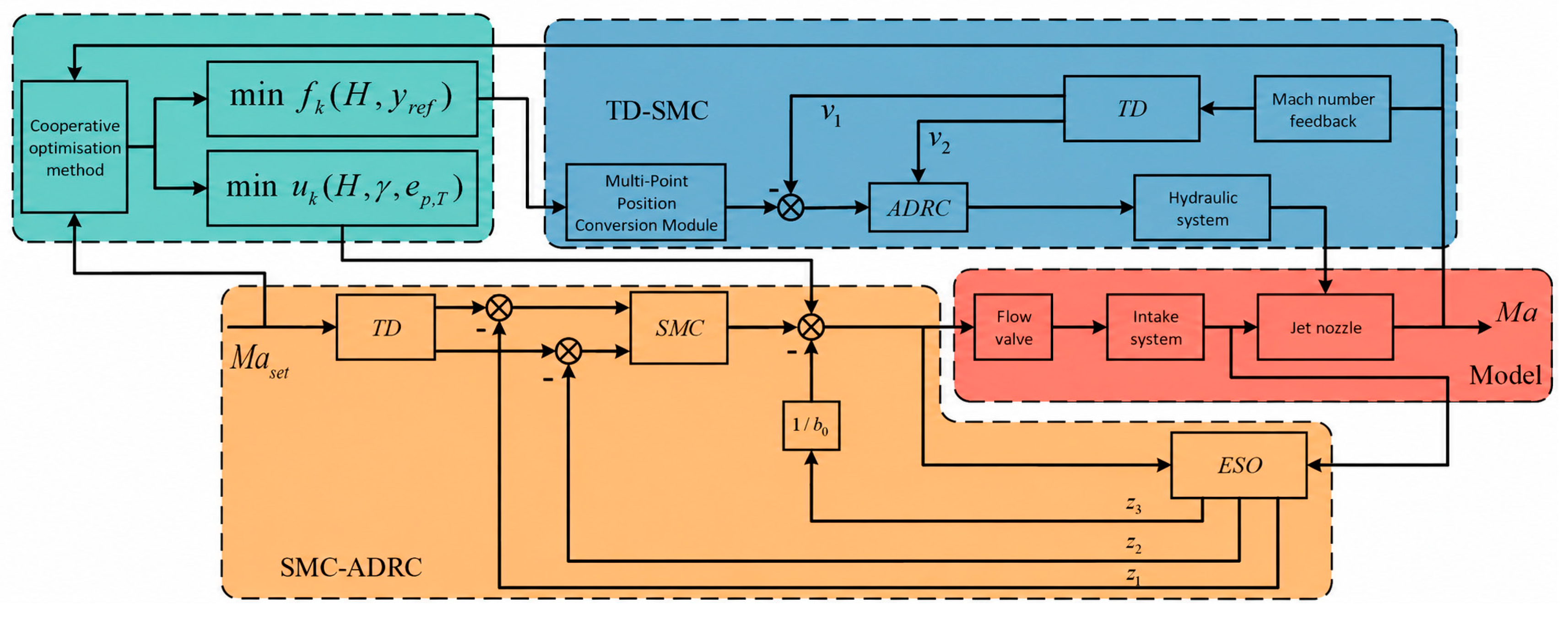
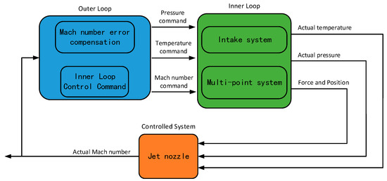
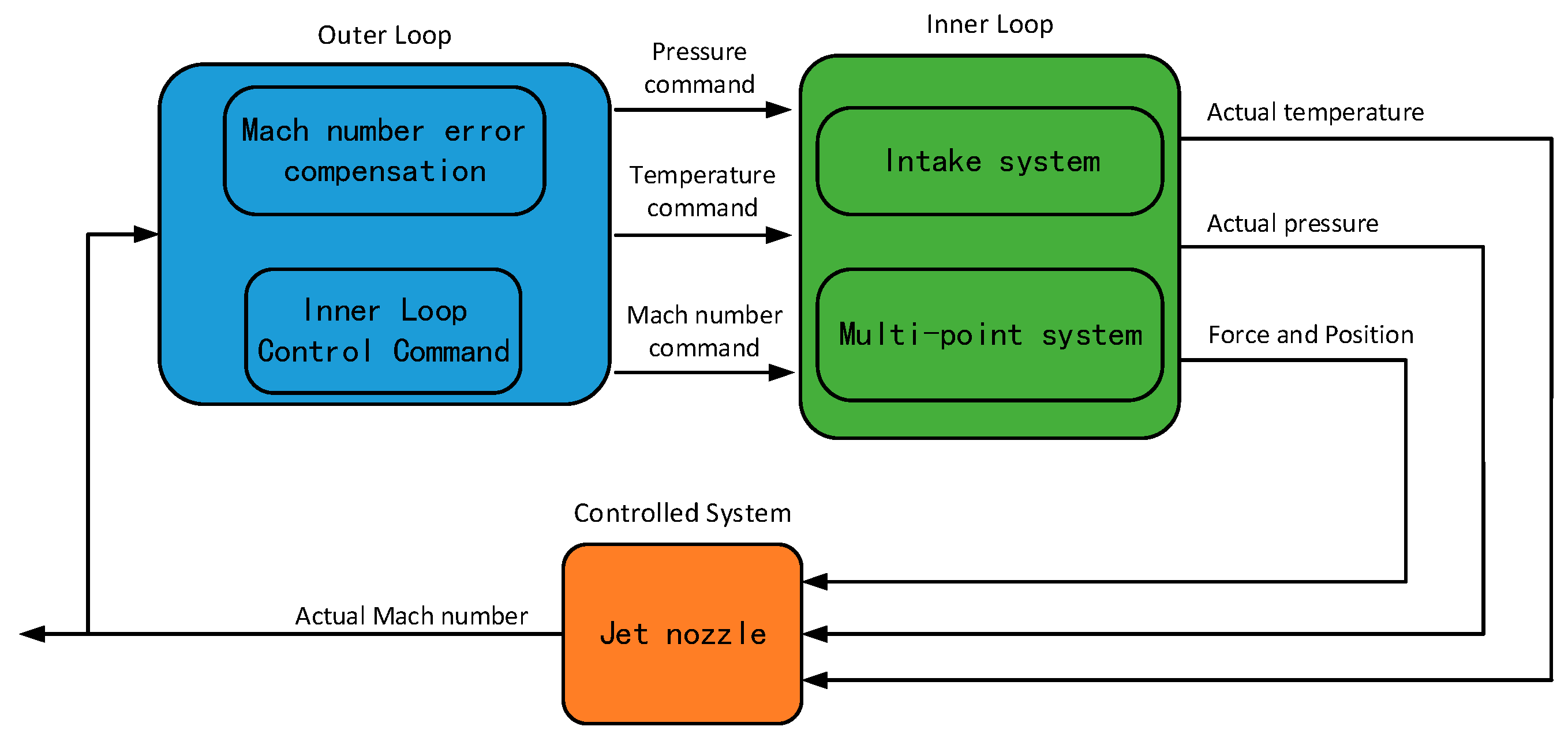
Based on the preceding analysis, the inner loop comprising the intake system and multi-point system can achieve convergence under their respective algorithms and controllers. The inner loop’s output fed to the jet nozzle yields the system’s actual output Mach number. However, as the jet nozzle constitutes a large and complex nonlinear system subject to numerous disturbances and uncertainties, relying solely on the intake system and multi-pivot system for control may result in a certain error between the final actual Mach number and the Mach number command. Employing the intake system and multi-point system as the inner-loop control, while additionally incorporating Mach number error feedback compensation as the outer-loop control, enables this design to address discrepancies between the actual Mach number and the Mach number command. It simultaneously enhances the system’s robustness and stability. The dual-loop design framework is illustrated in Figure 5.

Figure 5. Dual-loop design structure diagram.

Based on the standard atmospheric model and the barometric equation, the following formulae may be derived for the variation in static temperature (K) and pressure (Pa) with height (km):

$$\begin{array}{l}{T}_H=\left\{\begin{array}{l}{T}_0-LH, \mathrm{H}\le \overline{H}\\ T_1, \mathrm{H}>\overline{H}\end{array}\right.\\ P_H=\left\{\begin{array}{l}{P}_0{(1-{\displaystyle \frac{LH}{T_0}})}^{{\displaystyle \frac{g}{RL}}}, \mathrm{H}\le \overline{H}\\ P_1{e}^{-{\displaystyle \frac{g(H-\overline{H})}{R{T}_1}}}, \mathrm{H}>\overline{H}\end{array}\right.\end{array}$$

(74)

where $T_0,P_0$ denote the initial temperature and pressure at sea level; $T_1,P_1$ denote the initial temperature and pressure in the stratosphere; $\overline{H}$ represents the boundary height between the troposphere and stratosphere; $L$ signifies the linear lapse rate; $g$ denotes the gravitational acceleration; $R$ represents the gas constant.

Based on the static total relations for isentropic compressible flow, the relationship between Mach number and temperature–pressure can be expressed as follows:

$$\left\{\begin{array}{l}T=T_H(1+{\displaystyle \frac{k-1}{2}}M{a}^2)\\ P=P_H{(1+{\displaystyle \frac{k-1}{2}}M{a}^2)}^{{\displaystyle \frac{k}{k-1}}}\end{array}\right.$$

(75)

where $Ma$ denotes the Mach number; $k$ represents the specific heat ratio of air.

The outer loop generates a correction term via a PID controller based on the deviation between the actual Mach number and the Mach number command. This correction is fed back as compensation to the inner loop command generation function. Subsequently, ADRC may be employed as required to further compensate for disturbances in the outer loop, thereby enhancing the system’s robustness and stability.

5. Numerical Simulation and Validation

This section primarily employs numerical simulation to verify whether the previously designed control algorithm meets actual control requirements. Based on the simulation results, process comparisons and data analysis are conducted, enabling further conclusions to be drawn based on the quality of the analysis outcomes.

5.1. Simulation Metrics and Process Description

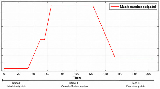
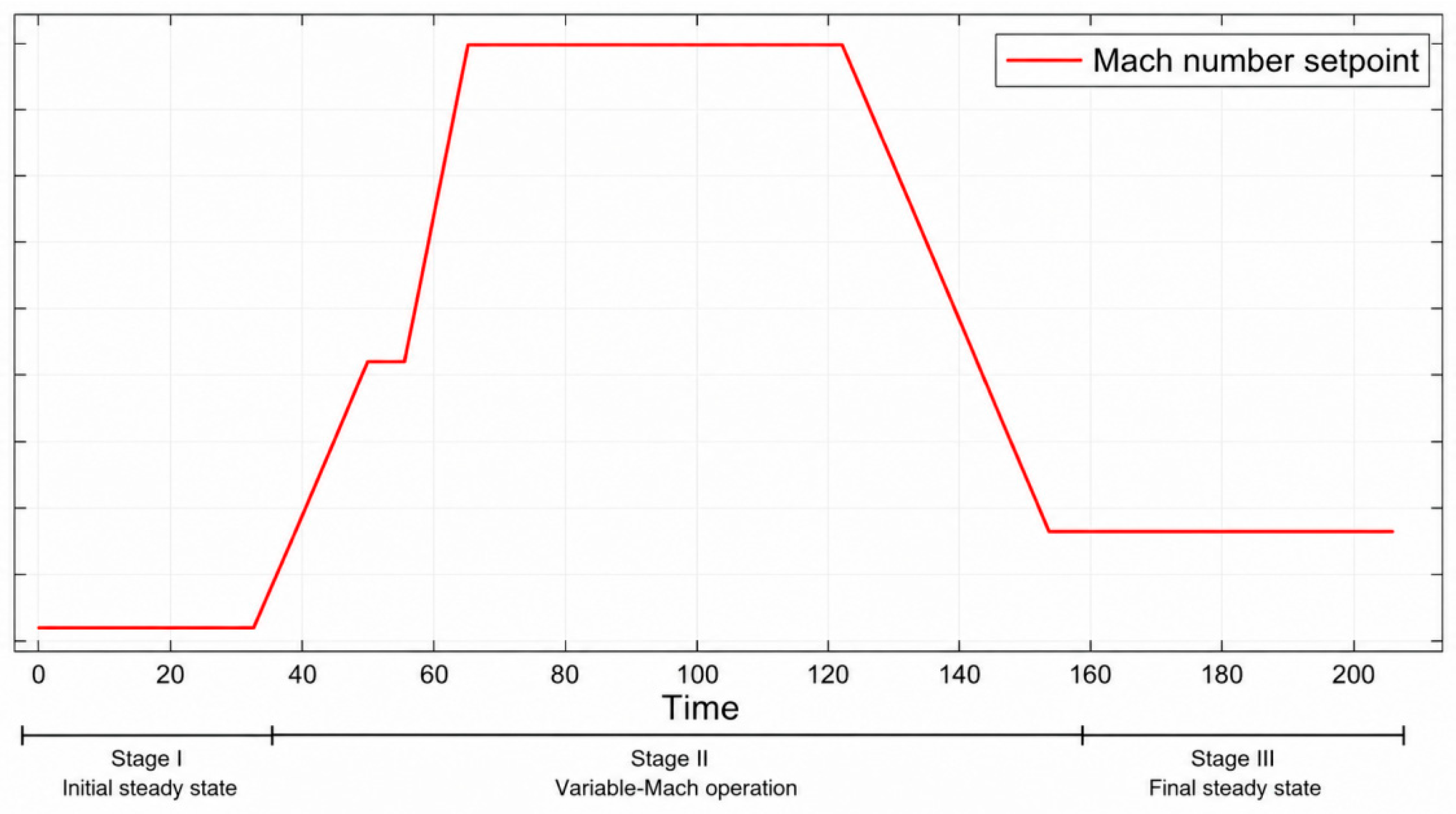
To validate the designed integrated ADRC method based on collaborative optimization, numerical simulation experiments were conducted. The experiments can be divided into three stages according to Mach number variations, with the specific Mach number changes illustrated in Figure 6:

Figure 6. Mach number command diagram.

• Stage One: From 0 to 30 s, the Mach number was set to simulate the critical state of a supersonic nozzle. As the Mach number remained constant, the temperature and pressure required for the nozzle’s operating conditions remained largely unchanged, with the positions of all points remaining fixed.
• Stage Two: From 30 to 152 s, the nozzle underwent continuous variable Mach number operation, rising from a minimum of Mach to a maximum over 35 s and subsequently remaining stable for 57 s. Then, the Mach number decreased from maximum to 1.5 during 30 s. The continuous variable Mach number caused the operating condition of the nozzle to keep varying, which in turn modified the temperature and pressure control targets of the intake system and the position control targets for the individual pivots within the multi-pivot subsystem.
• Stage Three: From 152 s until simulation completion, the Mach number was consistently maintained at a constant value, simulating the stable operating state of the nozzle. At this point, both the air intake subsystem and the multi-pivot system remained in a relatively stable condition. The control parameters for both subsystems remained unchanged, though differing from those of the first stage.

5.2. Comparison and Analysis of Simulation Results

During numerical simulation, the initial thermodynamic state of the intake system is defined as follows: the total temperature of the high-temperature flow path fluid is 900.15 K, with a total pressure set at 180 kPa; the total temperature of the low-temperature flow path fluid is 437.15 K, with a total pressure of 140 kPa. The initial state of the chamber is based on standard atmospheric conditions, with an internal working fluid temperature of 288.15 K and an initial pressure of 101.3 kPa. Cooperative optimization parameters: error term coefficients ${\gamma }_1=5\times {10}^{-5};{\gamma }_2=5\times {10}^{-5}$; energy consumption coefficient matrix $H=[0.7,0.5;0.5,0.7]$; pressure-temperature control variable constraint coefficients $k_{11}=2,k_{12}=0.5,k_{21}=3,k_{22}=0.5$. Key controller parameters are shown in Table 1.

Table 1. Key controller parameters.

Control Method	Observer Parameters	Controller Parameters
PID	$\left\{\begin{array}{l}{\omega }_{Op}=15,\\ {\omega }_{OT}=15,\end{array}\right.$	$\left\{\begin{array}{l}k{p}_p=10,k{d}_p=3,\\ k{p}_T=10,k{d}_T=3,\end{array}\right.$
SMC-LADRC	$\left\{\begin{array}{l}{\omega }_{Op}=15,\\ {\omega }_{OT}=15,\end{array}\right.$	$\left\{\begin{array}{l}{\lambda }_P=10,{\omega }_P=10,k_{s_p}=-10,k_1=-5,\\ {\lambda }_T=2,{\omega }_T=7,k_{s_p}=-1,k_1=-2,\end{array}\right.$
Multi-Point Hydraulic Press System	$\left\{\begin{array}{l}{\beta }_1=60,\\ {\beta }_2=1.2\times {10}^3,\\ {\beta }_1=8\times {10}^3\end{array}\right.$	$\left\{\begin{array}{l}m=1,n=10,k=5,b=5,\\ {\omega }_n=33.6,\zeta =1.17,\\ k_1=1125,k_2=75\end{array}\right.$

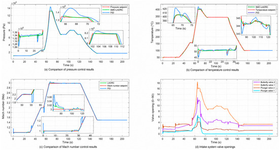
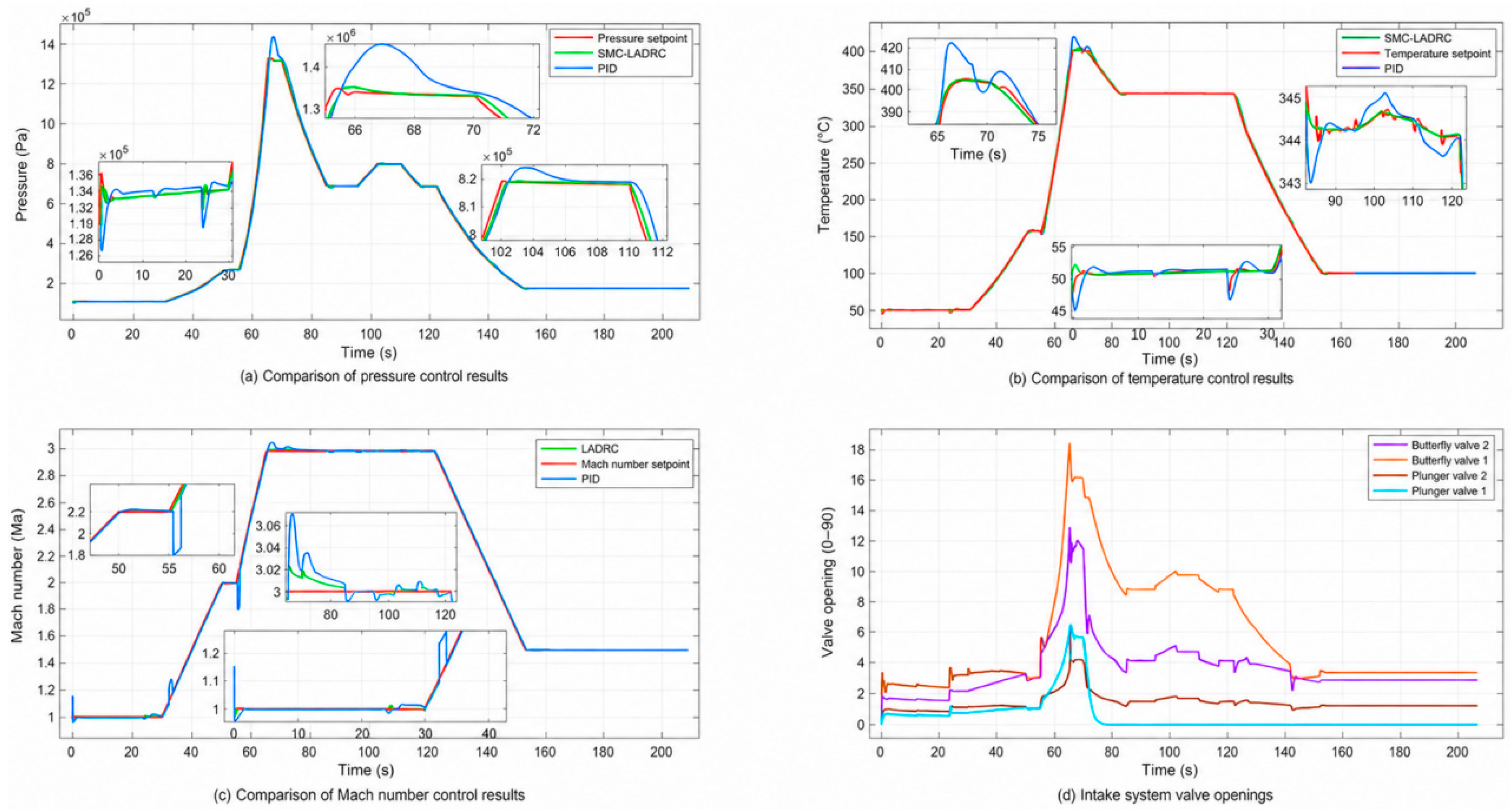
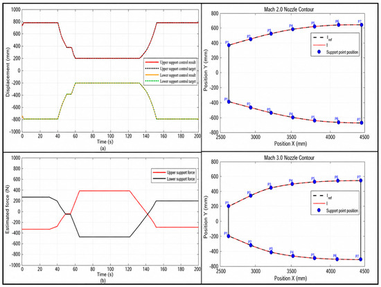
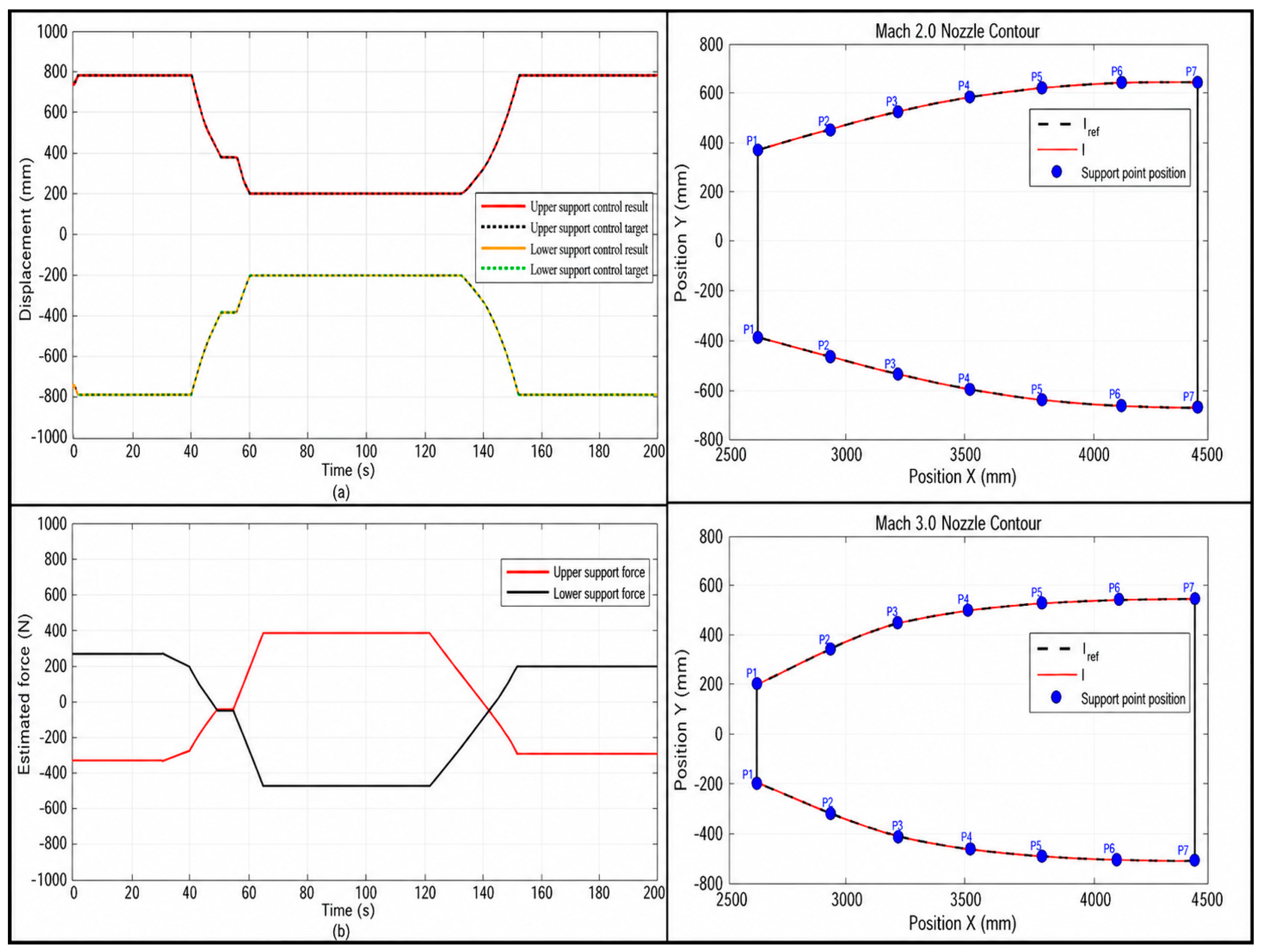
Simulation tests were conducted using the initial condition parameters, cooperative optimization parameters, and main controller and observer parameters derived from the simulation. The simulation results are shown in Figure 7 and Figure 8.

Figure 7. Intake system control results chart.

Figure 8. Throat pivot control and nozzle profile diagram. (a) Nozzle support control result. (b) Nozzle support control force.

The simulation results reveal that, during the first phase, with Mach number remaining constant, both temperature and pressure in the intake system remained relatively stable. However, the PID control exhibited errors of approximately 0.15 Ma at around 0–2 s and 25 s due to disturbances, leading to a maximum deviation of 6.6 kPa in intake pressure and 5 °C in temperature, with a net tracking error of about 0.01 Ma. The SMC-LADRC demonstrated superior disturbance suppression between 0–2 s and 25 s, producing a maximum Mach number error of approximately 0.015 Ma and a net tracking error of about 0.005 Ma. The intake system pressure exhibited a maximum deviation of 3.12 kPa, while the temperature showed a maximum deviation of 2.3°.

During the second phase, as the Mach number climbed from 1 Mach to 2 Mach, the PID control exhibited approximately 1 s of oscillation at simulation time 55 s. This oscillation caused a maximum Mach number deviation of about 0.21 Mach, further leading to control errors of 25 kPa in intake system pressure and 7.3 °C in temperature. In contrast, the SMC-LADRC system showed no significant Mach number oscillation. After simulation time 55 s, the Mach number entered a rapid ascent phase, reaching Mach 3 at approximately 65 s. Simulation results clearly show both control methods exhibit minimal tracking error during Mach number increase, averaging around 0.02 Ma. However, when the Mach number stabilized, the PID control exhibited an overshoot of approximately 0.07 Ma (about 2.3%). Although the Mach number error was smaller than before, its absolute value was significantly higher at this stage, exerting a greater impact on the system. This directly led to a pressure error of 117.32 kPa (approximately 8.8%) and a temperature error of 18.5 °C (approximately 4.6%).

This was accompanied by noticeable pressure and temperature fluctuations, which gradually converged only after 20 s. In contrast, the SMC-LADRC control exhibited a maximum Mach number overshoot of approximately 0.023 Ma (0.76%), leading to a maximum pressure error of 16.5 kPa (1.2%), with a maximum temperature error of 2.67 °C (0.67%). Furthermore, subsequent Mach number fluctuations caused by the outer-loop compensation were smoother than those of the PID system, and convergence was significantly faster.

After approximately 152 s of simulation time in the third phase, the Mach number stabilized at 1.5 Ma. Both control methods achieved final steady-state errors below 0.003 Ma. However, during convergence, the PID control exhibited overshoot of up to 0.06 Ma, resulting in maximum errors of 3.45 kPa in intake system pressure and 1.23 °C in temperature. In contrast, the Mach number curve under SMC-LADRC control converged with virtually no overshoot, resulting in superior control accuracy for both temperature and pressure in the intake system. Figure 7d illustrates the valve openings of the four intake valves under coordinated optimized fault-tolerant control. During the Mach number climb phase from 30 s to 152 s in Stage 2, the intake system experienced highly volatile temperature and pressure fluctuations, and valve opening changes are most significant. However, at 70 s into the simulation, Plunger Valve 1 gradually closes due to an anomaly. Through coordinated control, the opening of Butterfly Valve 1 compensates for the entire intake system, ensuring the system ultimately maintains normal operation in the simulation results.

In actual multi-pivot systems, each pivot point requires control by a hydraulic actuator. To simplify simulation, hydraulic actuator control was applied only to the upper and lower pivot points of the nozzle throat in this study. The default control results for the remaining pivot points were deemed to have achieved the command targets, based on the multi-pivot coordination algorithm and ADRC hydraulic actuator control. Simulation results demonstrate that the throat pivot control consistently achieves excellent tracking of theoretical control targets across all Mach number transition phases. The multi-pivot system ensures nozzle profile compliance during Mach number changes, thereby further guaranteeing stability in the final actual Mach number output. When all other pivots are simulated using the cooperative optimization algorithm and ADRC hydraulic control framework, the nozzle profile dynamically adapts to Mach number variations. Due to the diversity of nozzle profile variations, it is impractical to list all final simulation results. Figure 8 presents the multi-pivot profile control outcomes for Mach 2 and Mach 3 conditions.

6. Conclusions

This paper proposes an integrated ADRC method based on cooperative optimization for free-jet nozzle systems. Through theoretical analysis and numerical simulations, the effectiveness of the designed controller is validated, leading to the following conclusions:

(1)

For multi-pivot control of free-jet nozzles, a cooperative optimization method is introduced. The convergence of the proposed approach is demonstrated, providing essential conditions for subsequent design of a multi-pivot controller.

(2)

A “multi-valve cooperative fault tolerance” mechanism is designed. By integrating the cooperative optimization method with the SMC-LADRC control algorithm, a cooperative fault-tolerant controller is developed. The stability of the mechanism is verified, with improved control accuracy and robustness.

(3)

Simulation verification of the proposed method was conducted. The results demonstrate that the proposed method not only ensures stable operation in the event of an intake system valve anomaly, but also achieves higher control accuracy for pressure, temperature, and Mach number, along with stronger disturbance rejection capability.

The integrated cooperative fault-tolerant ADRC method proposed in this paper adopts a distributed approach by dividing the entire jet nozzle system into two subsystems for control. Future work may consider incorporating a centralized control objective function to achieve improved control performance.

References

- Hou, M.J. High-Altitude Simulation Testing Technology; Aviation Industry Press: Beijing, China, 2014. [Google Scholar]
- Weisser, M.; Bolk, S.; Staudacher, S. Hardware-in-the-Loop-Simulation of a Feedforward Multivariable Controller for the Altitude Test Facility at the University of Stuttgart; Deutsche Gesellschaft für Luft-und Raumfahrt-Lilienthal-Oberth eV: Bonn, Germany, 2013. [Google Scholar]
- Xin, G. A Study on High-Altitude Simulation Testing Technology for Russian Connecting High-Altitude Platforms. Aircr. Engine 1998, 19, 24–28. [Google Scholar]
- Zhan, P.G. Research on the Construction of a 4.9 m-Scale Large Transonic Wind Tunnel. Aerodyn. Missile J. 2014, 40–43. [Google Scholar] [CrossRef]
- Zhang, Z.R. Optimization of the Aerodynamic Layout of a Supersonic-Subsonic High-Altitude Free-Jet Simulation Test Facility. Master’s Thesis, Shenyang Aerospace University, Shenyang, China, 2016. [Google Scholar]
- Yao, Y.L.; Yuan, H.C.; Wu, F.; Leng, L.T. Modeling and simulation study of a free-jet high-altitude simulation test rig system. Meas. Control. Technol. 2021, 40, 89–95. [Google Scholar]
- Xu, X.; Wu, Y.Z.; Cheng, K.M.; Wang, Z.J. Aerodynamic layout design of a hypersonic wind tunnel. J. Nanjing Univ. Aeronaut. Astronaut. 2008, 40, 271–274. [Google Scholar]
- Chen, P.F.; Wu, F.; Wang, J.J. Research progress of free-jet nozzle technology. Aero-Engine 2022, 48, 62–69. [Google Scholar]
- Wu, L.F.; Qian, Q.M.; Zhai, C.; Zhang, H.H.; Xu, Z.Z. Adaptive Active Disturbance Rejection Control Based on Coupling Degree Identification and Its Application in Flight Environment Simulation System. J. Propuls. Technol. 2026, 47, 248–264. [Google Scholar]
- Zhang, H.H.; Dan, Z.H.; Wang, X.; Qian, Q.M.; Li, C.J. Alitude simulation test cell flight enviroment simulation via noise supperesion based active disturbance rejection control. Gas Turbine Exp. Res. 2026, 39, 29–40. [Google Scholar] [CrossRef] [Scilit]
- Zhang, L.Y.; Shi, D.Q.; Zhai, C.; Dan, Z.H.; Zhang, H.H.; Wang, X.; Xiao, G.X. Coordinated Multi-Valve Disturbance-Rejection Pressure Control for High-Altitude Test Stands via Exterior Penalty Functions. arXiv 2025, arXiv:2505.09352. [Google Scholar] [CrossRef] [Scilit]
- Yu, C.G.; Zhang, Z.L.; Lai, H.; Chen, W.H.; Chen, Z.H.; Nie, X.T. Semi-analytic solution and verification for large deflection forming of single-jack semi-flexible nozzle based on elliptic integral. J. Aerosp. Power 2022, 37, 383–390. [Google Scholar]
- Zheng, L.X.; Wang, W.B.; Zhang, Y.Y.; Wang, L.M.; Lu, W. Optimization Analysis of the Mixing Chamber and Diffuser of Ejector Based on Fano Flow Model. Comput. Model. Eng. Sci. 2022, 133, 153–170. [Google Scholar] [CrossRef] [Scilit]
- Wang, C.C.; Hu, C.Y.; Li, W.; Xu, H.L.; Miao, K.Q.; Sun, J.X. Mixer Temperature Prediction via Decomposed Transformer and xLSTM with Physical Constraints. Symmetry 2025, 17, 1441. [Google Scholar] [CrossRef] [Scilit]
- Zhang, L.Y.; Zhang, H.H.; Shi, D.Q.; Dan, Z.H.; Wang, X.; Zhai, C.; Xiao, G.X.; Xu, Z.Z. Fixed-Time Active Disturbance Rejection Temperature–Pressure Decoupling Control for a High-Flow Air Intake System. Entropy 2025, 27, 880. [Google Scholar] [CrossRef] [Scilit]
- Qi, X.; Fang, Y.F.; Li, X.; Zhai, C.; Zhang, H.H.; Zhao, W. Decentralized Optimization Approach for Modeling and Cooperative Control of Pressure Regulation System in Environmental Simulation Facility. Modelling 2026, 7, 59. [Google Scholar] [CrossRef] [Scilit]
- Parikh, N.; Boyd, S. Proximal Algorithms. Found. Trends Optim. 2014, 1, 127–239. [Google Scholar] [CrossRef] [Scilit]
- Boyd, S.; Vandenberghe, L. Convex Optimization; Cambridge University Press: Cambridge, UK, 2004. [Google Scholar]
- Nesterov, Y. Introductory Lectures on Convex Optimization: A Basic Course; Springer Science & Business Media: Berlin, Germany, 2013. [Google Scholar]
- Sontag, E.D. Smooth stabilization implies coprime factorization. IEEE Trans. Autom. Control. 1989, 34, 435–443. [Google Scholar] [CrossRef] [Scilit]
- Young, W.H. On Classes of Summable Functions and Their Fourier Series. Proc. R. Soc. London. Ser. A Contain. Pap. A Math. Phys. Character 1912, 87, 225–229. [Google Scholar] [CrossRef] [Scilit]
- Sontag, E.D. Input to State Stability: Basic Concepts and Results. In Nonlinear and Optimal Control Theory; Lecture Notes in Mathematics; Nistri, P., Stefani, G., Eds.; Springer: Berlin/Heidelberg, Germany, 2008; Volume 1932, pp. 163–220. [Google Scholar] [CrossRef] [Scilit]
Disclaimer/Publisher’s Note: The statements, opinions and data contained in all publications are solely those of the individual author(s) and contributor(s) and not of MDPI and/or the editor(s). MDPI and/or the editor(s) disclaim responsibility for any injury to people or property resulting from any ideas, methods, instructions or products referred to in the content. |
© 2026 by the authors. Licensee MDPI, Basel, Switzerland. This article is an open access article distributed under the terms and conditions of the Creative Commons Attribution (CC BY) license.