Correcting SLD Icing Parameters: A Ridge Regression Method Fusing Icing Wind Tunnel Data and Numerical Priors

Abstract

To explore the significant systematic deviations of FENSAP-ICE numerical simulations under supercooled large droplet (SLD) conditions, a ridge regression correction method that integrates numerical priors and domain-knowledge-aided features for ice shape geometric parameters is presented in this manuscript. The FENSAP-ICE predictions of eight geometric ice shape parameters are incorporated as numerical priors into the machine learning model, transforming the learning objective from “predicting from scratch” to “correcting systematic bias.” Six engineering auxiliary features are constructed based on SLD icing physics to provide physically meaningful adjustable dimensions for small-sample modeling. A two-stage model combining Logistic Regression classification and Ridge Regression is designed for zero-ice cases on the lower-surface icing limit. Evaluated via Leave-One-Out Cross-Validation on 29 sets of NACA0012 airfoil SLD icing wind tunnel experimental data, the improved system reduces the sMAPE of total ice area from 79.47% to 34.65%, lower-surface ice horn angle from 105.19% to 28.08%, upper-surface icing limit from 61.75% to 35.48%, and average ice thickness from 42.12% to 20.89%, all compared with FENSAP-ICE predictions. Ablation experiments further reveal that the introduction of the numerical prior alone reduces prediction error by approximately 10 percentage points, serving as the primary performance driver. The proposed method features low computational cost and strong physical consistency, providing a practical bias-correction framework for SLD ice shape prediction under small-sample conditions. Furthermore, to address the potential optimistic bias arising from small-sample cross-validation, nested cross-validation together with multiple linear baseline models are additionally employed to verify the robustness and relative competitiveness of the proposed correction method.

1. Introduction

Aircraft icing remains a constant hazard for aviation safety. Ice accretions alter the aerodynamic shape of wings, inducing lift loss and drag increase, and can precipitate loss-of-control accidents under severe conditions [1]. The problem becomes particularly complex and hazardous in the presence of supercooled large droplets (SLDs), defined as supercooled droplets with a median volumetric diameter (MVD) exceeding 50 μm. Such droplets undergo significant deformation, breakup, and splashing prior to impingement on the airframe [2,3]. Broeren et al. demonstrated in their swept-wing SLD ice accretion study that once ice propagates beyond the protected region of an ice protection system, lift losses exceeding 30% can occur within minutes, underscoring the urgency of accurate SLD ice shape prediction [4].

In engineering practice, numerical icing codes such as FENSAP-ICE, although the mainstream tool for ice protection design, systematically underestimate the SLD ice shape, and in particular the upper- and lower-surface icing limits; adopting such results directly leads to undersized ice protection regions and severe residual icing aft of the protected area. Existing physics-informed machine learning approaches alleviate the scarcity of experimental data mainly by embedding governing-equation constraints or by performing domain transfer, but they have not been systematically applied to correcting the bias of SLD icing simulations. To fill this gap, the present study treats the FENSAP-ICE prediction as a numerical prior and employs ridge regression to learn its systematic deviation from icing wind tunnel measurements, thereby correcting the key ice shape parameters at low computational cost.

Numerical simulation tools, typified by FENSAP-ICE, constitute the mainstream approach for icing prediction. FENSAP-ICE solves the droplet momentum equations via an Eulerian-Eulerian formulation and couples the Messinger thermodynamic model through its ICE3D module to compute three-dimensional ice shapes [5]; it has been extensively validated under conventional icing conditions [6]. Under SLD conditions, however, the rigid-sphere assumption and the full-capture assumption inherent in conventional models no longer hold [3,7], leading to pronounced systematic deviations. Hu et al. confirmed that FENSAP-ICE fails to accurately capture ice horns under glaze and mixed icing regimes, producing substantial errors in both ice thickness and icing extent [8].

In recent years, machine learning methods have been widely introduced into the icing prediction field. On the traditional machine learning front, Chang et al. combined wavelet packet transforms with artificial neural networks to predict ice accretion on airfoil surfaces [9]; Li et al. employed an XGBoost algorithm to rapidly assess icing severity using liquid water content, droplet diameter, and exposure time as inputs [10]. Pan et al. employed a Random Forest model to establish the mapping from common meteorological parameters to in-cloud microphysical parameters (MVD and LWC), which then serve as inputs for ice accretion simulation on a specific airfoil [11]. In the realm of deep learning, Strijhak et al. trained neural networks on iceFoam simulation data for ice shape prediction [12]; Dong applied a combined CNN-RNN architecture for in-flight icing identification [13]. He Lei et al. employed a transposed convolutional neural network, trained on a NACA0012 airfoil numerical ice shape dataset, to achieve image-based ice shape prediction [14]. More recently, Xu et al. developed a PyTorch-based deep neural network (DNN) for efficient airfoil rime icing prediction, using OpenFOAM-initialized flow fields as inputs to establish a nonlinear mapping to droplet field variables, achieving traditional numerical accuracy with negligible computational cost [15]. While these methods achieve satisfactory accuracy on their training distributions, they collectively confront a bottleneck, in that icing wind tunnel experimental data are extremely scarce, as an entire SLD test matrix typically yields only a few dozen valid samples, and complex network models are highly susceptible to overfitting under such small-sample regimes [16,17].

Beyond ice shape prediction, machine learning has also been actively applied to the performance modeling of aircraft anti-icing systems and ground de-icing fluids. Abdelghany et al. combined artificial neural networks (ANNs) with the Internet of Things (IoT) to predict wing anti-icing system temperatures based on experimental and CFD data, demonstrating that the ANN approach significantly outperforms traditional CFD simulations in both accuracy and computational efficiency [18]. Cardona et al. systematically evaluated Decision Tree, Random Forest, and XGBoost models for predicting anti-icing fluid endurance time under natural and artificial snow conditions, finding that the optimized XGBoost model effectively captures the nonlinear interactions between snowfall rate and ambient temperature, providing data-driven support for winter ground operation safety [19]. In the analogous field of wind turbine icing, Kallarappayi et al. benchmarked multiple ML and DL models across different forecast horizons, concluding that ensemble learning methods like Random Forest offer the best balance between accuracy and execution speed, and that input data richness is more critical than model complexity [20].

The emergence of Physics-Informed Machine Learning (PIML) offers a new paradigm to alleviate the small-sample predicament. Raissi et al. proposed Physics-Informed Neural Networks (PINNs), embedding partial differential equations as loss terms during training [21]; Ling et al. embedded tensor invariances into deep neural networks, considerably improving the generalization capability of turbulence models [22]; Carleo et al. systematically reviewed machine learning applications in the physical sciences, identifying the deep integration of physical knowledge with data-driven approaches as a crucial direction for solving complex scientific problems [16]. In icing-related domains, Wang Zhenguo et al. fused PINNs with self-transfer learning to propose a physics-knowledge-guided iterative self-transfer model for ice accretion prediction on power lines, achieving notable improvements [23].

The aforementioned work demonstrates that infusing physical knowledge can effectively compress the demand for training data. However, existing PIML methods predominantly focus on embedding partial differential equation constraints or performing domain transfer, and have yet to be systematically applied to the problem of bias correction in SLD icing numerical simulations. A promising yet underexplored paradigm is bias correction, in which, rather than discarding the existing physical model, one employs machine learning to learn the systematic deviation between numerical simulation outputs and experimental measurements, thereby retaining the flow field, droplet impingement, and thermodynamic information encapsulated in the physical model as a prior and substantially reducing the modeling difficulty [22,24].

Addressing this gap, the present paper proposes an improved SLD ice shape prediction method that integrates FENSAP-ICE numerical priors with domain-knowledge-aided features. The eight ice shape geometric parameter predictions output by FENSAP-ICE are introduced into the machine learning model as numerical priors, transforming the learning objective from “predicting from scratch” to “correcting systematic bias.” Six engineering auxiliary features, constructed based on the physical mechanisms of SLD icing, provide the small-sample model with physically meaningful, adjustable degrees of freedom. Ridge regression serves as the core algorithm, with L2 regularization employed to suppress overfitting under small-sample conditions. The entire framework is evaluated via leave-one-out cross-validation on 29 sets of NACA0012 airfoil SLD icing wind tunnel experimental data, ultimately yielding an ice shape prediction correction model characterized by low computational cost and strong physical consistency. To rigorously assess the generalization capability under the small-sample constraint, the correction results are further validated through nested cross-validation and cross-checked against several linear baseline models.

2. Data and Feature Engineering

2.1. Experimental Conditions and Ice Shapes

To systematically investigate ice shape characteristics under SLD conditions, icing experiments were conducted at the FL-16 icing wind tunnel of the China Aerodynamics Research and Development Center on a NACA0012 airfoil with a 1 m chord length. A total of 29 test conditions were designed, with the angle of attack ranging from 0° to 4.9°, static temperature from 253.15 K to 268.55 K, liquid water content (LWC) from 0.21 g/m³ to 0.50 g/m³, MVD from 19 μm to 526 μm, and icing time from 120 s to 1350 s. These condition parameters are summarized in Table 1.

Table 1. Experimental condition parameters.

NO	v (m/s)	AOA (°)	Pressure (Pa)	Icing Time (s)	Temperature (K)	MVD (μm)	LWC (g/m3)
01	95	4.9	59,524	660	266.55	20	0.50
02	95	4.9	59,524	1320	268.55	20	0.50
03	95	0.0	59,524	660	266.55	20	0.50
04	95	4.9	59,524	120	266.55	20	0.50
05	61	0.0	101,325	300	253.15	20	0.21
06	95	4.9	59,524	660	266.55	20	0.40
07	95	4.9	59,524	660	268.55	20	0.40
08	95	4.9	59,524	1350	268.55	20	0.40
09	95	0.0	59,524	660	266.55	20	0.40
10	95	4.9	59,524	120	266.55	20	0.40
11	61	0.0	101,325	300	253.15	20	0.40
12	95	4.9	59,524	660	266.55	110	0.25
13	95	4.9	59,524	660	268.55	110	0.25
14	95	4.9	59,524	1350	268.55	110	0.25
15	95	0.0	59,524	660	266.55	110	0.25
16	95	4.9	59,524	120	266.55	110	0.25
17	61	0.0	101,325	300	253.15	110	0.25
18	95	4.9	81,506	660	266.55	19	0.28
19	95	4.9	81,506	660	268.55	19	0.28
20	95	4.9	81,506	1350.6	268.55	19	0.28
21	95	0.0	81,506	660	266.55	19	0.28
22	95	4.9	81,506	120	266.55	19	0.28
23	61	0.0	101,325	300	260.15	19	0.28
24	95	4.9	81,506	660	266.55	526	0.24
25	95	4.9	81,506	660	268.55	526	0.24
26	95	4.9	81,506	1350	268.55	526	0.24
27	95	0.0	81,506	660	266.55	526	0.24
28	95	4.9	81,506	120	266.55	526	0.24
29	61	0.0	101,325	300	260.15	526	0.21

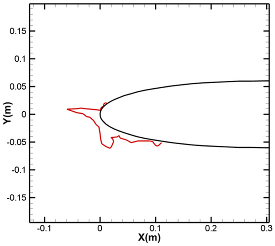
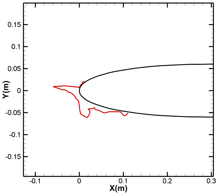
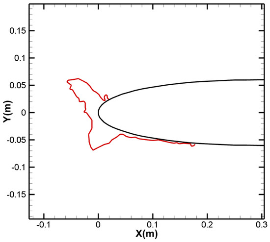
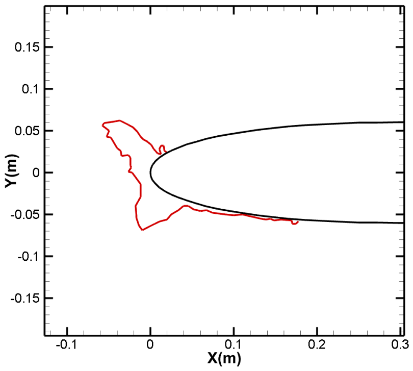
The discrete coordinates of the ice shapes accreted on the airfoil surface were recorded during the experiments. Owing to the large number of test conditions, Figure 1 and Figure 2 present the experimental ice shapes for Conditions 1 and 2 from Table 1, respectively.

Figure 1. Experimental ice shape for NO. 01.

Figure 2. Experimental ice shape for NO. 02.

2.2. FENSAP-ICE Simulation and Ice Shapes

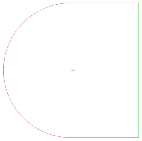
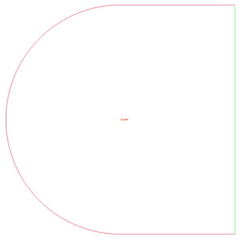
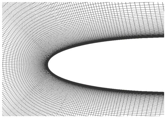
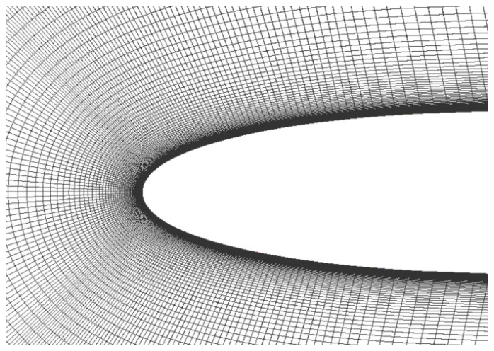
Since icing wind tunnel experiments are costly and cannot achieve a sufficiently dense distribution of test parameters, this study employs a commercial icing code to simulate SLD ice shapes and subsequently performs physically guided bias correction of the numerical results based on experimental data. A geometric model identical to the experimental NACA0012 airfoil was constructed, as shown in Figure 3, and the structured mesh depicted in Figure 4 was generated; mesh independence was verified.

Figure 3. NACA0012 flow field geometric model.

Figure 4. Close-up view of the structured mesh on the NACA0012 surface.

The DROP3D module of FENSAP-ICE solves the droplet impingement process using the Eulerian method. For non-SLD conditions, the governing equations for droplet impingement are:

$${\displaystyle \frac{\partial \mathsf{\alpha }}{\partial \mathrm{t}}} +\overrightarrow{ \nabla }\cdot (\mathsf{\alpha } {\overrightarrow{\mathrm{V}}}_{\mathrm{d}}) = 0$$

(1)

$${\displaystyle \frac{\partial \left(\mathsf{\alpha }{\overrightarrow{\mathit{V}}}_{\mathit{d}}\right)}{\partial \mathit{t}}}+\overrightarrow{ \mathit{V}}\left[\mathsf{\alpha }{\overrightarrow{\mathit{V}}}_{\mathit{d}}\otimes {\overrightarrow{\mathit{V}}}_{\mathit{d}}\right]={\displaystyle \frac{{\mathit{C}}_{\mathit{D}}{\mathit{Re}}_{\mathit{d}}}{24\mathit{K}}}\mathsf{\alpha }\left({\overrightarrow{\mathit{V}}}_{\mathit{s}}-{\overrightarrow{\mathit{V}}}_{\mathit{d}}\right)+\mathsf{\alpha }\left(1-{\displaystyle \frac{{\mathsf{\rho }}_{\mathit{d}}}{{\mathit{\rho }}_{\mathit{d}}}}\right){\displaystyle \frac{1}{{\mathit{Fr}}^2}}$$

(2)

$${\mathit{C}}_{\mathit{D}}={\displaystyle \frac{24}{{\mathit{Re}}_{\mathit{d}}}}(1+0.15{\mathit{Re}}_{\mathit{d}}^{0.687}{)\times (\mathit{Re}}_{\mathit{d}} < 1300)$$

(3)

when Re_d > 1300 and C_D = 0.4.

$${\mathit{We}}_{\mathit{c}}=12\left(1+{1.0770\mathrm{h}}^{1.6}\right)$$

(4)

The PilchErdman model implemented in FENSAP-ICE describes the influence of the breakup phenomenon during SLD impingement based on the Weber number: (4). The Ohnesorge number is defined as:

$$\mathrm{Oh} ={\displaystyle \frac{{\mathsf{\mu }}_{\mathit{d}}}{\sqrt{{\mathsf{\rho }}_{\mathit{d}}{\mathit{d}\mathsf{\sigma }}_{\mathit{d}}}}}$$

(5)

where μ_d is the droplet viscosity, d is the droplet diameter, and σ_d is the droplet surface tension. For water, Oh is on the order of 0.0001; hence, the critical Weber number We_c is approximately 12, where the variables α and V_d are mean field values of the particle concentration and velocity. The first term on the right-hand side of the momentum equation represents the drag acting on particles of mean diameter d. It is proportional to the relative particle velocity, the drag coefficient C_D, and the droplet Reynolds number Re_d. When Re_d > 1300, C_D = 0.4.

The local diameter during the breakup process is solved using:

$${\displaystyle \frac{\mathit{Dd}}{\mathit{Dt}}} = -{\displaystyle \frac{\mathit{d}-{\mathit{D}}_{\mathit{s}}}{\mathsf{\tau }}}$$

(6)

The estimation of the maximum stable diameter is based on the assumption that breakup ceases when the droplet Weber number falls below the critical value of 12:

$${\displaystyle \frac{{\mathit{D}}_{\mathit{s}}}{{\mathit{d}}_0}} = 6.2{\left({\displaystyle \frac{{\mathsf{\rho }}_{\mathit{w}}}{{\stackrel{-}{\mathit{P}}}_{\mathit{a}}}}\right)}^{1/4} {\mathit{Re}}_{{\mathit{d}}^{-1/2}}$$

(7)

When the Weber number is below 12, the drag on the droplet is interpolated between that of a spherical droplet and that of a disk-shaped droplet:

$${\mathit{C}}_{\mathit{D}}{ = \mathit{fC}}_{\mathit{D},\mathit{sphere}} + (1-{\mathit{f})\mathit{C}}_{\mathit{D},\mathit{disk}}$$

(8)

The factor f in the above equation is calculated via:

$$\mathit{f} = 1-{\mathit{E}}^2$$

(9)

where E is determined using the experimental correlation of Hsiang & Faeth:

$$\mathit{E} = {\left(1 + 0.07\sqrt{\mathit{We}}\right)}^{-3}$$

(10)

Two types of splashing and rebound models are available. One, termed the post-processing model, modifies the collection efficiency output by DROP3D by either completely removing the water mass upon rebound or retaining a portion of the impinging water to generate splashing; this method does not permit re-injection of splashed water mass into the computational domain. The other, termed the body-force model, introduces an additional body force near solid surfaces to simulate the influence of wall-droplet interactions on the mean droplet flow. For the range of test conditions investigated in this study, the results obtained by the post-processing model and the body-force model exhibit very small discrepancies, essentially negligible; the body-force model was adopted for the computations in this work.

2.3. Ice Shape Comparison and Geometric Parameter Definition

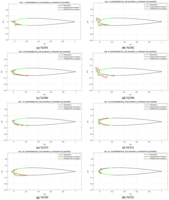
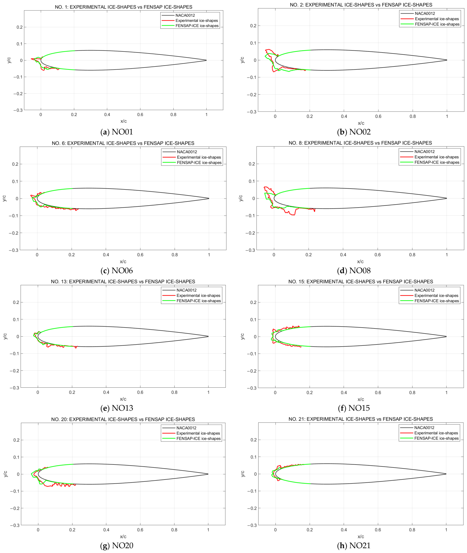
As can be observed from the comparison in Figure 5, the numerical simulation results capture the overall ice shape of SLD icing to a certain extent. However, appreciable deviations from the experimental values are evident in the predicted upper- and lower-surface icing limits and ice horn positions. Notably, for the icing limits, which are parameters of paramount importance for anti-icing and de-icing design, the simulated values for all four conditions shown in Figure 5 are smaller than the experimental measurements. In particular, for Condition NO06, the computed upper- and lower-surface icing limits are less than half of the experimental values. Employing such simulation results for wing thermal ice protection system design would lead to an undersized protection region, causing severe ice accretion aft of the protected area. Consequently, this study proposes constructing a machine learning model to correct the numerical simulation results using experimental ice shapes as the reference, thereby yielding more accurate key ice shape parameters.

Figure 5. Comparison of experimental and numerical ice shapes for different test conditions NO01, 02, 06, 08, 13, 15, 20 and 21.

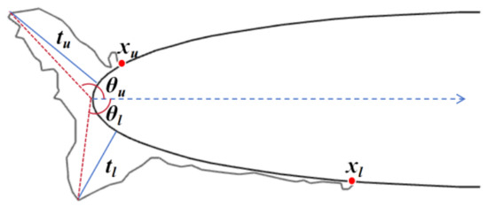
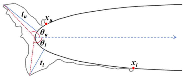
With reference to the SAE AIR5666 standard [25], eight geometric parameters are selected to describe the ice shape on the leading edge of the airfoil, as illustrated in Figure 6.

Figure 6. Schematic of geometric parameters.

In Figure 6, t_u is the upper-surface maximum thickness, mm; t_l is the lower-surface maximum thickness, mm; θ_u is the upper-surface ice horn angle, °; θ_l is the lower-surface ice horn angle, °; x_u is the upper-surface icing limit, mm; x_l is the lower-surface icing limit, mm; and A_total is the total ice area, mm². In addition, the average ice thickness t_avg is defined as a global ice shape feature that reflects the overall icing severity, mm.

Table 2 lists the symmetric mean absolute percentage error (sMAPE) of the FENSAP predictions for the above parameters across the conditions given in Table 1. Because sMAPE normalizes each error by the mean magnitude of the predicted and measured values, it grows disproportionately when the true value is very small. All eight experimental targets here are strictly positive, the smallest being the total ice area of case NO29, about 4 × 10⁻⁵ mm², so the denominator never vanishes. The elevated sMAPE of small-magnitude quantities such as A_total is therefore partly an artefact of this normalisation and should be read with that caveat.

Table 2. sMAPE values of FENSAP predictions for each parameter.

Parameters	sMAPE Values
tu	31.86%
tl	27.96%
Atotal	79.47%
xu	61.75%
xl	59.00%
θu	18.89%
θl	105.19%
tavg	42.12%

2.4. Feature Construction

To establish a mapping from input conditions to output geometric parameters and to provide effective inputs for the subsequent regression models, three distinct categories of feature sets were constructed for different target variables, namely original condition parameters, FENSAP-ICE predictions, and physically motivated auxiliary features. Considering that the experimental velocities in this study are limited to values of 61 m/s and 95 m/s and that excessive features in a small-sample dataset of 29 experiments would induce overfitting, velocity and altitude were not adopted as independent features. Instead, five condition parameters were selected as the primary icing condition features, namely angle of attack (AOA, °), liquid water content (LWC, g/m³), static temperature (T, K), median volumetric diameter (MVD, μm), and icing time (t, s).

Concurrently, the raw predicted values of the eight geometric parameters from FENSAP-ICE were incorporated as part of the model input features, denoted respectively as t_{u_FEN}, t_{l_FEN}, A_{total_FEN}, x_{u_FEN}, x_{l_FEN}, θ_{u_FEN}, θ_{l_FEN}, and t_{avg_FEN}, enabling the machine learning model to learn and correct the systematic bias. These FENSAP-ICE values are used as numerical priors, and the model learns a bias-correction mapping from these priors, together with the condition and engineering features, to the experimental targets. This mapping is evaluated under leave-one-out cross-validation, in which each held-out case is predicted from its own FENSAP prior and the condition features alone, so that the correction is assessed on genuinely unseen cases.

To enhance the generalization capability and physical consistency of the model under small-sample conditions, six engineering features were constructed based on the physical mechanisms of SLD icing. Their specific formulas and physical meanings are detailed in Table 3, and they serve to characterize the key influencing factors in the SLD icing process.

Table 3. Definitions of engineering features.

Feature Name	Formula	Physical Meaning	Construction Basis
Water Collection	LWC · t	Total water droplet collection per unit wingspan length	Cumulative collection directly reflects icing intensity
Temperature Factor	1 − (T − 263.15)/20	Characterizes the influence of temperature on icing type	The temperature of 263.15 K is adopted as a physically motivated reference temperature near the glaze-to-rime icing transition; linear scaling non-dimensionalizes temperature to reflect its effect on the icing type.
MVD Factor	min(MVD/200, 2)	Influence of SLD MVD on icing, normalized to a 200 μm reference	When MVD exceeds 200 μm, SLD-specific breakup and splashing effects become pronounced, and further MVD increases yield diminishing influence; a truncation value of 2 is adopted to prevent leverage effects from a few extremely large MVD conditions
AOA Bias	AOA/5	Influence of angle of attack on icing asymmetry, normalized to a 5° reference	An AOA of 5° covers the experimental AOA range of this study; the scaled magnitude is comparable to other features
Asymmetry	(tu_FEN − tl_FEN)/(tu_FEN + tl_FEN + ε)	Quantifies the degree of icing asymmetry based on the relative difference between FENSAP-predicted upper- and lower-surface thicknesses	FENSAP predictions are used as priors to avoid data leakage that would result from directly using experimental labels; a small constant is added to the denominator to prevent division by zero
Ice volume estimate	Atotal_FEN · tavg_FEN	Estimates the total ice volume based on FENSAP-predicted area and average thickness	The average thickness and total ice area serve as proxies for global icing intensity to reflect overall icing severity

Note: ε = 10⁻⁶ is a small constant to prevent division by zero.

The six engineering features in Table 3 are dimensionless indicators derived from the primary condition parameters. Each is associated with a main physical mechanism of SLD icing, including droplet inertia and impingement, the thermodynamic freezing regime, droplet breakup tendency, and the asymmetry between the upper and lower surfaces. Working with dimensionless features avoids scale mismatch between parameters of different units and is better suited to regression on a small sample.

Furthermore, to obtain a global measure of icing intensity, the average ice thickness tavg is introduced as a key target variable. For the i-th test condition, the average thickness is computed as:

$${\mathit{t}}_{\mathit{avg},\mathit{i}} ={\displaystyle \frac{1}{ {\mathit{N}}_{\mathit{i}}}}{\displaystyle {\displaystyle \sum }_{\mathit{j}=1}^{{\mathit{N}}_{\mathit{i}}}}{\mathit{d}}_{\mathit{i},\mathit{j}}$$

(11)

where Ni is the number of discrete coordinate points of the experimental ice shape for that condition, and d{i,j} is the ice thickness along the normal direction at the j-th coordinate point on the airfoil surface.

2.5. Data Preprocessing

To eliminate differences in dimension and order of magnitude among features and to prevent features with larger magnitudes from dominating model training, Z-score normalization was applied to all continuous input features and target variables. This method transforms the original data to a distribution with a mean of zero and a standard deviation of unity.

For the j-th feature x_j, the normalized value x_j′ is computed via:

$${\mathit{x}}_{\mathit{j}}^{\prime }={\displaystyle \frac{ {\mathit{x}}_{\mathit{j}}-{\mathsf{\mu }}_{\mathit{j}}}{{\mathsf{\sigma }}_{\mathit{j}}}}$$

(12)

Here, μ_j and σ_j are, respectively, the mean and standard deviation of that feature computed on the training set. The normalization parameters are derived exclusively from the training set and subsequently applied to the corresponding test set to prevent data leakage. In the ridge regression implementation, normalization is automatically performed via the ‘Standardize’, true option of the ridge function.

Given the small sample size of 29 cases, a conventional train/validation/test split would substantially reduce the number of training samples, potentially leading to model underfitting. Hence, Leave-One-Out Cross-Validation (LOOCV) was adopted to evaluate model performance. For a dataset comprising n = 29 samples, the procedure iterates n times; in each iteration, a single sample is held out as the test set while the remaining n − 1 samples are used for training. Ultimately, n predictions are obtained and compared with the true values to compute performance metrics. This validation strategy makes maximal use of the limited experimental data for training and evaluation, avoids result fluctuations arising from random partitioning, and ensures the determinism and repeatability of the assessment.

2.6. Modeling Approach

To build a rapid prediction model for the geometric parameters of SLD ice accretion and to achieve effective correction of the systematic bias inherent in FENSAP-ICE numerical simulations, Ridge Regression was selected as the core modeling method. Concurrently, differentiated modeling strategies were designed according to the distinct physical characteristics of each parameter.

Given the small experimental sample size, complex models such as neural networks and deep neural networks are prone to overfitting and find it difficult to effectively learn nonlinear input–output mapping under small-sample conditions. Therefore, ridge regression, an enhanced form of linear regression, was adopted. By introducing an L2 regularization term, it effectively controls model complexity and mitigates overfitting risk. Additionally, ridge regression handles the multicollinearity issues among the original condition parameters, FENSAP predictions, and engineering features, and the regression coefficients can be analyzed to reveal the contributions of individual features to the icing parameters, thereby illuminating the physical mechanisms of SLD icing.

The objective function of ridge regression is expressed as:

$$\hat{\mathsf{\beta }} = \mathit{arg}\underset{\mathsf{\beta }}{\min }\left\{{\displaystyle {\displaystyle \sum }_{\mathit{i}=1}^{\mathit{n}}}{{(\mathit{y}}_{\mathit{i}}-{\mathsf{\beta }}_0-{ \mathbf{x}}_{\mathit{i}}^{\mathit{T}}\mathsf{\beta })}^2 + \mathsf{\lambda }{\displaystyle {\displaystyle \sum }_{\mathit{j}=1}^{\mathit{p}}}{\mathsf{\beta }}_{\mathit{j}}^2\right\}$$

(13)

In Equation (13), x_i denotes the input feature vector, y_i denotes the target variable, and λ ≥ 0 is the regularization parameter. When λ = 0, the model reduces to ordinary least squares regression; as λ increases, model complexity diminishes, variance decreases, and bias increases. In this study, the optimal regularization parameter is determined via grid search over the range λ∈ [10⁻², 10²] within the LOOCV framework.

For the lower-surface icing limit x_l, direct regression is ill-posed because the lower-surface ice accretion is negligible under several test conditions, falling below the measurement resolution of the icing wind tunnel. A two-stage strategy was therefore adopted for x_l. A logistic-regression classifier first determines whether measurable lower-surface ice is present, using the six engineering features in Table 3 and the relevant FENSAP predictions as inputs. A case is labelled as lower-surface zero-ice when its measured total ice area Atotal falls below an engineering-negligibility threshold of 10⁻⁴ mm², which reflects the effective measurement-resolution floor of the icing wind tunnel used in this study; on the present dataset only two of the 29 cases, NO16 and NO29, whose measured total ice area is about 4 × 10⁻⁵ mm², fall below this threshold, while the remaining 27 cases carry measurable ice. The classifier is trained to reproduce this labelling from the FENSAP priors and engineering features alone, so that each held-out case is classified without access to its own measured area. Ridge regression then predicts x_l for the ice-present cases, sets x_l to zero for the ice-free ones, and selects its regularization parameter via LOOCV.

The ridge regression models and the two-stage model, trained individually for different geometric parameters, are integrated into a unified improved system that simultaneously outputs the predicted values of all eight ice shape geometric parameters.

The gain in prediction accuracy achieved by the proposed framework comes from the fact that the model learns only a systematic correction to the FENSAP-ICE prediction, rather than the ice geometry itself. Formally, the target is written as y = f_FENSAP(x) + g(x) + e, where f_FENSAP(x) is the FENSAP-ICE prediction treated as a physics-based prior, g(x) is the correction learned by ridge regression, and e is the residual error. This correction is much simpler than the ice geometry itself, because it varies smoothly with the operating conditions, whereas the ice geometry is affected by many interacting factors. As only this simple correction needs to be estimated, the 29 available samples are sufficient, and the L2 regularization keeps the estimate stable and prevents overfitting. Moreover, when a particular case provides little information, the regularization naturally pulls the correction toward zero, so the corrected prediction falls back to the raw FENSAP-ICE value instead of deviating arbitrarily. This correction-based framework is shared by all eight parameters. The two-stage treatment of the lower-surface icing limit x_l is a special case, in which an additional classification step first decides whether measurable lower-surface ice exists, and the ridge correction is applied only when it does.

The optimal regularization parameters for each parameter are provided in Table 4.

Table 4. Optimal regularization parameters for each icing parameter.

Parameters	tu	tl	Atotal	xu	xl	θu	θl	tavg
λ	0.12	0.08	0.15	0.21	0.33	0.09	0.14	0.18

Given the small sample size, LOOCV is used for both regularization-parameter selection and performance evaluation. Because the same data are used for both purposes, the reported errors may be optimistic. To quantify this bias, a nested cross-validation is adopted, in which an inner LOOCV loop selects the regularization parameter and an outer LOOCV loop estimates the generalization error. The corrected predictions are also compared with Lasso, ordinary least squares, and ElasticNet baselines under the same protocol, and the stability of the ridge coefficients across the cross-validation folds is examined.

3. Results and Analysis

Using the 29 sets of NACA0012 airfoil SLD icing wind tunnel experimental data and the LOOCV procedure, the improved system was comprehensively evaluated. Table 5 presents a comparison of the sMAPE values between the improved system and the FENSAP predictions.

Table 5. Comparison of sMAPE between the improved system and FENSAP for each parameter.

Parameters	sMAPE of Improved System	sMAPE of FENSAP Prediction
tu	34.40%	31.86%
tl	26.43%	27.96%
Atotal	34.65%	79.47%
xu	35.48%	61.75%
xl	37.21%	59.00%
θu	14.22%	18.89%
θl	28.08%	105.19%
tavg	20.89%	42.12%

The comparison reveals that, relative to other parameters, FENSAP simulations are relatively accurate for the upper-surface maximum thickness t_u, lower-surface maximum thickness t_l, and the upper-surface ice horn angle θ_u. The sMAPE values produced by the improved system for these three parameters are comparable to those of FENSAP; the sMAPE for tu is 34.40%, slightly higher than FENSAP’s 31.86%, while the sMAPE values for t_l and θ_u are respectively 1.53 and 4.67 percentage points lower than the FENSAP predictions. For the remaining five parameters, the FENSAP prediction sMAPE values all exceed 40%. In particular, for the parameters most critical to the design of ice protection systems, namely total ice area A_total, upper-surface icing limit x_u, lower-surface icing limit x_l, and average ice thickness t_avg, the FENSAP sMAPE values are 79.47%, 61.75%, 59.00%, and 42.12%, respectively. After correction by the proposed method, the corresponding sMAPE values drop to 34.65%, 35.48%, 37.21%, and 20.89%, representing a significant improvement in prediction accuracy.

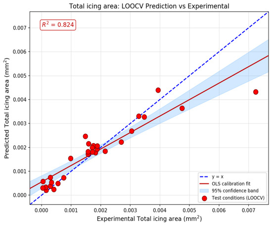
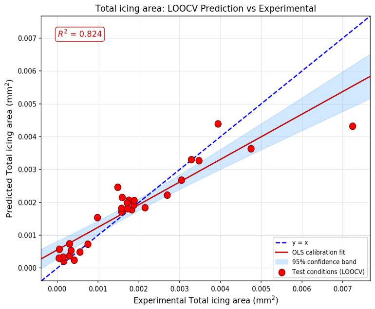
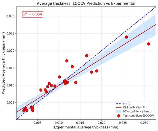
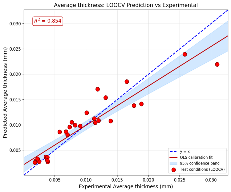
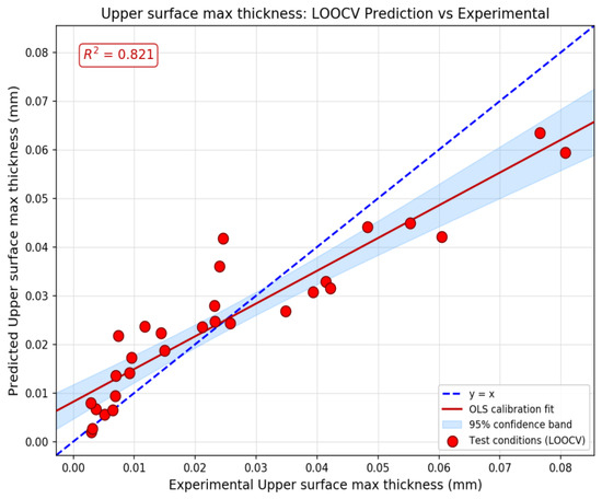
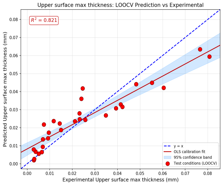
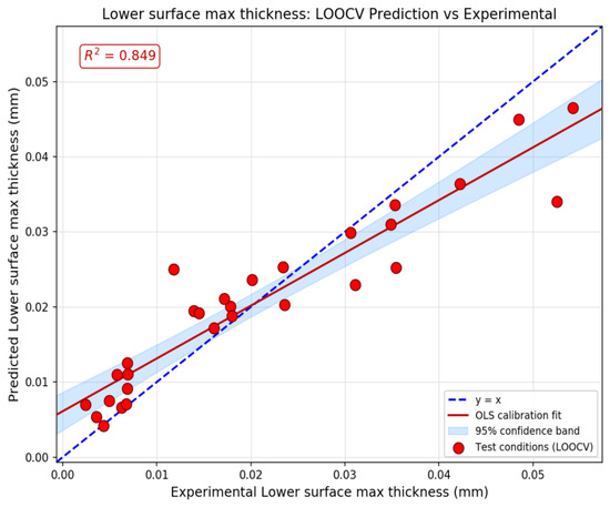
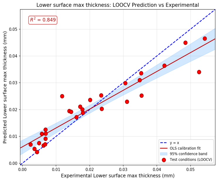
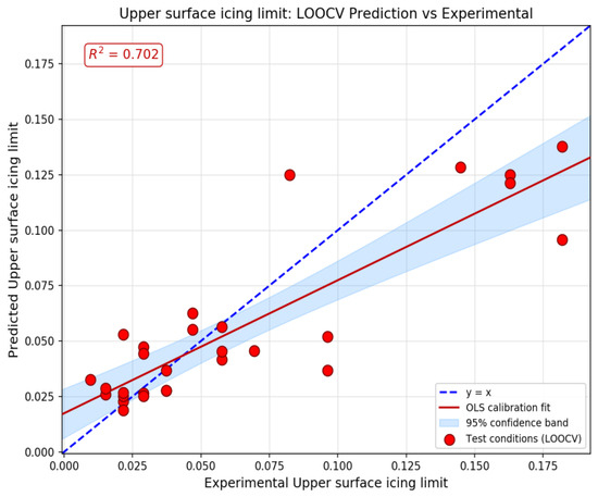
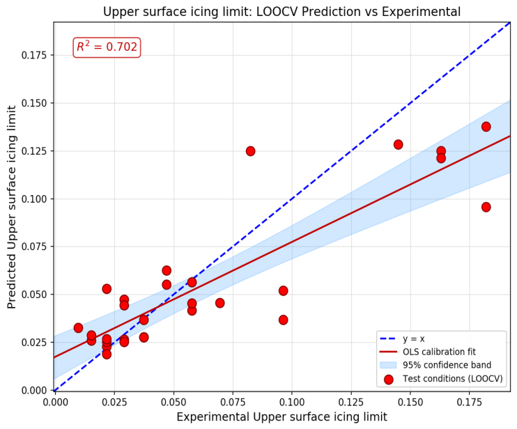
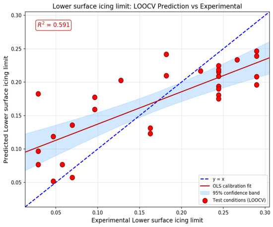
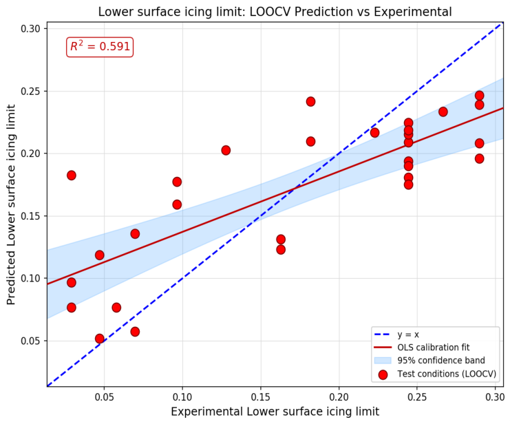
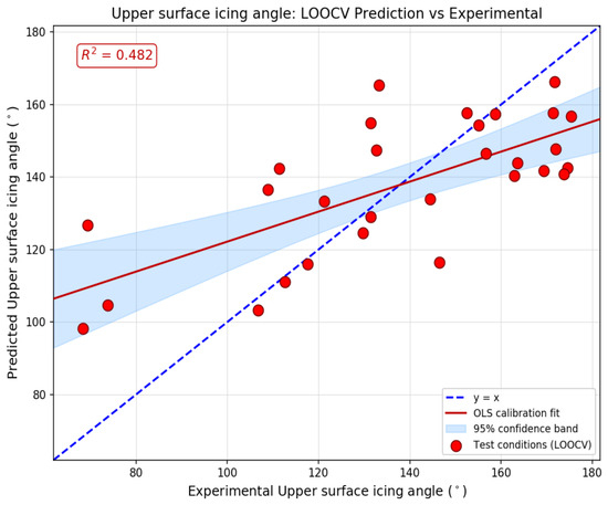
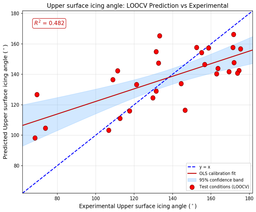
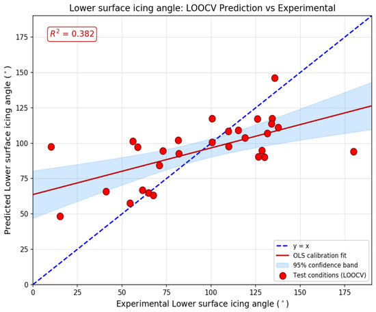
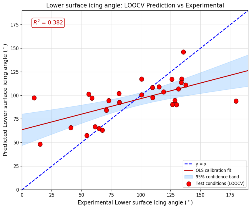
To visually assess the pointwise predictive capability of the improved system for each geometric parameter, Figure 7, Figure 8, Figure 9, Figure 10, Figure 11, Figure 12, Figure 13 and Figure 14 present scatter plots of the LOOCV predicted values versus experimental measurements for all 29 test conditions. In each scatter plot, a least-squares calibration line and its 95% confidence band are also shown to assess the agreement between the predicted and experimental values together with their uncertainty. Overall, the predicted points are tightly clustered around the ideal diagonal line, exhibiting neither monotonic deviation nor structural bias. This confirms that the ridge regression framework, augmented with numerical priors and engineering auxiliary features, effectively corrects the systematic deviations inherent in raw FENSAP-ICE predictions [14,15].

Figure 7. Experimental total area A_total scatter plot.

Figure 8. Experimental average thickness t_avg scatter plot.

Figure 9. Experimental upper surface max thickness t_u scatter plot.

Figure 10. Experimental lower surface max thickness t_l scatter plot.

Figure 11. Experimental upper surface icing limit x_u scatter plot.

Figure 12. Experimental lower surface icing limit x_l scatter plot.

Figure 13. Experimental upper surface icing angle θ_u scatter plot.

Figure 14. Experimental lower surface icing angle θ_l scatter plot.

The prediction robustness of global parameters achieves the most noteworthy performance. For A_total, the scatter points are highly concentrated in the near-diagonal region, with only a single case deviating beyond one standard unit; moreover, the majority of samples aggregate within the first half of the numerical range. The average ice thickness similarly shows only one case with comparable deviation, yet its point cloud distributes more uniformly along the entire diagonal. This indicates that the response of average thickness to varying conditions is more linear than that of total area, and that the numerical prior provided by t_{avg_FEN} has been effectively exploited across the full scale.

The prediction accuracy for local thickness parameters t_u and t_l also remains at a high level. Only two to three cases deviate from the diagonal by more than one standard unit. These deviations all occur in cases with large thickness values, corresponding to SLD conditions with high LWC or long icing time. Under such conditions, enhanced droplet splashing and rebound increase the complexity of the spatial distribution of collection efficiency, thereby amplifying the difficulty of predicting the local maximum thickness. Nevertheless, the predictions remain close to the diagonal for the vast majority of cases, demonstrating that the ridge regression model has captured the local geometric features with engineering-acceptable accuracy under the small-sample constraint.

The scatter distributions of the icing limit parameters x_u and x_l embody the effect of the differentiated modeling strategies adopted in this work. For the upper-surface icing limit x_u, points close to the origin are densely distributed near the diagonal, indicating excellent correction performance for conditions with limited icing extent. As the absolute value of x_u increases, the scatter dispersion gradually enlarges, with the farthest cases exceeding a distance of 2 standard units from the diagonal. This pattern is consistent with the increased experimental uncertainties caused by violent SLD breakup under extreme conditions, and can be regarded as a manifestation of physical limits rather than model failure. For the lower-surface icing limit x_l, the scatter exhibits a distinctive “uniform-deviation” pattern, in which the deviations remain stable within approximately one standard unit over the entire measurement range, and the points are spread evenly along the diagonal, fully covering the interval from zero to the maximum value. The two-stage strategy first isolates the near-zero regime from the finite-ice regime before regression, which keeps the corrected predictions within the physically admissible range and avoids spurious negative or near-zero values. Only one to two cases deviate by more than one standard unit, further confirming the robustness of the ridge correction for x_l prediction.

The scatter structures of the ice horn angle parameters θ_u and θ_l mirror the different formation mechanisms of upper- and lower-surface ice horns. For θ_u, only three samples lie near the origin, while the vast majority of points are located in the latter two-thirds of the data range. The points are relatively evenly distributed on both sides of the diagonal, with a slight preponderance falling below it, suggesting that the improved system exhibits a mild underestimate tendency for the upper-surface ice horn angle. The formation of horn ice strongly depends on the gradient distribution of local collection efficiency and surface runback processes, factors that exhibit considerable randomness under SLD conditions, making prediction of the upper-surface horn angle more challenging than that of other parameters. In contrast, the points for θ_l are highly concentrated in the middle segment of the data range, with few samples at the extremes. The overall deviation is noticeably smaller than that for θ_u, since only three to four cases deviate by more than one standard unit. This conforms to the fact that the lower-surface ice horn is strongly constrained by the lower surface of the airfoil, with a more limited variation range.

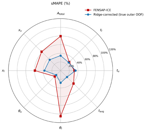
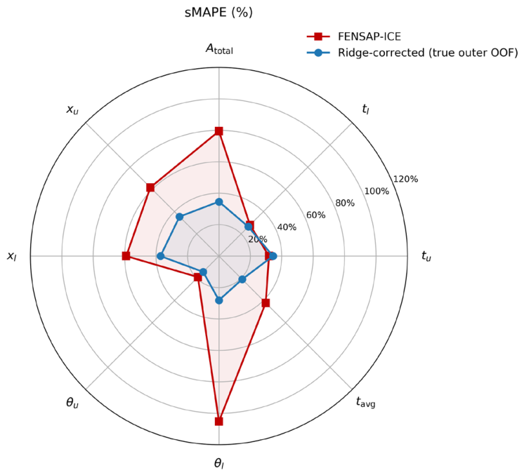
To directly compare the overall performance of the improved system against FENSAP-ICE across all eight parameters, Figure 15 presents a radar chart based on sMAPE. The radar chart clearly illustrates that the improved system substantially outperforms FENSAP on multiple dimensions, including A_total, θ_l, x_u, x_l, and t_avg, with t_u being the only parameter where it is marginally inferior.

Figure 15. Radar chart of sMAPE.

To analyze the contribution of different feature groups to ice shape prediction performance, an ablation study was conducted along three core dimensions, namely local ice thickness, icing extent, and total ice volume. The upper-surface maximum ice thickness t_u, the upper-surface icing limit x_u, and the average ice thickness t_avg were selected as representative geometric parameters, and three feature configurations were designed for comparison.

Configuration M1 constitutes a purely data-driven feature set, employing five original condition parameters AOA, LWC, T, MVD, and t to simulate a modeling scenario completely devoid of numerical simulation priors. Configuration M2 introduces FENSAP numerical prior features by augmenting M1 with the category-relevant geometric parameters predicted by FENSAP-ICE; for t_u, t_{u_FEN}, t_{l_FEN}, and A_{total_FEN} are added; for x_u, x_{u_FEN}, x_{l_FEN}, and associated thickness parameters are added; for t_avg, t_{u_FEN}, t_{l_FEN}, A_{total_FEN}, and t_{avg_FEN} are added. This configuration tests the contribution of the numerical simulation prior knowledge. Configuration M3 is the complete feature set, further incorporating the six domain-knowledge-aided features listed in Table 3 on top of M2.

All configurations shared an identical LOOCV evaluation framework and a unified candidate regularization parameter grid of λ ∈ [10⁻², 10²]. To control for extraneous variables, the feature sets in the ablation study were strictly confined within the category-specific scope of each parameter, with no cross-parameter features introduced, thereby ensuring fairness in the inter-configuration comparison. Table 6 presents the LOOCV-sMAPE results for the three representative parameters under the three feature configurations, with the raw FENSAP-ICE prediction errors serving as a reference baseline.

Table 6. Ablation study results for representative ice shape geometric parameters (LOOCV sMAPE/%).

Model Configuration	tu	xu	tavg
M1	46.68%	54.72%	33.10%
M2	40.97%	50.54%	23.11%
M3	38.96%	49.18%	22.70%

The regularization parameter λ increases monotonically with the number of features. Taking x_u as an example, the λ values for M1, M2, and M3 are 2.81, 3.39, and 4.94, respectively, indicating that the L2 regularization strength must adaptively increase with the feature dimensionality to suppress overfitting.

Comparing M1 against M2 reveals that the purely data-driven M1 configuration performs poorly across all parameters, particularly for x_u and t_u, which yield sMAPE values of 54.72% and 46.68%, respectively. This reflects that, under conditions with only 29 samples, a purely data-driven strategy struggles to capture the nonlinear physical processes characteristic of SLD, such as droplet breakup and splashing. Upon introducing FENSAP-ICE predictions, the prediction accuracy of all three parameters improves substantially; the sMAPE of t_u decreases by 5.71 percentage points, that of x_u by 4.18 percentage points, and t_avg shows the largest reduction, of 10 percentage points. From this, it can be inferred that although FENSAP-ICE possesses systematic biases in SLD icing, its computational model comprehensively integrates information on complex physical processes, including flow field computation, droplet impingement, and icing thermodynamics, rendering its predicted relative trends more correlated with experimental values and thus providing an efficient physical prior for the machine learning model.

When the complete feature set of M3 is adopted, the sMAPE of t_u further drops to 38.96%, that of x_u to 49.18%, and t_avg shows a modest improvement to 22.70%. The marginal gain for t_avg is noticeably smaller than those for t_u and x_u. This is because t_avg, serving as a global statistical quantity, has its variation trend already adequately captured by t_{avg_FEN}, whereas the engineering features in Table 3 are primarily associated with local ice shape characteristics such as the location of maximum thickness and the icing limit; hence, their modulating effect is more pronounced on local parameters than on the global mean.

Moreover, comparing Table 6 with Table 5 reveals that the ablation study values are generally higher. This is because the improved system in Table 5 employs a complete, cross-parameter feature set. For example, in predicting x_u, acknowledging that the extension of the icing limit necessarily accompanies changes in the maximum thickness and that the ice horn position interacts with the upper-/lower-surface asymmetry, the model in Table 5 utilizes not only x_{u_FEN} and x_{l_FEN} but also the full set of eight FENSAP predictions, such as t_{u_FEN}, t_{l_FEN}, A_{total_FEN}, θ_{u_FEN}, θ_{l_FEN}, and θl_FEN, along with the corresponding engineering features. Furthermore, the differentiated modeling strategies for specific parameters such as x_l also contribute additional accuracy gains in the integrated system. The ablation study, in contrast, imposed strict feature-variable control to isolate the independent contributions of each feature group and to reveal the differentiated performance of the engineering features across parameters, resulting in marginally higher numerical values. The numerical comparison between Table 5 and Table 6 demonstrates the effectiveness of the feature design and the modeling strategy proposed in this work.

Extended Validation and Robustness Analysis

This subsection reports three supplementary analyses that assess the generalization of the proposed method and compare it with alternative regression models. To isolate each target variable and to enable a fair comparison across models, these analyses use parameter-specific feature sets, as in the ablation study of Table 6, rather than the integrated cross-parameter feature set of the improved system in Table 5. The cross-parameter feature set is a deliberate design choice of the improved system, because the eight ice-shape parameters are physically coupled and jointly informative; the extended analyses here instead restrict each target to its own feature subset so that the models can be compared on an equal footing. As a consequence, the sMAPE values reported in this subsection are generally higher than, and not directly comparable to, those in Table 5. For example, the standard-LOOCV Ridge sMAPE of the total ice area A_total is 51.78% under the parameter-specific setting of Table 7, whereas the improved system attains 34.65% in Table 5 by exploiting the full cross-parameter feature set; the two figures therefore describe different feature configurations rather than conflicting results. These analyses evaluate the robustness of the correction and the relative performance of the alternative models, and supplement the headline results reported above rather than replace them.

Table 7. Nested cross-validation results compared with standard LOOCV Ridge and the FENSAP-ICE baseline (sMAPE in %; MAE, RMSE and R² reported for the nested estimator).

Parameter	No. of Features	FENSAP sMAPE	Standard LOOCV Ridge sMAPE	Nested CV Ridge sMAPE	Nested MAE	Nested RMSE	FENSAP R2	Nested R2	Nested MaxAE
tu	8	31.86	54.54	54.54	0.00986	0.01359	0.749	0.614	0.03760
tl	8	27.96	34.48	34.48	0.00560	0.00796	0.709	0.729	0.02508
Atotal	8	79.47	51.78	51.78	0.000545	0.000803	0.243	0.748	0.00317
xu	10	61.75	51.08	51.08	0.03198	0.04439	0.058	0.292	0.11368
xl	11	59.00	42.00	42.00	0.06193	0.07842	−0.370	0.285	0.19802
θu	7	18.89	19.40	19.40	25.4082	30.8685	−0.330	0.041	73.5172
θl	7	105.19	35.80	35.80	30.1303	40.4503	−2.977	−0.031	107.4166
tavg	9	42.12	31.53	31.53	0.00279	0.00412	0.435	0.657	0.01204

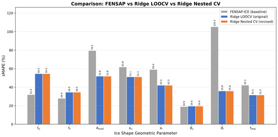
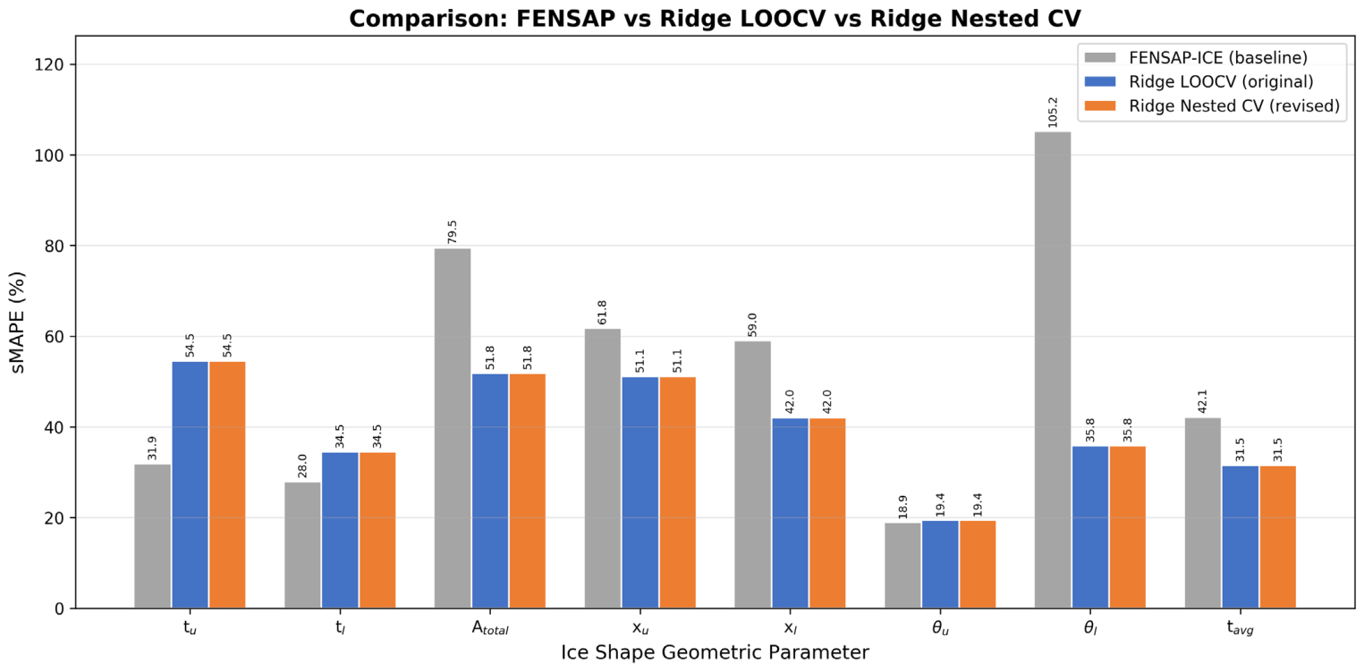
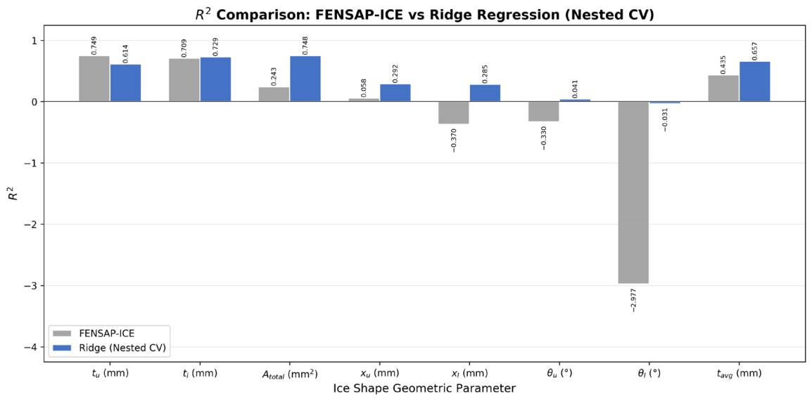
A nested cross-validation is first performed to quantify the optimistic bias of the standard LOOCV evaluation. An inner LOOCV loop selects the regularization parameter, and an outer LOOCV loop estimates the prediction error. Table 7 and Figure 16 compare the nested estimates with the standard LOOCV values, and Figure 17 reports the coefficient of determination of the nested estimator. The nested and standard evaluations yield essentially identical sMAPE for every parameter, confirming that the optimistic bias of the standard LOOCV evaluation is negligible on this dataset.

Figure 16. Standard LOOCV sMAPE versus nested cross-validation sMAPE for each geometric parameter.

Figure 17. R² of the FENSAP-ICE baseline and the nested cross-validation Ridge estimator for each geometric parameter.

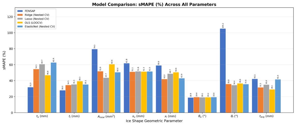
The corrected predictions are then compared with Lasso, ordinary least squares and ElasticNet under the same cross-validation protocol. Table 8 and Figure 18 report the comparison. Ridge remains competitive with or superior to these baselines for the majority of the target parameters.

Table 8. sMAPE comparison (%) among FENSAP-ICE, Ridge, Lasso, OLS and ElasticNet under parameter-specific feature sets. OLS uses outer LOOCV; Lasso and ElasticNet use inner-loop hyperparameter selection.

Parameter	FENSAP	Ridge (Nested CV)	Lasso (Nested CV)	OLS (LOOCV)	ElasticNet (Nested CV)
tu	31.86	54.54	60.67	46.79	62.75
tl	27.96	34.48	35.32	39.33	35.15
Atotal	79.47	51.78	43.65	60.59	50.58
xu	61.75	51.08	51.61	51.35	51.51
xl	59.00	42.00	48.68	50.55	42.91
θu	18.89	19.40	19.08	19.16	19.36
θl	105.19	35.80	34.40	36.57	35.62
tavg	42.12	31.53	35.02	29.06	41.62

Figure 18. sMAPE comparison of FENSAP-ICE and the linear baseline models for each geometric parameter.

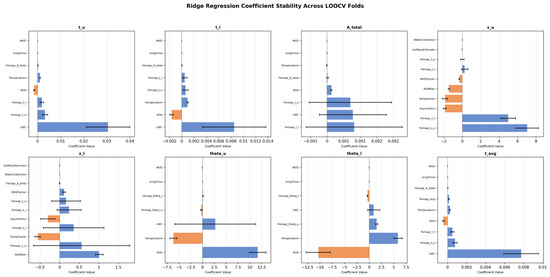
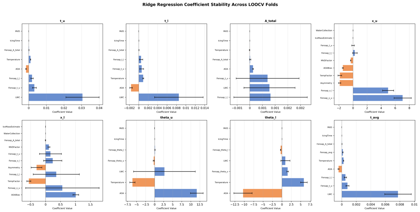
The stability of the ridge coefficients is further examined across the 29 cross-validation folds. Table 9 and Figure 19 report the mean, standard deviation and coefficient of variation (CV) of the coefficients. For the majority of the parameters, and in particular for t_u, t_l and t_avg, the coefficients retain consistent signs and only moderate magnitude variability, with CV values well below unity across the folds. For several other parameters, however, individual coefficients vary markedly between folds: the CV exceeds unity for several FENSAP-prior coefficients of A_total, x_u and x_l and for the LWC coefficient of θ_u, so that even the sign of these particular coefficients is not guaranteed to be stable. The sign and magnitude of such high-CV coefficients should therefore be interpreted with caution, and the physical interpretation of the model rests mainly on the stable coefficients.

Table 9. Mean, standard deviation and coefficient of variation (CV) of the Ridge coefficients across the 29 LOOCV training folds.

Parameter	Feature	Mean Coefficient	Std. Deviation	CV
tu	tu_FEN	0.00324316	0.00113499	0.350
tu	tl_FEN	0.00190622	0.000727374	0.382
tu	Atotal_FEN	0.000160716	5.67235 × 10−5	0.353
tu	t	3.64498 × 10−5	1.87287 × 10−6	0.051
tu	T	0.00105982	0.000102715	0.097
tu	LWC	0.0305328	0.00941314	0.308
tu	MVD	−2.76378 × 10−5	3.2838 × 10−6	0.119
tu	AOA	−0.00152191	0.000200265	0.132
tl	tu_FEN	0.000625228	0.000405528	0.649
tl	tl_FEN	0.000490846	0.000362376	0.738
tl	Atotal_FEN	3.29528 × 10−5	2.20919 × 10−5	0.670
tl	t	2.94183 × 10−5	5.86067 × 10−7	0.020
tl	T	0.000939225	0.000117174	0.125
tl	LWC	0.00851715	0.0051647	0.606
tl	MVD	−1.82865 × 10−5	1.82487 × 10−6	0.100
tl	AOA	−0.00165485	0.000271978	0.164
Atotal	tu_FEN	0.000703001	0.00124144	1.766
Atotal	tl_FEN	0.000819386	0.00144947	1.769
Atotal	Atotal_FEN	1.72882 × 10−5	2.98998 × 10−5	1.729
Atotal	t	3.39756 × 10−6	1.45488 × 10−7	0.043
Atotal	T	−6.72556 × 10−6	1.18264 × 10−5	1.758
Atotal	LWC	0.000779612	0.00100947	1.295
Atotal	MVD	−2.81862 × 10−7	3.29793 × 10−7	1.170
Atotal	AOA	0.000131175	1.94093 × 10−5	0.148
xu	xu_FEN	7.06401	1.22777	0.174
xu	xl_FEN	4.99098	0.79186	0.159
xu	tu_FEN	0.0108733	0.194647	17.901
xu	tl_FEN	0.265637	0.333722	1.256
xu	WaterCollection	−6.82843 × 10−5	0.00013352	1.955
xu	TempFactor	−1.88008	0.269934	0.144
xu	MVDFactor	−0.326325	0.0395391	0.121
xu	AOABias	−1.45384	0.0735433	0.051
xu	Asymmetry	−1.8967	0.159188	0.084
xu	IceMassEstimate	−0.00568724	0.000765755	0.135
xl	xu_FEN	0.562755	1.22746	2.181
xl	xl_FEN	0.241903	0.306978	1.269
xl	tu_FEN	0.165578	0.36725	2.218
xl	tl_FEN	0.359471	0.771432	2.146
xl	Atotal_FEN	−0.00209722	0.00813786	3.880
xl	WaterCollection	0.00127602	0.000201932	0.158
xl	TempFactor	−0.559932	0.0669592	0.120
xl	MVDFactor	0.114662	0.0308536	0.269
xl	AOABias	1.01125	0.0968068	0.096
xl	Asymmetry	−0.301689	0.181063	0.600
xl	IceMassEstimate	−0.000561475	0.00131155	2.336
θu	θu_FEN	−0.268808	0.160599	0.597
θu	θl_FEN	0.0944212	0.0396762	0.420
θu	t	0.0247478	0.00415572	0.168
θu	T	−6.1513	0.735405	0.120
θu	LWC	2.7166	8.54542	3.146
θu	MVD	−0.0224783	0.0057302	0.255
θu	AOA	11.6663	1.75862	0.151
θl	θu_FEN	1.53404	0.226655	0.148
θl	θl_FEN	−0.343094	0.0548118	0.160
θl	t	0.0224048	0.0038716	0.173
θl	T	5.84577	0.891162	0.152
θl	LWC	0.93248	1.21959	1.308
θl	MVD	0.0156048	0.00970757	0.622
θl	AOA	−10.3365	2.44061	0.236
tavg	tu_FEN	0.000797442	0.000211046	0.265
tavg	tl_FEN	0.000513737	0.000159238	0.310
tavg	Atotal_FEN	3.65087 × 10−5	9.72663 × 10−6	0.266
tavg	tavg_FEN	0.000154444	4.60984 × 10−5	0.298
tavg	t	1.35937 × 10−5	5.88724 × 10−7	0.043
tavg	T	0.000252949	3.29135 × 10−5	0.130
tavg	LWC	0.00774578	0.0018302	0.236
tavg	MVD	−5.83082 × 10−6	8.83428 × 10−7	0.152
tavg	AOA	−0.000452764	7.89832 × 10−5	0.174

Figure 19. Mean and standard deviation of the Ridge coefficients across the 29 LOOCV training folds.

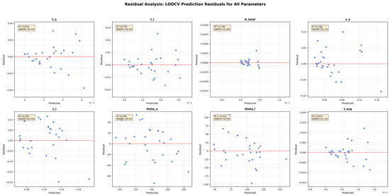
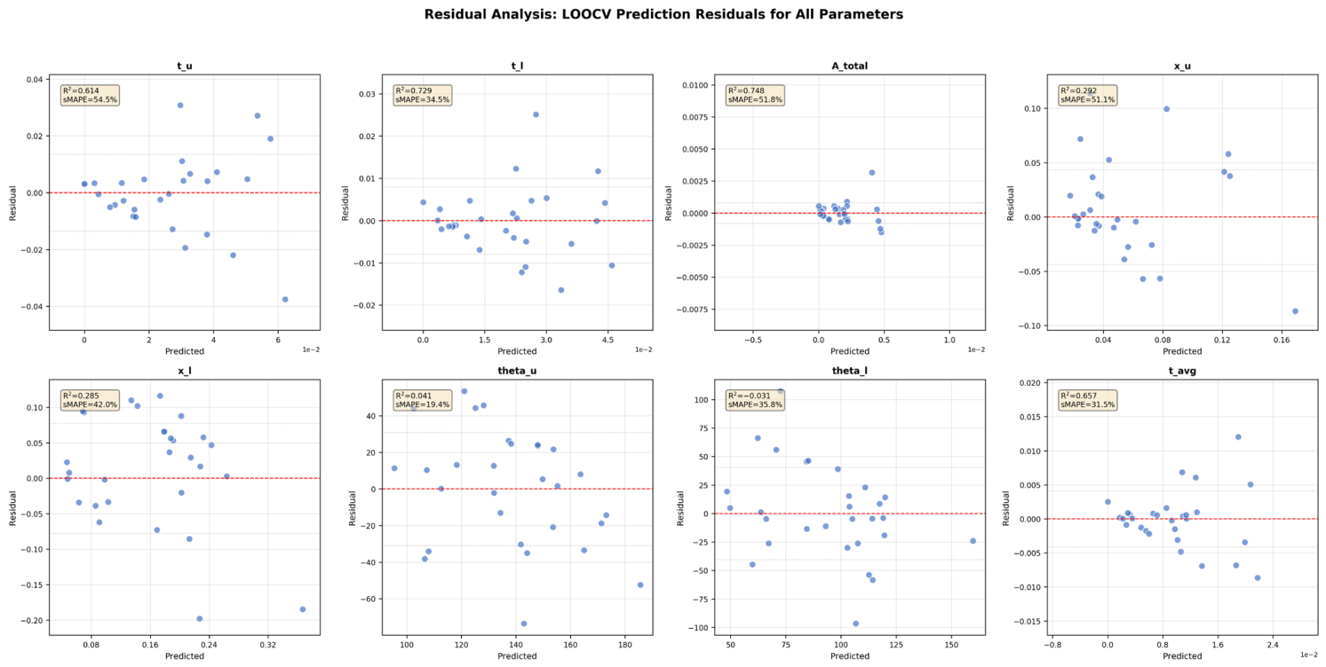
Figure 20 presents a residual analysis of the ridge predictions for the representative geometric parameters. The residuals are scattered around zero without pronounced structure.

Figure 20. Residual analysis of the Ridge predictions (residuals versus fitted values) for the representative geometric parameters.

The supplementary analyses confirm the robustness of the proposed correction on the present dataset. The nested cross-validation reproduces the LOOCV trends with only a small optimism gap, Ridge regression remains competitive with or superior to the Lasso, OLS and ElasticNet baselines for the majority of the target parameters, and the majority of the ridge coefficients retain consistent signs across the folds, while a minority exhibit substantial magnitude variability and should be interpreted with caution.

The above conclusions are constrained by the limited range of the experimental parameters covered. Velocity takes only two levels, 61 and 95 m/s, each coupled with a fixed pressure and temperature, so the isolated velocity effect cannot be separated from the coupled conditions. The median volumetric diameter is clustered at four levels, 19, 20, 110 and 526 μm, and only the NACA0012 geometry is considered. The proposed SLD ice-shape prediction model and its reported accuracy are therefore applicable only within the parameter ranges covered by the present dataset.

4. Conclusions

Addressing the systematic bias in numerical icing simulations under supercooled large droplet conditions, this paper proposes an improved ice shape prediction system based on ridge regression and physical priors. Evaluated via leave-one-out cross-validation on 29 sets of NACA0012 airfoil icing wind tunnel experimental data, the principal conclusions are as follows:

(1)

The introduction of numerical priors is the primary performance driver; ablation experiments indicate that it reduces the average ice thickness prediction error by approximately 10 percentage points. The six engineering auxiliary features built upon this foundation can further reduce the error of local ice shape parameters, such as the upper-surface maximum thickness, by approximately 2 percentage points. The two components realize baseline correction and local refinement, respectively.

(2)

Compared with the raw FENSAP-ICE predictions, the improved system reduces the sMAPE of every key parameter, from 79.47% to 34.65% for the total ice area A_total, from 105.19% to 28.08% for the lower-surface ice horn angle θ_l, from 61.75% to 35.48% for the upper-surface icing limit x_u, from 59.00% to 37.21% for the lower-surface icing limit x_l, and from 42.12% to 20.89% for the average ice thickness t_avg.

(3)

This study is constrained by the limited number of experimental samples and the covered range of velocity conditions; the evaluation may contain an optimistic bias. Future work will expand the data scale, introduce uncertainty quantification, and explore features that more directly capture the microphysical processes characteristic of SLD.

(4)

Through nested cross-validation, comparison with alternative linear baselines, and coefficient-stability analysis, the robustness of the proposed correction is confirmed. The nested evaluation shows only a small optimism gap; the correction remains competitive with the baselines for most target parameters, and the majority of the ridge coefficients retain consistent signs across the folds, while a minority show substantial magnitude variability and should be interpreted with caution.

(5)

By correcting the icing limits and total ice area, the proposed method mitigates the risk of undersized ice protection regions inherent in the raw FENSAP-ICE predictions. Since the correction is a computationally inexpensive post-processing step, it can be embedded directly into existing icing-simulation workflows and is therefore well suited to the preliminary design of aircraft anti-icing and de-icing systems.

References

- Lynch, F.T.; Khodadoust, A. Effects of ice accretions on aircraft aerodynamics. Prog. Aerosp. Sci. 2001, 37, 669–767. [Google Scholar] [CrossRef] [Scilit]
- Tan, S.C.; Papadakis, M. Droplet Breakup, Splashing and Re-Impingement on An Iced Airfoil. In Proceedings of the 4th AIAA Theoretical Fluid Mechanics Meeting, Toronto, ON, Canada, 6–9 June 2005. [Google Scholar]
- Honsek, R.; Habashi, W.G.; Aubé, M.S. Eulerian modeling of in-flight icing due to supercooled large droplets. J. Aircr. 2008, 45, 1290–1296. [Google Scholar] [CrossRef] [Scilit]
- Broeren, A.P.; Potapczuk, M.G.; Riley, J.T.; Villedieu, P.; Moens, F.; Bragg, M. Swept-wing ice accretion characterization and aerodynamics. AIAA J. 2015, 53, 2986–3003. [Google Scholar]
- Beaugendre, H.; Morency, F.; Habashi, W.G. FENSAP-ICE’s three-dimensional in-flight ice accretion module: ICE3D. J. Aircr. 2003, 40, 239–247. [Google Scholar] [CrossRef] [Scilit] [PubMed]
- Habashi, W.G. Recent advances in CFD for in-flight icing simulations. J. Jpn. Soc. Fluid Mech. 2009, 28, 99–118. [Google Scholar]
- Papadakis, M.; Rachman, A.; Wong, S.C.; Yeong, H.-W.; Hung, K.E.; Vu, G.T.; Bidwell, C.S. Water Droplet Impingement on Simulated Glaze, Mixed, and Rime Ice Accretions; NASA/CR-2007-213961; NASA: Washington, DC, USA, 2007.
- Hu, Y.; Pan, J.; Liu, Y.; Zhang, C.; Jiang, Y.; Zhu, J. Research on icing model and calculation methods. Phys. Fluids 2024, 36, 093334. [Google Scholar] [CrossRef] [Scilit]
- Chang, S.; Leng, M.; Wu, H.; Thompson, J. Aircraft ice accretion prediction using neural network and wavelet packet transform. Aircr. Eng. Aerosp. Technol. 2016, 88, 128–136. [Google Scholar] [CrossRef] [Scilit]
- Li, S.; Qin, J.; He, M.; Paoli, R. Fast evaluation of aircraft icing severity using machine learning based on XGBoost. Aerospace 2020, 7, 36. [Google Scholar] [CrossRef] [Scilit]
- Pan, P.; Xue, M.; Zhang, Y.; Ni, Z.; Wang, Z. Study on Quantitative Prediction Scheme of Aircraft Icing Based on Random Forest Algorithm. J. Environ. Account. Manag. 2023, 11, 329–339. [Google Scholar] [CrossRef] [Scilit]
- Strijhak, S.; Ryazanov, D.; Koshelev, K.; Ivanov, A. Neural network prediction for ice shapes on airfoils using iceFoam simulations. Aerospace 2022, 9, 96. [Google Scholar] [CrossRef] [Scilit]
- Dong, Y. An application of Deep Neural Networks to the in-flight parameter identification for detection and characterization of aircraft icing. Aerosp. Sci. Technol. 2018, 77, 34–49. [Google Scholar] [CrossRef] [Scilit]
- He, L.; Qian, W.Q.; Yi, X.; Wang, Q.; Zhang, X. Graphical prediction method of airfoil ice shape based on transposed convolution neural networks. J. Natl. Univ. Def. Technol. 2021, 43, 98–106. (In Chinese) [Google Scholar] [CrossRef]
- Xu, Z.K.; Dai, H.; Zhang, H.J. Deep Learning–Based Method for Efficient Airfoil Rime Icing Prediction. J. Aerosp. Eng. 2025, 38, 04025081. [Google Scholar] [CrossRef] [Scilit]
- Carleo, G.; Cirac, I.; Cranmer, K.; Daudet, L.; Schuld, M.; Tishby, N.; Vogt-Maranto, L.; Zdeborová, L. Machine learning and the physical sciences. Rev. Mod. Phys. 2019, 91, 045002. [Google Scholar] [CrossRef] [Scilit]
- Kutz, J.N. Deep learning in fluid dynamics. J. Fluid Mech. 2017, 814, 1–4. [Google Scholar] [CrossRef] [Scilit]
- Abdelghany, E.S.; Farghaly, M.B.; Almalki, M.M.; Sarhan, H.H.; Essa, M.E.-S.M. Machine Learning and IoT Trends for Intelligent Prediction of Aircraft Wing Anti-Icing System Temperature. Aerospace 2023, 10, 676. [Google Scholar] [CrossRef] [Scilit]
- Cardona, A.; Nakouri, H.; Brassard, J.D.; Momen, G. Machine learning prediction of aircraft anti-icing fluid endurance: A comparative study using natural and artificial snow data. Aerosp. Sci. Technol. 2026, 176, 112103. [Google Scholar] [CrossRef] [Scilit]
- Kallarappayi, A.; Nixon, J.D.; Bégin-Drolet, A.; Godreau, C. Machine- and deep-learning models for wind turbine icing prediction across multiple horizons: The influence of ice sensors and weather forecasts. Cold Reg. Sci. Technol. 2026, 248, 104940. [Google Scholar] [CrossRef] [Scilit]
- Raissi, M.; Perdikaris, P.; Karniadakis, G.E. Physics-informed neural networks: A deep learning framework for solving forward and inverse problems involving nonlinear partial differential equations. J. Comput. Phys. 2019, 378, 686–707. [Google Scholar] [CrossRef] [Scilit]
- Ling, J.; Kurzawski, A.; Templeton, J. Reynolds averaged turbulence modelling using deep neural networks with embedded invariance. J. Fluid Mech. 2016, 807, 155–166. [Google Scholar] [CrossRef] [Scilit]
- Wang, Z.G.; Li, T.; Zheng, W.Z.; Wang, Y.; Hou, H.; Lin, X. Physics knowledge guided iterative self-transfer learning for icing prediction. Power Syst. Prot. Control 2025, 53, 95–105. (In Chinese) [Google Scholar] [CrossRef]
- Chen, H.; He, L.; Qian, W.Q.; Wang, S. Multiple aerodynamic coefficient prediction of airfoils using a convolutional neural network. Symmetry 2020, 12, 544. [Google Scholar] [CrossRef] [Scilit]
- SAE International. Icing Wind Tunnel Interfacility Comparison Tests; Aerospace Information Report AIR5666; SAE Aerospace: Warrendale, PA, USA, 2012. [Google Scholar]
Disclaimer/Publisher’s Note: The statements, opinions and data contained in all publications are solely those of the individual author(s) and contributor(s) and not of MDPI and/or the editor(s). MDPI and/or the editor(s) disclaim responsibility for any injury to people or property resulting from any ideas, methods, instructions or products referred to in the content. |
© 2026 by the authors. Licensee MDPI, Basel, Switzerland. This article is an open access article distributed under the terms and conditions of the Creative Commons Attribution (CC BY) license.