Quasi-Self-Motion-Based Singularity Avoidance for Free-Floating Space Robots

Abstract

We propose a novel singularity-avoidance method for continuous path planning that maintains zero path-tracking error of a non-redundant free-floating space robot (FFSR). Singularities are a major challenge in the path planning of space robots and may lead to the failure of end-effector tracking tasks. First, the singularity characteristics of FFSRs are analyzed, and a numerical method for calculating singularity surfaces is developed. The symmetry properties of the singular surface are further investigated. Subsequently, based on the nonholonomic characteristics of FFSRs, the existence of quasi-self-motion is demonstrated. A quasi-self-motion-based singularity-avoidance method is then proposed for continuous end-effector pose tracking. In addition, the workspace regions where quasi-self-motion does not exist are analytically derived. Numerical simulations verify the effectiveness of the proposed method. Compared with existing singularity-avoidance approaches, the proposed method achieves accurate path tracking while enabling both active singularity avoidance and singularity escape.

1. Introduction

In recent years, space robots have been increasingly applied in on-orbit servicing missions, including space debris removal [1,2,3], on-orbit assembly and maintenance [4,5], and on-orbit refueling [6]. Path planning is one of the key technologies supporting these missions. The robotic system investigated in this paper consists of a manipulator mounted on a satellite base. To reduce unnecessary internal disturbances and minimize propellant consumption, the free-floating mode, in which neither the position nor the attitude of the base is actively controlled, is generally regarded as the most desirable operating mode [7,8]. Compared with fixed-base manipulators, the free-floating space robots (FFSRs) operate without external forces or torques and are therefore subject to momentum and angular momentum conservation laws. In particular, angular momentum conservation introduces a non-integrable nonholonomic constraint, which significantly increases the complexity of the system kinematics [9,10]. Moreover, the kinematic behavior of the system becomes strongly coupled with dynamic parameters such as mass and inertia, making path planning substantially more challenging than that of conventional fixed-base manipulators.

Singularities remain a fundamental challenge in robotic path planning. When the desired motions are directly specified in joint space, only forward kinematics is required, and singularity problems do not arise [11]. In practical application, however, desired paths are usually specified in end-effector pose space. In this case, inverse kinematics must be employed, and the system may reach singular configuration in which the end-effector loses motion capability along certain direction, thereby leading to path-tracking failure [12]. Due to the unique kinematic characteristics of FFSRs, their singularity properties differ significantly from those of conventional fixed-base manipulators, and many existing singularity-avoidance methods cannot be directly applied to space robotic systems [13].

The singularity analysis of FFSRs is generally established within the framework of the generalized Jacobian matrix (GJM), which explicitly incorporates the dynamic coupling between the manipulator and the floating base into the kinematic mapping [10]. A singularity occurs when the GJM becomes rank deficient [14]. Previous studies have shown that FFSRs exhibit not only conventional kinematic singularities but also dynamic singularities caused by the system mass distribution and dynamic coupling effects [15]. Parameters such as the base-to-manipulator mass ratio, inertia distribution, and link mass distribution significantly affect the spatial distribution of dynamic singularities. These singularities severely restrict the reachable workspace and reduce system manipulability, thereby introducing additional constraints into path planning [16]. Furthermore, the dynamic singularities are not solely determined by the instantaneous geometric configuration of the manipulator. Instead, they exhibit path-dependent characteristics due to the nonholonomic nature of the system [17,18]. Specifically, the angular momentum conservation constraint introduces strong dynamic coupling between the base and the manipulator, causing identical end-effector poses to correspond to different singular configurations depending on the motion path used to reach them.

In robot path planning, depending on how the task is specified, there are two main categories: point-to-point planning and continuous path planning [19]. Point-to-point planning specifies only the initial and final end-effector poses, whereas continuous path planning constrains the entire motion path of the end-effector. Existing singularity-avoidance methods for FFSRs are mainly derived from approaches originally developed for fixed-base manipulators. For point-to-point planning problem, parameterized joint trajectories combined with optimization algorithms have been employed to search feasible joint-space paths without explicitly solving inverse kinematics, thereby reducing the possibility of reaching singular configurations [20,21]. Gradient-based methods and reinforcement learning approaches have also been proposed to guide the system toward target poses through regions with relatively high singularity measures in Cartesian space [22,23]. Since singular regions usually occupy only a small portion of the workspace and point-to-point planning does not constrain intermediate path, feasible singularity-free paths can often be obtained without significant difficulty. Continuous path planning is more practical in engineering applications and considerably more challenging. Existing methods mainly rely on robust pseudo-inverse techniques. Early studies replaced the GJM with the Jacobian matrix of fixed-base manipulators to reduce the probability of encountering singularities during path tracking [24]. Subsequently, robust pseudo-inverse methods introduced damping terms into the pseudo-inverse calculation of the GJM to maintain joint-velocity stability near singularities [25,26]. Adaptive damping strategies and genetic-algorithm-based parameter optimization have also been developed to improve performance. Although robust pseudo-inverse methods maintain the solvability of inverse kinematics near singularities, they fundamentally rely on sacrificing tracking accuracy by introducing path-tracking errors. Moreover, these methods do not actively drive the system away from singular configurations. To address this limitation, a time-scaling strategy has been proposed to slow down motion when the system passes through singular regions. This approach ensures path tracking accuracy to the greatest possible extent [27,28]. However, the trade-off is a relatively large velocity tracking error. The more severe the singularity, the smaller the time scale must be, which in turn results in a longer additional time required. When the system becomes completely trapped in a singularity, the additional time approaches infinity, meaning that path planning can no longer be completed at that point. For space robots with redundant degrees of freedom, null-space-based self-motion methods have been widely used for singularity avoidance [29,30]. These methods exploit redundant degrees of freedom to reconfigure the manipulator within the Jacobian null space without affecting the end-effector pose, enabling the robot to avoid or escape singular configurations while maintaining accurate path tracking. However, such methods are not applicable to non-redundant systems because these systems do not possess nontrivial null spaces or conventional self-motion capabilities.

Although existing singularity avoidance methods can effectively maintain the solvability of inverse kinematics near singular configurations, most of them inevitably introduce deviations between the desired and actual end-effector trajectories or lack the capability of actively escaping from singular configurations. In contrast, the proposed quasi-self-motion-based method exploits the nonholonomic characteristics of free-floating space robots and enables configuration adjustment while preserving the desired end-effector pose trajectory. The main contributions of this work are summarized as follows:

• A novel quasi-self-motion concept is introduced for non-redundant free-floating space robots, where closed-loop end-effector motions are utilized to modify joint configurations without introducing path-tracking errors.
• The existence mechanism of quasi-self-motion is theoretically analyzed based on the non-integrability of angular momentum conservation constraints.
• A singularity avoidance framework is developed that simultaneously achieves zero end-effector tracking error and active singularity escape capability.

The limitation of this method is that the insertion of quasi-self-motion prolongs the time required to reach the target pose. Consequently, it is not applicable to path planning problems for non-cooperative targets whose target poses are not fixed or even unpredictable.

The paper is structured as follows. Section 2 establishes the dynamic and kinematic models of a three-degree-of-freedom (3-DOF) planar FFSR and introduces the continuous path-planning framework. Section 3 analyzes system singularity characteristics and presents the associated theoretical proofs. Section 4 calculates and visualizes singularity surfaces in joint space. Section 5 presents the proposed quasi-self-motion-based singularity-avoidance method. Section 6 provides numerical simulations to verify its effectiveness. Finally, Section 7 concludes the paper and outlines future work.

2. Modeling and Singularity Description

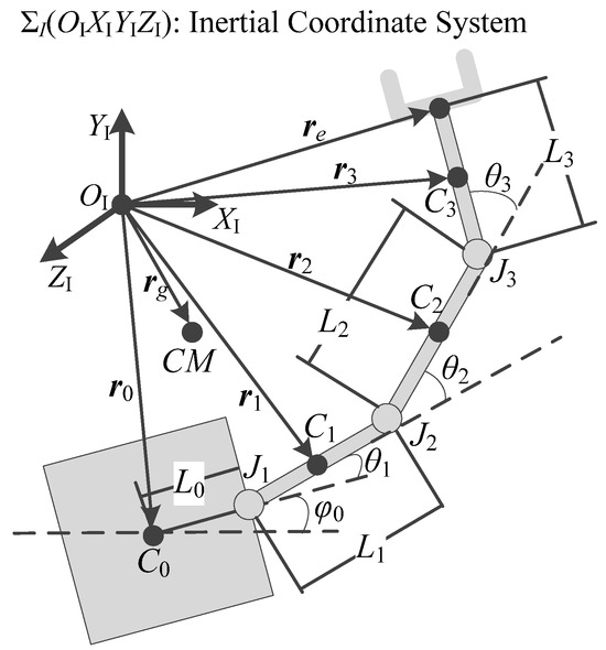
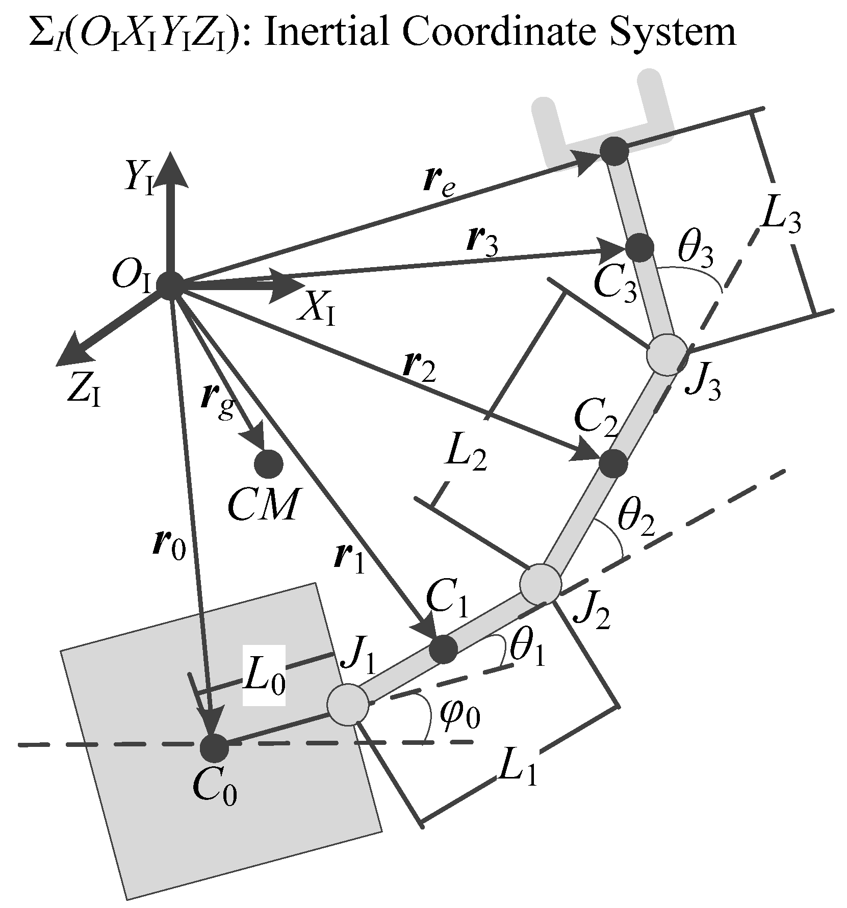
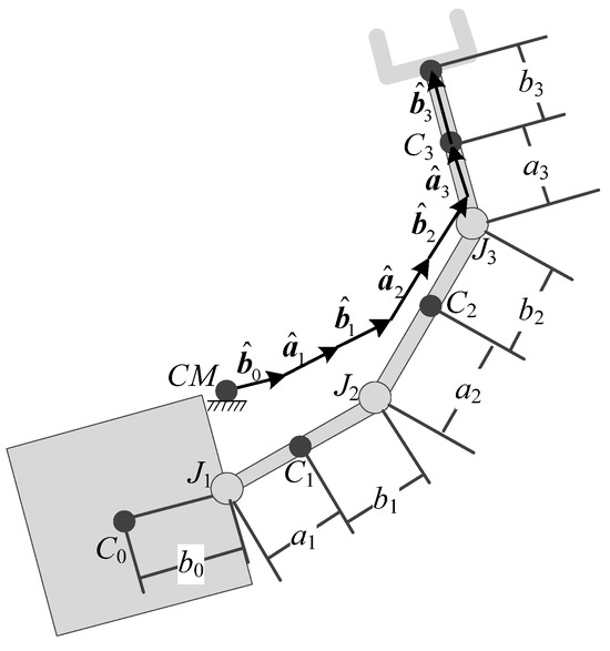
This paper investigates a single-arm FFSR with no redundant degrees of freedom. To simplify calculations and focus on the algorithm itself, a planar 3-DOF robot, as shown in Figure 1, is selected as the subject of study. ${\Sigma }_I$ is the inertial coordinate system, and its degrees of freedom consist of translation in the $X_{\mathrm{I}}\text{-}{Y}_{\mathrm{I}}$ plane and rotation about the $Z_{\mathrm{I}}$-axis. The FFSR system consists of a base $B_0$ and linkages $B_1$, $B_2$, and $B_3$, denoted as components $B_j$ (j = 0, 1, 2, 3). Linkages $B_1$, $B_2$, and $B_3$ are collectively referred to as the manipulator; the center of mass of component $B_j$ is $C_j$, and a body-fixed coordinate system ${\Sigma }_j$ is rigidly attached at the center of mass, with the $Z_j$-axis aligned with the $Z_I$ direction; The mass of component $B_j$ is $m_j$, and its moment of inertia about the $Z_j$-axis is $I_j$; the inner joint of link $B_j$ (j = 1, 2, 3) is $J_j$, and the outer joint is $J_{j+1}$; the length of link j is $L_j$; $c_{j,1}$ and $c_{j,2}$ are the normalized lengths of $\overline{J_j{C}_j}$ and $\overline{C_j{J}_{j+1}}$, respectively, satisfying $c_{j,1}+c_{j,2}=1$; The length of $\overline{C_0{J}_1}$ is $L_0$. Let the position vectors of the system’s center of mass, the manipulator’s end-effector, and the component’s center of mass, as well as $\overrightarrow{J_j{C}_j}$, $\overrightarrow{C_j{J}_{j+1}}$, and $\overrightarrow{J_j{J}_{j+1}}$, be denoted by ${\mathit{r}}_{\mathrm{g}}$, ${\mathit{r}}_{\mathrm{e}}$, ${\mathit{r}}_j$, ${\mathit{a}}_j$, ${\mathit{b}}_j$, and ${\mathit{L}}_j$, respectively. The base attitude angle and the joint angle of $J_j$ are denoted by ${\phi }_0$ and ${\theta }_j$, respectively. The following assumptions are made during the modeling process:

Figure 1. General model of a 3-DOF planar FFSR.

• The system is free from external forces and moments, satisfies the conservation of linear and angular momentum, and has zero initial linear and angular momentum;
• There is one controlled rotational degree of freedom between adjacent links, but the base attitude is not directly controlled.

In the path planning of an FFSR, the objective variables are the end-effector pose of the manipulator, while the control variables are the joint angles. Due to the non-integrable constraint of angular momentum conservation, an FFSR is a nonholonomic system. Consequently, it cannot solve for the joint angles using position-level kinematics; instead, it must solve them indirectly by integrating the results of velocity-level kinematic planning. Therefore, the goal of system modeling is to establish velocity-level kinematic equations.

The attitude angles, attitude angular velocities, center of mass position and velocity vector of component j in the inertial frame ${\Sigma }_I$ are:

$${\phi }_j={\phi }_0+{\displaystyle \sum _{i=1}^j{\theta }_i},$$

(1)

$${\omega }_j\mathit{k}={\omega }_0\mathit{k}+{\displaystyle {\displaystyle \sum _{i=1}^j}{\dot{\theta }}_i\mathit{k}},$$

(2)

$${\mathit{r}}_j={\mathit{r}}_0+{\mathit{b}}_0+{\displaystyle \sum _{i=1}^{j-1}\left({\mathit{a}}_i+{\mathit{b}}_i\right)}+{\mathit{a}}_j,$$

(3)

$${\mathit{v}}_j={\dot{\mathit{r}}}_j={\mathit{v}}_0+{\omega }_0\mathit{k}\times {\mathit{r}}_{0j}+{\displaystyle {\displaystyle \sum _{i=1}^j}\left({\dot{\theta }}_i\mathit{k}\times {\mathit{a}}_{i~j}\right)},$$

(4)

In the equation, ${\mathit{a}}_{i~j}=\left({\displaystyle \sum _{k=i}^{j-1}\left({\mathit{a}}_k+{\mathit{b}}_k\right)}\right)+{\mathit{a}}_j$, ${\omega }_0$ is the angular velocity of the base, and $\mathit{k}$ is the unit vector in the $Z_I$-direction. Accordingly, the end-effector pose and velocity can be expressed as:

$${\phi }_{\mathrm{e}}={\phi }_0+{\displaystyle \sum _{i=1}^3{\theta }_i},$$

(5)

$${\omega }_{\mathrm{e}}={\dot{\phi }}_{\mathrm{e}}={\omega }_0+{\displaystyle \sum _{i=1}^3{\dot{\theta }}_i},$$

(6)

$${\mathit{r}}_{\mathrm{e}}={\mathit{r}}_0+{\mathit{b}}_0+{\displaystyle \sum _{i=1}^3\left({\mathit{a}}_i+{\mathit{b}}_i\right)},$$

(7)

$${\mathit{v}}_{\mathrm{e}}={\dot{\mathit{r}}}_{\mathrm{e}}={\mathit{v}}_0+{\omega }_0\mathit{k}\times \left({\mathit{r}}_{\mathrm{e}}-{\mathit{r}}_0\right)+{\displaystyle {\displaystyle \sum _{i=1}^3}\left({\dot{\theta }}_i\mathit{k}\times \left({\mathit{a}}_{i~3}+{\mathit{b}}_3\right)\right)},$$

(8)

The system’s equation for the conservation of angular momentum with respect to $O_I$ is:

$$\mathit{L}={\displaystyle {\displaystyle \sum _{j=0}^3}\left(I_j{\omega }_j\mathit{k}+\left({\mathit{r}}_j\times m_j{\dot{\mathit{r}}}_j\right)\right)=0},$$

(9)

Substituting Equations (2)–(4) into Equation (9), the resultant component about the $Z_I$-axis can be simplified to:

$$L_z=I_{\omega }{\omega }_0+{\mathit{I}}_{\theta }\dot{\mathit{\theta }}=0,$$

(10)

In the equation: $\mathit{\theta }={\left(\begin{array}{ccc}{\theta }_1& {\theta }_2& {\theta }_3\end{array}\right)}^{\mathrm{T}}$ and $\dot{\mathit{\theta }}={\left(\begin{array}{ccc}{\dot{\theta }}_1& {\dot{\theta }}_2& {\dot{\theta }}_3\end{array}\right)}^{\mathrm{T}}$ represent the joint angle vector and the joint angular velocity vector, respectively; ${\mathit{I}}_{\theta }=\left(\begin{array}{ccc}{I}_{\theta 1}& I_{\theta 2}& I_{\theta 3}\end{array}\right)$; and $I_{\omega }$, $I_{\theta 1}$, $I_{\theta 2}$, and $I_{\theta 3}$ are the equivalent moments of inertia about the ${\mathrm{Z}}_{\mathrm{I}}$ axis, which are functions of the base attitude angle ${\phi }_0$ and the joint angles ${\theta }_j$ (j = 1, 2, 3), specifically:

$$\begin{array}{ll}{I}_{\omega }=& \left(I_0+I_1+I_2+I_3\right)-{\mathit{k}}^T\left(m_1{\left({\left({\mathit{r}}_1-{\mathit{r}}_0\right)}^{\times }\right)}^2+m_2{\left({\left({\mathit{r}}_2-{\mathit{r}}_0\right)}^{\times }\right)}^2+\right.\\ & \left. m_3{\left({\left({\mathit{r}}_3-{\mathit{r}}_0\right)}^{\times }\right)}^2\right)\mathit{k}+M{\mathit{k}}^T{\left({\left({\mathit{r}}_g-{\mathit{r}}_0\right)}^{\times }\right)}^2\mathit{k}\end{array},$$

(11)

$$\begin{array}{ll}{I}_{\theta 1}=& \left(I_1+I_2+I_3\right)+{\mathit{k}}^T\left(m_1{\left({\mathit{r}}_g-{\mathit{r}}_1\right)}^{\times }{\mathit{a}}_1^{\times }+m_2{\left({\mathit{r}}_g-{\mathit{r}}_2\right)}^{\times }{\mathit{a}}_{1~2}^{\times }+\right.\\ & \left.m_3{\left({\mathit{r}}_g-{\mathit{r}}_3\right)}^{\times }{\mathit{a}}_{1~3}^{\times }\right)\mathit{k}\end{array},$$

(12)

$$I_{\theta 2}=\left(I_2+I_3\right)+{\mathit{k}}^T\left(m_2{\left({\mathit{r}}_g-{\mathit{r}}_2\right)}^{\times }{\mathit{a}}_2^{\times }+m_3{\left({\mathit{r}}_g-{\mathit{r}}_3\right)}^{\times }{\mathit{a}}_{2~3}^{\times }\right)\mathit{k},$$

(13)

$$I_{\theta 3}=I_3+m_3{\mathit{k}}^T{\left({\mathit{r}}_g-{\mathit{r}}_3\right)}^{\times }{\mathit{a}}_3^{\times }\mathit{k},$$

(14)

Here, $M$ represents the total mass of the system; the system’s center-of-mass vector ${\mathit{r}}_g$ can be calculated using the conservation of total momentum and remains constant during motion; ${( )}^{\times }$ denotes the cross-product matrix operation for 3-dimensional vectors, and is defined as ${\mathit{w}}^{\times }=\left(\begin{array}{ccc}0& -w_3& w_2\\ w_3& 0& -w_1\\ -w_2& w_1& 0\end{array}\right)$ for any vector $\mathit{w}={\left(\begin{array}{ccc}{w}_1& w_2& w_3\end{array}\right)}^T$.

Combining Equations (8) and (10), we can derive the state equation for end-effector pose path planning, where the target variable ${\mathit{X}}_{\mathrm{e}}\left(t\right)=\left(\begin{array}{c}{\phi }_{\mathrm{e}}\left(t\right)\\ {\mathit{r}}_{\mathrm{e}}\left(t\right)\end{array}\right)$ serves as the state variable and the joint angular velocity $\dot{\mathit{\theta }}$ serves as the control variable. This corresponds to the velocity-level kinematic equation for spatial robots [11]:

$${\dot{\mathit{X}}}_{\mathrm{e}}={\mathit{J}}_{\mathrm{g}}\dot{\mathit{\theta }},$$

(15)

In the equation, ${\mathit{J}}_{\mathrm{g}}$ denotes the GJM, whose specific expression is:

$${\mathit{J}}_{\mathrm{g}}=\left(\begin{array}{c}\begin{array}{ccc}\hfill {\displaystyle \frac{I_{\theta 1}}{I_{\omega }}}+1\hfill & \hfill {\displaystyle \frac{I_{\theta 2}}{I_{\omega }}}+1\hfill & \hfill {\displaystyle \frac{I_{\theta 3}}{I_{\omega }}}+1\hfill \end{array}\\ \begin{array}{ccc}\hfill {\mathit{f}}_{1,xy}\hfill & \hfill {\mathit{f}}_{2,xy}\hfill & \hfill {\mathit{f}}_{3,xy}\hfill \end{array}\end{array}\right),$$

(16)

In the equation, ${\mathit{f}}_j$ (j = 1, 2, 3) is the coefficient representing the effect of each link’s rotational motion on the terminal linear velocity; it is a function of the length vectors of each link and the position vector of the system’s center of mass, and is therefore also a function of the base attitude angle ${\phi }_0$ and the joint angles ${\theta }_j$. Specifically:

$${\mathit{f}}_1=-{\left({\mathit{a}}_{1~3}+{\mathit{b}}_3\right)}^{\ast }+{\displaystyle \frac{I_{\theta 1}}{I_{\omega }}}{\left({\mathit{r}}_g-{\mathit{r}}_e\right)}^{\ast }+{\displaystyle \frac{1}{M}}\left(m_1{\mathit{a}}_1^{\ast }+m_2{\mathit{a}}_{1~2}^{\ast }+m_3{\mathit{a}}_{1~3}^{\ast }\right),$$

(17)

$${\mathit{f}}_2=-{\left({\mathit{a}}_{2~3}+{\mathit{b}}_3\right)}^{\ast }+{\displaystyle \frac{I_{\theta 2}}{I_{\omega }}}{\left({\mathit{r}}_g-{\mathit{r}}_e\right)}^{\ast }+{\displaystyle \frac{1}{M}}\left(m_2{\mathit{a}}_2^{\ast }+m_3{\mathit{a}}_{2~3}^{\ast }\right),$$

(18)

$${\mathit{f}}_3=-{\left({\mathit{a}}_3+{\mathit{b}}_3\right)}^{\ast }+{\displaystyle \frac{I_{\theta 3}}{I_{\omega }}}{\left({\mathit{r}}_g-{\mathit{r}}_e\right)}^{\ast }+{\displaystyle \frac{1}{M}}{m}_3{\mathit{a}}_3^{\ast },$$

(19)

In this equation, all vectors are variables in the $X_{\mathrm{I}}\text{-}{Y}_{\mathrm{I}}$ plane of the inertial frame ${\Sigma }_I$, represented as two-dimensional vectors. The symbol ${( )}^{\ast }$ denotes the inverse transformation of this two-dimensional vector, and for any $\mathit{w}={\left(\begin{array}{cc}{w}_1& w_2\end{array}\right)}^T$, it is defined as ${\mathit{w}}^{\ast }={\left(\begin{array}{cc}-w_2& w_1\end{array}\right)}^T$.

Path planning for the end-effector pose of an FFSR is typically performed indirectly using velocity-level kinematic equations, a method known as resolved motion rate control. The approach involves determining the desired end-effector velocity ${\dot{\mathit{X}}}_{\mathrm{e}}\left(t\right)$ based on the desired end-effector pose trajectories, and then calculating the angular velocity commands for each joint of the manipulator using the velocity-level kinematic Equation (15) relating the control variables to the planning objective variables:

$$\dot{\mathit{\theta }}\left(t\right)={\mathit{J}}_{\mathrm{g}}^{+}{\dot{\mathit{X}}}_{\mathrm{e}}\left(t\right),$$

(20)

In the equation: ${\mathit{J}}_{\mathrm{g}}^{+}={\mathit{J}}_{\mathrm{g}}^{\mathrm{T}}{\left({\mathit{J}}_{\mathrm{g}}{\mathit{J}}_{\mathrm{g}}^{\mathrm{T}}\right)}^{-1}$ is the inverse of the GJM.

The resolved motion rate control computes the inverse of the GJM in each planning cycle. Since the GJM is a function of the base attitude and the joint angles, there may be configurations where:

$$\det \left({\mathit{J}}_{\mathrm{g}}{\mathit{J}}_{\mathrm{g}}^{\mathrm{T}}\right)=0,$$

(21)

which causes ${\mathit{J}}_{\mathrm{g}}^{+}$ to be undefined. In a non-redundant FFSR, the dimensions of the control and state variables are equal; in this case, the GJM is a square matrix, and Equation (21) is equivalent to:

$$\det \left({\mathit{J}}_{\mathrm{g}}\right)=0,$$

(22)

A system configuration that satisfies Equations (21) or (22) is referred to as a singular configuration. When the GJM system approaches or reaches a singular configuration, the control commands obtained using the resolved motion rate control will exceed the engineering limits of the physical quantities or even become infinite, rendering the results invalid. Therefore, singular configurations challenges for the end-effector pose path planning, and analyzing the characteristics of singular configurations and taking measures to resolve singularity issues in inverse kinematics have always been of great importance.

3. Singularity Analysis

This chapter analyzes and demonstrates the properties of singularities, laying the groundwork for subsequent work. We present the following conclusions.

Property 1.

Independence of Singularities from Base Attitude: Whether the current state of the FFSR is singular depends on the lengths, masses, and moments of inertia of its individual links, as well as the current joint angles; it is independent of the base attitude.

Proof. 

According to the system singularity calculation Formula (22), it is clear that the singularity is entirely determined by GJM ${\mathit{J}}_{\mathrm{g}}$. From Equations (16)–(19), it is evident that the parameters directly affecting ${\mathit{J}}_{\mathrm{g}}$ are: all link vectors ${\mathit{a}}_j$ and ${\mathit{b}}_j$, and all component masses $m_j$ and moments of inertia $I_j$. Expressing the link vectors ${\mathit{a}}_j$ and ${\mathit{b}}_j$ in the body coordinate system ${\Sigma }_0$ of the base $B_0$ yields the following results:

$${}^0\mathit{b}_0=L_0{\left(\begin{array}{cc}1& 0\end{array}\right)}^T,$$

(23)

$${}^0\mathit{a}_j=c_{j,1}{L}_j{\left(\begin{array}{cc}\cos {\displaystyle \sum _{i=1}^j{\theta }_i}& \sin {\displaystyle \sum _{i=1}^j{\theta }_i}\end{array}\right)}^T \left(j=1,2,3\right),$$

(24)

$${}^0\mathit{b}_j=c_{j,2}{L}_j{\left(\begin{array}{cc}\cos {\displaystyle \sum _{i=1}^j{\theta }_i}& \sin {\displaystyle \sum _{i=1}^j{\theta }_i}\end{array}\right)}^T \left(j=1,2,3\right),$$

(25)

Therefore, ${}^0\mathit{J}_{\mathrm{g}}$, the GJM expressed in the body-fixed coordinate system ${\Sigma }_0$, is a function that depends only on the current joint angles ${\mathit{\theta }}_{cur}$, the link length $L_j$, the mass $m_j$, and the moment of inertia $I_j$, and is independent of the base attitude ${\phi }_0$; that is,

$${}^0\mathit{J}_{\mathrm{g}}={}^0\mathit{J}_{\mathrm{g}}\left({\mathit{\theta }}_{cur},L_j,m_j,I_j\right),$$

(26)

The coordinate transformation matrix from ${\Sigma }_0$ to ${\Sigma }_I$ is a unit orthogonal matrix that depends solely on the base attitude ${\phi }_0$:

$${\mathit{A}}_0^I=\left(\begin{array}{ccc}\cos {\phi }_0& -\sin {\phi }_0& 0\\ \sin {\phi }_0& \cos {\phi }_0& 0\\ 0& 0& 1\end{array}\right),$$

(27)

Combining (26) and (27), we obtain the representation of the GJM in ${\Sigma }_I$ as:

$${\mathit{J}}_{\mathrm{g}}={\mathit{A}}_0^I\left({\phi }_0\right){}^0\mathit{J}_{\mathrm{g}}\left({\mathit{\theta }}_{cur},L_j,m_j,I_j\right),$$

(28)

Clearly, the equation satisfied by the singularities is:

$$\det \left({\mathit{J}}_{\mathrm{g}}\right)=\det \left({\mathit{A}}_0^I\left({\phi }_0\right)\right)\det \left({}^0\mathit{J}_{\mathrm{g}}\left({\mathit{\theta }}_{cur},L_j,m_j,I_j\right)\right)=\det \left({}^0\mathit{J}_{\mathrm{g}}\left({\mathit{\theta }}_{cur},L_j,m_j,I_j\right)\right)=0,$$

(29)

Therefore, the singularity depends only on the current joint angles ${\mathit{\theta }}_{cur}$ and is independent of the base attitude ${\phi }_0$.□

It is worth noting that although the above proof of Property 1 is based on an FFSR model moving in a plane, this property holds for general FFSRs, and the proof can be conducted by analogy with the procedure described above.

It is intuitive that the singularities of an FFSR are independent of the base attitude, i.e., whether the system is singular depends solely on the relative configuration of its internal components, as determined by the joint angles, and is independent of the absolute configuration of the system as a whole in inertial space, as characterized by the base attitude.

4. Calculation of Singular Surface

The singular surface illustrates the spatial distribution of all singularities and serves as an intuitive tool for determining whether a system requires singularity-avoidance operations; it provides direct insights for singularity-avoidance design.

Based on the conclusion of the previous chapter, singularities are primarily determined by the current joint angles; therefore, this paper calculates and plots singular surface in the joint space.

All singularities in the FFSR’s joint space are obtained by solving Equation (22). Due to the highly nonlinear nature of this equation, it is extremely difficult to directly find analytical solutions for all singularities. In this paper, based on Property 1, the base attitude is set to zero, and then the $\det \left({\mathit{J}}_{\mathrm{g}}\right)$ is computed and simplified using the symbolic computation capabilities of automated software, yielding the result:

$$\det \left({\mathit{J}}_{\mathrm{g}}\right)={\displaystyle \frac{M}{N}},$$

(30)

In the equation:

$$M=c_1\sin {\theta }_1+c_2\sin {\theta }_2+c_3\sin \left({\theta }_1+{\theta }_2\right)+c_4\sin \left({\theta }_1-{\theta }_2\right)+c_5\sin \left(2{\theta }_1+{\theta }_2\right),$$

(31)

$$N=d_0+d_1\cos {\theta }_1+d_2\mathrm{co}{\theta }_2+d_3\mathrm{co}{\theta }_3+d_4\cos \left({\theta }_1+{\theta }_2\right)+d_5\cos \left({\theta }_2+{\theta }_3\right)+d_6\cos \left({\theta }_1+{\theta }_2+{\theta }_3\right),$$

(32)

In this equation, $c_i$ ($i=1,2,\cdots ,5$) and $d_i$ ($i=0,1,\cdots ,6$) are scalar parameters determined by the system member length $L_j$, mass $m_j$, and moment of inertia $I_j$. According to Equation (30), the singular equivalence condition is given by:

$$M=0,$$

(33)

Noting that $M$ is a function of only ${\theta }_1$ and ${\theta }_2$, and is independent of ${\theta }_3$, the system’s singularities can be expressed as:

$${\mathit{\theta }}^s=\left\{{\left(\begin{array}{ccc}{\theta }_1& {\theta }_2& {\theta }_3\end{array}\right)}^T|M\left({\theta }_1,{\theta }_2\right)=0;\forall {\theta }_3\right\},$$

(34)

We obtain the singular surface using the following procedure:

• Step 1. Select an appropriate step size to iterate over either ${\theta }_1$ or ${\theta }_2$; here, we choose to iterate over ${\theta }_1$.
• Step 2. At each iteration point ${\theta }_{1,j}$ of ${\theta }_1$, since $M=M\left({\theta }_{1,j},{\theta }_2\right)$ is not a monotonic function of ${\theta }_2$, ${\theta }_2$ must also be iterated over in order to find all singularities. Select an appropriate step size to iterate over ${\theta }_2$, obtaining the curve $M=M\left({\theta }_2\right)$, such that the curve is monotonic with respect to ${\theta }_2$ in each subinterval $\left[{\theta }_{2,i},{\theta }_{2,i+1}\right]$ or is a non-zero-crossing interval. Check the endpoints $M\left({\theta }_{2,i}\right)$ and $M\left({\theta }_{2,i+1}\right)$ of all subintervals in order to determine whether the endpoints are zero, then use the following formula to determine whether the open interval $\left({\theta }_{2,i},{\theta }_{2,i+1}\right)$ is a non-zero interval:

  $$\det \left({\mathit{J}}_g\left({\theta }_{2,i}\right)\right)\det \left({\mathit{J}}_g\left({\theta }_{2,i+1}\right)\right)<0,$$

  (35)

  Count all endpoint zeros and zero-crossing intervals.
• Step 3. In each zero-crossing interval $\left({\theta }_{2,i},{\theta }_{2,i+1}\right)$, starting from one endpoint, ${\theta }_{2,i}$, and using the Newton–Raphson method to solve the nonlinear equation $M\left({\theta }_{1,j},{\theta }_2\right)=0$ for ${\theta }_2$, to find the zero point in the interval $\left({\theta }_{2,i},{\theta }_{2,i+1}\right)$. Combining these with the boundary zeros yields the zeros on the closed interval $\left[{\theta }_{2,i},{\theta }_{2,i+1}\right]$, denoted as ${\theta }_{2,i}^s$.
• Step 4. Finally, given that $M$ is independent of ${\theta }_3$, ${\theta }_3$ can take any value within its domain. Thus, the singularities at the traversal points ${\theta }_{1,j}$ are ${\left(\begin{array}{ccc}{\theta }_{1,j}& {\theta }_{2,i}^s& {\theta }_3\end{array}\right)}^T$, where ${\theta }_3$ takes any value within its domain.

For the 3-DOF planar FFSR shown in Figure 1, the singular surface is plotted using the system model parameters listed in Table 1.

Table 1. Parameters of the 3-DOF planar FFSR.

Component	${\mathit{m}}_{\mathit{j}}$ (kg)	${\mathit{I}}_{\mathit{j}}$ (kg·m2)	${\mathit{L}}_{\mathit{j}}$ (m)	${\mathit{c}}_{\mathit{j},1}$	${\mathit{c}}_{\mathit{j},2}$
$B_0$	500.0	62.5	0.5	–	–
$B_1$	100.0	208.3	5.0	0.5	0.5
$B_2$	120.0	360.0	6.0	0.5	0.5
$B_3$	150.0	612.5	7.0	0.5	0.5

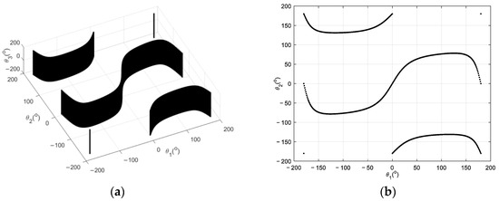
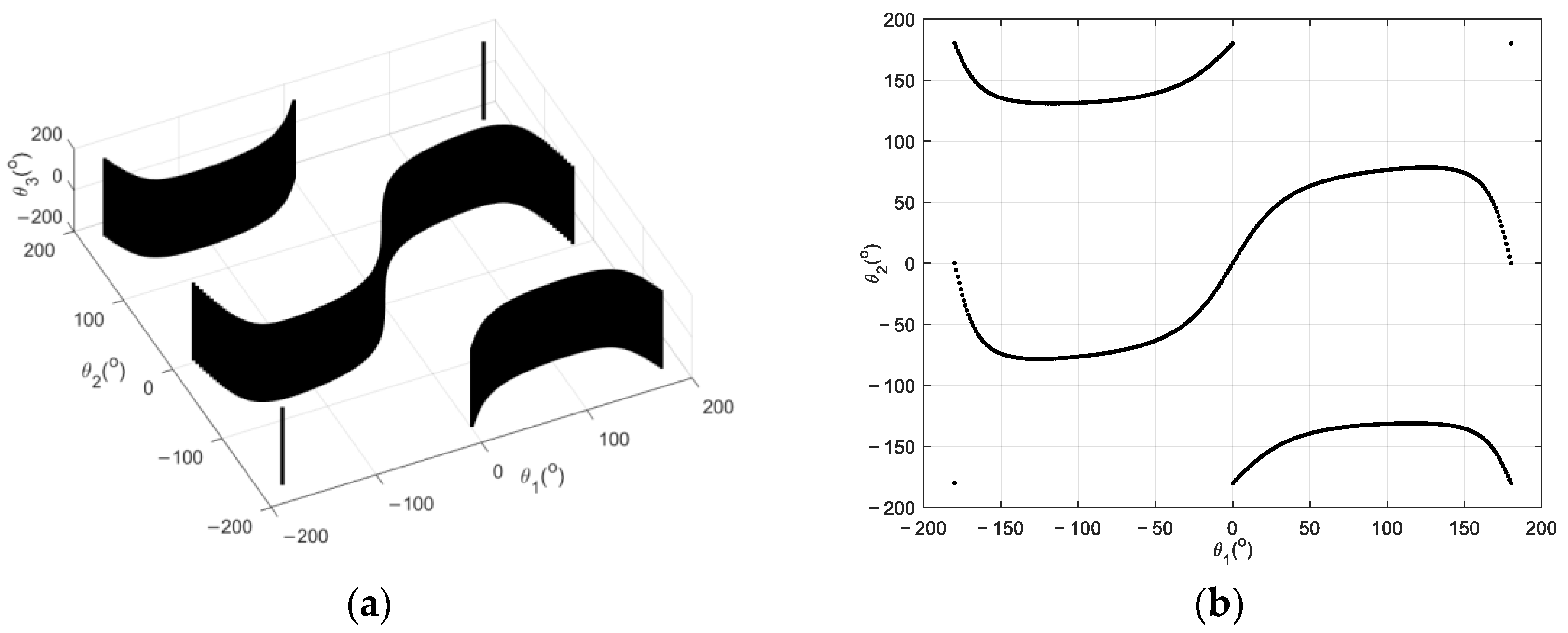
By setting the traversal step size to 2° for each dimension, the singular surface in the joint space of the planar FFSR system described in this paper is shown in Figure 2.

Figure 2. Singular surface in the joint space. (a) 3D view. (b) ${\theta }_1-{\theta }_2$ view.

As can be seen from the results in the figure above, the singular surface is symmetric about the origin in the ${\theta }_1-{\theta }_2$ plane. In fact, examining the singularity Formula (31), it follows that $M$ is an odd function of $\left({\theta }_1,{\theta }_2\right)$; i.e., $M\left({\theta }_1,{\theta }_2\right)=-M\left(-{\theta }_1,-{\theta }_2\right)$. Therefore, combining this with the previous conclusion that $M$ is independent of the joint angle ${\theta }_3$, the following properties of the singular surface for the FFSR plane can be stated:

Property 2.

Symmetry of the Singular Surface: The singular surface of the 3-DOF planar FFSR is symmetric about the origin in the  ${\theta }_1-{\theta }_2$ joint angle plane, and traverses all points in the joint angle ${\theta }_3$.

5. Path Planning for Singularity Avoidance Based on Quasi-Self-Motion

When performing path planning in the end-effector pose workspace using the resolved motion rate control, singularities may occur; therefore, how to avoid and escape from singularities is a critical issue that must be addressed in such planning algorithms. When singularity avoidance fails and the system enters a singular configuration, the problem of how to escape from the singularity arises. This chapter proposes a new solution to this problem.

5.1. Singularity Measure

The singularity measure indicates whether the system approaches or enters a singular configuration. It serves as an important criterion for performing singularity-avoidance operations during trajectory motion, and is a prerequisite for designing singularity-avoidance algorithms.

In this section, a definition of the singularity measure for the non-redundant FFSR system is given based on the determinant of the GJM, namely,

$$\kappa =\left|\det \left({\mathit{J}}_g\right)\right|,$$

(36)

In the expression, the symbol $| |$ denotes the absolute value operation. When $\kappa$ is large, the system is far from all the singular configurations; when $\kappa$ is small, it approaches a singular configuration; and when $\kappa =0$, it is completely trapped in a singularity.

5.2. Introduction to the Robust Pseudo-Inverse Method

The robust pseudo-inverse method is a commonly used algorithm for addressing singular problems. This method replaces the standard pseudo-inverse with a robust pseudo-inverse near singularities, thereby ensuring that the optimization algorithm proceeds normally in the vicinity of these points. The following is a brief introduction to this method for comparison with the method discussed in the next section.

Consider the following performance index function over the entire trajectory interval $\left[0,t_f\right]$:

$$\min J={\displaystyle \frac{1}{2}}{\displaystyle {\int }_0^{t_f}\left({\dot{\mathit{\theta }}}^T\dot{\mathit{\theta }}+{\mathit{e}}^T\mathit{R}\mathit{e}\right)dt},$$

(37)

In the above equation, $\mathit{e}\left(t\right)={\mathit{J}}_g\dot{\mathit{\theta }}\left(t\right)-{\dot{\mathit{X}}}_e\left(t\right)$ is the tracking error in the velocity of the end-effector pose, and $\mathit{R}$ is the weight matrix for this tracking error, which is a positive-definite symmetric matrix.

Solving this unconstrained optimization problem yields a robust pseudo-inverse solution for the joint angular velocity, which is:

$$\dot{\mathit{\theta }}={\mathit{J}}_g^T{\left({\mathit{J}}_g{\mathit{J}}_g^T+{\mathit{R}}^{-1}\right)}^{-1}{\dot{\mathit{X}}}_e,$$

(38)

Choose a weight matrix such that ${\mathit{R}}^{-1}=\mathit{D}=\left(\begin{array}{ccc}{\lambda }_1^2& & \\ & {\lambda }_2^2& \\ & & {\lambda }_3^2\end{array}\right)$, where ${\lambda }_i^2$ (i = 1, 2, 3) are sufficiently small non-negative scalar functions. These parameters determine the relative magnitude of the introduced velocity errors for the end-effector pose. When all the ${\lambda }_i^2$ are zero, no error is introduced into the velocity-level kinematics. The resulting robust pseudo-inverse solution is:

$$\dot{\mathit{\theta }}={\mathit{J}}_g^T{\left({\mathit{J}}_g{\mathit{J}}_g^T+\mathit{D}\right)}^{-1}{\dot{\mathit{X}}}_e,$$

(39)

Equation (39) is also commonly referred to as the damped least-squares solution, and ${\lambda }_i^2$ are called the damping factors. Considering the smoothness of the introduced errors, this paper designs the parameters ${\lambda }_i^2$ as the following half-period cosine functions adaptively adjusted based on the singularity measure:

$${\lambda }_i^2=\left\{\begin{array}{ll}0\hfill & \kappa \ge {\kappa }_0\hfill \\ {\displaystyle \frac{{\lambda }_{m,i}^2}{2}}\left(1+\cos {\displaystyle \frac{\kappa }{{\kappa }_0}}\pi \right)\hfill & \kappa <{\kappa }_0\hfill \end{array}\right.,$$

(40)

where $\kappa$ is the singularity measure at the current time, ${\kappa }_0$ is the singularity measure threshold, and ${\lambda }_{m,i}^2$ (i = 1, 2, 3) are the maximum set values of ${\lambda }_i^2$.

The robust pseudo-inverse method enables inverse kinematics calculations in singular regions, but at the cost of reduced control accuracy. Furthermore, its inability to actively move away from singularities is another significant shortcoming.

5.3. Quasi-Self-Motion Method Design

5.3.1. Analysis of the Existence of Quasi-Self-Motion

In addition to the robust pseudo-inverse method, another common technique used in engineering to avoid singularities is the self-motion method. The joint angular velocity command for self-motion, ${\dot{\mathit{\theta }}}_N$, does not produce any effective end-effector motion; that is, it satisfies:

$${\mathit{J}}_g{\dot{\mathit{\theta }}}_N=0,$$

(41)

The effect of self-motion is merely to reconfigure the joint angles of the system, thus offering the possibility of achieving singularity avoidance. Its prominent advantage is that it avoids singularities without introducing any path errors. However, in the conventional sense, self-motion configurations are typically achieved by leveraging the system’s redundant kinematic degrees of freedom, which ensures that Equation (41) has non-zero solutions. The 3-DOF planar FFSR studied in this paper does not satisfy this requirement; therefore, no conventional self-motion configuration exists.

Nevertheless, the FFSR system is subject to the angular momentum conservation constraint, which is a nonholonomic constraint. This constraint endows the motion of the end-effector pose with the following properties:

Property 3.

Path Dependence of End-Effector Pose Evolution: When the end-effector pose ${\mathit{X}}_e$ of the FFSR returns to its initial state through a closed-loop motion, the joint angles $\mathit{\theta }$ generally do not return to their initial states; the specific state depends on the motion path of ${\mathit{X}}_e$.

Proof. 

The proof is divided into three parts.

Step 1. Prove that the base attitude ${\phi }_0$ is related to the motion path of the joint angles $\mathit{\theta }$.

According to Frobenius theorem [31], a homogeneous Pfaffian constraint in n variables is denoted as:

$${\displaystyle \sum _{s=1}^n{A}_s\left(u_1,u_2,\cdots ,u_n\right)d{u}_s}=0,$$

(42)

The necessary and sufficient condition for its integrability is that the following equation holds identically:

$$A_s\left({\displaystyle \frac{\partial A_r}{u_l}}-{\displaystyle \frac{\partial A_l}{u_r}}\right)+A_r\left({\displaystyle \frac{\partial A_l}{u_s}}-{\displaystyle \frac{\partial A_s}{u_l}}\right)+A_l\left({\displaystyle \frac{\partial A_s}{u_r}}-{\displaystyle \frac{\partial A_r}{u_s}}\right)=0, s,r,l=1,2,\cdots ,n,$$

(43)

For the FFSR system, examining the angular momentum conservation constraint (10), it is evident that this constraint is of the Pfaffian form:

$$A_1=I_{\omega }, A_2=I_{\theta 1}, A_3=I_{\theta 2}, A_4=I_{\theta 3},$$

(44)

Take $s=2$, $r=3$, $l=4$ to verify condition (43): arbitrarily select a state point ${\left(\begin{array}{cc}{\phi }_0& {\mathit{\theta }}^T\end{array}\right)}^T$ and compute the left-hand side of (43). The result is generally nonzero, meaning that the necessary and sufficient condition for integrability does not hold identically; therefore, (10) is non-integrable. Furthermore, from (10) it follows that the base attitude ${\phi }_0$ is obtained by the path integral of $\mathit{\theta }$:

$${\phi }_0={\displaystyle {\int }_{L\left(\mathit{\theta }\right)}\left(-\frac{{\mathit{I}}_{\theta }}{I_{\omega }}\left(\mathit{\theta }\right)\right)d\mathit{\theta }},$$

(45)

From Stokes’ theorem and the necessary and sufficient conditions for the path-independence of spatial line integrals, it follows that if the integral of ${\phi }_0$ is independent of the path of $\mathit{\theta }$, then Equation (10) would be integrable, which contradicts the conclusion that it is non-integrable. Therefore, ${\phi }_0$ depends on the path of $\mathit{\theta }$.

Step 2. Prove that when $\mathit{\theta }$ undergoes a closed-loop motion, ${\mathit{X}}_e$ does not return to its initial state.

When $\mathit{\theta }$ performs a closed-loop motion, take two points of $\mathit{\theta }$: the starting point ${\mathit{\theta }}^{\left(1\right)}$ and an arbitrary intermediate point ${\mathit{\theta }}^{\left(2\right)}$, dividing the closed loop into two different paths $L_1$ and $L_2$. If ${\phi }_0$ returns to its initial state, then its integral along $L_1+L_2$ is zero. Note that for line integrals with respect to coordinate variables, the integral along an arbitrary curve $L_2$ equals the negative of the integral along its reverse curve $-L_2$. This is because, after reversing the curve, the integrand remains unchanged, while the integration limits of the corresponding definite integral become reversed. According to the rules of definite integration, it readily follows that the resulting integral is the negative of the original result. Such result implies that the integrals along $L_1$ and $-L_2$ are equal. However, $L_1$ and $-L_2$ are two arbitrary different paths connecting ${\mathit{\theta }}^{\left(1\right)}$ to an arbitrary point ${\mathit{\theta }}^{\left(2\right)}$, indicating that the integral result is path-independent, which contradicts the conclusion obtained in the previous step. Therefore, under a closed-loop motion of $\mathit{\theta }$, the base attitude ${\phi }_0$ does not return to the initial state. Finally, according to Equations (5) and (7), the end-effector pose ${\mathit{X}}_e$ is an algebraic function of the current values of ${\phi }_0$ and $\mathit{\theta }$, and thus ${\mathit{X}}_e$, like ${\phi }_0$, does not return to the initial state.

Then, based on the conclusion reached in the previous step, the equivalence of the contrapositive implies that when the end-effector pose ${\mathit{X}}_e$ undergoes a closed-loop motion, the joint angles $\mathit{\theta }$ do not return to its initial state.

Step 3. Prove that when the end-effector pose ${\mathit{X}}_e$ undergoes a closed-loop motion, the final state of the joint angles $\mathit{\theta }$ is related to the motion path of ${\mathit{X}}_e$ rather than being a unique value. If this conclusion were false, the end-effector pose ${\mathit{X}}_e$ and the joint angles $\mathit{\theta }$ would have a one-to-one mapping relationship. However, based on the modeling results in Chapter 2, we know that ${\mathit{X}}_e$ is an algebraic function of the base attitude ${\phi }_0$ and the joint angles $\mathit{\theta }$. Since it has already proved in Step 1 that ${\phi }_0$ is related to the motion path of $\mathit{\theta }$, it follows that ${\mathit{X}}_e$ is also related to the motion path of $\mathit{\theta }$ and does not have a one-to-one mapping. The proof by contradiction shows that the conclusion holds.□

According to Property 3, a closed-loop motion of the end-effector pose ${\mathit{X}}_e$ is a way to adjust the joint angles $\mathit{\theta }$ while keeping its own state at the end of the motion unchanged. On the other hand, Property 1 indicates that the system’s singular configurations depend solely on the current joint angles. Therefore, using the closed-loop motion of ${\mathit{X}}_e$ to reconfigure $\mathit{\theta }$ is a possible way for the system to avoid singularities. We refer to this closed-loop motion of the end-effector pose as quasi-self-motion.

5.3.2. Quasi-Self-Motion Method Design for Singularity Avoidance

This section first derives a basic module for quasi-self-motion design, and then, based on this, designs a singularity-avoidance method for the system. The objective of this module is: Given the end-effector pose ${\mathit{X}}_e$, find a joint angle configuration ${\mathit{\theta }}^{*}$ that maximizes the system singularity measure ${\kappa }^{*}$. The derivation of the module is as follows.

First, a kinematically equivalent virtual manipulator (VM) model is introduced for the FFSRs [32]. Define the virtual link vectors:

$${\widehat{\mathit{a}}}_j={\displaystyle \frac{1}{M}}\left({\displaystyle \sum _{i=0}^{j-1}{m}_i}\right){\mathit{a}}_j, j=1,\cdots ,3,$$

(46)

$${\widehat{\mathit{b}}}_j={\displaystyle \frac{1}{M}}\left({\displaystyle \sum _{i=0}^j{m}_i}\right){\mathit{b}}_j, j=0,\cdots ,3,$$

(47)

The position-level kinematic equations for the end-effector pose based on the virtual links can be expressed as:

$${\phi }_e={\phi }_0+{\displaystyle \sum _{i=1}^3{\theta }_i},$$

(48)

$${\mathit{r}}_e={\mathit{r}}_g+{\widehat{\mathit{b}}}_0+{\displaystyle \sum _{i=1}^3\left({\widehat{\mathit{a}}}_i+{\widehat{\mathit{b}}}_i\right)},$$

(49)

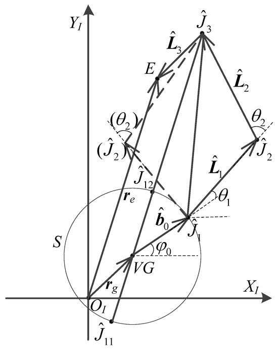
The kinematic equations for the end-effector pose, as expressed in Equations (48) and (49), bear a strong formal resemblance to those of a fixed-base manipulator. Consequently, an equivalent fixed-base robot model, referred to as the VM model, can be constructed, as shown in Figure 3. The system’s center of mass is the virtual ground (VG), which serves as the fixed base of the VM model; the virtual link vectors defined by Equations (46) and (47) align with the directions of the corresponding original links and are proportional in length.

Figure 3. Schematic diagram of the VM model for the 3-DOF Planar FFSR.

Define the length of the virtual link:

$${\widehat{L}}_j=\left|{\widehat{\mathit{a}}}_j+{\widehat{\mathit{b}}}_j\right|={\displaystyle \frac{1}{M}}\left|\left({\displaystyle \sum _{i=0}^{j-1}{m}_i}\right)c_{j,1}+\left({\displaystyle \sum _{i=0}^j{m}_i}\right)c_{j,2}\right|L_j, j=1,2,3,$$

(50)

and virtual link vectors:

$${\widehat{\mathit{L}}}_j={\widehat{\mathit{a}}}_j+{\widehat{\mathit{b}}}_j={\widehat{L}}_j{\left(\begin{array}{cc}\cos \left({\phi }_0+{\displaystyle \sum _{i=1}^j{\theta }_i}\right)& \sin \left({\phi }_0+{\displaystyle \sum _{i=1}^j{\theta }_i}\right)\end{array}\right)}^T, j=1,2,3,$$

(51)

Substituting Equation (51) into Equation (49) yields:

$${\mathit{r}}_e={\mathit{r}}_g+{\widehat{\mathit{b}}}_0+{\displaystyle \sum _{i=1}^3{\widehat{\mathit{L}}}_i},$$

(52)

We derive the algorithm using geometric methods. The geometric relationships among the quantities in Equation (52) are shown in Figure 4.

Figure 4. Geometric diagram of position-level kinematics in the inertial frame.

In the figure, circle $S$ represents the set of all possible positions that the end point ${\widehat{J}}_1$ of the virtual link vector ${\widehat{\mathit{b}}}_0$ can reach depending on the base attitude ${\phi }_0$. $E$ is the given end point of the manipulator, whose pose is ${\mathit{X}}_e$. Since both ${\mathit{X}}_e$ and ${\widehat{L}}_3$ are fixed, it follows that the pose of vector ${\widehat{\mathit{L}}}_3={\widehat{L}}_3{\left(\begin{array}{cc}\cos {\phi }_e& \sin {\phi }_e\end{array}\right)}^T$ is fixed. A line connecting the starting point ${\widehat{J}}_3$ of ${\widehat{\mathit{L}}}_3$ and the virtual ground VG intersects circle $S$ at two points ${\widehat{J}}_{11}$ and ${\widehat{J}}_{12}$, respectively.

Suppose that the connection point ${\widehat{J}}_2$ of ${\widehat{\mathit{L}}}_1$ and ${\widehat{\mathit{L}}}_2$ lies to the right of ${\widehat{J}}_1{\widehat{J}}_3$. Then, in $\Delta {\widehat{J}}_1{\widehat{J}}_2{\widehat{J}}_3$, by the law of cosines, we have:

$${\left|{\widehat{J}}_1{\widehat{J}}_3\right|}^2={\left|{\widehat{J}}_1{\widehat{J}}_2\right|}^2+{\left|{\widehat{J}}_2{\widehat{J}}_3\right|}^2-2\left|{\widehat{J}}_1{\widehat{J}}_2\right|\left|{\widehat{J}}_2{\widehat{J}}_3\right|\cos \left(180°-{\theta }_2\right),$$

(53)

where

$$\left|{\widehat{J}}_1{\widehat{J}}_3\right|=\left|{\mathit{r}}_e-{\widehat{\mathit{L}}}_3-{\mathit{r}}_g-{\widehat{\mathit{b}}}_0\right|,$$

(54)

$$\left|{\widehat{J}}_1{\widehat{J}}_2\right|={\widehat{L}}_1,$$

(55)

$$\left|{\widehat{J}}_2{\widehat{J}}_3\right|={\widehat{L}}_2,$$

(56)

Note also that when ${\widehat{J}}_2$ is to the right of ${\widehat{J}}_1{\widehat{J}}_3$, ${\theta }_2\in \left[0,180°\right]$. From Equations (53)–(56), we obtain:

$${\theta }_2=180°-\mathrm{acos}\left({\displaystyle \frac{{\widehat{L}}_1^2+{\widehat{L}}_2^2-{\left|{\mathit{r}}_e-{\widehat{\mathit{L}}}_3-{\mathit{r}}_g-{\widehat{\mathit{b}}}_0\right|}^2}{2{\widehat{L}}_1{\widehat{L}}_2}}\right),$$

(57)

Calculate the coordinates of ${\widehat{J}}_1$ and ${\widehat{J}}_3$, which are:

$${\widehat{\mathit{J}}}_1={\left(\begin{array}{cc}{\widehat{J}}_{1x}& {\widehat{J}}_{1y}\end{array}\right)}^T={\mathit{r}}_g+{\widehat{\mathit{b}}}_0,$$

(58)

$${\widehat{\mathit{J}}}_3={\left(\begin{array}{cc}{\widehat{J}}_{3x}& {\widehat{J}}_{3y}\end{array}\right)}^T={\mathit{r}}_e-{\widehat{\mathit{L}}}_3={\mathit{r}}_e-{\widehat{L}}_3{\left(\begin{array}{cc}\cos {\phi }_e& \sin {\phi }_e\end{array}\right)}^T,$$

(59)

Based on the vector relationship:

$$\overrightarrow{{\widehat{J}}_1{\widehat{J}}_3}={\widehat{\mathit{J}}}_3-{\widehat{\mathit{J}}}_1={\widehat{\mathit{L}}}_1+{\widehat{\mathit{L}}}_2,$$

(60)

we have:

$${\widehat{L}}_1\left(\begin{array}{c}\cos \left({\phi }_0+{\theta }_1\right)\\ \sin \left({\phi }_0+{\theta }_1\right)\end{array}\right)+{\widehat{L}}_2\left(\begin{array}{c}\cos \left({\phi }_0+{\theta }_1+{\theta }_2\right)\\ \sin \left({\phi }_0+{\theta }_1+{\theta }_2\right)\end{array}\right)={\widehat{\mathit{J}}}_3-{\widehat{\mathit{J}}}_1,$$

(61)

Substituting Equations (58) and (59) into Equation (61) and then expanding yields:

$$\left(\begin{array}{cc}{\widehat{L}}_1+{\widehat{L}}_2\cos {\theta }_2& -{\widehat{L}}_2\sin {\theta }_2\\ {\widehat{L}}_1+{\widehat{L}}_2\cos {\theta }_2& {\widehat{L}}_2\sin {\theta }_2\end{array}\right)\left(\begin{array}{c}\cos x\\ \sin x\end{array}\right)=\left(\begin{array}{c}{\widehat{J}}_{3x}-{\widehat{J}}_{1x}\\ {\widehat{J}}_{3y}-{\widehat{J}}_{1y}\end{array}\right), x={\phi }_0+{\theta }_1,$$

(62)

Let:

$$\left\{\begin{array}{l}{p}_1={\widehat{L}}_1+{\widehat{L}}_2\cos {\theta }_2\hfill \\ p_2={\widehat{L}}_2\sin {\theta }_2\hfill \end{array}\right.,$$

(63)

From Equation (62), we obtain:

$$\left(\begin{array}{c}\cos x\\ \sin x\end{array}\right)={\displaystyle \frac{1}{p_1^2+p_2^2}}\left(\begin{array}{cc}{p}_1& p_2\\ -p_2& p_1\end{array}\right)\left(\begin{array}{c}{\widehat{J}}_{3x}-{\widehat{J}}_{1x}\\ {\widehat{J}}_{3y}-{\widehat{J}}_{1y}\end{array}\right)={\displaystyle \frac{1}{p_1^2+p_2^2}}\left(\begin{array}{c}{p}_1\left({\widehat{J}}_{3x}-{\widehat{J}}_{1x}\right)+p_2\left({\widehat{J}}_{3y}-{\widehat{J}}_{1y}\right)\\ -p_2\left({\widehat{J}}_{3x}-{\widehat{J}}_{1x}\right)+p_1\left({\widehat{J}}_{3y}-{\widehat{J}}_{1y}\right)\end{array}\right),$$

(64)

This leads to:

$$x=\mathrm{atan} 2\left(-p_2\left({\widehat{J}}_{3x}-{\widehat{J}}_{1x}\right)+p_1\left({\widehat{J}}_{3y}-{\widehat{J}}_{1y}\right),p_1\left({\widehat{J}}_{3x}-{\widehat{J}}_{1x}\right)+p_2\left({\widehat{J}}_{3y}-{\widehat{J}}_{1y}\right)\right),$$

(65)

and

$${\theta }_1=\mathrm{atan} 2\left(-p_2\left({\widehat{J}}_{3x}-{\widehat{J}}_{1x}\right)+p_1\left({\widehat{J}}_{3y}-{\widehat{J}}_{1y}\right),p_1\left({\widehat{J}}_{3x}-{\widehat{J}}_{1x}\right)+p_2\left({\widehat{J}}_{3y}-{\widehat{J}}_{1y}\right)\right)-{\phi }_0,$$

(66)

Finally, from Equation (48) we have:

$${\theta }_3={\phi }_e-{\phi }_0-{\theta }_1-{\theta }_2,$$

(67)

Substituting Equations (57) and (66) into the above equation yields ${\theta }_3$. Combining Equations (57), (66) and (67) gives the desired joint angles $\mathit{\theta }={\left(\begin{array}{ccc}{\theta }_1& {\theta }_2& {\theta }_3\end{array}\right)}^T$.

When point ${\widehat{J}}_2$ lies to the left of ${\widehat{J}}_1{\widehat{J}}_3$, ${\theta }_2\in \left[-180°,0\right]$. In $\Delta {\widehat{J}}_1{\widehat{J}}_2{\widehat{J}}_3$, by the law of cosines, we have:

$${\left|{\widehat{J}}_1{\widehat{J}}_3\right|}^2={\left|{\widehat{J}}_1{\widehat{J}}_2\right|}^2+{\left|{\widehat{J}}_2{\widehat{J}}_3\right|}^2-2\left|{\widehat{J}}_1{\widehat{J}}_2\right|\left|{\widehat{J}}_2{\widehat{J}}_3\right|\cos \left(180°+{\theta }_2\right),$$

(68)

and thus we obtain:

$${\theta }_2=\mathrm{acos}\left({\displaystyle \frac{{\widehat{L}}_1^2+{\widehat{L}}_2^2-{\left|{\mathit{r}}_e-{\widehat{\mathit{L}}}_3-{\mathit{r}}_g-{\widehat{\mathit{b}}}_0\right|}^2}{2{\widehat{L}}_1{\widehat{L}}_2}}\right)-180°,$$

(69)

The other steps are the same as when point ${\widehat{J}}_2$ is located to the right of ${\widehat{J}}_1{\widehat{J}}_3$.

At this point, under the premise that the end-effector pose ${\mathit{X}}_e$ is fixed, the joint angles $\mathit{\theta }\left({\phi }_0\right)$ corresponding to a specified base attitude ${\phi }_0$ has been obtained. Furthermore, according to the joint closed-loop self-correction method [32], if the reachability of the end-effector pose is disregarded, all attitudes within its domain $\left[-180°,180°\right)$ can be achieved under closed-loop self-correction motion. Therefore, from the above derivation, when ${\mathit{X}}_e$ is fixed, the function of the joint angles $\mathit{\theta }=\mathit{\theta }\left({\phi }_0\right)$ with respect to all base attitudes ${\phi }_0\in \left[-180°,180°\right)$ can be obtained. Combined with the singularity measure definition (36), the function of the system singularity measure with respect to the base attitude is expressed as:

$$\kappa =\left|\det \left({\mathit{J}}_g\left(\mathit{\theta }\left({\phi }_0\right)\right)\right)\right|=\kappa \left({\phi }_0\right),$$

(70)

Therefore, it suffices to find the maximum value ${\kappa }^{*}$ of the singularity measure within the range ${\phi }_0\in \left[-180°,180°\right)$. In this paper, the domain of the decision variable ${\phi }_0$ is discretized into a grid, and a local maximum is computed within each grid cell. A finer grid yields higher accuracy for the local extrema but incurs greater computational cost. To balance computational expense and extremum accuracy, the recommended grid step size for ${\phi }_0$ ranges from 0.1 deg to 2.0 deg. Alternatively, one may first perform a coarse search with a larger step size within this range, and then conduct a finer search with a smaller step size within the extremum intervals identified by the coarse search. Through comprehensive comparison, the global maximum of the singularity measure is ultimately obtained. The module derivation is now complete.

Based onthe module above, during the path planning process using the resolved motion rate control method according to Equation (20), singularity avoidance for the FFSR based on quasi-self-motion can be achieved. The specific steps are as follows:

• Set a singularity measure threshold ${\kappa }_0$. In each planning step calculation, first evaluate the singularity measure $\kappa \left(t_c\right)$ at the current time $t_c$. If $\kappa \left(t_c\right)<{\kappa }_0$, it indicates that the system is approaching singularity; then pause the tracking motion of the desired path and proceed to the next step. Otherwise, the system is non-singular, and path planning can be performed using resolved motion rate control.
• Use the module to determine the maximum singularity measure ${\kappa }^{*}\left(t_c\right)$ for the current end-effector pose ${\mathit{X}}_e\left(t_c\right)$, along with the corresponding base attitude ${\phi }_0^{*}\left(t_c\right)$ and joint angles ${\mathit{\theta }}^{*}\left(t_c\right)$. Then, taking ${\mathit{q}}^{*}={\left(\begin{array}{cc}{\phi }_0^{*}& {\left({\mathit{\theta }}^{*}\right)}^T\end{array}\right)}^T$ as the desired state, use the Basis Algorithm [33] to reconfigure the system state to the desired state ${\mathit{q}}^{*}$.
• After reconfiguration is completed, the system arrives at a new time $t_{c1}$ and is now in a state ${\mathit{q}}^{*}\left(t_{c1}\right)$ far from singularity; at this point, resume tracking of the desired path using resolved motion rate control.

It can be seen that the quasi-self-motion method inserts a reconfiguration motion segment $\kappa \left(t_c\right)\to {\kappa }^{*}\left(t_{c1}\right)$ at the singular state $\kappa \left(t_c\right)$, which increases the total duration of the path planning and, consequently, alters the terminal time $t_f$ of the trajectory motion. Therefore, the method is applicable to scenarios where the target end-effector pose ${\mathit{X}}_e$ remains constant throughout the mission (i.e., aside from the spatial robot motion caused by the robotic arm’s movements, there is no other relative motion of the target pose with respect to the spatial robot). In on-orbit servicing missions, path planning can be categorized into cooperative-target path planning and non-cooperative-target path planning based on the cooperation status of the target [34]. When the target is cooperative, the desired target pose is generally fixed, allowing brief pauses to be inserted during the trajectory motion. Such missions primarily include on-orbit assembly and maintenance, on-orbit refueling, etc. Studies such as [25,29,34,35] have conducted path planning in this context, and the method proposed in this paper is also mainly applicable to this scenario. When the target is non-cooperative, such as in space debris capture missions, the target pose is in an unfixed or even unpredictable state of change, for which the proposed method is not currently applicable.

5.3.3. Calculation of End-Effector Pose Space Without Quasi-Self-Motion

Quasi-self-motion exists because the mapping point $\mathit{\theta }$ in the joint space for a given end-effector pose ${\mathit{X}}_e$ is not unique; when there is only a unique mapping for the current state, quasi-self-motion does not exist.

When the mapping from the end-effector pose ${\mathit{X}}_e$ to the joint angles $\mathit{\theta }$ is unique, it means that the mapping from ${\mathit{X}}_e$ to the base attitude ${\phi }_0$ is unique. Next, we examine the range of values for ${\phi }_0$. Figure 4 shows that the range of values for ${\phi }_0$ is determined by the motion range of point ${\widehat{J}}_1$. Denote point VG as $C$. In $\Delta {\widehat{J}}_{1}C{\widehat{J}}_3$, according to the law of cosines, the length of ${\widehat{J}}_1{\widehat{J}}_3$ can be written as

$$\left|{\widehat{J}}_1{\widehat{J}}_3\right|=\sqrt{{\left|{\widehat{J}}_{1}C\right|}^2+{\left|{\widehat{J}}_{3}C\right|}^2-2\left|{\widehat{J}}_{1}C\right|\left|{\widehat{J}}_{3}C\right|\cos \angle {\widehat{J}}_{1}C{\widehat{J}}_3},$$

(71)

In the equation above, $\left|{\widehat{J}}_{1}C\right|=\left|{\mathit{r}}_e-{\mathit{r}}_g\right|$ and $\left|{\widehat{J}}_{3}C\right|=\left|{\mathit{b}}_0\right|$ are both constant values.

Consider the motion of point ${\widehat{J}}_1$ along the right arc of circle $S$. As ${\widehat{J}}_1$ slides gradually from the highest point ${\widehat{J}}_{12}$ to the lowest point ${\widehat{J}}_{11}$ on the arc, $\angle {\widehat{J}}_{1}C{\widehat{J}}_3$ increases monotonically from 0 to 180°. Furthermore, from Equation (71), it can be seen that $\left|{\widehat{J}}_1{\widehat{J}}_3\right|$ is monotonically increasing with respect to $\angle {\widehat{J}}_{1}C{\widehat{J}}_3$ when $\angle {\widehat{J}}_{1}E{\widehat{J}}_3\in \left[0,180°\right]$, and its range is:

$$\left|{\widehat{J}}_3{\widehat{J}}_{12}\right|\le \left|{\widehat{J}}_1{\widehat{J}}_3\right|\le \left|{\widehat{J}}_3{\widehat{J}}_{11}\right|,$$

(72)

On the other hand, based on the vector relationship, the possible range of values for $\left|{\widehat{J}}_1{\widehat{J}}_3\right|$ is

$$\left|{\widehat{L}}_1-{\widehat{L}}_2\right|\le \left|{\widehat{J}}_1{\widehat{J}}_3\right|=\left|{\widehat{\mathit{L}}}_1+{\widehat{\mathit{L}}}_2\right|\le {\widehat{L}}_1+{\widehat{L}}_2,$$

(73)

This leads to the following:

• When

$${\widehat{L}}_1+{\widehat{L}}_2>\left|{\widehat{L}}_1-{\widehat{L}}_2\right|\ge \left|{\widehat{J}}_3{\widehat{J}}_{12}\right|,$$

(74)

denote the solution of the equation:

$$\left|{\widehat{J}}_1{\widehat{J}}_3\right|=\sqrt{{\left|{\widehat{J}}_{1}C\right|}^2+{\left|{\widehat{J}}_{3}C\right|}^2-2\left|{\widehat{J}}_{1}C\right|\left|{\widehat{J}}_{3}C\right|\cos \angle {\widehat{J}}_{1}C{\widehat{J}}_3}=\left|{\widehat{L}}_1-{\widehat{L}}_2\right|,$$

(75)

with respect to ${\widehat{J}}_1$ as point ${\widehat{J}}_{13}$, and the solution of equation:

$$\left|{\widehat{J}}_1{\widehat{J}}_3\right|=\sqrt{{\left|{\widehat{J}}_{1}C\right|}^2+{\left|{\widehat{J}}_{3}C\right|}^2-2\left|{\widehat{J}}_{1}C\right|\left|{\widehat{J}}_{3}C\right|\cos \angle {\widehat{J}}_{1}C{\widehat{J}}_3}={\widehat{L}}_1+{\widehat{L}}_2,$$

(76)

with respect to ${\widehat{J}}_1$ as point ${\widehat{J}}_{14}$. Then the range of values on the right side of circle $S$ where ${\widehat{J}}_1$ has non-unique solutions is ${\widehat{J}}_1\in \stackrel{⏜}{{\widehat{J}}_{13}{\widehat{J}}_{14}}$, and it is not difficult to infer that on the left side of circle $S$ there exists another half-range of non-unique solutions, symmetric to $\stackrel{⏜}{{\widehat{J}}_{13}{\widehat{J}}_{14}}$ about axis ${\widehat{J}}_{11}{\widehat{J}}_{12}$, denoted as $\stackrel{⏜}{{\widehat{J}}_{15}{\widehat{J}}_{16}}$. That is, the entire range of ${\widehat{J}}_1$ is ${\widehat{J}}_1\in \stackrel{⏜}{{\widehat{J}}_{13}{\widehat{J}}_{14}}\cup \stackrel{⏜}{{\widehat{J}}_{15}{\widehat{J}}_{16}}$.

• When

$${\widehat{L}}_1+{\widehat{L}}_2<\left|{\widehat{J}}_3{\widehat{J}}_{12}\right|,$$

(77)

there is no solution for point ${\widehat{J}}_1$, meaning that the end-effector pose ${\mathit{X}}_e$ cannot be reached at this time.

• When

$${\widehat{L}}_1+{\widehat{L}}_2=\left|{\widehat{J}}_3{\widehat{J}}_{12}\right|,$$

(78)

point ${\widehat{J}}_1$ has a unique solution ${\widehat{J}}_1={\widehat{J}}_{12}$.

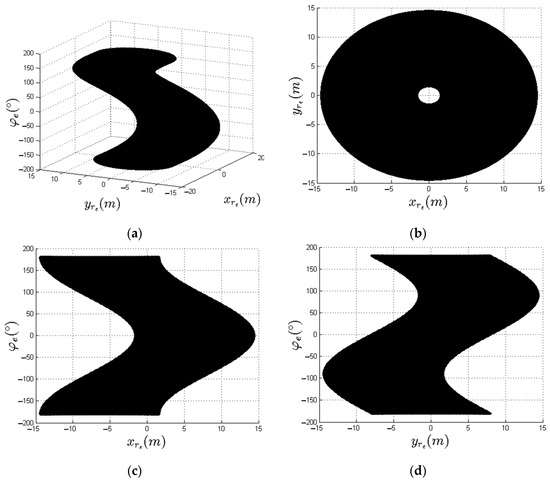
Therefore, the necessary and sufficient condition for the absence of quasi-self-motion in the end-effector pose is that ${\mathit{X}}_e$ satisfies Equation (78). Equation (78) can be expanded as:

$${\widehat{L}}_1+{\widehat{L}}_2=\left|{\widehat{J}}_3{\widehat{J}}_{12}\right|=\left|\left|{\widehat{J}}_{3}C\right|-\left|{\widehat{J}}_{12}C\right|\right|=\left|\left|{\mathit{r}}_e-{\widehat{\mathit{L}}}_3-{\mathit{r}}_g\right|-\left|{\widehat{\mathit{b}}}_0\right|\right|,$$

(79)

that is,

$$\left|{\mathit{r}}_e-{\widehat{\mathit{L}}}_3-{\mathit{r}}_g\right|=\left|{\widehat{\mathit{b}}}_0\right|\pm \left({\widehat{L}}_1+{\widehat{L}}_2\right),$$

(80)

In the model with the parameters shown in Table 1 of this paper, $\left|{\widehat{\mathit{b}}}_0\right|-\left({\widehat{L}}_1+{\widehat{L}}_2\right)<0$, so the above equation has a solution only when the sign is positive. Let the components of the relevant vectors be denoted as:

$${\mathit{X}}_{\mathrm{e}}={\left(\begin{array}{cc}{\phi }_{\mathrm{e}}& {\mathit{r}}_{\mathrm{e}}^T\end{array}\right)}^T={\left(\begin{array}{ccc}{\phi }_{\mathrm{e}}& x_{r_e}& y_{r_e}\end{array}\right)}^T,$$

(81)

$${\mathit{r}}_{\mathrm{g}}={\left(\begin{array}{cc}{x}_{r_g}& y_{r_g}\end{array}\right)}^T,$$

(82)

$${\widehat{b}}_0=\left|{\widehat{\mathit{b}}}_0\right|,$$

(83)

Substituting into Equation (80), the necessary and sufficient condition for the absence of quasi-self-motion in ${\mathit{X}}_e$ is that its components satisfy the following equation:

$${\left(x_{r_e}-{\widehat{L}}_3\cos {\phi }_{\mathrm{e}}-x_{r_g}\right)}^2+{\left(y_{r_e}-{\widehat{L}}_3\sin {\phi }_{\mathrm{e}}-y_{r_g}\right)}^2={\left({\widehat{b}}_0+{\widehat{L}}_1+{\widehat{L}}_2\right)}^2,$$

(84)

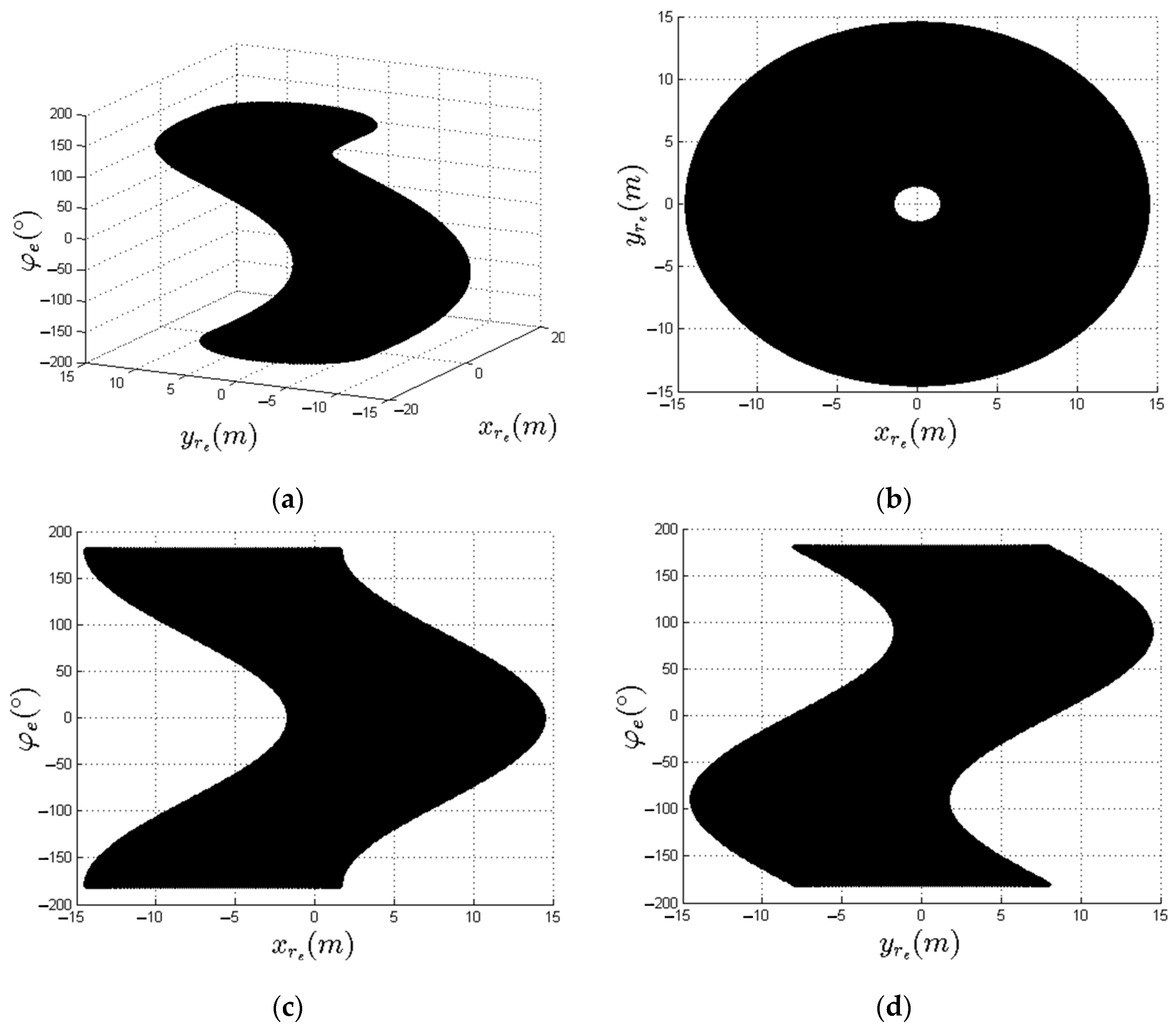
Based on the model parameters shown in Table 1, the regions in the entire end-effector pose workspace where quasi-self-motion does not exist are plotted according to Equation (84), as shown in Figure 5.

Figure 5. End-effector pose space without quasi-self-motion. (a) 3D view. (b) $x_{r_e}-y_{r_e}$ view. (c) $x_{r_e}-{\phi }_e$ view. (d) $y_{r_e}-{\phi }_e$ view.

6. Numerical Simulations

In this chapter, simulations are conducted for the quasi-self-motion-based singularity-avoidance path planning.

Set the origin of the inertial coordinate system ${\Sigma }_I$ to the system’s center of mass. Let the initial time be 0; the initial state of the FFSR is: base attitude ${\phi }_0\left(t_0\right)=18.0°$, joint angles $\mathit{\theta }\left(t_0\right)={\left(\begin{array}{ccc}-35.0°& 27.0°& -5.0°\end{array}\right)}^T$. From this, the initial end-effector pose are ${\mathit{X}}_{\mathrm{e}}\left(t_0\right)=\left(\begin{array}{c}{\phi }_{\mathrm{e}}\left(t_0\right)\\ x_{r_e}\left(t_0\right)\\ y_{r_e}\left(t_0\right)\end{array}\right)=\left(\begin{array}{c}5.0°\\ 14.151 \mathrm{m}\\ 0.513 \mathrm{m}\end{array}\right)$.

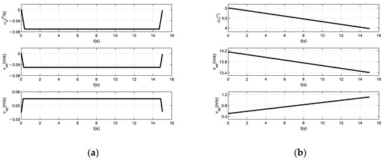
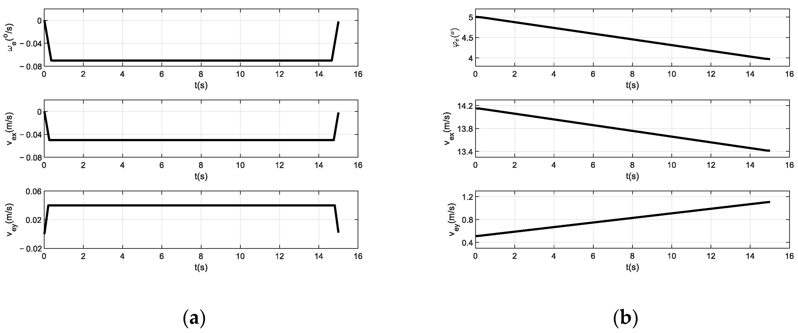
Set the end-effector pose to move for 15 s along the following trapezoidal velocity profile. The expressions for the trapezoidal velocity ${\dot{\mathit{X}}}_{\mathrm{e}}\left(t\right)=\left(\begin{array}{c}{\omega }_{\mathrm{e}}\left(t\right)\\ {\mathit{v}}_{\mathrm{e}}\left(t\right)\end{array}\right)=\left(\begin{array}{c}{\omega }_{\mathrm{e}}\left(t\right)\\ v_{\mathrm{e}\mathrm{x}}\left(t\right)\\ v_{\mathrm{e}\mathrm{x}}\left(t\right)\end{array}\right)$ are given in Equations (85)–(87); the velocity curve is shown in Figure 6a. The expressions for the corresponding displacement ${\mathit{X}}_{\mathrm{e}}\left(t\right)=\left(\begin{array}{c}{\phi }_{\mathrm{e}}\left(t\right)\\ {\mathit{r}}_{\mathrm{e}}\left(t\right)\end{array}\right)=\left(\begin{array}{c}{\phi }_{\mathrm{e}}\left(t\right)\\ r_{\mathrm{e}\mathrm{x}}\left(t\right)\\ r_{\mathrm{e}\mathrm{x}}\left(t\right)\end{array}\right)$ are given in Equations (88)–(90); the displacement curve is shown in Figure 6b.

$${\omega }_{\mathrm{e}}\left(t\right)=\left\{\begin{array}{ll}-0.2t\hfill & \hfill 0.0\le t<0.35\\ -0.07\hfill & \hfill 0.35\le t<14.65\\ -0.07+0.2\left(t-14.65\right)\hfill & \hfill 14.65\le t\le 15.0\end{array}\right.,$$

(85)

$$v_{ex}\left(t\right)=\left\{\begin{array}{ll}-0.2t\hfill & \hfill 0.0\le t<0.25\\ -0.05\hfill & \hfill 0.25\le t<14.75\\ -0.05+0.2\left(t-14.75\right)\hfill & \hfill 14.75\le t\le 15.0\end{array}\right.,$$

(86)

$$v_{ey}\left(t\right)=\left\{\begin{array}{ll}0.2t\hfill & \hfill 0.0\le t<0.20\\ 0.05\hfill & \hfill 0.20\le t<14.80\\ 0.05-0.2\left(t-14.80\right)\hfill & \hfill 14.80\le t\le 15.0\end{array}\right.,$$

(87)

$${\phi }_{\mathrm{e}}\left(t\right)=\left\{\begin{array}{ll}5.0-0.1t^2\hfill & \hfill 0.0\le t<0.35\\ 4.988-0.07\left(t-0.35\right)\hfill & \hfill 0.35\le t<14.65\\ 3.987-0.07\left(t-14.65\right)+0.1{\left(t-14.65\right)}^2\hfill & \hfill 14.65\le t\le 15.0\end{array}\right.,$$

(88)

$$r_{ex}\left(t\right)=\left\{\begin{array}{ll}14.151-0.1t^2\hfill & \hfill 0.0\le t<0.25\\ 14.145-0.05\left(t-0.25\right)\hfill & \hfill 0.25\le t<14.75\\ 13.420-0.05\left(t-14.75\right)+0.1{\left(t-14.75\right)}^2\hfill & \hfill 14.75\le t\le 15.0\end{array}\right.,$$

(89)

$$r_{ey}\left(t\right)=\left\{\begin{array}{ll}0.513+0.1t^2\hfill & \hfill 0.0\le t<0.20\\ 0.517+0.04\left(t-14.80\right)\hfill & \hfill 0.20\le t<14.80\\ 1.101+0.042\left(t-14.80\right)-0.1{\left(t-14.80\right)}^2\hfill & \hfill 14.80\le t\le 15.0\end{array}\right.,$$

(90)

Figure 6. Desired (a) velocity and (b) displacement curve for the end-effector pose.

This chapter presents simulation examples of path planning for the joint angles of the FFSR using resolved motion rate control, employing different methods for singularity avoidance.

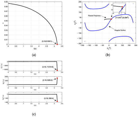
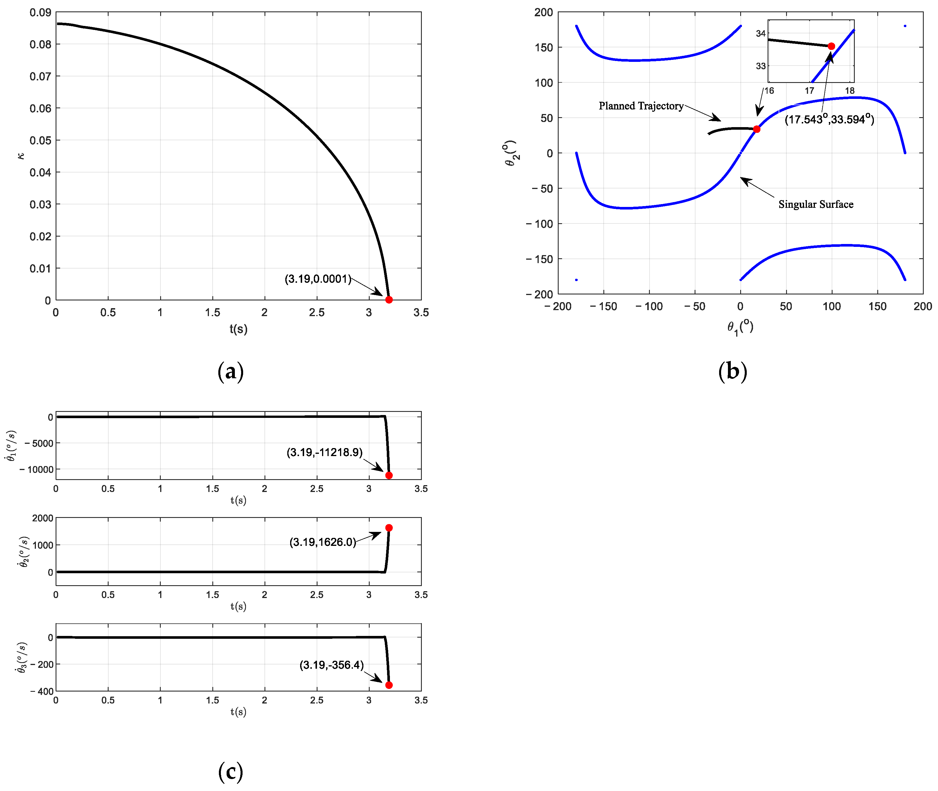
First, we present the simulation results without singularity avoidance, as shown in Figure 7. Figure 7a shows the variation in the singularity measure during path tracking. The singularity measure decreases rapidly and approaches zero at approximately 3.19 s, indicating that the system almost falls into a singular configuration. Figure 7b illustrates the relationship between the motion trajectory and the singular surface, revealing that joint angle state at this moment have nearly reached the singular surface, thereby confirming the system’s singular configuration. From the joint angular velocity command curve in Figure 7c, it can be seen that the commanded angular velocity at the singular moment exceeds 11000°/s, far beyond the practical engineering range, causing the actual joint motion to get “stuck” at this point, unable to complete the remaining motion process of the desired path.

Figure 7. Path planning results without singularity avoidance. (a) Singularity measure curve. (b) Trajectory in the joint space. (c) Joint angular velocity command.

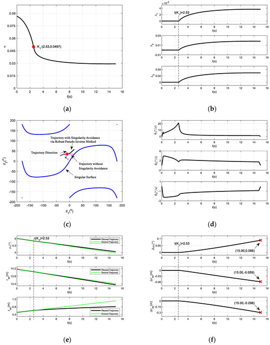
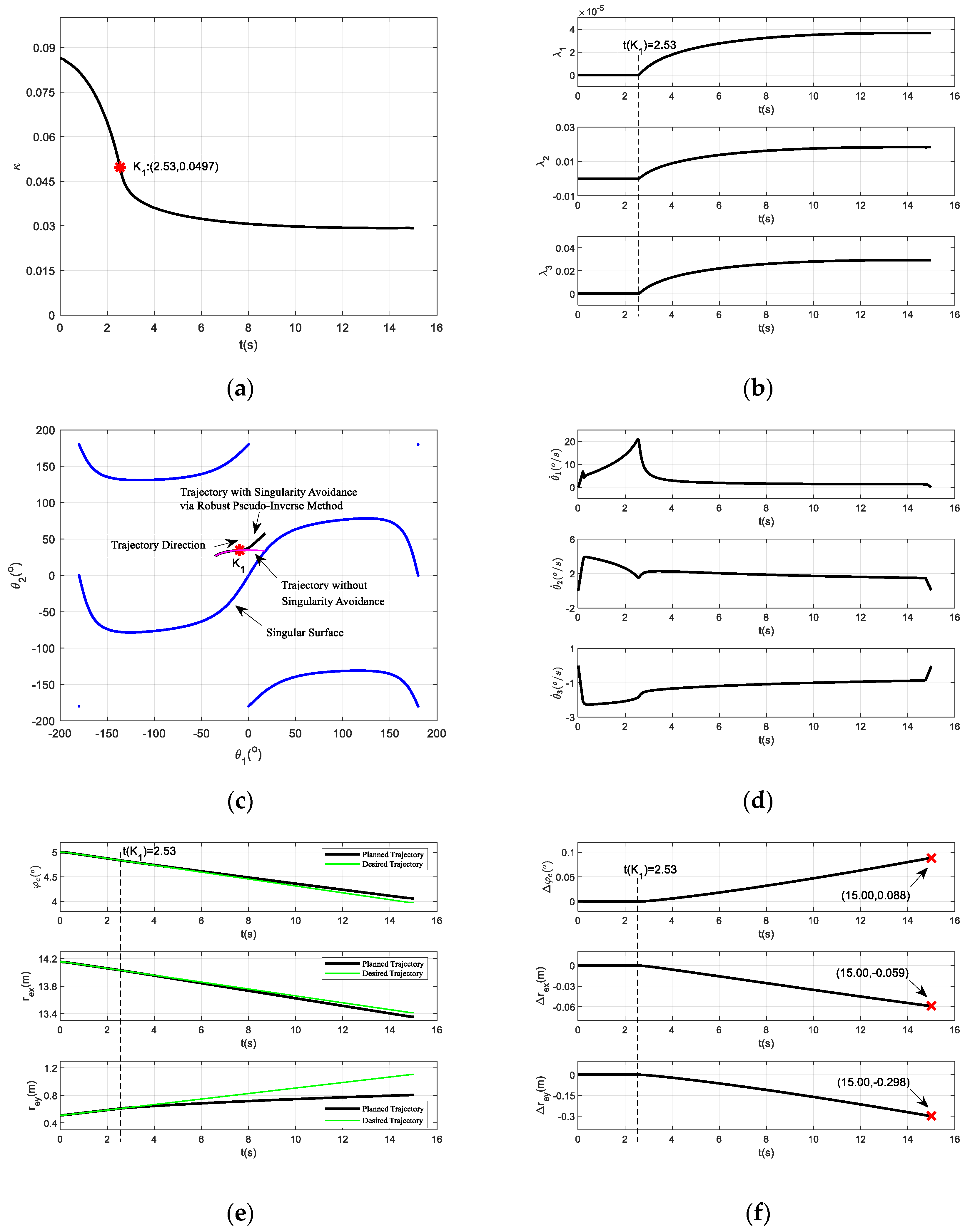
Figure 8 shows the planning results for singularity avoidance using the robust pseudo-inverse method. In the example, the singularity measure threshold is set to ${\kappa }_0$ = 0.05, and the maximum damping factors are taken as ${\lambda }_{m,1}^2$ = 0.0001, ${\lambda }_{m,2}^2$ = 0.05, and ${\lambda }_{m,3}^2$ = 0.08. It can be seen from Figure 8a that the singularity measure of the system remains above 0.025 throughout the whole process, staying at a certain distance from the singular configuration, but it cannot always remain above the threshold ${\kappa }_0$; from point $K_1$ at 2.53 s until the end of the motion, the singularity measure remains continuously below the threshold ${\kappa }_0$. At this point, damping factors ${\lambda }_i^2$ (i = 1, 2, 3) are introduced, with their values shown in Figure 8b. Point $K_1$ is denoted as the singularity-avoidance critical point. Figure 8c illustrates the relationship between the trajectory and the singular surface. It can be observed that, compared with the trajectory without singularity avoidance, the trajectory of the robust pseudo-inverse method, starting from the critical point $K_1$, slows down the approach toward the singular surface under the effect of the damping factors. It then continues to move closely along the singular surface, neither getting too close nor moving away. Figure 8d displays the joint angular velocity commands based on the robust pseudo-inverse method. The figure shows that the joint angular commands remain relatively smooth throughout, with magnitudes within a reasonable engineering range. Figure 8e,f show the actual end-effector pose throughout the process and the errors between the actual and desired values. As shown in the figure plots, starting from the critical point $K_1$, with the introduction of the damping factors, certain tracking errors are continuously introduced into the end-effector pose. The maximum errors throughout the process occur at the terminal moment, with values of 0.088°, −0.059 m, and −0.298 m, respectively. Such errors may be unacceptable for robotic tasks requiring high precision.

Figure 8. Path planning results with singularity avoidance via robust pseudo-inverse method. (a) Singularity measure curve. (b) Damping factors curve. (c) Trajectory in the joint space. (d) Joint angular velocity command. (e) End-effector pose. (f) Errors of the end-effector pose.

In summary, the robust pseudo-inverse method can achieve basic singularity avoidance, but it has two shortcomings: First, it can only ensure that the inverse kinematics of the system is solvable, but it lacks the ability to actively steer the system away from singularities; second, when approaching a singular region, obtaining feasible joint motion commands comes at the cost of introducing path tracking errors, thereby reducing planning accuracy. Since it lacks the ability to actively avoid singularities, the system may remain in a singular configuration continuously under the robust pseudo-inverse method, which in turn continuously introduces errors, and may eventually lead to excessive errors that are unacceptable.

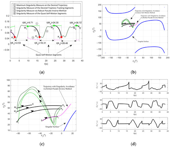
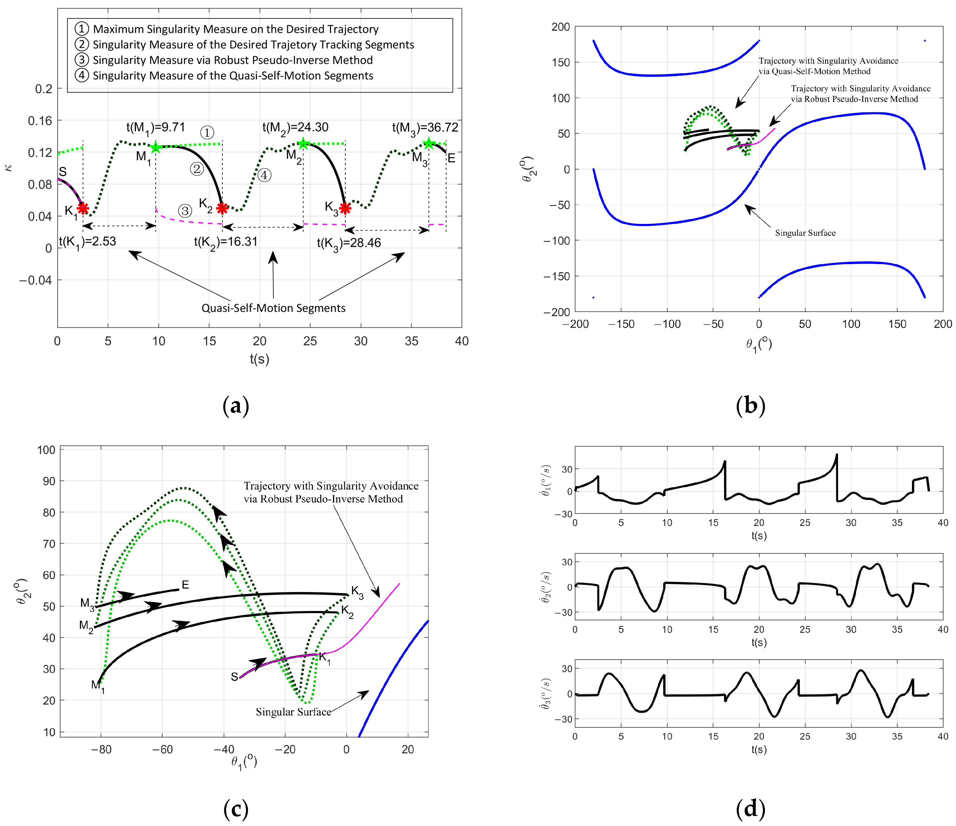
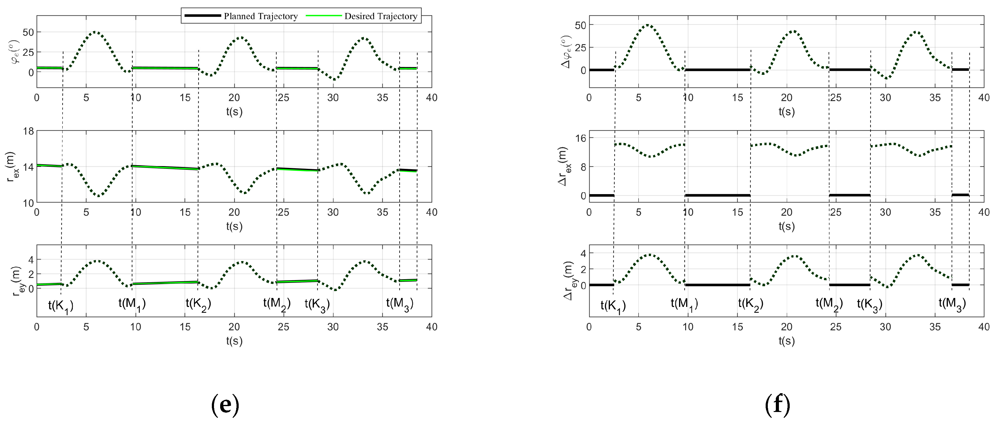
Finally, we examine the path planning effect for singularity avoidance using the quasi-self-motion method proposed in this paper. In the simulation, the singularity measure threshold is set equal to that of the robust pseudo-inverse method; i.e., ${\kappa }_0$ = 0.05. A quasi-self-motion adjustment is applied whenever the system’s singularity measure falls below the threshold ${\kappa }_0$. The simulation results are shown in Figure 9. Figure 9a shows that after the system starts moving from the starting point $S$, at $K_1$ at 2.53 s, the singularity measure is $\kappa$ = 0.0497, falling below the threshold ${\kappa }_0$ for the first time. At this point, a quasi-self-motion $\stackrel{⏜}{K_1{M}_1}$ is inserted to reconfigure the joint angle state. At the start of reconfiguration, the base attitude is ${\phi }_0=-10.1°$, with joint angles of $\mathit{\theta }={\left(\begin{array}{ccc}-9.6°& 34.6°& -10.2°\end{array}\right)}^T$, corresponding to an end-effector pose of ${\mathit{X}}_{\mathrm{e}}\left(t_0\right)={\left(\begin{array}{ccc}4.8°& 14.031 \mathrm{m}& 0.609 \mathrm{m}\end{array}\right)}^T$. The reconfiguration quasi-self-motion process takes 7.18 s and completes at $M_1$ at 9.71 s. At completion, the base attitude and joint angles are ${\phi }_0=64.2°$ and $\mathit{\theta }={\left(\begin{array}{ccc}-80.8°& 25.3°& -3.7°\end{array}\right)}^T$, respectively, while the end-effector pose remains the same as at the beginning of reconfiguration. After reconfiguration, the system singularity measure increases significantly to $\kappa$ = 0.1257. After reconfiguration, the singularity measure remains large for a long time until $K_2$ at 16.31 s, when it again falls below the threshold ${\kappa }_0$, triggering a second reconfiguration process. The entire motion process involved three reconfiguration phases. Taking the second segment $\stackrel{⏜}{M_1{K}_2}$ of the desired path of the end-effector pose as an example, in Figure 9a: Point ① represents the maximum singularity measure at each point on this desired path. The curve shows that the maximum singularity measure at each point is relatively large, indicating that whenever the system falls into singularity at any point on the desired path, it can be reconfigured to a state significantly far from singularity via quasi-self-motion. Point ② is the singularity measure of the actual motion. Point ③ is the corresponding singularity measure from the robust pseudo-inverse method shown in Figure 8a. A comparison of the two reveals that the singularity measure of the quasi-self-motion method is significantly greater than the latter and consistently remains above the threshold ${\kappa }_0$. Point ④ represents the quasi-self-motion process that adjusts the singularity measure to the maximum singularity measure state for the current end-effector pose after a singularity is encountered. This process is implemented using the Basis Algorithm based on forward kinematics, which has no singularity issue. Figure 9b illustrates the process in the joint space where the three quasi-self-motions move the system away from the singular surface, and Figure 9c provides a close-up view of this process. Both figures clearly show that after falling into a singular configuration, the planning result of the quasi-self-motion method is significantly farther away from the singular region than that of the robust pseudo-inverse method. Figure 9d shows the planned joint angular velocity commands. Throughout the process, the joint angular velocity does not exceed 50°/s, always staying within a reasonable engineering range. Figure 9e,f show the end-effector pose and its errors during the entire process. As can be seen from the figures, except for the quasi-self-motion segments for singularity reconfiguration, the end-effector tracking errors remain 0 throughout the other motion segments where the end-effector pose track the desired path, effectively ensuring tracking accuracy.

Figure 9. Path planning results with singularity avoidance via quasi-self-motion method. (a) Singularity measure curve. (b) Trajectory in the joint space. (c) Motion analysis of trajectory in the joint space. (d) Joint angular velocity command. (e) End-effector pose. (f) Errors of the end-effector pose.

The quasi-self-motion method achieves singular state regulation by introducing a joint reconfiguration process, which incurs an additional time cost; the increase in time is primarily related to the joint angular velocity and the adjustment amplitude. In this simulation, three reconfiguration segments—$\stackrel{⏜}{K_1{M}_1}$, $\stackrel{⏜}{K_2{M}_2}$, $\stackrel{⏜}{K_3{M}_3}$—were introduced, as shown in Table 2. The maximum joint angle amplitudes for the three reconfiguration adjustments were approximately 71.2°, 79.7°, and 82.5°, respectively. At joint angular velocities not exceeding 50°/s, as shown in Figure 9d, the additional times were 7.18 s, 7.99 s, and 8.26 s, respectively. Considering a maximum reconfiguration joint angle amplitude of 180°, the estimated maximum time increase due to reconfiguration is no more than 30 s. For engineering tasks such as on-orbit assembly and maintenance, as well as on-orbit refueling, this time cost is acceptable.

Table 2. Simulation results for reconfiguration segments.

No.	Pre-Reconfiguration State		Post-Reconfiguration State		Reconfiguration Duration(s)
	Base Attitude Angle (°)	Joint Angles (°)	Base Attitude Angle (°)	Joint Angles (°)
$\mathrm{Segment} 1 \stackrel{⏜}{K_1{M}_1}$	−10.0	(−9.6, 34.6, −10.2)	64.2	(−80.8, 25.3, −3.7)	7.18
$\mathrm{Segment} 2 \stackrel{⏜}{K_2{M}_2}$	−22.2	(−2.5, 48.0, −18.7)	57.5	(−82.2, 43.1, −13.7)	7.99
$\mathrm{Segment} 3 \stackrel{⏜}{K_3{M}_3}$	−27.1	(0.7, 53.7, −22.9)	54.7	(−81.8, 49.6, −18.1)	8.26

In summary, the quasi-self-motion method is effective in avoiding singularities. Compared with the robust pseudo-inverse method, its principal advantages are active singularity escape, maintenance of the singularity measure above the prescribed threshold, and zero path-tracking errors. However, a limitation of this method is that quasi-self-motion cannot be performed simultaneously with the motion of tracking the desired path, thus extending the total duration of the entire process. Whether quasi-self-motion can be performed simultaneously with desired path tracking, and how to achieve it, is a direction for future research.

7. Conclusions

This paper investigates the singularity problem in path planning for the end-effector pose of an FFSR. Based on the kinematic modeling of the system, the resolved motion rate control for the end-effector pose path planning is presented, and the singularity problem encountered therein is identified.

Subsequently, an analysis of singularity characteristics is conducted, identifying the factors influencing singularity and proving that singularity is independent of the base attitude. On this basis, a method for calculating singular surface is proposed, and the singular surface in the joint space is plotted to provide an intuitive visualization of the system’s singularities. Based on the plotted results, the symmetry of the singular surface is conjectured and proved.

Finally, a quasi-self-motion singularity-avoidance method based on joint configuration reconstruction is proposed, which is a novel approach for singularity avoidance in nonholonomic systems. The paper first defines and analyzes the general existence of quasi-self-motion, then presents the detailed design process for singularity avoidance using this method, and finally computes the end-effector pose space where quasi-self-motion does not exist.

Numerical simulations validate the effectiveness of the quasi-self-motion method for singularity avoidance. A comparison with the robust pseudo-inverse method demonstrates that the quasi-self-motion method offers significant advantages of actively escaping singularities, ensuring that the singularity measure always remains above a set threshold, and introducing no tracking errors. A limitation is that quasi-self-motion cannot be performed simultaneously with desired path tracking, thereby increasing the total duration of the entire process. For this reason, the proposed method is mainly applicable to path planning scenarios for cooperative targets with fixed target poses, and cannot be applied to that for non-cooperative targets whose target poses are unfixed or even unpredictable. Whether quasi-self-motion can be achieved simultaneously with desired trajectory tracking without incurring additional planning time, and how to realize it, constitute the direction of future research.

References

- Rybus, T. Robotic Manipulators for In-Orbit Servicing and Active Debris Removal: Review and Comparison. Prog. Aerosp. Sci. 2024, 151, 101055. [Google Scholar] [CrossRef] [Scilit]
- Zhang, W.; Li, F.; Li, J.; Cheng, Q. Review of On-Orbit Robotic Arm Active Debris Capture Removal Methods. Aerospace 2023, 10, 13. [Google Scholar] [CrossRef] [Scilit]
- Fallahiarezoodar, N.; Zhu, Z. Review of Autonomous Space Robotic Manipulators for On-Orbit Servicing and Active Debris Removal. Space Sci. Technol. 2025, 5, 0291. [Google Scholar] [CrossRef] [Scilit]
- Nair, M.H.; Rai, M.C.; Poozhiyil, M.; Eckersley, S.; Kay, S.; Estremera, J. Robotic Technologies for In-Orbit Assembly of a Large Aperture Space Telescope: A Review. Adv. Space Res. 2024, 74, 5118–5141. [Google Scholar] [CrossRef] [Scilit]
- Wang, Z.; Wang, P.; Duan, J.; Tian, W. Review of On-Orbit Assembly Technology with Space Robots. Aerospace 2025, 12, 375. [Google Scholar] [CrossRef] [Scilit]
- Carignan, C.R.; Detry, R.; Saaj, M.C.; Marani, G.; Vander Hook, J.D. Robotic In-Situ Servicing, Assembly and Manufacturing. Front. Robot. AI 2022, 9, 887506. [Google Scholar] [CrossRef] [Scilit] [PubMed]
- Papadopoulos, E.; Aghili, F.; Ma, O.; Lampariello, R. Robotic Manipulation and Capture in Space. Front. Robot. AI 2022, 9, 849288. [Google Scholar] [CrossRef] [Scilit] [PubMed]
- Ma, B.; Jiang, Z.; Liu, Y.; Xie, Z. Advances in Space Robots for On-Orbit Servicing: A Comprehensive Review. Adv. Intell. Syst. 2023, 5, 2200397. [Google Scholar] [CrossRef] [Scilit]
- Xu, W.; Liang, B.; Xu, Y. Survey of Modeling, Planning, and Ground Verification of Space Robotic Systems. Acta Astronaut. 2011, 68, 1629–1649. [Google Scholar] [CrossRef] [Scilit]
- Huang, X.; Xu, S. Free Floating Space Robot Kinematic Modeling and Analysis. Adv. Astronaut. Sci. 2014, 150, 2067–2077. [Google Scholar]
- Wang, M.; Luo, J.; Zheng, L.; Yuan, J.; Walter, U. Generate Optimal Grasping Trajectories to the End-Effector Using an Improved Genetic Algorithm. Adv. Space Res. 2020, 66, 1803–1817. [Google Scholar] [CrossRef] [Scilit]
- Dulęba, I.; Karcz-Dulęba, I. Many Faces of Singularities in Robotics. Pomiary Autom. Robot. 2023, 27, 19–26. [Google Scholar] [CrossRef] [Scilit]
- Ratajczak, J.; Tchoń, K. Normal Forms and Singularities of Non-Holonomic Robotic Systems: A study of Free-Floating Space Robots. Syst. Control Lett. 2020, 138, 104661. [Google Scholar] [CrossRef] [Scilit]
- Chen, G.; Zhang, L.; Jia, Q.; Sun, H. Singularity Analysis of Redundant Space Robot with the Structure of Canadarm2. Math. Probl. Eng. 2014, 2014, 735030. [Google Scholar] [CrossRef] [Scilit]
- Papadopoulos, E.; Dubowsky, S. Dynamic Singularities in Free-Floating Space Manipulators. J. Dyn. Sys. Meas. Control 1993, 115, 44–52. [Google Scholar] [CrossRef] [Scilit]
- Wang, M.; Luo, J.; Fang, J.; Yuan, J. Optimal Trajectory Planning of Free-Floating Space Manipulator Using Differential Evolution Algorithm. Adv. Space Res. 2018, 61, 1525–1536. [Google Scholar] [CrossRef] [Scilit]
- Huang, X.; Zhao, Q.; Bai, W. Trajectory Planning of a Free-Floating Manipulator with Singularity Analysis and Avoidance. Aerosp. Control 2024, 42, 15–22. (In Chinese) [Google Scholar]
- Tchoń, K.; Ratajczak, J. Singularities of Holonomic and Non-Holonomic Robotic Systems: A Normal Form Approach. J. Frankl. Inst. 2021, 358, 7698–7713. [Google Scholar] [CrossRef] [Scilit]
- Gasparetto, A.; Boscariol, P.; Lanzutti, A.; Vidoni, R. Trajectory Planning in Robotics. Math. Comput. Sci. 2012, 6, 269–279. [Google Scholar] [CrossRef] [Scilit]
- Ni, S.; Chen, W.; Ju, H.; Chen, T. Coordinated Trajectory Planning of a Dual-Arm Space Robot with Multiple Avoidance Constraints. Acta Astronaut. 2022, 195, 379–391. [Google Scholar] [CrossRef] [Scilit]
- Zhang, H.; Zhu, Z. Sampling-Based Motion Planning for Free-Floating Space Robot without Inverse Kinematics. Appl. Sci. 2020, 10, 9137. [Google Scholar] [CrossRef] [Scilit]
- Calzolari, D.; Lampariello, R.; Giordano, A.M. Singularity maps of space robots and their application to gradient-based trajectory planning. In Proceedings of the 16th Robotics: Science and Systems Conference (RSS 2020), Online, 12–16 July 2020. [Google Scholar]
- Jin, R.; Geng, Y.; Xie, X.; Zhong, C.; Huang, Y.; Geng, Y. Deep Reinforcement Learning-Based Trajectory Planning for Space Robots Avoiding Dynamic Singularities. IFAC-PapersOnLine 2025, 59, 327–332. [Google Scholar] [CrossRef] [Scilit]
- Xi, F.; Fenton, R.G. On the Inverse Kinematics of Space Manipulators for Avoiding Dynamic Singularities. J. Dyn. Sys. Meas. Control 1997, 119, 340–346. [Google Scholar] [CrossRef] [Scilit]
- Wu, J.; Bin, D.; Feng, X.; Wen, Z.; Zhang, Y. GA Based Adaptive Singularity-Robust Path Planning of Space Robot for On-Orbit Detection. Complexity 2018, 2018, 3702916. [Google Scholar] [CrossRef] [Scilit]
- Rousso, P.; Chhabra, R. Singularity-Robust Full-Pose Workspace Control of Space Manipulators with Non-Zero Momentum. Acta Astronaut. 2023, 208, 322–342. [Google Scholar] [CrossRef] [Scilit]
- Cocuzza, S.; Rossi, S.; Debei, S. Novel Reaction Control of Space Manipulators with Increased Robustness against Singularities and Physical Joint Limits. In Proceedings of the 63th International Astronautical Congress (IAC), Naples, Italy, 1–5 October 2012. [Google Scholar]
- Mansfeld, N.; Michel, Y.; Bruckmann, T.; Haddadin, S. Improving the Performance of Auxiliary Null Space Tasks via Time Scaling-Based Relaxation of the Primary Task. In Proceedings of the 2019 IEEE International Conference on Robotics and Automation (ICRA), Montreal, QC, Canada, 20–24 May 2019; pp. 9342–9348. [Google Scholar]
- Zhou, C.; Jin, M.; Liu, Y.; Zhang, Z.; Liu, Y.; Liu, H. Singularity Robust Path Planning for Real Time Base Attitude Adjustment of Free-Floating Space Robot. Int. J. Autom. Comput. 2017, 14, 169–178. [Google Scholar] [CrossRef] [Scilit]
- Li, Y.; Wang, L. Comprehensive Research and Analysis on Obstacle-Singularity-Joint Limit Avoidance of Redundant Robot. Int. J. Adv. Robot. Syst. 2024, 21, 17298806241233910. [Google Scholar] [CrossRef] [Scilit]
- Murray, R.M.; Li, Z.; Sastry, S.S. A Mathematical Introduction to Robotic Manipulation; CRC Press: Boca Raton, FL, USA, 2017; pp. 321–331. [Google Scholar]
- Vafa, Z.; Dubowsky, S. On the Dynamics of Space Manipulators Using the Virtual Manipulator, with Applications to Path Planning. J. Astronaut. Sci. 1990, 38, 441–472. [Google Scholar]
- Fernandes, C.; Gurvits, L.; Li, Z. Near-Optimal Nonholonomic Motion Planning for a System of Coupled Rigid Bodies. IEEE Trans. Autom. Control 1994, 39, 450–463. [Google Scholar] [CrossRef] [Scilit]
- Blaise, J.; Bazzocchi, M.C.F. Space Manipulator Collision Avoidance Using a Deep Reinforcement Learning Control. Aerospace 2023, 10, 778. [Google Scholar] [CrossRef] [Scilit]
- Li, Y.; Li, D.; Zhu, W.; Sun, J.; Zhang, X.; Li, S. Constrained Motion Planning of 7-DOF Space Manipulator via Deep Reinforcement Learning Combined with Artificial Potential Field. Aerospace 2022, 9, 163. [Google Scholar] [CrossRef] [Scilit]
Disclaimer/Publisher’s Note: The statements, opinions and data contained in all publications are solely those of the individual author(s) and contributor(s) and not of MDPI and/or the editor(s). MDPI and/or the editor(s) disclaim responsibility for any injury to people or property resulting from any ideas, methods, instructions or products referred to in the content. |
© 2026 by the authors. Licensee MDPI, Basel, Switzerland. This article is an open access article distributed under the terms and conditions of the Creative Commons Attribution (CC BY) license.