


Abstract
Automatic Dependent Surveillance–Broadcast (ADS-B) is a key source of air traffic surveillance data, but its open broadcast mechanism and possible trajectory-data inconsistencies may reduce surveillance reliability. This study proposes a Short-window Temporal Latent-Consistency Network (STLC-Net) for window-level anomaly detection in real-world ADS-B surveillance data. Raw ADS-B messages are transformed into physically interpretable kinematic features and segmented into short sliding windows to capture local motion inconsistencies. STLC-Net combines LSTM-based temporal encoding with an encoder–decoder–encoder latent-consistency mechanism, and fuses reconstruction and latent-consistency discrepancies to produce anomaly scores. Experimental results show that STLC-Net achieves a PR-AUC of 0.952540, precision of 1.0, recall of 0.882682, and F1-score of 0.937685 under highly imbalanced conditions. Ablation studies further confirm the effectiveness of short-window representation, temporal modeling, and latent-consistency learning. These results indicate that STLC-Net provides an effective and physically interpretable framework for detecting rare kinematic anomalies in ADS-B trajectory surveillance data.
1. Introduction
Automatic Dependent Surveillance–Broadcast (ADS-B) has become an important data source for modern air traffic surveillance. By periodically broadcasting aircraft identity, position, altitude, speed, heading, and other flight-state information, ADS-B supports traffic monitoring, trajectory analysis, and situational awareness. Nevertheless, abnormal trajectory observations may arise from receiver faults, navigation errors, message corruption, unusual flight maneuvers, environmental disturbances, or deliberate data manipulation. Because basic ADS-B messages generally lack built-in encryption and authentication mechanisms, the reliability of a received trajectory cannot be determined from message reception alone. Detecting kinematic inconsistencies in continuous ADS-B trajectories is therefore important for maintaining reliable surveillance and supporting subsequent operational assessment.
Existing studies have investigated ADS-B reliability from both security and data-driven anomaly-detection perspectives. Prior work has analyzed vulnerabilities to message injection, modification, spoofing, and replay attacks [1,2]. LSTM encoder–decoder models have been used to learn legitimate route patterns and identify anomalous ADS-B messages through reconstruction errors [3], while autoencoder-based methods have been applied to airborne attack detection [4]. Other studies have addressed specific scenarios through physical-layer spoofing detection [5], supervised false-data-injection detection [6], GAN-LSTM-based attack detection [7], and dual-domain trajectory modeling with reversible normalization and spectral patch attention [8]. These studies demonstrate the potential of learning-based ADS-B monitoring. However, many existing methods focus on predefined attacks, individual messages, route-specific patterns, or relatively long sequence representations. Rare and short-term kinematic inconsistencies in real surveillance trajectories therefore require further investigation.
Anomaly detection has been extensively studied across different application domains [9], and recent surveys have summarized the development of machine learning and deep learning methods for time-series anomaly detection [10,11]. Recurrent reconstruction models can capture temporal dependencies [12,13], while multivariate and adversarial approaches can model complex temporal and inter-variable relationships [14,15,16]. However, ADS-B trajectory variables have explicit physical meanings, and an anomaly may appear only as a brief inconsistency in speed, heading, altitude, or displacement. A long input sequence may dilute such a local deviation, whereas reconstruction error alone may not fully characterize abnormal changes in the learned representation. An effective ADS-B trajectory detector should therefore combine motion-aware features, short-window temporal modeling, and a representation-level anomaly criterion, while being evaluated carefully under severe class imbalance.
To address these issues, this paper proposes a Short-window Temporal Latent-Consistency Network (STLC-Net) for window-level anomaly detection in real ADS-B surveillance data. Raw ADS-B messages are transformed into 24 physically interpretable kinematic features and segmented into short sliding windows to preserve local motion evolution. STLC-Net adopts an LSTM-based encoder–decoder–encoder structure inspired by GANomaly [17]. Unlike a conventional LSTM autoencoder that relies only on reconstruction discrepancy, STLC-Net evaluates each trajectory window using both reconstruction discrepancy and latent-space consistency. Unlike non-recurrent GANomaly implementations, its recurrent modules preserve the temporal order within each trajectory window. Based on the corresponding ablation results, the final model is trained using reconstruction and latent-consistency losses without adversarial regularization.
The main contributions of this study are summarized as follows:
- A window-level ADS-B trajectory anomaly-detection framework is developed by integrating physically interpretable kinematic feature construction, short-window trajectory representation, and a model-independent rule-based procedure for generating reference anomaly labels.
- STLC-Net combines LSTM-based temporal modeling with an encoder–decoder–encoder latent-consistency mechanism, allowing abnormal trajectory windows to be assessed from both reconstruction and representation-consistency perspectives.
- Comprehensive comparative and supplementary experiments are conducted under a validation-based threshold-selection protocol. The results validate the effectiveness and stability of STLC-Net for short-window ADS-B trajectory anomaly detection.
2. Related Work
2.1. ADS-B Anomaly Detection
Due to the open and unauthenticated broadcast mechanism of ADS-B, previous studies have examined its vulnerability to message injection, modification, spoofing, replay attacks, and other security threats [1,2]. Existing data-driven detection methods can generally be divided into trajectory reconstruction and sequence modeling, attack-specific detection, and operational-event identification.
Reconstruction- and sequence-based methods learn normal flight behavior and identify deviations from the learned patterns. Habler and Shabtai employed an LSTM encoder–decoder to model legitimate flight routes and detect anomalous ADS-B messages using reconstruction errors [3]. Wang et al. applied sliding-window LSTM modeling to ADS-B spoofing detection [18]. Fried and Last evaluated autoencoder-based models against different airborne attacks, demonstrating the applicability of reconstruction learning to ADS-B security monitoring [4]. These methods exploit temporal dependencies in consecutive ADS-B observations, but their detection decisions are mainly based on reconstruction or prediction discrepancies.
Other studies have developed detectors for particular attack types or data representations. Ying et al. proposed a deep neural network-based framework that uses physical-layer information to detect ADS-B spoofing [5]. Karam et al. constructed false-data samples and trained a supervised model to detect manipulated ADS-B fields [6]. Yue et al. combined generative adversarial learning with LSTM-based temporal modeling for ADS-B attack detection [7], while Kacem and Tossou introduced a Transformer-based method for replay-attack detection [19]. More recently, RDPA incorporated reversible normalization and spectral patch attention to model ADS-B trajectories in temporal and frequency-related representations [8]. These approaches improve detection for their respective settings, although many rely on predefined attack patterns, supervised labels, or task-specific input representations.
ADS-B trajectories have also been used to identify safety-related operational events. Proud detected go-around events using crowd-sourced ADS-B position data [20], and Kumar et al. further classified and analyzed commercial-aviation go-arounds from ADS-B trajectories [21]. Such studies demonstrate that trajectory evolution contains useful information for recognizing unusual flight behavior, but their objectives are generally limited to specific operational events rather than general anomaly detection.
Overall, existing studies support the feasibility of learning-based ADS-B monitoring, but several limitations remain. Many methods focus on isolated messages, predefined attacks, specific flight routes, or known operational events, whereas anomalies in real surveillance data may appear as rare and short-term kinematic inconsistencies within continuous trajectories. In addition, a detected trajectory deviation should be interpreted as an observable kinematic anomaly rather than direct evidence of a particular cause, because similar patterns may arise from equipment faults, navigation errors, unusual maneuvers, data corruption, or deliberate manipulation. The present study therefore focuses on short-window trajectory anomaly screening rather than attack attribution or source authentication.
2.2. Trajectory Anomaly Detection Using Other Flight Data Sources
In addition to ADS-B, trajectory anomaly detection has been investigated using surveillance radar tracks, Global Positioning System (GPS) measurements, and onboard flight-recording data. These data sources differ in their observation mechanisms, sampling characteristics, and available flight variables, but they share the objective of identifying deviations from expected aircraft motion or operational patterns.
For ground-based surveillance data, Matthews et al. developed an automated process for discovering unusual flight-track profiles in complex terminal airspace using radar-track and related operational data, with domain-expert assessment used to examine the operational significance of the detected events [22]. Cao et al. combined a multi-dimensional outlier descriptor with a bidirectional LSTM network to detect track deviations and track outliers from real aircraft track data [23]. These studies indicate that multi-dimensional spatial and temporal information from aircraft tracks can support the identification of unusual flight profiles. Nevertheless, a detected track deviation does not necessarily reveal whether it originates from an operational maneuver, a measurement error, or another underlying cause.
GPS-based studies frequently focus on navigation integrity and spoofing-induced trajectory deviations. Huang et al. proposed a stacked-LSTM trajectory prediction model and an ensemble-voting detector for UAV GPS spoofing. Position anomalies were identified by comparing predicted motion states with observed trajectory information, enabling the online detection of spoofing-induced deviations [24]. Compared with external surveillance sources, onboard Flight Data Recorder (FDR) data provide additional variables related to aircraft states, system operation, and pilot control. Li and Hansman applied clustering analysis to routine FDR data to identify abnormal flights and operational patterns that were not covered by predefined exceedance rules [25].
Overall, radar tracks, GPS measurements, and onboard flight data provide complementary perspectives on flight anomaly detection. Radar and GPS data mainly characterize aircraft motion and navigation behavior, whereas onboard data contain more detailed information about aircraft systems and control states. However, differences in data accessibility, sampling frequency, feature definitions, and anomaly labels make direct comparison and model transfer across these data sources difficult. The present study therefore focuses on short-term kinematic anomaly screening from ADS-B trajectory windows, while the integration of radar, navigation, and onboard data remains a valuable direction for improving anomaly interpretation and cause attribution.
2.3. Deep Learning for Time-Series Anomaly Detection
Time-series anomaly detection aims to identify observations or subsequences that deviate from normal temporal patterns. Classical surveys have summarized general anomaly detection settings and evaluation issues [9], while recent reviews have focused on outlier detection and deep learning-based methods for time-series data [10,11]. Reconstruction-based models are widely used because they learn normal representations and measure abnormality through reconstruction discrepancies.
Recurrent models have been widely adopted for sequential monitoring. Malhotra et al. proposed an LSTM encoder–decoder framework for multi-sensor anomaly detection [12], and Hundman et al. combined LSTM models with dynamic thresholding for spacecraft telemetry anomaly detection [13]. For multivariate time series, OmniAnomaly models temporal dynamics with a stochastic recurrent neural network [14], MSCRED captures multi-scale temporal patterns and sensor correlations through convolutional and recurrent structures [15], and USAD employs adversarially trained autoencoders for unsupervised anomaly detection [16]. These methods show that temporal dependence and inter-variable relationships are important for detecting abnormal patterns in sequential data.
Attention-based and Transformer-based models have also been introduced into time-series anomaly detection following the success of the Transformer architecture in sequence modeling [26]. For example, Anomaly Transformer uses association discrepancy to identify anomalous time points [27], while TranAD adopts Transformer-based sequence encoders for multivariate anomaly detection and diagnosis [28]. In the aviation domain, Ayhan et al. explored the Temporal Fusion Transformer for anomaly detection in multivariate flight time-series data by learning nominal flight behavior and identifying deviations between forecasted and observed flight parameters [29]. These models provide useful ideas for capturing long-range dependencies and complex variable interactions.
Class imbalance is another important issue in aviation-safety learning because safety-related events generally account for only a small proportion of available observations. Zhou et al. combined data augmentation with an imbalance-aware hybrid loss function for helicopter-accident fatality prediction [30]. Hou et al. proposed a text-mining and selective-ensemble framework for the highly imbalanced identification of civil-aviation maintenance hazards [31]. These studies indicate that data-level augmentation and algorithm-level imbalance treatments can improve the learning of rare aviation-safety events. However, they mainly address supervised tasks with labeled minority-class samples, whereas the present study adopts a one-class setting in which the model representation is learned from normal trajectory windows.
Although these studies provide important methodological foundations, ADS-B anomaly detection has distinct domain characteristics. ADS-B trajectories contain physically meaningful flight states, and anomalies are often reflected by abrupt changes in altitude, speed, heading, or horizontal displacement. Therefore, ADS-B anomaly detection requires both temporal dependency modeling and motion-aware feature representation, especially under highly imbalanced conditions.
2.4. Generative and Latent-Consistency-Based Anomaly Detection
Generative and representation learning models provide another important direction for anomaly detection. Deep generative anomaly detection methods, such as DAGMM and Donut, learn compact latent representations or probabilistic reconstruction patterns to identify samples that deviate from the normal data distribution [32,33]. In the time-series domain, LSTM-GAN combines LSTM networks with generative adversarial learning to model temporal dynamics [34]. MAD-GAN uses a GAN-based framework for multivariate time-series anomaly detection [35], while TadGAN incorporates LSTM-based generators, critics, and cycle-consistency learning for unsupervised time-series anomaly detection [36]. ALGAN further introduces an adjusted-LSTM GAN structure for time-series anomaly detection [37]. These studies indicate that combining temporal modeling with generative or representation learning structures can help capture complex data distributions.
GANomaly introduced an encoder–decoder–encoder architecture that combines reconstruction discrepancy with latent-space consistency for anomaly detection [17]. Compared with methods relying only on reconstruction errors, latent-consistency learning provides an additional representation-level criterion for measuring whether an input sample conforms to the learned normal distribution. This idea is useful for ADS-B trajectory anomaly detection because abnormal windows may lead to both reconstruction errors and inconsistencies between original and reconstructed latent representations.
Building on these studies, STLC-Net introduces the latent-consistency concept into short-window ADS-B trajectory modeling through recurrent temporal modules. In contrast to reconstruction-only sequence models and the original non-recurrent GANomaly architecture, the proposed method considers both temporal dependencies and representation consistency.
3. Method
3.1. Problem-Driven Framework for Short-Window ADS-B Anomaly Detection
This study formulates ADS-B trajectory monitoring as a one-class, window-level time-series anomaly detection problem rather than a point-wise classification task over isolated messages. A trajectory window is considered anomalous when its multivariate kinematic evolution deviates from the normal patterns learned by the model. Such observable deviations may arise from equipment faults, navigation errors, unusual flight maneuvers, data corruption, environmental disturbances, or deliberate manipulation. Therefore, STLC-Net is designed to screen for short-term kinematic anomalies rather than to determine their underlying causes or authenticate the source of ADS-B messages. Because a short-lived inconsistency may not be sufficiently characterized by an individual message, this study proposes a Short-window Temporal Latent-Consistency Network (STLC-Net) for ADS-B trajectory anomaly detection.
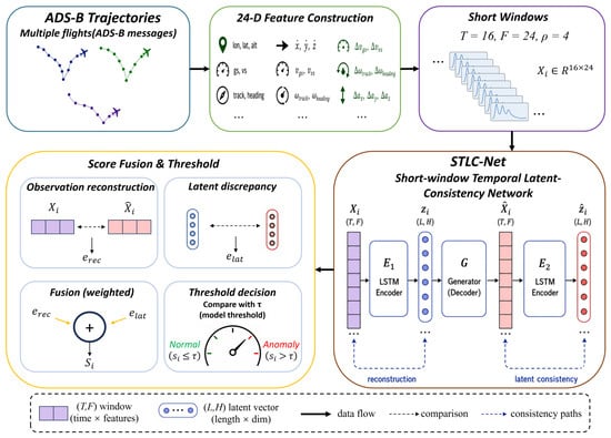
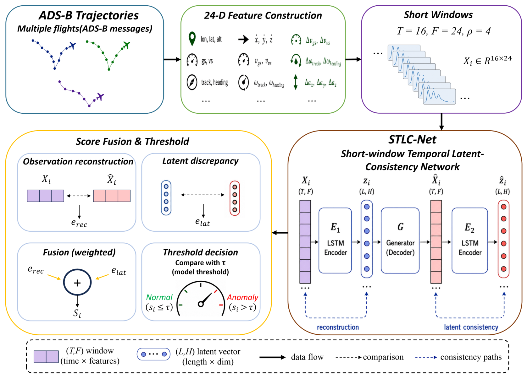
The overall framework is shown in Figure 1. Raw ADS-B messages are first transformed into physically interpretable kinematic feature vectors that describe flight states, local motion variations, and difference-enhanced motion information. The continuous trajectories are then segmented into fixed-length short windows using a sliding-window strategy, preserving local trajectory-evolution patterns. Each window is fed into STLC-Net, where an LSTM encoder captures short-term temporal dependencies, a decoder reconstructs the input window, and a secondary encoder constrains the reconstructed window in the latent space. Finally, reconstruction discrepancy and latent-consistency discrepancy are fused to obtain a window-level anomaly score.
Figure 1.
Overall framework of the proposed STLC-Net for short-window ADS-B trajectory anomaly detection. Raw ADS-B messages are transformed into kinematic features and segmented into short trajectory windows. STLC-Net combines LSTM-based temporal encoding with an encoder–decoder–encoder latent-consistency mechanism to compute reconstruction and latent-consistency discrepancies, which are fused into a window-level anomaly score.
The framework integrates short-window representation, recurrent temporal modeling, and latent-consistency learning. Short windows retain local kinematic variations while reducing the dilution of brief anomalies by longer normal trajectory segments. Compared with a conventional LSTM autoencoder that mainly evaluates reconstruction discrepancy, STLC-Net introduces a secondary encoder to provide an additional representation-consistency criterion. Compared with the original non-recurrent GANomaly architecture, the LSTM-based modules preserve the temporal order and local evolution of consecutive ADS-B observations. The respective contributions of these components are further examined through the ablation experiments.
For the i-th ADS-B trajectory window, the input is denoted as
where T is the window length and F is the feature dimension. In the main experimental setting, and . STLC-Net outputs a continuous anomaly score for each window. The final binary decision is obtained using a threshold selected exclusively from the validation set and subsequently fixed for test-set evaluation, as described in Section 3.5.
3.2. ADS-B Kinematic Feature Construction
Raw ADS-B messages provide basic flight-state information, including altitude, speed, heading, longitude, latitude, and timestamp. These variables were selected because they describe the principal vertical and horizontal motion states of an aircraft. Altitude characterizes vertical movement, while speed, heading, and position describe horizontal motion and trajectory direction. However, short-term anomalies are often reflected not only in the absolute values of these variables but also in inconsistent changes across consecutive messages. Therefore, first-order motion variations and difference-enhanced features are further constructed to characterize local trajectory continuity, abrupt kinematic changes, and variations in the rate of motion. The resulting feature set describes the trajectory from instantaneous flight states, local motion variations, and difference-enhanced motion information.
The heading angle is encoded using sine and cosine functions to avoid angular discontinuity around and :
where denotes the heading angle in degrees at time step t. During resampling, the sine and cosine components are interpolated, and the heading angle is recovered as
Longitude and latitude are transformed into local planar coordinates using a local tangent-plane approximation. For each trajectory segment, the first point is used as the reference position:
where and denote longitude and latitude in degrees, respectively. The horizontal displacement between consecutive messages is defined as
First-order motion variations are calculated as
where can represent altitude, speed, or spatial coordinates. For heading, the angular difference is wrapped into :
Difference-enhanced features are further constructed as
where denotes a component of the 12-dimensional basic kinematic feature vector .
For each ADS-B message at time step t, the final 24-dimensional feature vector is defined as
where
and
Here, and denote altitude and speed, respectively; and denote projected planar coordinates; denotes horizontal displacement; denotes first-order motion variation; and denotes the difference-enhanced variation of the corresponding feature.
Overall, the 24-dimensional feature vector describes ADS-B trajectory dynamics from instantaneous flight states, first-order motion variations, and difference-enhanced motion changes. This representation provides physically interpretable input for STLC-Net and supports the detection of local kinematic inconsistencies across consecutive ADS-B messages.
3.3. Short-Window Trajectory Representation and Normalization
After kinematic feature construction, consecutive ADS-B messages are organized into trajectory windows for time-series anomaly detection. For the m-th flight trajectory, the ordered feature sequence is denoted as
where is the number of ADS-B messages in the m-th trajectory and denotes the feature vector at time step t. To avoid artificial discontinuities between different flights, sliding windows are generated only within the same trajectory and are not allowed to cross flight boundaries.
Each trajectory is segmented into fixed-length short windows using a sliding-window strategy. The j-th window generated from the m-th trajectory is represented as
where T is the window length, F is the feature dimension, and is the standardized feature vector. The starting index of the j-th window is given by
where is the sliding stride. In the main experimental setting, , , and . After window generation, all trajectory windows are re-indexed as for model training and evaluation.
Short-window representation is adopted because the target anomalies in this study are defined as brief kinematic inconsistencies within continuous trajectories. Compared with a longer window, a short window contains less unrelated normal context and therefore reduces the possibility that local abnormal patterns are diluted. At the same time, it preserves the temporal relationships among consecutive ADS-B messages, allowing the recurrent model to characterize local changes in altitude, speed, heading, and spatial displacement. The influence of window length is further examined through the window-size ablation experiment.
To ensure comparable numerical scales across feature dimensions, all features are standardized before being fed into the model. The standardization statistics are computed only from the training set:
where is the k-th feature at time step t, and are the mean and standard deviation of the k-th feature calculated from the training set, and is a small constant used to avoid division by zero. The same statistics are applied to the validation and test sets to prevent information leakage.
After segmentation and standardization, each window retains the local temporal evolution of flight states and motion variations. The original ADS-B message-level monitoring problem is therefore transformed into a short-window trajectory anomaly detection problem, where each window serves as the input of STLC-Net and is assigned a continuous anomaly score.
3.4. STLC-Net Architecture
STLC-Net is a one-class recurrent latent-consistency model designed to learn normal patterns from short ADS-B trajectory windows. Its architecture is developed by combining the temporal modeling capability of an LSTM autoencoder with the encoder–decoder–encoder latent-consistency mechanism introduced in GANomaly. However, the final STLC-Net does not retain the complete adversarial structure of GANomaly: no discriminator is included, and the decoder is used only for trajectory reconstruction. The model consists of a primary LSTM encoder, a reconstruction decoder, and a secondary LSTM encoder, as described below.
Given an input window , the first encoder maps it into a latent temporal representation:
where . Here, L denotes the latent sequence length and H denotes the hidden dimension of the LSTM encoder, corresponding to the notation in Figure 1. Unlike a fully connected encoder that flattens the input window, preserves the temporal order of consecutive ADS-B messages and captures local flight-state evolution.
The decoder G reconstructs the input window from :
where is the reconstructed trajectory window. In Figure 1, G is denoted as generator (decoder) following the GANomaly notation, but in STLC-Net it serves as a reconstruction decoder. The reconstructed window is then mapped back into the latent space by the secondary encoder :
where .
The architectural differences among a conventional LSTM autoencoder, the original GANomaly, and STLC-Net can be summarized as follows. A conventional LSTM autoencoder generally contains a recurrent encoder and decoder and identifies anomalies mainly according to the reconstruction discrepancy between the input and reconstructed sequences. It preserves temporal dependencies but does not explicitly evaluate whether the reconstructed sequence remains consistent with the input in the latent space. GANomaly introduces a secondary encoder and an adversarial discriminator, allowing reconstruction, latent consistency, and adversarial learning to be jointly considered; however, its original convolutional architecture was developed primarily for image anomaly detection and does not explicitly model sequential order. STLC-Net retains the encoder–decoder–encoder latent-consistency structure but replaces the original non-recurrent encoding modules with LSTM-based temporal modules. It therefore evaluates ADS-B trajectory windows using both reconstruction discrepancy and latent-space discrepancy while preserving the temporal order of consecutive observations. Based on the ablation results, the final implementation excludes the discriminator and adversarial regularization, and uses reconstruction and latent-consistency objectives for model training.
3.5. Training Objective and Anomaly Scoring
STLC-Net is trained to reconstruct normal ADS-B trajectory windows while preserving latent-space consistency. Given an input window and its reconstruction , the reconstruction loss is defined as
where T is the window length and F is the feature dimension.
The latent-consistency loss measures the discrepancy between the original and reconstructed latent representations:
where , L is the latent sequence length, and H is the hidden dimension of the LSTM encoder. The total latent dimension can also be denoted as .
The overall training objective is
where controls the weight of latent-consistency learning. Although STLC-Net is inspired by GANomaly, adversarial loss is not included in the final training objective and is only evaluated in the ablation study.
During inference, the reconstruction discrepancy and latent-space discrepancy of the i-th trajectory window are calculated as
Because the two discrepancy components may have different numerical scales, they are normalized separately before score fusion. To avoid information leakage, the normalization parameters are estimated exclusively from the training-window scores:
where denotes the training-window set. For any training, validation, or test window, the normalized discrepancy scores are calculated using the same training-derived statistics:
The normalization statistics are not re-estimated using the validation or test data.
The final anomaly score is obtained by combining the two normalized discrepancy components:
where controls the relative contributions of reconstruction discrepancy and latent-space discrepancy. In the main experiments, is fixed at 0.8, and its influence is examined separately through the anomaly-score fusion analysis.
The decision threshold is determined exclusively from the validation set. Let
where denotes the q-quantile and denotes the validation-window set. The threshold that maximizes the validation-set F1-score is selected:
After selection, is fixed and applied directly to the independent test set without further adjustment. The final window-level prediction is
where denotes an anomalous window and denotes a normal window. Test labels are not used for score normalization, threshold selection, model selection, or calibration. ROC-AUC and PR-AUC are calculated directly from the continuous anomaly scores and are independent of the selected decision threshold.
3.6. Model-Independent Data-Rule Labeling Strategy
Because manually verified anomaly annotations are unavailable for the collected ADS-B trajectories, this study adopts a model-independent data-rule labeling strategy to provide a consistent reference for window-level evaluation. The labels are generated from physically interpretable kinematic variations and are independent of STLC-Net and all compared models, thereby avoiding model-dependent pseudo-label bias. The resulting labels indicate statistically unusual short-term motion patterns rather than confirmed causes or predefined attack categories.
For each standardized window, inverse standardization is first applied to recover the original physical scale. A rule-related feature vector is then constructed from motion-variation features that describe vertical motion, speed continuity, directional variation, and horizontal displacement. Specifically, the selected features include , , , horizontal displacement, , , , , , , , and . Altitude variation characterizes vertical-motion consistency, speed and heading variations reflect changes in motion magnitude and direction, and planar displacement variables describe horizontal trajectory continuity. Their difference-enhanced forms are included to emphasize abrupt changes in the evolution of these quantities.
For each selected feature within a window, the maximum absolute value, mean absolute value, and 95th percentile of the absolute values are calculated. The maximum captures the strongest local deviation, the mean describes the overall variation within the window, and the 95th percentile provides an upper-tail statistic that is less dependent on a single extreme point. These statistics form the window-level rule feature vector .
Robust statistics are estimated only from the training windows. Let and denote the median and median absolute deviation (MAD) of the aggregated rule features in the training set. The positive robust deviation of the i-th window is calculated as
where is a small constant used for numerical stability. The window-level rule score is defined as
To avoid information leakage, the rule threshold is determined using only the training-window rule scores:
where denotes the set of training rule scores and denotes the p-th quantile. In this study, is adopted as a conservative, training-data-driven cutoff for identifying windows located in the extreme upper tail of the kinematic rule-score distribution. This percentile is a dataset-dependent statistical decision threshold rather than a universal physical safety limit. The window-level rule label is then assigned as
The rule-derived labels are used only as reference labels for validation, evaluation, and model comparison; they are not used to optimize the representation learned by STLC-Net. These labels identify windows containing statistically extreme kinematic variations, but they do not determine the underlying cause of a detected pattern. Similar trajectory deviations may result from unusual but legitimate maneuvers, receiver or navigation errors, environmental disturbances, data corruption, or deliberate manipulation. Therefore, the labels should be interpreted as rule-derived kinematic anomaly labels rather than confirmed labels of hardware failures, specific operational events, or spoofing attacks.
4. Experiments and Results
4.1. Dataset Description and Experimental Setup
The primary dataset used in this study was collected by a dedicated ADS-B surveillance receiving system deployed at the Mianyang Branch of the Civil Aviation Flight University of China, near Mianyang Nanjiao Airport. The system receives 1090 MHz Mode-S transponder signals using an SDR platform and the dump1090 decoder. The resulting dataset contains 42 flight trajectories covering several operational phases, including takeoff, cruising, maneuvering, and landing. Each trajectory contains at least 1500 ADS-B messages and was resampled at 1 Hz.
The trajectories were divided by complete flights into 25 training flights, 10 validation flights, and 7 test flights. This flight-level partition prevents overlapping windows from the same flight from appearing in different subsets. The original messages contain flight identifier, aircraft identifier, timestamp, altitude, heading, speed, longitude, and latitude. Each trajectory was sorted chronologically, divided into continuous segments using a 10 s time-gap threshold, and resampled at 1 Hz. Sliding windows were generated only within the same continuous segment to avoid artificial discontinuities across flight or segment boundaries.
After pre-processing, each ADS-B message was represented by the 24-dimensional kinematic feature vector described in Section 3.2. Continuous trajectory segments were divided into sliding windows using a window size of 16 and a stride of four. As summarized in Table 1, the processed dataset contains 185,685 training windows, 49,119 validation windows, and 33,780 test windows, with each window having a shape of . Because consecutive windows overlap, the reported window counts correspond to samples generated from 42 source trajectories rather than independent flights.
Table 1.
Summary of the processed window-level ADS-B dataset split.
According to the model-independent rule-labeling procedure described in Section 3.6, 179 of the 33,780 test windows were labeled as anomalous, corresponding to an anomaly ratio of 0.5299%. An additional diagnostic examination indicated that these labeled windows were mainly characterized by abrupt speed discontinuities or unusually large first- and second-order speed variations, while some also contained pronounced heading or altitude changes. These labels represent statistically unusual kinematic patterns rather than confirmed receiver failures, operational events, or spoofing attacks. Because synchronized auxiliary records and independently verified event or attack annotations are unavailable, the specific cause of each rule-derived anomalous window cannot be determined from the present data.
STLC-Net was trained in a one-class setting using normal training windows. For all evaluated models, anomaly-score normalization parameters were estimated using only the training set. The decision threshold was selected exclusively from the validation set and subsequently fixed for independent test-set evaluation, as described in Section 3.5. Test labels were not used for model selection, score normalization, threshold calibration, or hyperparameter tuning.
Unless otherwise specified, the default experimental configuration used a window size of 16, a stride of four, a feature dimension of 24, and a batch size of 512. Model performance was evaluated using ROC-AUC, PR-AUC, precision, recall, and F1-score.
4.2. Evaluation Metrics
To evaluate ADS-B window-level anomaly detection performance, five metrics are used: ROC-AUC, PR-AUC, precision, recall, and F1-score. In this study, anomalous windows are treated as the positive class, and TP, FP, FN, and TN denote true positives, false positives, false negatives, and true negatives, respectively. Since the anomaly ratio is extremely low, PR-AUC, precision, recall, and F1-score are emphasized in addition to ROC-AUC [38].
ROC-AUC measures the threshold-independent ranking ability of anomaly scores based on the receiver operating characteristic curve, which is defined by the true positive rate and false positive rate:
A higher ROC-AUC indicates better overall separability. However, under severe class imbalance, ROC-AUC may be less sensitive to false positives in the majority normal class.
PR-AUC measures the area under the precision–recall curve and is more informative for rare-anomaly detection. Precision and recall are defined as
and
Precision reflects the reliability of predicted anomalies, while recall reflects the coverage of true anomalies. The F1-score is the harmonic mean of precision and recall:
These metrics jointly evaluate ranking ability and threshold-dependent detection performance. ROC-AUC and PR-AUC are calculated directly from the continuous anomaly scores, whereas precision, recall, and F1-score are calculated using the validation-selected threshold fixed for test-set evaluation. In particular, PR-AUC and F1-score are used as the primary indicators because they better reflect the precision–recall trade-off under highly imbalanced ADS-B anomaly detection conditions.
4.3. Comparison with Baseline Models
STLC-Net was compared with representative general time-series models and ADS-B-oriented detection methods. The general baselines include LSTM [12], DLinear [39], Transformer [26], iTransformer [40], Informer [41], and DDGAN [42]. LSTM, DLinear, Transformer, iTransformer, and Informer were implemented as reconstruction-based detectors with different temporal backbones, while DDGAN was included as a generative time-series anomaly-detection baseline.
To include representative ADS-B-oriented methods, GAN-LSTM [7] and RDPA [8] were also implemented for comparison. To ensure a consistent evaluation, they were configured to use the same trajectory-window representation, flight-level data split, input features, and validation-based threshold-selection protocol as the other models.
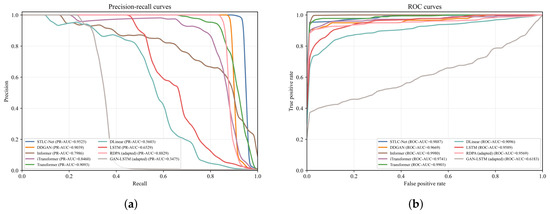
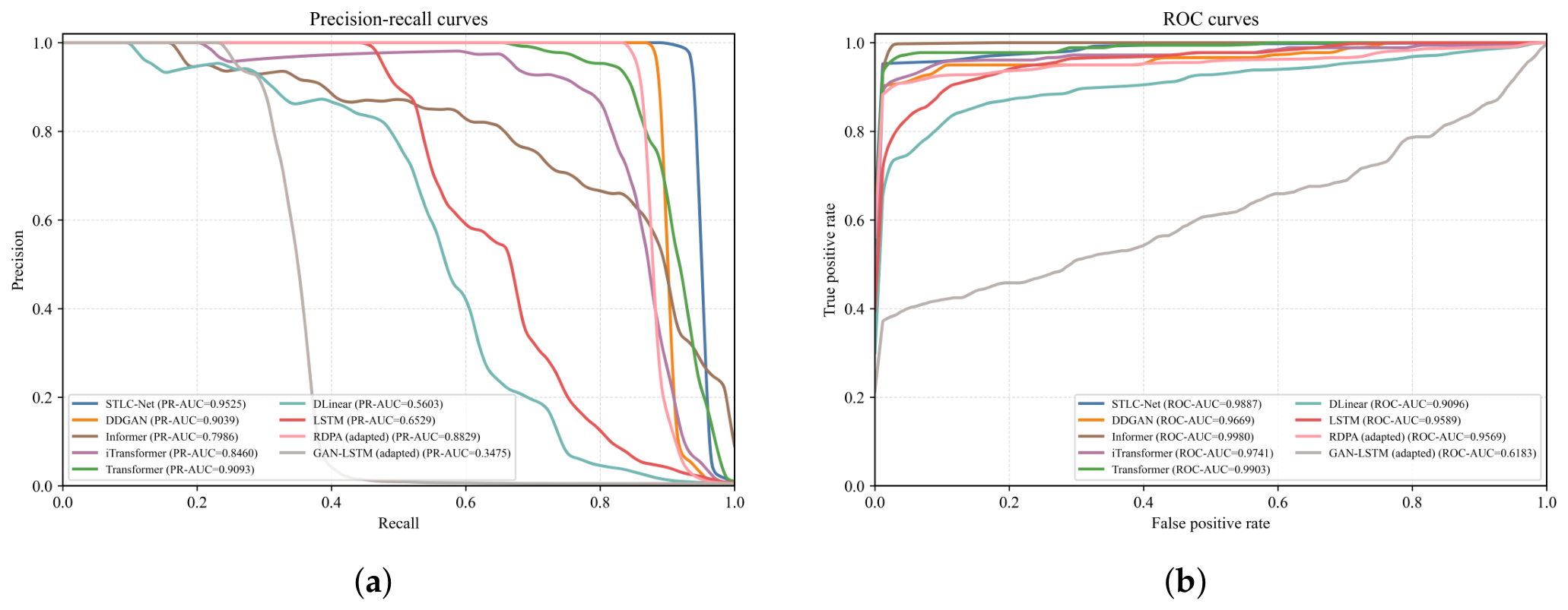
As shown in Table 2, STLC-Net achieved the highest PR-AUC, recall, and F1-score, with values of 0.952540, 0.882682, and 0.937685, respectively. Informer obtained the highest ROC-AUC, and Transformer also achieved a slightly higher ROC-AUC than STLC-Net. However, their lower PR-AUC, recall, and F1-score indicate that a high ROC-AUC alone does not necessarily correspond to effective detection of the rare anomalous class in the present highly imbalanced dataset.
Table 2.
Performance comparison of STLC-Net and baseline models under the unified window-level evaluation protocol.
Among the ADS-B-oriented baselines, RDPA achieved a PR-AUC of 0.882928 and an F1-score of 0.794613, whereas GAN-LSTM obtained a PR-AUC of 0.347511 and an F1-score of 0.311321. Under the same evaluation protocol, STLC-Net provided higher PR-AUC, recall, and F1-score than both adapted methods. These results suggest that the combination of short-window temporal modeling and latent-consistency scoring is suitable for detecting the local kinematic anomalies considered in this study.
Several models obtained a precision of 1.000000 under their validation-selected thresholds. This value indicates that no normal test windows were classified as anomalous at the corresponding operating points, but it does not imply complete anomaly detection. For example, DDGAN achieved a precision of 1.000000 but detected only 59.78% of the anomalous windows. STLC-Net retained a higher recall of 0.882682 while maintaining the same precision, resulting in a higher F1-score. The anomaly-score distributions of STLC-Net and DDGAN are examined further in Section 4.9.
Figure 2 presents the precision–recall and receiver operating characteristic curves of the compared models. Under the highly imbalanced setting considered in this study, the precision–recall curves provide a more direct assessment of the models’ ability to identify the rare anomalous class.
Figure 2.
PR and ROC curves of representative models. (a) Precision–recall curves. (b) ROC curves.
4.4. Model Component and Adversarial Regularization Ablation
To examine the respective contributions of temporal modeling, latent-consistency learning, and adversarial regularization, five model variants were evaluated. The LSTM reconstruction baseline retains the recurrent encoder–decoder structure but removes the secondary encoder and uses only reconstruction discrepancy for anomaly scoring. The non-recurrent GANomaly-style model retains the encoder–decoder–encoder latent-consistency structure but replaces the recurrent modules with non-recurrent mappings over the flattened trajectory window. Two additional variants introduce adversarial regularization into STLC-Net with and , respectively. The final STLC-Net combines recurrent temporal modeling with reconstruction and latent-consistency objectives, without adversarial regularization. All other data-processing, training, and evaluation settings were kept consistent across the variants.
As shown in Table 3, the LSTM reconstruction baseline obtained a PR-AUC of 0.652937 and an F1-score of 0.476596. After the secondary encoder and latent-consistency criterion were introduced, STLC-Net achieved a PR-AUC of 0.952540 and an F1-score of 0.937685. Because both models retain recurrent temporal modeling, this comparison indicates that reconstruction discrepancy alone is insufficient for the present task and that latent-consistency learning provides an important additional criterion for identifying abnormal trajectory windows.
Table 3.
Ablation results for model components and adversarial regularization.
The non-recurrent GANomaly-style model achieved the highest ROC-AUC and a PR-AUC close to that of STLC-Net, indicating that the encoder–decoder–encoder latent-consistency structure already provides strong anomaly-ranking capability. However, its recall and F1-score were 0.636872 and 0.778157, respectively, which were lower than the corresponding values of 0.882682 and 0.937685 obtained by STLC-Net. This comparison suggests that preserving the temporal order of consecutive ADS-B observations is beneficial for detecting a larger proportion of short-window kinematic anomalies at the selected operating threshold.
Introducing adversarial regularization did not further improve the results. With , the PR-AUC and F1-score decreased to 0.926140 and 0.895706. Increasing the adversarial weight to 0.005 further reduced the recall and F1-score to 0.642458 and 0.782313. These results indicate that the adversarial objective does not provide complementary benefits to reconstruction and latent-consistency learning under the present experimental setting. Therefore, adversarial regularization is excluded from the final STLC-Net training objective.
Overall, the ablation results distinguish the roles of the principal model components. Latent-consistency learning provides the main improvement over the reconstruction-only LSTM baseline, while recurrent temporal modeling improves anomaly coverage relative to the non-recurrent latent-consistency structure. In contrast, adversarial regularization is not required for the final model.
4.5. Effect of Window Size
To examine the influence of temporal context length, two datasets with window sizes of 16 and 32 were independently generated from the original flight trajectories. Both settings used the same flight-level split, stride of four, and 24-dimensional feature representation. For each window size, data standardization parameters and rule-labeling statistics were estimated separately from the corresponding training set. Therefore, the window-size-16 dataset was not obtained by cropping the window-size-32 dataset.
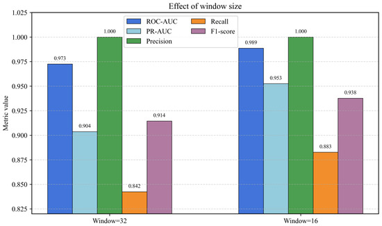
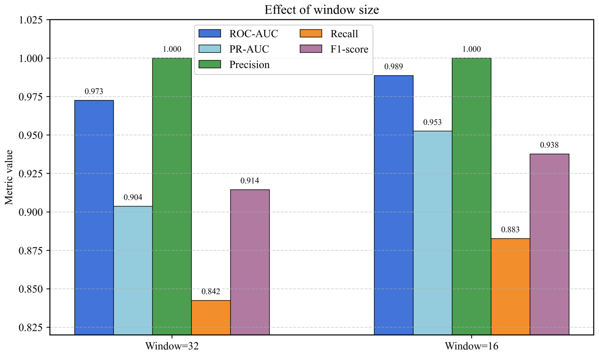
As shown in Figure 3, the window-size-16 setting achieved higher ROC-AUC, PR-AUC, recall, and F1-score than the window-size-32 setting, while both settings obtained a precision of 1.000000. In particular, reducing the window size from 32 to 16 increased PR-AUC from 0.903666 to 0.952540 and F1-score from 0.914454 to 0.937685.
Figure 3.
Effect of window size on the anomaly-detection performance of STLC-Net.
This result is consistent with the short-term characteristics of the rule-derived anomalies in the current dataset, which are mainly reflected by abrupt local speed discontinuities and unusually large first- or second-order motion variations. A longer window contains more surrounding normal observations and may weaken the relative contribution of a brief abnormal pattern, whereas a shorter window concentrates local trajectory changes within the input representation. Therefore, a window size of 16 was adopted as the default setting for the subsequent experiments.
4.6. Effect of Anomaly-Score Fusion
The final anomaly score of STLC-Net is obtained by combining the normalized reconstruction discrepancy and latent-space discrepancy with the fusion weight . To examine the influence of this parameter, was varied from 0.1 to 1.0, and the corresponding validation-set PR-AUC, F1-score, and recall were analyzed.
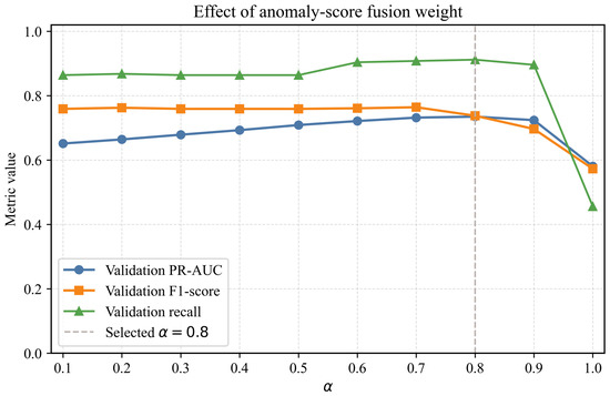
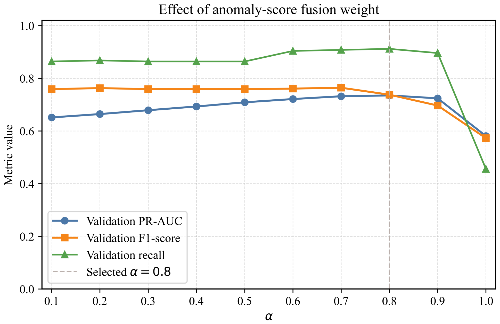
As shown in Figure 4, the validation PR-AUC increased steadily as increased from 0.1 to 0.8, indicating that assigning a larger weight to the reconstruction discrepancy improved the ranking quality of the anomaly scores. At the same time, the validation recall remained high over a broad range of values and reached its best level around , while the validation F1-score stayed relatively stable for intermediate values of and then declined when became too large.
Figure 4.
Effect of anomaly-score fusion weight on the validation performance of STLC-Net.
When approached 1.0, the contribution of latent-space discrepancy was substantially reduced, and all three validation metrics dropped noticeably, especially recall and F1-score. This result indicates that reconstruction discrepancy alone is insufficient for the present task and that latent-consistency information provides an important complementary cue. On the other hand, using too small an weakened the contribution of reconstruction discrepancy and led to lower PR-AUC.
Considering these trends together, was selected as the default setting for the subsequent experiments. This value provided the best overall trade-off among anomaly-score ranking quality, recall, and F1-score on the validation set, showing that a weighted combination of reconstruction discrepancy and latent-space discrepancy is more effective than relying on either component alone.
4.7. Stability Under Different Random Seeds
To examine the sensitivity of STLC-Net to random initialization and training-batch ordering, three independent experiments were conducted using random seeds 42, 52, and 62. The dataset split, pre-processing procedure, model architecture, and training hyperparameters were kept unchanged across all runs. Only the random seed controlling model initialization and the ordering of training batches was varied. The mean and sample standard deviation of the test metrics were then calculated across the three runs.
As shown in Table 4, STLC-Net maintained relatively consistent anomaly-ranking performance across the three independent runs. The standard deviations of ROC-AUC and PR-AUC were 0.007045 and 0.007199, respectively, while precision also remained stable with a standard deviation of 0.004511. These results indicate that the overall separation and ranking of normal and anomalous windows were not strongly dependent on a particular model initialization.
Table 4.
Performance of STLC-Net under different random seeds.
By comparison, recall and F1-score showed greater run-to-run variation, with standard deviations of 0.105161 and 0.066567, respectively. The main variation arose from the experiment with seed 52, which obtained a recall of 0.709497, compared with 0.882682 and 0.899441 for seeds 42 and 62. This difference indicates that threshold-dependent detection performance is more sensitive than threshold-independent ranking metrics to changes in model initialization and training-batch ordering under the highly imbalanced evaluation setting.
Across the three runs, STLC-Net achieved a mean PR-AUC of 0.947022 and a mean F1-score of 0.904035. The seed-42 result corresponds to the main experimental result reported in the preceding subsections, while the aggregated results provide a more comprehensive assessment of run-to-run stability. Overall, the repeated experiments support the consistency of the model’s anomaly-ranking capability, although the observed variation in recall and F1-score should be considered when interpreting performance at a fixed operating threshold.
4.8. Computational Efficiency
To assess the computational overhead and real-time application potential of STLC-Net, the number of trainable parameters and single-window inference latency were measured. STLC-Net contains 656,728 trainable parameters, requiring approximately 2.505 MB under 32-bit floating-point storage. The saved model checkpoint occupies 2.512 MB. Each timing measurement covered the complete forward computation through the first encoder, reconstruction decoder, and second encoder, as well as the calculation of the reconstruction discrepancy, latent discrepancy, and final anomaly score.
As shown in Table 5, STLC-Net processed one trajectory window in 3.901 ms on a single-thread CPU and 1.753 ms on the GPU. These results show that the two encoding passes, reconstruction decoding, and anomaly-score calculation introduce only millisecond-level processing latency. Compared with the 1 Hz sampling interval of the ADS-B data, this computational overhead supports the feasibility of online window-level anomaly screening. The reported values represent model-side inference latency after a complete input window has been formed.
Table 5.
Single-window inference efficiency of STLC-Net.
4.9. Anomaly-Score Distribution Analysis
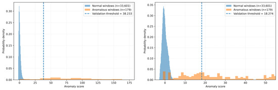
To provide a distribution-level assessment of anomaly detection performance, Figure 5 presents the test-set anomaly-score distributions of normal and anomalous windows for STLC-Net and DDGAN. The dashed lines indicate the decision thresholds selected from the corresponding validation sets.
Figure 5.
Anomaly-score distributions of normal and anomalous test windows for STLC-Net (left) and DDGAN (right). The dashed lines indicate the validation-selected thresholds.
STLC-Net produced a more concentrated normal-score distribution and a clearer shift of anomalous windows toward higher scores. Its KS statistic and overlap coefficient were 0.950099 and 0.057317, respectively, compared with 0.898429 and 0.121055 for DDGAN, indicating stronger class separation.
The DDGAN threshold of 18.273797 was selected using the same validation-based quantile procedure as the other models and was then fixed for test evaluation. At this operating point, no normal window exceeded the threshold, resulting in a precision of 1.000000. However, only 107 of the 179 anomalous windows were detected, yielding a recall of 0.597765. In comparison, STLC-Net detected 158 anomalous windows and achieved a recall of 0.882682. These results show that DDGAN generates relatively sparse high-confidence anomaly scores, whereas STLC-Net provides better anomaly coverage and stronger score separability.
4.10. External Multi-Regional Evaluation
To further assess the transferability of STLC-Net under changed sensing conditions, an additional ADS-B dataset provided by the Civil Aviation Flight University of China was used for external evaluation. The dataset contains 60 continuous trajectory segments collected from different regions using ADS-B receiving equipment different from that of the primary dataset. Following the same pre-processing and window-construction procedures, 21,926 trajectory windows were generated, including 218 rule-derived anomalous windows.
As shown in Table 6, STLC-Net achieved a ROC-AUC of 0.998484 and a PR-AUC of 0.869893 on the external dataset. Among the 218 rule-derived anomalous windows, 217 were detected, resulting in a recall of 0.995413. These results indicate that the model retained strong anomaly-score ranking and anomaly sensitivity under different regional and receiving conditions.
Table 6.
Performance of STLC-Net on the primary and external multi-regional ADS-B datasets.
In contrast, precision and F1-score decreased to 0.334361 and 0.500577, respectively. The lower precision indicates that more normal windows received scores above the fixed decision threshold when the model was applied to the external dataset. Therefore, although STLC-Net preserved strong ranking performance and detected nearly all rule-derived anomalies, its threshold-dependent performance was affected by the distributional differences between the two datasets.
5. Discussion
The experimental results indicate that the effectiveness of STLC-Net primarily arises from the combination of short-window temporal modeling and latent-consistency learning. Short windows preserve local kinematic changes, while the recurrent encoder–decoder–encoder structure evaluates both trajectory reconstruction and representation consistency. The ablation results show that reconstruction-only temporal modeling is insufficient, whereas the non-recurrent latent-consistency model provides strong anomaly ranking but lower anomaly coverage. Adversarial regularization does not yield additional benefits under the present setting. Therefore, the principal contribution of STLC-Net lies in integrating sequential modeling with reconstruction and latent-space discrepancies rather than in adversarial training.
The results also highlight several considerations for operational use. Under the highly imbalanced test setting, STLC-Net provides strong precision–recall performance and clearer separation between normal and anomalous scores than the compared generative baseline. Repeated training runs show relatively consistent ranking performance, although recall and F1-score remain more sensitive to random initialization and the validation-selected threshold. The external multi-regional evaluation preserves strong anomaly ranking and sensitivity, but the decrease in precision indicates that a fixed threshold can be affected by changes in receiver and data distributions. No false-positive windows were observed in the primary test set; however, the highest-scoring normal windows contained relatively pronounced but rule-consistent kinematic variations, suggesting that legitimate maneuvers may become potential false-alarm candidates under more sensitive thresholds or shifted operating conditions. The compact model size and millisecond-level inference latency support the computational feasibility of online window-level screening.
Several limitations should be considered. First, the rule-derived labels represent statistically unusual kinematic patterns rather than manually verified equipment faults, operational events, or malicious attacks. STLC-Net should therefore be interpreted as an anomaly-screening method rather than a causal-classification or message-authentication system. Second, data augmentation was not adopted because the model is trained in a one-class setting and the available anomalous labels are rule-derived; oversampling or synthesizing these samples could amplify labeling uncertainty. Although augmentation and imbalance-aware learning have shown value in supervised aviation-safety, their application in the present setting requires more reliable anomaly categories. Third, the current short-window design mainly targets local kinematic discontinuities, while gradual, persistent, or context-dependent anomalies may require longer-term trajectory information.
6. Conclusions
This study proposes STLC-Net for window-level anomaly detection in real-world ADS-B trajectories. The model combines short-window recurrent temporal modeling with reconstruction and latent-consistency discrepancies to identify unusual local kinematic patterns. Under the validation-based threshold-selection protocol, STLC-Net achieved the highest PR-AUC and F1-score among the compared methods. The ablation results confirm the complementary roles of temporal modeling and latent-consistency learning, while showing that adversarial regularization is not required in the final model. Repeated experiments, anomaly-score analysis, and computational evaluation further support the consistency of its anomaly-ranking performance, the separability of normal and anomalous windows, and its computational feasibility for online screening.
The external multi-regional evaluation showed that STLC-Net retained strong anomaly-ranking capability and anomaly sensitivity under different regional and receiving conditions, although its threshold-dependent precision decreased under the changed data distribution. Since the reference labels represent rule-derived kinematic anomalies rather than verified fault or attack categories, the proposed method should be regarded as a first-stage trajectory anomaly-screening approach. Future work will incorporate expert-verified and attack-injection data, extend independent cross-airport and multi-source evaluations, and investigate multi-scale temporal modeling, environment-specific threshold calibration, and finer-grained anomaly localization and cause identification.
Author Contributions
Conceptualization, X.L.; methodology, X.L.; validation, X.L. and L.Z.; formal analysis, L.Z.; investigation, K.X.; resources, K.X. and W.P.; data curation, X.L. and L.Z.; writing—original draft preparation, X.L.; writing—review and editing, L.Z., X.L. and K.X.; visualization, X.L.; supervision, K.X.; project administration, K.X. and W.P.; funding acquisition, W.P. All authors have read and agreed to the published version of the manuscript.
Funding
This research was supported by the Sichuan Science and Technology Program (2025YFHZ0023), the Henan Province Science and Technology Research Project (262102210224), the National Natural Science Foundation of China (U2333207), the Fundamental Research Funds for the Central Universities (26CAFUC01004, 26CAFUC04041), and the Open Fund Support from the Sichuan Provincial Engineering Research Centre for Flight and Operational Support of Domestic Civil Aircraft (MJCYZY202503).
Data Availability Statement
The datasets generated and analyzed during the current study are not publicly available due to confidentiality agreements and aviation data-sharing restrictions. Data may be made available from the corresponding author upon reasonable request and subject to appropriate permission.
Conflicts of Interest
Author Linfeng Zhong was employed by Luoyang Beijiao Airport Co., Ltd. The remaining authors declare that the research was conducted in the absence of any commercial or financial relationships that could be construed as a potential conflict of interest.
References
- Strohmeier, M.; Lenders, V.; Martinovic, I. On the security of the automatic dependent surveillance-broadcast protocol. IEEE Commun. Surv. Tutor. 2015, 17, 1066–1087. [Google Scholar] [CrossRef] [Scilit]
- Cevik, N.; Akleylek, S. Anomaly Detection System for ADS-B Data: Attack Vectors and Machine Learning Models. Internet Things 2025, 29, 101416. [Google Scholar] [CrossRef] [Scilit]
- Habler, E.; Shabtai, A. Using LSTM encoder-decoder algorithm for detecting anomalous ADS-B messages. Comput. Secur. 2018, 78, 155–173. [Google Scholar] [CrossRef] [Scilit]
- Fried, A.; Last, M. Facing airborne attacks on ADS-B data with autoencoders. Comput. Secur. 2021, 109, 102405. [Google Scholar] [CrossRef] [Scilit]
- Ying, X.; Mazer, J.; Bernieri, G.; Conti, M.; Bushnell, L.; Poovendran, R. Detecting ADS-B Spoofing Attacks Using Deep Neural Networks. In Proceedings of the 2019 IEEE Conference on Communications and Network Security (CNS), Washington, DC, USA, 10–12 June 2019; pp. 187–195. [Google Scholar]
- Karam, R.; Salomon, M.; Couturier, R. Supervised ADS-B Anomaly Detection Using a False Data Generator. In Proceedings of the 2022 2nd International Conference on Computer, Control and Robotics (ICCCR), Shanghai, China, 18–20 March 2022; pp. 218–223. [Google Scholar]
- Yue, M.; Zheng, H.; Cui, H.; Wu, Z. GAN-LSTM-Based ADS-B Attack Detection in the Context of Air Traffic Control. IEEE Internet Things J. 2023, 10, 12651–12665. [Google Scholar] [CrossRef] [Scilit]
- Zhong, L.; Liu, X.; Hao, Y.; Zhong, Q.; Huang, J.; Wu, T.; Pan, W.; Xu, K.; Shang, M. RDPA: Dual-domain deep learning for robust ADS-B spoofing detection via reversible normalization and spectral patch attention. Chin. J. Aeronaut. 2026, 104083. [Google Scholar] [CrossRef] [Scilit]
- Chandola, V.; Banerjee, A.; Kumar, V. Anomaly Detection: A Survey. ACM Comput. Surv. 2009, 41, 15. [Google Scholar] [CrossRef] [Scilit]
- Blazquez-Garcia, A.; Conde, A.; Mori, U.; Lozano, J.A. A Review on Outlier/Anomaly Detection in Time Series Data. ACM Comput. Surv. 2021, 54, 56. [Google Scholar] [CrossRef] [Scilit]
- Zamanzadeh Darban, Z.; Webb, G.I.; Pan, S.; Aggarwal, C.C.; Salehi, M. Deep Learning for Time Series Anomaly Detection: A Survey. ACM Comput. Surv. 2024, 57, 15. [Google Scholar] [CrossRef] [Scilit]
- Malhotra, P.; Ramakrishnan, A.; Anand, G.; Vig, L.; Agarwal, P.; Shroff, G. LSTM-Based Encoder-Decoder for Multi-Sensor Anomaly Detection. In Proceedings of the ICML 2016 Anomaly Detection Workshop, New York, NY, USA, 24 June 2016. [Google Scholar]
- Hundman, K.; Constantinou, V.; Laporte, C.; Colwell, I.; Soderstrom, T. Detecting Spacecraft Anomalies Using LSTMs and Nonparametric Dynamic Thresholding. In Proceedings of the 24th ACM SIGKDD International Conference on Knowledge Discovery and Data Mining, London, UK, 19–23 August 2018; pp. 387–395. [Google Scholar]
- Su, Y.; Zhao, Y.; Niu, C.; Liu, R.; Sun, W.; Pei, D. Robust Anomaly Detection for Multivariate Time Series through Stochastic Recurrent Neural Network. In Proceedings of the 25th ACM SIGKDD International Conference on Knowledge Discovery and Data Mining, Anchorage, AK, USA, 4–8 August 2019; pp. 2828–2837. [Google Scholar]
- Zhang, C.; Song, D.; Chen, Y.; Feng, X.; Lumezanu, C.; Cheng, W.; Ni, J.; Zong, B.; Chen, H.; Chawla, N.V. A Deep Neural Network for Unsupervised Anomaly Detection and Diagnosis in Multivariate Time Series Data. Proc. AAAI Conf. Artif. Intell. 2019, 33, 1409–1416. [Google Scholar] [CrossRef] [Scilit]
- Audibert, J.; Michiardi, P.; Guyard, F.; Marti, S.; Zuluaga, M.A. USAD: UnSupervised Anomaly Detection on Multivariate Time Series. In Proceedings of the 26th ACM SIGKDD International Conference on Knowledge Discovery and Data Mining, San Diego, CA, USA, 23–27 August 2020; pp. 3395–3404. [Google Scholar]
- Akcay, S.; Atapour-Abarghouei, A.; Breckon, T.P. GANomaly: Semi-Supervised Anomaly Detection via Adversarial Training. In Computer Vision—ACCV 2018; Springer: Cham, Switzerland, 2019; pp. 622–637. [Google Scholar]
- Wang, J.; Zou, Y.; Ding, J. ADS-B spoofing attack detection method based on LSTM. EURASIP J. Wirel. Commun. Netw. 2020, 2020, 160. [Google Scholar] [CrossRef] [Scilit]
- Kacem, T.; Tossou, S. ADS-B replay attack detection using transformers. In Proceedings of the 2024 International Wireless Communications and Mobile Computing (IWCMC), Ayia Napa, Cyprus, 27–31 May 2024; pp. 144–149. [Google Scholar]
- Proud, S.R. Go-Around Detection Using Crowd-Sourced ADS-B Position Data. Aerospace 2020, 7, 16. [Google Scholar] [CrossRef] [Scilit]
- Kumar, S.G.; Corrado, S.J.; Puranik, T.G.; Mavris, D.N. Classification and Analysis of Go-Arounds in Commercial Aviation Using ADS-B Data. Aerospace 2021, 8, 291. [Google Scholar] [CrossRef] [Scilit]
- Matthews, B.; Nielsen, D.; Schade, J.; Chan, K.; Kiniry, M. Automated Discovery of Flight Track Anomalies. In Proceedings of the 2014 IEEE/AIAA 33rd Digital Avionics Systems Conference (DASC), Colorado Springs, CO, USA, 5–9 October 2014. [Google Scholar]
- Cao, Y.; Cao, J.; Zhou, Z.; Liu, Z. Aircraft Track Anomaly Detection Based on MOD-Bi-LSTM. Electronics 2021, 10, 1007. [Google Scholar] [CrossRef] [Scilit]
- Huang, T.; Wu, H.; Tao, X.; Wei, Z. Prediction-Based Trajectory Anomaly Detection in UAV System with GPS Spoofing Attack. Chin. J. Aeronaut. 2025, 38, 103478. [Google Scholar] [CrossRef] [Scilit]
- Li, L.; Hansman, R.J. Anomaly Detection in Airline Routine Operations Using Flight Data Recorder Data; Report No. ICAT-2013-4; MIT International Center for Air Transportation: Cambridge, MA, USA, 2013. [Google Scholar]
- Vaswani, A.; Shazeer, N.; Parmar, N.; Uszkoreit, J.; Jones, L.; Gomez, A.N.; Kaiser, L.; Polosukhin, I. Attention Is All You Need. In Advances in Neural Information Processing Systems; Curran Associates, Inc.: Red Hook, NY, USA, 2017; Volume 30. [Google Scholar]
- Xu, J.; Wu, H.; Wang, J.; Long, M. Anomaly Transformer: Time Series Anomaly Detection with Association Discrepancy. In Proceedings of the 10th International Conference on Learning Representations (ICLR), Virtual Event, 25–29 April 2022. [Google Scholar]
- Tuli, S.; Casale, G.; Jennings, N.R. TranAD: Deep Transformer Networks for Anomaly Detection in Multivariate Time Series Data. Proc. VLDB Endow. 2022, 15, 1201–1214. [Google Scholar]
- Ayhan, B.; Vargo, E.P.; Tang, H. On the Exploration of Temporal Fusion Transformers for Anomaly Detection with Multivariate Aviation Time-Series Data. Aerospace 2024, 11, 646. [Google Scholar] [CrossRef] [Scilit]
- Zhou, Y.; Fu, C.; Wei, L.; Zhou, W.; Li, X.; You, Y. An Integrated Approach for Addressing Data Imbalance in Predicting Fatality of Helicopter Accident. Reliab. Eng. Syst. Saf. 2026, 267, 111921. [Google Scholar] [CrossRef] [Scilit]
- Hou, Z.; Wang, H.; Xiong, M.; Liu, W. Highly Imbalanced Intelligent Identification of Civil Aviation Maintenance Hazards Based on Text Mining and Selective Ensemble Modeling. Eng. Appl. Artif. Intell. 2026, 173, 114403. [Google Scholar] [CrossRef] [Scilit]
- Zong, B.; Song, Q.; Min, M.R.; Cheng, W.; Lumezanu, C.; Cho, D.; Chen, H. Deep Autoencoding Gaussian Mixture Model for Unsupervised Anomaly Detection. In Proceedings of the 6th International Conference on Learning Representations (ICLR), Vancouver, BC, Canada, 30 April–3 May 2018. [Google Scholar]
- Xu, H.; Chen, W.; Zhao, N.; Li, Z.; Bu, J.; Li, Z.; Liu, Y.; Zhao, Y.; Pei, D.; Feng, Y.; et al. Unsupervised Anomaly Detection via Variational Auto-Encoder for Seasonal KPIs in Web Applications. In Proceedings of the 2018 World Wide Web Conference, Lyon, France, 23–27 April 2018; pp. 187–196. [Google Scholar]
- Zhu, G.; Zhao, H.; Liu, H.; Sun, H. A Novel LSTM-GAN Algorithm for Time Series Anomaly Detection. In Proceedings of the 2019 Prognostics and System Health Management Conference (PHM-Qingdao), Qingdao, China, 25–27 October 2019; pp. 1–6. [Google Scholar]
- Li, D.; Chen, D.; Shi, L.; Jin, B.; Goh, J.; Ng, S.-K. MAD-GAN: Multivariate Anomaly Detection for Time Series Data with Generative Adversarial Networks. In Artificial Neural Networks and Machine Learning—ICANN 2019: Text and Time Series; Springer: Cham, Switzerland, 2019; pp. 703–716. [Google Scholar]
- Geiger, A.; Liu, D.; Alnegheimish, S.; Cuesta-Infante, A.; Veeramachaneni, K. TadGAN: Time Series Anomaly Detection Using Generative Adversarial Networks. In Proceedings of the 2020 IEEE International Conference on Big Data (Big Data), Atlanta, GA, USA, 10–13 December 2020; pp. 33–43. [Google Scholar]
- Bashar, M.A.; Nayak, R. ALGAN: Time Series Anomaly Detection with Adjusted-LSTM GAN. Int. J. Data Sci. Anal. 2025, 20, 5719–5737. [Google Scholar] [CrossRef] [Scilit]
- Sokolova, M.; Lapalme, G. A systematic analysis of performance measures for classification tasks. Inf. Process. Manag. 2009, 45, 427–437. [Google Scholar] [CrossRef] [Scilit]
- Zeng, A.; Chen, M.; Zhang, L.; Xu, Q. Are Transformers Effective for Time Series Forecasting? Proc. AAAI Conf. Artif. Intell. 2023, 37, 11121–11128. [Google Scholar] [CrossRef] [Scilit]
- Liu, Y.; Hu, T.; Zhang, H.; Wu, H.; Wang, S.; Ma, L.; Long, M. iTransformer: Inverted Transformers Are Effective for Time Series Forecasting. In Proceedings of the 12th International Conference on Learning Representations (ICLR), Vienna, Austria, 7–11 May 2024. [Google Scholar]
- Zhou, H.; Zhang, S.; Peng, J.; Zhang, S.; Li, J.; Xiong, H.; Zhang, W. Informer: Beyond Efficient Transformer for Long Sequence Time-Series Forecasting. Proc. AAAI Conf. Artif. Intell. 2021, 35, 11106–11115. [Google Scholar] [CrossRef] [Scilit]
- Ding, D.; Wang, Y.; Tao, H.; Wu, J.; Cao, J. A Dual-Discriminator Generative Adversarial Network for Anomaly Detection. IEEE Trans. Neural Netw. Learn. Syst. 2025, 36, 19285–19296. [Google Scholar] [CrossRef] [Scilit] [PubMed]

Disclaimer/Publisher’s Note: The statements, opinions and data contained in all publications are solely those of the individual author(s) and contributor(s) and not of MDPI and/or the editor(s). MDPI and/or the editor(s) disclaim responsibility for any injury to people or property resulting from any ideas, methods, instructions or products referred to in the content. |
© 2026 by the authors. Licensee MDPI, Basel, Switzerland. This article is an open access article distributed under the terms and conditions of the Creative Commons Attribution (CC BY) license.