Numerical Simulation Method for Fluid–Structure Interaction of Deformable Structures Based on Multibody Dynamics

Abstract

With the development of morphing aircraft, understanding the fluid–structure interaction (FSI) mechanisms of multibody systems composed of rigid and flexible components has become increasingly important. The coupled motion and deformation of such systems in a flow field give rise to complex nonlinear FSI problems. Here, we propose a fluid–multibody–structure interaction framework that couples a finite volume Navier–Stokes solver, a multibody dynamics solver, and radial basis function interpolation for fluid–structure data transfer. The framework is validated using a benchmark case and subsequently applied to simulations of a two-segment flexible beam and a three-dimensional continuously variable-sweep wing. The results show that the presence of joints and structural flexibility substantially affects the FSI response: hinge location markedly alters the FSI characteristics of the multibody flexible-beam system, while increasing the sweep angle during continuous morphing reduces the aerodynamic force coefficients and structural flexibility induces persistent fluctuations in aerodynamic loads. A key contribution of the proposed framework is its ability to capture both active morphing motions and passive aeroelastic deformations simultaneously. Compared with approaches based on inviscid, incompressible aerodynamic models, the present high-fidelity flow solver can better resolve complex flow phenomena during morphing. This framework provides a useful numerical tool for investigating FSI mechanisms in morphing aircraft. Its current limitations include the computational cost of global radial basis function interpolation for large multibody systems and its applicability being restricted to low-Mach-number flows.

1. Introduction

Learning from nature is the source of innovation for human beings to develop technologies that improve the efficiency, mobility and environmental adaptability of bionic machines. Understanding the movement mechanism of organisms and revealing the interaction mechanism between them and the environment is the constant pursuit of scientific research and an important way to design more efficient bionic machines [1,2,3]. Inspired by biology, in-flight morphing aircraft are becoming a key means to address the aerodynamic trade-offs between different flight performance requirements [4,5,6,7,8,9,10].

The most significant difference between flexible multibody morphing wing surfaces and conventional fixed-configuration aircraft wings lies in the presence of kinematic constraints among multiple wing components connected through joints, which enable various morphing modes, including bending, twisting, extension, and their combinations [11,12,13,14,15,16,17,18,19]. At this point, wings are no longer considered single-body structures but rather a multibody system [20,21,22,23,24]. Research on such multibody systems will contribute to the development of morphing aircraft and new biomimetic machines. A multibody system consists of multiple rigid or flexible bodies connected to each other through joints. Such systems are widespread in nature; for example, bat wings can be viewed as comprising a skeleton and flexible membranes connected by joints, allowing for up to 40 additional degrees of freedom in wing kinematics [25]. The presence of these joints constrains movement patterns and increases movement complexity. These new insights into the mechanisms of bat flight underscore the importance of not neglecting fluid–structure interaction effects—including the dynamic characteristics of actuation mechanisms—when designing flexible morphing wings, as such effects can have a significant impact on flight performance.

Deformations of multibody wing surfaces within a flow field can be either active or passive, resulting in a highly nonlinear problem that involves the coupling of fluid motion equations with body movement equations. The presence of these joints significantly amplifies the kinematic complexity of the structure, leading to various fluid–structure coupling phenomena and mechanisms. Therefore, establishing a numerical simulation method for fluid–structure interaction targeting multibody systems is an important and meaningful endeavor. Currently, fluid–structure interaction numerical simulations for such multibody systems remain scarce. An in-depth understanding of the complex interaction mechanism between multibody structures and unsteady flow fields is a common key scientific issue faced in revealing the secret of efficient propulsion of the wings of flying and wandering organisms and designing high-performance flexible bionic aircraft.

The classical aeroelastic approach treats the wing as a single flexible structure, analyzed through fluid–structure coupling frameworks based on modal methods or finite element formulations. For instance, Xue et al. [26] investigated the effects of structural geometric nonlinearities on the transonic aeroelastic characteristics of wings, demonstrating the importance of large-deformation modeling for accurately predicting flutter boundaries. Grifò and Ronch [27] established a unified computational aeroelastic framework that integrates high-order structural models with high-fidelity aerodynamics. Zhang et al. [28] performed geometrically nonlinear flutter analysis based on CFD-CSD coupling with wind tunnel validation. Wang et al. [29] and Yang et al. [30] addressed large-deformation static aeroelasticity and reduced-order modeling for high-aspect-ratio wings. While these methods provide high-fidelity deformation prediction with well-established accuracy, they are fundamentally incapable of handling joint kinematics in multibody morphing configurations. Moreover, their computational cost is considerably higher than that of rigid-body approaches—a trade-off that motivates the adoption of simplified treatments for configurations where joint kinematics dominates over structural deformation.

A computationally leaner alternative is to simplify the morphing wing into a system of multiple rigid bodies connected by joints. For example, Eldredge [31] simulated the simplified undulation motion of an anguilliform free-swimming fish by prescribing the motion forms of three two-dimensional rigid bodies. Wang et al. [32] investigated a bionic dual-joint flapping wing with local swept variation, consisting of inner and outer sections that unfold about the shoulder and wrist joints, respectively. These studies are tailored to specific configurations, each requiring the derivation of a dedicated set of governing equations, which must be rederived when the object of investigation changes and are therefore not readily generalizable. Coupling multibody dynamics with a flow solver can achieve better generality. For instance, Li et al. [33] combined a multibody tree-like solution algorithm with the user-defined function of ANSYS Fluent to develop a multi-rigid-body FSI method for fish swimming simulation. Le et al. [34] proposed a multibody dynamics approach for moth-like flapping wings, discretizing the wing into a chain of rigid bodies connected by springs and coupling the structural dynamics with an unsteady vortex lattice method. However, by neglecting structural flexibility entirely, these approaches cannot capture the influence of elastic deformation on aerodynamic load distribution, which may lead to inaccurate predictions of load redistribution in configurations where flexibility plays a non-negligible role.

To overcome the constraints of single-body flexibility and multi-rigid-body simplification, recent efforts have sought to integrate flexible multibody dynamics algorithms with flow field solvers, thereby accommodating both structural deformation and joint kinematics within a single framework. Cheng et al. [35] coupled a multibody solver based on geometrically exact composite beams with an unsteady vortex lattice method (UVLM) for aeroelastic simulation of a flexible wing with a hinged wingtip. Han et al. [36] developed a multibody dynamics formulation coupled with UVLM for nonlinear aeroelastic response analysis of wings with flared folding wingtips, revealing that geometric nonlinearity significantly affects dynamic response during active wingtip folding. While these frameworks successfully resolve the joint kinematic limitation and capture structural flexibility, they rely on a UVLM as the aerodynamic model, which is inherently restricted to inviscid, attached-flow regimes and cannot resolve viscous effects and flow separation—phenomena that become significant during large-amplitude morphing motions. Joshi et al. [37] addressed the FSI problem of bat-inspired multibody flapping wings by coupling a variational flexible multibody formulation with an incompressible finite element flow solver for application to bat-like unmanned aerial vehicles. In summary, existing efforts that incorporate flexible multibody dynamics within an FSI framework are still limited in scope. The available methods typically adopt inviscid, incompressible aerodynamic models that restrict their fidelity in complex flow conditions. The simultaneous representation of actively driven morphing and passively induced aeroelastic deformation of morphing wings thus remains a challenge.

In this paper, the finite volume method flow field solver is combined with a general multibody structure dynamics solver to simulate the fluid–structure coupling of flexible multibody structures. By studying the coupling effect between fluid and flexible multibody structures, the coupling mechanism is further revealed. The fluid solver used is a finite volume solver that solves the three-dimensional Navier–Stokes (N-S) equations. The solver is capable of simulating compressible viscous flows. A multibody dynamic code MBDyn was used to solve the multibody dynamics, and the radial basis function (RBF) method was developed to carry out data mapping on the fluid–structure interface. The moving mesh method was applied to achieve flow grid adaption according to the deformation of the structures. The primary advantage of the proposed framework is its ability to simultaneously capture joint-actuated active continuous morphing and the passive aeroelastic deformation of flexible wing components under unsteady aerodynamic loads within a unified high-fidelity coupled simulation framework. The accuracy of the proposed method is verified by fluid structure interaction benchmark examples. Subsequently, the proposed method is applied to the numerical simulation of a multibody system consisting of two flexible beams connected by rotational hinges, as well as a three-dimensional rotating variable-sweep wing.

The article is organized as follows: in Section 2, the numerical method is introduced; in Section 3, the accuracy and feasibility of this method are validated through a benchmark example of fluid–structure interaction; in Section 4, a multibody system consisting of two flexible beams connected by a revolute hinge is constructed, and numerical simulations of fluid–structure interaction are conducted on it; in Section 5, numerical simulation of a continuously variable-sweep wing is conducted. The main conclusions are given in Section 6.

2. Introduction of Numerical Framework

In this section, the proposed FSI numerical framework including the fluid dynamics solution method, the multibody dynamics solution method, and the data exchange method and coupling strategy between the fluid interface and the multibody interface is described.

2.1. Fluid Dynamics Solution

Flow motion follows three conservation laws, namely, the law of conservation of mass, momentum and energy. The three conservation laws constitute the fundamental equations of fluid mechanics. The general form of the governing equation can be expressed by the following equation:

$${\displaystyle \frac{\partial \left(\rho \varphi \right)}{\partial t}}+\nabla \cdot \left(\rho U\varphi \right)=\nabla \cdot \left({\mathsf{\Gamma }}_{\varphi }\nabla \varphi \right)+S_{\varphi },$$

(1)

In the formula, $\varphi$ is a universal variable, which can represent solving variables. ${\mathsf{\Gamma }}_{\varphi }$ is the generalized diffusion coefficient, and $S_{\varphi }$ is the generalized source term. Under the continuum assumption and neglecting body forces and external heat sources, the three-dimensional unsteady compressible Navier–Stokes equations in a Cartesian coordinate system can be written in differential form as follows.

The conservation of mass is given by the following:

$${\displaystyle \frac{\partial \rho }{\partial t}}+\nabla \cdot (\rho U)=0,$$

(2)

While the conservation of momentum reads as follows:

$${\displaystyle \frac{\partial \left(\rho U\right)}{\partial t}}+\nabla \cdot (\rho UU)=-\nabla p+\nabla \cdot \tau ,$$

(3)

where ρ is the density, $U=\left(u,v,w\right)$ is the velocity vector, and $p$ denotes the pressure. The total energy equation is expressed as

$${\displaystyle \frac{\partial \left(\rho E\right)}{\partial t}}+\nabla \cdot \left[\begin{array}{c}(\rho E+p)U\end{array}\right]=\nabla \cdot (\tau \cdot U)-\nabla \cdot q,$$

(4)

with $E=e+{\displaystyle \frac{1}{2}}{\left|U\right|}^2$ being the total energy per unit mass. For a Newtonian fluid, the viscous stress tensor $\tau$ is defined as

$$\tau =\mu \left(\nabla U+\nabla U^T\right)-{\displaystyle \frac{2}{3}}\mu (\nabla \cdot U)\mathrm{I}.$$

(5)

And the heat flux vector is modeled by Fourier’s law $q=-k\nabla T$. The system is closed by the ideal gas equation of state $p=\rho RT$.

The finite volume method (FVM) was used to solve the N-S equations. It is capable of simulating both steady and unsteady flows, as well as compressible and incompressible flows. Turbulence effects are modeled using the $k$ - $\omega sst$ turbulence model. The discretization scheme for the convective terms is critical in solving the N-S equations. While the diffusive terms are generally discretized using a central-difference scheme, several schemes can be adopted for the convective terms. Here, the second-order upwind scheme was employed to discretize the convective terms.

2.2. Multibody Dynamics Solution

2.2.1. Fundamental Equations

MBDyn (Version 1.7.3) is a general multibody dynamics analysis software, which was developed by the Institute of Aeronautical Science and Technology, Polytechnic University of Milan, Italy. The program uses Lagrange multipliers or redundant coordinate set formulations for systems where multiple rigid or flexible bodies are connected by kinematic constraints. For each member of the constrained system, the Newton–Euler equations of motion are established in differential algebraic form, and the first-order equations are established together with the constraint equations [38].

The fundamental equations behind the structural dynamics implemented in MBDyn software consist of Newton–Euler equations. The equations for each body are expressed as follows:

$$m\dot{x}=\beta ,$$

(6)

$$J\omega +S\times \dot{x}=\gamma ,$$

(7)

In the above equations, $\beta$ and $\gamma$ represent the linear and angular momenta; $m$ is the mass; $\dot{x}$ is the velocity; $S$ is the first moment of inertia; $J$ is the second moment of inertia; $\omega$ is the angular velocity. Each structural node used in the simulation model is linked to its own equation for $\beta$ and $\gamma$.

The equilibrium equations are established as follows:

$$\dot{\beta }=p,$$

(8)

$$\dot{\gamma }+\dot{x}\times \beta =q,$$

(9)

where $\ddot{x}$ is the acceleration vector, and $p$ and $q$ represent force and torque, respectively.

2.2.2. Constrained Equations

The boundary conditions and constraints are realized by adding constraints to the equations, which can be holonomic or nonholonomic, and these constraints are realized by using Lagrange multipliers. For the analysis of the execution initial value problem (IVP), whether static or dynamic, the expression of the constraint mechanics IVP is as follows:

$$M\dot{x}-\mathsf{\alpha }=0,$$

(10)

$$\dot{\alpha }+{\varphi }_{,x}^T{\lambda }_{\varphi }+{\psi }_{,\dot{x}}^T{\lambda }_{\psi }-f\left(x,\dot{x},t\right)=0,$$

(11)

$$\varphi \left(x,t\right)=0,$$

(12)

$$\psi \left(x,\dot{x},t\right)=0,$$

(13)

where $M$ denotes the inertia matrix of the body; $\mathsf{\alpha }$ is the momentum of the body, referring to the whole rigid-body momentum definition; $x$ represents the vector of the generalized coordinates including both translational and rotational parameters; $f$ denotes the generalized forces and moments, which may depend on the configuration. ${\lambda }_{\varphi }$ and ${\lambda }_{\psi }$ are Lagrange multipliers associated with holonomic and nonholonomic constraint equations ${\varphi }_{,x}^T$ is the transpose of the partial derivative of the holonomic constraint $\varphi$ with respect to $x$; ${\psi }_{,\dot{x}}^T$ is the transpose of the partial derivative of the nonholonomic constraint $\psi$ with respect to $\dot{x}$.

2.2.3. Time Integration

The above generalized dynamic problem can be formulated as the following differential algebraic system (DAE):

$$r\left(x,\dot{x},t\right)=0$$

(14)

An implicit A/L-stable linear multistep integration scheme is used for time integration of the above equation,

$$x_k={\sum }_{i=\mathrm{1,2}}{a}_i{x}_{k-i}+h{\sum }_{i=\mathrm{0,2}}{b}_i{\dot{x}}_{k-i},$$

(15)

where $a$ and $b$represent the coefficients of the format used, and $h$ is the time step.

The coefficients are chosen in the following form:

$$a_1=1-\beta , a_2=\beta ,$$

(16)

$$b_0=\delta /\alpha +\alpha /2,$$

(17)

$$b_1=\beta /2+\alpha /2-(1+\alpha )\delta /\alpha ,$$

(18)

$$b_2=\beta /2+\delta ,$$

(19)

With

$$\begin{array}{c}\alpha =(t_k-t_{k-1})/(t_{k-1}-t_{k-2})\\ \beta =\alpha {\displaystyle \frac{(2+\alpha )(1-|{\rho }_{\mathrm{\infty }}|{)}^2+2(1+\alpha \left)\right(2\left|{\rho }_{\mathrm{\infty }}\right|-1)}{2(1+\alpha )-(1-|{\rho }_{\mathrm{\infty }}|{)}^2}}\\ \delta ={\displaystyle \frac{{\alpha }^2(1-|{\rho }_{\mathrm{\infty }}|{)}^2}{2\left(2\right(1+\alpha )-(1-\left|{\rho }_{\mathrm{\infty }}\right|{)}^2)}}\end{array},$$

(20)

A-stability (unconditional stability) is obtained by choosing $0\le \left|{\rho }_{\mathrm{\infty }}\right|\le 1$. The above coefficients are chosen to ensure the second-order accuracy and stability of the format, and at the same time the numerical dissipation can be adjusted; for a detailed description of the content of this part, please refer to the literature [38]. The prediction correction method is used to solve the above equation.

2.3. Coupling Interface Data Transfer

In the process of partition-based fluid–structure interaction calculation, the aerodynamic pressure of the fluid surface is calculated on the fluid grid, and the structural response is solved on the structural node. Usually, the two grids are inconsistent, so it is necessary to interpolate the physical quantity data between the two grids. The Radial basis function (RBF) interpolation method is used for data interaction. The RBF method can directly carry out data transmission of all discrete clouds, and only node coordinates are needed in the interpolation process, without the connection information between nodes. The Radial basis function (RBF) is an interpolation method widely used in fluid–structure interaction calculation, which can be used to obtain the interpolation relationship between displacements

Let us suppose that a set of spatial discrete points $X=\{x_1,x_2,\cdots ,x_N\}\subseteq R^d$ known in a d-dimensional Euclidean space is called the center point. A continuous function can be determined from the known discrete points so that the function passes through these central points. A continuous function is called an RBF interpolation function when it takes the form of the following equation:

$$s(x)={\displaystyle {\sum }_{i=1}^N} {\alpha }_i\varphi (\parallel x-x_i\parallel )+p(x),$$

(21)

where $s\left(x\right)$ is the unknown function value at point $x$; $x$ is the coordinates of unknown points; $x_i$ is the known coordinate of the center point.

The $\varphi$ function is an interpolation function. The common forms are as follows: Gaussian (G) and Thin Plate Spline (TPS). The TPS kernel function is given by $\varphi \left(r\right)=r^2\mathrm{l}\mathrm{n}\left(r\right)$ and does not require any additional parameters. The Gaussian kernel function is given by $\varphi \left(r\right)=e^{-{\left(\mathcal{E}r\right)}^2}$, in which $\mathcal{E}$ is the key parameter governing interpolation accuracy and numerical stability. This parameter is calculated as $\mathcal{E}=1/\left(2.5h\right)$, where $h$ denotes the mean nearest-neighbor distance between nodes on the interface.

${\alpha }_i$ is the coefficient corresponding to the center point; $\parallel x-x_i\parallel$ is the Euclidean space distance, expressed as follows:

$$r=\parallel x-x_i\parallel ={\left[{\left(x-x_i\right)}^2+{\left(y-y_i\right)}^2+{\left(z-z_i\right)}^2\right]}^{1/2},$$

(22)

$p\left(x\right)$ is a polynomial; a first-order linear polynomial can generally meet the requirements, expressed as follows:

$$p\left(x\right)={\gamma }_0+{\gamma }_{x}x+{\gamma }_{y}y+{\gamma }_{z}z,$$

(23)

The ${\alpha }_i$ coefficients and coefficients in the polynomial $p\left(x\right)$ are obtained according to the following definite solution conditions:

$$s\left(x_i\right)=g_{i}i=\mathrm{1,2},\cdots ,N,$$

(24)

$${\displaystyle {\sum }_{i=1}^N} {\alpha }_{i}q\left(x_i\right)=0,q\left(x\right)=1,x,y,z,$$

(25)

In the above formula, $x_i$ is the known data center point; $g_i$ is the known function value; $q\left(x\right)$ is a polynomial function, where the order of $q\left(x\right)$ meets $\mathrm{d}\mathrm{e}\mathrm{g}\left[q\right(x\left)\right]⩽\mathrm{d}\mathrm{e}\mathrm{g}\left[p\right(x\left)\right]$.

Let us suppose that on the fluid–structure interaction surface, there are $N_s$ and $N_f$ interpolation points in the solid domain and the fluid domain. By using the Radial basis function (RBF), the interpolation relationship between the displacements of the interface nodes is expressed in matrix form as follows:

$$\delta u_f=H·\delta u_s,$$

(26)

where $\delta u_f$ and $\delta u_s$ represent the displacement on the fluid grid node and the displacement on the structure node, and $H$ is the mapping matrix.

Using the principle of virtual work, the interpolation relationship between the aerodynamic force and the structural node force can be obtained by

$$\delta W=\delta u_s^T·f_s=\delta u_f^T·f_f.$$

(27)

The interpolated relationship between loads is obtained as follows:

$$f_s=H^T·f_f$$

(28)

2.4. Coupling Strategy

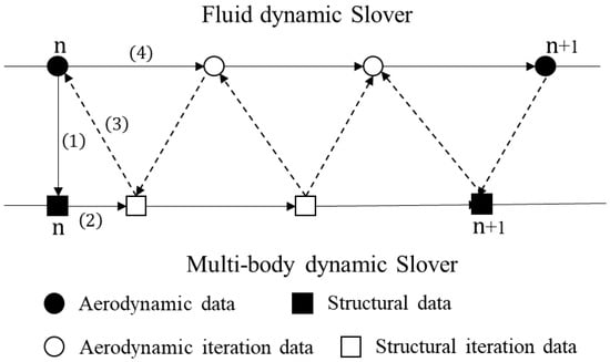
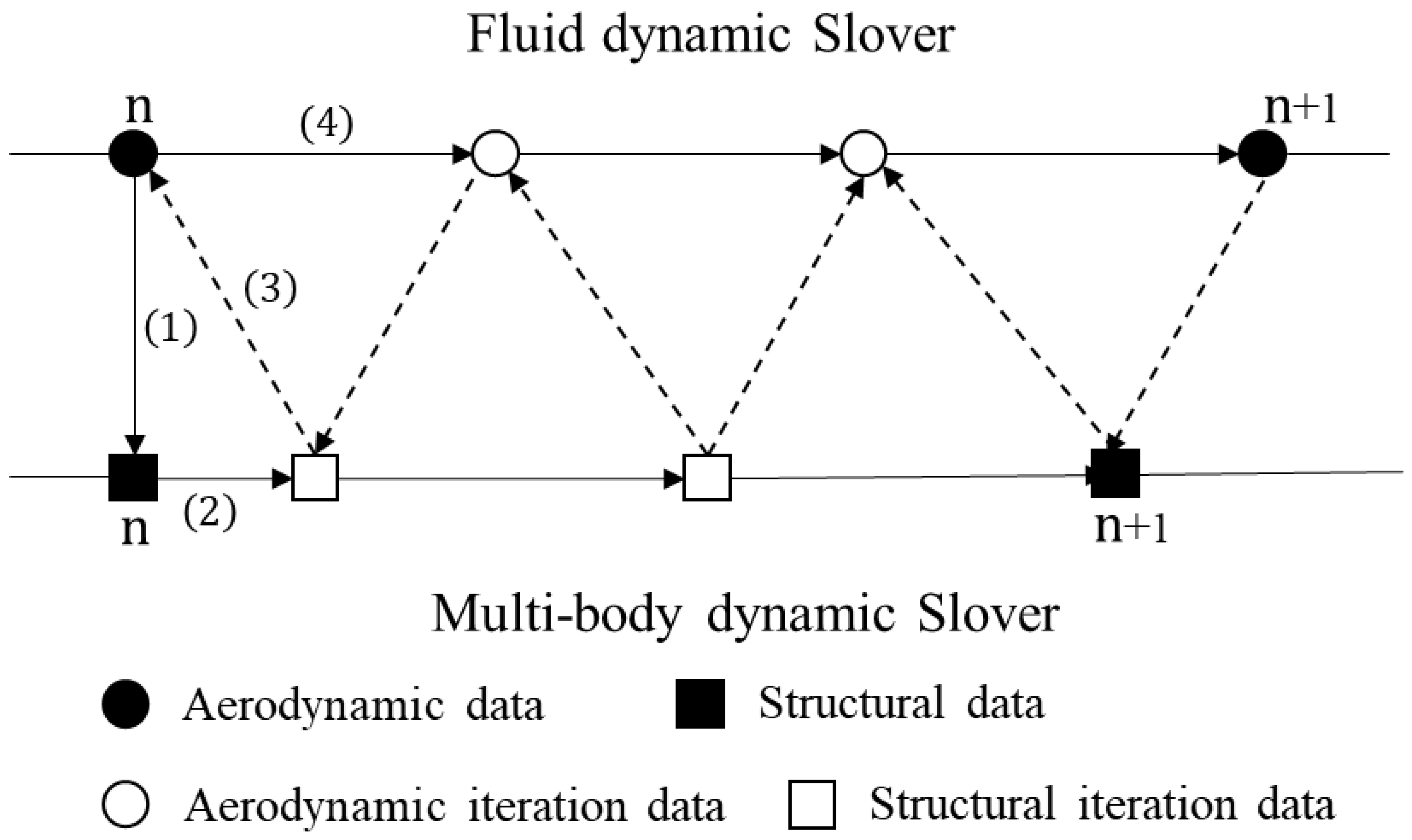
A tightly coupled strategy is adopted. The participants are coupled iteratively, repeating each coupling time window until both sides of the interface have converged. The detailed implementation process of tight coupling is shown in Figure 1:

Figure 1. Schematic diagram of coupling iteration.

(1)

The fluid force at time n is mapped to the structural node;

(2)

Solve the dynamics and advance to time n + 1/k (k is the number of sub-iteration steps);

(3)

Physical quantities such as displacement and velocity are mapped from structural nodes to fluid grids;

(4)

Perform mesh deformation to solve the flow force at time n + 1/k.

The k sub-iteration process is repeated until the fluid state at time n + 1 is obtained, and the current time step iteration calculation is completed. We cycle through the next time step until convergence conditions are reached.

Within each time step, force and displacement convergence criteria are imposed at the coupling interface, together with a maximum number of coupling iterations. The simulation advances to the next time step only after these convergence criteria are satisfied. Residual convergence criteria and maximum numbers of internal iterations are specified independently for the fluid and structural solvers.

3. Validation of the Numerical Framework

In this section, the benchmark test case for a single-body flexible-beam model proposed by Turek and Hron [39] is calculated to test the accuracy of the flow solver, structure solver and the FSI framework in this paper. The verification example used in this paper is a set of well-known benchmark tests in the FSI literature which have been numerically verified by many people. The structural model will be established via the multibody dynamics method and will be compared with the finite element method.

3.1. Problem Description

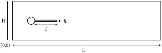
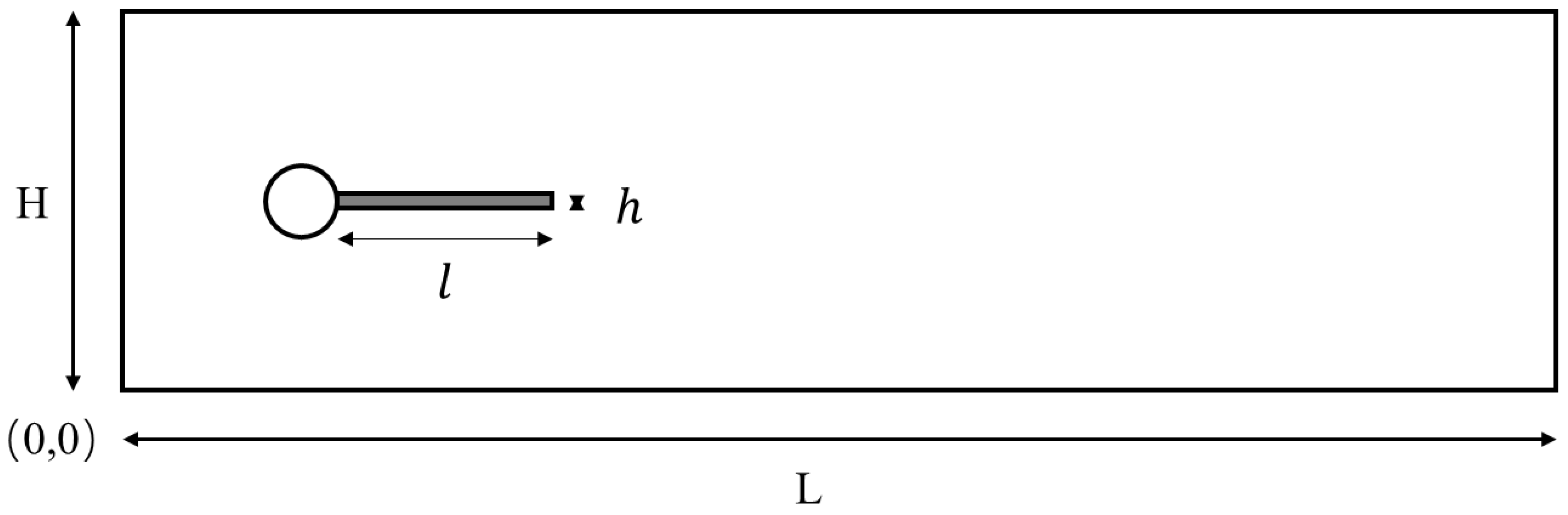
The benchmark case proposed by Turek and Hron, shown in Figure 2, is a flexible cantilever beam connected behind a cylinder. The dimensions of the computing domain are long $L=2.5$ and high $H=0.41$. The center of the circle around the flow cylinder is located at the point (0.2, 0.2) and the radius is r = 0.05. The length of the flexible cantilever is $l=0.35$ and the height is h = 0.02.

Figure 2. Model setup for flow-induced vibration of a flexible beam attached to a rigid cylinder.

The inlet boundary condition is a parabolic velocity distribution, and the velocity distribution function is shown in Equation (29), where $\overline{U}$ denotes the average incoming flow velocity, and the maximum incoming flow velocity at the parabolic inlet is $1.5\overline{U}$. We set the reference pressure at the outflow to have a zero mean value, and the other boundary conditions are set as non-slip wall boundary conditions. The inlet speed distribution is set to grow smoothly to the desired speed over time, as shown in Equation (30).

$$v^f\left(0,y\right)=1.5\overline{U}{\displaystyle \frac{y\left(H-y\right)}{{\left(H/2\right)}^2}},$$

(29)

$$v^f\left(t,0,y\right)=\left\{\begin{array}{c}{0.5·v}^f\left(0,y\right)·\left(1-cos\left(0.5\pi t\right)\right) t<2.0\\ v^f\left(0,y\right) t\ge 2.0\end{array}\right.,$$

(30)

Considering the numerical verification of fluid–structure interaction under two working conditions (1) ${\rho }_s/{\rho }_f=10,Re=\overline{U}d/\nu =100$ and (2) ${\rho }_s/{\rho }_f=1,Re=200$, the physical quantity parameters used are ${\rho }_f=1\times {10}^3\mathrm{k}\mathrm{g}/{\mathrm{m}}^3,\nu =1\times {10}^{-3}{\mathrm{m}}^2/\mathrm{s}, Ae={\displaystyle \frac{E}{\left({\rho }_f·{\overline{U}}^2\right)}}=1.4\times {10}^3,v_s=0.4, \mathrm{w}\mathrm{h}\mathrm{e}\mathrm{r}\mathrm{e}$ ${\rho }_s$ is material density, ${\rho }_f$ is fluid density, $d$ is the diameter of the cylinder, $Re$is the Reynolds number, $\nu$ is the kinematic viscosity coefficient, E is the elastic modulus, and $v_s$ is Poisson’s ratio. These two working conditions are referred to as FSI2 and FSI3 in the literature [39], and these terms will continue to be used in this paper.

3.2. Validation of the Fluid Solver

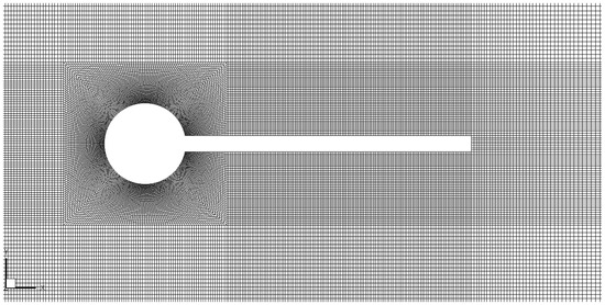
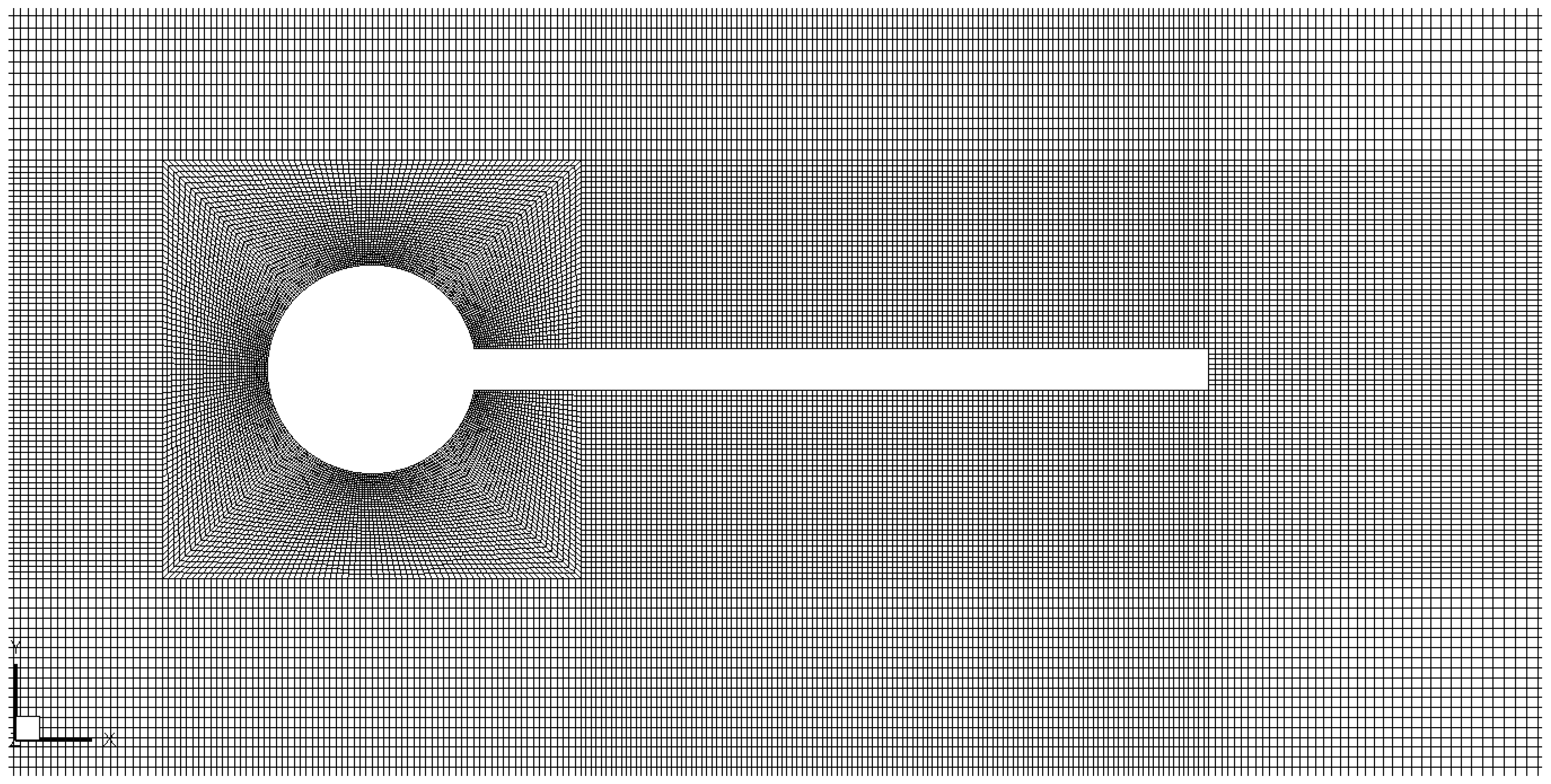
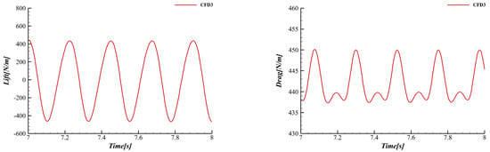
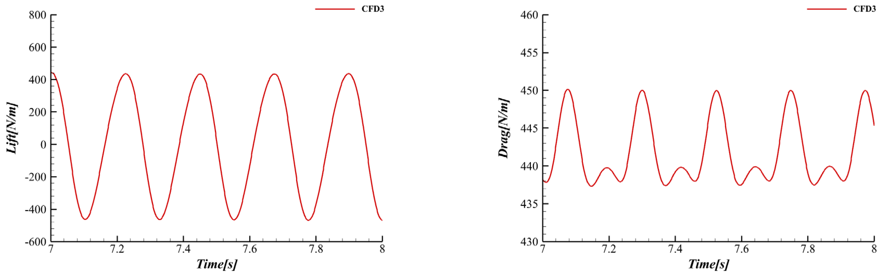
In this part, the flow fields in FSI2 and FSI3 are separately calculated and verified, which are referred to as CFD2 and CFD3 in the literature, and these terms will continue to be used. The incoming flow velocities $\overline{U}$ are $1\mathrm{m}/\mathrm{s}$ and $2\mathrm{m}/\mathrm{s}$ in CFD2 and CFD3 and the other solution settings of the flow fields are the same. The generation diagram of the fluid grid is shown in Figure 3, and the places close to the wall and the wake area are densified. Different densification levels result in meshes of different fineness. The time step is selected as 0.001 s. According to the results of Turek et al. [40], the authors think it is appropriate to choose this time step. It can take less time while ensuring the accuracy of the calculation. In order to verify the convergence of fluid meshes, three different fineness meshes named coarse, middle and refine are provided here, and the number of meshes corresponding to them is 25 k, 46 k and 120 k. Table 1 gives the calculation results in detail. From the table, we can see that the result of the middle mesh is close to that of the refine mesh and their values are all close to the reference value. For the sake of accuracy and time cost, we will use the middle grid in the following calculations. Figure 4 shows the calculated lift and drag curves for the CFD3 case with a mesh cell number of 46 k.

Figure 3. Fluid mesh diagram.

Table 1. Comparison of lift and drag value with the result given by Turek & Hron.

Case	CFD2		CFD3
	Drag	Lift	Drag	Lift	F
Coarse	140.2	10.76	450.69 ± 6.15	−10.93 ± 480.43	4.50
Middle	137.0	10.55	443.63 ± 6.16	−11.69 ± 455.61	4.46
Refine	136.9	10.54	442.38 ± 6.11	−11.87 ± 453.06	4.45
Turek & Hron	136.7	10.53	439.45 ± 5.62	−11.89 ± 437.81	4.40

Figure 4. Lift and drag force acting on the whole structure in the case of CFD3.

3.3. Validation of the Multibody Dynamics Solver

According to the literature [39], the structural test only calculates the structural deformation of the elastic beam under the action of gravity. The beam is loaded only with gravitational force $g=2\mathrm{m}/{\mathrm{s}}^2$, CSM2 is the structural statics solution, and CSM3 is the dynamic solution. MBDyn developed a finite volume multibody beam element to model elastic beams, and each beam element contains three nodes [41]. This beam element uses the C0 beam model and is discretized based on the concept of finite volume. The C0 beam is an important beam model that removes the simplifying assumption of zero shear deformation of Euler beams. The finite volume method is adopted for numerical implementation of the governing equations in the beam element. The finite volume beam element allows us to simulate the elastic deformation of bodies undergoing large displacements and rotations. Its main disadvantage is that both linear and linearized beam matrices lose symmetry. Therefore, the method is especially suitable for dynamic problems, where the symmetry of the matrix is not so important.

The beam is defined by a regular reference line $p$, and the position of any point $p\left(\xi \right)$ on the beam reference line is uniquely identified by the value of the abscissa $\xi$. The equilibrium equation of the beam is described in Equation (31), where $\vartheta$ denotes internal forces and moments, $\tau$ denotes external loads, and the prime denotes differentiation with respect to $\xi$.

$${\vartheta }^{\prime }-T^T\vartheta +\tau =0$$

(31)

The matrix $T$ is defined as follows:

$$\left[\begin{array}{cc}0& p^{\prime }\times \\ 0& 0\end{array}\right]$$

The finite volume approach can be interpreted as a weighted-residuals weak formulation of the equilibrium of a finite part of the beam. The equation is described in Equation (32), where $w$ is a weight function which takes a unit value in the domain [a, b]. For more technical details, please refer to Ghiringhelli et al. [41].

$${\int }_a^{b}w\left({\vartheta }^{\prime }-T^T\vartheta +\tau \right)d\xi =0$$

(32)

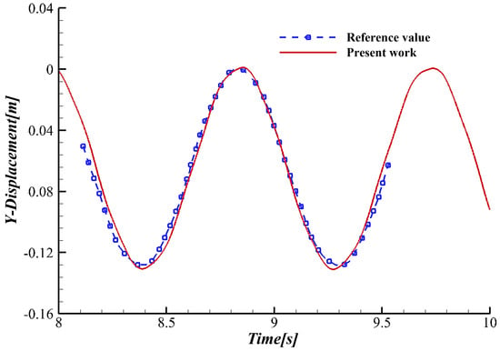
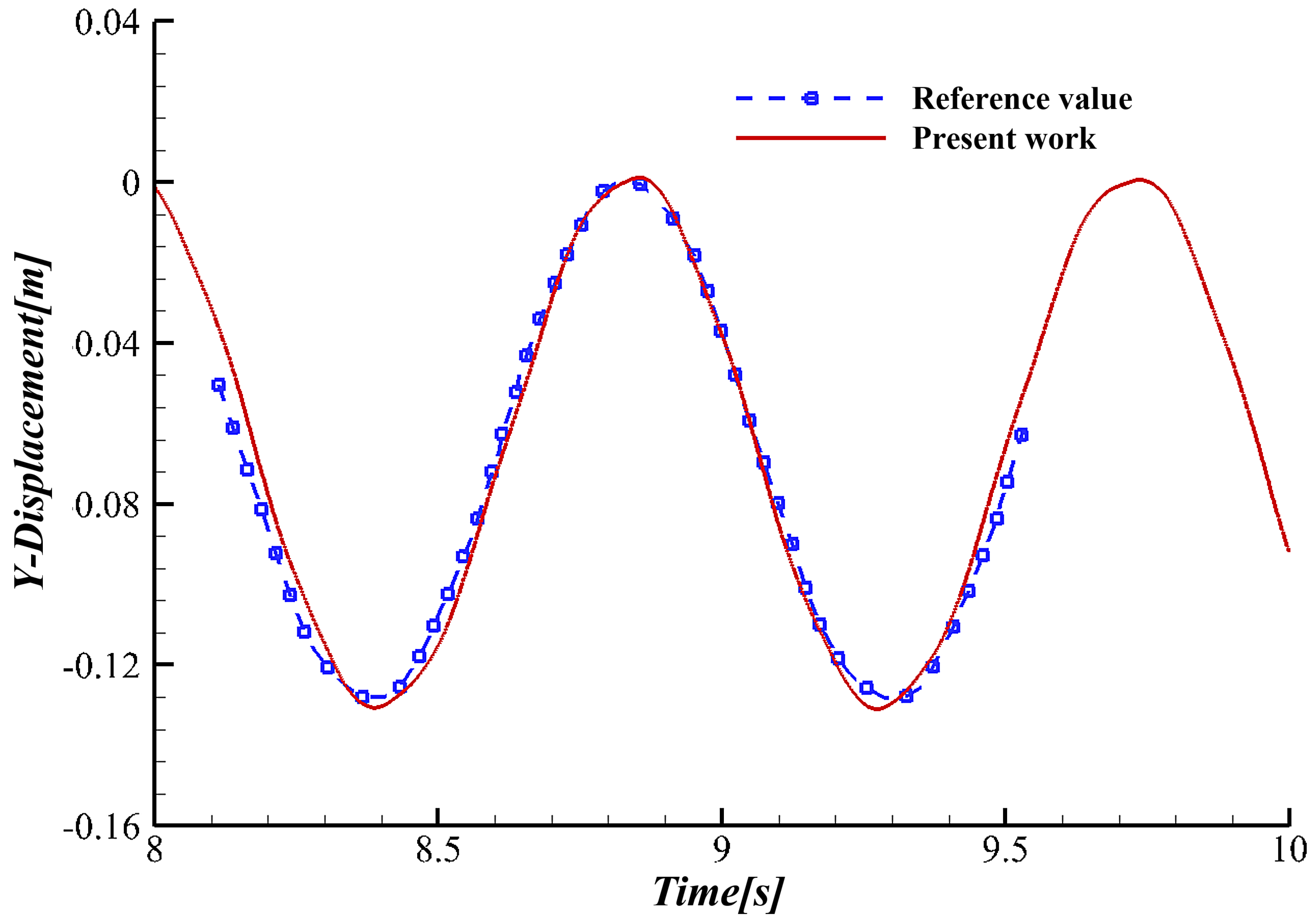
In Figure 5, the author shows the grid diagram of the beam, in which the blue and yellow points represent structural nodes, and every three structural nodes form a beam element. The beam section is rectangular, the section shape does not change along the beam length, and the structural parameters and material parameters are constant. The beam can be divided into several elements along the beam length direction. Figure 6 shows the displacement of the beam end point A in the y-direction in the case of CSM3 with a mesh cell number of 20 and compares it with the results of Turek and Hron. As the entire beam has a constant cross-section, all beam elements share identical cross-sectional properties. The Rayleigh structural damping coefficient for the C-beam elements in MBDyn was set to 2.5 × 10⁻⁵. The residual convergence tolerance was set to 1 × 10⁻⁶, and the maximum number of sub-iterations was set to 100. It can be seen that the calculated results are in good agreement with the literature results. In Table 2, the displacement and frequency of point A in the case of CSM2 and CSM3 are given in detail, where $u_x$ represents the displacement of point A in the x-direction, $u_y$ represents the displacement of point A in the y-direction, and F is the frequency. The result of the mesh is close to the reference value. Thus, we will use this grid in the following calculations.

Figure 5. Schematic diagram of cantilever beam.

Figure 6. Comparison displacement of point A in the y-direction with Turek & Hron in the case of CSM3.

Table 2. Comparison of result with Turek & Hron in case of CSM2 and CSM3.

Case	CSM2		CSM3
	$u_x$	$u_y$	$u_x$	$u_y$	F
Present work	−0.47	−17.08	−14.25 ± 14.25	−65.05 ± 65.19	1.10
Turek and Hron [39]	−0.47	−16.97	−14.31 ± 14.31	−63.61 ± 65.16	1.099

3.4. Validation of the Fluid–Structure Interaction Framework

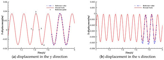
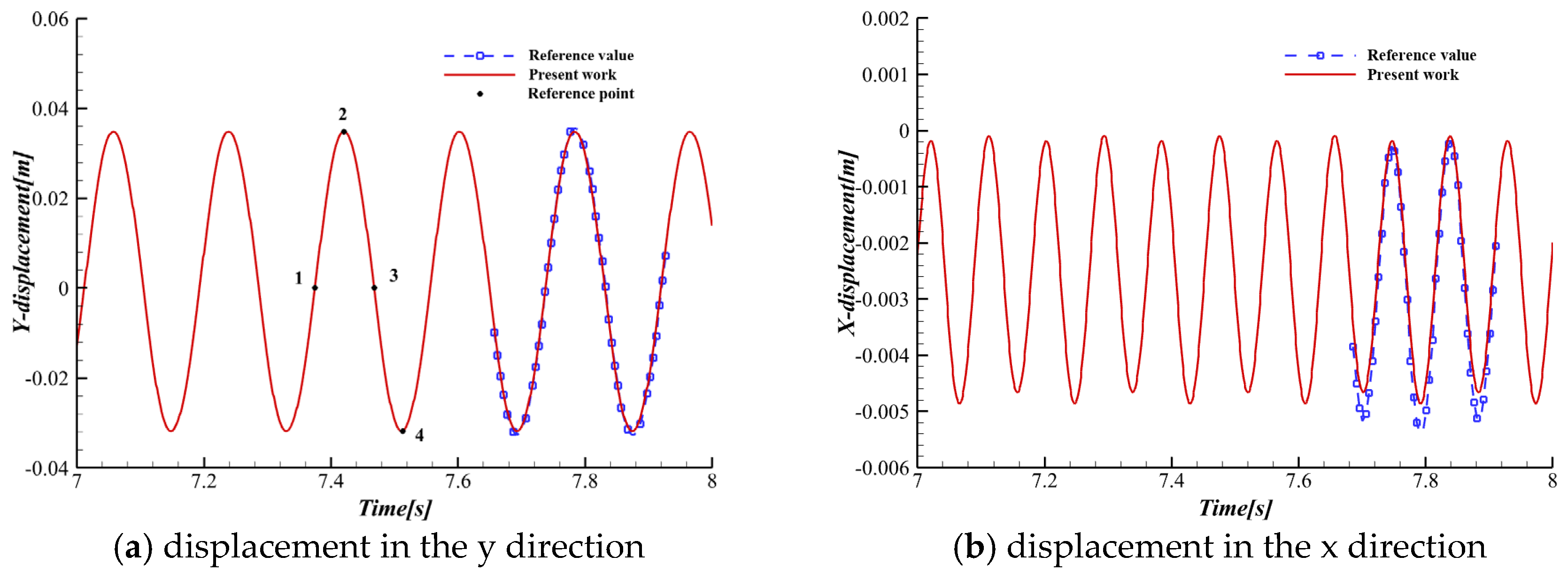
After validation of the fluid and structure parts, the fluid–structure interaction solver was further tested. Figure 7 shows the comparison of the present work with Turek & Hron in the x and y-direction of point A (marked in Figure 5) in the case of FSI3. It can be seen from Figure 7a that in the y-direction displacement, the calculated results in this paper and the results in the reference have maintained good consistency in amplitude and period. From Figure 7b, we can see that the displacement in the x-direction is slightly larger in magnitude than the results in the reference. The reason for the error is that this paper uses a different numerical method from the reference, and the x-direction displacement value itself is small. Figure 8 gives the pressure contours and streamlines at four time instances labeled in Figure 7a. From the figure, we can see that the periodic variation in beam tip displacement and pressure contours shows good agreement between the present and published results [39]. In Table 3, the results for CSM2 and CSM3 are given in detail, where $A_m$ represents the maximum displacement amplitude in the $y$-direction of the beam tip, $d$ is the cylindrical radius, $St=f\overline{U}/d$, $f$ is the vibration frequency, $Cd=F_x/\left(0.5{\rho }_f\overline{U}{d}^2\right)$, and $F_x$ is the average drag force acting on the whole structure. As can be seen from the table, the calculation results obtained in this paper are consistent with the references. This means that the proposed framework in this paper can simulate the FSI phenomena. In next section, we will calculate flexible multibody models in detail.

Figure 7. Comparison displacement of point A with Turek & Hron in the case of FSI3.

Figure 8. Pressure contours and streamlines corresponding to the four time points marked in Figure 7a.

Table 3. FSI2 and FSI3 validation.

Case	Sources	${\mathit{A}}_{\mathit{m}}/\mathit{d}$	St	Cd
${\rho }_s/{\rho }_f=10,Re=100$	Present result	0.80	0.19	4.18
	Turek and Hron [39]	0.83	0.19	4.16
	Tian et al. [42]	0.78	0.19	4.11
${\rho }_s/{\rho }_f=1,Re=200$	Present result	0.35	0.28	2.30
	Turek and Hron [39]	0.36	0.26	2.30
	Tian et al. [42]	0.32	0.29	2.16

4. The Unsteady Flow of a Cylinder with Flexible Multibody Beams

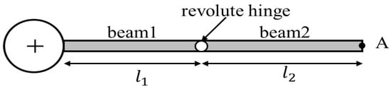
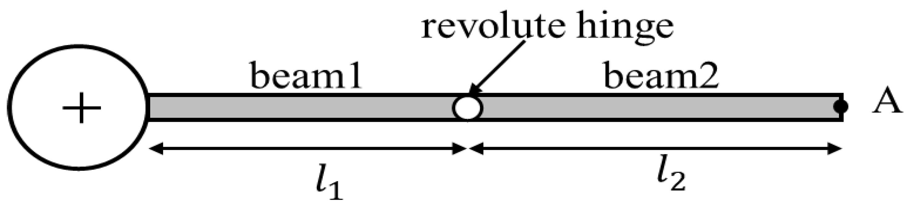
On the basis of verification of FSI2 and FSI3, we add a hinge to the single flexible beam, creating a multibody system formed by two beams connected by a revolute hinge, as shown in Figure 9. The length of beam1 is $l_1$, the length of beam2 is $l_2$, and the sum of the lengths of the two beam is$l$. $l$ is a fixed value equal to the length of the single flexible beam in the validation. Point A is the tip of beam2. We define $\phi =l_1/l$ by taking different values of $\phi$ to represent the different positions of the hinge. Firstly, we take $\phi$ as 0.5. The influence of the hinge is analyzed by comparing it with the original single flexible beam case. Secondly, we take $\phi$ as 0, 0.125, 0.25, 0.375, 0.625, 0.75, 0.875, and 1, and analyze the influence when the hinge is in different positions. When the value of $\phi$ is set to 1, it represents the FSI3 example model calculated in Section 3. In the charts used in this section, we will use “original” to represent this situation. When the value of $\phi$ is set to 0, the structural model represented at this time comprises the cylinder and beam connected together through hinges instead of the previous fixed connection. In this section, the inlet flow state and boundary conditions are adopted to be the same as the parameters in FSI3, so as to facilitate our subsequent comparison, and will not be repeated here.

Figure 9. Structure diagram.

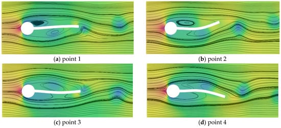
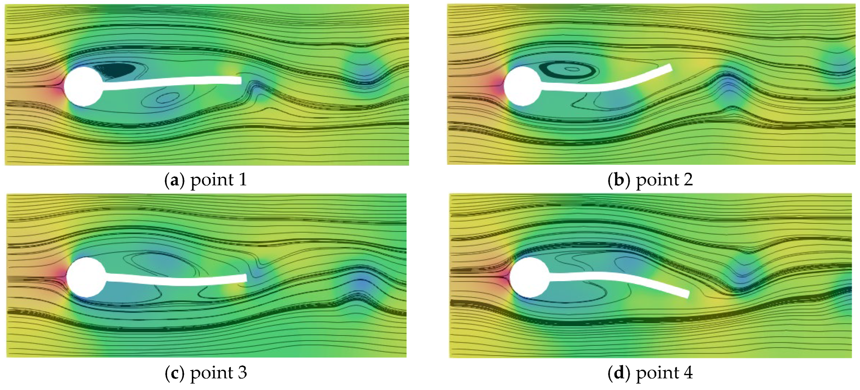
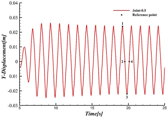
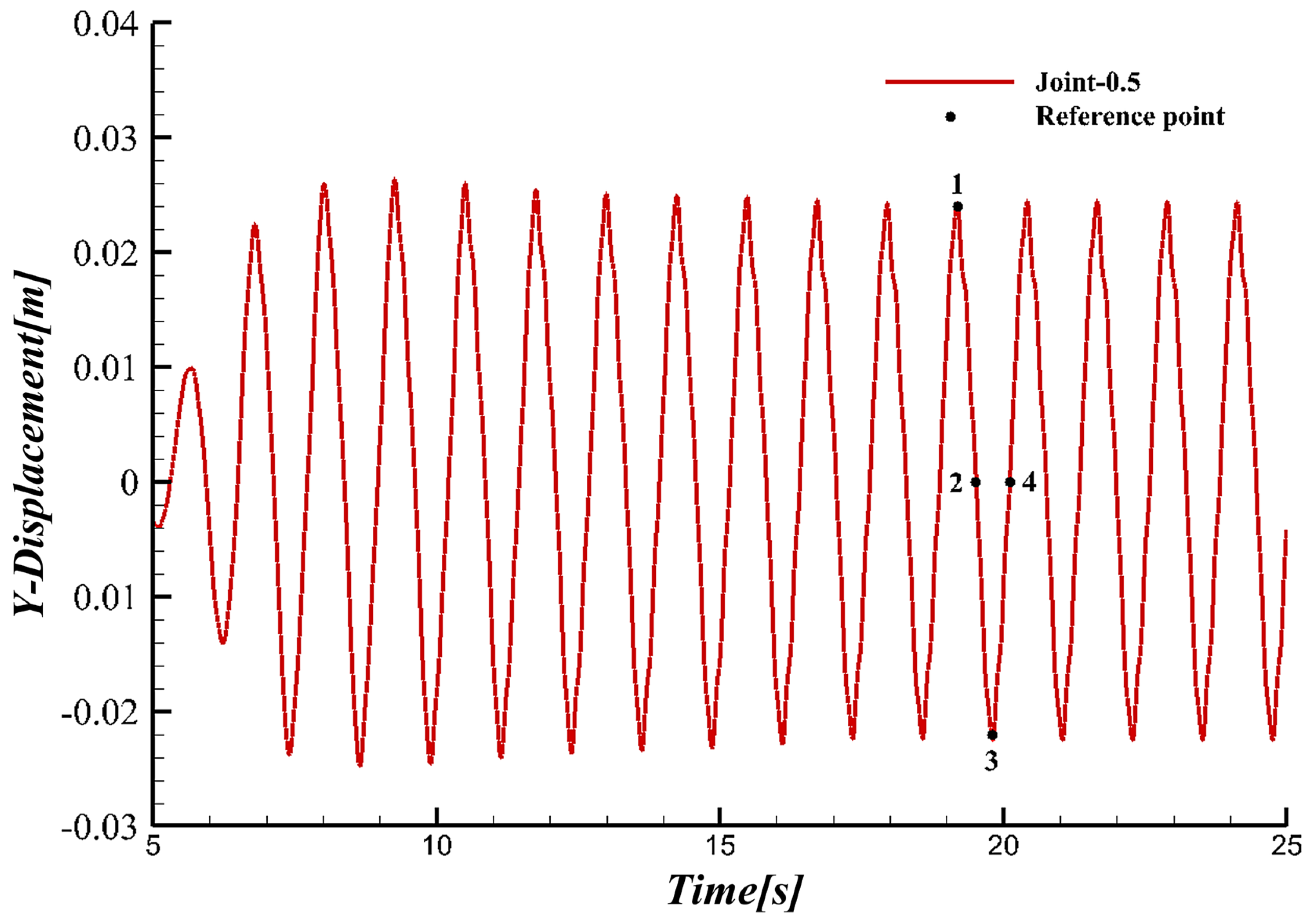
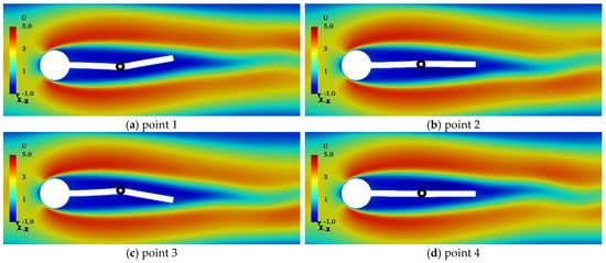
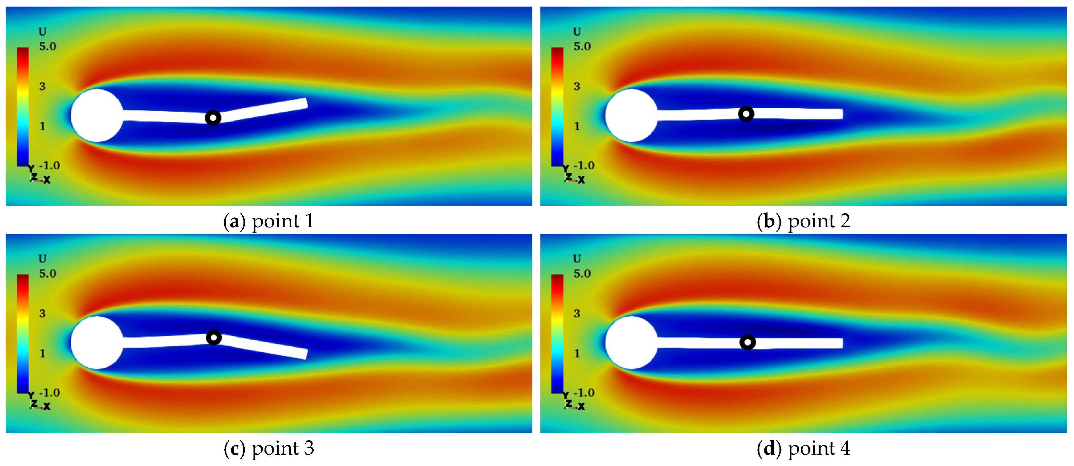
When the value of $\phi$ is 0.5, flexible beam1 and beam2 are the same length. Figure 10 shows the y-direction displacement image of point A within 5 to 25 s. After 15 s, the numerical simulation results are close to stability, and the displacement curve shows periodicity. Compared with the original situation, the period of the displacement curve is longer and the amplitude is smaller. This means that the swing of the structure in the flow field is slow and of small magnitude. On the displacement curve, four reference points are marked, and they form a swing cycle; the velocity contours corresponding to the four reference points are given in Figure 11. From the figure, we can see that the deformation of beam1 in the flow field is small, while beam2 has a large deflection in the flow field. This is precisely because the presence of the hinge releases the rotational constraint, so a small force change in the flow field can quickly cause the deflection of beam2.

Figure 10. Displacement in y-direction at point A.

Figure 11. Velocity contours corresponding to the four time points marked in Figure 10.

Comparison of Displacement at Point A with Different φ Values

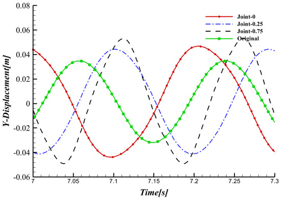
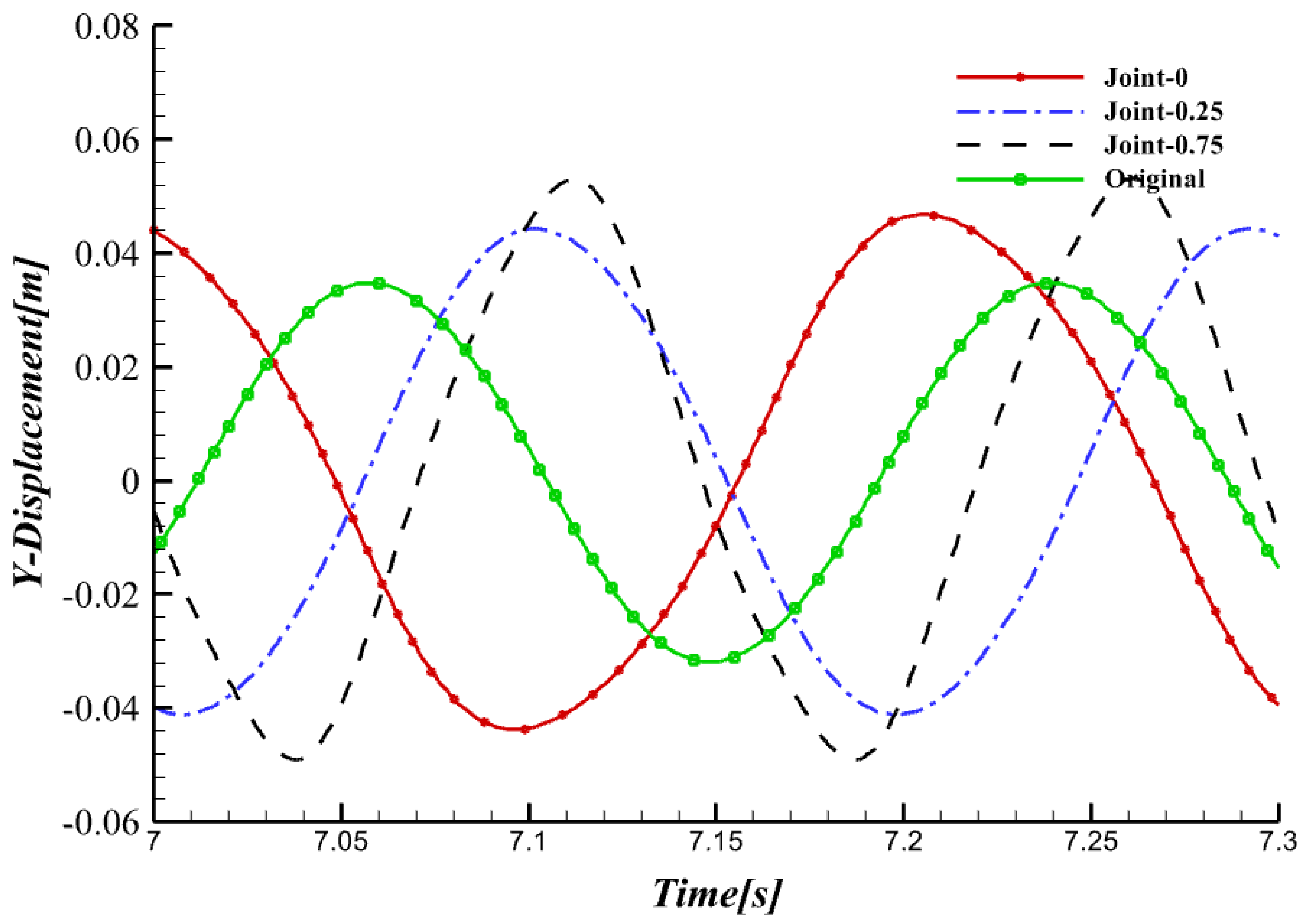
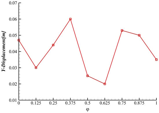
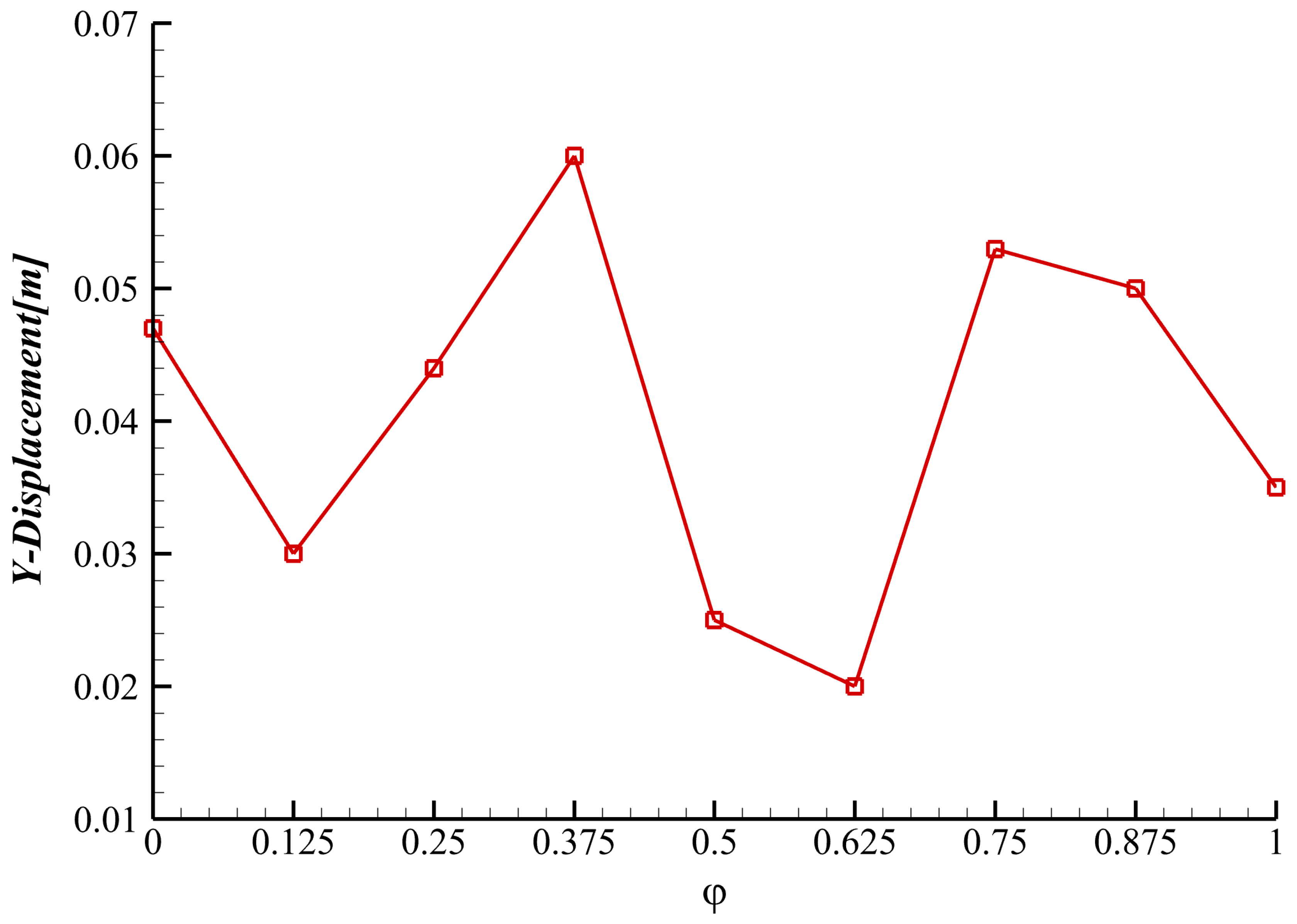
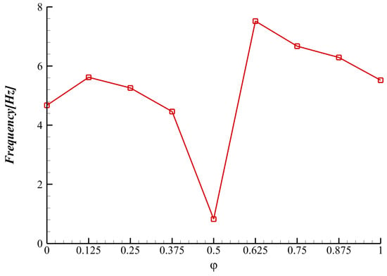
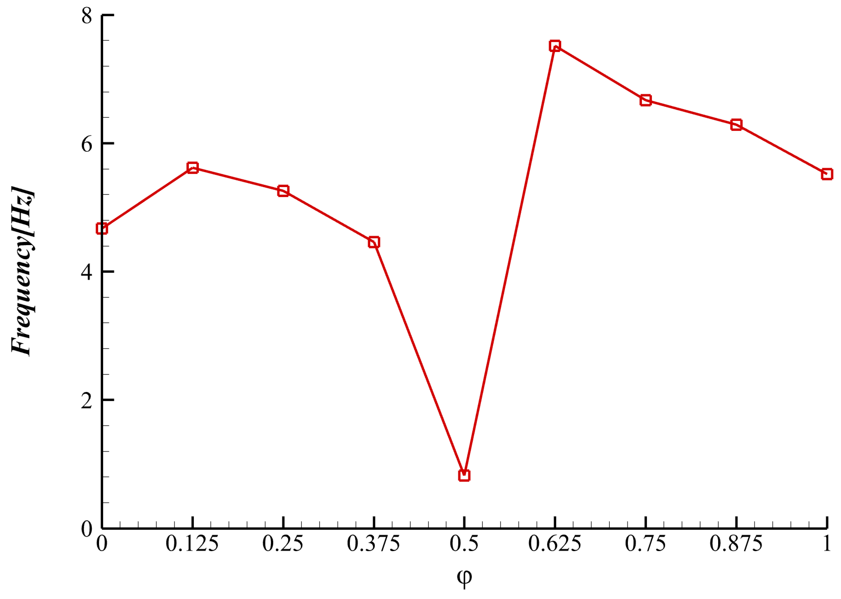
Taking $\phi$ as 0, 0.125, 0.25, 0.375, 0.5, 0.625, 0.75, 0.875, and 1, periodic phenomena appear in the displacement at point A in the y-direction, which means that the structure oscillates periodically in the flow field. In order to keep the figure clearly visible, the displacement curves corresponding to all $\phi$ values will not be listed one by one here; only the displacement when the $\phi$ value is 0, 0.25, 0.75, and 1 in the time range of 7 to 7.3 s is displayed in the same graph, as shown in Figure 12. It can be seen from the figure that, relative to the original case, the displacement amplitude increases in all three cases, among which the largest increase is when $\phi$ is taken as 0.75. For a better comparison, we show the displacement amplitude corresponding to each $\phi$ value in Figure 13. From the figure, we can see that when the $\phi$ value is taken as 0.125 and 0.625, the displacement amplitude is smaller than the original case, and the displacement amplitude in the other cases is larger than that of the original case. When the value of $\phi$ is less than 0.5, the displacement amplitude shows a trend of first decreasing and then increasing, while when the value of $\phi$ is greater than 0.5, it shows a trend of first increasing and then decreasing. Interestingly, we observe that the maximum and minimum values occur at $\phi$ values of 0.375 and 0.625. Their $\phi$ values are all close to 0.5, but the corresponding displacement amplitudes have changed so much that the corresponding amplitude when $\phi$ takes 0.375 is almost three times that of 0.625. This shows that the region where the $\phi$ value corresponding to the hinge position is close to 0.5 is a sensitive region, and the hinge position in this region has a greater impact on fluid–structure interaction characteristics. Next, we will analyze these two cases separately. In Figure 14, we have given the vibration frequency of the structure; it can be observed that the structure has the longest period of oscillation when $\phi$ is taken as 0.5 and this phenomenon can also be seen in the previous section. When $\phi$ is taken as 0.625, the structure has the fastest frequency of oscillation.

Figure 12. Displacement of point A in y-direction when $\phi$ is taken as 0, 0.25, and 0.75.

Figure 13. Comparison of displacement amplitudes of point A in y-direction under different $\phi$ values.

Figure 14. The frequency of periodic movement of the structure under different $\phi$ values.

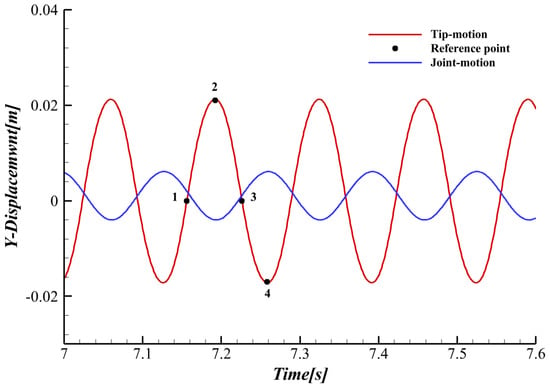
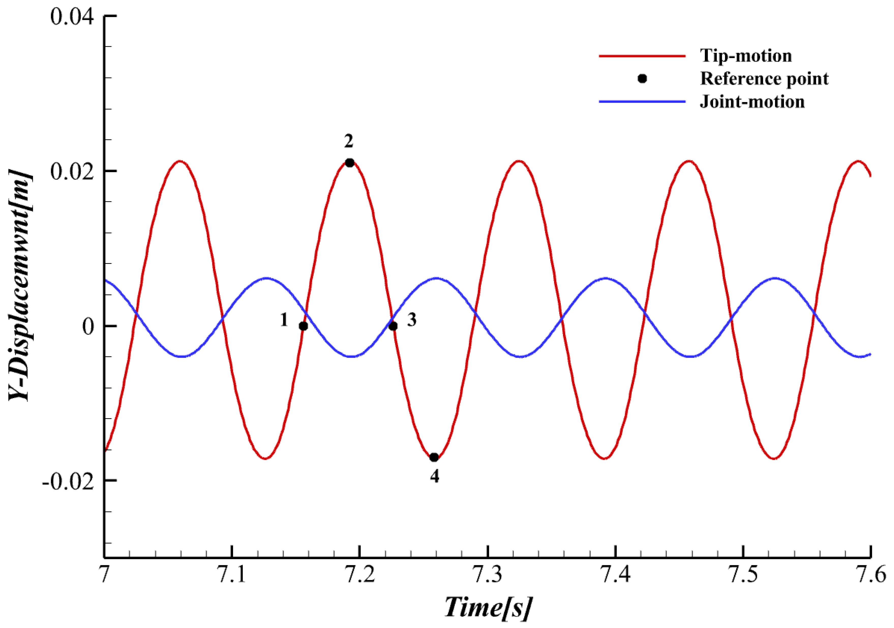
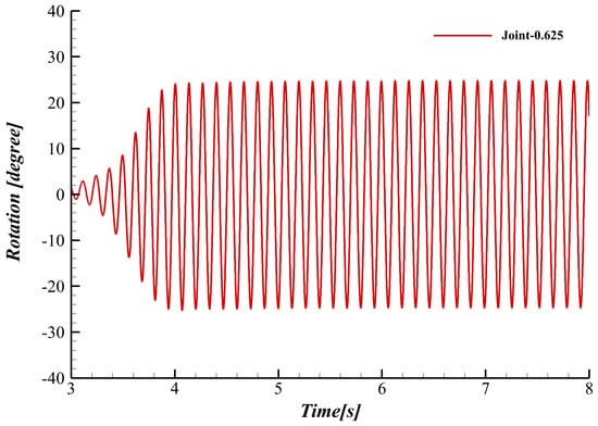
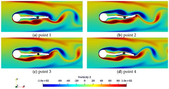
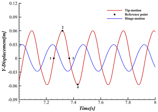
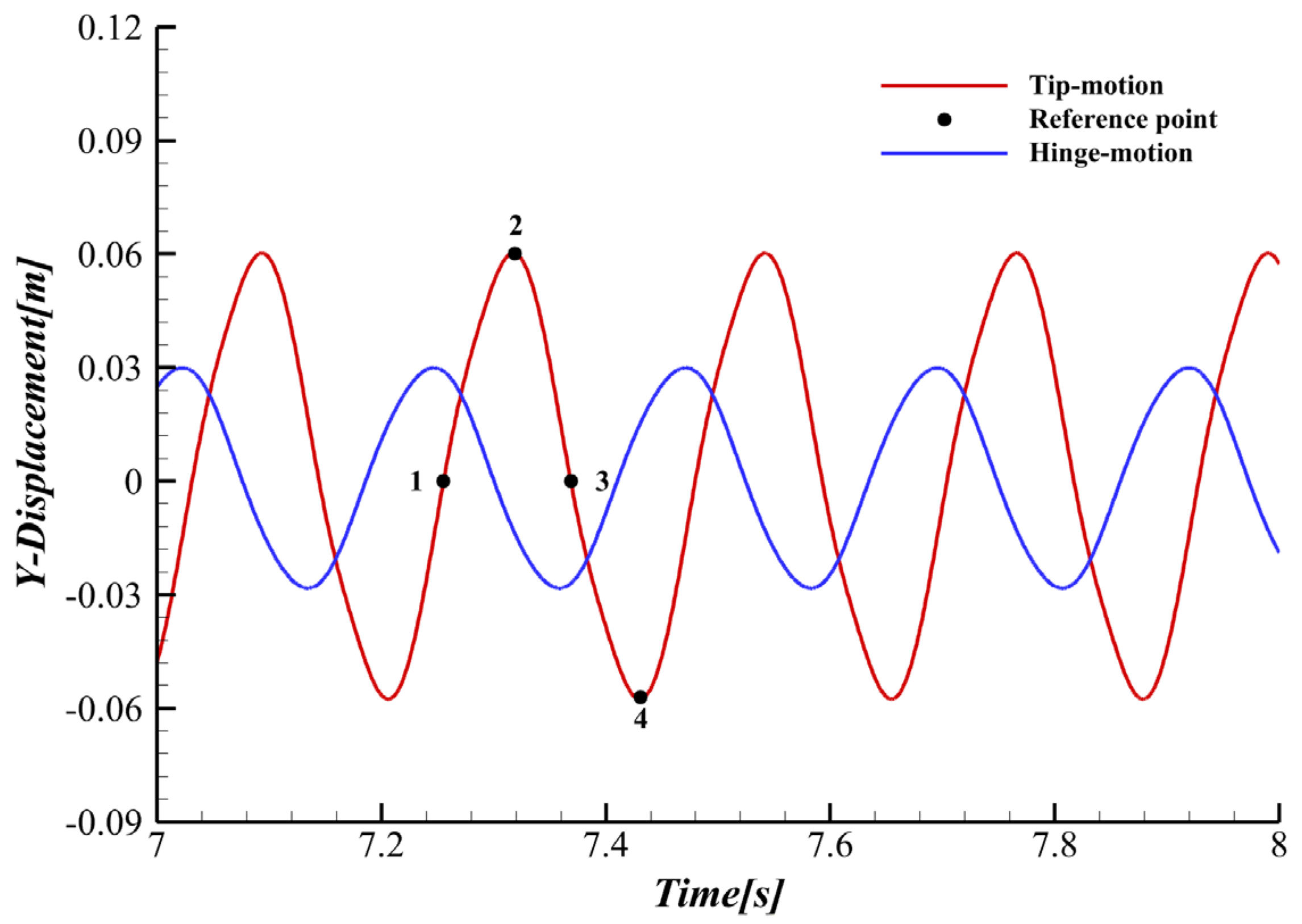
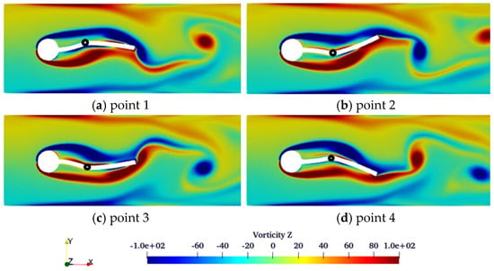
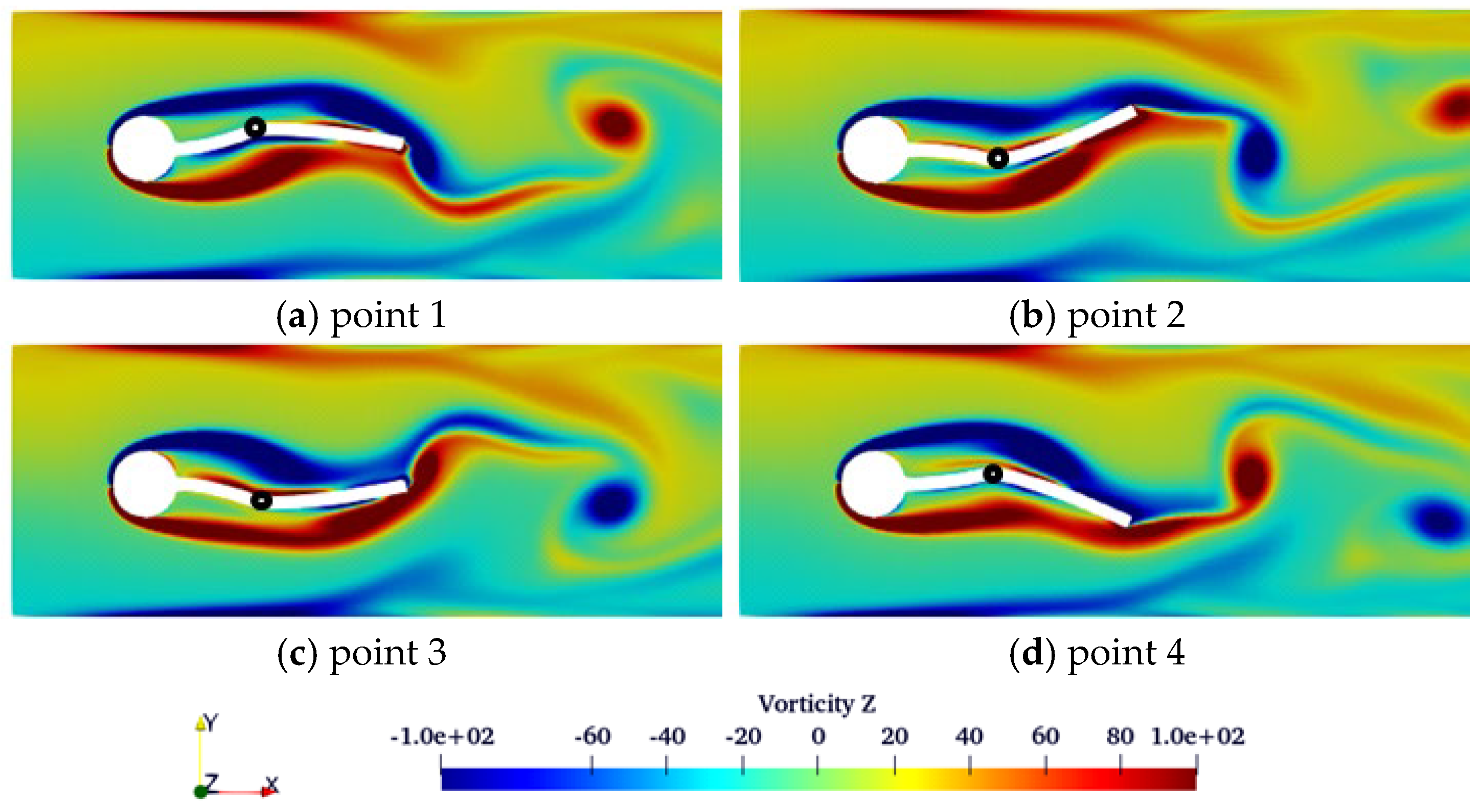
Figure 15 shows the y-direction displacement curve of tip point A and the joint when the value of $\phi$ is taken as 0.625 within 7 to 7.6 s. It can be seen from the figure that the amplitude of the displacement of the hinge is small relative to that of tip point A. This means that the amplitude of the oscillation of beam1 is smaller than that of beam2. Figure 16 shows the curve of the hinge rotation angle over time, and it can be seen that the maximum rotation angle of the hinge is close to 25 degrees. During one displacement cycle, shown in Figure 15, four reference points are marked. In Figure 17, the z-direction vorticity cloud map at the time corresponding to the four marked points is given. The small black circles in the diagram represent where the hinges are located. Observing the four pictures included in Figure 17, we can find that two vortex structures are formed on the upper and lower surfaces of the beam, and these vortices shed alternately to form periodic forces acting on the two beams, causing the structure to periodically oscillate in the flow field. In Figure 17a, on beam2, the counterclockwise vortex on the lower surface has been shed, and the clockwise vortex on the upper surface is shedding. The clockwise vortex on the upper surface creates an area of low pressure, which causes an upward force on beam2, pushing beam2 to deflect upwards. On beam1, compared with the clockwise vortex on the upper surface, the counterclockwise vortex on the lower surface is stronger and fuller in shape, and the action area is further back. The action of the upper and lower surface vortices will deform the beam, gradually forming the shape shown in Figure 17b. In Figure 17b, on beam2, the clockwise vortex on the upper surface is shedding, and the counterclockwise vortex on the lower surface is developing along beam2. The low-pressure area formed by the counterclockwise vortex on the lower surface will push beam2 to deflect downwards, thereby gradually returning to the horizontal position. On beam1, the clockwise vortex on the upper surface is stronger, fuller in shape, and more rearward than the counterclockwise vortex on the lower surface. Beam1 will return to the horizontal position, resulting in the situation shown in Figure 17c. In the same way, it can be analyzed that under the action of the vortex in Figure 17c, the structure will deform into that shown in Figure 17d, and finally return to that shown in Figure 17a, forming a complete cycle. In summary, in one swing period, when beam1 swings upward, beam2 swings downward. While beam1 swings downward, beam2 swings upward. The two beams are balanced in the flow field by swinging in opposite directions. The vortex generated after the cylinder acts on the two beams then falls off and develops downstream.

Figure 15. Displacement of tip point A (red line) and hinge (blue line) in y-direction when $\phi$ is taken as 0.625.

Figure 16. Curve of rotation angle of hinge with time when $\phi$ is taken as 0.625.

Figure 17. Vortex contours in the z-direction corresponding to the four time points marked in Figure 15.

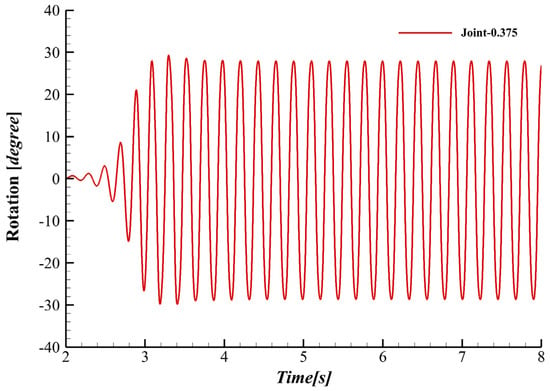
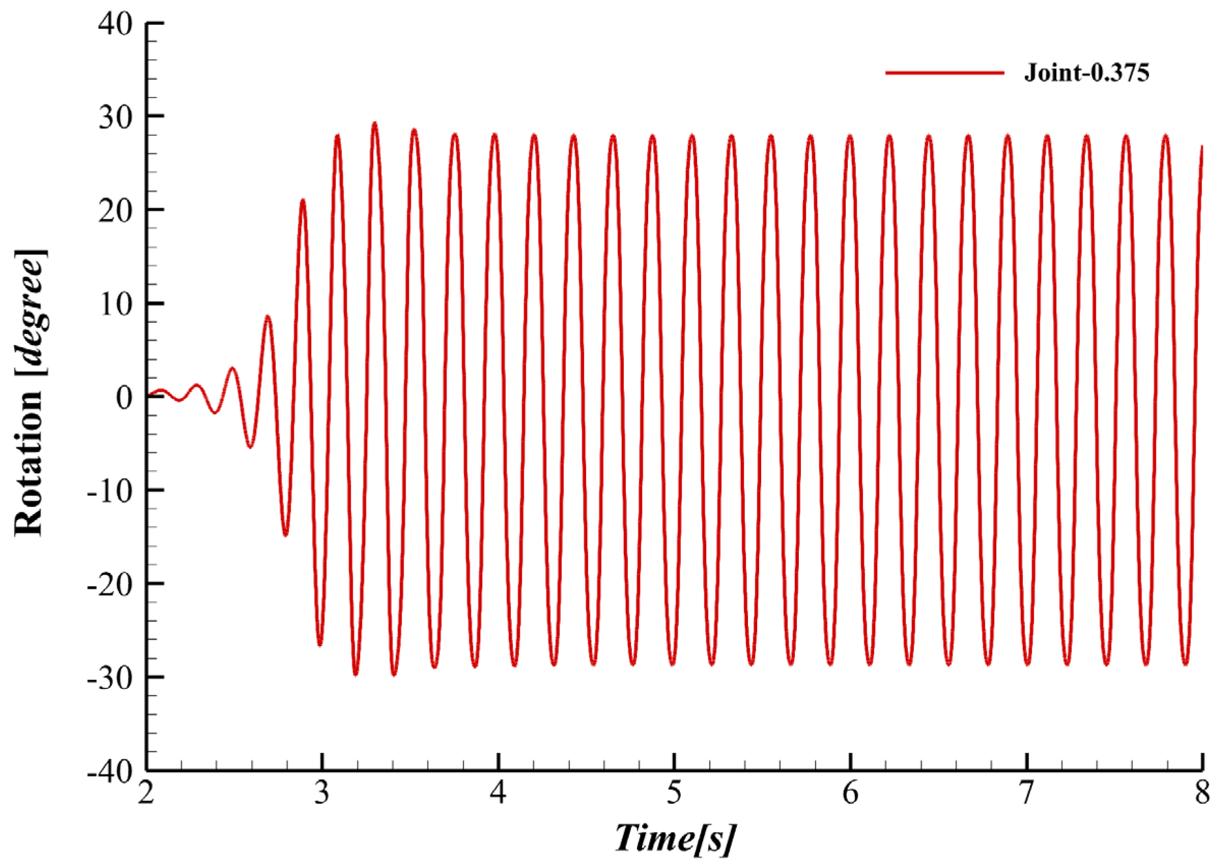
Figure 18 shows the y-direction displacement curve of tip point A and the hinge when the value of $\phi$ is taken as 0.375 within 7 to 7.6 s. Figure 19 shows the curve of the hinge rotation angle over time, and it can be seen that the maximum rotation angle of the hinge is close to 30 degrees. During one displacement cycle, shown in Figure 18, four reference points are marked. In Figure 20, the z-direction vorticity cloud map at the time corresponding to the four marked points is given. The small black circles in the diagram represent where the hinges are located. In Figure 20a, the clockwise vortex on the upper surface of the beam is shedding, forming a low-pressure area at the tip of beam2, and the counterclockwise vortex on the lower surface is developing, forming a low-pressure area at the front end of beam2. Under the action of the upper and lower surface vortices, beam1 will bend downward, and beam2 will deflect upward, forming the situation shown in Figure 20b. In Figure 20b, the clockwise vortex on the upper surface has been shed, and the counterclockwise vortex on the lower surface is developing forward along beam2, causing beam2 to be deflected downward, forming the situation shown in Figure 20c. In the same way, it can be analyzed that under the action of the vortex in Figure 20c, the structure will deform into that shown in Figure 20d, and finally return to that shown in Figure 20a, forming a complete cycle.

Figure 18. Displacement of tip point A and hinge in y-direction when $\phi$ is taken as 0.375.

Figure 19. Curve of rotation angle of hinge with time when $\phi$ is taken as 0.375.

Figure 20. Vortex contours in the z-direction corresponding to the four time points marked in Figure 18.

We now compare the occurrence and evolution forms of vortices in the two cases. When $\phi$ is taken as 0.625, beam1 is longer, and the vortex formed after the cylinder will first act on beam1, causing the structure to deform, and then develop downward along beam2 until it falls off and develops downstream. It is this form that allows the structure to form a balance in the flow field with a small oscillation amplitude. When $\phi$ is taken as 0.375, the vortex formed behind the cylinder acts directly on beam2. Due to the longer length of beam2, the action of the vortex will cause the beam to swing rapidly in the flow field, resulting in a larger swing amplitude.

The beam material has an elastic modulus of $E=5.6\times {10}^6 \mathrm{p}\mathrm{a}$, a Poisson’s ratio of 0.4, and a density of ${\rho }_s=1\times {10}^3\mathrm{k}\mathrm{g}/{\mathrm{m}}^3$. The beam has a rectangular cross-section with a width of 0.01 m and a height of 0.02 m. For $\phi =0.375$ and $\phi =0.625$, the cantilever beam lengths are 0.13 m and 0.22 m, respectively. The natural frequencies are calculated using Euler–Bernoulli beam theory [43,44]. The first-order natural frequency is calculated as follows:

$$f_1={\displaystyle \frac{{1.8751}^2}{{2\pi L}^2}}\sqrt{{\displaystyle \frac{EI}{\rho A}}},$$

(33)

where $L$ is beam length, $A$ is the cross-sectional area, and $I$ is the second moment of area. The corresponding first-order natural frequencies are 13.77 Hz and 5.02 Hz, respectively

For the flow past the circular cylinder at $Re=200$, $\overline{U}=2 \mathrm{m}/\mathrm{s}$. The diameter of the cylinder is $D=0.1 \mathrm{m}$. The vortex shedding frequency is estimated as 3.94 Hz based on the method of Williamson and Brown [45]. The calculation formula is as follows:

$$\mathrm{S}\mathrm{t}=0.2731-1.1129/\sqrt{\mathrm{R}\mathrm{e}}+0.4821/\mathrm{R}\mathrm{e},$$

(34)

$$\mathrm{f}=\mathrm{S}\mathrm{t}\times \overline{\mathrm{U}}/\mathrm{D},$$

(35)

Thus, for $\phi =0.625$, the first natural frequency of the beam is closer to the vortex shedding frequency than that for $\phi =0.375$. Frequency proximity alone would therefore suggest a stronger resonance-related response at $\phi =0.625$. However, the computed vibration amplitudes show the opposite trend, with a larger amplitude at $\phi =0.375$.

This comparison indicates that the amplitude discrepancy cannot be explained solely by resonance or detuning between the structural natural frequency and the vortex shedding frequency. Instead, it is primarily associated with the location and interaction of the shed vortices relative to the flexible beam, as evidenced by the vortex contours.

5. Numerical Simulation of Fluid–Structure Interaction of a Continuously Morphing Swept Wing

5.1. Model Description

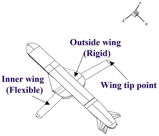
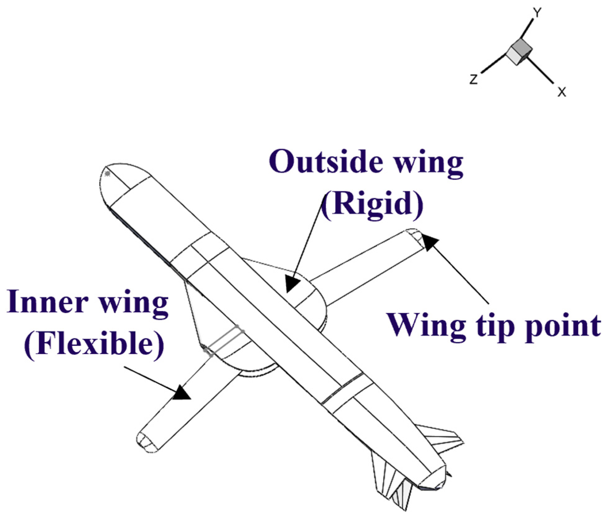
Furthermore, the multibody fluid–structure interaction numerical simulation method developed in this study is applied to the continuous morphing process of a variable-sweep wing. The designed variable-sweep wing model is shown in Figure 21. The model consists of a fuselage, an outer wing panel, and an inner wing panel. Following a rotational variable-sweep design concept, the outer wing section is nested within the inner wing section, and the inner wing section rotates to achieve sweep angle variation. The fuselage and inner wing section are designed as rigid bodies, while the outer wing section is modeled as a flexible structure.

Figure 21. Structural model of variable-sweep wing.

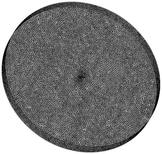
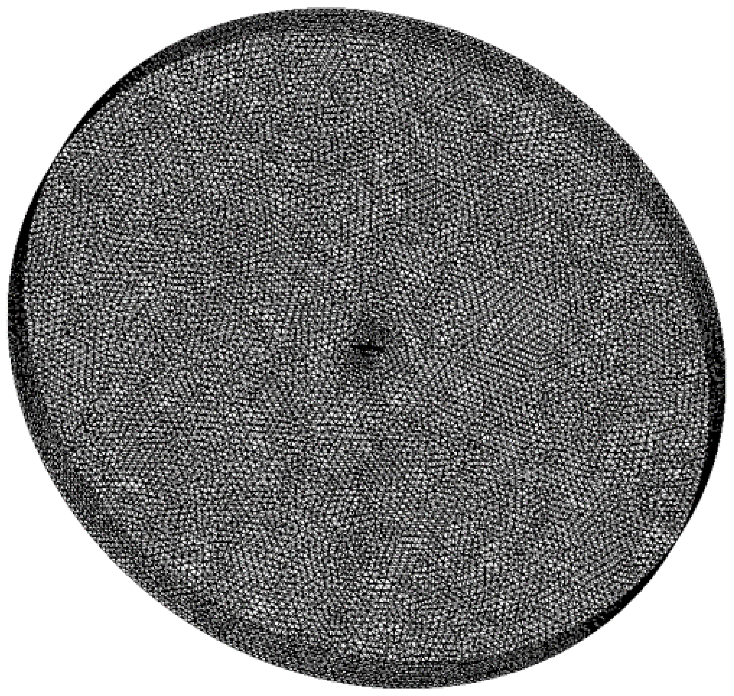
In Figure 22, the global computational mesh used in the simulations is shown. The computational mesh is three-dimensional and is constructed within a cylindrical computational domain with a radius of 15 L and a width of 5 L, where L denotes aircraft length. An unstructured tetrahedral mesh was employed, with local refinement in the near-wall regions to resolve the flow features around the aircraft surface. To assess grid independence, three meshes with different resolutions were tested: a coarse mesh (1.47 × 10⁶ cells), a medium mesh (3.15 × 10⁶ cells), and a fine mesh (5.88 × 10⁶ cells). The results obtained from these three meshes are summarized in Table 4. As shown in the table, the aerodynamic predictions from all three meshes are very close. Considering both accuracy and computational cost, the medium-resolution mesh is adopted for the subsequent simulations. A pressure-far-field boundary condition was imposed, with a freestream Mach number of 0.5 and an angle of attack of 0°. All aircraft surfaces were treated as no-slip wall boundaries, and turbulence was modeled using the $\mathrm{k}$-$\mathsf{\omega } \mathrm{s}\mathrm{s}\mathrm{t}$ model.

Figure 22. Global flow field mesh distribution.

Table 4. Grid independence verification.

Case	Drag(N)	Lift(N)	Error
Coarse	94.80	1374.16	1.8%
Middle	92.43	1388.91	0.8%
Refine	92.01	1400.35	-

5.2. Computational Results

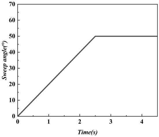
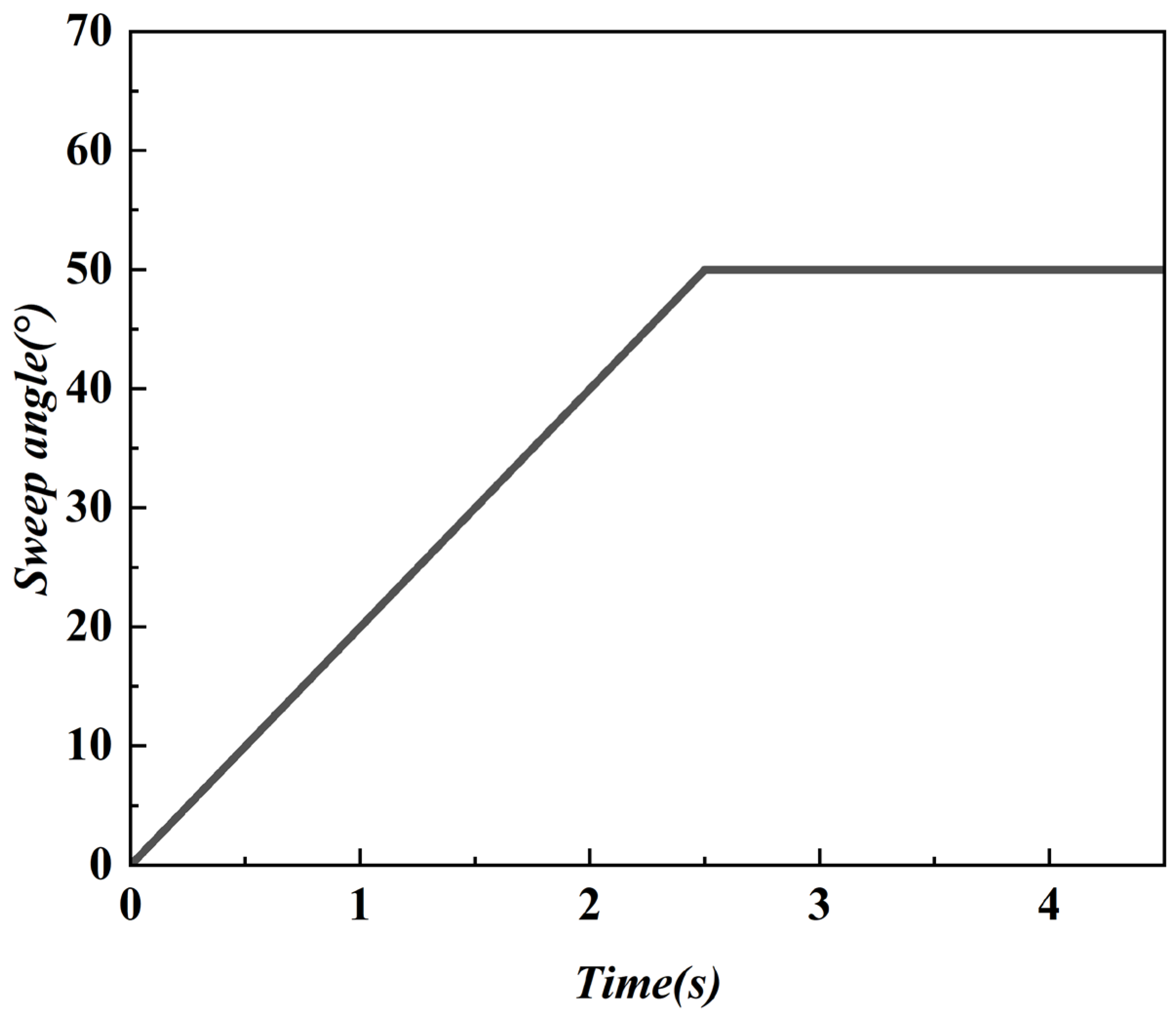
The inner wing panel is made of a linear elastic material with a Young’s modulus of 68 GPa and a Poisson’s ratio of 0.3. During the variable-sweep process, the inner wing panel rotates to achieve sweep variation. Over a period of 2.5 s, the sweep angle increases uniformly from 0° to 50°. Figure 23 shows the time history of the sweep angle during the active variable-sweep process.

Figure 23. Time history of wing sweep angle.

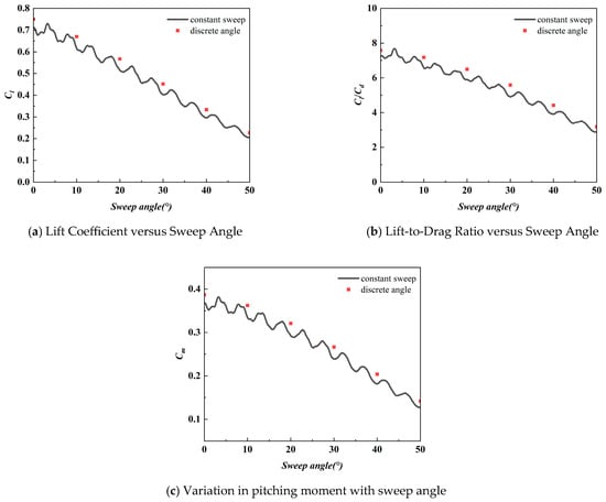
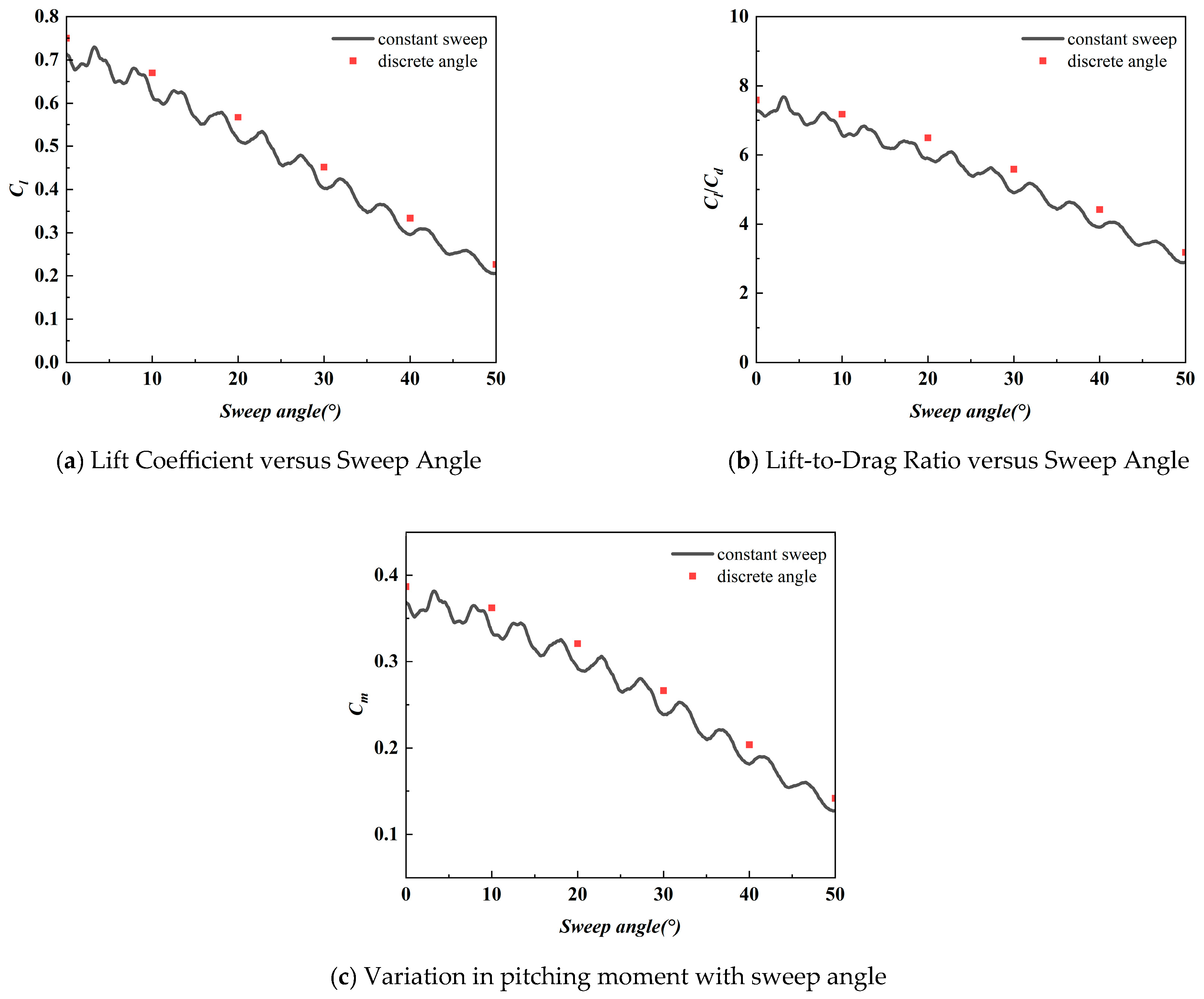
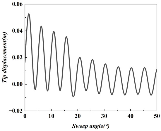
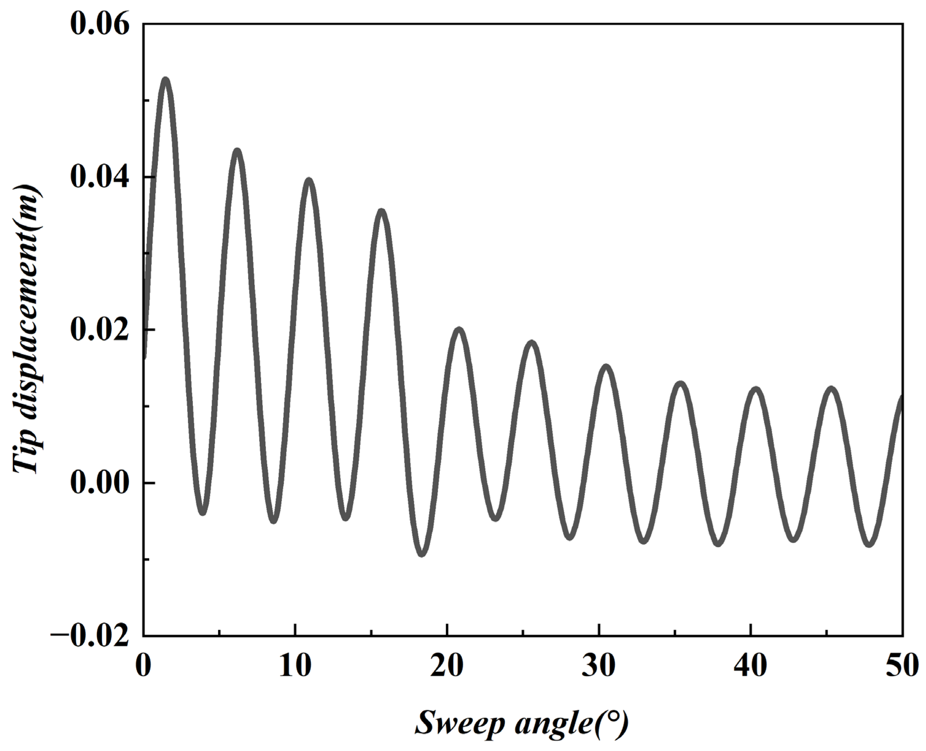
Figure 24 shows the variations in lift coefficient, lift-to-drag ratio, and pitching moment coefficient for an inflow Mach number of 0.5 and an angle of attack of 0°. The black curve represents the aerodynamic forces during the continuous deformation process, whereas the red markers denote the aerodynamic forces obtained at fixed sweep angles. As shown, the aerodynamic forces at fixed sweep angles are slightly higher, indicating that, in the presence of structural flexibility, wing deformation leads to a reduction in aerodynamic forces. It can be observed that, as the sweep angle increases, aerodynamic coefficients decrease correspondingly. A closer look at the lift coefficient curve reveals continuous fluctuations during the morphing process. Figure 25 shows the y-direction displacement of the wingtip point during deformation. Under aerodynamic loading, the flexible wing undergoes continuous oscillations, with a maximum wingtip oscillation amplitude of approximately 0.053 m. The structural flexibility of the wing induces fluctuations in the aerodynamic coefficients. Although the sweep angle varies at a constant rate, the aerodynamic loads continuously excite structural vibrations of the flexible wing. These vibrations, in turn, generate time-varying aerodynamic loads, leading to oscillations in the aerodynamic coefficients.

Figure 24. Aerodynamic characteristics during the variable sweep process.

Figure 25. Variation in wingtip displacement in y-direction with sweep angle during deformation.

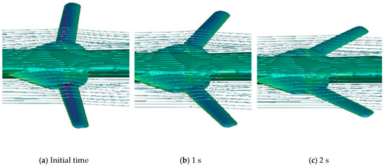
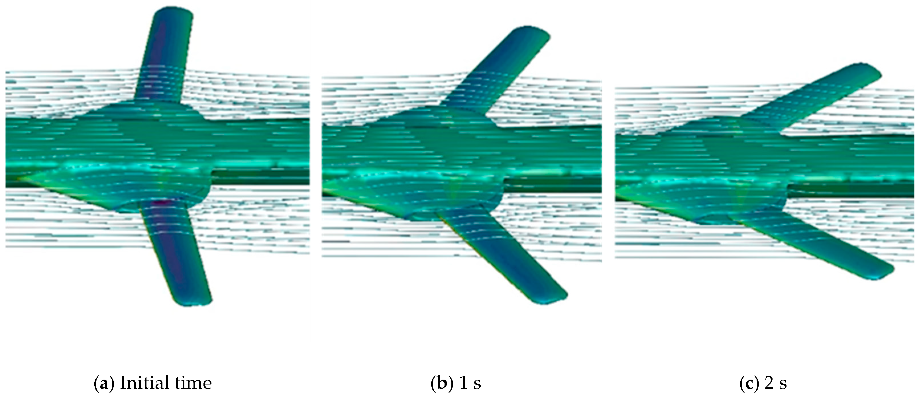
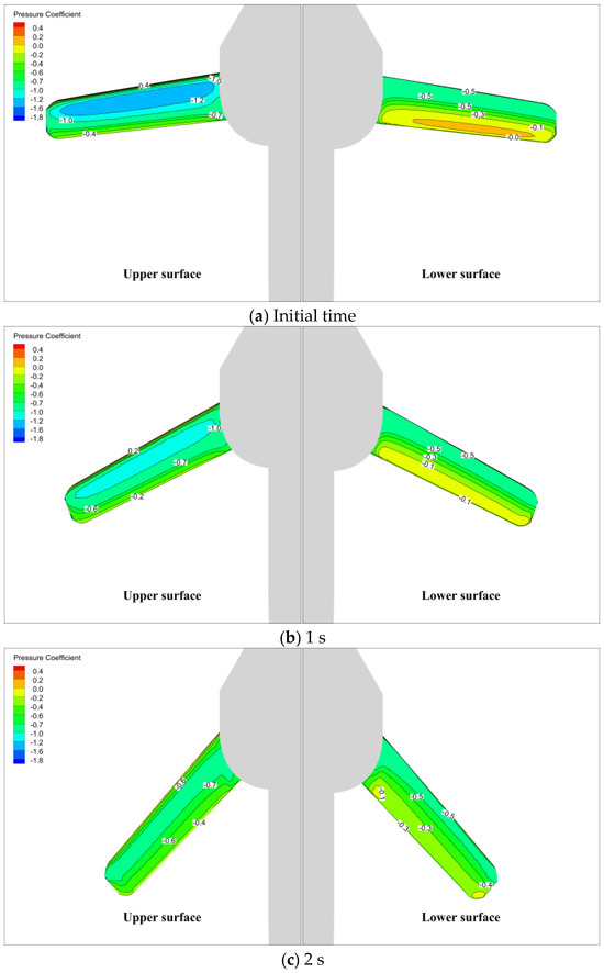
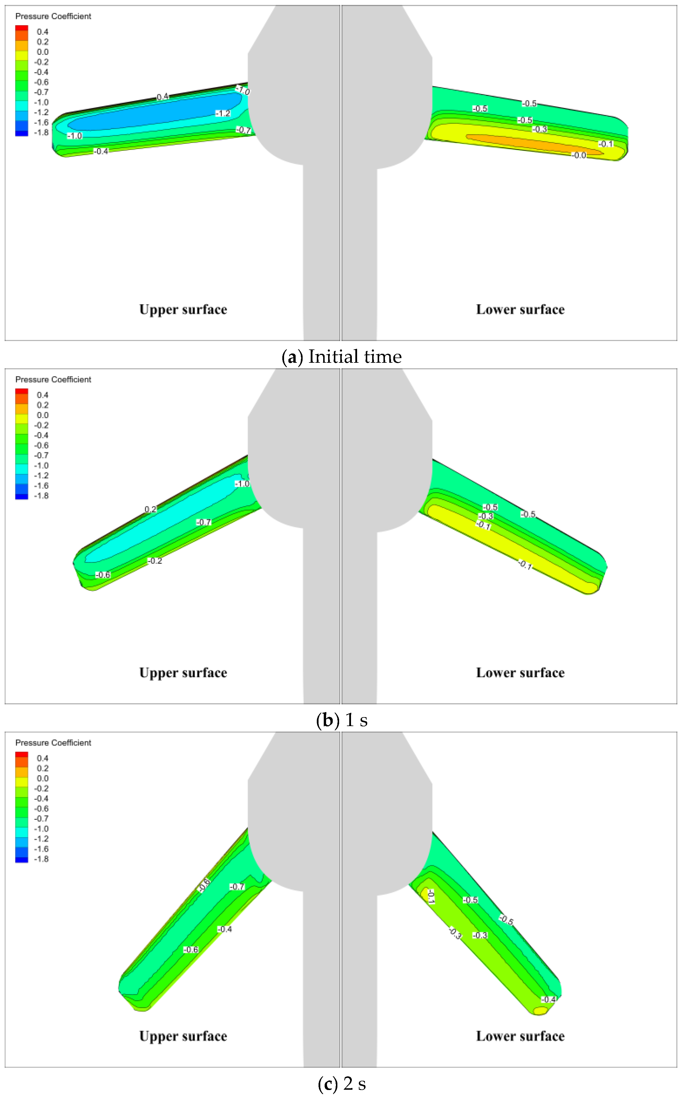
Figure 26 shows the pressure contours and streamlines near the morphing wing at 1 s and 2 s. Figure 27 presents the pressure coefficient distributions on the upper surface (left) and lower surface (right) in the initial state, as well as at 1 s and 2 s. From these results, it can be observed that as the sweep angle of the outer wing section increases, both the extent and intensity of the low-pressure region near the leading edge on the upper surface decrease. Meanwhile, the extent and intensity of the high-pressure region near the trailing edge on the lower surface are also reduced. This indicates that an increase in sweep angle leads to a reduction in lift generated by the wing, which is consistent with the trends observed in the lift coefficient curves.

Figure 26. Pressure distribution contours and streamlines during the deformation process.

Figure 27. Pressure coefficient contours of the upper surface (left) and lower surface (right) with increasing sweep angle.

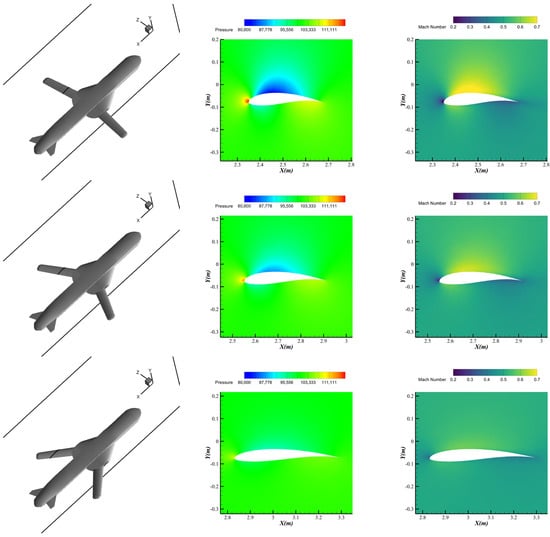
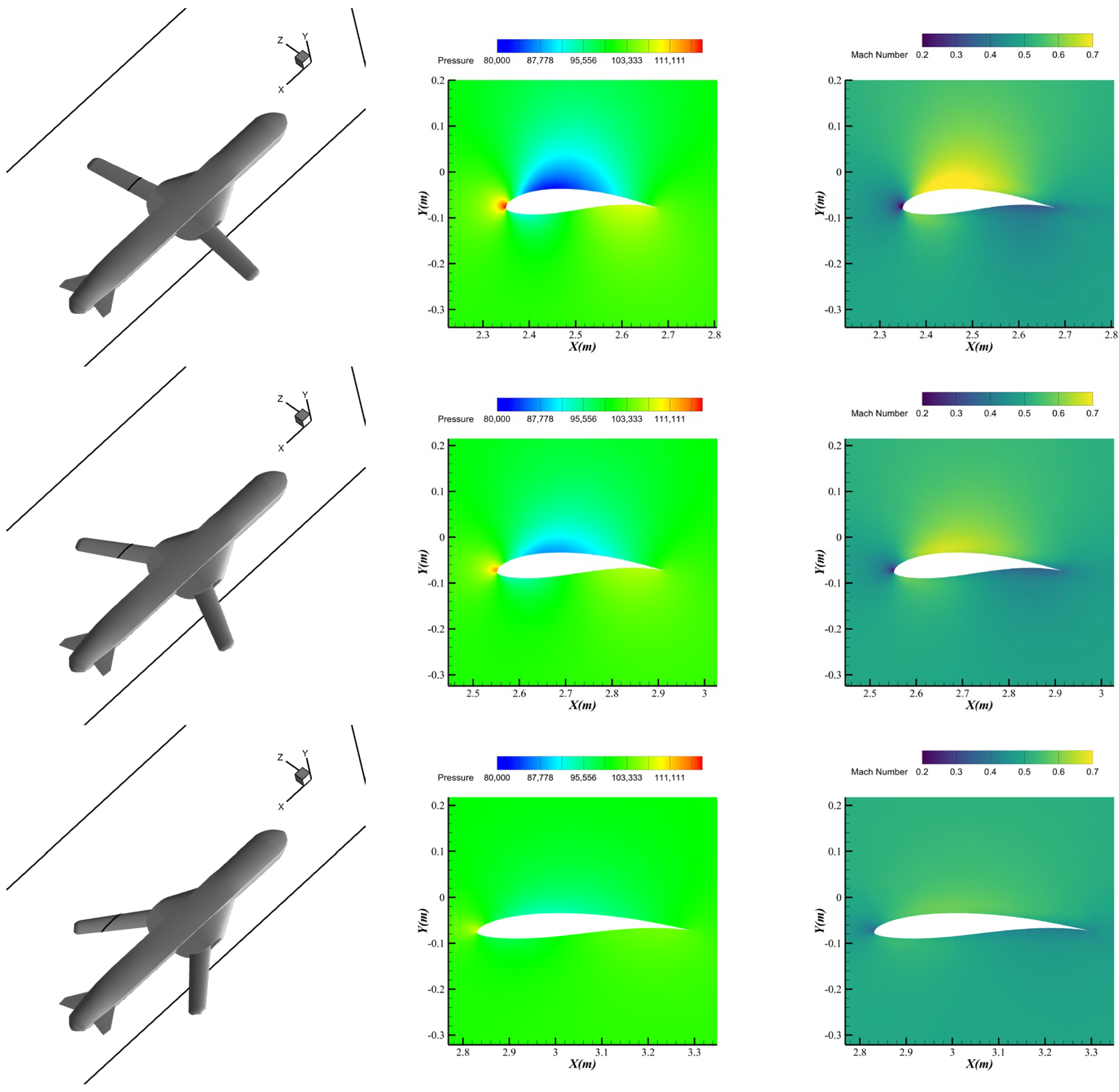
Figure 28 presents the pressure contours and Mach number distributions at the same sectional location under different sweep angles. The temporal evolution of the pressure and Mach fields reveals the dynamic mechanism of fluid–structure interaction during the continuous variable-sweep process. As the wing transitions from a small sweep angle to a larger one, a significant redistribution of aerodynamic loads is observed. Specifically, the suction peak on the upper surface gradually shifts downstream while its magnitude decreases. This trend is consistently reflected in the Mach number field, where the region of maximum acceleration moves along the chordwise direction with a slight reduction in intensity, indicating a decrease in effective camber and lift-generating capability.

Figure 28. Pressure and Mach number contours in the same section under different sweep angles.

6. Conclusions

A numerical framework for fluid–structure interaction (FSI) involving multibody structures is proposed in this study. The accuracy and capability of the proposed framework are validated through a combination of benchmark model verification and numerical simulations. The main conclusions can be summarized as follows:

The numerical results of the benchmark FSI model show good agreement with reference data, demonstrating that the proposed computational framework possesses satisfactory accuracy. The case study of a multibody flexible beam system connected by hinges further illustrates the capability of the method in simulating FSI problems involving flexible multibody structures.

For hinged multibody flexible-beam systems, the results indicate that the hinge location has a significant influence on the fluid–structure interaction characteristics of the multibody system. By analyzing the generation and evolution of flow vortical structures, it is found that the structural motion modes are closely related to the beam segment that is first affected by the vortices shed from the upstream cylinder. When $\phi$ is 0.625, the amplitude of displacement in the y-direction at point A is the largest, and when $\phi$ is 0.375, the amplitude of the displacement is the smallest.

Numerical simulations of a three-dimensional continuously variable-sweep wing showed that the aerodynamic coefficients decreased as the sweep angle increased. The increase in sweep angle gradually smoothed the pressure distribution over the wing surface, thereby reducing lift. In addition, aerodynamic loading induced sustained oscillations of the flexible wing, with a maximum wingtip amplitude of 0.053 m. Although the angle of attack varied at a constant rate, the aerodynamic loads continued to excite structural vibrations in the flexible wing, which in turn gave rise to time-dependent aerodynamic responses.

The method presented in this paper provides an effective approach for high-fidelity numerical simulation of the dynamic behavior of rigid–flexible coupled multibody morphing aircraft. Future work will extend the framework through efficient local RBF schemes for non-uniform meshes, immersed boundary coupling for complex deformations.

7. Scope and Limitations

This study employs a global Radial basis function (RBF) method to transfer data across the fluid–structure interface. However, for multibody systems with a large number of nodes, global RBF interpolation incurs substantial computational cost. Future work should therefore investigate compactly supported interpolation functions and adaptive local support domains to improve RBF interpolation accuracy on non-uniform meshes.

Moreover, the current implementation is limited by the capability of the dynamic-mesh deformation method and is therefore difficult to apply to cases involving complex deformations. Because the immersed boundary method can accommodate interfaces undergoing complex deformations, coupling it with the current fluid solver represents an important direction for addressing such problems.

References

- Xu, W.; Shen, L.; Peng, S.; Zhou, Y. Aerodynamics of a three-dimensionally deformed rigid wing. Int. J. Heat Fluid Flow 2024, 110, 109577. [Google Scholar] [CrossRef] [Scilit]
- Kamliya Jawahar, H.; Vemuri, S.S.; Azarpeyvand, M. Aerodynamic noise characteristics of airfoils with morphed trailing edges. Int. J. Heat Fluid Flow 2022, 93, 108892. [Google Scholar] [CrossRef] [Scilit]
- Sooraj, P.; Sharma, A.; Agrawal, A. Dynamics of co-rotating vortices in a flow around a bio-inspired corrugated airfoil. Int. J. Heat Fluid Flow 2020, 84, 108603. [Google Scholar] [CrossRef] [Scilit]
- Li, D.; Zhao, S.; Da Ronch, A.; Xiang, J.; Drofelnik, J.; Li, Y.; Zhang, L.; Wu, Y.; Kintscher, M.; Monner, H.P.; et al. A review of modelling and analysis of morphing wings. Prog. Aerosp. Sci. 2018, 100, 46–62. [Google Scholar] [CrossRef] [Scilit]
- Chu, L.; Li, Q.; Gu, F.; Du, X.; He, Y.; Deng, Y. Design, modeling, and control of morphing aircraft: A review. Chin. J. Aeronaut. 2022, 35, 220–246. [Google Scholar] [CrossRef] [Scilit]
- Parancheerivilakkathil, M.S.; Pilakkadan, J.S.; Ajaj, R.M.; Amoozgar, M.; Asadi, D.; Zweiri, Y.; Friswell, M.I. A review of control strategies used for morphing aircraft applications. Chin. J. Aeronaut. 2024, 37, 436–463. [Google Scholar] [CrossRef] [Scilit]
- Mowla, M.N.; Asadi, D.; Durhasan, T.; Jafari, J.R.; Amoozgar, M. Recent advancements in morphing applications: Architecture, artificial intelligence integration, challenges, and future trends—A comprehensive survey. Aerosp. Sci. Technol. 2025, 161, 110102. [Google Scholar] [CrossRef] [Scilit]
- Ajaj, R.M.; Parancheerivilakkathil, M.S.; Amoozgar, M.; Friswell, M.I.; Cantwell, W.J. Recent developments in the aeroelasticity of morphing aircraft. Prog. Aerosp. Sci. 2021, 120, 100682. [Google Scholar] [CrossRef] [Scilit]
- Zhu, J.; Yang, J.; Zhang, W.; Gu, X.; Zhou, H. Design and applications of morphing aircraft and their structures. Front. Mech. Eng. 2023, 18, 34. [Google Scholar] [CrossRef] [Scilit]
- Servetti, G.; Cestino, E.; Frulla, G. Parametric Evaluation of Morphed Wing Effectiveness. Aerospace 2026, 13, 187. [Google Scholar] [CrossRef] [Scilit]
- Luo, B.; Wei, L. Mechanical intelligence for artificial wings: A philosophy for multifold high-degree morphing with its mechanisms analogous to biology. Innovation 2026, 7, 101251. [Google Scholar] [CrossRef] [Scilit] [PubMed]
- Yang, J.; Zhang, Y.; Gu, X.; Li, J.; Fang, P.; Yang, X.; Wang, J.; Zhu, J.; Zhang, W. Bi-direction and flexible multi-mode morphing wing based on antagonistic SMA wire actuators. Chin. J. Aeronaut. 2024, 37, 373–387. [Google Scholar] [CrossRef] [Scilit]
- Tian, D.; Zhang, J.; Jin, L.; Huang, X. Design and research of a new multi-loop closed-chain morphing wing mechanism. Mech. Mach. Theory 2024, 199, 105697. [Google Scholar] [CrossRef] [Scilit]
- Zhang, J.; Liu, L.; Zhang, D.; Zhu, J.; Zhang, W. An intelligent, flexible morphing wing with posture-locking capability for cooperative and integral bending deformation. Cell Rep. Phys. Sci. 2026, 7, 103108. [Google Scholar] [CrossRef] [Scilit]
- Zheng, K.; Li, D.; Kan, Z.; Ma, K.; Wang, Z.; Zhang, L.; Xiang, J. Design and aerodynamic characteristic analysis of flexible morphing wing based on cellular structure. Chin. J. Aeronaut. 2025, 38, 103572. [Google Scholar] [CrossRef] [Scilit]
- Ozbek, E.; Ekici, S.; Karakoç, T.H. A comprehensive review of state-of-art FishBAC–fishbone active camber morphing wing surfaces–: A promising morphing method. Aircr. Eng. Aerosp. Technol. 2024, 96, 983–993. [Google Scholar] [CrossRef] [Scilit]
- Zhu, X.; Zhang, J.; Chen, W.; Gu, H. Tension-twist coupling morphing wing using a novel mechanical metamaterial. Aerosp. Sci. Technol. 2024, 155, 10974. [Google Scholar] [CrossRef] [Scilit]
- Cheng, G.; Ma, T.; Yang, J.; Chang, N.; Zhou, X. Design and Experiment of a Seamless Morphing Trailing Edge. Aerospace 2023, 10, 282. [Google Scholar] [CrossRef] [Scilit]
- Shi, X.; Yang, Y.; Wang, Z.; Zhang, S.; Sun, X.; Feng, W. Design and Shape Monitoring of a Morphing Wing Trailing Edge. Aerospace 2023, 10, 127. [Google Scholar] [CrossRef] [Scilit]
- Kilian, L.; Shahid, F.; Zhao, J.-S.; Nayeri, C.N. Bioinspired morphing wings: Mechanical design and wind tunnel experiments. Bioinspir. Biomim. 2022, 17, 046019. [Google Scholar] [CrossRef] [Scilit]
- Yang, H.; Jiang, S.; Wang, Y.; Xiao, H. Design, kinematic and fluid-structure interaction analysis of a morphing wing. Aerosp. Sci. Technol. 2023, 143, 108721. [Google Scholar] [CrossRef] [Scilit]
- Yang, S.; Xu, P.; Li, B. Design and rigid-flexible dynamic analysis of a morphing wing eight-bar mechanism. Nonlinear Dyn. 2024, 112, 15025–15060. [Google Scholar] [CrossRef] [Scilit]
- Preston, B.; Fasel, U.; Palacios, R.; Castrichini, A. Multibody Simulation of Flexible Aircraft with Variable-Sweep Wingtips. AIAA J. 2026, 64, 955–968. [Google Scholar] [CrossRef] [Scilit]
- Hua, S.; Wang, X.; Wang, Z. Rigid–Elastic Coupling Dynamics of Morphing Wing Aircraft. Aerospace 2025, 12, 327. [Google Scholar] [CrossRef] [Scilit]
- Riskin, D.K.; Willis, D.J.; Iriarte-Díaz, J.; Hedrick, T.L.; Kostandov, M.; Chen, J.; Laidlaw, D.H.; Breuer, K.S.; Swartz, S.M. Quantifying the complexity of bat wing kinematics. J. Theor. Biol. 2008, 254, 604–615. [Google Scholar] [CrossRef] [Scilit] [PubMed]
- Ye, K.; Yang, M.; Qin, L.; Xue, R.; Ye, Z. Effects of structural geometric nonlinearities on the transonic aeroelastic characteristics of wing. Aerosp. Sci. Technol. 2024, 149, 109161. [Google Scholar] [CrossRef] [Scilit]
- Grifò, A.; Ronch, A.D.; Benedetti, I. A computational aeroelastic framework based on high-order structural models and high-fidelity aerodynamics. Aerosp. Sci. Technol. 2022, 132, 108069. [Google Scholar]
- Zhang, C.; Guo, H.; Yu, L.; Lv, B.; Xia, H. Geometrically nonlinear flutter analysis based on CFD/CSD methods and wind tunnel experimental verification. CMES-Comput. Model. Eng. Sci. 2023, 136, 1743–1758. [Google Scholar] [CrossRef] [Scilit]
- Wang, J.; Li, J.; Lei, S.; Ren, Z.; He, Y. Geometric nonlinear static aeroelastic characteristics analysis of high-aspect-ratio wing with large deformation. Int. J. Aeronaut. Space Sci. 2022, 23, 315–325. [Google Scholar] [CrossRef] [Scilit]
- Li, K.; Kou, J.; Zhang, W. Aeroelastic reduced-order modeling for efficient static aeroelastic analysis considering geometric nonlinearity. J. Fluids Struct. 2024, 124, 104055. [Google Scholar] [CrossRef] [Scilit]
- Eldredge, J.D. Dynamically coupled fluid-body interactions in vorticity-based numerical simulations. J. Comput. Phys. 2008, 227, 9170–9194. [Google Scholar] [CrossRef] [Scilit]
- Wang, C.; Liu, Y.; Xu, D.; Wang, S. Aerodynamic performance of a bio-inspired flapping wing with local sweep morphing. Phys. Fluids 2022, 34, 051903. [Google Scholar] [CrossRef] [Scilit]
- Li, R.; Xiao, Q.; Liu, Y.; Hu, J.; Li, L.; Li, G.; Liu, H.; Hu, K.; Wen, L. A multi-body dynamics based numerical modelling tool for solving aquatic biomimetic problems. Bioinspir. Biomim. 2018, 13, 056001. [Google Scholar] [CrossRef] [Scilit] [PubMed]
- Le, V.D.T.; Nguyen, A.T.; Dang, N.T. Multibody-Dynamics Approach to Study the Deformation and Aerodynamics of an Insect Wing. AIAA J. 2023, 61, 2500–2516. [Google Scholar] [CrossRef] [Scilit]
- Cheng, K.C.-W.; Cea, A.; Palacios, R.; Castrichini, A.; Wilson, T. Nonlinear Multibody Modeling of Flexible Aircraft with Flared Hinged Wingtips. J. Aircr. 2025, 62, 929–948. [Google Scholar] [CrossRef] [Scilit]
- Han, J.; Wu, Z.; Yang, C. Nonlinear aeroelastic response analysis of wing with flared folding wingtip. J. Aerosp. Eng. 2024, 37, 04024013. [Google Scholar] [CrossRef] [Scilit]
- Joshi, V.; Jaiman, R.K.; Ollivier-Gooch, C. A variational flexible multibody formulation for partitioned fluid-structure interaction: Application to bat-inspired drones and unmanned air-vehicles. Comput. Math. Appl. 2020, 80, 2707–2737. [Google Scholar] [CrossRef] [Scilit]
- Masarati, P.; Morandini, M.; Mantegazza, P. An efficient formulation for general-purpose multibody/multiphysics analysis. J. Comput. Nonlinear Dyn. 2014, 9, 041001. [Google Scholar] [CrossRef] [Scilit]
- Turek, S.; Hron, J. Proposal for numerical benchmarking of fluid-structure interaction between an elastic object and laminar incompressible flow. In Fluid-Structure Interaction; Springer: Berlin/Heidelberg, Germany, 2006; pp. 371–385. [Google Scholar]
- Turek, S.; Hron, J.; Razzaq, M.; Wobker, H.; Schäfer, M. Numerical benchmarking of fluid-structure interaction: A comparison of different discretization and solution approaches. In Fluid Structure Interaction II; Springer: Berlin/Heidelberg, Germany, 2011; pp. 413–424. [Google Scholar]
- Ghiringhelli, G.L.; Masarati, P.; Mantegazza, P. Multibody implementation of finite volume C beams. AIAA J. 2000, 38, 131–138. [Google Scholar] [CrossRef] [Scilit]
- Tian, F.-B.; Dai, H.; Luo, H.; Doyle, J.F.; Rousseau, B. Fluid–structure interaction involving large deformations: 3D simulations and applications to biological systems. J. Comput. Phys. 2014, 258, 451–469. [Google Scholar] [CrossRef] [Scilit]
- Blevins, R.D.; Plunkett, R. Formulas for natural frequency and mode shape. J. Appl. Mech. 1980, 47, 461–462. [Google Scholar] [CrossRef] [Scilit]
- Weaver, W., Jr.; Timoshenko, S.P.; Young, D.H. Vibration Problems in Engineering; John Wiley & Sons: Hoboken, NJ, USA, 1991. [Google Scholar]
- Williamson, C.H.K.; Brown, G.L. A series in 1/√re to represent the strouhal–reynolds number relationship of the cylinder wake. J. Fluids Struct. 1998, 12, 1073–1085. [Google Scholar] [CrossRef] [Scilit]
Disclaimer/Publisher’s Note: The statements, opinions and data contained in all publications are solely those of the individual author(s) and contributor(s) and not of MDPI and/or the editor(s). MDPI and/or the editor(s) disclaim responsibility for any injury to people or property resulting from any ideas, methods, instructions or products referred to in the content. |
© 2026 by the authors. Licensee MDPI, Basel, Switzerland. This article is an open access article distributed under the terms and conditions of the Creative Commons Attribution (CC BY) license.