


Abstract
Reliable launch environment recognition is essential for assisted-takeoff unmanned aerial vehicles (UAVs) because it determines the timing of flight-control activation, motor startup, and mode switching. However, recognition parameters are commonly selected empirically, and their effects on failure rate are rarely quantified. This study proposes a failure-rate-oriented parameter optimization framework integrating Monte Carlo failure-rate modeling, Sobol global sensitivity analysis, and particle swarm optimization (PSO) for UAV launch environment recognition. Three parameters in the sliding-window logic, namely the acceleration threshold , number of sampling points within the judgment window , and threshold-reaching proportion , are analyzed and optimized under low-overload catapult-launch and high-overload gun-launch conditions. Sobol analysis identifies both individual contributions and interaction effects, providing interpretable guidance for parameter design, while PSO searches for parameter combinations that minimize the recognition failure rate. An additional multi-objective optimization was conducted by incorporating recognition delay, false-trigger probability, and sampling frequency to evaluate the trade-off between recognition reliability and response speed. Results showed that dominated the low-overload case, contributing 54.88%, whereas dominated the high-overload case, contributing 37.06%. PSO reduced the upper limit of the 95% confidence interval of the failure rate by 88.47% and 90.22%, respectively. The multi-objective optimization further reduced the mean recognition delay from 55.8 ms to 45.5 ms under the low-overload condition and from 8.8 ms to 4.1 ms under the high-overload condition while maintaining low false-trigger probability and recognition failure rate. Experimental tests verified successful recognition in six low-overload and six high-overload launches. Runtime comparisons with genetic algorithm (GA), differential evolution (DE), and random search (RS) further demonstrated the offline computational efficiency of PSO.
1. Introduction
Unmanned aerial vehicles (UAVs) have been widely used in both civil and military applications because of their flexibility, rapid deployment capability, and low operational cost [1,2,3]. In civil scenarios, UAVs are commonly employed for emergency rescue, disaster assessment, agricultural monitoring and geographic surveying, where rapid deployment from confined or unprepared sites is often required. In military scenarios, UAVs are increasingly used for reconnaissance, surveillance, communication, target indication, and other time-sensitive missions, in which vehicle-mounted, shipborne, catapult-assisted, tube-launched, or gun-launched deployment may be adopted to improve launch flexibility and mission responsiveness. Unlike conventional runway takeoff, these assisted-launch modes usually generate transient acceleration overloads with different amplitudes, durations, and noise characteristics. The onboard system must correctly identify the launch environment to determine the proper timing for flight-control activation, motor startup, and mode switching. Therefore, reliable launch environment recognition is a safety-critical function directly related to launch success, flight stability, and mission execution.
However, improper selection of environment feature recognition parameters directly affects recognition accuracy, leading to an increased failure rate, abnormal motor startup or control commands, and even crashes. Therefore, conducting sensitivity analysis and optimization research on environment feature recognition parameters is of great theoretical significance and engineering value for ensuring accurate launch environment recognition and flight safety of UAVs.
The launch environment feature recognition method and its parameter selection are crucial to the accuracy and safety of UAV launch environment recognition. Wang et al. [4] employed Binary Decision Diagrams and a Multi-Objective Quantum Particle Swarm Optimization method to establish a reliability model for multi-phase missions of UAV swarms. They found that accurate recognition of the launch environment is critical for ensuring ground communication during the launch phase, thereby directly guaranteeing reliable autonomous control in subsequent flight and combat phases. Zhang et al. [5] proposed a novel hydrodynamic catapult scheme for UAVs, analyzed the dynamic characteristics of the catapult, and presented the resulting launch thrust profile. Lv et al. [6] used the peak impact force and its duration as launch environment recognition parameters and applied them to an inertial switch, verifying the contact performance of the switch through simulation. Qin et al. [7] employed a 1500 g acceleration overload as the characteristic parameter for launch environment recognition, and validated the reliability of the recognition method under launch conditions through finite element simulation and tests. Nie et al. [8] adopted the acceleration amplitude and pulse duration during launch for launch environment recognition. Based on this recognition method, they investigated the response characteristics of a MEMS inertial electrical switch through dynamic simulation. Wang et al. [9] proposed a “single threshold + time window” method for launch environment recognition. This method used an acceleration sensor to identify launch overload and set parameters based on experience. It determined whether the time interval between two overload events exceeding the threshold falls within a preset time window. However, this method only relied on a single overload sampling point, making it difficult to effectively filter out abnormal overload signals. Yin et al. [10,11] further proposed a “dual-threshold + time window” method. This method increased the number of sampling points and time windows from one to two, simultaneously judging whether the time intervals for both overload events exceeding their thresholds meet the requirements of their respective time windows. Nevertheless, this method still struggled to effectively filter out and correctly identify interfering signals such as spike noise.
In the aforementioned studies, parameter selection was largely empirical, merely fulfilling the basic function of environment recognition. However, these studies failed to establish a correlation between parameters and the recognition failure rate, and were unable to assess the safety of environment recognition under large-sample conditions. Furthermore, the degree of influence of each parameter on the failure rate remained unclear, and a systematic theoretical analysis was lacking, making it difficult to quantitatively study the impact of recognition parameters on the safety failure rate.
Sensitivity analysis is an effective method capable of identifying key parameters that have a significant impact on model output [12,13]. Sensitivity analysis methods are mainly divided into global methods and local methods [14,15]. Global methods include variance-based methods and screening methods; local methods are represented by the One-At-a-Time (OAT) method. Among the various global methods, the Sobol method is a widely used variance-based sensitivity analysis technique. Currently, sensitivity analysis methods have been successfully applied in many engineering fields to analyze the influence of input parameters on the objective function. Pan et al. [16] proposed a non-destructive parameter identification method. They utilized the whale optimization algorithm with global search capability to identify parameters of an electrochemical model, and employed the OAT method to analyze the sensitivity of key parameters of the battery model. Ultimately, they determined that the electrode-related lithium-ion transport parameters were the key factors determining calculation accuracy. Li et al. [17] established a reliability and local sensitivity analysis framework for defective bearings, revealed the evolution pattern of failure probability with respect to defect size, and determined the key ranking of influencing factors. Liu et al. [18] proposed a novel metaheuristic algorithm called Puma Optimizer (PO) and applied it to parameter identification for various proton exchange membrane fuel cells (PEMFC) systems. They conducted sensitivity analysis using the OAT method and identified the key factors affecting the performance of PEMFC systems. However, the aforementioned single-factor sensitivity analysis methods can only examine the impact of varying a single parameter on the output, and fail to reveal the effects of coupling interactions among parameters. When strong interactions exist among parameters, the OAT method may not accurately reflect the true sensitivity of the parameters.
The Sobol method is a variance-based global sensitivity analysis technique. It can not only quantify the contribution of a single parameter to the output variance (main effect) but also evaluate the contribution of interactions among parameters to the output variance (interaction effects), thereby comprehensively revealing the complex relationships among parameters [19,20,21]. Chen et al. [22] combined the Sobol algorithm with an Adaptive Neuro-Fuzzy Inference System (ANFIS) to analyze factors influencing the impact point dispersion of small-caliber spin-stabilized projectiles, and identified mass eccentricity, moment of inertia, and projectile mass as significant influencing factors. Ge et al. [23] applied the Sobol method to identify key design parameters that significantly influence the modal characteristics of an airship. The research results indicated that the airship’s length and fineness ratio have a significant impact on its stable modes. Ma et al. [24] comprehensively applied single-parameter and Sobol multi-parameter sensitivity analysis methods to systematically evaluate the sensitivity of airship thermal parameters (e.g., absorptivity, emissivity) and structural parameters (e.g., elastic modulus, thickness) on the coupling effect, and examined the independent and synergistic effects of these parameters. Hou et al. [25] identified parameters with significant influence on the heat transfer characteristics of aviation gears through Sobol global sensitivity analysis. The study pointed out that gear speed, oil supply flow rate, and their synergistic effects play a dominant role in the heat transfer characteristics. Through numerical simulation and experimental research, Li et al. [26,27] quantified the influence of operating conditions, structural parameters, and friction coefficient on the three-dimensional temperature field distribution of gears, and conducted a comparative analysis of the thermal sensitivity of each parameter. Tu et al. [28], based on experience, identified the weak links of a latching mechanism. They combined probabilistic algorithms, the Kriging surrogate model, and finite element simulation to quantify the impact of input uncertainty on the mechanism’s response. They then used the First-Order Reliability Method (FORM) for reliability and sensitivity calculations, and finally proposed corresponding improvement measures.
In summary, global sensitivity analysis, as an effective tool for assessing the importance of parameters in complex systems, has been successfully applied in many engineering fields such as battery management, parameter identification, airship design, and gear transmission. However, in the field of UAV launch environment recognition and safety control, research on the sensitivity analysis of environment feature recognition parameters remains relatively limited. Existing work is mostly based on single-factor analysis, and parameter selection largely relies on experience, lacking systematic quantitative research on multi-parameter coupling effects. Particularly in a dynamic launch environment, the interaction among environment feature recognition parameters and their influence mechanism on the failure rate remain unclear.
To address these challenges, this paper aims to analyze the sensitivity of UAV launch environment feature recognition parameters, seek their optimal combination, and ultimately provide a systematic and quantitative approach for parameter optimization. The main contributions of this paper are summarized as follows:
(1) Existing studies on UAV launch environment feature recognition methods [4,5,6,7,8,9,10,11] only achieved the basic function of environment recognition, without establishing a correlation between the parameters and the recognition failure rate, and thus could not assess the safety of environment recognition under large-sample conditions. This paper establishes a correlation model between the parameters and the failure rate using the Monte Carlo method, not only effectively evaluating the safety of launch environment feature recognition but also providing a foundation for Sobol sensitivity analysis.
(2) In the study of sensitivity analysis [22,23,24,25,26,27,28], applications related to UAV launch environment feature parameter recognition remain relatively limited. The influence of each parameter on the failure rate remains unclear, and systematic theoretical analysis is lacking, making it difficult to quantitatively study the impact of recognition parameters on the failure rate. This paper employs Sobol global sensitivity analysis based on the sliding time window environment feature recognition method to quantify the influence of each parameter on the recognition failure rate and reveal their interaction effects.
(3) To address the issue that the selection of recognition parameters largely relies on experience, this paper, based on the sensitivity analysis, employs the particle swarm optimization (PSO) algorithm to optimize the parameters, focusing on those with high sensitivity and strong interaction effects. The optimal parameter combination was obtained, and the optimization results were validated through UAV launch tests.
(4) To address the practical requirements of rapid recognition and false-trigger suppression, this study further develops an additional multi-objective optimization model. In this model, recognition delay, false-trigger probability, and recognition failure rate are simultaneously considered, and the sampling frequency is introduced as an additional design variable. This extension evaluates the trade-off between recognition reliability and response speed and improves the practical applicability of the proposed framework.
(5) To demonstrate the generalizability of the proposed optimization method, this study further applies it to a high-overload gun-launched UAV environment (peak overload 11,000 g). Using the same global sensitivity analysis and PSO procedure, the optimal parameter combination under high-overload conditions was obtained and validated through tests. By comparing with the optimal parameter combination under UAV low-overload conditions, the results show that the method significantly reduces the failure rate under both low-overload and high-overload launch conditions, thereby demonstrating the scalability and robustness of the proposed approach. This study is expected to provide a theoretical basis and engineering guidance for the optimal design of UAV launch environment feature recognition parameters.
The remainder of this paper is organized as follows. Section 2 presents the launch environment feature recognition method and establishes the Monte Carlo-based failure-rate model. Section 3 conducts Sobol global sensitivity analysis under low-overload and high-overload launch conditions. Section 4 presents the PSO-based parameter optimization, additional multi-objective optimization considering recognition delay and false-trigger probability, computational complexity analysis, and comparison with alternative optimization algorithms. Section 5 verifies the optimized parameters through low-overload and high-overload launch tests and discusses the applicability and limitations of the proposed framework. Finally, Section 6 summarizes the main conclusions.
Figure 1 illustrates the conceptual framework of the proposed approach. First, the launch environment characteristics are analyzed under two representative conditions, namely low-overload catapult launch and high-overload gun launch. Based on these characteristics, three key recognition parameters are defined: acceleration threshold , window size , and threshold-reaching ratio . Then, a Monte Carlo-based failure-rate model is established by combining the measured acceleration overload, recognition parameters, and Gaussian white noise. The resulting failure rate is used as the model input for Sobol global sensitivity analysis, which quantifies the main and interaction effects of the recognition parameters. Subsequently, PSO is employed to search for the optimal parameter combination within the feasible parameter ranges. Finally, the optimized parameters are implemented in the onboard environment information recognition module and verified through UAV launch tests.
Figure 1.
Framework of the proposed approach.
2. Launch Environment Feature Recognition Method and Failure Rate Model Establishment
This section presents the basic recognition logic and the failure-rate model used for parameter evaluation. Launch environment recognition is essentially a real-time decision process based on the measured acceleration signal. Therefore, the recognition parameters must be clearly defined before sensitivity analysis and optimization can be conducted. In this section, the sliding-window recognition method is first described, including the acceleration threshold, window size, and threshold-reaching proportion. Then, a Monte Carlo-based failure-rate model is established by considering measurement uncertainty and random disturbances in the acceleration signal. This model provides a quantitative objective for the subsequent sensitivity analysis and parameter optimization.
2.1. Launch Environment Feature Recognition Method
The launch environment studied in this paper refers to the thrust from the launch platform that a UAV experiences at the moment of launch. In this environment, the UAV’s onboard system utilizes the acceleration information generated during launch to perform environment recognition according to a preset logic, and outputs a recognition signal to switch the flight control mode, thereby ensuring flight safety and reliable mission completion. The environment feature recognition method adopted in this paper involves three key parameters: the acceleration threshold (), the number of sampling points within the time judgment window T (ns), and the proportion of sampling points that reach the acceleration threshold (r). These three parameters collectively constitute a comprehensive criterion for the UAV to extract features, make status judgments, and arrive at a recognition decision from the dynamic launch environment. determines the system’s sensitivity to launch overload and is used to distinguish the genuine launch signal from other low-amplitude disturbances. represents the number of sampling points involved in the statistics within the time window, directly influencing the algorithm’s ability to suppress transient noise and its response speed for status judgment. r is used to ensure the continuity and stability of the overload, preventing false triggering caused by a single noise spike.
The launch overload is sampled periodically. The latest acceleration value obtained from each sampling replaces the oldest record within the time window, thereby achieving a sliding window. Within this sliding time window, if the latest sampled value exceeds the preset threshold , it is counted as a valid overload event. When the cumulative time proportion of valid overload events within the window reaches or exceeds the threshold r, the system determines that a launch overload has been recognized and outputs an environment recognition signal. Acceleration overload is an inherent and directly measurable motion characteristic of launch munitions for platforms such as UAVs. Therefore, the environment feature recognition method proposed in this paper has direct applicability and universal reference value for the design of launch environment recognition logic for UAVs employing this type of launch method.
The principle of the environment feature recognition method is illustrated in Figure 2. Assume the sampling frequency of the acceleration overload is 1/T1, and the length of the sliding time window is T. Within one acquisition cycle, a total of ns points are collected in the window, and the sequence of overload values is stored as: a1, a2,……an, anew represents the most recently sampled overload value, and aold represents the oldest value in the current window that is about to be replaced. When the latest sampled value anew > ath, the count of valid points D increases by 1, i.e., D = D + 1; At the same time, if the oldest value being replaced, aold > ath, the count of valid points D should be decreased by 1 accordingly, i.e., D = D − 1. This update mechanism ensures that D can reflect the overload status within the current sliding window in real time and accurately. The process loops based on one acquisition cycle. At the end of each acquisition cycle, it checks whether the condition D/ns ≥ r holds true. If it holds, the system determines that a launch overload has been recognized.
Figure 2.
Principle of the launch environment feature recognition method. The horizontal dashed line denotes the acceleration threshold . The vertical dashed lines indicate the sampling instants, and the interval between two adjacent vertical dashed lines represents the sampling period .
The process of launch environment feature recognition is shown in Figure 3. First, preset the parameters: ath, ns, r. After the system starts, sampling is performed through the sliding time window. In each update cycle, the number of valid points D that have reached the threshold ath within the current window is evaluated. If D/ns ≥ r, it determines that a launch overload has been recognized and outputs an environment recognition signal; otherwise, it continues to slide the window and repeats the judgment process above.
Figure 3.
Flowchart of launch environment feature recognition.
2.2. Establishment of the Launch Environment Recognition Failure Rate Model
The launch environment recognition failure rate is defined as the probability that the UAV’s onboard system fails to correctly output an environment recognition signal under given launch conditions. In an actual launch process, the measured acceleration overload is often superimposed with various noises, such as inherent sensor noise, environmental disturbances, and mechanical vibrations from the catapult mechanism. To simulate this uncertainty, this paper models these noises as Gaussian white noise X~N(0, ơ2), where σ is the noise standard deviation. Based on the actual acceleration overload data measured during UAV launch, a large number of simulation experiments are conducted using the Monte Carlo method (each experiment is implemented by adding different noise). The proportion of experiments where the environment recognition signal is not output is then defined as the failure rate. The failure rate F is calculated as follows:
where F is the launch environment recognition failure rate, n is the number of simulations in which the environment recognition signal was not output, and N is the total number of Monte Carlo simulations.
2.3. Characterization of Different Launch Environments
To compare the performance of the proposed method under different launch environments, two typical launch environments are selected, as shown in Table 1: low-overload and high-overload launch environments. The low-overload data come from actual UAV catapult launch tests with a sampling frequency of 1 kHz. The high-overload data come from gun-launch tests with a sampling frequency of 40 kHz. Compared with the low-overload launch environment, the high-overload launch environment has a much higher peak acceleration but a significantly shorter duration. This short duration requires the environment recognition algorithm to have a faster response speed, thus requiring a higher sampling frequency to accurately capture the transient overload signal.
Table 1.
Characteristic parameters of different launch environments.
The proposed optimization framework combining Sobol global sensitivity analysis and the PSO method is inherently adaptable to both environments. Regardless of the overload magnitude or signal duration, the framework can systematically quantify the sensitivity of the failure rate to each recognition parameter (ath, ns, r) and search for the optimal parameter combination. The following sections will apply this framework to the two launch environments separately to demonstrate its scalability and robustness under low-overload and high-overload conditions.
2.4. Overall Procedure of the Proposed Framework Integrating Sobol Sensitivity Analysis and PSO
To make the proposed method more reproducible and easier to follow, the overall procedure of the Sobol-PSO-based parameter optimization framework is summarized in Algorithm 1. The procedure includes failure-rate modeling, global sensitivity analysis and offline parameter optimization. The same procedure is applied to both low-overload and high-overload launch conditions, while the acceleration data and feasible parameter ranges are defined according to the corresponding launch environment.
| Algorithm 1. Sobol-PSO-based parameter optimization framework. |
| Input: Measured launch acceleration signal ; parameter vector ; feasible parameter ranges ; Monte Carlo simulation number ; Sobol sample size ; PSO parameters, including swarm size and maximum iteration number . Output: Sobol sensitivity indices; optimized recognition parameters ; recognition failure rate. Step 1: Analyze the launch environment characteristics and determine the feasible ranges of , , and . Step 2: For a given parameter vector , generate noisy acceleration sequences by adding Gaussian white noise to the measured acceleration signal. Step 3: Apply the sliding-window recognition logic to each noisy acceleration sequence. If the proportion of samples exceeding in a window satisfies , the launch environment is recognized successfully. Step 4: Repeat Step 2 and Step 3 for Monte Carlo simulations and calculate the recognition failure rate . Step 5: Generate Sobol sampling matrices within the feasible parameter ranges and evaluate for all Sobol samples. Step 6: Calculate the first-order, total-order, and interaction sensitivity indices to quantify the effects of , , and on the recognition failure rate. Step 7: Initialize the PSO population within the feasible parameter ranges and evaluate the fitness value of each particle. Step 8: Update the particle velocity, particle position, individual best position, and global best position until the maximum iteration number is reached. Step 9: Select the global best particle as the optimized parameter combination . |
3. Sensitivity Analysis of Launch Environment Feature Recognition Parameters
Based on the recognition logic and failure-rate model established in Section 2, this section investigates how the key recognition parameters affect the recognition failure rate. Since the acceleration threshold, window size, and threshold-reaching proportion may influence the failure rate both individually and interactively, a global sensitivity analysis method is required rather than a one-factor-at-a-time analysis. Sobol sensitivity analysis is therefore adopted to quantify the first-order effects, total effects, and interaction effects of the three parameters. The analysis is performed separately for low-overload and high-overload launch conditions to reveal the parameter importance under different launch environments.
3.1. Analysis Method
The Sobol method is a variance-based global sensitivity analysis technique. It decomposes the total output variance into parts contributed by each input parameter and their interactions, generating a corresponding sensitivity index for each parameter, known as the Sobol index. This method can quantify the contribution of each input variable to the output variance, effectively distinguishing between the main effects and interaction effects of parameters, thereby comprehensively revealing the complex relationships among them. The sensitivity index reflects the relative strength of the influence of input parameter uncertainty on the model output.
The calculation formulas for Sobol indices of various orders are as follows:
where Si represents the first-order sensitivity of parameter i, measuring the contribution of a single input parameter to the output variance. Sij represents the second-order sensitivity, quantifying the contribution of the interaction between two parameters to the output variance; higher-order indices follow a similar pattern. V and Vis correspond to the total variance and the partial variances of the respective terms, respectively.
The total sensitivity of parameter i is defined as the sum of all sensitivity indices involving parameter i, and is expressed as:
STi is the total sensitivity index, measuring the contribution of the interactions between variable i and all other variables to the output variance.
The contribution rate of each parameter can be given by the following formula:
The higher-order sensitivity index of a parameter can be expressed as:
The higher-order proportion is expressed as:
The implementation steps of Sobol global sensitivity analysis are as follows:
(1) Define the model and parameter space. First, construct a computational model with the recognition failure rate as the objective function. Determine the number of parameters to be analyzed (dimension D), and set the value range and probability distribution for each parameter based on actual engineering constraints.
(2) Generate sampling matrices. Use the Sobol sequence for random sampling. Generate random samples within [0, 1] using the Sobol sequence, and map the sample data to the actual parameter range through a linear transformation (Parameter value range = min + Sobol sequence × (max − min)). Using this method, generate two input matrices, A and B, each of size N × D, where N is the number of samples, and D is the number of parameters.
(3) Construct the hybrid matrices ABi. Replace the i-th column of matrix A with the i-th column from matrix B to generate D hybrid matrices. This results in (D + 2) input matrices, each of size N × D.
(4) Calculate model outputs. Substitute these data into the corresponding failure rate calculation models to obtain the corresponding output matrix Y.
(5) Calculate sensitivity indices. Input the output matrices into the sensitivity index analysis formulas to solve for the main effect index Si (first-order effect index) and the total effect index STi for each parameter.
Here,
where N represents the total number of samples, j indicates the j-th sample, and i indicates the i-th parameter. Si is the first-order sensitivity of the parameter, describing the contribution of the random factor Xi “alone” to the total output variance. The larger the Si, the greater the influence of the uncertainty of Xi on the system’s output. STi is the total-order sensitivity, i.e., the sum of sensitivity indices of all orders for parameter Xi. When STi and Si for an input variable Xi differ significantly, it can be considered that the interactions between variable Xi and other input variables have a significant impact on the system output. Conversely, if they are close, it can be considered that the interaction effects are relatively small.
The above Sobol sensitivity analysis process is illustrated in Figure 4.
Figure 4.
Flowchart of Sobol sensitivity analysis. The blue dashed boxes indicate grouped steps within the same stage. The upper dashed box denotes the construction of the launch environment feature recognition method and the failure-rate model, whereas the middle dashed box denotes the generation of the input matrices and hybrid matrices for Sobol index calculation.
3.2. Sensitivity Analysis of Environment Feature Recognition Parameters Under Low Overload
3.2.1. Convergence Analysis Under the Low-Overload Environment
In failure rate analysis, the number of Monte Carlo simulations is a key factor affecting the accuracy of the results. An insufficient number of simulations may lead to significant statistical errors and computational bias. To determine the appropriate number of simulations to reduce uncertainty, a convergence analysis of the failure rate was conducted in this study. Figure 5 shows the failure rate convergence curve under the initial parameter combination (ath = 5.4, ns = 85, r = 80%) in the low-overload environment. It can be seen from Figure 5 that when the number of simulations is small, the failure rate fluctuates significantly. This indicates that an insufficient number of simulations introduces calculation errors, leading to a lack of statistical validity. As the number of simulations increases, the failure rate gradually stabilizes. When the number of simulations reaches 10,000, the failure rate has essentially converged. Therefore, the number of Monte Carlo simulations in this paper is set to 10,000 to ensure the statistical validity of subsequent analyses.
Figure 5.
Failure rate convergence curve under the low-overload environment.
The reliability of Sobol sensitivity analysis results is also affected by the sample size N. A sample size that is too small may lead to significant computational errors and statistical uncertainty, while an excessively large sample size would unnecessarily increase the computational cost [29,30,31]. To determine the appropriate sample size N, a convergence analysis of the Sobol method was conducted in this study, and the results are shown in Figure 6. Combined with the Sobol sensitivity analysis method described earlier, this analysis evaluated the trend of the total sensitivity index for each parameter and the sum of the three indices as the sample size increased. The convergence analysis indicated that when the sample size exceeded 1500, the total-order sensitivity indices of each parameter reached stable convergence. Therefore, a sample size of N = 1500 was chosen for the subsequent Sobol sensitivity analysis in this paper. This sample size is sufficient to ensure the statistical reliability of the sensitivity ranking and the accuracy of the parameter contribution assessment.
Figure 6.
Convergence analysis of the Sobol method under the low-overload environment.
3.2.2. Results and Discussion Under the Low-Overload Environment
The parameter ranges used in the Sobol sensitivity analysis were determined based on the measured launch acceleration characteristics, sampling frequency, overload duration, and the physical requirements for avoiding missed recognition and false triggering. Under the low-overload catapult-launch condition, the measured peak acceleration was approximately 15 g, and the overload duration was approximately 100 ms. Therefore, the acceleration threshold was selected as 5~8 g. This range is clearly higher than the pre-launch vibration and sensor noise levels observed in the measured data, while remaining lower than the main amplitude of the actual launch overload. Thus, it can reduce the risks of both false triggering and missed recognition. The sampling frequency of the low-overload test was 1 kHz. Accordingly, ~100 was used in the Sobol sensitivity analysis, corresponding to a time-window length of 10~100 ms. This range covers window lengths from rapid-response recognition to nearly the entire duration of the low-overload pulse. The threshold-reaching proportion was set to 50%~90% to reflect the trade-off between recognition speed and anti-interference capability. A lower is beneficial for improving response speed, but it may increase the risk of false triggering caused by transient spike disturbances. In contrast, a higher can improve recognition robustness, but may increase recognition delay or the probability of missed recognition.
The distribution types and parameter ranges are set, as shown in Table 2. The sample size for the Sobol analysis was 1500, and the number of Monte Carlo simulations for failure rate calculation was 10,000.
Table 2.
Parameter distribution types and ranges under the low-overload environment.
Figure 7 displays the first-order and total sensitivity indices for the launch environment feature recognition parameters. The first-order sensitivity characterizes the impact of a single parameter varying independently on the failure rate. Higher-order sensitivity quantifies the synergistic effect of multiple parameters interacting on the system response. The total sensitivity index comprehensively reflects the overall impact of the parameter itself and its interactions with other parameters.
Figure 7.
First-order and total sensitivity of the recognition parameters under the low-overload environment.
It can be observed from Figure 7 that the first-order sensitivity values for parameters ath, ns and r are 0.009, 0.416, and 0.114, respectively. Among them, parameter ns has the largest first-order sensitivity, indicating that its independent effect on the failure rate is the most significant. The independent effects of parameters ath and r are relatively small. The difference between the total and first-order sensitivity for parameter r is relatively large, at 0.315. This indicates that the interaction effects of this parameter with others have a significant influence on the failure rate. For the other two parameters (ath and ns), the differences between total and first-order sensitivity are 0.126 and 0.27, respectively, suggesting that the influence of their interaction effects on the output is relatively small. To further investigate the interactions among parameters, a heatmap of the second-order interaction effect indices is presented in Figure 8.
Figure 8.
Heatmap of second-order interaction effects under the low-overload environment.
In Figure 8, the darker the color of a block, the larger the corresponding second-order interaction effect index, meaning the stronger the influence of the interaction between the two parameters on the failure rate. It can be seen from the figure that the interaction effect indices for the pairs (ath, ns), (ath, r) and (ns, r) are relatively high, indicating that the interactions between these parameter pairs have an important impact on the failure rate. Among these, the interaction between ns and r is the most prominent, with an index as high as 0.194. This is because ns and r jointly determine the robustness and response speed of the environment feature recognition method. By balancing anti-interference capability and recognition sensitivity, they synergistically influence the final recognition failure rate. In comparison, the second-order sensitivity indices for the parameter pairs (ath, ns) and (ath, r) are 0.048 and 0.014, respectively, indicating a relatively smaller influence. Therefore, in the parameter optimization process, in addition to focusing on parameters with large total sensitivity, special attention should also be paid to the reasonable combination of ns and r to achieve better results.
The results of the global sensitivity analysis of the failure rate with respect to each parameter are summarized in Table 3. It can be seen that ns has the most significant impact on the UAV launch environment recognition failure rate, with a contribution rate of 54.88%. r is the secondary influencing factor, with a contribution rate of 34.32%; the impact of ath is the smallest, at only 10.80%. Furthermore, the average proportion of higher-order sensitivity terms in the total sensitivity for all parameters is 68.71%, indicating that synergistic effects among parameters have a significant influence on the recognition failure rate. Specifically, the higher-order proportion for ns is relatively small (39.36%), indicating that its independent contribution is dominant. In contrast, the higher-order proportions for ath and r are as high as 93.33% and 73.43%, respectively, indicating that their synergistic effects are dominant. This finding reveals significant differences in the mechanisms of action among the different parameters. Therefore, when conducting parameter optimization design, the synergistic effects among parameters must be taken into consideration. The sensitivity analysis above not only quantifies the influence of each parameter on the failure rate but also reveals the complex interaction relationships among them, providing important prior information for the subsequent parameter optimization strategy.
Table 3.
Global sensitivity analysis results of the failure rate with respect to each parameter under the low-overload environment.
3.3. Sensitivity Analysis of Environment Feature Recognition Parameters Under High Overload
3.3.1. Convergence Analysis Under the High-Overload Environment
Figure 9 shows the failure rate convergence curve in the high-overload environment under the initial parameter combination (ath = 2200 g, ns = 472, r = 85%). It can be seen from the figure that when the number of simulations reaches 8000, the failure rate has essentially converged. Figure 10 presents the convergence analysis of the Sobol method. It can be observed from the figure that when the sample size exceeds 1500, the total-order sensitivity indices of each parameter reach stable convergence. Therefore, the number of Monte Carlo simulations is set to 8000 and the sample size to 1500 for subsequent analysis.
Figure 9.
Failure rate convergence curve under the high-overload environment.
Figure 10.
Convergence analysis of the Sobol method under the high-overload environment.
3.3.2. Results and Discussion Under the High-Overload Environment
Under the high-overload launch condition, the measured peak acceleration was approximately 11,000 g, and the overload duration was approximately 12 ms. Therefore, was selected as 1000~3000 g to suppress low-amplitude oscillations and transient disturbances, while ensuring that the threshold remained significantly lower than the main high-overload pulse. Since the sampling frequency of the high-overload test was 40 kHz, ~480 corresponded to a time-window length of 8~12 ms, which matched the duration of the high-overload pulse. The range of was also set to 50%~90% for the same reason as in the low-overload case, namely to cover the balance between rapid recognition and false-trigger suppression.
Therefore, the distribution types and parameter ranges are set as shown in Table 4. The sample size for the Sobol analysis is 1500, and the number of Monte Carlo simulations for failure rate calculation is 8000.
Table 4.
Parameter distribution types and ranges under the high-overload environment.
Figure 11 displays the first-order and total sensitivity indices for each parameter in the high-overload launch environment. It can be seen from the figure that the first-order sensitivity ranking of the parameters is: ath (0.152) > ns (0.138) > r (0.113). Compared with the low-overload case (where ns was dominant), parameter ath becomes the most influential parameter in the high-overload environment. This is attributed to the extremely high peak acceleration (11,000 g) and relatively short duration (12 ms) of the high-overload environment, where the signal amplitude far exceeds the noise level. During launch, the overload curve undergoes steep rise, high-frequency oscillation, and decay stages. If the threshold is set too low, the system may be falsely triggered by small oscillations or transient spikes, while a threshold that is too high may cause failure to recognize the launch. Therefore, ath exhibits the highest first-order sensitivity in the high-overload environment.
Figure 11.
First-order and total sensitivity of the recognition parameters under the high-overload environment.
Notably, under high-overload conditions, the differences between total sensitivity and first-order sensitivity for all three parameters are large: 0.622 for ath, 0.457 for ns, and 0.693 for r. These large differences reveal that interaction effects among parameters are extremely significant in the high-overload environment. This means that parameters cannot be optimized independently, as their synergistic effects must be considered.
Figure 12 presents a heatmap of the second-order interaction effect indices. The interaction between ath and r is the most prominent, with an index of 0.170, indicating that their synergistic effect influences the final recognition failure rate. In comparison, the second-order sensitivity indices for the parameter pairs (ath, ns) and (ns, r) are 0.096 and 0.032, respectively, indicating a relatively smaller influence. Therefore, in the parameter optimization process, in addition to focusing on parameters with high total sensitivity, special attention should be paid to the reasonable combination of ath and r to achieve better results.
Figure 12.
Heatmap of second-order interaction effects under the high-overload environment.
The results of the global sensitivity analysis for each parameter are summarized in Table 5. As shown in Table 5, r has the most significant impact on the UAV launch environment recognition failure rate, with a contribution rate of 37.06%; ath is the secondary influencing factor, with a contribution rate of 35.59%; the impact of ns is the smallest, at only 27.36%. Furthermore, the average proportion of higher-order sensitivity terms in the total sensitivity for all parameters is 81.05%, which further indicates that synergistic effects among parameters have a significant influence on the recognition failure rate. Specifically, the higher-order proportions of the three parameters are all high, at 80.36%, 76.81%, and 85.98%, respectively, indicating that their synergistic effects are dominant.
Table 5.
Global sensitivity analysis results of the failure rate with respect to each parameter under the high-overload environment.
4. Optimization Analysis of Launch Environment Feature Recognition Parameters
The selection of launch environment feature recognition parameters directly determines the timing at which a UAV outputs the recognition signal, and its optimal design is crucial for ensuring the launch and flight safety of the UAV. The preceding Sobol sensitivity analysis has shown that there are significant interaction effects among the parameters, which have a major impact on the recognition failure rate. Therefore, when optimizing the parameters, they should not be treated as independent variables optimized separately. Instead, their synergistic effects should be considered to seek the optimal parameter combination. In view of this, this paper adopts the PSO algorithm, which has the capability for collaborative search. According to the sensitivity analysis results, the sensitivity and interaction strength of each parameter vary. For parameters with high sensitivity and pairs with strong interactions, a more refined local search in the solution space is required. To address this, an adaptive adjustment strategy is employed in the PSO algorithm: by linearly decreasing the inertia weight ω with the number of iterations, the algorithm is endowed with strong global exploration capability in the early stages and focuses on refined local search in the later stages. This strategy aims to balance the global exploration and local exploitation capabilities of the PSO algorithm, thereby finding the global optimal solution more efficiently and accurately.
The particle swarm optimization (PSO) algorithm is a bio-inspired evolutionary algorithm that uses an iterative optimization approach, starting from a random solution to search for the optimal solution. The algorithm utilizes particles iteratively moving towards the current optimal solution to find the global optimum [32,33,34].
The flowchart of the PSO algorithm is shown in Figure 13.
Figure 13.
Flowchart of the PSO algorithm.
(1) Initialization. First, initialize the particle swarm parameters, including the swarm size, particle dimension, maximum number of iterations, inertia weight, learning factors, and velocity limits.
(2) Population initialization. Randomly initialize the position and velocity of each particle within the solution space. Typically, each dimension of the position vector is generated by mapping a uniformly distributed random number in the interval [0, 1] to the value range of the corresponding parameter.
(3) Calculate fitness. Calculate the fitness value using the randomly initialized position of each particle from step (2), which serves as the current value at the start of the iteration. Then, using the initialized velocity and position of each particle, update the fitness and position of the individual best and the swarm best to obtain the personal best and the global best.
(4) Update particle velocity and position. Using the personal best position, current individual position, global best position, current global position, learning factors c1, c2 and random factors r1, r2 as inputs, update the velocity and position of the particles. The updated position then serves as the input for the next round of fitness calculation and optimization.
where i is the particle index, where i = 1, 2, …, N (N is the swarm size), and d is the dimension index, where d = 1, 2, …, D (D is the particle dimension).
ω is the inertia weight; c1 is the individual learning factor; c2 is the social learning factor; and r1, r2 are random numbers in the interval [0, 1], respectively, to increase the randomness of the search.
is the velocity vector of particle i in the d-th dimension at the k-th iteration.
is the position vector of particle i in the d-th dimension at the k-th iteration.
is the historical best position of particle i in the d-th dimension at the k-th iteration, i.e., the optimal solution found by the i-th particle (individual) up to the k-th iteration.
is the historical best position of the swarm in the d-th dimension at the k-th iteration, i.e., the optimal solution found by the entire particle swarm up to the k-th iteration.
When solving practical optimization problems, it is often desirable to first employ a global search to quickly converge the search space to a certain region, and then employ a refined local search to obtain a high-precision solution. Therefore, an adaptive adjustment strategy is adopted, which linearly decreases the value of ω as the iteration proceeds. As the number of iterations increases, the inertia weight ω continuously decreases, thereby enabling the PSO algorithm to have strong global convergence capability in the early stages and strong local convergence capability in the later stages [35].
where ωmax is the initial maximum inertia weight, and ωmin is the minimum inertia weight. Typical values: ωmax = 0.9, ωmin = 0.4. iter is the current iteration number, and itermax is the maximum number of iterations.
(5) Termination judgment and result output. When the termination condition is met (reaching the maximum number of iterations or the difference in fitness between two iterations being minimal), the optimal solution is output.
4.1. Confidence Interval Analysis
Due to the inherent randomness of Monte Carlo simulations, the failure rate estimated from them contains uncertainty that varies with the fluctuations in the number of simulations. To quantify this uncertainty, the Wilson confidence interval method is employed to perform interval estimation for the estimated failure rate. The Wilson confidence interval method is a method for interval estimation of binomial proportions. It constructs a confidence interval for the population proportion at a given confidence level based on the sample proportion and sample size [36,37,38,39]. For N Monte Carlo simulations, let the number of simulations in which the environment recognition signal was not output be n. Then the estimated failure rate is:
The Wilson confidence interval is expressed as:
where is the sample proportion; here = F, N is the total sample size, and z is the quantile of the standard normal distribution (for a 95% confidence level, z = 1.96).
4.2. Optimization Analysis of Environment Feature Recognition Parameters Under Low Overload
The preceding sensitivity analysis has confirmed that the parameters ath, ns and r all have an impact on the UAV launch environment recognition failure rate. Therefore, with the objective of minimizing the recognition failure rate, an optimization search for these three parameters is conducted. The ranges of the parameters to be optimized are shown in Table 6. The parameter settings for the PSO algorithm are as follows: the swarm size is 20, the maximum number of iterations is 50, and 10,000 Monte Carlo simulations are performed for each fitness evaluation (i.e., failure rate calculation).
Table 6.
Ranges of optimization parameters under the low-overload environment.
The upper and lower bounds of the parameters in Table 6 are determined based on engineering experience and physical feasibility constraints. Given that the PSO algorithm is a stochastic search method, different optimization results may be obtained each time it is run. To ensure the robustness of the results, the optimization process was run independently 10 times in this paper. The optimized parameter combinations obtained from the 10 independent runs, along with their corresponding failure rate confidence intervals, are shown in Table 7.
Table 7.
Optimized parameter combinations and corresponding failure rate confidence intervals under the low-overload environment.
The optimization results show that at the 95% confidence level, the upper limit of the failure rate confidence interval decreased from 0.333% before optimization to 0.0384% after optimization, a reduction of 88.47%. This fully demonstrates that the PSO method can significantly reduce the recognition failure rate and meet the requirements of UAV environment feature recognition.
All 10 optimization results exhibited extremely low failure rates (with the upper limit of the 95% confidence interval not exceeding 0.0384% in any case). Therefore, the mean value of each parameter from the 10 runs is taken as the final recommended optimal parameter combination. Specifically: ath = 6.53 g, ns = 63, r = 60%. This optimal parameter combination was re-substituted into the failure rate model for validation. The resulting upper limit of the 95% confidence interval was also below 0.0384%, which is consistent with the optimization results, further confirming the effectiveness of the optimization.
4.3. Optimization Analysis of Environment Feature Recognition Parameters Under High Overload
The same PSO algorithm settings (swarm size = 20, maximum number of iterations = 50) as in Section 4.2 are applied to the high-overload launch environment. The optimization objective is to minimize the recognition failure rate, and the parameter ranges are also determined based on engineering experience and physical feasibility constraints, as shown in Table 8. Considering the stochastic nature of the algorithm, 10 independent optimization runs were conducted.
Table 8.
Ranges of optimization parameters under the high-overload environment.
Table 9 lists the optimized parameter combinations obtained from the 10 independent runs and the corresponding failure rate confidence intervals. After optimization, the upper limit of the 95% confidence interval for the failure rate was below 0.0384% in all cases, a reduction of 90.22% compared to the pre-optimization value of 0.3926%. The mean value of each parameter from the 10 runs is taken as the optimal parameter combination, i.e., ath = 2081.234 g, ns = 401, r = 74.13%. This optimized parameter combination was re-substituted into the failure rate model for validation, and the resulting 95% confidence interval upper limit was also below 0.0384%, consistent with the optimization results, thus confirming the effectiveness of the optimization method in the high-overload environment.
Table 9.
Optimized parameter combinations and corresponding failure rate confidence intervals under the high-overload environment.
4.4. Additional Multi-Objective Optimization Considering Recognition Delay and False-Trigger Probability
4.4.1. Formulation of the Additional Multi-Objective Optimization
To further evaluate the effects of recognition delay and false triggering on recognition performance, a multi-objective optimization analysis was conducted in this study. In addition to the recognition failure rate , the recognition delay and false-trigger probability were further introduced as additional performance metrics. The true launch onset time was defined as , corresponding to the starting instant at which the acceleration signal exhibits a distinct abrupt increase. The signal segment before was used to evaluate false triggering, whereas the signal segment after was used to evaluate missed recognition and recognition delay.
For a given design vector,
where is the acceleration threshold, is the number of sampling points in the judgment window, is the threshold-reaching proportion, and is the sampling frequency. Since the measured acceleration data were obtained at a fixed sampling frequency, was treated as a discrete design variable and evaluated by resampling the measured acceleration signal.
The judgment-window length was not introduced as an additional independent design variable because it is determined by the number of sampling points in the window and the sampling frequency, i.e., . Since both and are included in the design vector, the influence of the window length is implicitly considered. Introducing as another independent variable would cause redundancy and may lead to inconsistent parameter combinations. Therefore, was treated as a derived parameter and constrained within a physically reasonable range according to the duration of the launch acceleration pulse.
Signal preprocessing was not included as a design variable in the present optimization. Although preprocessing strategies such as moving-average filtering or median filtering can suppress noise and reduce false triggering, they are categorical algorithmic choices rather than continuous recognition parameters. Including preprocessing strategies directly in PSO would convert the problem into a mixed continuous-integer-categorical optimization problem and significantly increase the complexity of the optimization. Moreover, excessive preprocessing may attenuate the transient acceleration peak or introduce additional recognition delay, which is undesirable for launch environment recognition. Therefore, this study focuses on the key parameters directly involved in the sliding-window recognition logic and data acquisition process, while the influence of preprocessing strategies can be further investigated in future work.
For each Monte Carlo trial, Gaussian white noise was added to the measured acceleration signal to simulate measurement uncertainty and random disturbances:
where is the measured acceleration signal, is the noisy acceleration signal in the -th Monte Carlo trial, and is the noise standard deviation.
For each noisy acceleration sequence, the sliding-window recognition logic was applied. At the -th sampling instant, the number of samples exceeding the threshold within the current judgment window is calculated as
where is the indicator function. The launch environment is recognized when
The false-trigger probability is defined as the probability that the recognition signal is output before the true launch onset:
where is the number of trials in which the recognition signal is output before , and is the total number of Monte Carlo simulations. The post-launch recognition failure rate is defined as:
where denotes the number of trials in which no recognition signal is output after . For samples successfully recognized after launch, the recognition delay is defined as:
where is the recognition time in the -th successful Monte Carlo trial. The mean recognition delay is then given by
where is the number of successful recognition trials after launch.
Therefore, the additional multi-objective optimization problem can be formulated as
Computational efficiency was not included as an independent objective in the additional multi-objective optimization because the proposed parameter optimization is performed offline during the parameter design stage. After the optimized parameters are obtained, the onboard recognition module only executes the sliding-window decision logic. Therefore, the online computational burden is mainly determined by the recognition logic itself rather than by the offline optimization algorithm. In this study, computational efficiency is evaluated separately through computational complexity analysis and runtime comparison in Section 4.5 and Section 4.6.
To obtain a single recommended parameter combination using PSO, the three objectives were normalized and combined into a scalar fitness function:
where , , and are the weights of recognition delay, false-trigger probability, and recognition failure rate, respectively, and is the reference delay used for normalization. In this study, the three objectives were assigned equal weights unless otherwise specified. The PSO algorithm was then used to minimize , while the three original objectives were recorded at each iteration.
4.4.2. Analysis of Optimization Results
The ranges of the parameters to be optimized under a low-overload environment are shown in Table 10. The parameter settings for the PSO algorithm are as follows: the swarm size is 20, the maximum number of iterations is 50, and 10,000 Monte Carlo simulations are performed for each fitness evaluation.
Table 10.
Parameter ranges for multi-objective optimization under the low-overload environment.
To reduce the influence of the stochastic nature of PSO and Monte Carlo simulations, the multi-objective optimization was independently repeated 10 times. For each run, the final values of , , , and the scalar fitness were recorded. The final recommended parameter combination was selected as the solution with the minimum scalar fitness among the 10 independent runs. When multiple solutions had the same false-trigger probability and recognition failure rate, the solution with the smaller recognition delay was selected. Under the low-overload condition, the final optimized parameter combination was , , , and .
The optimized parameter combination was then substituted back into the Monte Carlo-based recognition model for repeated validation. The validation was independently performed 10 times, and the average values of the performance metrics were calculated. The upper bounds of the 95% confidence intervals for both and were 0.0384%, while the mean recognition delay was 45.5 ms. For comparison, the single-objective optimized parameters obtained in Section 4.2 were also evaluated using the same Monte Carlo validation procedure, and the corresponding mean recognition delay was 55.8 ms. These results indicate that the proposed multi-objective optimization method can reduce recognition delay while maintaining a low false-trigger probability and recognition failure rate, thereby verifying its effectiveness.
For the high-overload condition, the feasible ranges of the design parameters were determined according to the measured acceleration characteristics, the original sampling frequency, and the short duration of the high-overload pulse. The measured peak acceleration was approximately 11,000 g, and the effective pulse duration was approximately 12 ms. Therefore, the acceleration threshold was set to 1000~3000 g, which is sufficiently higher than low-amplitude disturbances while remaining well below the main high-overload pulse. The threshold-reaching ratio was set to 0.5~0.9. to cover the trade-off between rapid recognition and false-trigger suppression.
Since the original high-overload data were sampled at 40 kHz, the sampling frequency was treated as a discrete design variable and selected from . Sampling frequencies higher than 40 kHz were not considered, because upsampling cannot introduce additional physical high-frequency information. When is included as a design variable, the number of sampling points should not be selected independently from the window duration. Therefore, the judgment-window length was constrained by
0.006 ≤ Tw = ns/fs ≤ 0.012 s.
Accordingly, was searched within , while infeasible combinations that did not satisfy the above window-length constraint were penalized during the optimization. This setting ensures that the optimized judgment window is consistent with the short duration of the high-overload pulse and can balance recognition delay, false-trigger probability, and post-launch recognition failure rate.
The ranges of the parameters to be optimized are shown in Table 11. The parameter settings for the PSO algorithm are as follows: the swarm size is 20, the maximum number of iterations is 50, and 10,000 Monte Carlo simulations are performed for each fitness evaluation.
Table 11.
Parameter ranges for multi-objective optimization under the high-overload environment.
The same procedure was applied to the high-overload condition. The final optimized parameter combination was , , , and . The optimized parameters were further validated through 10 repeated Monte Carlo simulations. The upper bounds of the 95% confidence intervals for both and were 0.0384%, and the mean recognition delay was 4.1 ms. In contrast, when the single-objective optimized parameters obtained in Section 4.3 were evaluated using the same validation procedure, the mean recognition delay was 8.8 ms. Therefore, the multi-objective optimization method can effectively improve the response speed of launch environment recognition while preserving a low recognition failure rate, further demonstrating the effectiveness of the proposed method under high-overload conditions.
4.5. Computational Complexity Analysis
Before comparing the computational complexity of different optimization algorithms, the meaning of Big-O complexity should be clarified. Big-O notation describes the asymptotic growth order of the computational cost as the problem size increases. It is commonly used to evaluate how the theoretical computational cost of an algorithm changes with the input scale. Since constant factors and lower-order terms are ignored, Big-O complexity should not be interpreted as the measured runtime of a program. For the parameter optimization problem considered in this study, all optimization algorithms use the same Monte Carlo-based recognition failure-rate evaluation as the fitness function. Therefore, the dominant computational cost is jointly determined by the number of fitness evaluations and the cost of one failure-rate evaluation. Based on this consideration, the complexity of one failure-rate evaluation is first analyzed, followed by a theoretical complexity comparison of particle swarm optimization (PSO), genetic algorithm (GA), differential evolution (DE), and random search (RS). The measured runtime is further used in Section 4.6 as a supplementary indicator to evaluate the practical computational efficiency of different algorithms.
The main computational cost of all optimization algorithms comes from the Monte Carlo-based failure-rate evaluation. For a given parameter vector , noisy acceleration sequences need to be generated, and the sliding-window recognition logic is applied to each sequence. In the direct implementation adopted in this study, each sliding window requires counting the number of samples exceeding the acceleration threshold . Therefore, the worst-case complexity of one failure-rate evaluation can be expressed as
where denotes the computational complexity of one failure-rate evaluation, is the number of Monte Carlo simulations, is the length of the acceleration sequence, and is the number of sampling points in the sliding window.
Under the same population size and maximum number of iterations, PSO, GA, and DE have the same order of computational complexity, because they evaluate approximately candidate solutions. Therefore, their dominant complexity can be expressed as
where is the population size and is the maximum number of iterations. It should be noted that if the initial population evaluation is included, the actual number of fitness evaluations is , but this does not change the Big-O order. Random Search evaluates random candidate solutions, and its complexity is
where is the number of random candidate solutions generated in each iteration. When and , PSO, GA, DE, and RS have the same order of fitness-evaluation budget.
However, the same Big-O complexity does not necessarily indicate the same measured runtime. The actual runtime is also affected by internal algorithmic operations, constant factors, random number generation, constraint handling of candidate solutions, and early termination of the sliding-window recognition logic. Therefore, in addition to the theoretical complexity analysis, the measured runtime and optimization results of different algorithms are further compared in Section 4.6.
It should also be noted that the proposed Sobol–PSO framework is not equivalent to a single optimizer. GA, DE, PSO, and RS mainly perform parameter search, whereas the Sobol–PSO framework additionally includes a global sensitivity analysis stage, which provides interpretable information on parameter importance and interaction effects. If the Sobol analysis contains input parameters and a sample size of , approximately model evaluations are required to calculate the first-order and total-order sensitivity indices. Therefore, the overall offline complexity of the proposed framework can be written as
Although the Sobol–PSO framework introduces additional offline computation compared with using PSO alone, the Sobol stage provides information on parameter importance and interaction effects, which helps explain how the recognition parameters influence the failure rate. After the optimized parameters are obtained, only the sliding-window recognition logic is implemented in the onboard program. Therefore, the additional computational cost of Sobol–PSO occurs only during the offline parameter design stage and does not introduce extra online optimization burden during the actual launch process.
4.6. Comparison with Alternative Optimization Algorithms
To further evaluate the suitability of PSO for the launch environment recognition parameter optimization problem, several commonly used optimization algorithms were selected for comparison, including RS, GA, DE, and PSO. All algorithms were tested using the same parameter ranges, the same Monte Carlo-based failure-rate objective function, and the same maximum number of fitness evaluations. For GA, DE, and PSO, the population size was set to 20, and the maximum number of iterations was set to 50. RS generated the same number of candidate parameter combinations. To reduce the influence of randomness, each algorithm was independently run 10 times, and the final failure rate and runtime were recorded.
Figure 14 shows the runtime comparison under low-overload and high-overload environments. After optimization using different algorithms, the optimized parameter combinations obtained by all four algorithms yielded the same 95% confidence interval of [0, 0.0384%] for the recognition failure rate. The low upper bound of the confidence interval indicates that all algorithms were able to find parameter combinations satisfying the recognition requirement within the specified parameter ranges. However, the runtime comparison in Figure 14 shows that, under the same fitness-evaluation budget, PSO requires less computational time than the other algorithms under both low-overload and high-overload conditions. Considering both the optimization results and runtime, PSO achieves the required recognition failure-rate performance with relatively high computational efficiency under the test conditions of this study, and is therefore selected as the parameter optimization algorithm.
Figure 14.
Runtime comparison of different optimization algorithms under low-overload and high-overload environments.
It should be emphasized that the PSO process is completed offline during the parameter design stage. After the optimized parameters are obtained, the onboard environment recognition module only executes the sliding-window decision logic and does not perform online optimization. Therefore, the offline runtime of PSO does not introduce additional computational burden to real-time recognition during the actual launch process.
5. Experimental Verification
The sensitivity analysis and PSO provide optimized recognition parameter combinations under low-overload and high-overload conditions. However, simulation-based optimization alone cannot fully demonstrate the practical applicability of the proposed method. Therefore, experimental verification is conducted to evaluate whether the optimized parameters can be implemented in the onboard recognition module and successfully identify the launch environment during actual UAV launch tests. In this section, low-overload catapult-launch tests and high-overload launch tests are used to verify the effectiveness of the optimized parameters and the feasibility of the proposed recognition framework. It should be noted that the experimental verification in Section 5 was conducted using the failure-rate-oriented optimized parameters obtained in Section 4.2 and Section 4.3. The additional multi-objective optimization in Section 4.4 was further evaluated through Monte Carlo replay analysis to demonstrate the extensibility of the proposed framework to additional performance metrics such as recognition delay, false-trigger probability, and sampling frequency.
5.1. Low-Overload Launch Environment Tests
5.1.1. Experimental Description
To verify the effectiveness of the proposed environment feature recognition method in the low-overload launch environment and the feasibility of the optimized parameter combination, UAV catapult launch tests were conducted. The test subject was a fixed-wing UAV with a wingspan of 1890 mm, a fuselage length of 1000 mm, a fuselage thickness of 140 mm, and a takeoff weight of 1500 g. The UAV was launched from a catapult launcher and was equipped with a self-developed environment information recognition module, with the sampling frequency set to 1 kHz. This module mainly consisted of an acceleration sensor, a microcontroller, and a data storage unit. It was responsible for real-time acquisition, processing, and storage of acceleration data during launch, and for judging and outputting the environment recognition signal in real time according to the logic described in Section 2.1. In the low-overload catapult-launch test, the environment recognition module was equipped with a da217 three-axis MEMS capacitive digital accelerometer, with a measurement range of . The accelerometer was soldered onto the circuit board of the environment recognition module, and the lower measurement range was selected to improve the measurement resolution under low-overload conditions. The environment recognition module was rigidly fixed inside the UAV using mechanical fasteners. No foam, rubber pad, or other damping material was placed between the module and the mounting surface, so as to avoid attenuation or distortion of the launch acceleration signal. The sensitive axis of the accelerometer was aligned with the main launch direction to measure the axial acceleration response during the catapult-launch process. The system was powered by a lithium-ion battery pack with a capacity of 20,000 mAh. The UAV launch test site is shown in Figure 15. A total of 6 valid launches were carried out in this test. After each launch, the UAV was recovered and the complete data stored in the module was read for subsequent analysis.
Figure 15.
UAV launch test site.
5.1.2. Experimental Procedure
Before the test, the environment feature recognition algorithm described in Section 2.1 was first programmed and burned into the environment information recognition module, and the optimized parameter combination was loaded: ath = 6.53 g, ns = 63, r = 60%. Subsequently, the module was securely fixed at the designated position inside the UAV.
The UAV was then placed on the catapult launcher, which can provide a launch overload of 0~15 g. The power was turned on to energize the UAV and the environment information recognition module, putting them into a standby state for launch. After power-on, the module continuously collected acceleration data at a frequency of 1 kHz, stored it in real time, and performed environment recognition judgment according to the preset logic.
After the test, the UAV was recovered, and the data stored in the module was exported to a computer for subsequent processing and analysis.
5.1.3. Experimental Results
Figure 16a–f show the recognition results of the six tests, respectively. In the figures, the first step change in the acceleration curve corresponds to the starting point when the UAV begins to withstand the launch overload. The red asterisk marks the moment when the module outputs the environment recognition signal. The horizontal dashed line represents the preset acceleration threshold (ath = 6.53 g). Within the sliding time window at the recognition moment, the sampling points that exceed the threshold are highlighted with solid dots. It can be seen from the figures that within a time window of 63 points, the number of points meeting the threshold requirement is 38, and the proportion is 60%, satisfying the judgment condition of the set ratio r = 60%. All six tests successfully output the environment recognition signal, and the results are consistent with the proposed environment feature recognition method. Therefore, the experimental results fully validate the effectiveness of the environment feature recognition method proposed in this paper and the feasibility of the parameter combination optimized by PSO in practical applications.
Figure 16.
Environment feature recognition results from low-overload launch tests.
5.2. High-Overload Launch Environment Tests
To verify the effectiveness of the proposed environment feature recognition method in the high-overload environment and the feasibility of the optimized parameter combination, UAV gun launch tests were conducted. The launch platform can provide a peak overload of 11,000 g for the UAV. Unlike the low-g accelerometer used in the low-overload launch test, the environment recognition module in the high-overload launch test was equipped with an Endevco 7270A-20K single-axis piezoresistive accelerometer (Endevco, Halifax, NC, USA). This accelerometer has a linear measurement range of , a shock limit of , and a frequency response of , which are suitable for measuring the high-overload launch acceleration with a peak value of approximately . The sampling frequency of the environment recognition module was set to . To improve the structural reliability of the sensor under severe overload conditions, the accelerometer was potted inside a square metal housing, which was rigidly connected to the metal housing of the environment recognition module. The accelerometer was connected to the circuit board of the recognition module through lead wires, and the entire environment recognition module was rigidly fixed inside the test body using mechanical fasteners. No foam, rubber pad, or other damping material was placed between the module and the mounting surface, and the sensitive axis of the accelerometer was aligned with the main launch direction.
In the high-overload test, the battery and data acquisition unit were mechanically reinforced and fixed inside the test body. During launch, the test data were recorded using local storage and retrieved after the test. The purpose of the high-overload test was to verify the survivability and recognition performance of the onboard environment recognition module under a high-g launch environment. It should be noted that the high-overload test was conducted using a dedicated gun-launched UAV, rather than the fixed-wing UAV with a total weight of 1500 g used in the low-overload test. Therefore, the complete low-overload fixed-wing UAV, including its battery and propulsion system, was not subjected to the approximately 11,000 g overload condition.
The optimized parameter combination (ath = 2081.234 g, ns = 401, r = 74.13%) was burned into the module. A total of 6 valid launches were carried out. After each launch, the UAV was recovered, and the stored acceleration data and recognition result data were analyzed and processed.
Figure 17a–f show the recognition results of the six tests, respectively. It can be seen from the figures that within a time window of 401 points, the number of points exceeding the threshold is 298, satisfying the judgment condition of the set ratio r = 74.13%. All six tests successfully output the recognition signal, and the results are consistent with the proposed environment feature recognition method. Therefore, the experimental results fully validate the applicability of the proposed environment feature recognition method in the high-overload launch environment and the feasibility of the optimized parameter combination in practical applications.
Figure 17.
Environment feature recognition results from high-overload launch tests.
In the low-overload and high-overload launch tests shown in Figure 16 and Figure 17, all valid launch trials were successfully recognized using the optimized parameter combinations, and no missed-recognition or false-trigger event was observed in the physical tests. To provide a more balanced evaluation of the recognition logic, an offline replay analysis was further conducted using the measured acceleration data, and representative missed-recognition and false-trigger cases were obtained by applying non-optimized parameter settings. This supplementary analysis does not indicate that recognition failures occurred in the physical tests; rather, it is intended to reveal the typical failure mechanisms that may arise when the recognition parameters are improperly selected.
Figure 18a shows a missed-recognition case with ath = 9 g, ns = 70, and r = 70%. As shown in the figure, although the actual launch overload pulse is present in the measured acceleration signal, no recognition output is generated by the recognition module. This is because the relatively high acceleration threshold, large window size, and strict threshold-reaching proportion make the proportion of samples exceeding the threshold in the judgment window fail to satisfy the recognition criterion , resulting in missed recognition.
Figure 18.
Representative missed-recognition and false-trigger cases obtained by offline replay of measured acceleration data.
Figure 18b shows a false-trigger case with ath = 1.2 g, ns = 40, and r = 40%. As shown in the figure, the recognition module outputs a recognition signal at 6.05 s, whereas the actual launch event has not yet occurred. This indicates that when the acceleration threshold is too low, the window size is too short, or the threshold-reaching ratio is too small, pre-launch vibration, sensor noise, or transient spike disturbances may satisfy the recognition criterion before the actual launch event, leading to false triggering.
These representative cases indicate that ath, ns, and r jointly determine the trade-off between recognition response speed and recognition robustness. Compared with non-optimized parameter settings, the parameter combinations obtained through Sobol sensitivity analysis and PSO can maintain reliable recognition of the actual launch event while effectively reducing the risks of missed recognition and false triggering. Therefore, the supplementary missed-recognition and false-trigger analysis further demonstrates the necessity of quantitative parameter optimization.
5.3. Applicability and Limitations of the Proposed Framework
The applicability and limitations of the proposed framework should be discussed in relation to UAV platform configuration, propulsion type, and launch condition. The experimental verification in this study was conducted under one low-overload catapult-launch condition and one high-overload launch condition. These two cases represent typical launch environments with significantly different acceleration amplitudes and durations, but they do not cover all possible UAV platforms and launch scenarios. The proposed framework is not inherently restricted to fixed-wing UAVs or to a specific propulsion system, because it uses the measured launch acceleration signal as the input for recognition-parameter analysis and optimization. However, platform configuration and propulsion type may affect the measured acceleration characteristics. For example, fixed-wing, rotary-wing, vertical-takeoff-and-landing, tube-launched, vehicle-mounted, shipborne, and gun-launched UAVs may exhibit different acceleration signatures because of differences in platform structure, launch mechanism, payload mass, sensor installation, and launch attitude. Propeller and jet propulsion systems may also introduce different vibration disturbances, thrust build-up processes, and background noise, especially when the propulsion system operates before or during launch. These factors can change the amplitude, duration, and noise characteristics of the acceleration signal, thereby influencing the optimal values of , , and . Therefore, the optimized parameter combinations obtained in this study should be regarded as platform- and condition-specific results for the tested launch cases. The main contribution of this study is the proposed parameter optimization procedure rather than a universal set of recognition parameters. When the framework is applied to a new UAV platform or launch condition, new launch acceleration data should be collected, the feasible parameter ranges should be redefined, and the Sobol sensitivity analysis and PSO should be repeated.
6. Conclusions
During the launch of UAVs, the environment feature recognition parameters are mostly selected based on experience, lacking systematic theoretical guidance, and research on parameter sensitivity is not yet comprehensive. Unreasonable parameter design not only increases the recognition failure rate, but may also cause abnormalities in motor startup or control commands, and even lead to a crash. To address this, this study, based on the sliding time window environment feature recognition method, employed Sobol global sensitivity analysis to quantitatively reveal the independent effects and synergistic interactions of key parameters (ath, ns, r) on the recognition failure rate. Furthermore, using the PSO algorithm with the goal of minimizing the failure rate, a collaborative optimization of these parameters was carried out, and optimal parameter combinations were obtained for both low-overload and high-overload conditions. Finally, the optimization results were experimentally validated through low-overload and high-overload launch tests, confirming the effectiveness of the proposed recognition method in two typical launch environments and the generality of the parameter optimization approach.
The main conclusions of this paper are as follows:
(1) Among the low-overload launch environment feature recognition parameters, ns has the highest first-order sensitivity index of 0.416, indicating that its independent variation has the most significant impact on the failure rate. The difference between the total and first-order sensitivity for parameter r is relatively large, at 0.315, indicating that its interaction effects with other parameters (especially ns) have an important influence on the failure rate. In contrast, in the high-overload environment, ath has the highest first-order sensitivity index (0.152), becoming the most influential parameter.
(2) The global sensitivity analysis results show that under the low-overload launch environment, the contribution rates of the parameters are ranked as: ns (54.88%) > r (34.32%) > ath (10.80%). The average proportion of higher-order (interaction) effects in the total effects for all parameters is as high as 68.71%, highlighting the importance of synergistic effects among parameters. Specifically, the higher-order proportion for ns is relatively small (39.36%), indicating that its independent contribution is dominant, whereas the higher-order proportions for ath and r are large (93.33% and 73.43%, respectively), indicating that their synergistic effects are dominant. Under the high-overload environment, the average proportion of higher-order sensitivity terms in the total sensitivity is 81.05%, indicating that synergistic effects among parameters have an even more significant impact on the recognition failure rate compared to the low-overload case. Therefore, when designing UAV launch environment feature recognition parameters, the synergistic effects among parameters must be systematically considered.
(3) Based on the parameter importance and interaction information revealed by the Sobol analysis, this paper guided the PSO algorithm to adopt a targeted search strategy. After optimization, under the low-overload launch environment, the upper limit of the 95% confidence interval for the failure rate was significantly reduced from 0.333% to 0.0384%, a reduction of 88.47%; under the high-overload launch environment, the failure rate reduction reached 90.22%. The additional multi-objective optimization further improved recognition response speed while maintaining recognition reliability. Compared with the single-objective optimized parameters, the mean recognition delay was reduced from 55.8 ms to 45.5 ms under the low-overload condition and from 8.8 ms to 4.1 ms under the high-overload condition, while the upper bounds of the 95% confidence intervals for both false-trigger probability and recognition failure rate remained 0.0384%. Comparisons with GA, DE, and RS showed that PSO achieved the required recognition failure-rate performance with relatively lower runtime under the test settings, indicating favorable offline computational efficiency.
(4) The UAV low-overload launch test validation results show that after adopting the optimized parameters (ath = 6.53 g, ns = 63, r = 60%), the UAV onboard system was able to accurately output the environment recognition signal under the condition of satisfying r ≥ 60% in all six tests. In the high-overload tests, after adopting the optimized parameters (ath = 2081.234 g, ns = 401, r = 74.13%), the UAV onboard system also accurately recognized the launch environment in all tests. Representative missed-recognition and false-trigger cases obtained by offline replay further demonstrated that improper parameter settings may cause recognition failure, confirming the necessity of quantitative parameter optimization.
This study, based on global sensitivity analysis and PSO theory, provides a systematic and quantitative method for the optimal selection of UAV launch environment feature recognition parameters. The research findings not only provide a theoretical basis and engineering guidance for the design of relevant parameters in the launch environment but also offer a systematic and transferable framework for the design of UAV launch environment feature recognition parameters under different overload conditions.
Nevertheless, the optimized parameter values obtained in this study should be regarded as platform- and condition-specific results for the tested launch cases. For a new UAV platform, propulsion configuration, or launch condition, new acceleration data should be collected, feasible parameter ranges should be redefined, and the sensitivity analysis and optimization procedure should be repeated.
Author Contributions
Conceptualization, J.M. and H.L.; writing—review & editing, J.M. and H.L.; writing—original draft, J.M.; methodology, J.M. and H.Y.; resources, H.L.; data curation, J.M.; validation, J.M.; supervision, H.L. and H.Y.; funding acquisition, H.L.; formal analysis, H.Y.; review & editing, H.L. and H.Y. All authors have read and agreed to the published version of the manuscript.
Funding
This research was funded by the Basic Research Program of Jiangsu, grant number BK20251455.
Data Availability Statement
The data presented in this study are available on request from the corresponding author. The data are not publicly available due to privacy.
Conflicts of Interest
The authors declare no conflicts of interest.
References
- Zhu, Z.; Guo, H.; Ma, J. Aerodynamic layout optimization design of a barrel-launched UAV wing considering control capability of multiple control surfaces. Aerosp. Sci. Technol. 2019, 93, 105297. [Google Scholar] [CrossRef] [Scilit]
- Liu, W.; Zhang, T.; Huang, S.; Li, K. A hybrid optimization framework for UAV reconnaissance mission planning. Comput. Ind. Eng. 2022, 173, 108653. [Google Scholar] [CrossRef] [Scilit]
- Karatzas, E.; Nikolaou, E.; Pitsis, A.; Alexopoulos, S.; Roussos, S.; Georgantakis, E.; Lappas, V.; Kostopoulos, V. Conceptual design and analysis of a tube-launched fixed-wing UAV with integrated folding wing systems. Aerosp. Sci. Technol. 2026, 168, 111248. [Google Scholar] [CrossRef] [Scilit]
- Wang, J.; Jiang, P.; Qi, J. A planning method for operational test of UAV swarm based on mission reliability. CMES-Comp. Model. Eng. Sci. 2024, 140, 1889–1918. [Google Scholar] [CrossRef] [Scilit]
- Zhang, Z.; Wu, X.; Li, C.; Zhang, J.; Wei, L.; Wang, F. New hydrodynamic ejection dynamic characteristics of unmanned aerial vehicles. Acta Armamentarii 2021, 42, 151–158. [Google Scholar]
- Lv, B.; Wang, D.; Zhang, Z.; Sui, L. Design, modeling and motion simulation of a setback arming mechanism under weak acting forces. J. Phys. Conf. Ser. 2021, 2219, 012012. [Google Scholar] [CrossRef] [Scilit]
- Qin, Y.; Li, Y.; Liu, Y.; Che, D.; Zou, X.; Ma, X. Design and test of MEMS setback arming device for fuze. IEEE Access 2026, 14, 8687–8698. [Google Scholar] [CrossRef] [Scilit]
- Nie, W.-R.; Xi, Z.-W.; Xue, W.-Q.; Zhou, Z.-J. Study on inertial response performance of a micro electrical switch for fuze. Def. Technol. 2013, 9, 187–192. [Google Scholar] [CrossRef] [Scilit]
- Wang, Z. Research on Design and Recognition Algorithm of Dual-Environment Information Acquisition and Processing System. Master’s Thesis, Nanjing University of Science and Technology, Nanjing, China, 2007. [Google Scholar]
- Wang, C. Optimization Design of Fuze Safety Logic Control Circuit. Master’s Thesis, Nanjing University of Science and Technology, Nanjing, China, 2009. [Google Scholar]
- Yin, X. Design of Safety System Control Logic and Arming Circuit for Mortar Fuze. Master’s Thesis, Nanjing University of Science and Technology, Nanjing, China, 2011. [Google Scholar]
- Saltelli, A. Sensitivity analysis for importance assessment. Risk Anal. 2002, 22, 579–590. [Google Scholar] [CrossRef] [Scilit] [PubMed]
- Nakagawa, E.; Tsushima, N.; Aoki, T.; Yokozeki, T. Sensitivity analysis and optimization of high-aspect-ratio wings with respect to mass and stiffness distributions. Aerospace 2025, 12, 1090. [Google Scholar] [CrossRef] [Scilit]
- Rahman, S. Stochastic sensitivity analysis by dimensional decomposition and score functions. Probab. Eng. Mech. 2009, 24, 278–287. [Google Scholar] [CrossRef] [Scilit]
- Gao, Z.; Jiang, D.; Liu, J.; Pang, H.; Zhuang, X.; Yu, T. A global sensitivity analysis method for complex mechanisms of aircraft affected by multiple progressive damage. Chin. J. Aeronaut. 2025, 39, 104031. [Google Scholar] [CrossRef] [Scilit]
- Pan, T.-C.; Liu, E.-J.; Ku, H.-C.; Hong, C.-W. Parameter identification and sensitivity analysis of lithium-ion battery via whale optimization algorithm. Electrochim. Acta 2022, 404, 139574. [Google Scholar] [CrossRef] [Scilit]
- Li, J.; Gao, Z.; Chen, X.; Liu, J.; Pang, H.; Cui, W.; Jiang, D. Reliability and local sensitivity analysis of rolling bearings based on adaptive Kriging model with dynamic resampling strategy. Chin. J. Aeronaut. 2025, 39, 104038. [Google Scholar] [CrossRef] [Scilit]
- Liu, E.-J.; Cheng, J.-C. Parameter identification and sensitivity analysis of PEM fuel cell systems via Puma Optimizer. Energy Rep. 2025, 13, 6328–6348. [Google Scholar] [CrossRef] [Scilit]
- Ge, H.; Xu, Y.; Xu, Y.; Mao, Z.; Chen, X.; Chen, B.; Sun, D. Enhancement of aerodynamic performance of inflatable airfoil based on Sobol’ global sensitivity analysis. Appl. Math. Model. 2026, 157, 116806. [Google Scholar] [CrossRef] [Scilit]
- Khalid, M.I.; Mi, J.-X.; Ali, G.; Ali, T.; Hijji, M.; Ayaz, M.; Zia-ur-Rehman. Interpretable object detection via integrated heatmap, concept attribution, and Sobol sensitivity analysis. Inf. Sci. 2026, 738, 123133. [Google Scholar] [CrossRef] [Scilit]
- Shaheen, A.M.; Alassaf, A.; Alsaleh, I.; El-Fergany, A.A. Enhancing model characterization of PEM fuel cells with human memory optimizer including sensitivity and uncertainty analysis. Ain Shams Eng. J. 2024, 15, 103026. [Google Scholar] [CrossRef] [Scilit]
- Chen, C.-L.; Xu, H.; Huang, C.-L.; Li, Z.; Wu, Z.-L. An experiment evaluating how the tiny mass eccentricities in spin-stabilized projectiles affect the position of impact points. Def. Technol. 2021, 17, 948–960. [Google Scholar] [CrossRef] [Scilit]
- Ge, Y.; Wang, X.; Wang, Q. Mapping relationships between airship original design and stability modes. J. Aircr. 2023, 60, 1847–1856. [Google Scholar] [CrossRef] [Scilit]
- Ma, Y.; Du, H.; Sun, K. Envelope parameter sensitivity analysis on fluid-thermal-structural coupling characteristics of stratospheric non-rigid airship. Aerosp. Sci. Technol. 2026, 169, 111327. [Google Scholar] [CrossRef] [Scilit]
- Hou, Y.; Lyu, Y.; Tian, J.; Liu, Z. Study on the influence of gear pair operating parameters on heat transfer characteristics of lubrication systems and global sensitivity analysis. Case Stud. Therm. Eng. 2025, 74, 106898. [Google Scholar] [CrossRef] [Scilit]
- Li, W.; Tian, J. Unsteady-state temperature field and sensitivity analysis of gear transmission. Tribol. Int. 2017, 116, 229–243. [Google Scholar] [CrossRef] [Scilit]
- Li, W.; Pang, D.; Hao, W. Effects of the helix angle, the friction coefficient and mechanical errors on unsteady-state temperature field of helical gear and thermal sensitivity analysis. Int. J. Heat Mass Transf. 2019, 144, 118669. [Google Scholar] [CrossRef] [Scilit]
- Tu, H.; Lou, W.; Sun, Z.; Qian, Y. Structural reliability simulation for the latching mechanism in MEMS-based safety and arming device. Adv. Eng. Softw. 2017, 108, 48–56. [Google Scholar] [CrossRef] [Scilit]
- Sarrazin, F.; Pianosi, F.; Wagener, T. Global sensitivity analysis of environmental models: Convergence and validation. Environ. Model. Softw. 2016, 79, 135–152. [Google Scholar] [CrossRef] [Scilit]
- Awad, M.; Senga Kiesse, T.; Assaghir, Z.; Ventura, A. Convergence of sensitivity analysis methods for evaluating combined influences of model inputs. Reliab. Eng. Syst. Saf. 2019, 189, 109–122. [Google Scholar] [CrossRef] [Scilit]
- Yang, J. Convergence and uncertainty analyses in Monte-Carlo based sensitivity analysis. Environ. Model. Softw. 2011, 26, 444–457. [Google Scholar] [CrossRef] [Scilit]
- Han, H.; Zhang, L.; Hou, Y.; Qiao, J. Adaptive candidate estimation-assisted multi-objective particle swarm optimization. Sci. China Technol. Sci. 2022, 65, 1685–1699. [Google Scholar] [CrossRef] [Scilit]
- Rouco, P.; Orgeira-Crespo, P.; Rey González, G.D.; Aguado-Agelet, F. Airfoil optimization and analysis using global sensitivity analysis and generative design. Aerospace 2025, 12, 180. [Google Scholar] [CrossRef] [Scilit]
- Qu, L.; He, W.; Li, J.; Zhang, H.; Yang, C.; Xie, B. Explicit and size-adaptive PSO-based feature selection for classification. Swarm Evol. Comput. 2023, 77, 101249. [Google Scholar] [CrossRef] [Scilit]
- Zhang, Y.; Song, X. A multi-strategy adaptive comprehensive learning PSO algorithm and its application. Entropy 2022, 24, 890. [Google Scholar] [CrossRef] [Scilit] [PubMed]
- Stehman, S.V.; Xing, D. Confidence intervals for proportion of area estimated from a stratified random sample. Remote Sens. Environ. 2022, 280, 113193. [Google Scholar] [CrossRef] [Scilit]
- Krishnamoorthy, K.; Chakraberty, S. Confidence intervals for a ratio of percentiles of location-scale distributions. J. Stat. Plan. Inference 2024, 229, 106089. [Google Scholar] [CrossRef] [Scilit]
- Poon, W.-Y.; Qiu, S.-F.; Tang, M.-L. Confidence interval construction for the Youden index based on partially validated series. Comput. Stat. Data Anal. 2015, 84, 116–134. [Google Scholar] [CrossRef] [Scilit]
- Orawo, L.A. Confidence intervals for the binomial proportion: A comparison of four methods. Open J. Stat. 2021, 11, 806–816. [Google Scholar] [CrossRef]
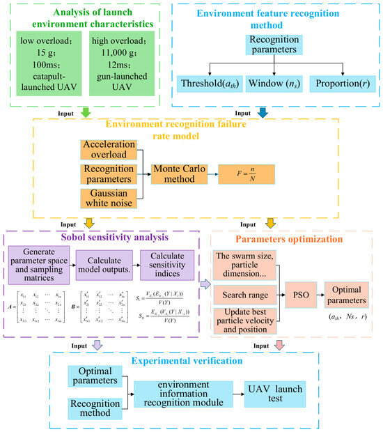
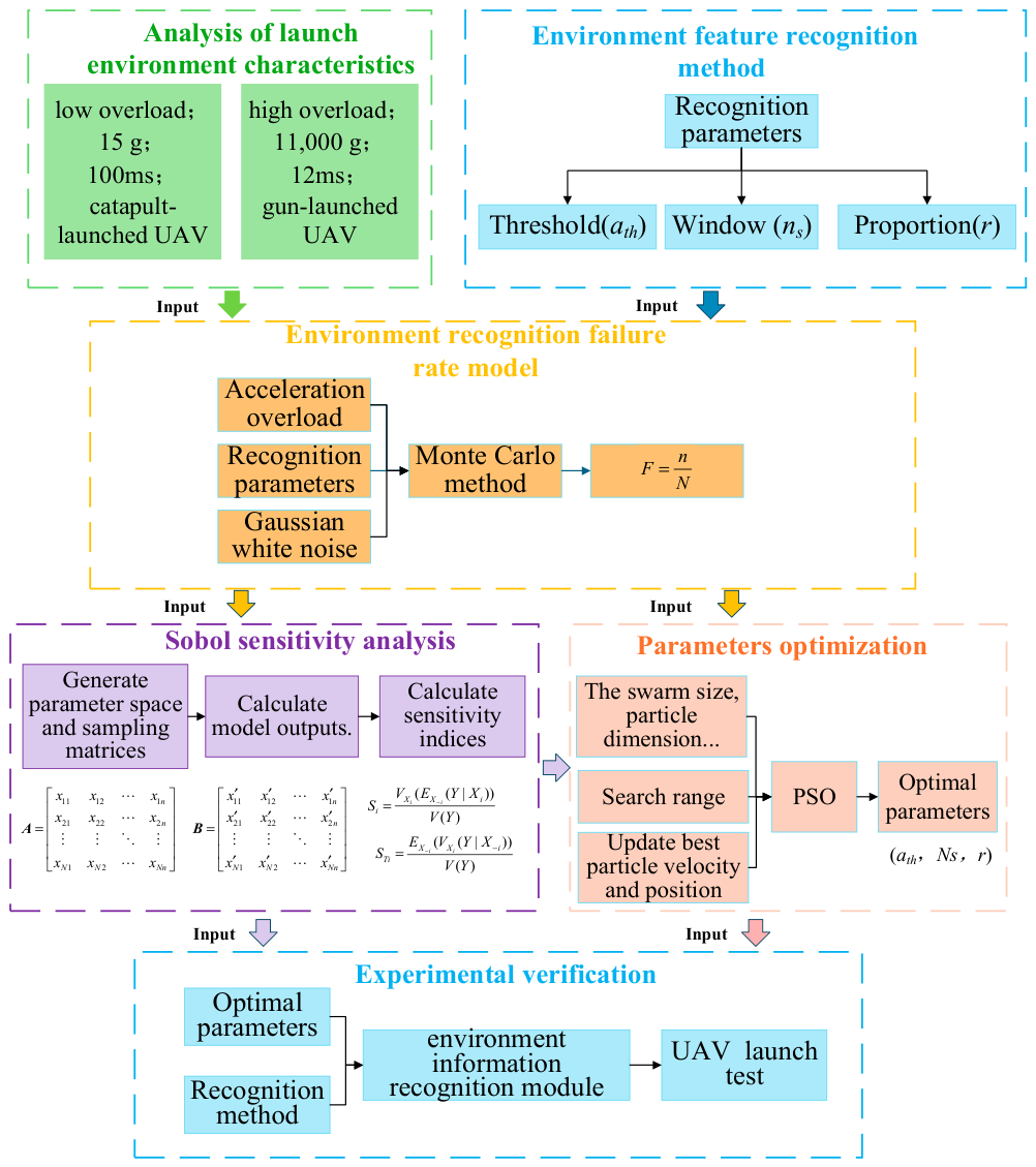
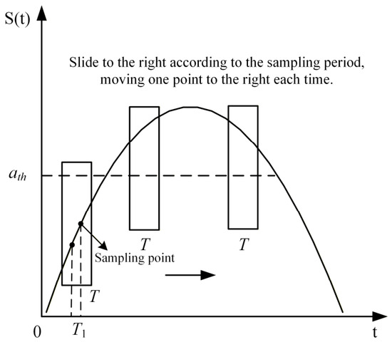
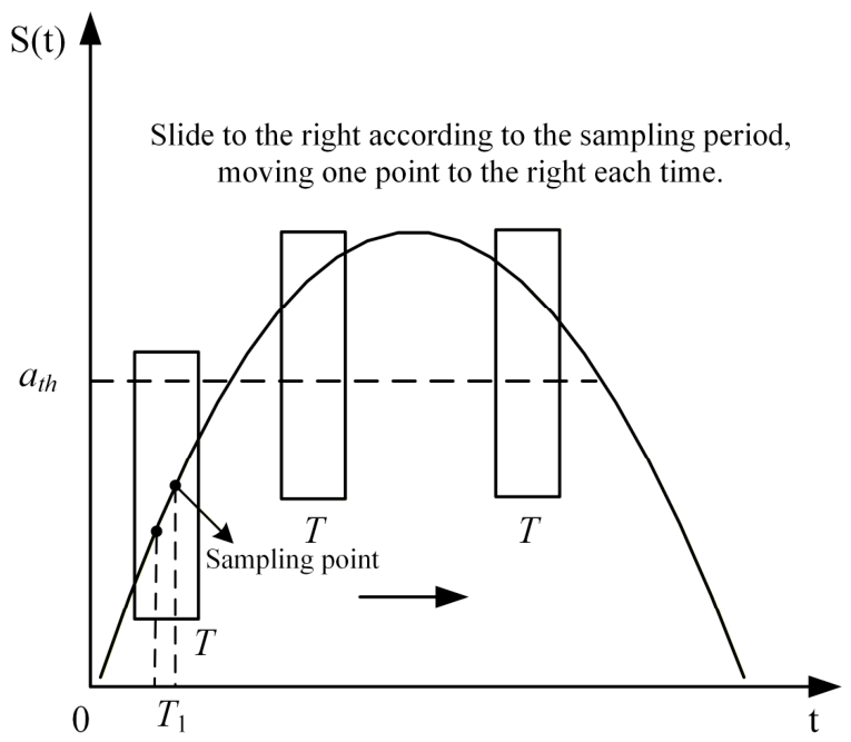
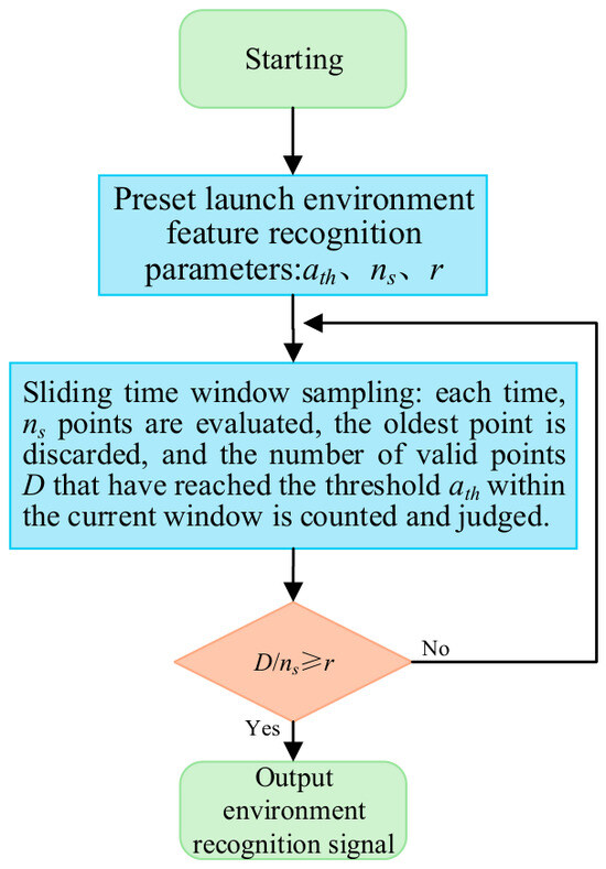
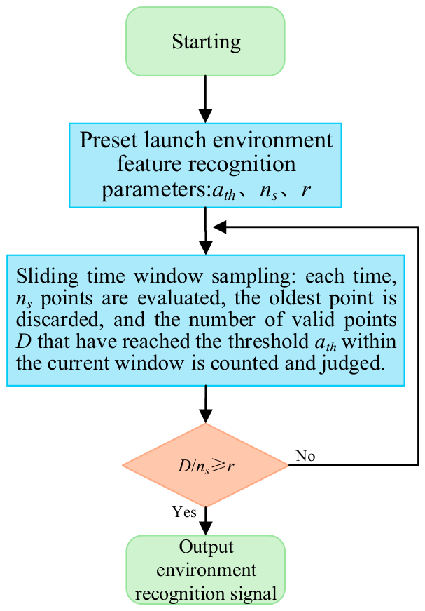
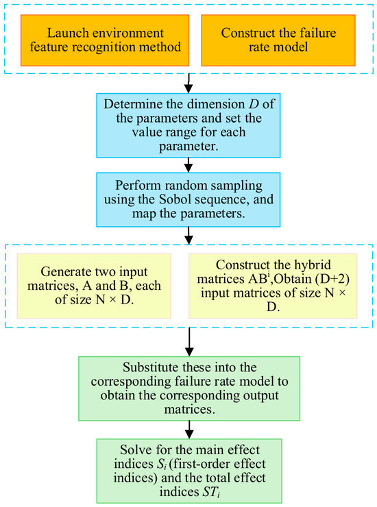
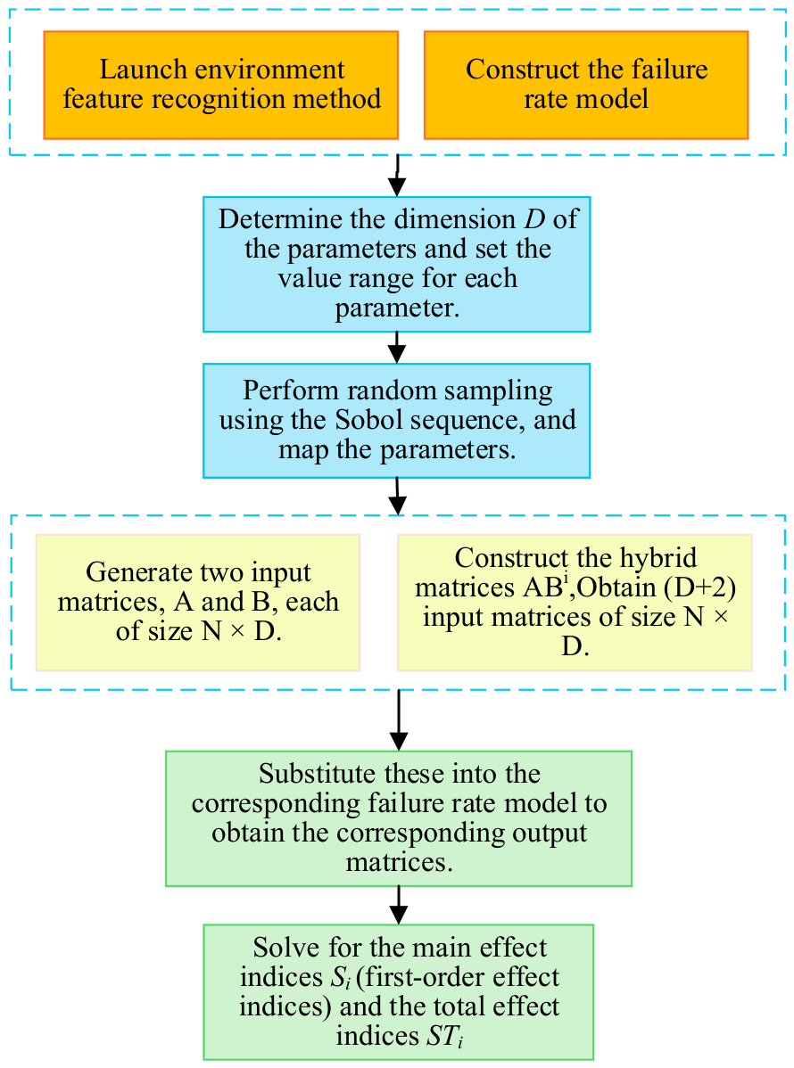
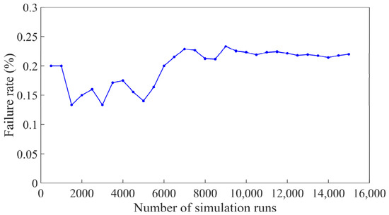
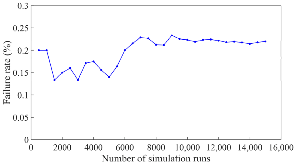
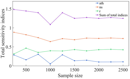
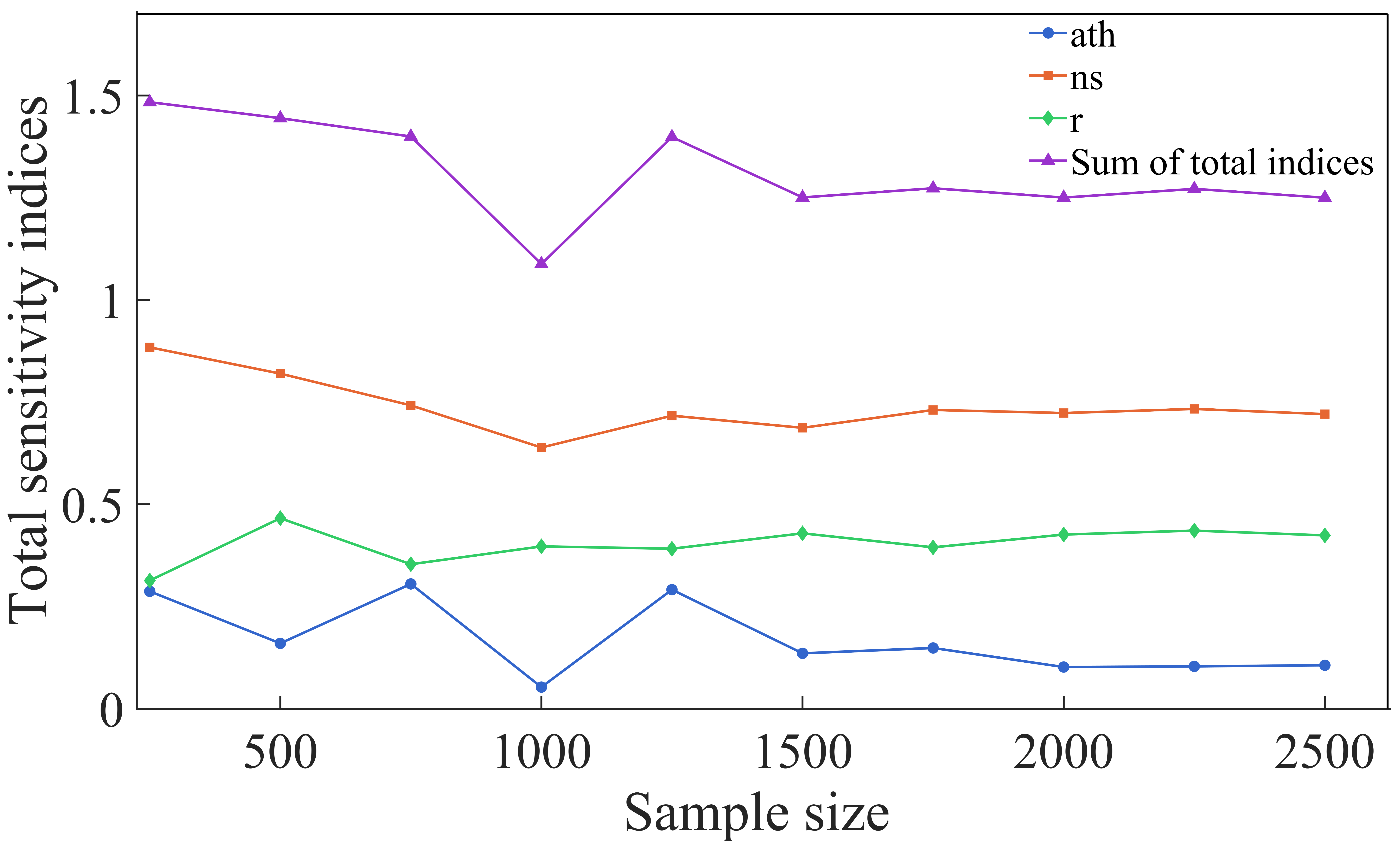
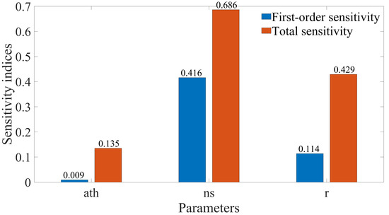
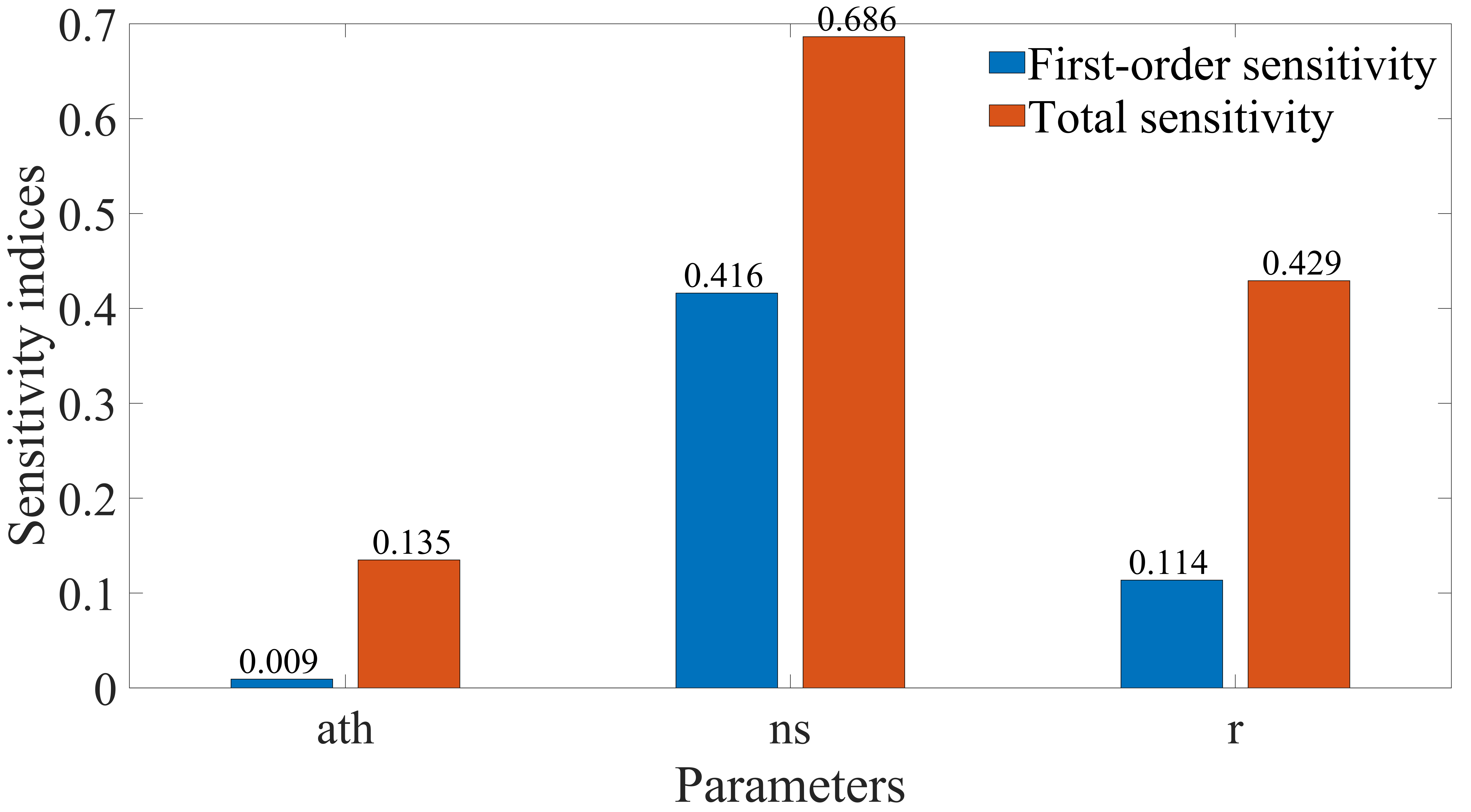
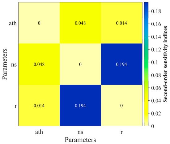
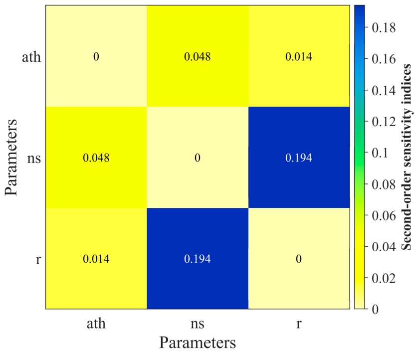
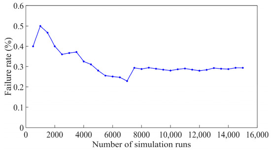
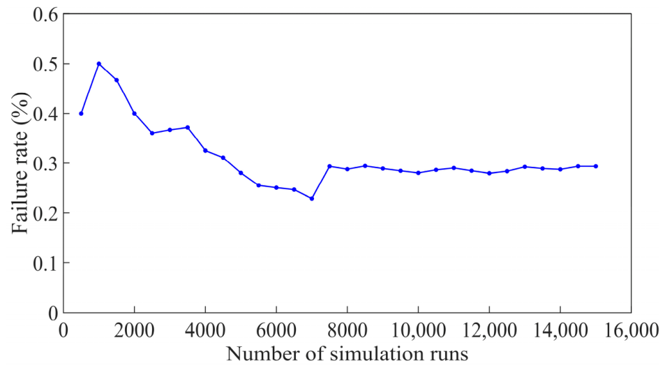
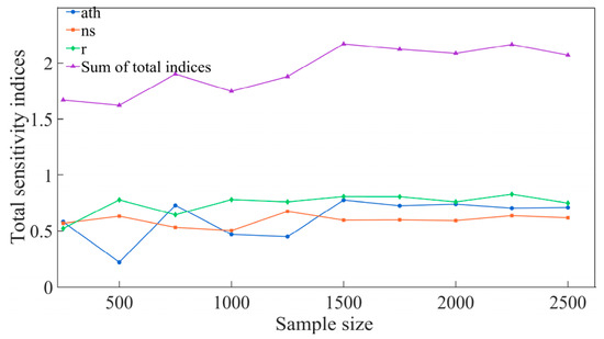
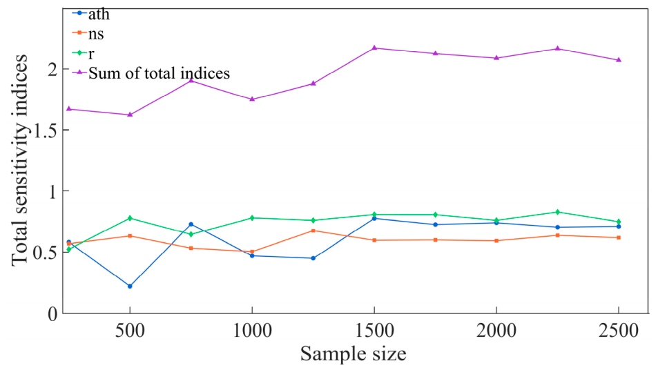
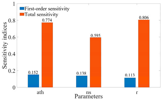
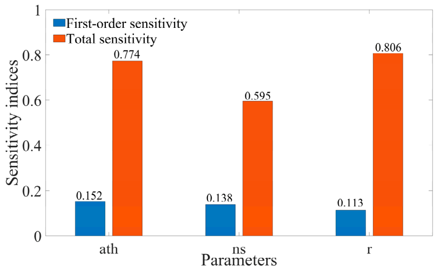
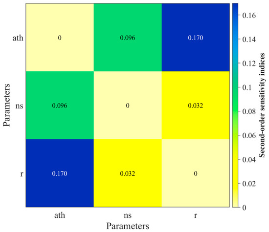
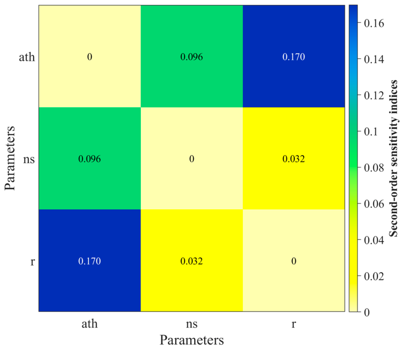
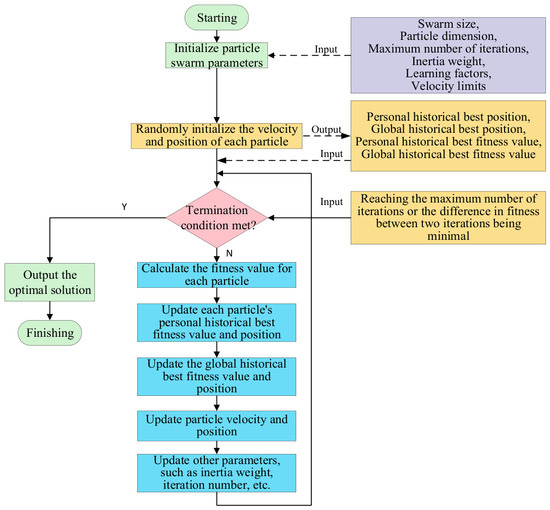
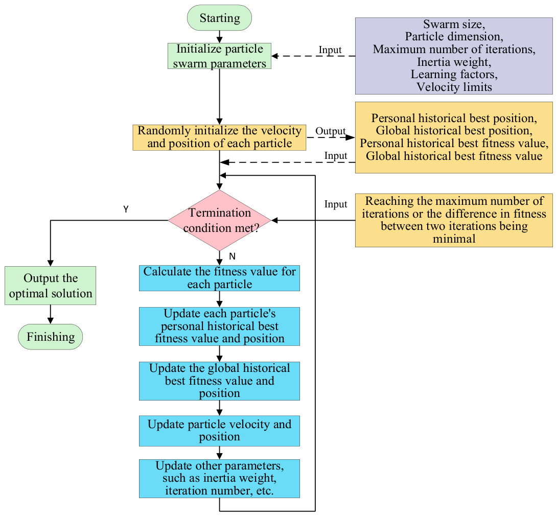
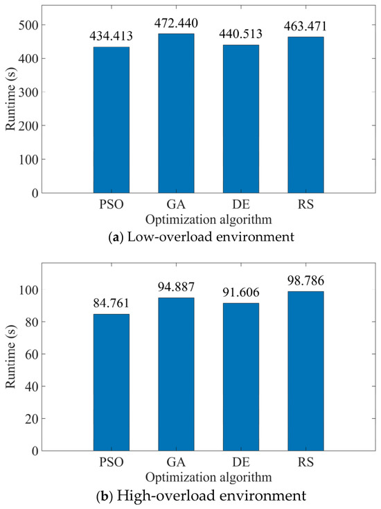
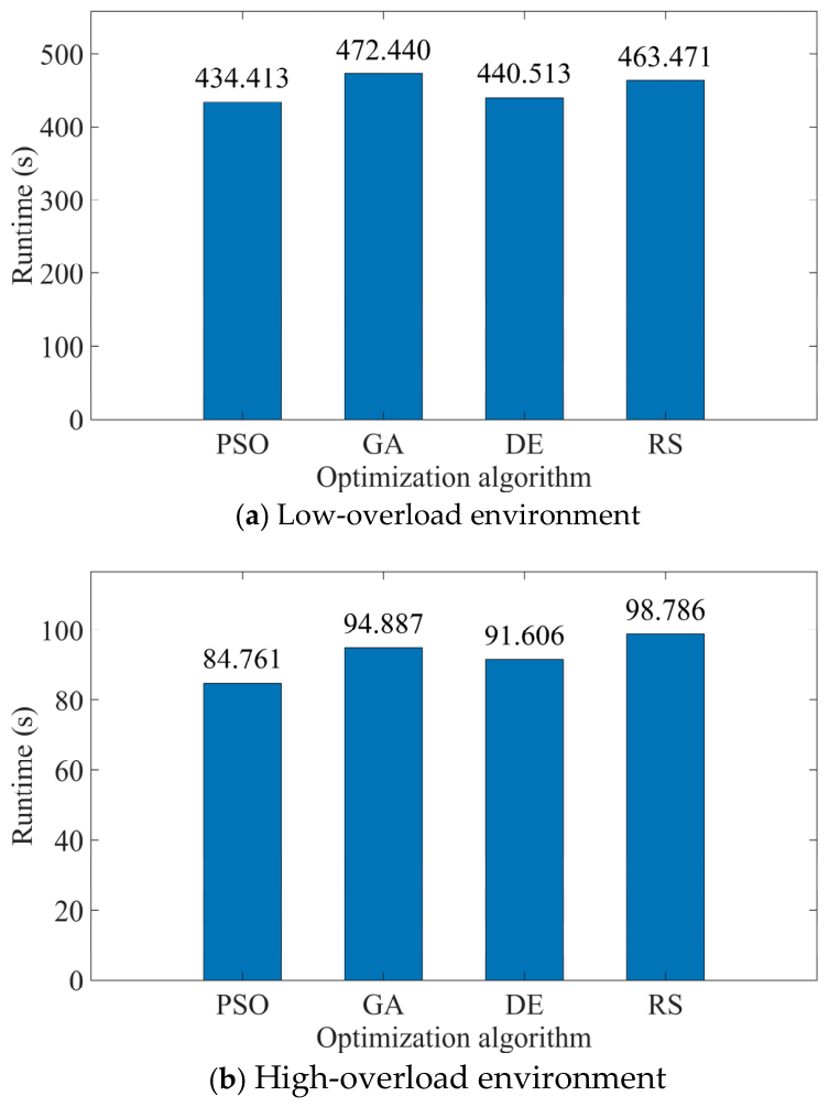
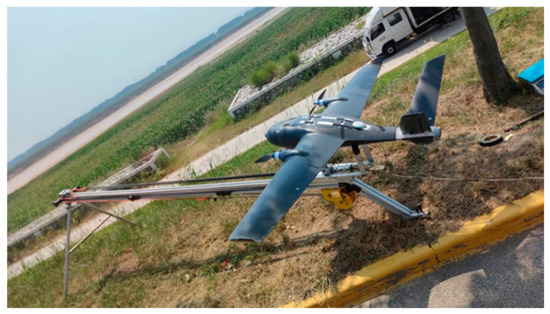
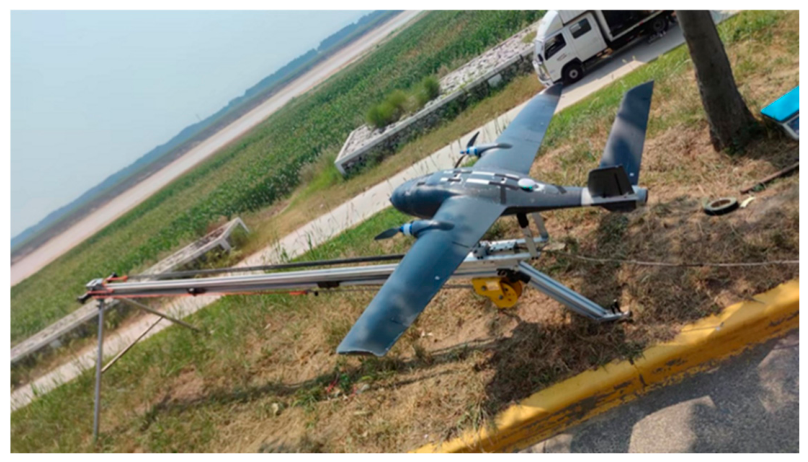
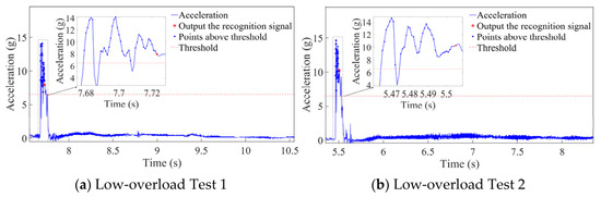
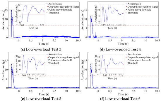
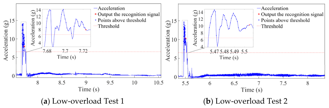
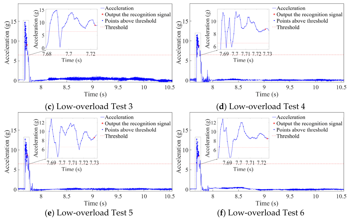
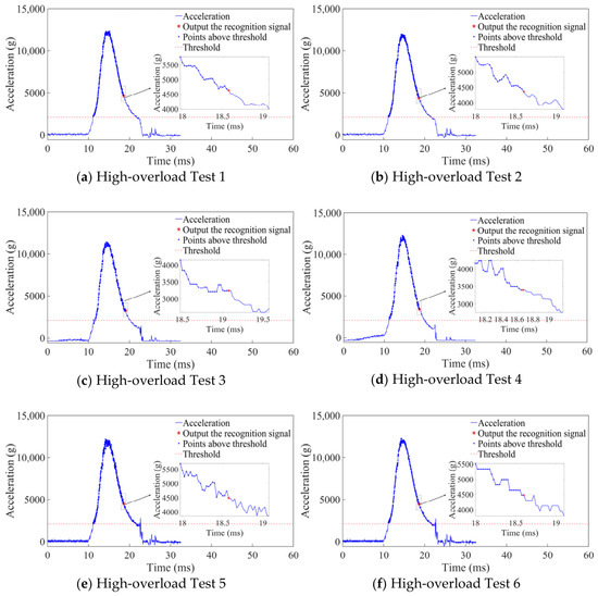
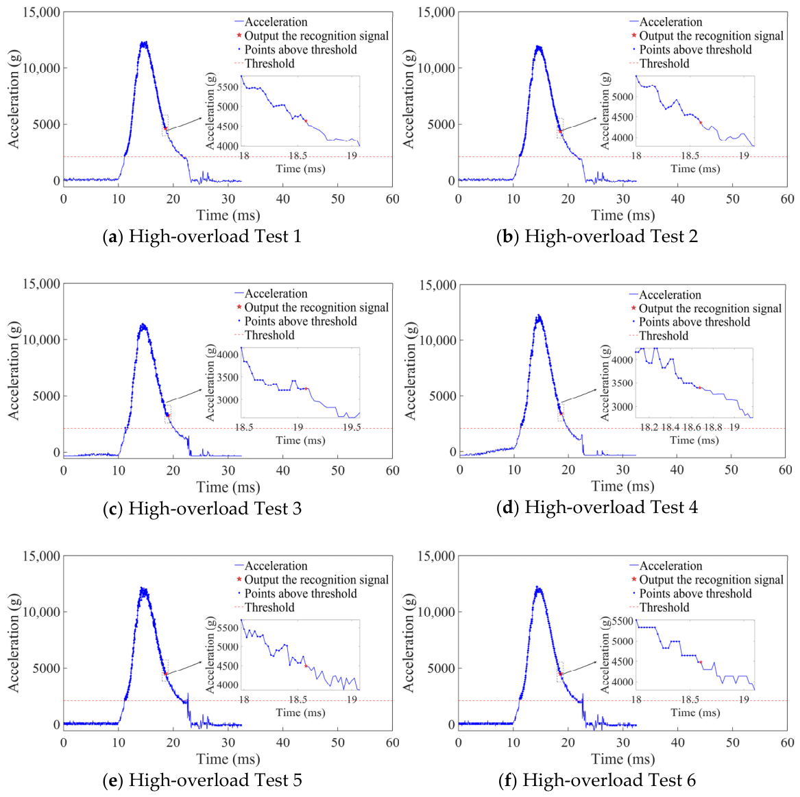
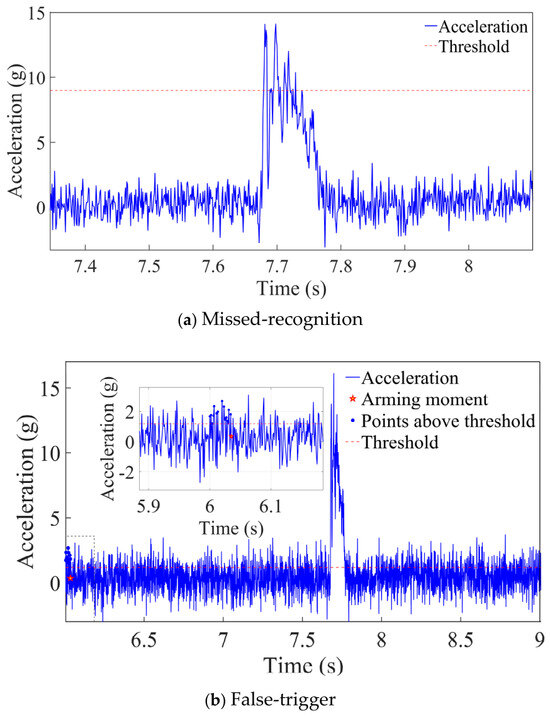
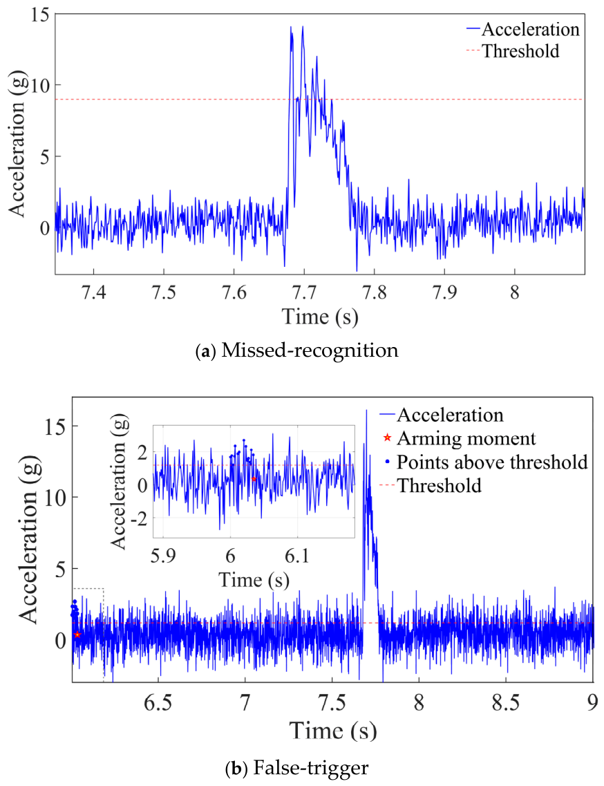

Disclaimer/Publisher’s Note: The statements, opinions and data contained in all publications are solely those of the individual author(s) and contributor(s) and not of MDPI and/or the editor(s). MDPI and/or the editor(s) disclaim responsibility for any injury to people or property resulting from any ideas, methods, instructions or products referred to in the content. |
© 2026 by the authors. Licensee MDPI, Basel, Switzerland. This article is an open access article distributed under the terms and conditions of the Creative Commons Attribution (CC BY) license.