


Abstract
Aircraft control surface systems are prone to resonance when the modal frequency of the transmission chain approaches the excitation frequency under varying load and operating conditions. To address this problem, this paper introduces a PEA-based preload regulation branch into the load bearing path of the transmission chain and develops a schedulable cross-layer mapping model from input voltage to modal frequency. The model follows the path of voltage, additional preload, axial equivalent stiffness, output side equivalent torsional stiffness, and modal frequency, and is used to judge whether the PEA branch has enough frequency shifting authority at a given working point. Based on this map, a resonance margin-constrained active stiffness scheduling method is established. Instead of applying a fixed or maximum voltage, the method calculates the minimum input voltage required to move the target modal frequency outside the dangerous resonance region. The numerical results show that increasing the voltage from 0 V to 150 V shifts the target modal frequency from approximately 56.4 Hz to 66.3 Hz, which indicates the available frequency regulation range of the added branch. For the studied excitation condition, the scheduler selects 64 V as the first feasible input and achieves a resonance margin of 1.003. The corresponding target mode RMS response is reduced by about 58.6%. Although the maximum voltage case gives stronger RMS attenuation, it requires larger preload and higher relative electrical energy demand. The proposed method is therefore not intended to maximize vibration attenuation under all conditions. It provides a resonance margin-based voltage selection rule that converts local PEA-based stiffness regulation into a system-level target modal frequency-scheduling mechanism for the studied transmission chain.
1. Introduction
Aircraft resonance avoidance is usually considered during the structural and flight control system design stage by separating the characteristic frequencies of the airframe, the control surface, and the actuation transmission chain. However, this frequency separation is not fixed during service. The modal frequencies of the airframe may vary because of fuel consumption, lightweight structural design, changing aerodynamic and inertial loads, payload variation, and long-term structural degradation. At the same time, the modal frequencies of the control surface transmission chain may also drift due to changes in assembly preload, contact stiffness, clearance, friction, load state, and the wear of mechanical interfaces. When the modal frequency of the transmission chain approaches excitation or a nearby airframe-related frequency, the originally designed resonance margin may be reduced, and the risk of vibration amplification in the control surface system increases [1,2].
Although the vibration of the control surface transmission chain alone is not necessarily a catastrophic problem, its frequency drift is relevant to aircraft safety because the control surface is directly involved in load transmission and attitude control. Once the frequency separation between the aircraft structure and the actuation system becomes insufficient, local transmission chain vibration may amplify output shaft angular fluctuation, increase dynamic load in the support and contact interfaces, and degrade the dynamic margin of the control surface system. Therefore, it is necessary to quantitatively analyze how nonlinear factors in the transmission chain affect the system modal frequency. Such analysis can support active parameter design at the structural level, and can also provide a basis for in-service resonance avoidance by adjusting key stiffness-related parameters when the aircraft operates under varying conditions.
Existing resonance- and vibration-suppression studies for actuation and flexible aerospace systems have mainly followed the route of feedback compensation, active damping, or control loop shaping. Li et al. proposed an adaptive disturbance-suppression method for servo systems based on a state equalizer to reduce the effect of high-frequency resonance disturbance [3]. Shui et al. developed a dual-loop electric servo loading strategy based on an H-infinity control framework for high-dynamic loading systems [4]. For flexible aerospace structures, Verhaegen and Żbikowski developed an aeroservoelastic model of a slender missile and designed active damping control, while Bülbül et al. integrated closed-loop control action into a transient finite element solution for active vibration control [5,6]. These studies show that feedback-based methods can suppress vibration response or improve closed-loop behavior near critical frequency bands. However, they usually regulate the control input after the structural dynamics have already been formed, and the transmission chain stiffness is commonly treated as a fixed, identified, or passively varying parameter.
Alternative research efforts have concentrated on structural optimization, damping enhancement, and adaptive vibration absorption. Preumont explained active damping and vibration isolation via the aspects of energy transmission and feedback control mechanisms [7]. Belyaev et al. compared local active control and modal active control for elastic systems [8]. Herold et al. studied an adaptive piezoelectric absorber, in which the resonant frequency can be adjusted according to different excitation conditions [9]. Peukert et al. and Zhang et al. also investigated local or modal vibration control methods and nonlinear vibration control in piezoelectric structures [10,11]. At the same time, several studies on piezoelectric actuator modeling and compensation have considered nonlinear input and output characteristics, such as hysteresis, tracking error, and Bouc–Wen-type nonlinear dynamics [12,13,14]. These works show that vibration performance can be improved by changing structural parameters or actuator-related parameters, when the tuning objective has been clearly given. However, most existing studies still do not directly explain how the local preload regulation inside a flight control transmission chain can be connected with the required separation of modal frequency.
Piezoelectric smart structure techniques offer a possible approach to local actuation, because piezoelectric actuators are able to produce displacement or force with high bandwidth in a compact component. Zhou et al. reviewed the recent progress of piezoelectric actuators in terms of materials, classifications, and engineering applications [15], while Marakakis et al. summarized shunt piezoelectric systems used for noise and vibration control [16]. For flexible structures, Biglar et al. optimized the locations of piezoelectric sensors and actuators for the active vibration control of plates [17]. Zhang et al. investigated the robust active vibration control of piezoelectric flexible structures under uncertainties [18], and Tsujiuchi et al. presented modal vibration control by using piezoelectric films [19]. These studies show that piezoelectric elements can interact with structural modes in a feasible way. However, for a flight control transmission chain, this feasibility cannot be explained only by the actuation ability of piezoelectric elements. The added actuation branch should also be considered together with the limitations of mass, volume, power consumption, preload, and structural integration.
In aerospace applications, adaptive vibration suppression and aeroelastic control have also been studied for wings, morphing structures, and spacecraft systems. Ahmed and Mahmood adopted acceleration feedback to reduce the vibration of an acrobatic aircraft wing [20], and O’Donnell et al. investigated the active aeroelastic control of a wing model through synthetic jet actuation [21]. Ajaj et al. reviewed recent progress in the aeroelasticity of morphing aircraft [22]. Xu et al. analyzed an active variable stiffness vibration isolator for spacecraft systems [23], while Sheng et al. studied the aeroelastic vibration reduction of a supersonic cantilever wing plate based on nonlinear metamaterials [24]. These studies indicate that adaptive structural dynamics are highly relevant to aerospace systems. However, they still do not give a direct design rule for how to schedule the stiffness of a compact control surface transmission chain. Moreover, a complete aeroelastic suppression problem usually contains the coupling among aerodynamic loads, structural dynamics, and control loops. Therefore, the present work is restricted to the mechanical resonance margin problem of the transmission chain, which may be regarded as one part of the broader aeroservoelastic design problem.
Considering the above issues, the main question of this paper can be stated as follows: under a given operating condition and a dangerous excitation frequency, whether a local preload input generated by PEAs can provide enough modal frequency separation for the control surface transmission chain, and whether the required voltage can be chosen without using unnecessary high voltage operation. To deal with this question, an active stiffness regulation branch using PEAs is introduced into the load-bearing path of the transmission chain. Then, a forward cross-layer model is established along the path from input voltage, additional preload, axial equivalent stiffness and output side equivalent torsional stiffness, to modal frequency. Based on this model, the resonance avoidance problem is transformed into a minimum voltage scheduling problem constrained by the required resonance margin. The numerical study further examines the available frequency regulation range, the resonance margin recovery, the target mode response after scheduling, and the feasibility boundary of the proposed method.
The main contributions of this paper are as follows. First, a PEA-based preload regulation branch is introduced into the load-bearing path of an aircraft control surface transmission chain. This branch provides a structural parameter scheduling channel while keeping the main displacement transmission path and the primary flight control actuator unchanged. Second, a voltage to frequency map is established through additional preload, axial equivalent stiffness, output side equivalent torsional stiffness, and modal frequency. The purpose of this map is not only to describe the stiffness transmission path, but also to quantify whether the local preload regulation has sufficient modal frequency authority at a given working point. Third, a resonance margin-constrained minimum voltage scheduling method is formulated. Different from empirical fixed voltage regulation and maximum detuning regulation, the scheduled voltage is selected from the required modal separation and the admissible actuator range. Numerical simulations are then used to examine the mapping relation, the scheduling feasibility, the target mode response, and the implementation demand of the PEA branch.
2. PEA-Based Active Stiffness Regulation System
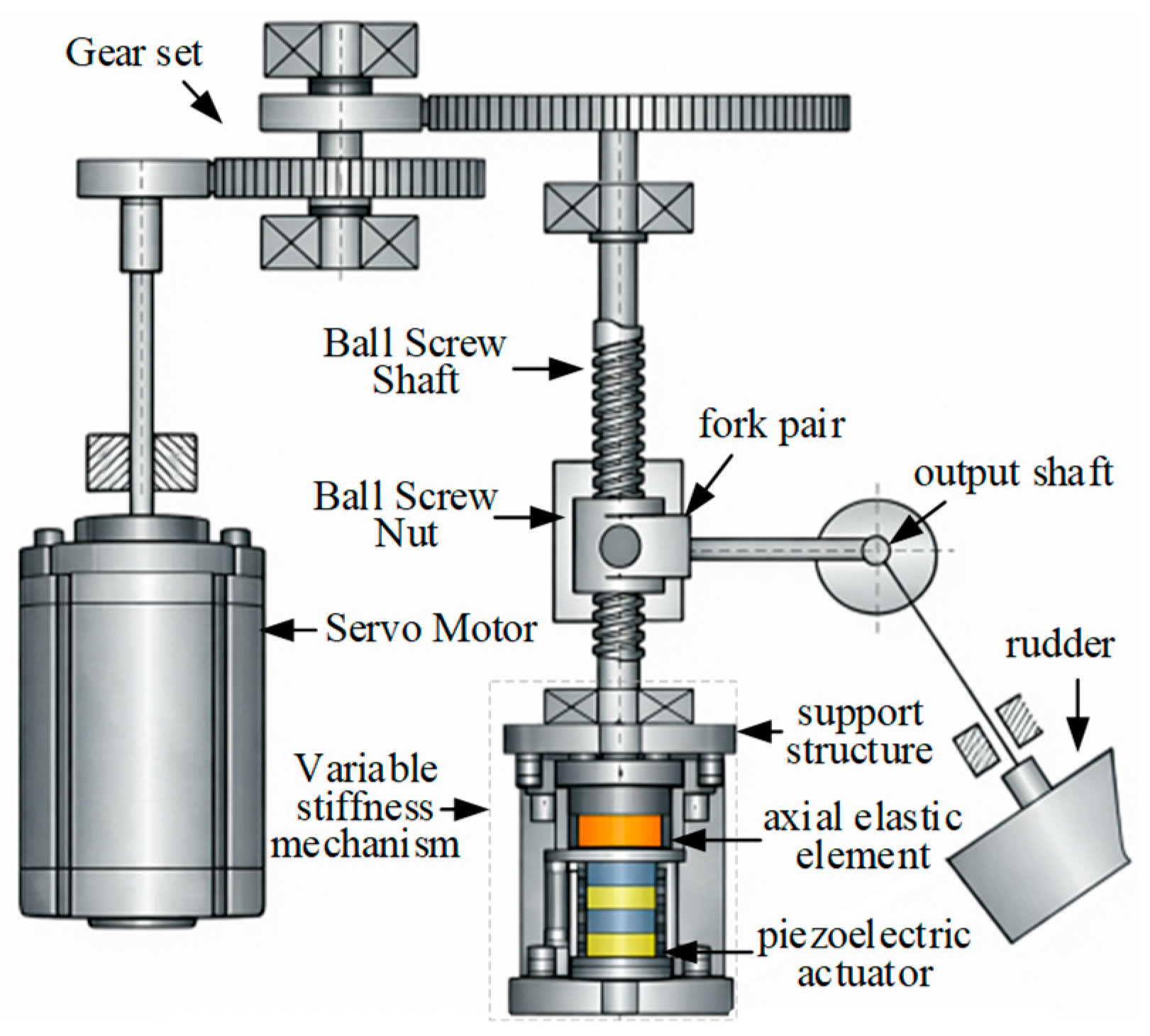
The active stiffness regulation system considered in this paper is constructed by adding an auxiliary PEA-based preload regulation branch to the load-bearing path of a conventional control surface transmission chain. This branch is not used as the primary flight-control actuator and does not directly command the control surface deflection. The original actuator still provides the motor torque and the prescribed output shaft motion through the gear set, ball screw, fork pair, and output shaft. The function of the added branch is limited to modifying the axial preload state of the ball screw support path, thereby changing the local support and contact stiffness and the equivalent stiffness projected to the output side. In this sense, the proposed system introduces a structural parameter scheduling channel while keeping the main displacement transmission path unchanged.
2.1. Stiffness Regulation Branch
The baseline transmission chain consists of the servo motor, gear set, ball screw shaft, ball screw nut, fork pair, output shaft, and control surface. In the baseline configuration, the commanded rotation of the motor is transmitted to the control surface through the displacement path of motor rotation, gear reduction, screw rotation, nut axial translation, fork swing, and output shaft rotation. In the proposed configuration, a PEA-based stiffness regulation branch is installed along the axial support path of the ball screw. The branch consists of a PEA stack, an axial elastic element, and a support structure. After a voltage command is applied, the small actuator stroke is converted into an additional axial preload through the elastic element and installation path. This preload modifies the local tangent stiffness of the support and contact path, but it does not introduce an additional commanded displacement into the control surface output coordinate. The overall configuration of the control surface system with the added PEA-based stiffness-regulation branch is shown in Figure 1.
Figure 1.
Stiffness active adjustment control surface system overall configuration.
2.2. Displacement Transmission and Load Transfer Paths
The displacement transfer path of the baseline control surface system follows the sequence of motor rotation, gear reduction, ball screw rotation, nut axial displacement, fork swing, and output shaft rotation. The load transfer path works in the opposite direction. The aerodynamic and control surface loads are transmitted from the control surface through the output shaft, fork, nut, ball screw, and end support to the actuator housing, as illustrated in Figure 2. The actuator is placed within this load-bearing path, so that a small actuator stroke can adjust the support preload and contact stiffness without directly commanding any control surface displacement.
Figure 2.
Displacement and force transfer path.
The present model focuses on the modal frequency scheduling effect caused by preload-induced stiffness variation. Therefore, the added PEA branch is simplified as a voltage-controlled preload source connected to the axial support path through an equivalent elastic element. The detailed internal dynamics of the high-voltage driver, local installation compliance, and actuator hysteresis are not modeled as independent dynamic states in this section. Their combined influence is included later through the effective displacement relation and the residual term in the voltage-to-preload mapping. This modeling choice is suitable for evaluating whether the added branch has sufficient frequency-shifting authority near a given operating point. It is not intended to describe large-range contact switching impact response, or full aeroservoelastic coupling.
3. Cross-Layer Mapping Model
The derivation in this section is arranged for stiffness scheduling. It is not intended to rederive a complete stiffness theory for the screw and fork transmission. The purpose is to obtain a usable forward map from the PEA voltage to the target modal frequency, so that the available stiffness regulation authority can be judged before the voltage is scheduled.
3.1. Voltage to Preload Mapping
Let denote the input voltage of the PEA branch, the effective axial displacement of the PEA stack under the installation constraint, and the additional preload generated by the PEA branch. The total axial load acting on the ball-screw support path is denoted by . The forward cross-layer action chain from voltage input to modal frequency variation can then be expressed as
The cross-layer action chain of the active stiffness-regulation control surface system is illustrated in Figure 3. This chain provides the forward map used by the scheduler. Through this map, the modal frequency reachable by local stiffness regulation can be estimated for a given working point and voltage input.
Figure 3.
Forward cross-layer map used for stiffness scheduling.
The constrained PEA output is not an ideal linear displacement because hysteresis, rate dependence, and local assembly disturbance may exist [25]. Therefore, the effective input near the working point is uniformly expressed as
where is the effective actuation displacement of the actuator under the current constraint boundary, is the initial preload, characterizes the effect of input frequency or input interval, and is the deviation term caused by hysteresis, rate dependence, and local installation disturbance [26,27].
The effective actuator displacement is converted into additional preload through the axial elastic element and the installation path. Denoting the equivalent installation transfer coefficient as , the preload increment near the working point can be approximately written as
where is the stiffness of the axial elastic element in the stiffness adjustment mechanism. Substituting Equation (2) into Equation (3), we can get
Near the working point, the axial total load of the ball screw pair and the end support path can be expressed as
To define the applicable range of the cross-layer mapping, the following assumptions are made.
- (a)
- The mapping is built near the static equilibrium point determined by the given initial preload, control surface angle, and external load. The stiffness and modal frequency changes caused by the PEAs are treated as small local perturbations around this working point.
- (b)
- Within the studied regulation range, the contact topology of the ball screw, bearing, and support interfaces is assumed to remain unchanged. Contact loss, contact establishment, and impact events are not considered. The preload-dependent contact stiffness is treated as the tangent stiffness at the current working point.
- (c)
- The relationship between nut axial displacement and output shaft rotation is locally linearized within a small angle range. The geometric mapping coefficient is considered constant only at a fixed working point. When the control surface angle or load state changes beyond the selected local range, the coefficient should be updated together with the current working point.
- (d)
- The active branch is assumed to mainly affect the local equivalent stiffness and its contribution to the system stiffness matrix. The mass matrix is kept unchanged in the local model, and damping variation together with higher-order coupling effects are absorbed into residual terms.
3.2. Preload to Axial Stiffness Mapping
The axial equivalent stiffness of the ball screw support path is determined by several stiffness components connected in series and parallel, including the ball nut contact stiffness , the axial stiffness of the screw shaft , and the support structure stiffness , as shown in Figure 4. The two end supports are treated as symmetric load-bearing paths. For each side, the elastic element stiffness and the bearing support stiffness are connected in series, and the two sides are then combined as parallel branches.
Figure 4.
Axial equivalent stiffness composition.
Based on the Hertz contact theory [28], the bearing support stiffness can be expressed as
where represents the comprehensive coefficient related to material, contact geometry, ball distribution and local boundary.
For the following voltage to frequency map, the equivalent stiffness of the noncontact part is written as
The axial equivalent stiffness can be written as
3.3. Axial to Torsional Stiffness Mapping
Near a fixed working point, the small axial displacement of the ball screw nut and the small rotation angle of the output shaft are related by
where is the small axial displacement of the nut and is the small rotation angle of the output shaft. is the local geometric mapping coefficient at the current working point, which describes how efficiently a local axial stiffness variation is projected onto the output-side rotational coordinate. This coefficient is a local quantity. It varies with the control surface angle and load state, and it should not be used as a global constant.
Based on the principle of virtual work, the equivalent torsional stiffness of the output side can be obtained as
When is small, the torsional stiffness increment corresponding to the axial equivalent stiffness change on the output side is small; when is large, the effect of axial equivalent stiffness change on the equivalent torsional stiffness of the output side is more significant.
Combined with the above derivation, the relationship between the equivalent torsional stiffness of the output side and the actuator input can be expressed as
Equation (11) shows that the actuator input is not transmitted to the output-side stiffness through a simple proportional relationship. Instead, the achievable stiffness increment is jointly constrained by the PEA actuation capability, the preload-dependent contact stiffness, the series stiffness of the support path, and the geometric transmission efficiency.
The first-order linearization near the current working point can be obtained
The local stiffness authority of the PEA branch is determined by the geometric mapping coefficient, the load sensitivity of the contact stiffness, the series stiffness of the support path, and the voltage-to-preload gain of the actuator branch. Therefore, even if the PEA voltage is increased, the output-side stiffness increment may still be limited by the decreasing load sensitivity of the contact stiffness, weak geometric projection, or low modal participation.
3.4. Torsional Stiffness to Modal Frequency Mapping
The output-side equivalent torsional stiffness increment is introduced into the system stiffness matrix near the working point, which gives a voltage-dependent modal frequency map. This map serves as the model basis for active stiffness scheduling.
The generalized eigenvalue problem of the system near the working point can be written as
where is the stiffness matrix of the system, is the mass matrix, and and are the order modal frequency and modal vector, respectively.
Within the local regulation interval considered in this study, the active stiffness branch mainly perturbs the stiffness matrix. The system stiffness matrix can therefore be written as
where represents the basic stiffness matrix without stiffness adjustment increment. The vector is the stiffness assembly vector of the output side equivalent torsional stiffness. Since is projected to the output shaft rotational coordinate in this study, it is taken as .
From the first-order eigenvalue relationship, it can be determined that
According to Equation (14), we can get
The sensitivity coefficient of the order mode to the output-side equivalent torsional stiffness is defined as
Equation (16) can be rewritten as
Equation (18) gives the local frequency gain used by the scheduler. It shows that the voltage input can shift the target modal frequency only when two conditions are satisfied. The PEA branch should generate a sufficient output-side stiffness increment, and the target mode should have enough sensitivity to this stiffness component. The fully expanded derivative is not listed separately, because it only follows the chain rule of the voltage-to-stiffness map. Equation (18) is sufficient for the scheduler to evaluate the local frequency gain once the voltage-dependent stiffness matrix has been updated.
The above voltage to frequency map is a local map. It is constructed around the working point, which is determined by the initial preload, the control surface angle, and the external load. The geometric coefficient should be understood as a local tangent coefficient, .
Therefore, , , , and should be updated when the working point changes. In the numerical scheduling procedure, the map is kept fixed only inside the selected local range. If the variation of the control surface angle, external load, or preload exceeds this range, the current map is recalculated before the voltage is selected.
4. Resonance Margin Constrained Active Stiffness Scheduling
4.1. Definition of Resonance Margin
For resonance avoidance, the key decision is not only to predict , but also to determine whether the target modal frequency is sufficiently separated from the dominant excitation frequency. In this study, the resonance risk is described by the normalized separation between the target modal frequency and the dangerous excitation frequency. Let denote the dangerous excitation frequency. A frequency separation expressed only in hertz is not sufficient to judge resonance avoidance, because the effective dangerous interval is related to the resonance bandwidth of the target mode. Therefore, a reference bandwidth is introduced to normalize the frequency separation [29]. The normalized resonance margin is defined as
where can be used when the damping ratio of the target mode is available. denotes the equivalent damping ratio of the target mode after stiffness regulation.
In the present numerical case, the PEA branch shifts the target modal frequency to the high-frequency side, and the damping variation caused by preload change is not calibrated by test data. Therefore, the baseline calculation uses the zero-input reference bandwidth . This treatment does not imply that the actual damping remains unchanged during preload regulation. It only provides a fixed reference bandwidth for the baseline scheduling case when preload-dependent damping data are not available. Under this condition, Equation (19) is reduced to
If the resonance peak is clearly asymmetric, the bandwidth in Equation (20) can be replaced by the corresponding side’s bandwidth on the side closer to . In the following numerical study, this asymmetric bandwidth is not introduced because the response model is used only for a baseline scheduling assessment.
When , the target modal frequency is still close to the dangerous excitation frequency within one reference bandwidth, and the resonance avoidance effect is limited. When , the active stiffness branch has just recovered the basic frequency separation defined by the selected bandwidth. When , the target modal frequency has been moved outside the main reference bandwidth. In this paper, the required safety level is represented by a prescribed safety coefficient , so the resonance margin requirement is written as
The margin in Equation (21) is defined for the selected target mode. It does not replace the check of adjacent modes. When closely spaced modes exist, the same separation check should be applied to the neighboring modes in the dangerous frequency band.
This requirement changes the purpose of active stiffness regulation from simply increasing the modal frequency to maintaining a quantifiable frequency separation. A small frequency increase may be physically observable, but it is still not enough for resonance avoidance if the normalized margin is lower than the prescribed value.
4.2. Minimum Voltage Scheduling Formulation
Given a prescribed safety coefficient γ, the scheduling problem is first considered in a minimum feasible input form. In this form, the scheduled voltage is selected as the smallest voltage that satisfies within the admissible voltage range. This formulation avoids unnecessarily high voltage and excessive preload when a smaller voltage is already sufficient for resonance margin recovery.
The cross-layer map in Section 3 provides the forward map from voltage to modal frequency, which can be written as
where denotes the voltage to frequency map at the current working point; , , and denote the generalized working state, initial preload, and control surface angle, respectively. The map is obtained through the chain . The scheduling problem is formulated as
subject to
The above formulation contains two parts. The first part is the resonance margin constraint, which determines whether the target mode is sufficiently separated from the dangerous excitation frequency. The second part is the physical admissibility constraint of the stiffness regulation branch, including voltage limit, preload limit, and unchanged contact state.
In a practical implementation, the scheduled voltage may also be evaluated by actuator-related cost. A more general engineering cost can be written as
where , , , and are non-negative weighting coefficients. The four terms describe voltage usage, preload usage, relative electrical energy, and hysteresis-related uncertainty, respectively. is an index used to represent the uncertainty caused by the voltage increasing and decreasing paths or the local hysteresis loop width.
In the present numerical case, these weighting coefficients are not calibrated by experimental lifetime or reliability data. The main purpose is to identify the first feasible voltage satisfying the resonance margin constraint. Therefore, the general cost in Equation (25) is reduced to the minimum voltage form,
Therefore, the solution is the smallest voltage that satisfies the resonance-margin requirement and the physical constraints of the stiffness-regulation branch.
The reduced objective in the above equation is consistent with the practical intention of avoiding unnecessary voltage when the required resonance margin has already been reached. Excessive voltage may increase preload demand, driver stress, hysteresis uncertainty, and energy consumption. When the frequency map is monotonic over the studied voltage interval, the reduced problem can be solved by a one-dimensional search. When local non monotonicity appears due to hysteresis or operating condition dependence, the admissible voltage grid can be scanned and the first feasible voltage is selected.
For a monotonic high-frequency shift, the scheduling law can also be interpreted as an inverse map. The required target frequency is
The required voltage is then the smallest voltage satisfying . This inverse interpretation clarifies why the proposed method differs from an open-loop voltage sweep. The voltage is determined from a resonance avoidance target rather than being prescribed arbitrarily.
To indicate how uncertainty can be included, the resonance margin constraint can also be written in a conservative form. Let denote the uncertainty in excitation frequency, reference bandwidth, voltage to preload gain, and hysteresis deviation. The robust feasibility condition is
or equivalently,
In this paper, Equation (28) is not solved as a full robust optimization problem. Instead, the influence of excitation frequency, reference bandwidth, and voltage to preload mapping uncertainty is examined by sensitivity analysis in the numerical section.
4.3. Feasibility and Physical Conditions
The scheduling problem is feasible only when the required margin can be reached without violating the voltage, preload, contact state, and local mapping validity constraints. If , the active stiffness branch is considered insufficient for that operating condition. This infeasibility result is useful because it identifies the boundary beyond which passive stiffness redesign, damping enhancement, or excitation frequency avoidance becomes necessary. In addition, if the current working point moves outside the local range used to construct the voltage to frequency map, the scheduled voltage should not be applied directly before the map is updated.
The minimum voltage solution is physically meaningful only when it satisfies the constraints of the active stiffness branch. In addition to the voltage bound, the total preload must remain within the admissible contact range, as follows:
The constant contact state assumption requires that contact interfaces do not detach, experience impact, or switch topology during regulation. This condition is written as
Furthermore, the available frequency shift is limited by the maximum voltage and by the decreasing sensitivity of the preload-dependent stiffness relation. The maximum reachable resonance margin is defined as
The local voltage to frequency map is valid only inside a local working point domain. This domain is denoted as . A simple form can be written as
If , the current map should be updated before scheduling. In this case, , , , and the modal frequencies are recalculated according to the current rudder angle, preload state, and load state.
The feasibility flag is not only determined by the target mode. It also requires that no adjacent mode is shifted into the dangerous frequency band during stiffness regulation. Let denote the dangerous frequency band around . For the non-target modes in the considered frequency range, the following condition should be satisfied,
During implementation, this condition should be checked by monitoring the modal frequencies near the dangerous band when a calibrated multi-mode model or measured modal data are available.
The scheduling problem is feasible only when the following conditions are satisfied,
If the first condition is not satisfied, the active stiffness branch does not have sufficient modal frequency authority under the current working condition. If the preload or contact condition is violated, the scheduled voltage is not physically admissible. If , the result is not directly infeasible, but the local map must be updated before a decision is made. If a neighboring mode enters the dangerous frequency band, the current voltage is rejected even when the target mode satisfies the resonance margin requirement.
4.4. Scheduling Algorithm
The scheduling procedure works as follows. First, the local voltage to frequency map is checked and updated according to the current working point. Then, the zero input resonance margin is computed. If the zero-input condition already satisfies the required margin and the adjacent modes are outside the dangerous band, is set. Otherwise, the admissible voltage interval is searched and the first feasible voltage satisfying the target mode margin, physical constraints, and adjacent mode separation condition is selected. If the local map is no longer valid, the procedure reports that a mapping update is required. If no feasible voltage exists after the map update, the condition is reported as infeasible.
Input: current working point , excitation frequency , reference bandwidth , safety coefficient , voltage limits , preload and contact constraints, local validity thresholds and , and adjacent mode separation requirement.
- Step 1: Check whether the current working point belongs to . If it is outside this local domain, update , , , and the modal frequencies according to the current rudder angle, preload state, and load state. Then construct the cross-layer frequency map over the admissible voltage interval.
- Step 2: Compute the zero-voltage margin . If and the adjacent mode separation condition is also satisfied, set , because the system already has sufficient separation from the excitation band.
- Step 3: If , evaluate over the admissible voltage interval and identify the candidate set
- Step 4: If is non empty, choose . Then check the hysteresis-induced uncertainty and the voltage to preload mapping uncertainty if the uncertainty bounds are available. If the conservative margin is still satisfied, apply to the actuator branch.
- Step 5: If , report the condition as mapping update required. If is empty after the map has been updated, report the condition as infeasible under the current working point and output as the reachable resonance margin limit.
This procedure provides four outputs, as follows: the scheduled voltage , the achieved resonance margin , the feasibility flag, and the map validity flag. The advantage of this scheduling formulation is that it avoids treating the actuator voltage as a trial-and-error tuning parameter. The voltage is determined by a resonance margin requirement, while the local validity and adjacent mode constraints prevent the scheduler from using a local map outside its applicable range.
In practical use, the above procedure should be implemented with an offline calibrated map and an online working point update. The offline calibration gives the voltage to preload map, the local geometric coefficient, the reference bandwidth, and the admissible voltage and preload ranges. The online part updates the current working point, estimates or identifies the dangerous excitation frequency, and then searches the calibrated voltage to frequency map. If the working point is outside the calibrated local range, the scheduler should report map update required rather than directly applying the voltage command. If no feasible voltage exists after the map update, the system should keep the active stiffness branch within the admissible preload range and rely on other measures such as damping enhancement, excitation avoidance, or passive stiffness redesign.
5. Numerical Evaluation and Strategy Comparison
This section gives a representative numerical evaluation of the proposed scheduling method. First, the forward cross-layer map from PEA voltage to preload, stiffness, and target modal frequency is evaluated. Second, the resonance-margin-constrained scheduler is tested under a prescribed dangerous excitation frequency and different safety coefficients. Third, the sensitivity of the scheduled voltage to excitation frequency, reference bandwidth, and voltage-to-preload mapping uncertainty is examined. Fourth, an equivalent target mode response model is used to assess the response tendency of the selected target mode. Finally, the proposed minimum-voltage strategy is compared with empirical fixed-voltage regulation and maximum-detuning regulation in terms of resonance margin feasibility and implementation demand.
5.1. Parameter Sources and Numerical Case Assumptions
The parameters used in this section are listed in Table 1. They are used to construct a representative numerical case for examining the voltage to frequency map and the resonance margin constrained scheduling logic. Some parameters are obtained from the adopted transmission geometry or from the local stiffness model in Section 3. Some actuator and scheduling parameters are selected according to the admissible range assumed for the PEA branch. The remaining parameters are representative numerical values used to form a near-resonance condition.
Table 1.
Basic physical parameters and source of the representative numerical case.
These parameters are not intended to validate all possible aircraft control surface transmission chains under broad load and operating conditions. Instead, they provide a baseline case in which the feasibility of the proposed scheduling rule can be examined. For a specific aircraft system, the same procedure should be used only after the stiffness, damping, geometric mapping coefficient, PEA voltage to preload relation, and dangerous excitation frequency have been measured or calibrated. The numerical parameters in Table 1 should therefore be regarded as the baseline values for method evaluation, not as directly transferable design data for other transmission chains.
The following results should therefore be interpreted as a model-based numerical evaluation under the parameter set in Table 1. They are used to check the internal consistency, feasible voltage range, and response tendency of the proposed scheduler. They should not be interpreted as direct experimental validations of all control surface transmission chains.
5.2. Forward Cross-Layer Mapping Evaluation
The forward mapping evaluation examines whether the PEA branch can generate an available preload increment in the numerical case, and whether this increment can be transmitted through the stiffness and modal layers. The relationship among input voltage, additional preload, and axial equivalent stiffness is analyzed first.
Figure 5 gives the numerical mapping results under the parameter set in Table 1 for the voltage increasing and voltage decreasing paths. Figure 5a shows that when the input voltage increases from 0 V to 150 V, the nominal additional preload increases from 0 N to 899.2 N. At the same input voltage, there is a certain difference between the additional preload corresponding to the step-up and step-down processes. Taking the vicinity of 100 V as an example, the difference between the two is about 43.3 N. Compared with the average additional preload level at this point, the equivalent loop width is about 7.4%. This indicates that the piezoelectric actuator has hysteresis nonlinearity in the static process, which is mainly manifested as the loopback deviation between the step-up and step-down paths.
Figure 5.
Numerical mapping of axial stiffness. (a) Mapping curve between and . (b) Mapping curve between and .
Figure 5b shows the mapping curve between the input voltage and the axial equivalent stiffness. The input voltage is increased from 0 V to 150 V, and the axial equivalent stiffness is increased from 5.87 × 10⁶ N/m to 9.55 × 10⁶ N/m. In the low-preload range, the axial equivalent stiffness is sensitive to the input voltage. As the additional preload increases, the stiffness growth slope decreases, indicating that the voltage-to-axial-stiffness relation is nonlinear and shows decreasing sensitivity because of the preload-dependent contact stiffness and the series stiffness path.
Figure 6 shows that the input voltage and axial equivalent stiffness have obvious working condition dependence under different initial preloads. With the increase in the initial preload, the overall level of the axial equivalent stiffness increases correspondingly, but the additional preload increment corresponding to the unit voltage decreases. This shows that the increase in the initial preload not only enhances the initial bearing capacity of the branch, but also compresses the subsequent adjustable range.
Figure 6.
Mapping curves of and under different .
The mapping relationship between the input voltage and the output-side equivalent torsional stiffness is then evaluated.
Figure 7 shows that the equivalent torsional stiffness of the output side increases with the increase in the input voltage. When the input voltage increases from 0 V to 150 V, the equivalent torsional stiffness of the output side increases from 3.76 × 10⁴ N·m/rad to 6.12 × 10⁴ N·m/rad, and the total increment is 2.36 × 10⁴ N·m/rad. In the range of 0–100 V, is about 183 N·m/(rad·V), and in the range of 100–150 V, is about 106 N·m/(rad·V).
Figure 7.
Mapping curves between and .
Figure 8a gives the mapping results of the input voltage and the equivalent torsional stiffness of the output side under different initial preloads. After the initial preload increases, the basic value of increases significantly. The initial preload is increased from 0 N to 1000 N, and the basic value of at zero input voltage is increased from 3.08 × 10⁴ N·m/rad to 5.78 × 10⁴ N·m/rad. The slope of with the change of voltage decreases under higher initial preload. This shows that the increase in the initial preload increases the basic stiffness level of the system, and the stiffness adjustment ability is weakened.
Figure 8.
Effect of initial preload and rudder angle on output-side equivalent torsional stiffness. (a) Different . (b) Different .
Figure 8b gives the mapping results of the input voltage and the equivalent torsional stiffness of the output side under different initial rudder angles. After the absolute value of the initial rudder angle increases, gradually increases. When the initial rudder angle is 0, is about 3.76 × 10⁴ N·m/rad. When the initial rudder angle is rotated to ±20°, increases to about 4.2 × 10⁴ N·m/rad. This shows that the geometric mapping coefficient changes with the working position, and the same axial equivalent stiffness change corresponds to different output side stiffness changes under different rudder angles.
Figure 9 shows the mapping results between the input voltage and the modal frequency. As the input voltage increases from 0 V to 150 V, the target modal frequency increases from about 56.4 Hz to about 66.3 Hz, and the total frequency shift is about 9.9 Hz. In the range of 0–100 V, the modal frequency increases obviously with the increase in voltage, and the average gain is about 0.082 Hz/V. In the range of 100–150 V, the slope of the curve decreases to about 0.034 Hz/V, and the modal frequency adjustment per unit input voltage decreases.
Figure 9.
Mapping curves of to .
Figure 10a shows the mapping results of input voltage and modal frequency under different initial preloads. When the initial preload is increased, the base value of the target modal frequency increases correspondingly, but the frequency shift slope corresponding to the unit voltage does not change monotonously. When the initial preload increases from 0 N to about 300 N, the voltage-induced frequency gain increases. When the initial preload is further increased, the frequency gain begins to decrease. This shows that the influence of initial preload on modal frequency regulation is dual. On the one hand, the increase in preload increases the basic stiffness and modal frequency base value of the system. On the other hand, too high a preload will reduce the relative frequency gain corresponding to the unit input voltage. With the current parameter configuration, the frequency gain is higher when the initial preload is in the range of 200–300 N.
Figure 10.
Effect of initial preload and rudder angle on the target modal frequency. (a) Different . (b) Different .
Figure 10b shows the mapping results of input voltage and modal frequency under different initial rudder angles. After the absolute value of the initial rudder angle increases, gradually increases. When the initial rudder angle is 0, is 56.4 Hz; when the initial rudder angle is rotated to ± 20°, increases to 59.7 Hz.
Figure 11 shows the frequency response curves under different voltage inputs. As the voltage increases, the main resonance peak shifts toward the high-frequency side. This result indicates that the modal frequency change predicted by the cross-layer map is reflected in the frequency-domain response. However, the FRF shift alone does not determine the proper voltage command. The voltage should be selected according to whether the shifted modal frequency satisfies the resonance margin requirement.
Figure 11.
Frequency response curves under different .
5.3. Scheduling Evaluation Under a Fixed Dangerous Excitation Frequency
The forward mapping results under the parameter set in Table 1 show that the PEA branch can shift the target modal frequency in the selected numerical case. However, resonance avoidance requires a voltage decision based on the prescribed margin. In this subsection, the dangerous excitation frequency is set as = 56.42 Hz, which is close to the zero-input target modal frequency. For the baseline scheduling case, the zero input half power reference bandwidth is set as = 6.0 Hz, and the admissible voltage range is 0 to 150 V. The scheduler is then evaluated under different safety coefficients .
The simulation results are shown in Table 2. With the increase in input voltage, the additional preload, axial equivalent stiffness, output side equivalent torsional stiffness and modal frequency keep changing in the same direction, which indicates that the cross-layer mapping chain is continuous under the current parameter configuration. When the input voltage increases from 0 V to 150 V, the corresponding target modal frequency shift is about 9.9 Hz, and the normalized resonance margin increases from 0 to more than 1.65 with the increase in input, indicating that the modal frequency shift has exceeded the original main bandwidth range under the medium and high input voltage.
Table 2.
Forward mapping summary under representative voltage inputs.
The forward numerical results indicate that the PEAs can provide a measurable modal frequency shift. However, resonance avoidance requires more than showing that the frequency increases with voltage. It is necessary to determine the minimum voltage that satisfies a specified resonance margin, and to identify whether the required margin is feasible under the voltage and preload constraints.
The scheduling method was first tested under a fixed dangerous excitation frequency. The excitation frequency was set equal to the zero-voltage target mode, = 56.42 Hz. The admissible voltage range was 0–150 V.
The scheduling sensitivity was then evaluated by changing the prescribed safety coefficient from 0.8 to 1.8. For the baseline case, the required frequency is calculated by . The voltage map is searched from low voltage to high voltage, and the first voltage satisfying is selected. If the required frequency is higher than the maximum reachable frequency under , the case is marked as infeasible. The maximum voltage is then only used to report the reachable margin limit.
The results are summarized in Table 3.
Table 3.
Safety coefficient sensitivity of scheduled voltage under = 56.42 Hz and = 6.0 Hz.
As shown in Table 3, the scheduled voltage increases with the prescribed safety coefficient. When is increased from 0.8 to 1.2, the required voltage increases from 46.5 V to 84.5 V, and the voltage utilization remains lower than 60%. When is further increased to 1.6, the required voltage rises to about 140.0 V, which uses more than 90% of the admissible voltage range. This indicates that the PEA branch still satisfies the margin requirement, but the remaining regulation authority is small.
For = 1.8, the required target frequency is 67.22 Hz. This value is higher than the maximum reachable frequency under 150 V. Therefore, this case is marked as infeasible, and the maximum reachable margin is about 1.66. This result shows that the proposed scheduler does not always return a feasible voltage. It can also identify the boundary of the available frequency shifting authority under the current parameter set.
Figure 12 gives the same sensitivity results in graphical form. The scheduled voltage increases slowly at low safety coefficients, but it rises rapidly when approaches the maximum reachable margin. This trend is caused by the decreasing frequency gain of the voltage to frequency map at high voltage. When is larger than the maximum reachable margin, increasing the voltage to the upper limit still cannot satisfy the required separation. Therefore, the infeasible result is a useful output of the scheduler rather than an abnormal numerical result.
Figure 12.
Scheduled voltage and achieved resonance margin under different safety coefficients. (a) Scheduled voltage under different . (b) Required margin and achieved margin under different .
5.4. Sensitivity of Scheduled Voltage
The scheduled voltage in Table 3 is obtained under the baseline values of = 56.42 Hz, = 6.0 Hz, and the nominal voltage to preload map. To check whether this result is sensitive to the main uncertain factors, three parameters are changed in this subsection. They are the dangerous excitation frequency, the reference bandwidth related to equivalent damping, and the voltage to preload gain of the PEA branch. The safety coefficient is fixed as = 1.0.
For the excitation and bandwidth cases, the required frequency is calculated as . The scheduler then searches the voltage to frequency map and selects the first voltage satisfying . For the PEA mapping uncertainty, the voltage to preload relation is perturbed as
where is the gain perturbation. The stiffness and frequency map is then recalculated from the perturbed preload. This treatment is not a complete hysteresis compensation model. It is only used to estimate the influence of the voltage to preload mapping error on the scheduled voltage. The gain perturbation is selected according to the loop deviation shown in Figure 5.
The sensitivity results are listed in Table 4. The excitation frequency is changed from 55.5 Hz to 57.5 Hz. The reference bandwidth is changed from 4 Hz to 8 Hz. The PEA voltage to preload gain is changed by −10%, −5%, 0, +5%, and +10%. The perturbation is used to represent the possible change of resonance bandwidth caused by preload-dependent contact friction and equivalent damping. It is not a direct identification of the damping mechanism.
Table 4.
Sensitivity of scheduled voltage to excitation frequency, reference bandwidth, and PEA gain.
Figure 13 summarizes the scheduled voltage variation under the three perturbation groups. The required voltage increases when the excitation frequency becomes higher or when the reference bandwidth becomes larger. It also increases when the PEA voltage to preload gain is reduced. These results indicate that the nominal scheduled voltage is not a fixed universal command. It should be updated when the excitation frequency, bandwidth, or PEA mapping relation changes. If the required frequency exceeds the maximum reachable modal frequency, the corresponding case is marked as infeasible rather than forcing the maximum voltage to be a feasible solution.
Figure 13.
Sensitivity of scheduled voltage to excitation frequency, reference bandwidth, and PEA gain. (a) versus . (b) versus . (c) versus .
5.5. Target Mode Response Assessment Under Near-Resonant Excitation
The feasibility formulation in Section 4.3 includes the adjacent mode separation condition. In the present numerical response assessment, however, the transient response is evaluated only for the selected target mode. This treatment is used to check the response tendency after the scheduled frequency shift, and it is not intended to provide a complete multi-mode transient analysis. Therefore, an equivalent target mode response model is used,
where is the generalized modal response, is updated according to the scheduled voltage, and = 56.42 Hz. The damping ratio is estimated from the zero-input half-power bandwidth as
where is a baseline damping estimate obtained from the zero-input bandwidth. Possible damping changes induced by preload regulation are not inserted into the equivalent target mode response model, and their influence is examined through the bandwidth sensitivity.
The following RMS attenuation is therefore interpreted as the attenuation of the selected target mode, not as evidence that all modes of the complete transmission chain are free from resonance risk.
In the simulation, the system is first excited near the zero-voltage resonance. The PEA branch is energized at = 2.5 s, and is then updated according to the selected voltage. The RMS response is calculated over the same post-energizing time window for all strategies.
Figure 14 shows that the target mode response remains near the resonant level when the voltage is kept at 0 V. After energizing the PEA branch, the vibration amplitude decreases because the target modal frequency is shifted away from the excitation frequency. The attenuation is voltage-dependent. The 50 V case already produces a noticeable reduction, while the scheduled minimum voltage of 64 V reaches the required resonance margin.
Figure 14.
Target mode response before and after PEA energizing under different post-energizing voltages.
5.6. Resonance Margin Feasibility Comparison of Different Strategies
To clarify the role of the proposed scheduler, five strategies are compared, namely, no regulation, empirical fixed 50 V regulation, empirical fixed 100 V regulation, the proposed minimum voltage scheduling, and maximum detuning regulation at 150 V. The fixed-voltage strategies represent empirical open-loop choices, while the maximum detuning strategy represents the practice of applying the largest available voltage. The proposed strategy selects the minimum voltage satisfying .
To avoid mixing different types of indicators, the comparison is divided into two parts. The first part checks whether each strategy satisfies the resonance margin requirement. The second part compares the response attenuation and implementation demand. In this way, the scheduled voltage is evaluated as a minimum feasible input, rather than as the voltage giving the largest RMS attenuation. In addition to no regulation, scheduled minimum input, and maximum detuning, two empirical fixed-voltage strategies at 50 V and 100 V were included. Therefore, Table 5 includes the applied voltage, post-regulation modal frequency, normalized resonance margin, margin satisfaction, and feasibility interpretation.
Table 5.
Resonance margin feasibility comparison of stiffness regulation strategies under = 1.0.
As shown in Table 5, the fixed 50 V strategy moves the target modal frequency away from the excitation frequency, but the resulting margin is only 0.845. Therefore, it does not satisfy the prescribed margin requirement. The fixed 100 V strategy and the maximum detuning strategy both satisfy the margin constraint, but they use higher voltage than the first feasible solution. The proposed scheduler selects 64 V because this is the first voltage that satisfies under the current voltage to frequency map. Thus, Table 5 only evaluates resonance margin feasibility. It does not rank the strategies by vibration attenuation.
The extended comparison clarifies the role of the proposed method. The method converts the cross-layer voltage to frequency mapping into a minimum-input decision rule constrained by a quantifiable resonance margin. Compared with empirical fixed-voltage regulation, the proposed scheduling method provides a more explicit design criterion and avoids the unnecessary high-voltage operation associated with maximum detuning.
5.7. Response Attenuation and Implementation Demand
After the resonance margin feasibility is checked, the response attenuation and implementation demand are compared separately. This separation is needed because RMS attenuation and resonance margin describe different aspects of the regulation result. The resonance margin is used as the scheduling constraint, while the RMS attenuation is used only to show the response consequence after the voltage is applied.
The implementation-oriented comparison is listed in Table 6. The relative electrical energy is used as a normalized cost-related index. It is not used as the objective function of the scheduler in the present numerical case.
Table 6.
Response attenuation and implementation demand of different stiffness regulation strategies.
For a quasistatic capacitive PEA load, the electrical energy required for one charging operation can be approximated as
where is the equivalent capacitance of the PEA branch. Since the same PEA branch is used in all compared strategies, Cp is unchanged. Therefore, the relative electrical energy can be written as
In this study, = 150 V. Thus, the relative electrical energy values in Table 6 are calculated as , , and . This index only reflects the normalized capacitive charging demand under the same PEA branch. Driver loss, heat dissipation, and energy recovery are not included in this simplified comparison.
As shown in Table 6, the maximum detuning strategy gives the largest RMS attenuation. This is expected because it produces the largest modal frequency separation in the studied voltage range. However, this result is obtained with the highest voltage, largest preload increment, and largest relative electrical energy. Therefore, the maximum detuning case should be understood as a response upper reference under the admissible voltage range, not as the design objective of the proposed scheduler.
The fixed 100 V strategy also satisfies the resonance margin requirement, but its voltage and preload demand are still higher than the scheduled result. The fixed 50 V strategy has lower electrical demand and can reduce the target mode response, but it does not satisfy the margin requirement according to Table 5. Therefore, it cannot be selected as a feasible resonance margin control input.
The proposed scheduler selects 64 V because it is the first voltage satisfying . Its role is not to obtain the strongest RMS attenuation in all cases. Instead, it converts the voltage to frequency map into a minimum input decision rule constrained by a quantifiable resonance margin. Compared with empirical fixed voltage regulation, the proposed method gives a clearer feasibility criterion. Compared with maximum detuning, it avoids unnecessary high voltage and high preload operation when the required margin has already been recovered.
6. Discussion
The proposed model is also subject to several assumptions. First, the cross-layer mapping is established near a local operating point, and the contact topology is assumed to remain unchanged during regulation. Contact loss, impact, and large-range nonlinear switching are not considered. Second, the added PEA branch is represented by a preload-induced stiffness perturbation, while its driver dynamics, thermal behavior, and long-term reliability are not modeled in detail. Third, the dangerous excitation frequency is assumed to be known or identifiable, and the scheduling accuracy depends on the accuracy of the voltage to frequency map.
For practical implementation, the proposed method should be used as a calibrated scheduling layer rather than a stand-alone vibration controller. The voltage to preload map, the preload to stiffness relation, the local geometric coefficient, and the reference bandwidth should be obtained from component tests, high-fidelity simulation, or system identification. During operation, the current working point and the dangerous excitation frequency should be updated before the voltage command is selected. If the current state moves outside the calibrated local range, the map should be updated before scheduling. If the required margin cannot be reached within the voltage and preload limits, the active stiffness branch should not be forced to the maximum voltage as a feasible solution. In that case, passive stiffness redesign, damping enhancement, excitation frequency avoidance, or a higher level aeroservoelastic control strategy is needed.
The present model mainly uses preload-induced stiffness variation to schedule the modal frequency. In practice, increasing the axial preload may also modify the contact friction and equivalent damping of the ball screw and bearing supports. This effect may change the resonance bandwidth and then influence both the calculated resonance margin and the target mode RMS response. In the present numerical case, the preload-dependent damping relation is not calibrated by test data. Therefore, this influence is not modeled by a full rate dependent friction or damping model. It is represented through the reference bandwidth and examined by the bandwidth sensitivity analysis. In future experimental implementation, rate dependent empirical models or data-driven nonlinear dynamics identification methods, such as the energy-based dual-phased dynamics identification method [30], can be used to update or from measured transient response data.
The implementation comparison further explains the role of the minimum voltage rule. A larger voltage can produce stronger detuning and a larger target mode response attenuation, but it also increases preload demand, relative electrical energy, and uncertainty associated with the PEA branch. Therefore, the scheduled voltage should not be interpreted as the attenuation-optimal input. It is the first feasible input that satisfies the prescribed resonance margin under the current voltage to frequency map. This interpretation is more consistent with aircraft actuation systems, where high-voltage operation, added preload, installation volume, and electrical integration are practical constraints.
From the aerospace perspective, the proposed method should be regarded as a supplementary resonance margin control mechanism for the control surface transmission chain. The vibration of the transmission chain itself is not necessarily a catastrophic event. Its importance comes from the fact that the actuation system is involved in load transmission and control surface motion. When the modal separation between aircraft-related excitation and the actuation transmission chain becomes insufficient, local vibration amplification may increase dynamic load, angular fluctuation, and mechanical interface stress. As a result, the dynamic margin of the control surface system may be reduced. However, the present model does not include a full unsteady aerodynamic model or a closed-loop aeroservoelastic stability analysis. Thus, the results should not be interpreted as direct evidence of flutter suppression. They only show that the proposed stiffness scheduling can provide a mechanical modal separation mechanism, which may be useful for broader aeroservoelastic safety design.
Overall, the proposed method provides a mechanism-level solution between passive frequency separation design and conventional active vibration control. It cannot replace structural aeroelastic design or feedback control. Its role is to add an adjustable stiffness channel for recovering the modal separation of the transmission chain when operating conditions change. This also defines the proper evaluation criterion of the method. The scheduled voltage should be judged by whether it can satisfy the required resonance margin with acceptable voltage and preload demand, rather than by whether it gives the largest possible frequency shift.
7. Conclusions
In this paper, a PEA-based active stiffness scheduling method is proposed for the mechanical resonance-margin control of aircraft control surface transmission chains. A cross-layer voltage to frequency mapping model is established, and a resonance-margin-constrained minimum voltage scheduler is developed on this basis. The main conclusions are as follows.
- (1)
- The proposed cross-layer mapping describes the physical transmission path from PEA voltage to additional preload, axial equivalent stiffness, output-side equivalent torsional stiffness, and modal frequency. The model shows that the effect of voltage input is jointly constrained by PEA actuation capability, preload-dependent contact stiffness, support path stiffness, and geometric transmission efficiency. Therefore, the voltage command should be scheduled according to the current operating condition rather than simply set to a fixed value.
- (2)
- Under the representative numerical case, the PEA preload regulation branch shifts the target modal frequency of the transmission chain from approximately 56.4 Hz to 66.3 Hz when the input voltage increases from 0 V to 150 V. The corresponding frequency shift is about 9.9 Hz. The frequency gain is larger in the low-to-medium-voltage range, and decreases at higher voltage. This result indicates that the local preload regulation branch has a bounded but usable frequency-shifting authority under the selected parameter set.
- (3)
- Based on the voltage to frequency map, the resonance margin-constrained scheduler selects 64 V for the studied excitation condition. This voltage gives = 1.003 and satisfies the prescribed requirement ≥ 1. The empirical 50 V strategy reduces the target mode response but does not satisfy the margin requirement, while the 100 V and 150 V strategies satisfy the margin with higher voltage input. Therefore, the value of the proposed scheduler is not to maximize RMS attenuation, but to identify the first feasible voltage that recovers the required resonance margin in the current map.
- (4)
- The present method is formulated for local operating regions where the contact topology remains unchanged and the geometric mapping relation can be updated around the current working point. For wider operating envelopes involving contact-state switching, large rudder angle variation, strong damping variation, or possible multi-mode interaction, the mapping parameters and feasibility boundary should be further updated using experiments, high-fidelity models, or online identification. If the required margin cannot be reached within the admissible voltage and preload range, the PEA branch should be regarded as insufficient for that operating condition rather than being forced to the maximum voltage as a feasible solution.
Author Contributions
Conceptualization, C.K. and S.W.; methodology, Z.Y.; software, K.W.; formal analysis, C.K.; investigation, Z.L.; resources, J.M. and S.W.; data curation, X.T.; writing—original draft preparation: C.K. and X.T.; writing—review and editing, J.M.; project administration, S.W. All authors have read and agreed to the published version of the manuscript.
Funding
This research received no external funding.
Institutional Review Board Statement
Not applicable.
Data Availability Statement
The original contributions presented in this study are included in the article. Further inquiries can be directed to the corresponding authors.
Acknowledgments
The authors would like to thank the reviewers and the editorial office for their constructive comments, which helped improve the clarity and rigor of this manuscript.
Conflicts of Interest
Authors Chenghao Kou, Shengjie Wang, Jun Ma, Zhongwei Yang, Xudong Tang, Zhaokai Li and Kai Wang were employed by the company Beijing Machine and Equipment Institute. The remaining authors declare that the research was conducted in the absence of any commercial or financial relationships that could be construed as a potential conflict of interest.
Abbreviations
The following abbreviations are used in this manuscript:
| PEAs | Piezoelectric actuators |
| PEA | Piezoelectric actuator |
| RMS | Root mean square |
| Nomenclature | |
| input voltage | |
| effective actuation displacement | |
| additional preload | |
| axial equivalent stiffness of the ball screw | |
| equivalent torsional stiffness | |
| axial force | |
| initial preload | |
| parameter for input frequency characteristics | |
| the deviation term due to hysteresis, rate dependence and installation disturbance | |
| equivalent installation transfer coefficient | |
| stiffness of the axial elastic element | |
| contact stiffness of the ball nut | |
| axial stiffness of the screw shaft | |
| support structure stiffness | |
| unilateral support structure stiffness | |
| elastic element stiffness | |
| bearing support stiffness | |
| comprehensive coefficient related to material, contact geometry, ball distribution and local boundary | |
| small axial displacement | |
| small rotation angle | |
| geometric mapping coefficient | |
| current working point | |
| stiffness matrix of the system | |
| mass matrix | |
| angular modal frequency | |
| modal vector | |
| basic stiffness matrix | |
| zero input reference bandwidth of target mode | |
| normalized resonance margin | |
| prescribed safety coefficient | |
| voltage to frequency map at the current working point | |
| target modal frequency expressed in hertz | |
| dangerous excitation frequency expressed in hertz | |
| required target frequency for high-frequency detuning | |
| scheduled PEA input voltage | |
| contact topology at the current operating point | |
| stiffness assembly vector of the output side equivalent torsional stiffness | |
| reference bandwidth of the target mode used to normalize the frequency separation | |
| relative electrical energy of the PEA branch | |
| electrical energy required for one quasistatic charging operation of the PEA branch | |
| equivalent capacitance of the PEA branch | |
| relative gain perturbation of the voltage-to-preload map | |
| uncertainty variable in excitation frequency, reference bandwidth, voltage-to-preload gain, or hysteresis deviation | |
| admissible uncertainty set for the conservative resonance-margin condition | |
| local working-point domain where the voltage-to-frequency map remains valid | |
| dangerous frequency band around the excitation frequency | |
| equivalent damping ratio of the target mode | |
| total axial load acting on the ball-screw support path during PEA regulation | |
| admissible upper limit of the total axial preload or contact load | |
| feasible voltage candidate set satisfying margin, preload, contact, and adjacent-mode constraints | |
References
- Bai, Y.; Qian, W.; Chen, X.; Lu, T. Experimental and numerical study of dynamic characteristic of a complex all-movable control surface system. J. Low Freq. Noise Vib. Act. Control 2018, 37, 654–664. [Google Scholar]
- Xu, Z.; Tang, D.; Xu, D.; Fang, L.; Fu, Y. The influence mechanism of transmission stiffness on mechanical resonance of aircraft rudder servo system. J. Phys. Conf. Ser. 2025, 2955, 012015. [Google Scholar] [CrossRef] [Scilit]
- Li, J.; Li, Y.; Li, X.; Mao, D.; Zhang, B. Adaptive disturbance suppression method for servo systems based on state equalizer. Sensors 2024, 24, 4418. [Google Scholar] [CrossRef] [Scilit] [PubMed]
- Shui, Y.; Wei, J.; Yan, J. Research on design method of double-loop electric servo loading system with high-frequency band based on H∞ control strategy. Meas. Control 2020, 53, 1602–1615. [Google Scholar] [CrossRef] [Scilit]
- Verhaegen, A.; Żbikowski, R. Aeroservoelastic modelling and control of a slender anti-air missile for active damping of longitudinal bending vibrations. Aerosp. Sci. Technol. 2017, 66, 20–27. [Google Scholar] [CrossRef] [Scilit]
- Bülbül, İ.; Akdağ, M.; Karagülle, H. Active vibration control of cantilever structures by integrating the closed loop control action into transient solution of finite element model and an application to aircraft wing. Machines 2025, 13, 379. [Google Scholar] [CrossRef] [Scilit]
- Preumont, A. Active damping, vibration isolation, and shape control of space structures: A tutorial. Actuators 2023, 12, 122. [Google Scholar] [CrossRef] [Scilit]
- Belyaev, A.K.; Fedotov, A.V.; Irschik, H.; Nader, M.; Polyanskiy, V.A.; Smirnova, N.A. Experimental study of local and modal approaches to active vibration control of elastic systems. Struct. Control Health Monit. 2018, 25, e2105. [Google Scholar]
- Herold, S.; Mayer, D. Adaptive piezoelectric absorber for active vibration control. Actuators 2016, 5, 7. [Google Scholar] [CrossRef] [Scilit]
- Peukert, C.; Pöhlmann, P.; Merx, M.; Müller, J.; Ihlenfeldt, S. Investigation of local and modal based active vibration control strategies on the example of an elastic system. J. Mach. Eng. 2019, 19, 32–45. [Google Scholar] [CrossRef] [Scilit]
- Zhang, X.; Lan, X.; Shi, W.; Zhao, P.; Gao, J.; Liu, L.; Liu, Y.; Leng, J. Study on active control for multilinear and nonlinear vibration in piezoelectric structures through a secondary channel improved method. Eng. Struct. 2025, 327, 119637. [Google Scholar] [CrossRef] [Scilit]
- Xiong, Y.; Jia, W.; Zhang, L.; Zhao, Y.; Zheng, L. Feedforward control of piezoelectric ceramic actuators based on PEA-RNN. Sensors 2022, 22, 5387. [Google Scholar] [CrossRef] [Scilit] [PubMed]
- Zhao, J.; Li, Y.; Cao, Y.; Zhang, F.; Cui, M.; Xu, R. High-precision position tracking control with a hysteresis observer based on the Bouc–Wen model for smart material-actuated systems. Actuators 2024, 13, 105. [Google Scholar] [CrossRef] [Scilit]
- Flores, G.; Rakotondrabe, M. Finite-time stabilization of the generalized Bouc–Wen model for piezoelectric systems. IEEE Control Syst. Lett. 2022, 6, 2186–2191. [Google Scholar] [CrossRef] [Scilit]
- Zhou, X.; Wu, S.; Wang, X.; Wang, Z.; Zhu, Q.; Sun, J.; Huang, P.; Wang, X.; Huang, W.; Lu, Q. Review on piezoelectric actuators: Materials, classifications, applications, and recent trends. Front. Mech. Eng. 2024, 19, 6. [Google Scholar] [CrossRef] [Scilit]
- Marakakis, K.; Tairidis, G.K.; Koutsianitis, P.; Stavroulakis, G.E. Shunt piezoelectric systems for noise and vibration control: A review. Front. Built Environ. 2019, 5, 64. [Google Scholar] [CrossRef] [Scilit]
- Biglar, M.; Gromada, M.; Stachowicz, F.; Trzepiecinski, T. Optimal configuration of piezoelectric sensors and actuators for active vibration control of a plate using a genetic algorithm. Acta Mech. 2015, 226, 3451–3462. [Google Scholar] [CrossRef] [Scilit]
- Zhang, K.; Scorletti, G.; Ichchou, M.N.; Mieyeville, F. Robust active vibration control of piezoelectric flexible structures using deterministic and probabilistic analysis. J. Intell. Mater. Syst. Struct. 2014, 25, 1580–1593. [Google Scholar] [CrossRef] [Scilit]
- Tsujiuchi, N.; Koizumi, T.; Kitagawa, M.; Matsumura, A. Active modal vibration control of a flexible structure with piezoelectric films. In Proceedings of the Conference of Kansai Branch, Japan, 2002; The Japan Society of Mechanical Engineers: Tokyo, Japan, 2002; Volume 77, pp. 12–21. [Google Scholar] [CrossRef] [Scilit]
- Ahmed, A.; Mahmood, W. Active vibration suppression of acrobatic aircraft wing by acceleration feedback controller. Int. J. Comput. Appl. 2017, 169, 30–36. [Google Scholar] [CrossRef] [Scilit]
- O’Donnell, K.; Schober, S.; Stolk, M.; Marzocca, P.; De Breuker, R.; Abdalla, M. Active aeroelastic control aspects of an aircraft wing by using synthetic jet actuators: Modeling, simulations, experiments. In Proceedings of SPIE Smart Structures and Materials + Nondestructive Evaluation; SPIE: Bellingham, WA, USA, 2007; Volume 6525, p. 652309. [Google Scholar] [CrossRef] [Scilit]
- Ajaj, R.M.; Parancheerivilakkathil, M.S.; Amoozgar, M.; Friswell, M.I.; Cantwell, W.J. Recent developments in the aeroelasticity of morphing aircraft. Prog. Aerosp. Sci. 2021, 120, 100682. [Google Scholar] [CrossRef] [Scilit]
- Xu, K.; Zhang, Y.; Zhu, Y.; Zang, J.; Chen, L. Dynamics analysis of active variable stiffness vibration isolator for whole-spacecraft systems based on nonlinear output frequency response functions. Acta Mech. Solida Sin. 2020, 33, 421–435. [Google Scholar] [CrossRef] [Scilit]
- Sheng, P.; Fang, X.; Yu, D.; Wen, J. Nonlinear metamaterial enabled aeroelastic vibration reduction of a supersonic cantilever wing plate. Appl. Math. Mech. 2024, 45, 1045–1062. [Google Scholar] [CrossRef] [Scilit]
- Dizdar, H.; Aydemir, B.; Vatan, C. Investigation of the effect of load rate on creep and hysteresis errors in strain gauge and piezoelectric force transducer. Meas. Sens. 2022, 22, 100374. [Google Scholar] [CrossRef] [Scilit]
- Li, R.; Cao, K.; Li, Z. Modelling and compensation of rate-dependent hysteresis in piezoelectric actuators based on a modified Madelung model. Electron. Lett. 2024, 60, e70027. [Google Scholar] [CrossRef] [Scilit]
- Lasen, M.; Dini, D.; Schwingshackl, C.W. Experimental control of frictional contact behaviour via piezoelectric actuation. Mech. Syst. Signal Process. 2024, 211, 111198. [Google Scholar] [CrossRef] [Scilit]
- Tian, J.; Su, H.; Wang, Z.; Zuo, K.; Wang, D.; Guo, D. Comparative analysis of angular contact bearing stiffness calculated by Hertz contact and thermo-elastohydrodynamic lubrication. Tribol. Int. 2024, 192, 109251. [Google Scholar] [CrossRef] [Scilit]
- Wang, L.; Xue, J.; Zhang, M.; Zhao, B.; Liu, Z.; Li, Y. An improved modal analysis method based on half power bandwidth method. J. Electr. Power Sci. Technol. 2024, 38, 129–142. [Google Scholar]
- Ghosh, S.; Andrulonis, A.T.; López, C.; Singh, A.; Moore, K.J. Energy based dual phased dynamics identification for forced nonlinear vibrations. Mech. Syst. Signal Process. 2026, 255, 114420. [Google Scholar] [CrossRef] [Scilit]
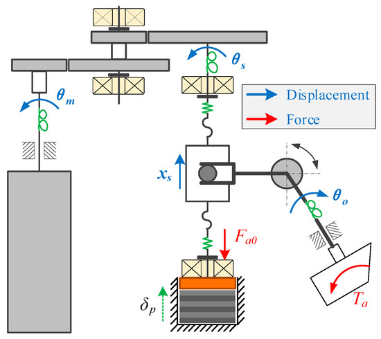
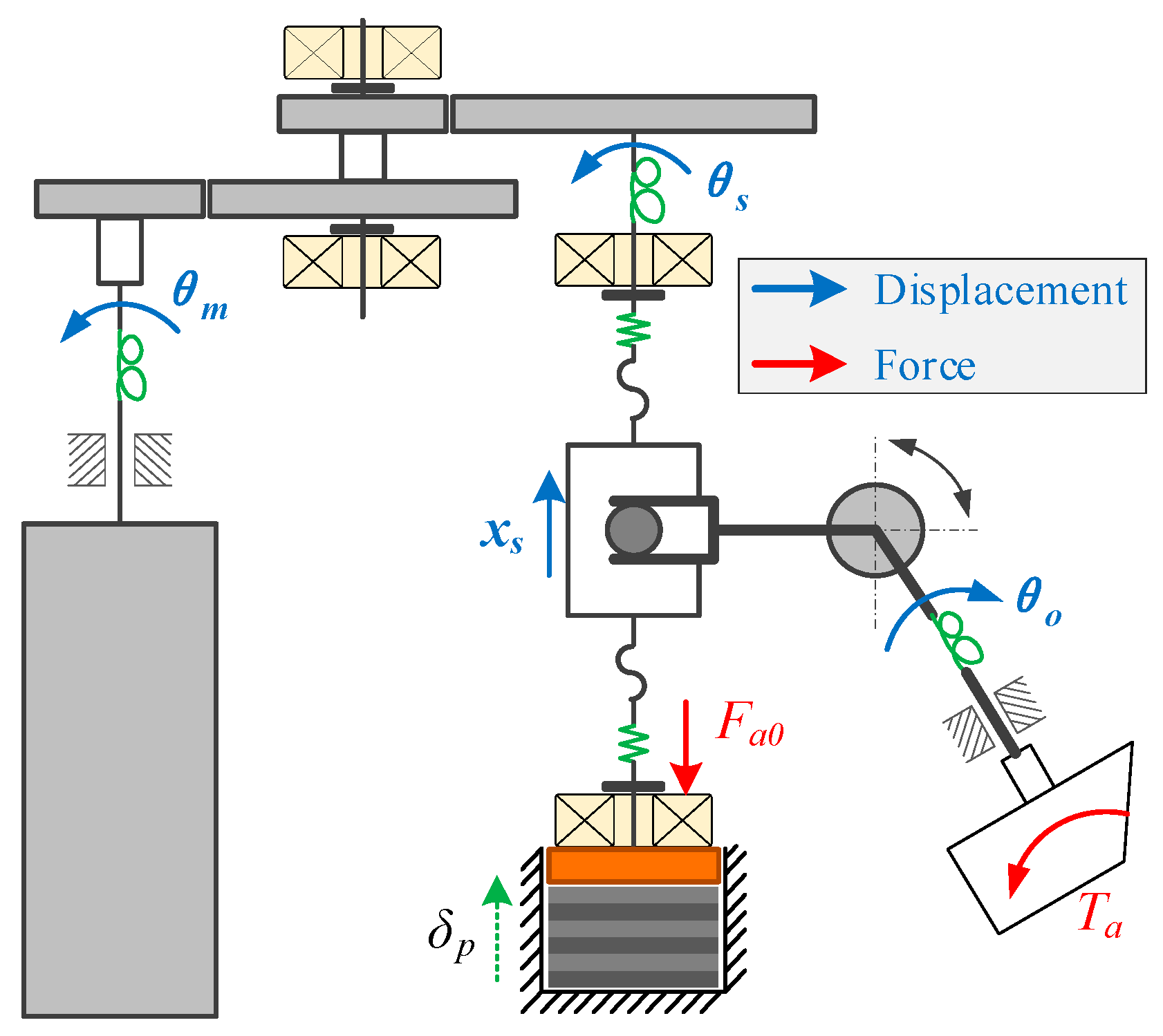
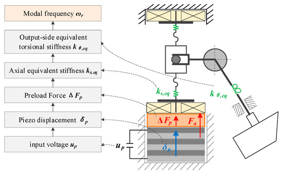
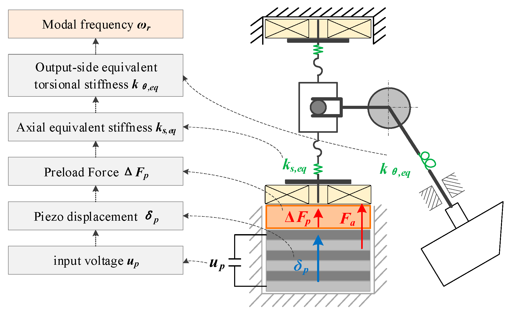
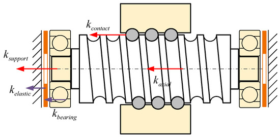
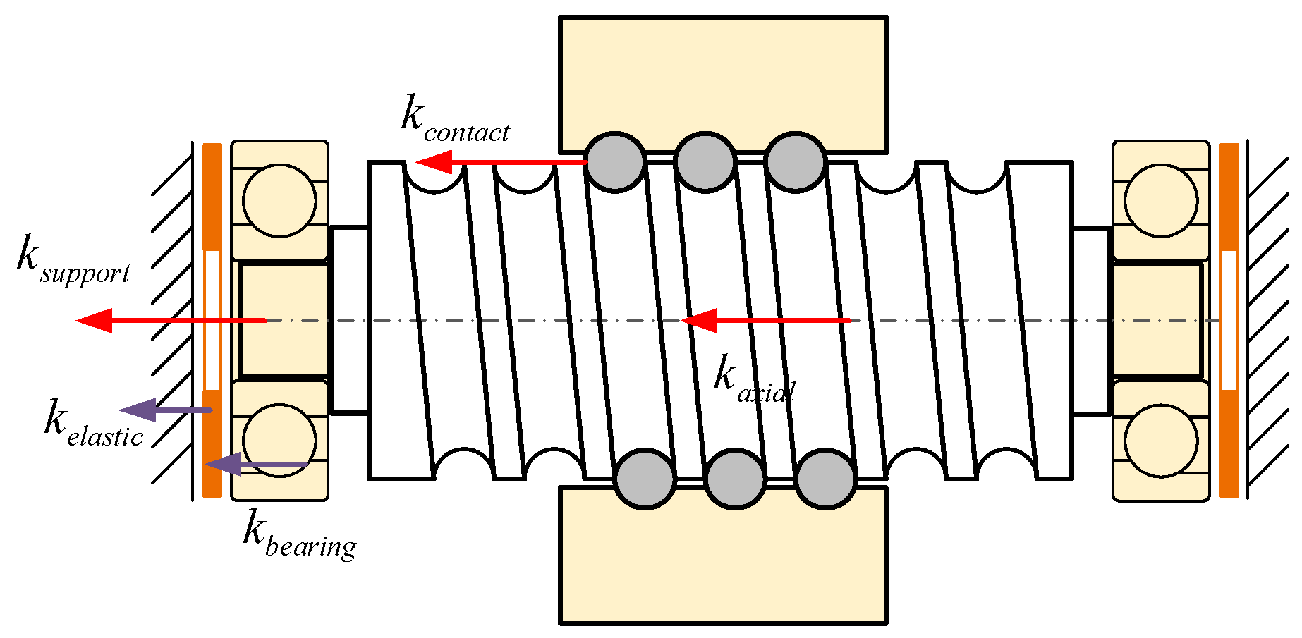
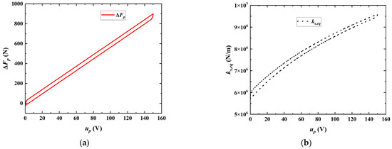
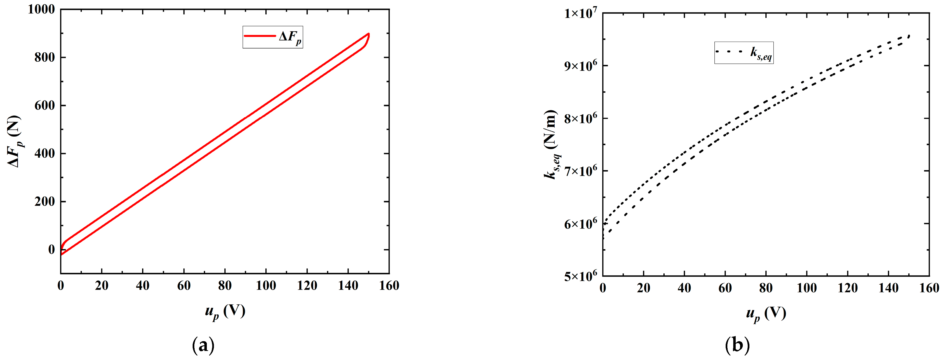
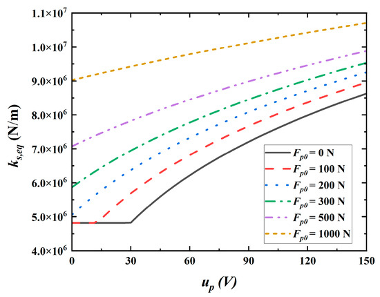
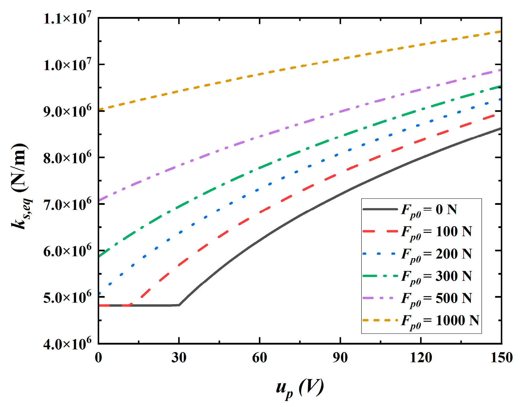
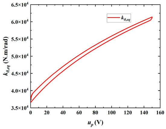
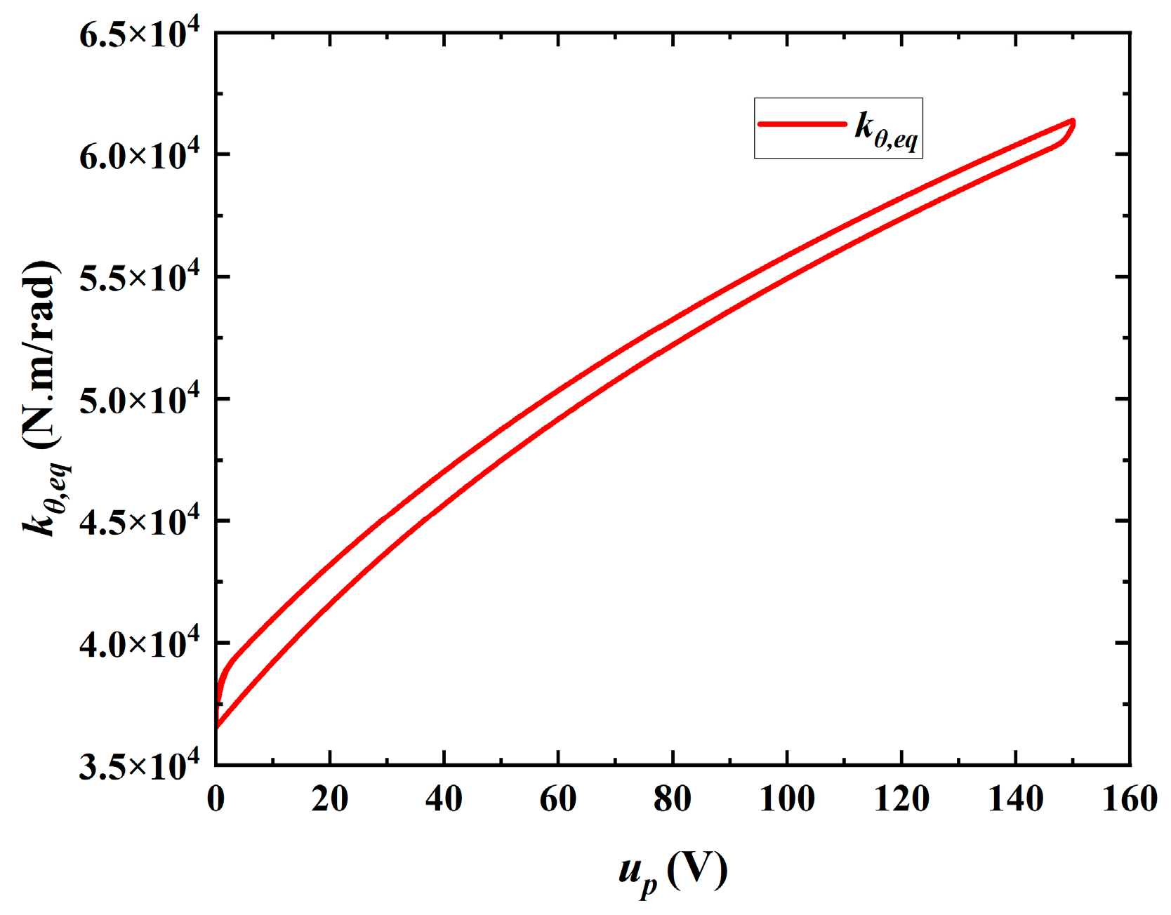
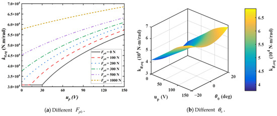
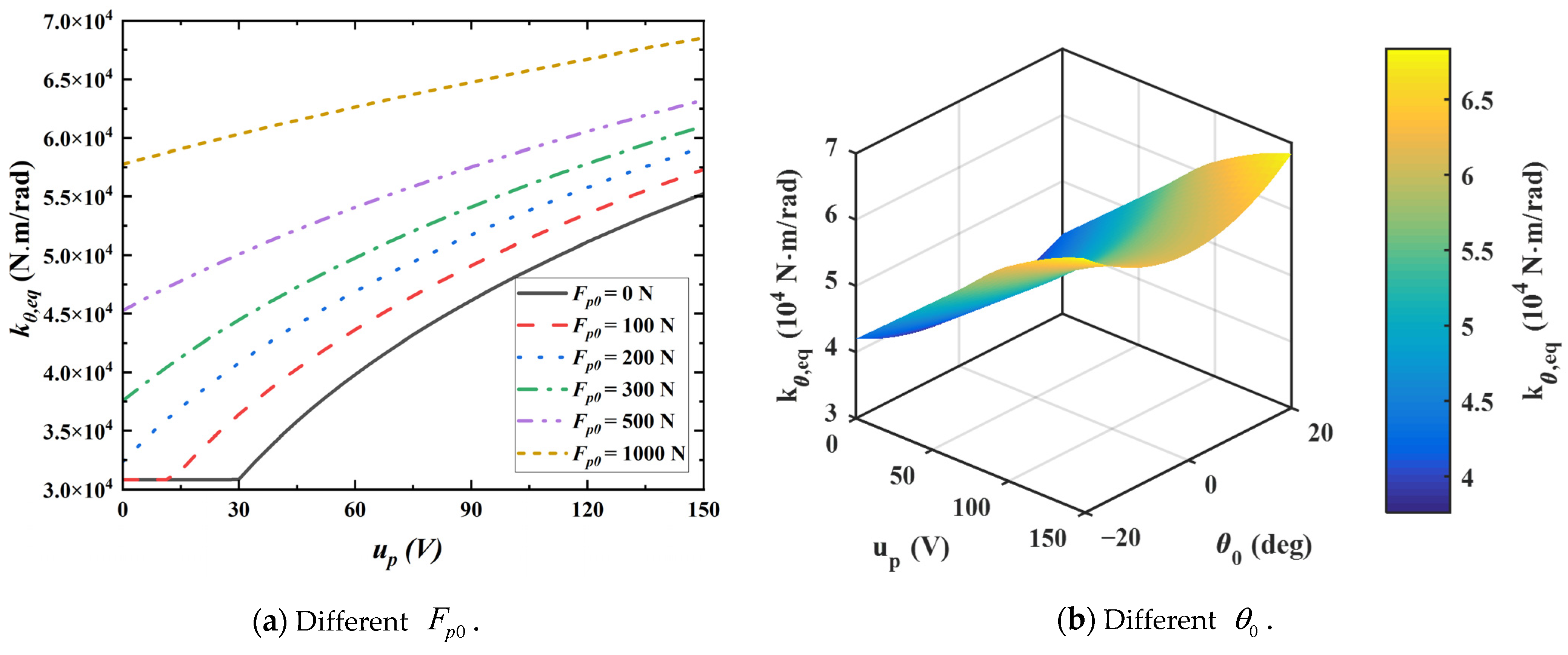
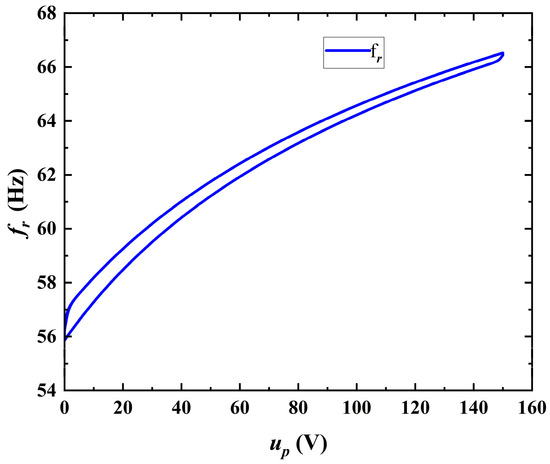
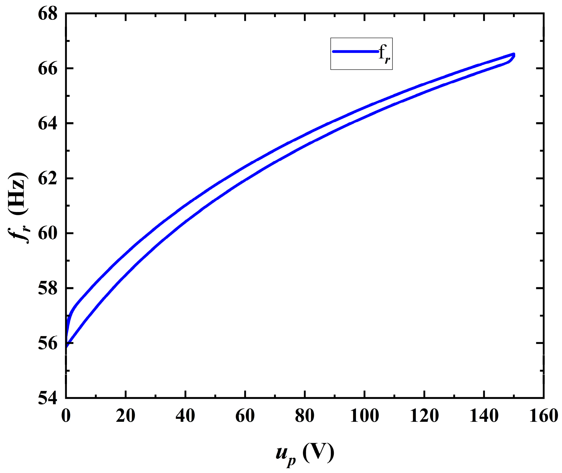
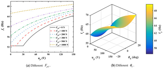
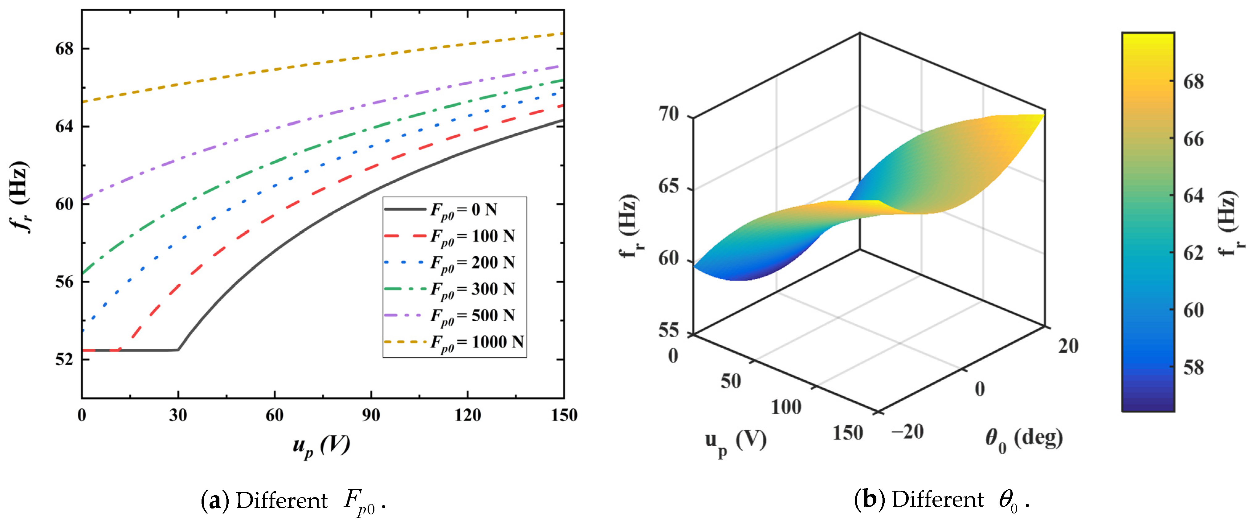
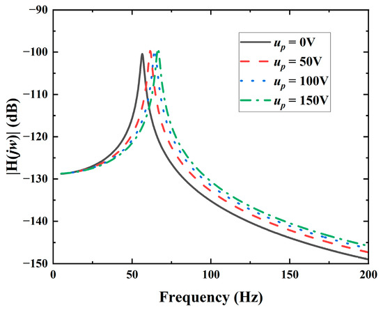
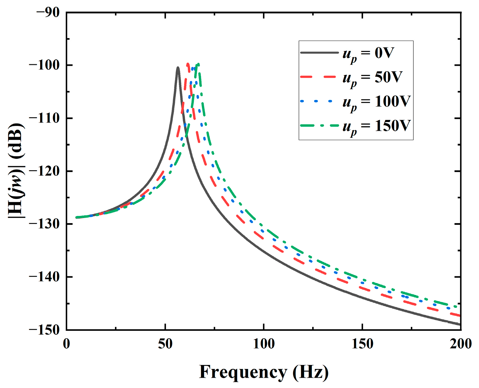
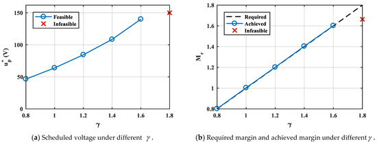
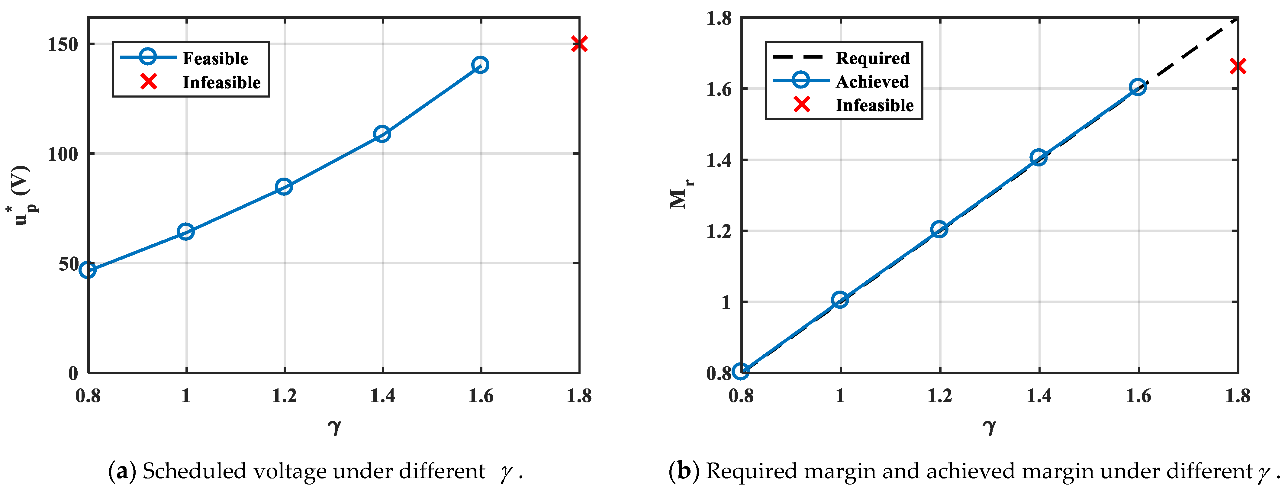
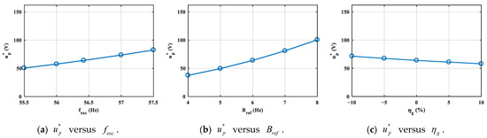
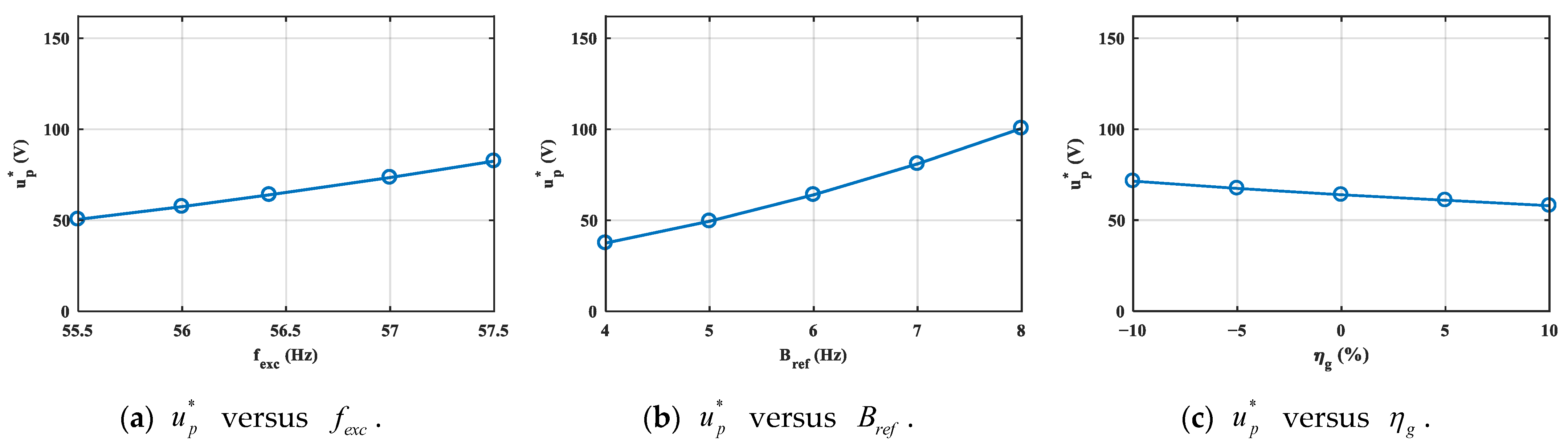
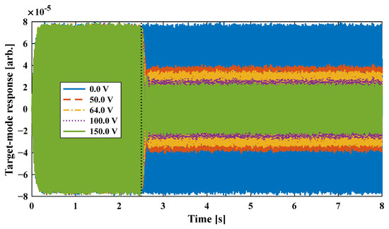
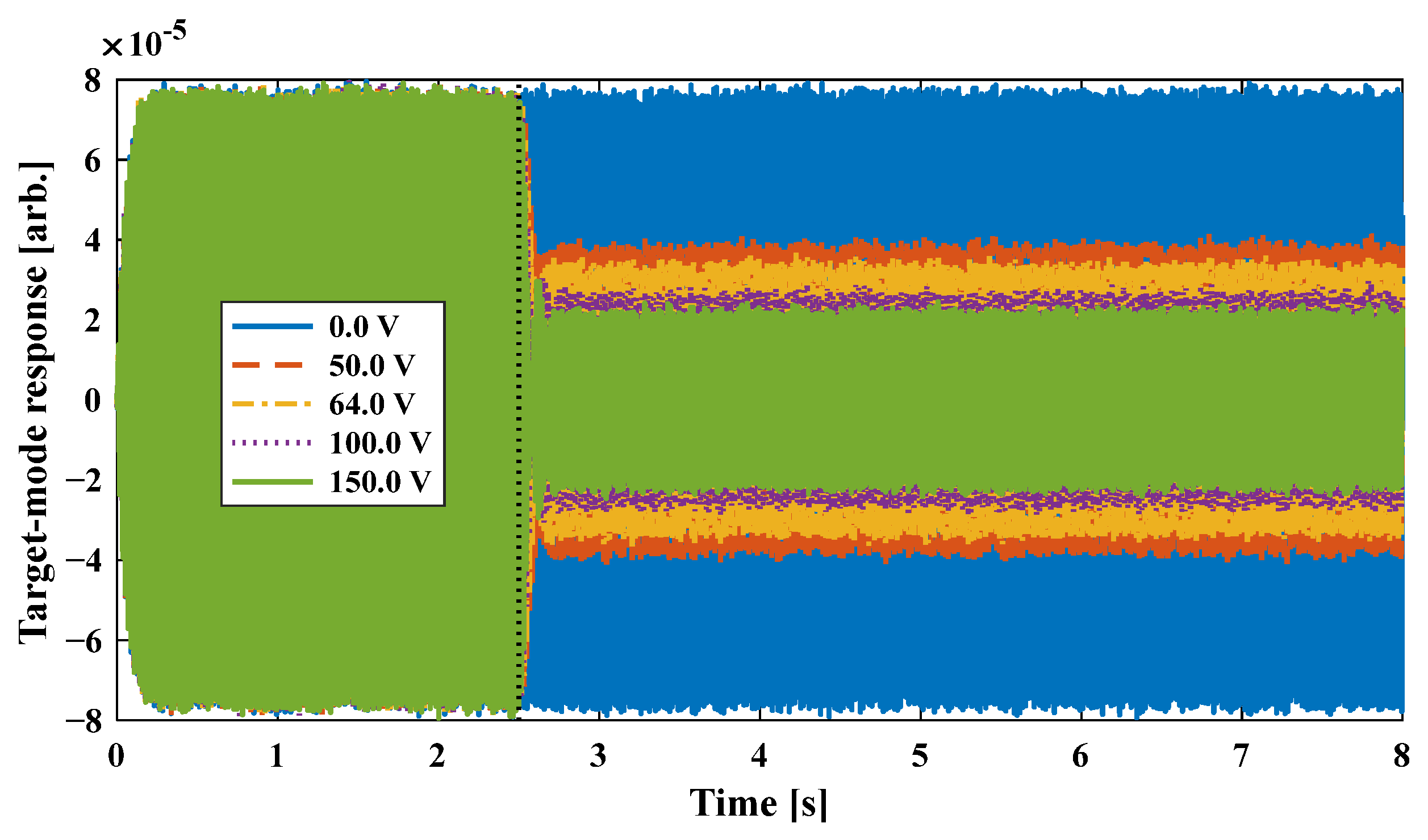

Disclaimer/Publisher’s Note: The statements, opinions and data contained in all publications are solely those of the individual author(s) and contributor(s) and not of MDPI and/or the editor(s). MDPI and/or the editor(s) disclaim responsibility for any injury to people or property resulting from any ideas, methods, instructions or products referred to in the content. |
© 2026 by the authors. Licensee MDPI, Basel, Switzerland. This article is an open access article distributed under the terms and conditions of the Creative Commons Attribution (CC BY) license.