Research on Flight Stability Assessment and Real-Time Early Warning System Based on Energy Management

Abstract

Aviation accidents during the final approach phase of transport aircraft account for nearly half of all accidents in the flight stage, with unstable approaches being a notable contributing factor. In related accident analysis research, traditional single-parameter threshold monitoring methods have shown difficulty in capturing the complex coupling relationship between kinetic energy and potential energy. This weakness results in insufficient adaptability under variable meteorological disturbances and poor risk identification. To address this limitation, this study establishes an evaluation framework based on the concepts of “energy altitude” and “balance energy, shifting the analytical focus of aircraft state variations to energy evolution. A hybrid dynamic safety boundary function is further constructed by integrating flight mechanics principles with civil aviation regulatory constraints. This boundary integrates a height attenuation mechanism, enhancing adaptability to environmental disturbances. The study adopts QAR flight data of Boeing aircraft collected at an international airport from 2015 to 2020 as the database for machine learning modeling, and selects two additional independent flight datasets under calm-air and wind-shear conditions respectively for model verification. The research results indicate that this framework provides a robust theoretical foundation for the early identification of unstable approaches and provides actionable insights for optimizing energy control strategies, thus improving flight safety under complex operational conditions. Nevertheless, the verification only relies on two groups of typical flight cases under limited meteorological conditions, which restricts the generalizability of the research conclusions. Follow-up work will expand multi-type and multi-meteorological flight samples to carry out quantitative performance evaluation and further optimize the model’s practicality under diverse operational environments.

1. Introduction

The rapid development of the global air transport industry has facilitated the growth of air traffic volume. In this context, flight safety has always been the bottom line of civil aviation operations. Notably, statistics of the International Civil Aviation Organization (ICAO) reveal a key phenomenon: The approach and landing stage accounts for approximately 4% of the entire flight process in time, but the probability of flight accident risk accounts for 49.1% of the entire flight accident risk [1]. Moreover, the unstable approach is widely considered one of the main factors inducing serious safety incidents, such as controlled flight into terrain and runway excursion. Therefore, it is useful to forecast the risk in advance by summarizing the main causes and development trends of unsafe events in the approach stage.

The civil aviation supervision system’s judgment of a stable approach mainly depends on the threshold monitoring of one flight parameter, such as altitude, CAS, descent rate, attitude, or thrust. However, it remains difficult to fully grasp the dynamic change process of aircraft energy state by exclusively focusing on one parameter. This detection method may cause all of the single monitored parameters to remain in the safe range, while the pilot’s response to abnormal energy state perception is judged to be an unstable approach. As the coupling relationship between different parameters is not fully considered in the evaluation, the evaluation results may diverge from the pilot’s real operation decision. A stable approach requires all of the relevant parameters to meet the stability standards at once. However, sometimes, cognitive biases in the operation of flight personnel can lead to an insufficient understanding of the hidden hazards of the unstable approach, leading to the inability to strictly implement stable approach requirements. Therefore, it is useful to evaluate the coupling relationship between the causes of unsafe events in the approach stage to ensure safe landing.

As early as 2006, Yi et al. [2] proposed a model based on severity classification and probability calculation, and it provided an effective paradigm for quantitative analysis of risks such as energy management failure in the approach stage. It also established an important theoretical foundation for later engineering evaluation. In 2011, Bazhenov [3] comprehensively explored the mechanism of the digital multi-rate control system on the lateral stability of the aircraft, and he pointed out that the sampling frequency of the system should be at least 50 Hz to ensure the required control accuracy. This discovery provides a key parameter basis for designing the control algorithm in the approach stage. Likewise, in 2013, Asadi et al. [4] constructed a database of trim characteristics of left-wing damaged aircraft. The discovery that the degree of artificial aircraft damage and the flight altitude at that time have a significant impact on the contraction of the approach envelope strongly promoted the exploration of targeted assessment of the risk of the damaged aircraft approach. The next year, Nasir et al. [5] evaluated the aerodynamic characteristics and flight quality of the hybrid wing-body aircraft and found that the canard configuration could improve the longitudinal static stability of the aircraft. Similarly, in 2015, Raghu et al. [6] proposed a reliability evaluation framework for a UAV actuator architecture, which showed that the redundant design could successfully reduce the probability of catastrophic failure by 40%.

In recent years, to realize the prediction and prevention of unsafe events, some researchers have evaluated the state of aircraft from the energy management perspective. In 2018, Jiao et al. [7] built an empirical model for an unstable approach below 304.8 m (1000 feet), and they found that airspeed overrun and channel deviation were the main causes of instability, revealing the profound internal relationship between approach stability and the aircraft energy state. In 2019, Hernández-Romero et al. [8] factored in environmental factors, constructed a wind field uncertainty model, quantified the specific impact of wind shear on the severity of approach conflicts, and established a novel probabilistic analysis scheme for approach risk assessment under complex meteorological conditions. In 2025, some researchers began to pay attention to the coupling effect between various driving factors. Du [9] proposed a double closed-loop sliding mode control strategy, which effectively resolved the problem of internal and external coupling in the trajectory tracking task of vertical take-off and landing aircraft. The same year, Dagal et al.’s PID controller [10] was successfully applied to the approach training simulation of Cessna 172 aircraft, and it shortened the time for the aircraft to reach a stable state by 30%.

Reducing unstable approach events and ensuring a safe landing are critical to civil aviation operation [11]. For example, existing research has shown that building a risk assessment system is the research premise, that considering the impact of the coupling relationship of various risk incentives is the key to research, and that employing energy management to complete the aircraft condition assessment is the research basis. The aircraft shifts the dynamic energy and potential energy by adjusting the engine thrust and pitch attitude. Further, the coordinated change of the two can achieve a stable and controllable decrease in the total energy during the approach and landing stage, ultimately meeting the energy conditions necessary for safe landing [12,13,14]. According to the International Civil Aviation Organization, the core of the stable approach is to maintain the controllability of the energy state [1], and the change of energy state is affected by multisource data. Therefore, to realize the accurate evaluation of the final approach stability of the aircraft, one must break through the traditional framework of single-parameter monitoring and construct a multidimensional evaluation system based on the overall energy state.

Therefore, this study aims to define core energy parameters, such as energy altitude and dynamic energy-potential energy ratio, and to establish a model to describe the dynamic evolution of energy state. The research results provide solid theoretical support for the early identification of an unstable approach, optimize the energy control strategy of critical airborne equipment, such as an automatic throttle and flight guidance system, and provide a data-driven basis for decision-making. Overall, the research results hold important theoretical value and engineering application prospects for improving the flight safety level under complex and changeable meteorological conditions.

2. Theories and Research Methods

2.1. Dynamics Analysis of the Final Approach Stage

The ICAO clearly posits that the aircraft must fly strictly along the prescribed glide path and maintain the speed within the specified range, that the vertical descent rate must not surpass −5.08 m/s (−1000 ft/min), and that the adjustment of key configurations must be completed before reaching the stable approach point [1]. However, in a real flight, pilot manipulation may cause the energy state to become out of control. For example, if the pilot decreases the dynamic energy by reducing the thrust, if the pitch angle is not adjusted in time, the potential energy decline rate may markedly exceed the dynamic energy attenuation, which can, in turn, trigger cascading effects on parameters, such as altitude, velocity, glide angle, and vertical velocity.

Further, the energy state of the aircraft is basically a comprehensive reflection of its dynamic energy and potential energy. The independent analysis of the two energies makes it difficult to effectively capture the dynamic synergy. Therefore, the study proposes “energy altitude (H_e)” and “balance energy (E_b).” The H_e was proposed by Lush, K. J. [15], and the equation can be expressed as follows:

$${\mathrm{H}}_{\mathrm{e}}=h+{\displaystyle \frac{v^2}{2g}}$$

(1)

where h denotes the current actual geometric altitude of the aircraft, v is the current speed of the aircraft, and g is the acceleration stemming from gravity. This means that the dynamic energy is turned into an equivalent altitude and superimposed with the actual geometric altitude to establish a comprehensive energy index with a unified dimension.

2.2. Energy Management and Constraints

The core control logic of energy management is to achieve an energy balance by changing the thrust and pitch angles. In earlier times, the influence of thrust and pitch angle on velocity and altitude was evaluated separately in aircraft energy management. This method often causes system failures owing to the coupling effect between parameters in complex disturbances. For example, in 1983, the Total Energy Control System (TECS) was proposed [16] and gradually recognized [17,18]. The total energy change rate was changed by adjusting the thrust, while the conversion ratio of dynamic energy and potential energy was altered by using the pitch attitude, which essentially solved the problem of the energy regulation mismatch.

Based on the quick access recorder (QAR) data of numerous accidents, the ICAO and the Civil Aviation Administration of China (CAAC) formulated constraint standards for the parameters of the final approach stage of the aircraft.

3. Construction of Stability Assessment System Based on Energy Management

3.1. Definition of Energy Parameters

For the stability evaluation of the aircraft in the final approach stage, the traditional method primarily adopts the speed- and altitude-independent monitoring mode, which has significant limitations. Owing to the strong coupling characteristics of flight parameters in the approach stage, the velocity and altitude can be linked by the conversion of dynamic energy and potential energy. External disturbances often act on velocity and altitude at the same time, making it difficult to accurately capture the essential characteristics of the energy state through a single-parameter or two-parameter independent evaluation. Therefore, H_e and E_b are employed as evaluation parameters to realize the synergistic analysis of dynamic energy and potential energy, which provides a quantitative basis for multidimensional energy state evaluation.

3.1.1. Definition of Energy Altitude

The stability of the aircraft in the final approach stage is a manifestation of the dynamic balance of dynamic energy and potential energy. Traditional research has often analyzed dynamic energy and potential energy independently, which cannot reflect the synergistic relationship. Therefore, this study leverages the idea of unified control of total energy to convert dynamic energy into an equivalent altitude. H_e can be obtained by adding the equivalent altitude to the actual altitude, while the aircraft’s total energy reserve can be intuitively characterized by one parameter.

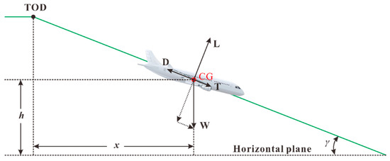
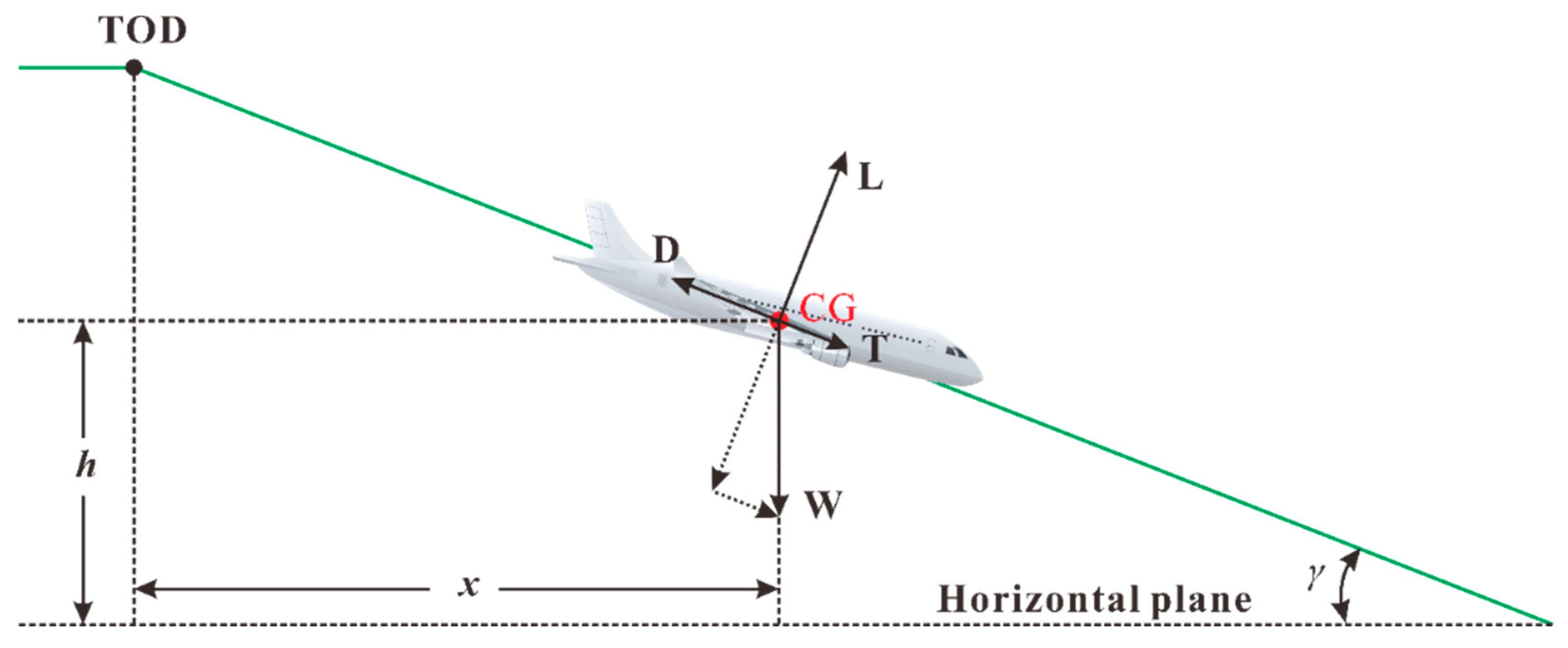
The key aircraft descent parameters are listed in Table 1. The forces of the aircraft are shown in Figure 1. The green solid line denotes the trajectory, TOD denotes the top of descent, and CG represents gravity’s center.

Table 1. Parameters of aircraft descent.

Name	Symbol	Unit
Horizontal distance	x	m
The geometric altitude from the horizontal plane	h	m
Track angle (the angle between the track and the horizontal plane)	γ	rad
Gravity	W	N
Thrust	T	N
Drag	D	N
Lift	L	N
True air speed	VT	m/s
Wind speed	VW	m/s

Figure 1. The motion force of the aircraft descending.

The aircraft is regarded as a particle, and its kinematic equation can be expressed as follows:

$$\left\{\begin{array}{c}{\displaystyle \frac{dx}{dt}}={\mathrm{V}}_T\cos \gamma +{\mathrm{V}}_{Wx}\\ {\displaystyle \frac{dh}{dt}}={\mathrm{V}}_T\sin \gamma +{\mathrm{V}}_{Wh}\\ {\displaystyle \frac{d{\mathrm{V}}_T}{dt}}={\displaystyle \frac{\mathrm{T}-\mathrm{D}}{m}}+g\sin \gamma \end{array}\right.$$

(2)

where m is the mass of the aircraft (kg), g is the gravitational acceleration (9.81 m/s²), t is the flight time (s), V_Wx denotes the decomposition of the wind speed in the horizontal direction, and V_Wh represents the decomposition of the wind speed in the vertical direction. According to the above equation, the following can be obtained:

$$\mathrm{T}=({\displaystyle \frac{{\dot{\mathrm{V}}}_T}{g}}-\gamma )mg+\mathrm{D}$$

(3)

The total energy E_T of the aircraft can be expressed as the sum of dynamic energy E_D and gravitational potential energy E_P:

$${\mathrm{E}}_T={\mathrm{E}}_D+{\mathrm{E}}_P={\displaystyle \frac{1}{2}}m{\mathrm{V}}_T^2+mgh$$

(4)

To achieve dimensional unification, the total energy is equivalent to the “altitude” form. Assuming that the total energy is completely converted into potential energy, the total unit quality energy can be obtained as follows:

$${\mathrm{E}}_T={\displaystyle \frac{{\mathrm{V}}_T^2}{2g}}+h$$

(5)

Here, H_e can reflect the total energy reserve state of the aircraft through one parameter (equivalent altitude). If the energy altitude is high, the total energy is present in excess, which may lead to an excessive touch-down speed. If, however, the energy altitude is low, the total energy is insufficient, and there may be risks such as poor anti-disturbance ability.

3.1.2. Total Energy Change Rate

The derivation of Equation (5) can be obtained as follows:

$${\dot{\mathrm{E}}}_T={\mathrm{V}}_T{\displaystyle \frac{{\dot{\mathrm{V}}}_T}{g}}+\dot{h}$$

(6)

As $\dot{h}={\mathrm{V}}_T\sin \gamma$, one can bring it into Equation (6) to get the following:

$${\displaystyle \frac{{\dot{\mathrm{E}}}_T}{{\mathrm{V}}_T}}={\displaystyle \frac{{\dot{\mathrm{V}}}_T}{g}}+\sin \gamma$$

(7)

This is because the descent angle is small. In the instrument landing system (ILS) rule, the standard descent angle is set to 0.5236 rad (3 degrees). Thus, $\sin \gamma \approx \gamma$ can be considered. Therefore, Equation (7) can be rewritten as follows:

$${\displaystyle \frac{{\dot{\mathrm{E}}}_T}{{\mathrm{V}}_T}}\approx {\displaystyle \frac{{\dot{\mathrm{V}}}_T}{g}}+\gamma$$

(8)

Bring Equation (3) into Equation (8):

$$\mathrm{T}-\mathrm{D}=mg\left({\displaystyle \frac{{\mathrm{V}}_T}{g}}+\gamma \right)$$

(9)

When the aircraft is in normal flight, the weight change primarily stems from the reduction of fuel.

Thus, the mass of the aircraft is almost unchanged in a short period of time, and mg is considered to be a constant. ${\displaystyle \frac{{\dot{\mathrm{V}}}_T}{g}}$ can be used to characterize the changing kinetic energy rate. Alternatively, γ (or sin γ) can be used to characterize the changing rate of gravitational potential energy. By changing the thrust, the total energy can be directly regulated, while the distribution ratio of kinetic energy and potential energy can be modified by changing the track angle γ.

3.1.3. Definition of Balanced Energy

The balanced distribution of kinetic energy and potential energy during flight is the key factor determining the approach operation. Through the quantitative analysis of the equilibrium degree of kinetic energy and potential energy distribution, it provides an intuitive and real-time reference for pilots, which can help improve the safety and accuracy of approach operation.

E_b (balanced energy) is defined as the difference between potential energy and kinetic energy, which is expressed as follows:

$${\mathrm{E}}_{\mathrm{b}}={\mathrm{E}}_P-{\mathrm{E}}_D$$

(10)

where E_P = mgh denotes gravitational potential energy in joules (J), and E_D = ${\displaystyle \frac{1}{2}}m{\mathrm{V}}_T^2$ denotes kinetic energy in joules (J). Therefore, E_b carries the unit of joule (J).

The E_b is used to quantify the distribution equilibrium of dynamic energy and potential energy. When E_b approaches zero, the distribution of dynamic energy and potential energy is in an equilibrium state. If E_b > 0, potential energy is dominant, representing a higher altitude or lower velocity. If E_b < 0, kinetic energy is dominant, representing a lower altitude or higher speed. If there is too much kinetic energy, it is necessary to convert the excess kinetic energy into potential energy by increasing the pitch angle.

The time-changing rate of balanced energy ${\dot{\mathrm{E}}}_{\mathrm{b}}$ (unit: watt, W) is derived by differentiating both sides of Formula (10) with respect to flight time t:

$${\dot{\mathrm{E}}}_{\mathrm{b}}={\displaystyle \frac{d{E}_P}{dt}}-{\displaystyle \frac{d{E}_D}{dt}}=mg\dot{h}-m{\mathrm{V}}_T{\dot{\mathrm{V}}}_T$$

(11)

By bringing $\dot{h}={\mathrm{V}}_T\sin \gamma$ into the above formula, one obtains the following:

$${\dot{\mathrm{E}}}_{\mathrm{b}}=mg{\mathrm{V}}_{T}sin\gamma -m{\mathrm{V}}_T{\dot{\mathrm{V}}}_T$$

(12)

Each term on the right side has a unit of watt (W), representing the instantaneous changing rate of energy partition.

Note that the mass m and true airspeed ${\mathrm{V}}_T$ of the aircraft are nearly constant over a short period. To eliminate dimensional interference, divide the right side of the Formula (12) by $mg{\mathrm{V}}_T$. The dimensionless quantity $sin\gamma -{\displaystyle \frac{{\dot{\mathrm{V}}}_T}{g}}$ is proportional to the balance energy change rate ${\dot{\mathrm{E}}}_{\mathrm{b}}$. Which can be expressed as the following:

$${\dot{\mathrm{E}}}_{\mathrm{b}}\propto \left(sin\gamma -{\displaystyle \frac{{\dot{\mathrm{V}}}_T}{g}}\right)$$

(13)

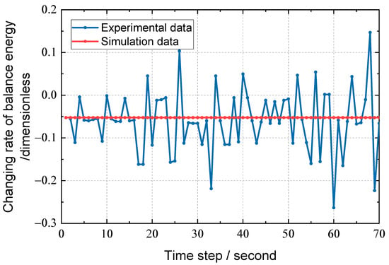
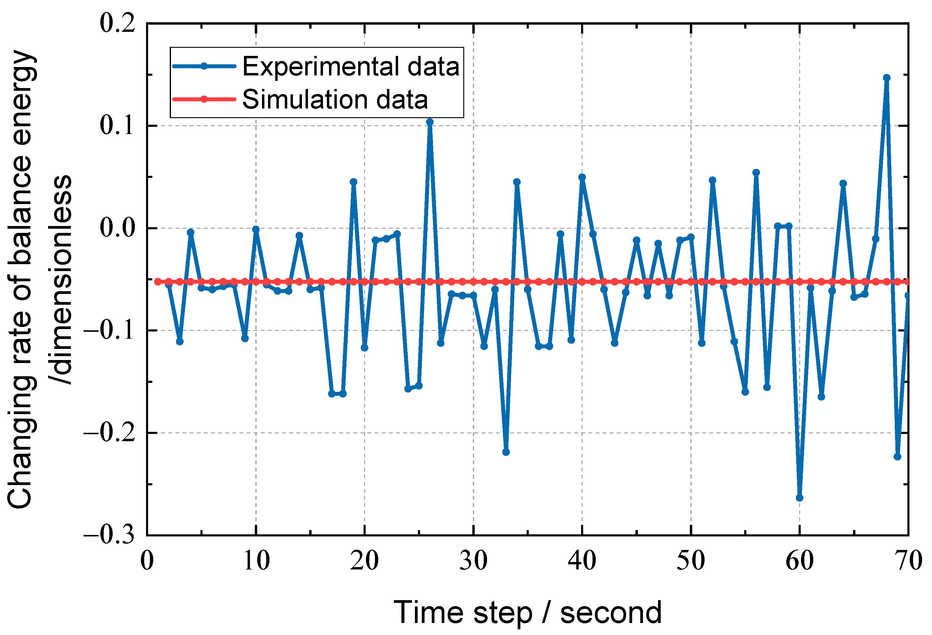
Therefore, $sin\gamma -{\displaystyle \frac{{\dot{\mathrm{V}}}_T}{g}}$ (a dimensionless value) will be used to reflect the trend of ${\dot{\mathrm{E}}}_{\mathrm{b}}$ in subsequent analysis, as shown in Figure 2. Taking the standard 0.5236 rad (3 degrees) glide angle, and 77.17 m/s (150 knots) air speed and no wind condition as the standard. In Figure 2, the vertical axis is a dimensionless quantity. The figure shows the comparison diagram of the balance energy changing rate curve between the measured and standard state of the last 304.8 m (1000 feet) approach stage of the aircraft. One can find that the standard curve maintains a stable and regular trend throughout the process, while the measured data can respond to the dynamic change of energy change rate in real time. The fluctuation frequency of ${\dot{\mathrm{E}}}_{\mathrm{b}}$ is higher than the traditional parameters, such as speed and altitude, which can capture the abnormal energy distribution in advance and provide a timelier decision-making basis for pilots.

Figure 2. Changing rate of balance energy.

3.2. Construction of Safety Boundary Function

As the key constraint of the evaluation system, the design of the safety boundary function is paramount. This study employs the basic theory of flight mechanics, combined with civil aviation regulations and standards, to construct a dynamic boundary function. The function accurately establishes the safety boundary of aircraft energy state through multi-parameter cooperative coupling and adaptive adjustment mechanism, and it offers a reliable basis for the approach stability evaluation.

3.2.1. Static Boundary Restrictions Based on Civil Aviation Regulations

The core goal of the final approach is to maintain a stable airspeed, a 0.5236 rad (3 degrees) sliding angle, and a reasonable energy state, which ultimately achieves a safe touchdown. The energy state of this stage must meet the “double decreasing” rule; that is, the total energy decreases continuously with the decrease of altitude, while the distribution of kinetic energy and potential energy must be balanced. Therefore, the design of the boundary function should focus on core parameters such as energy altitude and balanced energy, and it should factor in the dynamic stability requirements and actual constraints.

The static boundary is the “bottom line constraint” of the safety envelope. In other words, its design should strictly adhere to the civil aviation regulations and flight mechanics principles to ensure the safety of the energy state under ideal conditions. Per the relevant requirements of the Flight Standards Division of the Civil Aviation Administration of China, the target approach speed (V_app) is used as the core reference, and the actual flight speed must be accurately maintained in the range of V_app − 2.57 to V_app + 5.14 m/s (V_app − 5 to V_app + 10 knots). To ensure that the pilot’s operating margin and re-flight energy reserve, the decline rate in the final approach stage must be controlled within −5.08 m/s (−1000 ft/min), and sufficient adjustment time should be reserved for the pilot.

In the final approach stage, the setting of the energy altitude boundary is critical to ensuring safe landing. Taking the runway entrance as the key node, the safety constraints are constructed based on the principle of energy conservation. When the aircraft reaches the runway entrance, the total energy must meet the requirements of safe landing, and the safety lower limit of energy altitude is obtained accordingly. To ensure the smooth landing of the aircraft from the energy point of view and ensure that the aircraft has the appropriate energy reserve at the end of the approach, we employ the following formula:

$${\mathrm{E}}_{T,thr}={\displaystyle \frac{1}{2}}mTA{S}_{thr}^2+mg{h}_{thr}$$

(14)

where ${\mathrm{E}}_{T,thr}$ is the total energy of the runway entrance, $TA{S}_{thr}$ is the allowable vacuum speed of the runway entrance, and $h_{thr}$ is the allowable altitude of the runway entrance.

The initial safety envelope is an energy static boundary (${\mathrm{E}}_{static}$) defined based on the physical model. To match the operation logic of “lower altitude and stricter energy control” in the approach stage, the altitude attenuation function $f(h)$ is established to dynamically adjust the static boundary:

$$f(h)=\exp \left(-{\displaystyle \frac{h_{ref}-h_{x,y,z}}{h_{ref}}}\right)=\exp \left({\displaystyle \frac{h_{x,y,z}}{h_{ref}}}-1\right)$$

(15)

Here, $h_{ref}$ increases the stable altitude of 304.8 m (1000 feet) based on the airport elevation, which is taken as a reference point for comparison with the current actual flight altitude. Moreover, $h_{x,y,z}$ denotes the current position altitude. Further, the range of ${\mathrm{E}}_{static}$ is as follows:

$${\mathrm{E}}_{static}\in \left\{\left[{\mathrm{E}}_{T,tre}-\Delta {\mathrm{E}}_{\min }\times f\left(h\right)\right],\left[{\mathrm{E}}_{T,tre}+\Delta {\mathrm{E}}_{\max }\times f\left(h\right)\right]\right\}$$

(16)

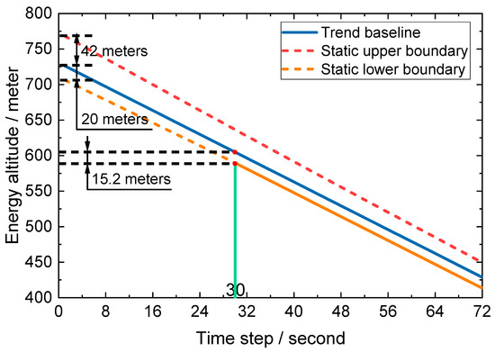
where ${\mathrm{E}}_{T,tre}$ denotes the trend baseline fitted according to the global energy altitude. $\Delta {\mathrm{E}}_{\min }$ signifies the minimum energy corresponding to the lower limit of energy altitude fluctuation. When the speed falls below the standard 2.57 m/s (5 knots), the corresponding altitude after conversion to equal energy potential energy is less than 20 m (65.62 feet). $\Delta {\mathrm{E}}_{\max }$ represents the maximum energy corresponding to the upper limit of energy altitude fluctuation; that is, the speed exceeds the standard 5.14 m/s (10 knots), while the corresponding altitude after conversion to equal energy potential energy is 42 m (137.80 feet).

In higher airspace, the flight trajectory is difficult to be affected by obstacles. As such, the upper boundary of energy altitude is wide, which can contain the natural fluctuation of energy during normal flight. As the trajectory of the aircraft declines, the tolerable fluctuations at the lower altitude boundary continue to narrow in an exponential decay fashion. This function design can lead to the smooth transition of the boundary and effectively avoid the judgment deviation due to the sudden change of the boundary.

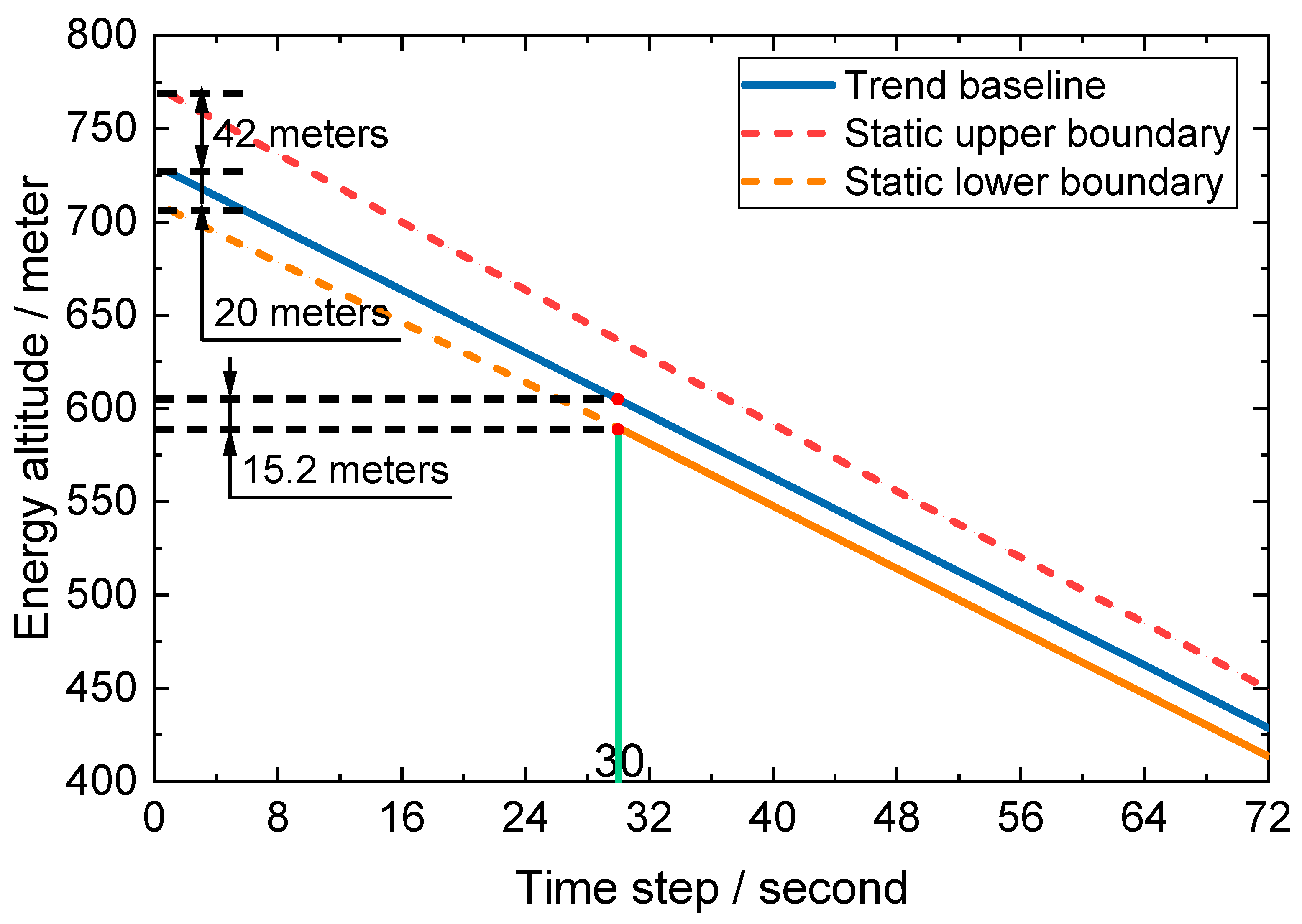
Figure 3 shows the trend baseline ${\mathrm{H}}_{T,tre}$ and its static boundary diagram. The initial position of the static upper boundary is 42 m (137.80 feet) higher than the trend line, while the initial position of the static lower boundary is 20 m (65.62 feet) lower than the trend line. Over time, the upper boundary gradually approaches the trend baseline, while the distance from the lower boundary to the trend line reduces to 15.2 m (50 feet) within 30 s and remains parallel to the trend baseline after 30 s. The change trend of the range between the static upper boundary and the lower boundary can be divided into two parts: The first 30 s are the dynamic narrowing stage. After 30 s, the parallel descent stage begins, which provides a reference frame for the energy altitude monitoring range during the aircraft approach.

Figure 3. Trend Baseline and Static Boundary Diagram.

3.2.2. Data-Driven Dynamic Boundary Correction

The static boundary establishes the energy range in the ideal scene. However, in real operation, complex and changeable meteorological conditions often arise, so the static boundary is difficult to adapt to the dynamic fluctuation of energy. Therefore, this study employs the QAR data of Boeing aircraft at an international airport from 2015 to 2020 as the research object, deeply mines the key information, and proposes a dynamic boundary correction strategy combining energy altitude and equilibrium energy. The sliding window statistical technology is utilized to capture the data characteristics, and the trend analysis method is employed to optimize the safety envelope contour, ensuring that the boundary setting can better adapt to the complex environmental conditions and improve the environmental adaptability and practical application value of the evaluation system.

1. Data pre-processing

To accurately analyze the characteristics of energy data, the linear fitting method is employed to extract the trend baseline ${\mathrm{H}}_{T,tre}$, which can effectively separate the long-term trend and short-term fluctuation in the data. By calculating the residual ${\mathrm{H}}_{T,res}$, we can visually present the short-term deviation of the energy altitude relative to the ideal trend. This data processing avoids the interference of trend factors on quantile calculation and ensures the accuracy of subsequent analysis. The residual equation is as follows:

$${\mathrm{H}}_{T,res}={\mathrm{H}}_{T,thr}-{\mathrm{H}}_{T,tre}$$

(17)

The Z-score standardization of the residuals can eliminate the influence of the dimensional differences of different parameters, allowing the parameters to be compared and analyzed at a unified scale, which lays a foundation for the later construction of the dynamic boundary correction model. The standardized treatment is as follows:

$${\mathrm{X}}_{\mathrm{norm}}={\displaystyle \frac{\mathrm{X}-\mu \mathrm{X}}{\sigma \mathrm{X}}},\left(\mathrm{X}\in \{{\mathrm{H}}_{T,res},{\mathrm{E}}_b\}\right)$$

(18)

where X represents any parameter that is standardized, and ${\mathrm{X}}_{norm}$ represents the standardized parameter. Finally, μX and σX are the mean and standard deviation of the parameter X, respectively.

2. Dynamic boundary correction method

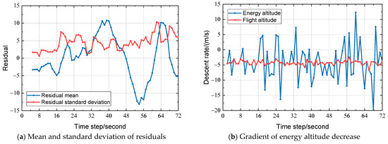
(1) A sliding window with a length of 5 s is employed to extract the following features:

• Residual mean value μ_res: The average level of energy fluctuations in the window, which reflects short-term fluctuations, for anomaly detection.
• Residual standard deviation σ_res: This measures the dispersion za5445 of energy fluctuation. The larger the standard deviation is, the more violent the fluctuation.
• Energy altitude drop rate β: This metric ensures that the drop rate meets the energy gradient requirements for stable approach:

$$\beta ={\displaystyle \frac{{\mathrm{H}}_{e,end}-{\mathrm{H}}_{e,start}}{t_{end}-t_{start}}}$$

(19)

where ${\mathrm{H}}_{e,start}$ represents the energy altitude at the final moment, ${\mathrm{H}}_{e,end}$ is the energy altitude at the initial moment, $t_{end}$ is the final moment, and $t_{start}$ is the initial moment.

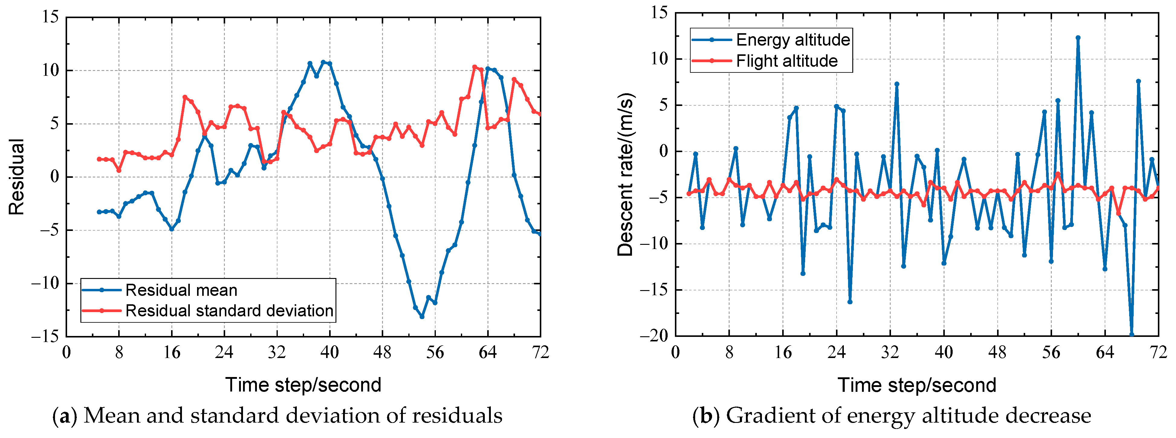
The extracted data are shown in Figure 4. Figure 4a shows the residual mean and standard deviation at different times, while Figure 4b shows the rate of decrease in energy altitude and flight altitude at different times.

Figure 4. Sliding Window Feature Extraction.

(2) Dynamic boundary adjustment rules:

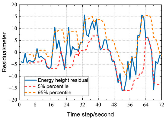
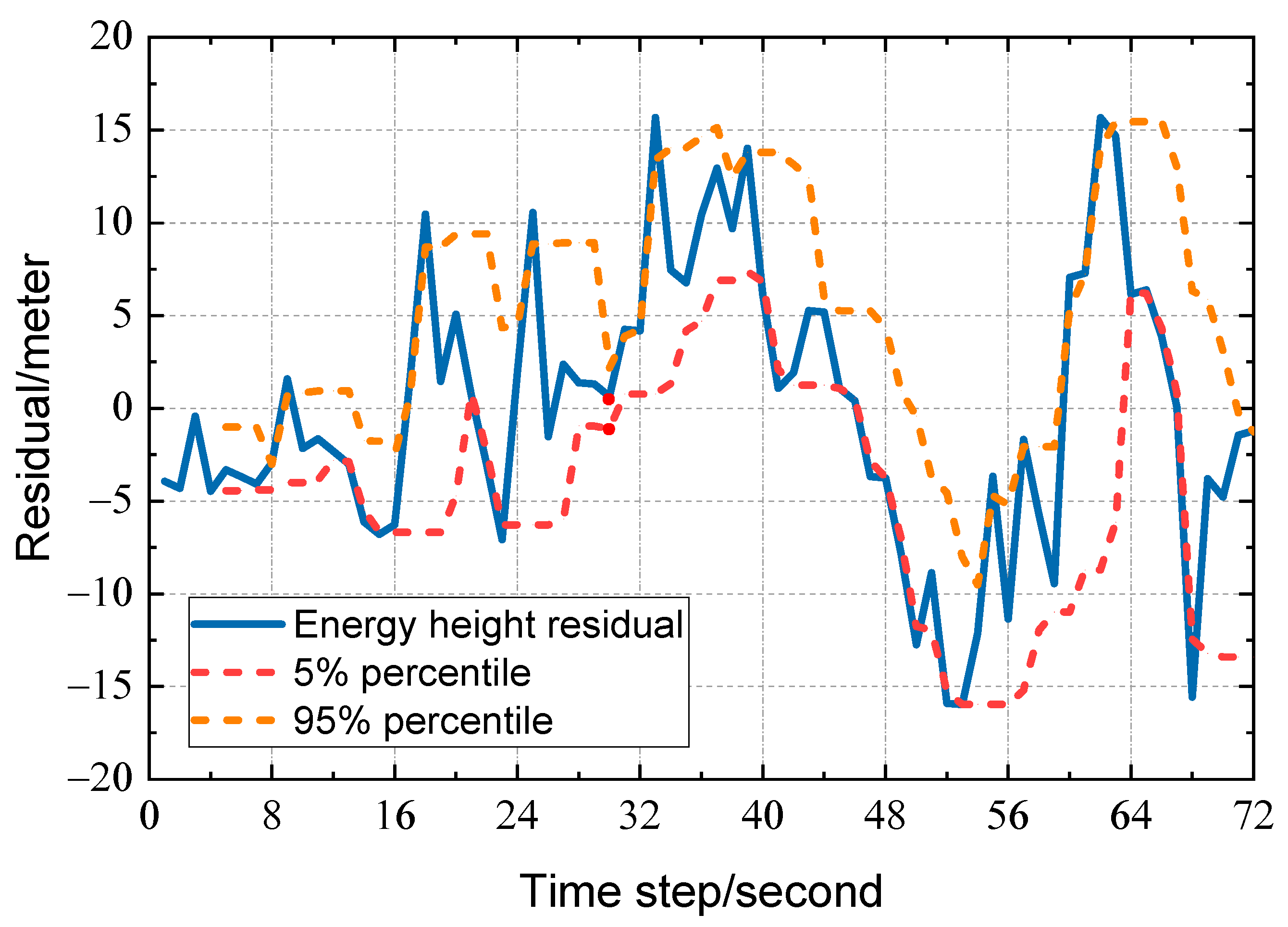
Calculate the 5% and 95% quantiles of the residuals within the window based on the residual quantiles, using the following equation:

$$\left\{\begin{array}{c}{\mathrm{H}}_{T,upper}={\mathrm{H}}_{T,tre}+(Q_{0.95}+1.5{\sigma }_{res})\times f(h)\\ {\mathrm{H}}_{T,lower}={\mathrm{H}}_{T,tre}+(Q_{0.05}-1.5{\sigma }_{res})\times f(h)\end{array}\right.$$

(20)

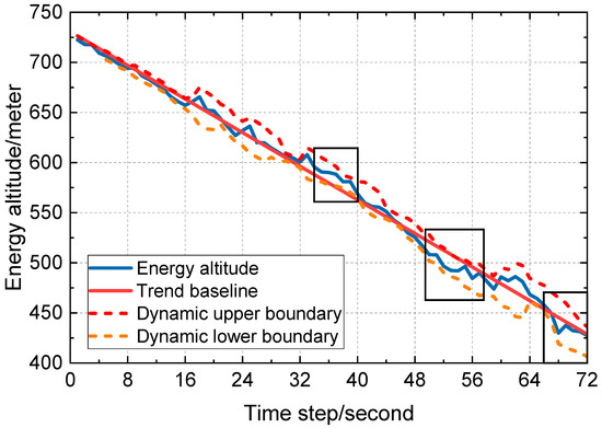
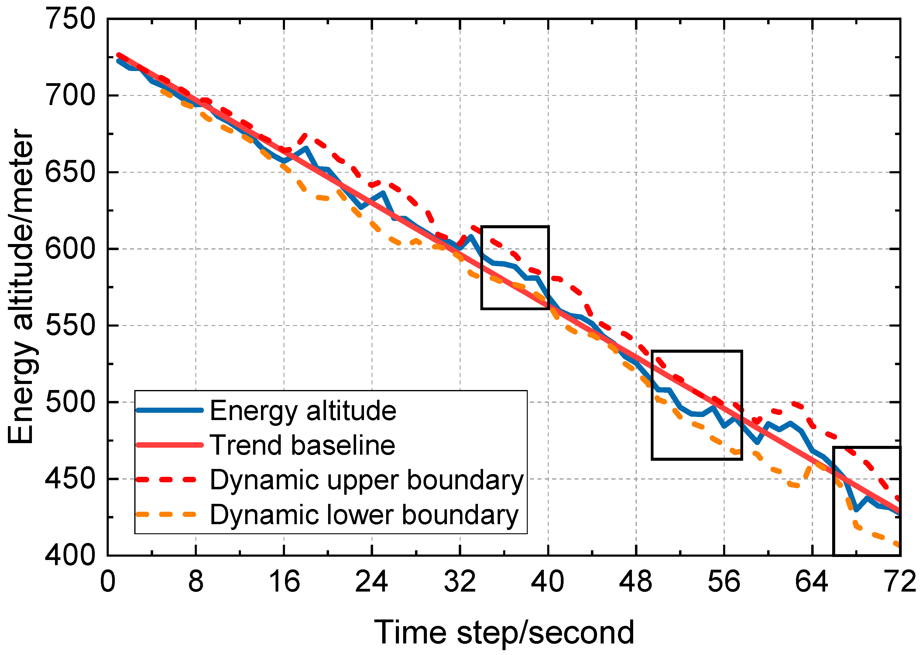
Here, Q_0.05 and Q_0.95 are standard fluctuation ranges for capturing residuals covering 90% of the data. ${\sigma }_{res}$ denotes a 1.5-fold safety margin for the residuals. The simulation results show that the anomaly timestamps output by this model are the closest to the actual anomaly timestamps in real flight data, effectively avoiding false alarms. ${\mathrm{H}}_{T,upper}$ and ${\mathrm{H}}_{T,lower}$ are the static upper boundary and static lower boundary, respectively. ${\mathrm{H}}_{T,tre}$ represents the energy altitude descent curve fitted based on actual flight data. The dynamic margin is shown in Figure 5. The window size in Figure 5 is 5 s. After calculating the residuals, we arrange them in ascending order and extract the 5% and 95% quantiles.

Figure 5. The 5% and 95% quantiles of residuals within the window.

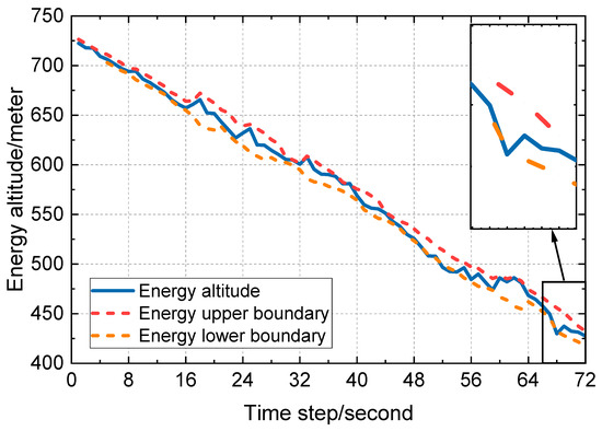
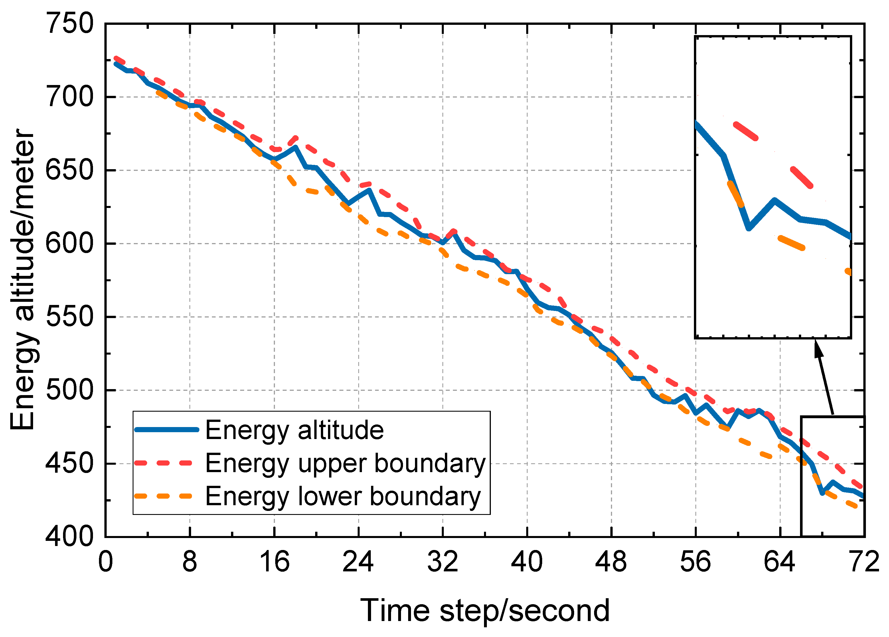
Balanced energy triggers tighten the boundary mechanism: If the difference between the balance energy changing rate ${\dot{\mathrm{E}}}_{\mathrm{b}}$ and the standard value within the window exceeds 0.15 rad (8.59 degrees) and lasts for 2 s, it is determined that the energy distribution is imbalanced. At this time, the tightening boundary Formula (21) will be triggered, and the dynamic boundary will be tightened to provide an alert of an abnormal energy distribution in advance. The enlarged region shown in Figure 6. Through offline experimental investigations, we find that when the threshold is set below 0.15 rad, the model exhibits excessive sensitivity, causing the dynamic boundary to become overly narrow and leading to a high rate of false alarms. Conversely, when the threshold exceeds 0.15 rad, the model suffers from insufficient sensitivity, resulting in delayed boundary adjustments that fail to meet the objective of “early warning.” Consequently, this empirical value of 0.15 rad was adopted in this paper. Subsequent validation using flight data confirmed that this threshold enables precise triggering of the tightened boundary mechanism, effectively identifying potential energy distribution imbalances.

$${\mathrm{H}}_{T,upper}\leftarrow {\mathrm{H}}_{T,upper}\times 0.95,{\mathrm{H}}_{T,upper}\leftarrow {\mathrm{H}}_{T,upper}\times 1.05$$

(21)

Figure 6. Data-driven dynamic boundaries.

This mechanism improves the accuracy of early warning by balancing the continuous anomaly recognition of energy and focusing boundary adjustments on energy allocation rather than fluctuation amplitude.

3.3. Comparative Experiment

3.3.1. Mixed Boundary Method

This study uses flight records of a B777 aircraft collected at an international airport on 5 April 2015 to carry out experiments. The complete dataset covers all key flight parameters throughout the final approach phase, including airspeed, descent rate, fan speed N1 and energy altitude, with a sampling interval of 1 s. Multiple disturbance scenarios are contained within the records, namely, routine weather, light turbulence and mild wind shear, which fully reflect typical energy fluctuation patterns during descent and approach. No sensor malfunctions or missing critical values were detected in the records, and sampling frequency as well as measurement precision of velocity, altitude and other vital parameters fully comply with ICAO specifications. To avoid data leakage issues, this portion of data is used as independent data outside of the machine learning dataset.

The data preprocessing steps are as follows: The 3σ criterion is used to eliminate abnormal points caused by sensor noise. The core parameters, such as energy altitude and balance energy, are standardized by the Z-score to ensure the consistency of model input. Further, continuous data from the altitude range of 126.49–431.29 m (415–1415 feet) are extracted to focus on the key stages below the stable altitude.

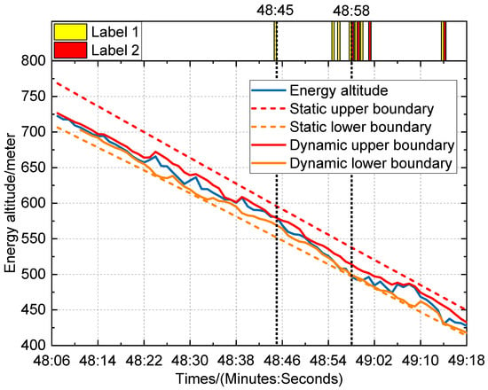
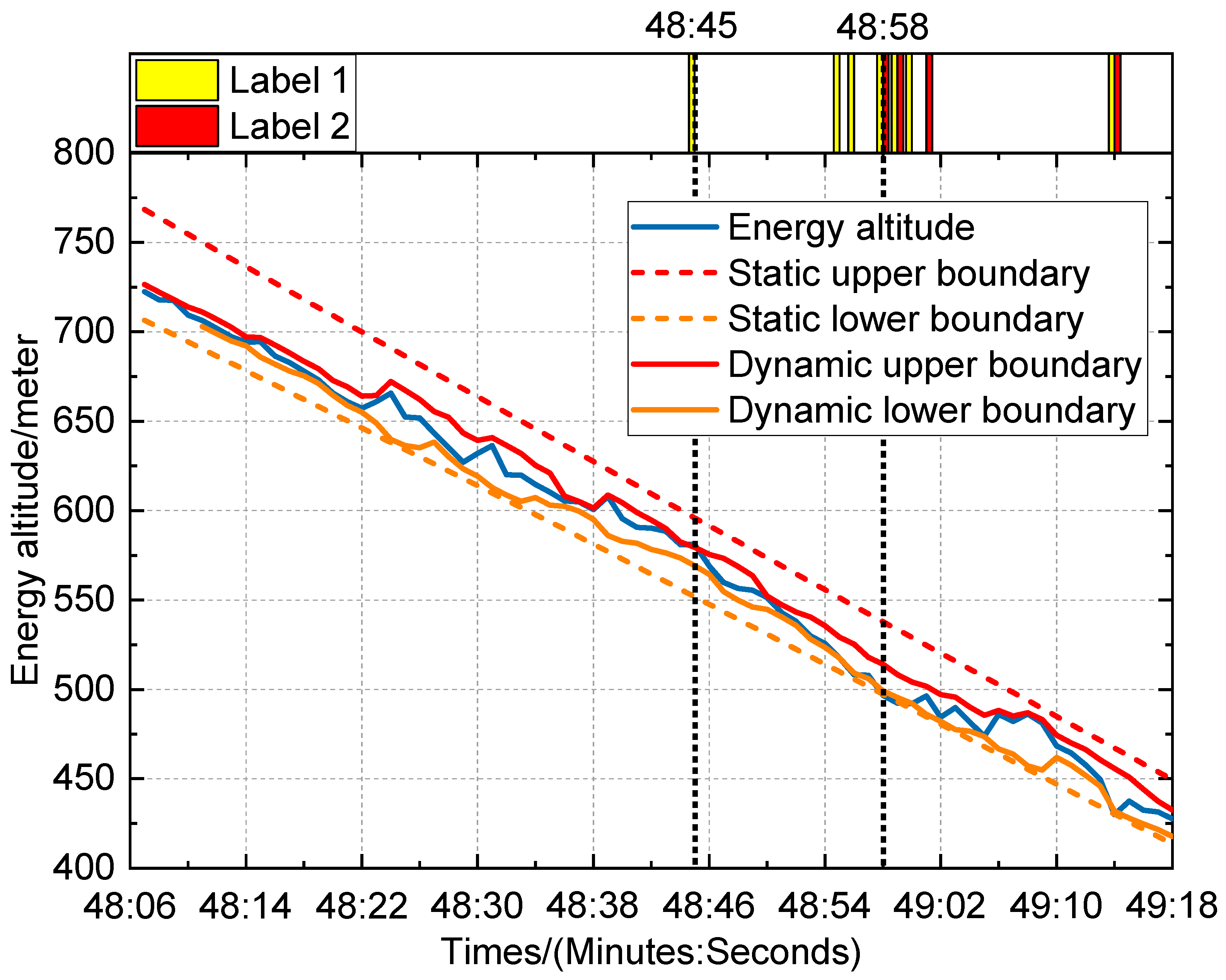
Figure 7 shows the time series visualization results of experimental data under calm-air conditions, which shows the relationship between energy altitude, the dynamic boundary, and the static boundary. In the figure, the blue curve represents the measured energy altitude, the red solid line is the dynamic upper boundary, the orange solid line is the dynamic lower boundary, the red dotted line is the static upper boundary, and the orange dotted line represents the static lower boundary. The yellow column represents the warning state (label 1), and the red column represents the warning state (label 2). The important parameters of the warning event are monitored, as shown in Table 2. It can be seen from the figure that the energy altitude briefly overcomes the dynamic upper boundary at 48:45 (48 min and 45 s), triggering a yellow alert. At 48:58 (48 min and 58 s), the energy altitude is lower than the dynamic lower boundary for 3 s and breaks through the static boundary, triggering a red warning. The visualization results intuitively reflect the evolution process of the energy state from fluctuation to imbalance, providing a key basis for anomaly location.

Figure 7. Timing visualization results and output label positioning under calm wind conditions.

Table 2. The important parameters of the warning events under calm wind conditions.

Times	Correct Airspeed (m/s)	Descent Rate (m/s)	Rotating Speed N1	Energy Altitude (m)	Reason	Label
48:45	78.196	−4.105	56.12	581.07	Higher than the dynamic upper boundary	1
48:55	75.623	−4.389	56.50	517.34	Below the dynamic lower boundary	1
48:56	75.109	−4.308	56.83	508.19	Below the dynamic lower boundary	1
48:58	74.594	−4.145	58.00	496.64	Below the static lower boundary and dynamic lower boundary	1 and 2
48:59	74.594	−4.105	58.62	492.37	Below the static lower boundary and dynamic lower boundary	1 and 2
49:00	75.109	−3.983	59.50	492.04	Below the dynamic lower boundary	1
49:01	76.138	−3.658	60.50	496.31	No anomaly (continuous anomaly in the first three seconds leads to system warning)	2
49:14	74.594	−4.796	52.81	429.89	Below the static lower boundary and dynamic lower boundary	1 and 2

The important parameters of the warning events under calm wind conditions are shown in Table 2. In the verification of the alert state (label 1), at 48 min and 45 s, owing to the influence of turbulence, the energy altitude instantaneously overcomes the dynamic upper boundary, while the early warning system quickly triggers the warning prompt and transmits the energy fluctuation signal to the pilot in time. From 48 min and 55 s to 56 s, the energy altitude is lower than the dynamic lower boundary for 2 s, and the system remains on alert. This design allocates a reasonable operation reaction time for the pilot. Entering the warning state stage (label 2), from 48 min and 58 s to 59 s, the energy altitude falls below the static boundary for 2 s, thus triggering a warning alarm. At 49 min and 1 s, the system issued a warning again. At 48 min and 58 s, the pilot increases the engine thrust from 58% to 60%, which fully verifies the high consistency between the warning logic and the actual operation in the time series. Between 49 min and 2 s and 49 min and 13 s, the energy altitude returns to the dynamic envelope range, and the warning label is automatically reset to 0. However, at 49:14, the energy altitude dropped below both the dynamic lower boundary and the static lower boundary again, triggering Label 1 and Label 2 simultaneously. This indicates that after a brief recovery, the energy state once again became unstable, consistent with the pilot’s further thrust reduction from 60.50% to 52.81% (Table 2). This process verifies that the early warning mechanism can not only accurately respond to abnormal flight conditions but can also return to normal monitoring after the energy state returns to normal, thereby effectively avoiding false positives and omissions, and ensuring the continuous and stable operation of the system.

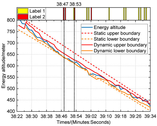
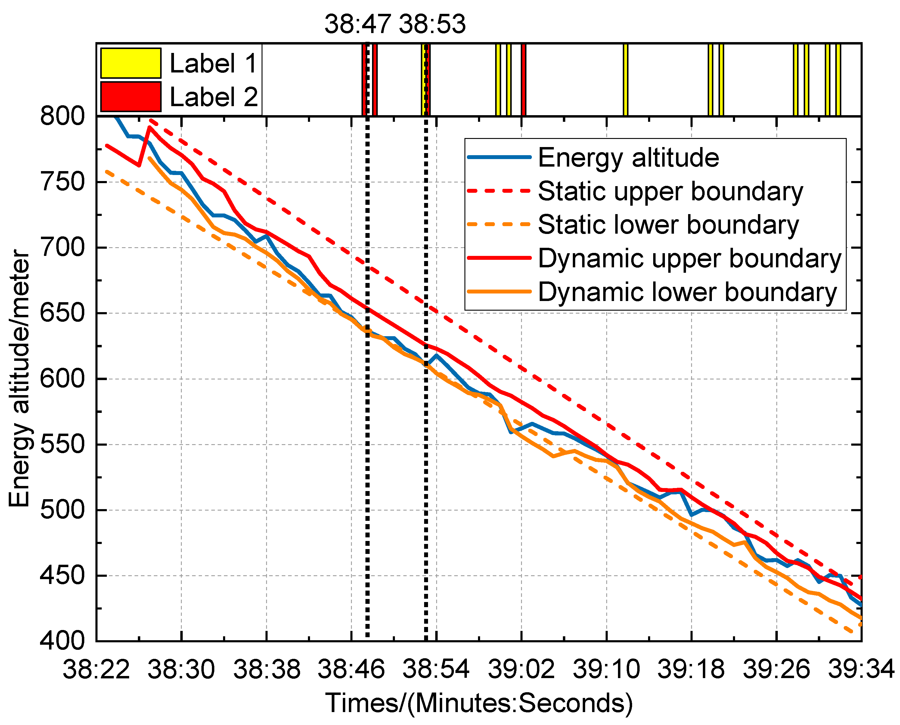
To further verify the feasibility of the mixed boundary method, experimental data under wind-shear conditions are adopted for analysis in this study. The wind-shear parameter corresponds to a 5.14 m/s (10-knot) tailwind shear, meaning the aircraft transitions from a calm-air condition into a 5.14 m/s (10-knot) tailwind field. Figure 8 presents the visualized time-series results of experimental data for the 5.14 m/s (10-knot) tailwind shear case. Key parameters monitored during the warning event are listed in Table 3. It can be seen from the figure that the energy altitude briefly breaks through the static lower boundary at 38 min and 47 s, triggering a red alert. And then at 38 min and 53 s, the energy altitude is below the static lower boundary and dynamic lower boundary.

Figure 8. Timing visualization results and output label positioning under 5.14 m/s tailwind shear.

Table 3. The important parameters of the warning events under 10-knot tailwind shear.

Times	Correct Airspeed (m/s)	Descent Rate (m/s)	Rotating Speed N1	Energy Altitude (m)	Reason	Label
38:47	79.224	−4.227	54.88	646.95	Below the static lower boundary	2
38:48	78.710	−3.942	56.50	638.24	Below the static lower boundary	2
38:53	78.710	−4.308	60.75	618.73	Below the static lower boundary and dynamic lower boundary	1 and 2
39:00	78.710	−4.430	53.38	588.25	Below the dynamic lower boundary	1
39:01	78.196	−4.308	52.63	579.57	Below the dynamic lower boundary	1
39:02	76.138	−4.430	52.06	559.42	Below the static lower boundary	2
39:12	78.196	−4.145	56.19	533.24	Below the dynamic lower boundary	1
39:20	78.196	−4.511	55.69	500.32	Higher than the dynamic upper boundary	1
39:21	78.710	−4.389	55.19	499.86	Higher than the dynamic upper boundary	1
39:28	77.167	−4.227	54.75	457.42	Higher than the dynamic upper boundary	1
39:29	78.196	−4.227	56.38	461.91	Higher than the dynamic upper boundary	1
39:31	77.167	−3.901	56.25	445.23	Higher than the dynamic upper boundary	1
39:32	78.196	−3.942	54.50	450.64	Higher than the dynamic upper boundary	1

The important parameters of the warning events under 5.14 m/s (10-knot) tailwind shear are shown in Table 3. In the verification of the alert state (label 1), the energy altitude fell below the static lower boundary continuously for two seconds between 38 min and 47 s to 48 s, and the early warning system quickly triggers the warning prompt and transmits the energy fluctuation signal to the pilot in time. By 38 min and 53 s, the energy altitude triggered the lower boundary again. It can be observed that the pilot increased the engine speed N1 from 54.88 to 60.75 and maintained the airspeed at 78.71 m/s to adjust the flight state. From 39 min and 0 s to 02 s, the energy altitude stayed below the lower boundary for three consecutive seconds, and the system remained in alert status, providing the pilot with sufficient response time. After 39 min and 20 s, there were three consecutive 2-s breakthroughs in energy altitude beyond the dynamic upper boundary, and the pilots correspondingly increased their airspeed, which once again verified the height consistency between the warning logic and the actual operations in the time series.

3.3.2. Traditional Evaluation Model

To comprehensively verify the advancement and practicability of the hybrid boundary method, we compare it with the traditional single-parameter threshold method and the pure data-driven model lacking physical constraints. Through multidimensional index comparison and scenario verification, we systematically analyze the performance differences of different methods in energy state assessment.

1. Single-parameter threshold method

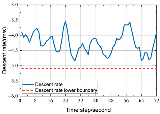
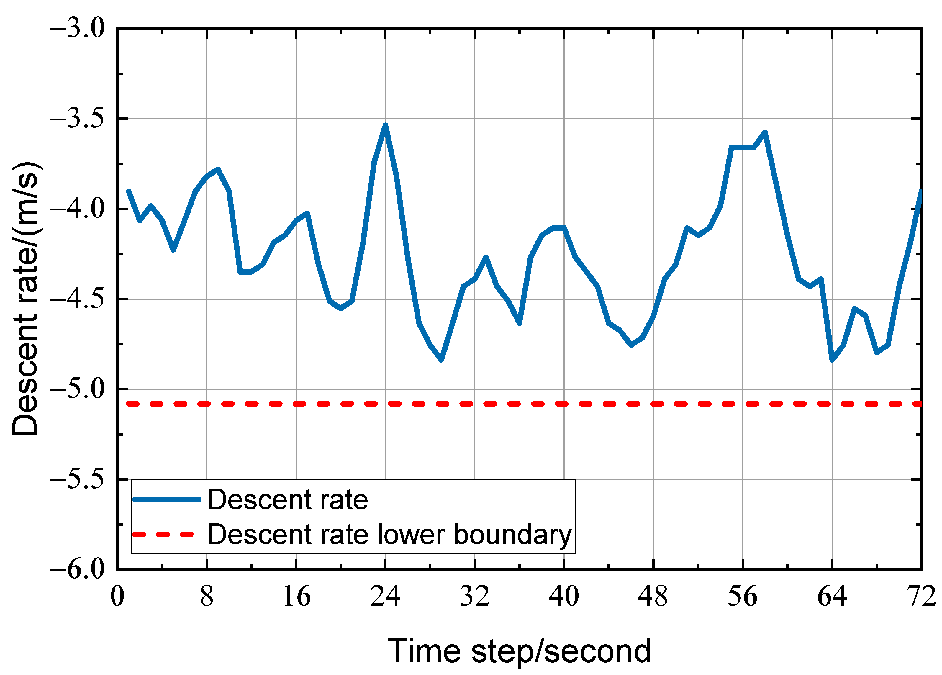
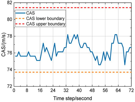
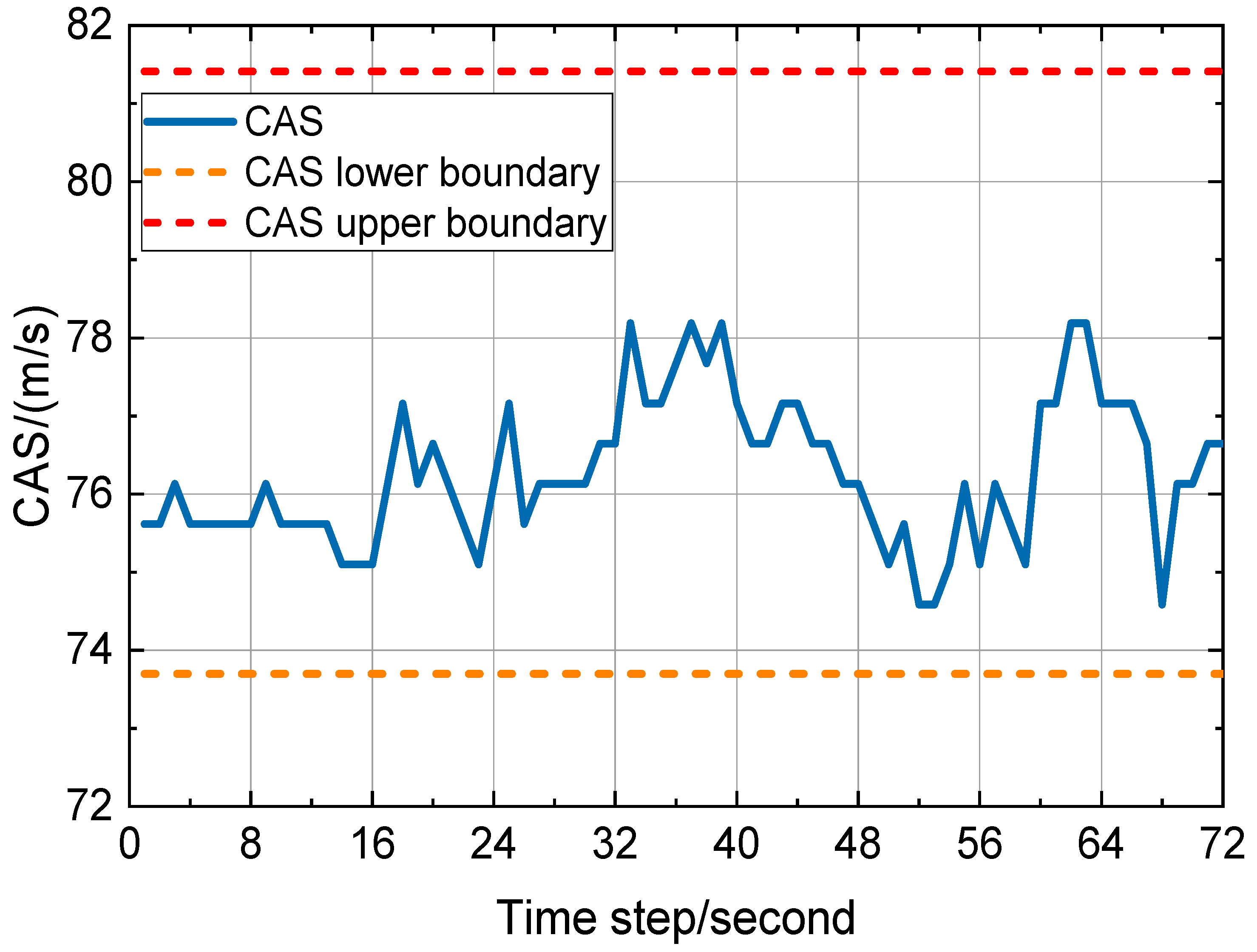
The single-parameter threshold method represents the mainstream method for the evaluation of stable approach in the current civil aviation field, which mainly monitors two independent numerical parameters: speed and descent rate. The experimental data are shown in Figure 9 and Figure 10. The speed of the flight is always stable at 74.59–78.20 m/s (145–152 knots) during the approach process, while the descent rate is maintained at −3.66 m/s (−720 ft/min) through −4.80 m/s (−944 ft/min). Thus, the traditional method determines that this approach is the “stable approach” (label 0).

Figure 9. Decline rate and safety boundary.

Figure 10. Correct airspeed and safety boundary.

As shown in Figure 9 and Figure 10, from 48 min 58 s to 49 min 1 s, traditional parameters indicate that all of the indicators of the aircraft are within the normal range. However, the energy boundary function established in the previous section (Figure 7) clearly shows that the energy altitude continuously overcomes the dynamic lower boundary and static boundary. This contradictory phenomenon reveals the inherent flaws of the traditional single-parameter threshold method: The method only isolates and judges whether one parameter meets the standard, but it cannot identify the potential risks caused by the interaction between parameters. In sharp contrast, the multi-parameter fusion method proposed in this study can more accurately reveal the real state of energy by comprehensively considering the dynamic relationship between energy parameters, thus effectively compensating for the shortcomings of traditional methods.

2. A pure data-driven model without physical constraints

The pure data-driven model trains dynamic boundaries with the aid of Fast Access Recorder (QAR) historical data, which exposes significant limitations owing to the lack of embedded physical constraint mechanisms in flight mechanics. The data-driven visualization results are shown in Figure 11. Compared with Figure 7, the model experiences multiple boundary anomalies during the approach process. For example, at 34 and 52 s, there is an unreasonable contraction of the dynamic boundary, and the dynamic lower boundary is much higher than the energy height trend line. At the same time, the dynamic upper boundary is below the trend line, causing normal fluctuations in flight parameters to be incorrectly marked as abnormal states. At the critical stage of approaching the end 67 s and altitude below 152.4 m (500 feet), the boundary expands abnormally, and the dynamic boundary is lower than the static boundary, which does not meet the strict requirements for energy accuracy in the low-altitude segment. More seriously, compared with Figure 7, the pure data-driven model without physical constraints does not trigger any warning signals during the period of 48 min and 58 s to 49 min and 1 s, which results in significant risk underreporting and fully highlights the negative impact of the lack of physical constraints on the reliability of the model.

Figure 11. Energy altitude and dynamic boundaries (purely data-driven).

Pure data-driven models depend too much on data training and lack physical laws to support them, making it difficult to accurately identify the intrinsic relationship between height and energy changes. This behavior makes it difficult for the dynamic boundaries constructed to meet the requirements of real flight scenarios, ultimately leading to warning failures in complex energy fluctuations, thus highlighting the indispensable role of physical constraints in flight safety assessment.

Therefore, this study innovatively couples the height attenuation function and physical constraints, which theoretically ensures that the boundary function not only conforms to the principles of flight mechanics but can also be dynamically adjusted based on the actual flight altitude. Further, the height decay function gradually tightens the boundary as the height decreases, while the physical constraints frame the scientific boundary of energy changes. The synergistic effect of the two ensures the evaluation system’s rigor.

Traditional static boundaries are limited by a single-parameter evaluation mode, making it hard to fully reflect the flight energy state. Further, pure data models have weak generalization ability in complex scenarios owing to the lack of physical constraints. In contrast, the hybrid boundary method proposed in this study has the following advantages: By integrating multidimensional parameters, it not only breaks through the limitations of single-threshold evaluation but also accurately identifies the energy imbalance hidden behind the data when one parameter meets the standard. Innovatively integrating physical constraints with data-driven technology, the boundary function can achieve smooth dynamic adjustment based on flight altitude and shift according to changing flight environments. At the same time, the warning mechanism based on temporal logic can induce responses in advance during the risk germination stage, allocate sufficient operational time for pilots, and demonstrate stronger environmental adaptability and system stability.

4. Conclusions

The stability assessment of the final approach stage of an aircraft, which is the riskiest stage of the entire flight cycle, is critical for flight safety. The traditional single-parameter threshold monitoring method cannot capture the coupling relationship between kinetic energy and potential energy, or the energy fluctuation characteristics under complex disturbances, making it difficult to meet the needs of modern civil aviation for high-precision and multidimensional stability evaluation. This study focuses on this core issue and systematically conducts research on the stability of the aircraft’s final approach based on energy management. The main tasks completed are as follows:

1. Construct a stability evaluation standard system from the perspective of energy. By defining “energy height” and “balanced energy,” the limitations of traditional “velocity height” dual-parameter independent monitoring are overcome, providing a quantitative basis for multidimensional analysis of energy states;

2. Based on the principles of flight mechanics and civil aviation regulations, a dynamic safety hybrid boundary function is put forth that integrates physical constraints and data-driven approaches. The smooth contraction of boundaries with decreasing height is achieved through a high attenuation mechanism, while the adaptability of boundaries is optimized by using sliding window statistics and a balanced energy triggering mechanism, which improves the issue of the insufficient response of static boundaries to complex disturbances;

3. Comparative tests against traditional threshold models and pure data-driven models demonstrate that the proposed hybrid boundary framework can detect latent energy imbalance risks masked by qualified individual flight parameters, and the time-sequence early warning mechanism can provide sufficient response time for pilots.

The limited number of test samples and narrow coverage of meteorological scenarios restrict the generalizability of the conclusions of this paper. Future research will collect abundant flight data covering multiple aircraft types, wind conditions and altitude ranges to further optimize the generalization performance of the proposed early warning system.

References

- ICAO. Safety Report 2013 Edition; ICAO: Montreal, QC, Canada, 2013. [Google Scholar]
- Yi, B.; Yoo, S.; Jin, Y. Qualitative and Quantitative Risk Assessment of Aircraft System. Aerosp. Eng. Technol. 2006, 5, 223–232. [Google Scholar]
- Bazhenov, G.S. Stability Evaluation of An Airplane with a Digital Multirate Control System In a Lateral Motion. TsAGI Sci. J. 2011, 42, 245–258. [Google Scholar] [CrossRef] [Scilit]
- Asadi, D.; Sabzehparvar, M.; Talebi, H.A. Damaged airplane flight envelope and stability evaluation. Aircr. Eng. Aerosp. Technol. 2013, 85, 186–198. [Google Scholar] [CrossRef] [Scilit]
- Nasir, E.R.; Kuntjoro, W.; Wisnoe, W. Aerodynamic, Stability and Flying Quality Evaluation on a Small Blended Wing-body Aircraft with Canard Foreplanes. Procedia Technol. 2014, 15, 783–791. [Google Scholar] [CrossRef] [Scilit]
- Raghu, V.; Peter, S.; Márk, L.; Vanek, B. Reliability Assessment of Actuator Architectures for Unmanned Aircraft. J. Aircr. 2017, 54, 955–966. [Google Scholar] [CrossRef] [Scilit]
- Jiao, Y.; Sun, H.; Wang, C.; Han, J. Research on Unstable Approach Detection of Civil Aviation Aircraft. Procedia Comput. Sci. 2018, 131, 525–530. [Google Scholar] [CrossRef] [Scilit]
- Hernández-Romero, E.; Valenzuela, A.; Rivas, D. A probabilistic approach to measure aircraft conflict severity considering wind forecast uncertainty. Aerosp. Sci. Technol. 2019, 86, 401–414. [Google Scholar] [CrossRef] [Scilit]
- Du, L. Trajectory tracking sliding mode control for vertical take-off and landing aircraft based on double loop and global Lipschitz stability. PLoS ONE 2025, 20, e0318294. [Google Scholar] [CrossRef] [Scilit] [PubMed]
- Dagal, I.; Erol, B.; Harrison, A.; Mbasso, W.F.; Ibrahim, A.-W. Enhancing Dynamic Control and Stability Assessment of Cessna 172 Aircraft with a PID Controller for New Pilot Trainees. Int. J. Aeronaut. Space Sci. 2025, 26, 2087–2104. [Google Scholar]
- Chu, N.; Ng, K.K.H.; Liu, Y.; Hon, K.K.; Chan, P.W.; Li, J.; Zhang, X. Assessment of approach separation with probabilistic aircraft wake vortex recognition via deep learning. Transp. Res. Part E 2024, 181, 103387. [Google Scholar]
- Lukman, I.E.; Moelyadi, A.M. Longitudinal Static Stability and wake visualization of high altitude long endurance aircraft developed in Bandung institute of technology. J. Phys. Conf. Ser. 2018, 1005, 012050. [Google Scholar] [CrossRef] [Scilit]
- Dong, Z.; Fan, B.; Li, F.; Xu, X.; Sun, H.; Cao, W. TCN-Informer-Based Flight Trajectory Prediction for Aircraft in the Approach Phase. Sustainability 2023, 15, 16344. [Google Scholar]
- Yu, C.; Li, Y.; Zhai, G. Time-frequency attention mechanism-based model for enhancing wind speed prediction accuracy. Expert Syst. Appl. 2025, 265, 126038. [Google Scholar]
- Lush, K.J. A Review of the Problem of Choosing a Climb Technique with Proposals for a New Climb Technique for High Performance Aircraft; R. & M. No. 2557; Aeronautical Research Council, Ministry of Supply: London, UK, 1951. [Google Scholar]
- Lambregts, A.A. Vertical Flight Path and Speed Control Autopilot Design Using Total Energy Principles. In Proceedings of the AIAA Guidance and Control Conference, Gatlinburg, Reston, VA, USA, 15–17 August 1983. AIAA Paper 83-2239. [Google Scholar]
- Faleiro, L.F.; Lambregts, A.A. Analysis and tuning of a ’Total Energy Control System’ control law using eigenstructure assignment. Aerosp. Sci. Technol. 1999, 3, 127–140. [Google Scholar] [CrossRef] [Scilit]
- Zhang, Q.W.; An, J.W. A New Method for Designing Decoupling Controller of Flight Speed/Flight Path Based on Total Energy Control. Chin. J. Aeronaut. 2004, 25, 389–392. (In Chinese) [Google Scholar] [CrossRef]
Disclaimer/Publisher’s Note: The statements, opinions and data contained in all publications are solely those of the individual author(s) and contributor(s) and not of MDPI and/or the editor(s). MDPI and/or the editor(s) disclaim responsibility for any injury to people or property resulting from any ideas, methods, instructions or products referred to in the content. |
© 2026 by the authors. Licensee MDPI, Basel, Switzerland. This article is an open access article distributed under the terms and conditions of the Creative Commons Attribution (CC BY) license.