Flight Dynamics of a Hover-Capable Air-Launched Unmanned Aerial Vehicle ^†

Abstract

This paper discusses the development of a fully nonlinear flight dynamics model of a hover-capable Air-Launched Uncrewed Aerial System (ALUAS) in order to (1) understand the dynamics, controllability, and airloads during complicated maneuvers and (2) gain insights from simulation to inform the design and operation of future ALUASs. Prior studies conducted wind tunnel tests on full-scale models to measure the airloads on the propeller, isolated fuselage, and full aircraft. The flight dynamics model, once corrected with the test data, was used to simulate maneuvers including hover-to-cruise transition, cruise-to-hover transition, ground launch, air launch from a moving helicopter, and air launch with asymmetric wing unfolding. These simulations demonstrate the capability of the vehicle to perform complicated maneuvers to meet various mission objectives in challenging environments.

1. Introduction

Air-launched Uncrewed Aerial Systems (ALUASs) are an emerging class of highly versatile air vehicles that can satisfy a broad range of desired mission requirements for civilian and military applications, including reconnaissance, search and rescue, emergency response, surveying and mapping, and military engagement. The defining characteristic of an ALUAS is the capability to be launched as a projectile, increasing the aircraft’s range and usability in infrastructure-less environments and decreasing the time to altitude. Deployment strategies of particular interest include tube launching from ground to air and launching from a flying aircraft (air to air). Indeed, this new class of aircraft provides a solution to the lowered range and speed commonly faced by UASs that rely on electric powertrains. However, launching in this manner imposes a stowability constraint on the design of ALUASs as all parts of the system must fit inside a tube; contrarily, realizing the potential range benefits of ALUASs compels the use of high-aspect-ratio wings and low-disk-loading rotors. These conflicting requirements necessitate the use of morphing structures on the aircraft. Morphing can be achieved using a series of mechanisms which have the ability to fold the ALUAS’ rotors, wings, and stabilizers, allowing the aircraft to fit inside of a launcher. Upon being launched from the tube, said mechanisms can then unfold the ALUAS’ lifting and thrusting systems to enter into either a horizontal or vertical flight condition. Moreover, hover capability is critical for ALUASs to be recoverable in environments as complex as those which they can be launched from, as well as for them to navigate and perform complicated missions in dense urban environments. Hence, there is significant interest in developing ALUASs that are capable of efficient hover without compromising the high lift-to-drag ratio in cruise.

Once launched from the tube, ALUASs go through various transient flight phases, complex maneuvers, and rotor/wing deployments to accomplish their mission. Therefore, it is important for these systems to be stable during all these maneuvers and for the transitions to be made in a seamless fashion. A particularly challenging maneuver is air launch from a mothership. Passing through the wake of the mothership adversely influences the dynamics of the small UAS for a period of time even after it has gotten out of the wake. If the mothership is cruising at high speeds, not only will the ALUAS experience a component of downwash, but it will see an abrupt, large increase in airspeed. This leads to an increase in aerodynamic force proportional to $V_{\infty }^2$ and can severely alter the dynamics of the aircraft, especially if the ALUAS is equipped with large lifting surfaces. More specifically, the effect of the increased airflow on the ALUAS could lead to large changes in the angle of attack or sideslip, which largely depends on the angle of launch relative to the mothership.

To ensure that ALUASs can perform various missions and remain stable throughout all maneuvers, flight control laws must be developed and validated through flight testing. This is a difficult challenge, especially for air launch maneuvers, due to the limited number of ALUAS prototypes presently available to generate flight test data. Yang et al. [1] documented many challenges after the flight testing of tube-launched prototypes in terms of launch uncertainties as well as control design. A control system for ALUASs needs to ensure that nominal air launch maneuvers can be performed and at the same time be able to reject external disturbances such as wind gusts and rotor wakes. Control systems on simpler aircraft that perform relatively straightforward maneuvers in rather benign environments, such as a conventional quadrotor UAS, can be tuned experimentally through a combination of indoor and outdoor flight testing with little consequence. This is in contrast to an air launch scenario, where experimental tuning of the controller via flight testing is complicated by the broad range of flight conditions and transient maneuvers, including projectile motion, transitions between different flight modes, and unfolding of the rotors and wings. Denton et al. [2] approached this problem by utilizing a wind tunnel to experimentally tune the controller before attempting a tube launch of their prototype.

All of this adds to the motivation for developing a high-fidelity flight dynamics model of an ALUAS. With a model, novel control strategies can be explored and applied to the real aircraft with higher confidence. In addition, a flight dynamics model enables states and airloads of ALUASs to be investigated and design principles to be formulated from simulation and fed back into the design of the next generation of ALUAS prototypes.

ALUASs have previously been studied both experimentally and theoretically and can be classified as either fixed-wing or rotary-wing aircraft. Under the fixed-wing category, Aerovironment’s Switchblade [3] is capable of being launched from a tube, quickly deploying its wings and stabilizers to enter into a horizontal flight configuration. Another development under the fixed-wing category came from Anduril Industries, who developed the ALTIUS-M platform [4]. These tube-launched loitering munitions can be deployed from the ground or air to accomplish a wide range of missions. The rotary-wing category includes the Streamlined Quick-Unfolding Investigation Drone (SQUID) developed by Bouman et al. [5], which is designed to be ballistically launched. Furthermore, this category includes a tube-launched jettisonable-fin foldable multirotor [6], and also a gun-launched micro air vehicle (GLMAV) which was previously developed and flight-tested by Denton et al. at Texas A&M University [2]. An air-launched Tailsitter UAS capable of operating in both vertical and horizontal flight was also previously designed and flight-tested by Cai et al. [7] and Dooher et al. [8]. This aircraft has coaxial propellers and uses a thrust vector mechanism to control roll and pitch attitude in hover. It has foldable wings to enable the aircraft to be stowed in a tube for launch, and can fold/unfold them using servo actuators. Other works include conceptual studies [9,10], with a few recent studies detailing cruising flight tests of foldable prototypes [11].

This work aims to develop a flight dynamics model of a Tailsitter ALUAS prototype that was developed at Texas A&M University. This aircraft was selected because all details of the vehicle design were available. In addition, experimental data from a wind tunnel test of the aircraft was available for validating and refining the propeller and airframe aerodynamic models. Previously, flight dynamics models have been developed for tube-launched aircraft. For example, a catapult-launched tandem variable sweep UAV was developed by Gao et al. [12]. Cheng et al. [13] developed a flight dynamics model for a tube-launched tandem-winged UAV to perform stability analysis in the transition region where the aircraft unfolds its wings. Yang et al. developed a six-degree-of-freedom dynamics model of a rocket-propelled foldable UAV [1]. Air-launched folding-wing UAVs launched from a high-altitude balloon have also been studied by Zhang et al. [14].

Tailsitter modeling has been previously studied; for example, a quadrotor biplane tailsitter (QBiT) was modeled by Saetti et al. [15] using a CFD simulation. In addition, Gadag et al. [16] utilized blade element theory and lifting-line theory to model the flight dynamics of a QBiT. Despite lower-order modeling, the flight dynamics predictions matched well against measured flight data. The Tailsitter ALUAS that is studied in this work has coaxial propellers, which have previously been modeled using dynamic inflow [17] and free wake [18]. Furthermore, as the Tailsitter ALUAS has both rotary wings and fixed wings, rotor–wing interactions become relevant, and have been previously modeled using CFD [19]. As the present air-launched Tailsitter can fold and unfold (morph) its wings, the dynamics of morphing aircraft become relevant. Morphing aircraft have been previously examined by Elliot et al. [20], Gao et al. [12], Cheng et al. [13], Yang et al. [1], Ryseck et al. [21], and Zhang et al. [14]. Finally, to ensure the Tailsitter can perform an air launch as well as transition between hover and cruise, control systems must be designed. Zhang et al. [14] explored the control and trajectory optimization of drones that are air launched from hot air balloons, while Saetti et al. [15] explored novel dynamic inversion control for autonomous hover-to-cruise transition.

While many experimental and computational studies have been performed on the topic of tube-launched aircraft, many of them have been limited to either fixed-wing aircraft or rotary-winged aircraft. The present study contributes by presenting nonlinear flight dynamics modeling and analysis of a coaxial Air-Launched UAS that is also capable of transition between hover and cruise. The paper starts with an overview of the Tailsitter ALUAS, followed by flight dynamics modeling, and the hover test methodology. A validation of propeller aerodynamic models using hover test data is then presented, succeeded by the results and discussion of complex ALUAS maneuver simulations, including a transition maneuver from hover to horizontal flight (cruise), a ground launch, and finally an air launch with symmetric and asymmetric wing deployment.

2. Tailsitter ALUAS Design

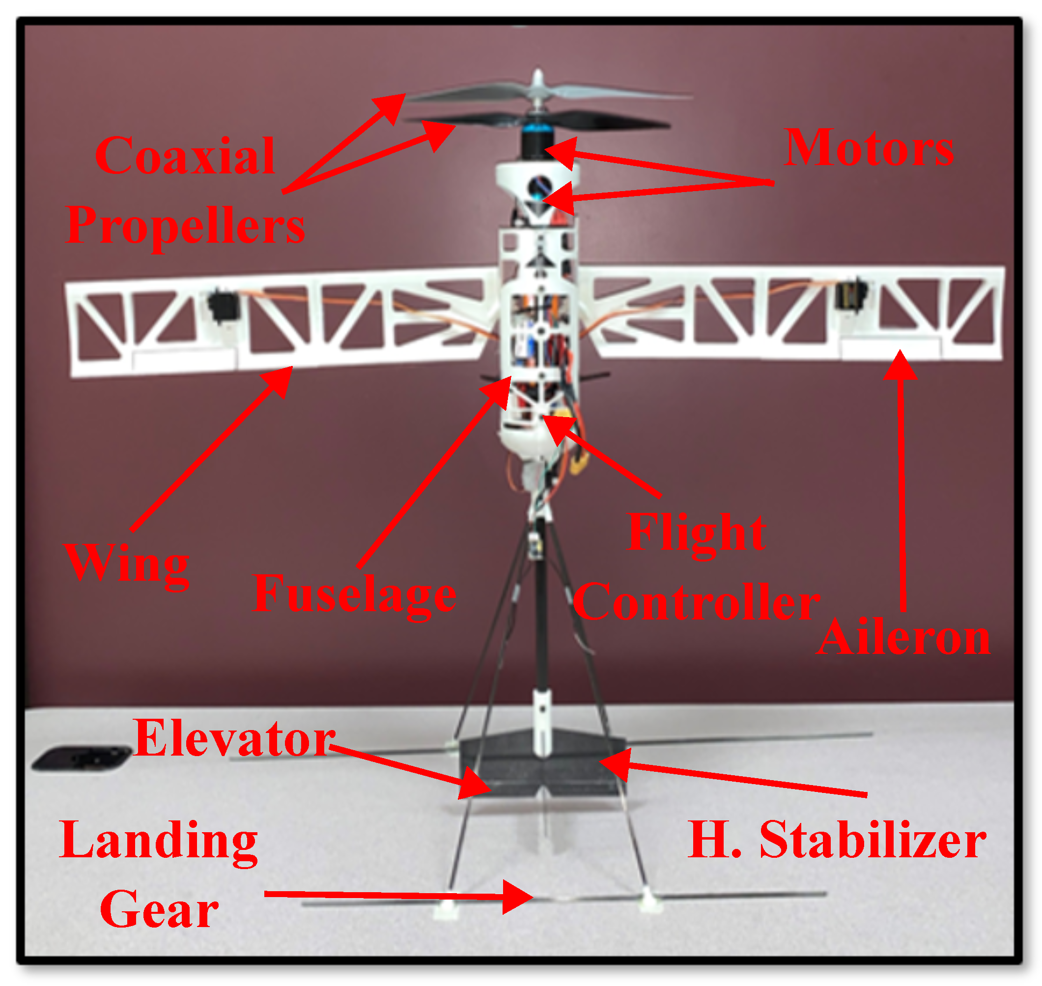
The realized Tailsitter UAS is shown in Figure 1, where some of the major components are labeled.

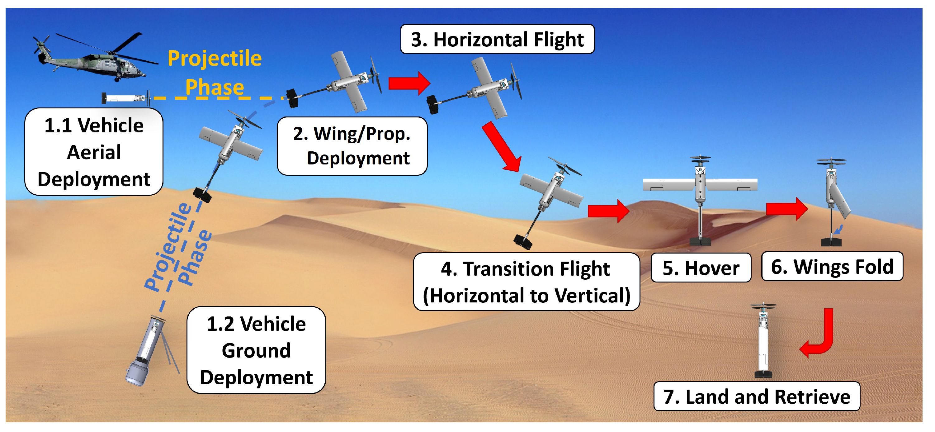
The main feature of the Tailsitter ALUAS is its ability to be air launched from a moving vehicle and then enter a particular flight condition. The Tailsitter can operate in both vertical and horizontal flight conditions, which combines the high maneuverability of a hover-capable UAS with the efficiency of forward-flying fixed-wing aircraft, enabling the vehicle to perform a wider range of missions. A summary of the nominal operation of the Tailsitter is shown in Figure 2. This vehicle is designed to be launched from a tube, whether from an air launch (1.1) or a ground launch station (1.2), which requires the vehicle to be able to fold its wings to fit compactly inside. After launch, the vehicle enters into a projectile phase, where, at a certain point, the wings and propellers are deployed (2) to begin horizontal flight (3). From this flight configuration, the vehicle can transition (4) back to a vertical flight configuration (5) and eventually fold its wings (6) to land and be retrieved (7).

The main characteristics of the vehicle are highlighted in

Table 1. Tailsitter ALUAS characteristics.

Characteristic	Imperial	SI
Propeller Radius	0.45 ft	0.14 m
Main Wing Span	2.62 ft	0.8 m
Stabilizer Span	0.5 ft	0.14 m
Length	2 ft	0.619 m
Fuselage Diameter	0.23 ft	0.07 m
Weight	2.2 lb	1 kg
Cruise Speed	66 fps	20 m/s

. It uses two electric motors for propulsion, as well as two 11 × 7 propellers in a coaxial configuration. Further information about the design and development of the Tailsitter is given by Cai et al. [7] and Dooher et al. [8], as well as by Stewart et al. [22]. A video demonstrating the capability of the Tailsitter can be found at [23].

3. Methodology

3.1. Flight Dynamics Model

In order to better understand the dynamic states and airloads of an ALUAS and gain insights that could inform the design and operation of future ALUASs, a flight dynamics model is developed. This is accomplished using the Rotorcraft Comprehensive Analysis System v22.08.u20a (RCAS) developed by Advanced Rotorcraft Technology (ART), (Fremont, CA, USA) [24]. In general, the RCAS can be used for structural, aerodynamic, and flight dynamics analysis of an arbitrary vehicle at any scale. Structural modeling in the RCAS can be rigid or elastic. A vehicle’s structure can be represented by a series of primitive elements such as beams, springs, hinges, etc., which allows complicated multi-body dynamic models to be defined. Aerodynamic modeling in the RCAS uses lifting-line and blade element approaches for calculating airloads produced by wings and rotors, respectively. Induced velocity models within the RCAS range from simple uniform inflow models to higher-fidelity models such as free wake models. Furthermore, the RCAS can be coupled with external codes such as Python or CFD for additional fidelity. After defining structural and aerodynamic models for a given vehicle, coupled aerodynamic and structural analysis can be performed. This includes trimmed analysis and nonlinear six-degree-of-freedom (6-DOF) flight dynamics analysis.

The flight dynamics model of the Tailsitter in the RCAS has six degrees of freedom and the structural components are modeled as rigid. To assist in the analysis of the Tailsitter’s motion, coordinate system definitions are made: Let

$\mathcal{N}=\{\mathcal{O},{\widehat{\mathbf{n}}}_1,{\widehat{\mathbf{n}}}_2,{\widehat{\mathbf{n}}}_3\}$ be a right-handed inertial coordinate system centered about an arbitrary point $\mathcal{O}$, where ${\widehat{\mathbf{n}}}_i$ are mutually orthogonal unit vectors $\forall i\in \{1,2,3\}$. Similarly, let $\mathcal{B}=\{b,{\widehat{\mathbf{b}}}_1,{\widehat{\mathbf{b}}}_2,{\widehat{\mathbf{b}}}_3\}$ be a rotating coordinate system attached to the body and centered about the center of mass b. The passive transformation from the inertial coordinate system to the body coordinate system is given by Equation (1):

$$T_{\mathcal{N}}^{\mathcal{B}}=T_2\left(\theta \right)T_1\left(\varphi \right)T_3\left(\psi \right)$$

(1)

This transformation uses a 3-1-2 Euler angle sequence ($\psi -\varphi -\theta$), which was chosen to avoid a singularity at a pitch angle ($\theta$) of +/$-90°$ as the nominal operation of the vehicle involves both vertical and horizontal flight. In this case, although the roll angle $\varphi$ is singular at +/$-90°$, the vehicle is assumed to not operate at such extreme orientations. The Euler angle rates can be found from the angular velocities expressed in the body coordinate system using the transformation given by Equation (2):

$$\left\{\begin{array}{c}\dot{\varphi }\\ \dot{\theta }\\ \dot{\psi }\end{array}\right\}={\displaystyle \frac{1}{cos\left(\varphi \right)}}\left[\begin{array}{ccc}cos\left(\theta \right)cos\left(\varphi \right)& 0& sin\left(\theta \right)cos\left(\varphi \right)\\ sin\left(\varphi \right)sin\left(\theta \right)& cos\left(\varphi \right)& -cos\left(\theta \right)sin\left(\varphi \right)\\ -sin\left(\theta \right)& 0& cos\left(\theta \right)\end{array}\right]\left\{\begin{array}{c}p\\ q\\ r\end{array}\right\}$$

(2)

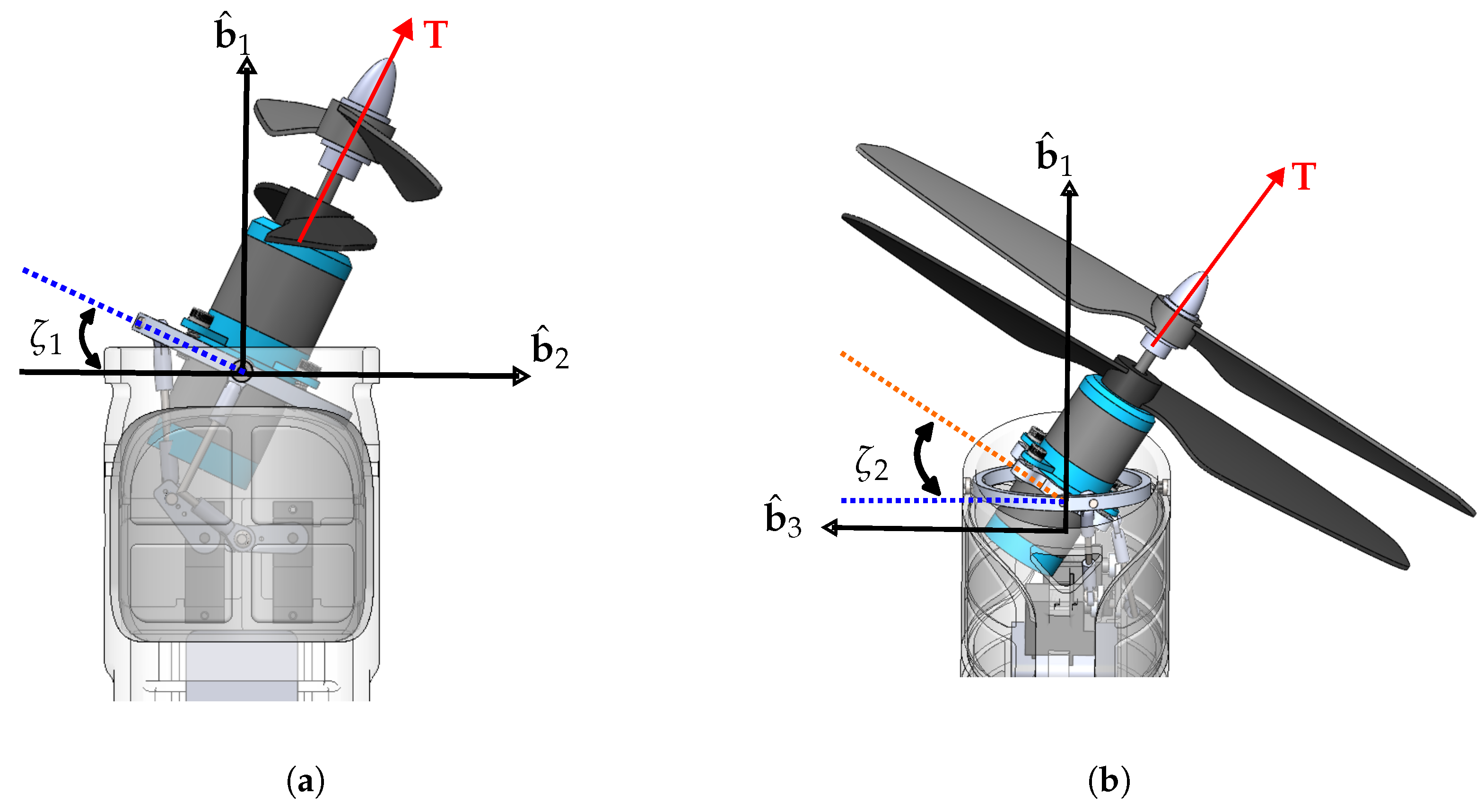
The orientation of the thrust vector at an instant of time can be described by angles ${\zeta }_1$ and ${\zeta }_2$: ${\zeta }_1$ is the angle between the outer gimbal ring and the body coordinate system, and ${\zeta }_2$ is the angle between the outer gimbal ring and the inner gimbal ring. Figure 3 shows first a positive deflection of the outer gimbal (denoted with blue dashes) with deflection angle ${\zeta }_1$ in Figure 3a followed by a positive deflection of the inner gimbal (denoted with orange dashes) with deflection angle ${\zeta }_2$ in Figure 3b.

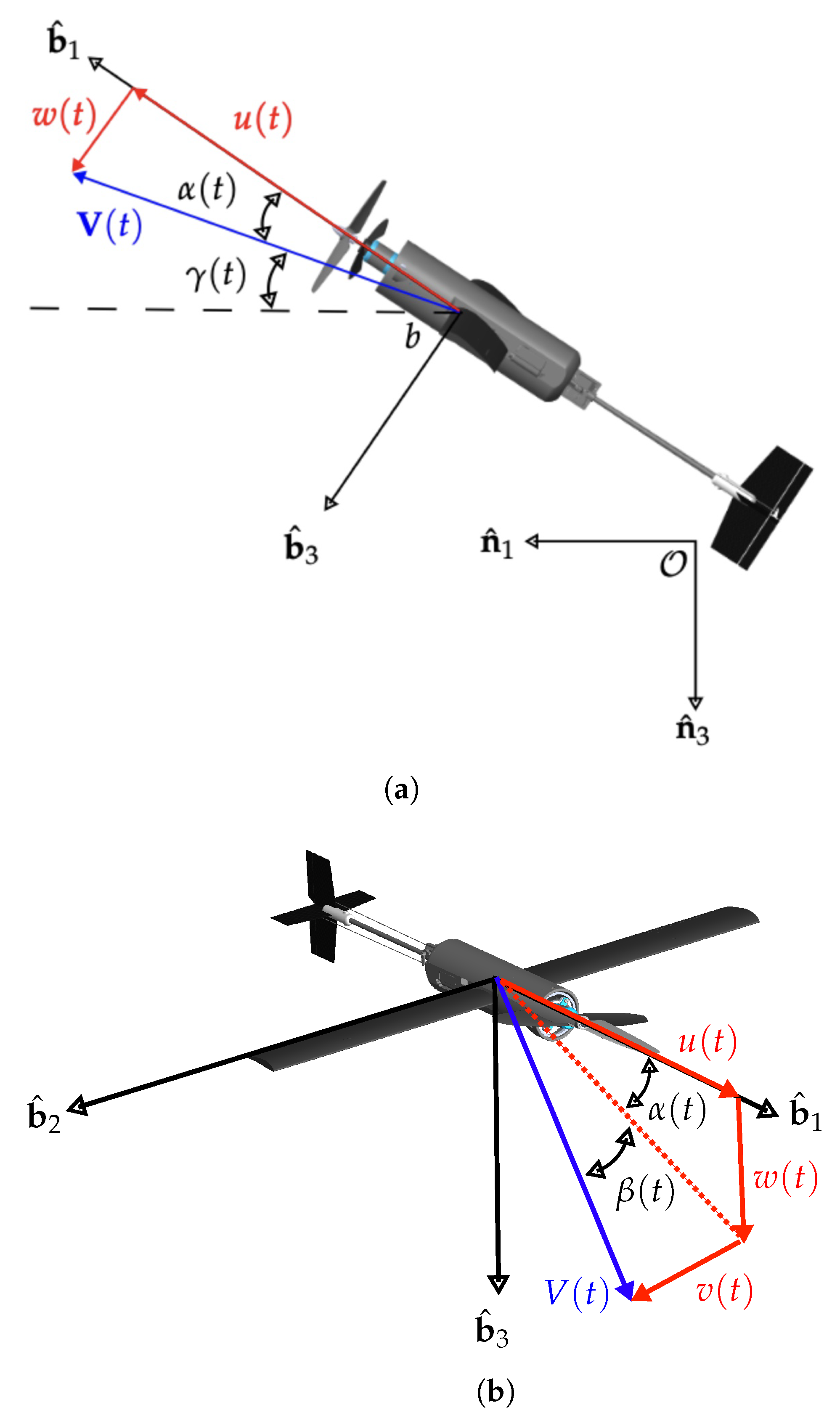
The position of the vehicle at any instant in time is given by the vector $\mathbf{r}\left(t\right)=x\left(t\right){\widehat{\mathbf{n}}}_1+y\left(t\right){\widehat{\mathbf{n}}}_2+z\left(t\right){\widehat{\mathbf{n}}}_3$ expressed in the inertial coordinate system. The aircraft’s velocity, given by $\mathbf{V}\left(t\right)=u\left(t\right){\widehat{\mathbf{b}}}_1+v\left(t\right){\widehat{\mathbf{b}}}_2+w\left(t\right){\widehat{\mathbf{b}}}_3$ and expressed in the body coordinate system, is used to calculate aerodynamic angles. The aerodynamic angles that are responsible for the aerodynamic loading on the aircraft are the angle of attack ($\alpha$) and the angle of sideslip ($\beta$), which are responsible for the longitudinal and lateral aerodynamic forces and moments, respectively. The trajectory of the aircraft can be quantified by the flight path angle ($\gamma$). These three angles are defined in Equation (3):

$$\left\{\begin{array}{c}\alpha \\ \beta \\ \gamma \end{array}\right\}=arctan\left\{\begin{array}{c}w/u\\ v/u\\ {\displaystyle \frac{-\dot{z}}{\sqrt{{\dot{x}}^2+{\dot{y}}^2}}}\end{array}\right\}$$

(3)

The angles of attack and sideslip are both functions of u, v, and w, which are the inertial velocities of the vehicle expressed in the body coordinate system. However, the flight path angle is a function of $\dot{x}$, $\dot{y}$, and $\dot{z}$, which are the inertial velocities of the vehicle expressed in the inertial coordinate system. These angles of interest are shown in Figure 4, where Figure 4a shows the three-degree-of-freedom case (longitudinal), and Figure 4b shows the general six-degree-of-freedom case (both longitudinal and lateral).

The state vector of interest is given as ${[x,y,z,u,v,w,\varphi ,\theta ,\psi ,\dot{\varphi },\dot{\theta },\dot{\psi },\alpha ,\beta ,\gamma ]}^T$, where all variables are functions of time. The associated time-varying control vector is defined as ${[{\delta }_{{\zeta }_1},{\delta }_{{\zeta }_2},{\delta }_{{\Omega }_{diff}},{\delta }_{{\Omega }_T},{\delta }_a,{\delta }_e,{\delta }_r]}^T$, where ${\delta }_{{\zeta }_1}$ is the roll gimbal angle, ${\delta }_{{\zeta }_2}$ is the pitch gimbal angle, ${\delta }_{{\Omega }_{diff}}$ is the propeller differential speed command, ${\delta }_{{\Omega }_T}$ is the throttle command for both upper and lower propellers, ${\delta }_a$ is the aileron deflection command, ${\delta }_e$ is the elevator deflection command, and ${\delta }_r$ is the rudder deflection command.

The following subsections will provide a description of the structural and aerodynamic components of the Tailsitter starting with definitions of mass and inertia properties, implementation of the coaxial propellers and associated thrust-vectoring mechanism, aerodynamic modeling of the main wing and stabilizers, definition of the wing-folding mechanism, aerodynamic modeling of the fuselage, and, finally, the definition of the helicopter mothership used to air launch the Tailsitter. Finally, the design of control systems which enable the Tailsitter to perform its various maneuvers is discussed.

3.1.1. Mass and Inertia Properties

The mass of the vehicle is approximately 1 kg. The approximate rotational inertia tensor is taken from the computer-aided design (CAD) model of the Tailsitter. In general, the time-varying composite inertia tensor about the mass center of the vehicle, b, is expressed in the body coordinate system in Equation (4) (assuming two planes of symmetry):

$${\left[I_b\right]}^{\mathcal{B}}=\left[\begin{array}{ccc}{I}_1\left(t\right)& 0& 0\\ 0& I_2\left(t\right)& 0\\ 0& 0& I_3\left(t\right)\end{array}\right]$$

(4)

The inertia tensor includes contributions from the gimbal mechanism, wings, and fuselage, where both the center of mass location and the inertia tensor of the entire vehicle change due to the unfolding/folding of the wings and deflection of the gimbal mechanism. These effects are modeled in the RCAS under the following assumptions:

1.

The composite inertia tensor about the center of mass will only change with the unfolding or folding of the wings.

2.

The inertia contribution from the gimbal system is taken when the gimbal is un-deflected and grouped with the fuselage inertia tensor.

3.

The center of mass location will not change for all cases.

This leaves the fuselage, right wing, and left wing to all have their own separate inertia values, which form the composite inertia tensor about the center of mass.

3.1.2. Coaxial Propellers

The propellers are both modeled in the RCAS as identical rigid counter-rotating two-bladed propellers with similar geometry to those on the realized vehicle. The propeller diameter is approximately 11 inches and has twist and taper. Propeller thrust and torque are computed in the RCAS using a blade element method, which requires knowledge of the sectional lift, drag, and pitching moment coefficients, $C_l$, $C_d$, and $C_m$, respectively. The airfoil for each blade is a Clark-Y. The airfoil aerodynamics are generated as a function of the angle of attack and Reynolds number using XFOIL [25]. XFOIL is a piece of software used for aerodynamic analysis of airfoils and is capable of accounting for the physics seen at the low Reynolds numbers [26] where the Tailsitter operates. XFOIL can easily be run through another piece of software named XFLR5 (v6.61) [27], which introduces a graphical user interface (GUI). The chosen induced velocity model has uniform inflow where $\lambda =const.$ and does not vary with radial or azimuthul location. Upper-to-lower-propeller interference is considered, and the mean interference velocity is determined by (1) the induced velocity of the upper propeller, and (2) the separation distance between propellers, which is further detailed by Saberi et al. [28,29]. The thrust and torque of the lower propeller are then computed and subsequently added to that of the upper propeller.

Each propeller’s angular velocity can be independently changed, allowing for a non-zero torque about the propeller axis which can be leveraged to control the yaw angle of the aircraft. This concept will commonly be referred to throughout this work as ‘differential RPM control’.

3.1.3. Thrust-Vectoring Mechanism

The direction of total thrust is along the axis of the propellers. This thrust vector can be modified by changing either the roll or the pitch of the gimbal. On the realized vehicle, the outer gimbal ring controls the roll of the thrust vector. The inner gimbal ring, which is attached to the outer gimbal, is used to control the pitch of the thrust vector relative to the outer gimbal.

This mechanism is replicated within the RCAS by using two controlled hinges for roll and pitch, defined by angles ${\zeta }_1$ and ${\zeta }_2$, respectively, as shown in Figure 3. ${\zeta }_1$ is the angle between the outer gimbal ring and the body coordinate system, and ${\zeta }_2$ is the angle between the outer gimbal ring and the inner gimbal ring. Depending on these angles, provided as control input, the thrust vector generates a moment about the center of mass of the Tailsitter, causing rotational motion about an arbitrary axis which can be leveraged to control the attitude of the aircraft. The roll and pitch thrust vector angles are limited to +/−30° as they are on the realized platform.

3.1.4. Fixed-Wing Lifting Surfaces

The fixed-wing lifting surfaces on the Tailsitter include the main wing, which is rectangular, and the horizontal and vertical stabilizers, which are tapered. All three surfaces have a zero incidence angle relative to the fuselage. The lift, drag, and pitching moment for these lifting surfaces are computed in the RCAS using lifting-line theory, which requires knowledge of sectional lift, drag, and pitching moment coefficients, similar to the blade element method mentioned previously. At all spanwise sections of the main wing, the airfoil is a Selig 1223, whose lift, drag, and pitching moment coefficients are entered into the RCAS through a lookup table generated by XFOIL. The lookup table is a function of both the angle of attack and the Reynolds number. The airloads for the finite-spanned wing are calculated under a uniform downwash assumption. The horizontal and vertical stabilizers of the vehicle are modeled as flat plates, where their sectional two-dimensional aerodynamic coefficients are approximated by linear relationships. The lift coefficient is defined by $C_l=2\pi {\alpha }_e$, where ${\alpha }_e$ is the sectional effective angle of attack. The drag coefficient is approximated by $C_d=C_{do}=const.$ and the pitching moment ($C_m$) is zero. Airloads for each finite-spanned stabilizer are calculated in the same way as the wing with uniform downwash.

To increase the fidelity of the fixed-wing aerodynamic model, empirical corrections are made using available wind tunnel data from the full aircraft (wings, fuselage, and stabilizer). These corrections are used in the form of a constant bias that is added to each of the 3-D airloads ($C_L$, $C_D$, $C_M$) computed by lifting-line theory. The wind tunnel used for these experiments is a closed-loop low-speed tunnel with a 4 foot by 3 foot (1.2 m by 0.9 m) test section. More information about this setup can be found in [22].

The aileron control surfaces are modeled by first generating two-dimensional airfoil polars for the lift, drag, and pitching moment as a function of the angle of attack, Reynolds number, and deflection angles using XFOIL. The spanwise locations along the wing where the ailerons lie then rely on the RCAS to interpolate between the deflection angle, Reynolds number, and angle of attack to determine the sectional lift, drag, and pitching moment coefficients. Finally, the loads from the aileron sections are integrated along with the other non-aileron sections of the wing using lifting-line theory. The ailerons are limited to control surface deflections, ${\delta }_a\in [-20°,20°]$.

The elevator control surface is taken as a percentage chord of the horizontal stabilizer. The change in pitching moment with respect to elevator deflection, outlined by Nelson [30], is defined by Equation (5):

$${\displaystyle \frac{\partial C_M}{\partial {\delta }_e}}=-V_h\eta C_{L_h\alpha }\tau$$

(5)

where $V_h$ is defined as the horizontal tail volume coefficient, $C_{L_h\alpha }$ is the lift curve slope of the horizontal stabilizer, $\tau$ is the flap effectiveness parameter, and $\eta$ is the tail efficiency. The dimensionalized contribution to the pitching moment about the center of mass due to the elevator deflection can be determined using the linear relationship shown in Equation (6):

$$M\left({\delta }_e\right)=QSc{\displaystyle \frac{\partial C_M}{\partial {\delta }_e}}{\delta }_e$$

(6)

This moment contribution is added to the existing pitching moment contribution to obtain the total pitching moment about the center of mass, $M_{cg}=M\left(\alpha \right)+M\left({\delta }_e\right)$, where the elevator deflection angle is limited to ${\delta }_e\in [-25,25]$. Following the sign convention outlined by Nelson, a negative elevator angle indicates that the elevator trailing edge is pointing upward; hence, the associated pitching moment caused by elevator deflection is positive about the ${\widehat{\mathbf{b}}}_2$ axis.

Because the vertical stabilizer geometry is identical to the horizontal stabilizer, the rudder control surface is modeled in an identical way to the elevator. The difference is that now the rudder contributes an additive yawing moment about the center of mass. A negative rudder deflection, ${\delta }_r$, will produce a positive yawing moment, indicating that, for a negative rudder deflection, the trailing edge points to the starboard side of the aircraft body. The rudder is limited to ${\delta }_r\in [-25,25]$.

3.1.5. Wing-Folding Mechanism

In order to perform ground and air launch missions, the main wing of the Tailsitter must be folded in order to fit inside a launcher. Subsequently, after launch, the wing must be unfolded for the Tailsitter to fly. The folding method used to overcome this challenge was inspired by how birds fold their wings (rotating them down and backward until they are tucked in and almost flush with the rest of their body). To implement this on the realized aircraft, each half of the main wing is mounted to the fuselage along oblique axes, and two linear actuators are used to provide torque to rotate each wing. Linear actuators, as opposed to traditional servo motors, are chosen to drive the actuation as their shape can more easily fit into the fuselage while being large enough to provide the necessary torque.

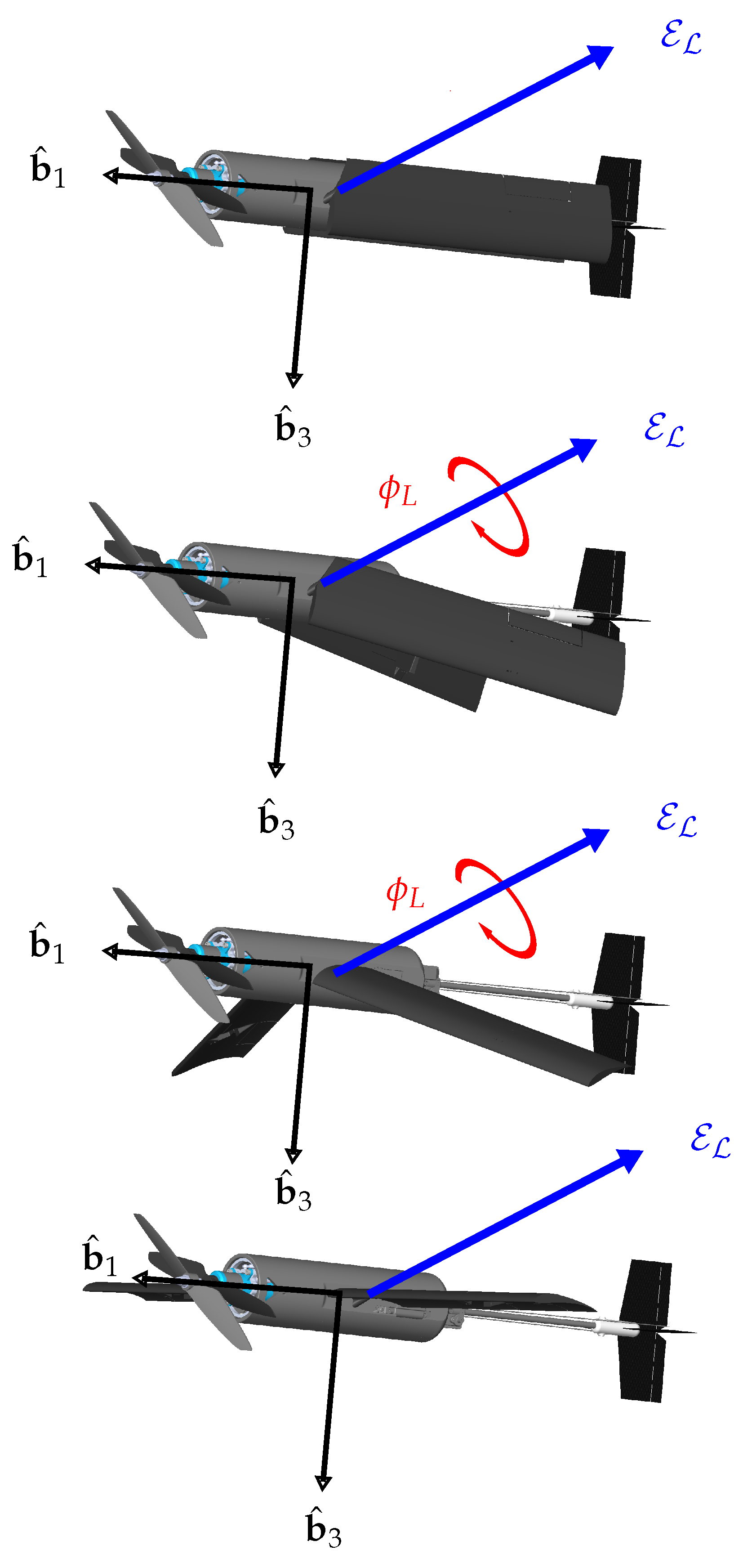
To model the wing-folding mechanism in the RCAS, a principal axis–angle method is implemented. The principal axis for each wing can be defined as follows: Let ${\mathcal{E}}_{\mathcal{L}}={\displaystyle \frac{1}{\sqrt{3}}}(-{\widehat{\mathbf{b}}}_1-{\widehat{\mathbf{b}}}_2-{\widehat{\mathbf{b}}}_3)$ be defined as the left wing principal axis, and let ${\mathcal{E}}_{\mathcal{R}}={\displaystyle \frac{1}{\sqrt{3}}}(-{\widehat{\mathbf{b}}}_1+{\widehat{\mathbf{b}}}_2-{\widehat{\mathbf{b}}}_3)$ be defined as the right wing principal axis, which are both expressed in the body coordinate system $\mathcal{B}$, as defined in a previous section. The principal angles corresponding to the left and right wing principal axis definitions, ${\varphi }_L$ and ${\varphi }_R$, respectively, are directly controlled to fold or unfold the wings. Starting from a wings-folded configuration, a negative right-handed rotation about ${\mathcal{E}}_{\mathcal{L}}$ from ${\varphi }_L=0°$ to ${\varphi }_L=-120°$ and a positive right-handed rotation about ${\mathcal{E}}_{\mathcal{R}}$ from ${\varphi }_R=0°$ to ${\varphi }_R=120°$ will result in both wings unfolding. As the wings unfold, the aerodynamic loads on the vehicle change due to the varying relative airflow, and this effect is included in the aerodynamic model. To avoid instantaneous non-physical motion with this implementation, the unfolding of the wings is approximated as a critically damped second-order system to imitate the realized vehicle. A side view of the wing-folding sequence is shown in Figure 5, where the left wing is shown rotating about its principal axis ${\mathcal{E}}_{\mathcal{L}}$ with principal angle ${\varphi }_L$.

3.1.6. Fuselage

The aerodynamics of the fuselage are modeled by incorporating lookup tables for three-dimensional lift, drag, and pitching moment as a function of the angle of attack, which were gathered from wind tunnel tests of the standalone fuselage model (discussed in [22]). They were imported into the RCAS as flat plate areas and dimensionalized using $L_{fuse}=f_{L}Q$, $D_{fuse}=f_{D}Q$, and $M_{fuse}=f_{M}Q$, respectively, where Q is the dynamic pressure. Interference modeling between the fuselage and the fixed-wing lifting surfaces is neglected at this time for simplicity.

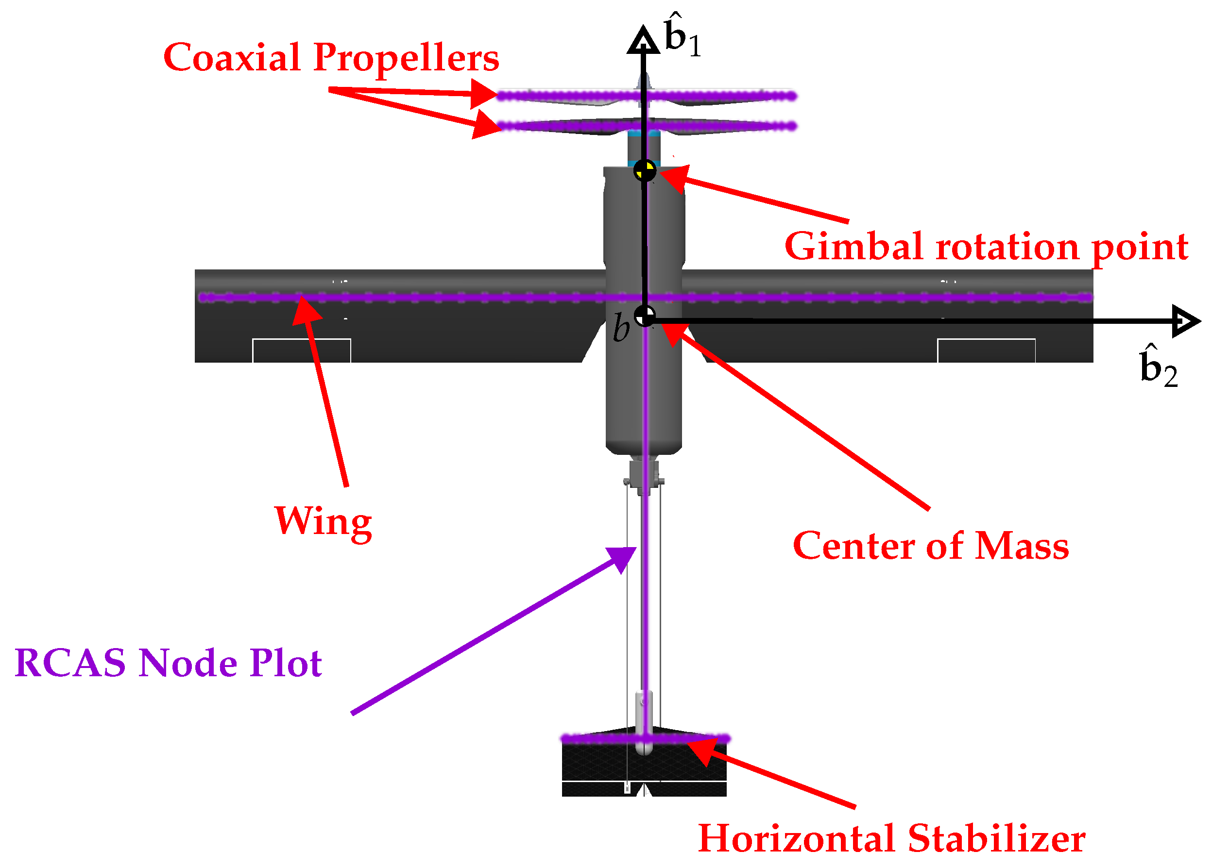
Implementation of the propellers, thrust-vectoring mechanism, wings, horizontal/vertical stabilizer, wing-folding mechanism, and fuselage completes the modeling for the Tailsitter. This can be visualized in the RCAS with a node plot of both structural and aerodynamic nodes which resembles the real vehicle, shown in Figure 6.

It should be noted that, while the major components of the Tailsitter are modeled, simplifications are made that limit the fidelity. More specifically, (1) all components are assumed to be rigid, (2) propeller–airframe interaction is neglected, and (3) the propellers use uniform inflow.

3.1.7. Mothership Definition

The chosen mothership that will air launch the Tailsitter is a full-scale conventional helicopter; however, it should be noted that this could also be a conventional fixed-wing aircraft or eVTOL (electric vertical take-off and landing) concept. The design of the helicopter was inspired by the Apache attack helicopter and includes an externally mounted launcher attached to the undercarriage of the fuselage. Following a similar definition process for the Tailsitter, a simplified full-scale helicopter is modeled in the RCAS. The assumed gross weight of the vehicle is 7000 kg (15,432 lb). The main rotor and tail rotor both include four rectangular untwisted blades which are all rigid. Inertia values for the blades and fuselage of the helicopter are assigned arbitrarily. The induced velocity model for both the main and the tail rotors is assumed to be uniform inflow. As the Tailsitter will be launched at a relatively high speed, it is assumed that the ALUAS will quickly escape the wake effects produced by the mothership’s rotors. Since the Tailsitter is launched with its wings folded, it is assumed that the wake exposure will minimally affect the Tailsitter’s dynamics. Hence, the interaction between the rotor wake and the Tailsitter is neglected, as it is deemed to be out of the scope of this study.

Each of the blades that make up the main rotor is allowed to flap and has a lag hinge. Pitch control is applied to mimic a swash plate, allowing for collective pitch, longitudinal cyclic, and lateral cyclic control to trim the aircraft for hover and forward flight.

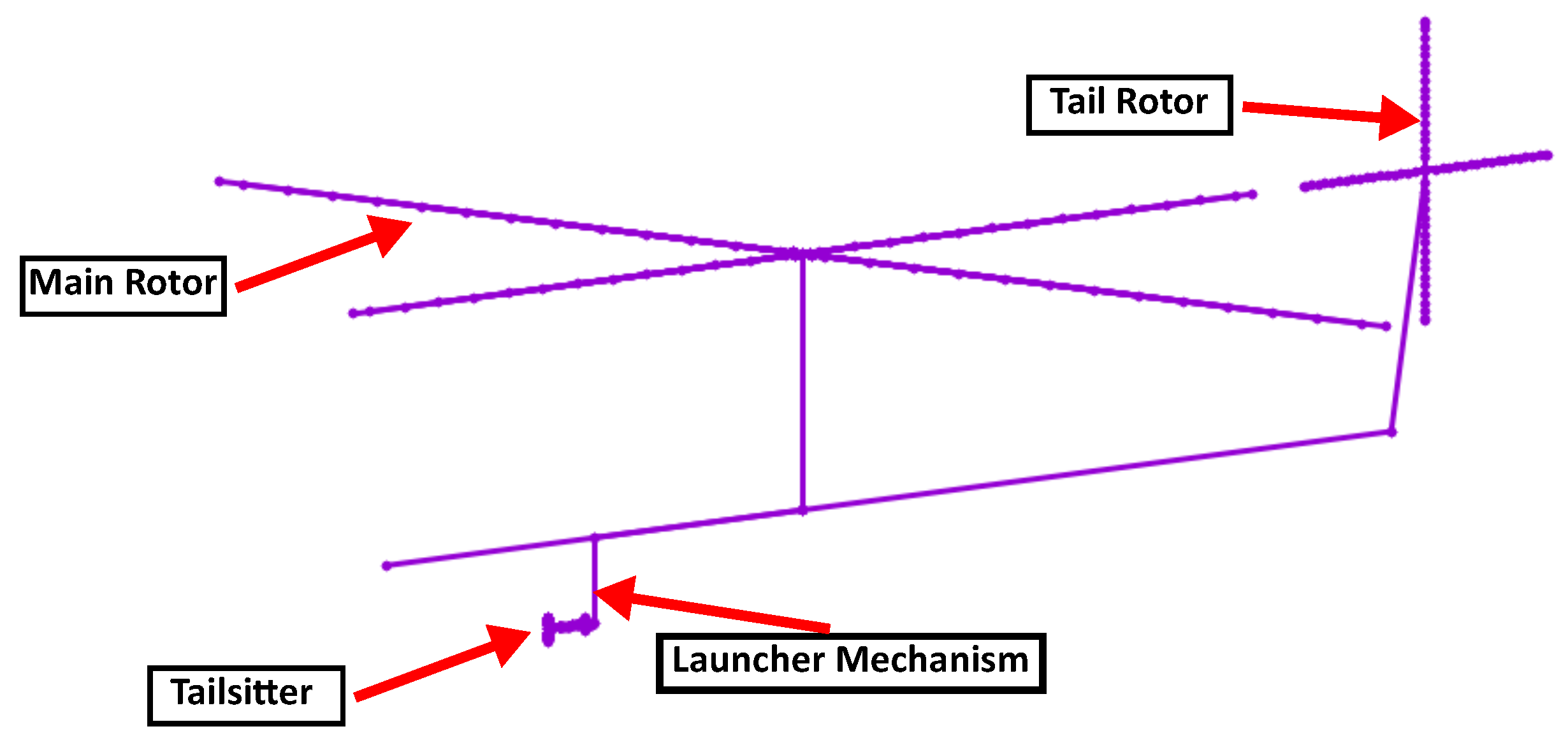
The launch mechanism mounted under the nose of the helicopter is capable of rotation about the Z and Y axis (yaw and pitch, respectively) to launch the Tailsitter in any arbitrary direction. At the beginning of an air launch maneuver, the Tailsitter is attached to the helicopter at the launcher node. When the Tailsitter is launched from the helicopter, the two systems can move independently of each other. To replicate a launch, an artificial external force is applied in the direction of the desired launch angle, which accelerates the Tailsitter to some forward velocity. The implementation of the helicopter mothership in the RCAS is shown in Figure 7, with the major components labeled. These include the main rotor, tail rotor, launcher mechanism, and Tailsitter UAS.

3.1.8. Control Systems

With the structural and aerodynamic components of the Tailsitter and mothership defined, the next step is to implement a control system to begin simulating various maneuvers.

To implement control laws, each maneuver must be assessed to determine which state variables need to be controlled. These states include the roll, pitch, and yaw angles, the roll, pitch, and yaw Euler rates, the flight path angle, and the inertial velocities of the Tailsitter. These are the variables necessary to achieve a lower level of control, i.e., the variables needed to perform isolated maneuvers as opposed to a full mission simulation, where trajectory following would also be required, adding further control variables such as the inertial positions x, y, and z.

The general control law used for all maneuver cases is Proportional–Integral–Derivative (PID). The control input, $U\left(t\right)$, is defined in the time domain by Equation (7):

$$U\left(t\right)=K_{P}e\left(t\right)+K_I\int e\left(\tau \right)d\tau +K_D{\displaystyle \frac{de\left(t\right)}{dt}}$$

(7)

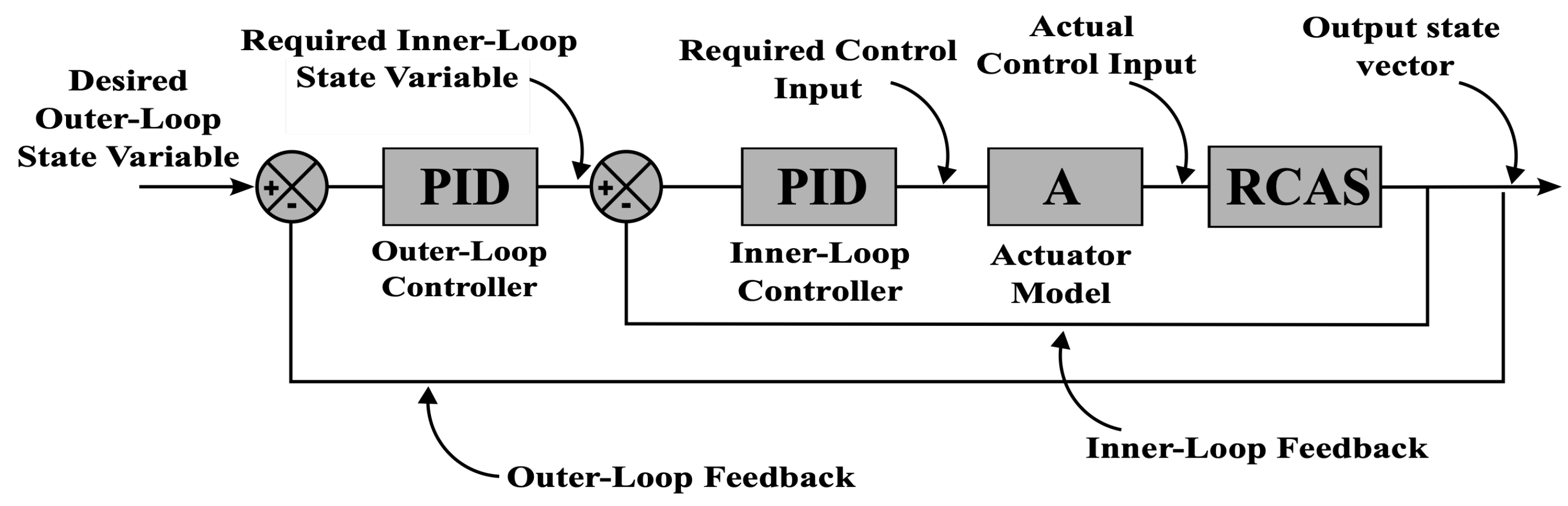
In this equation, $e\left(t\right)$ is the error signal, which is defined as $e\left(t\right)={\chi }_d\left(t\right)-\chi \left(t\right)$, ${\chi }_d\left(t\right)$ is the desired state, and $\chi \left(t\right)$ is the associated feedback state that is output from the simulation. Different values of each of the control gains, $K_P$, $K_I$, and $K_D$, are used in different cases and must be tuned in order for the vehicle to accurately follow the desired inputs. The architecture of the control system used for all maneuver cases is cascaded PID control. In general, this involves a series of PID feedback loops all connected to one another to generate a required control input. This cascaded architecture is used to improve overall performance. For most maneuvers in this work, the control architecture is outlined by Figure 8, where there are two PID loops, one for outer-level control and the other for inner-level control.

For many of the maneuvers, an actuator model is placed between the outputs from the inner-loop controller and the RCAS to capture the imperfections of a realized actuator and increase the fidelity of the simulation. The actuator models used for the present work are taken to be first- and second-order system models for simplicity.

For maneuvers where the aircraft is primarily operating in vertical flight, it is desired to control the roll, pitch, and yaw Euler angles, as well as the vertical velocity of the aircraft to hold altitude. The control loops associated with the desired Euler angles use the Euler angle rates for the inner loop. The vertical velocity control loop outputs directly to the throttle, ${\delta }_{{\Omega }_T}$ (i.e., simultaneously increases or decreases the upper and lower propeller angular velocities, ${\Omega }_u$ and ${\Omega }_l$). To hold altitude, the desired vertical velocity is commanded to be ${\dot{z}}_d=0$.

Depending on the pitch angle of the aircraft, the roll gimbal and differential propeller RPM may not always control the roll Euler angle and yaw Euler angle, respectively. If the vehicle is operating at a pitch angle of $90°$ (i.e., vertical flight), then the roll gimbal, which produces a torque about the ${\widehat{\mathbf{b}}}_3$ axis of the vehicle, will control the roll Euler angle. Similarly, the differential propeller RPM produces torque about the ${\widehat{\mathbf{b}}}_1$ axis of the vehicle and controls the yaw Euler angle. If the vehicle is operating at a pitch of $0°$, a torque about the ${\widehat{\mathbf{b}}}_3$ axis of the vehicle produced by the roll gimbal will then control the yaw Euler angle, and a torque about the ${\widehat{\mathbf{b}}}_1$ axis of the vehicle caused by the differential propeller RPM will control the roll Euler angle. This phenomenon is known as roll–yaw reversal and is further explained by Dooher et al. [8]. This problem is very relevant for the Tailsitter, as it is designed to transition between vertical flight and horizontal flight, where it must undergo large changes in pitch angle.

To avoid this problem, the control inputs are provided to the actuators by considering a pitch angle-invariant method. The inputs that are given to the three actuators include the gimbal roll angle (${\delta }_{{\zeta }_1}$), the gimbal pitch angle (${\delta }_{{\zeta }_2}$), and the differential propeller angular velocity (${\delta }_{{\Omega }_{diff}}$) and are given by Equation (8):

$$\left\{\begin{array}{c}{\delta }_{{\zeta }_1}\\ {\delta }_{{\zeta }_2}\\ {\delta }_{{\Omega }_{diff}}\end{array}\right\}=\left\{\begin{array}{c}sin\left(\theta \right)U_r+cos\left(\theta \right)U_y\\ U_p\\ -(cos\left(\theta \right)U_r-sin\left(\theta \right)U_y)\end{array}\right\}$$

(8)

Here, $U_r$, $U_p$, and $U_y$ are the outputs of the cascaded PID loops corresponding to the roll, pitch, and yaw Euler angles. Depending on the pitch angle ($\theta$), the formulation in Equation (8) provides a combination of the outputs from the roll and yaw cascaded PID loops to each of the control actuators, which are weighted by the value of the pitch angle. The main point of using this approach is to ensure that the vehicle’s roll and yaw Euler angles can be controlled during large changes in the pitch Euler angle, which occurs for the Tailsitter when performing a transition maneuver.

In general, propeller speed is changed because of either a differential torque requirement (${\delta }_{{\Omega }_{diff}}$) or a throttle requirement (${\delta }_{{\Omega }_T}$). With these contributions in mind, the upper and lower propeller angular velocities are then updated using Equation (9):

$$\left\{\begin{array}{c}{\Omega }_u\\ {\Omega }_l\end{array}\right\}=f\left\{\begin{array}{c}{\Omega }_{hover}+{\delta }_{{\Omega }_{diff}}+{\delta }_{{\Omega }_T}\\ -({\Omega }_{hover}-{\delta }_{{\Omega }_{diff}}+{\delta }_{{\Omega }_T})\end{array}\right\}$$

(9)

where $f(·)$ represents an actuator model, and ${\Omega }_{hover}$ represents the required control input for the aircraft to hover. Here, the upper propeller rotates counter-clockwise (positive), and the lower propeller rotates clockwise (negative). To account for this, control inputs are first applied to the magnitudes of each propeller angular velocity. The differential torque control input is added to the upper propeller velocity but subtracted from the lower propeller velocity. This way, their magnitudes are different depending on the value of ${\delta }_{{\Omega }_{diff}}$, which can be a positive or negative quantity. The equation for the lower propeller’s angular velocity is scaled by $-1$ to account for its clockwise rotation.

For vertical flight maneuvers, the vertical velocity in the ${\widehat{\mathbf{n}}}_3$ direction is controlled by increasing the throttle of both upper and lower propellers simultaneously with equal magnitude; there is no inner loop for this particular controller.

The transition maneuver to fixed-wing flight is treated as a longitudinal, three-degree-of-freedom maneuver, where the pitch angle is controlled using the gimbal mechanism. Once the transition is complete, the controller is switched to a flight path angle controller for fixed-wing flight, which uses different control gains and actuators. Moreover, when transitioning back to vertical flight, the pitch angle controller using the gimbal is re-enabled and an outer-loop velocity controller is enabled to ensure that the aircraft comes to a static hover.

The ground launch and air launch scenarios also need attitude control; however, to ensure that the aircraft is flying level, the flight path angle ($\gamma$) is used as a replacement for pitch angle ($\theta$). This is because a zero-degree pitch angle command may not correspond to a level flight condition. The control surfaces used for these two maneuvers are the ailerons, elevator, and rudder, which are conventional for fixed-wing aircraft. The roll angle of the aircraft is controlled by deflecting the ailerons, the flight path angle with the elevator, and the yaw angle with the rudder. A similar cascaded PID approach is utilized where the corresponding inner-loop state variables (for roll angle, flight path angle, and yaw angle) are the roll rate, pitch rate, and yaw rate, respectively.

Gains for all PID controllers are tuned through a trial-and-error process that starts with the inner-loop controller and then tunes the outer loop until the desired performance is achieved.

3.2. Hover Testing

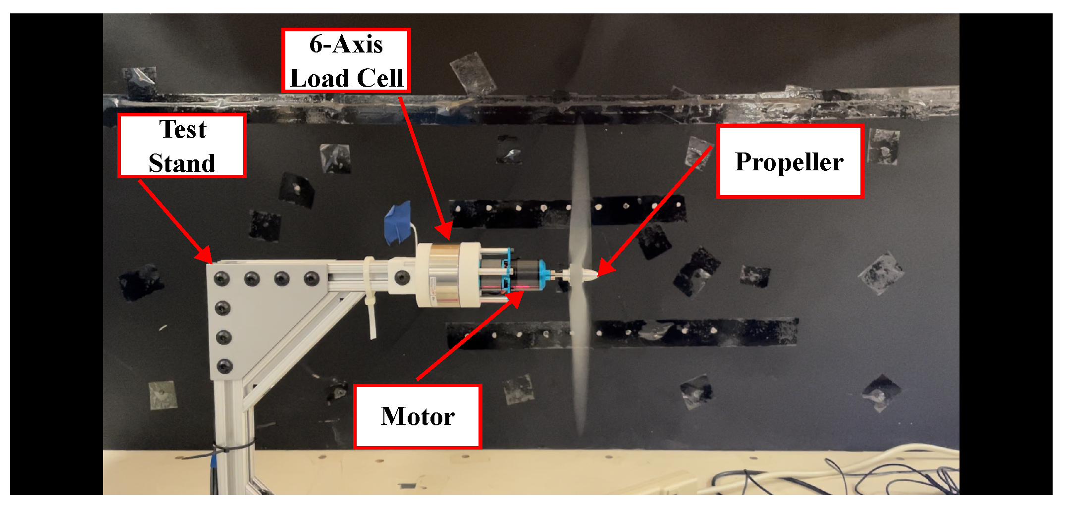
Meaningful simulations require accurate prediction of actuator behavior. In particular, predictions of the propeller’s dimensional thrust and torque from the flight dynamics simulation must capture the physical behavior of the vehicle with reasonable accuracy. To validate these predictions, the thrust and torque from a single propeller model in the RCAS are compared with results from a static single-propeller experiment. The experimental setup displaying the propeller/motor mount on the test stand is shown in Figure 9. The thrust and torque are measured using a 6-axis load cell, and the propeller angular velocity is measured using a laser tachometer.

4. Results

4.1. Propeller Model Validation

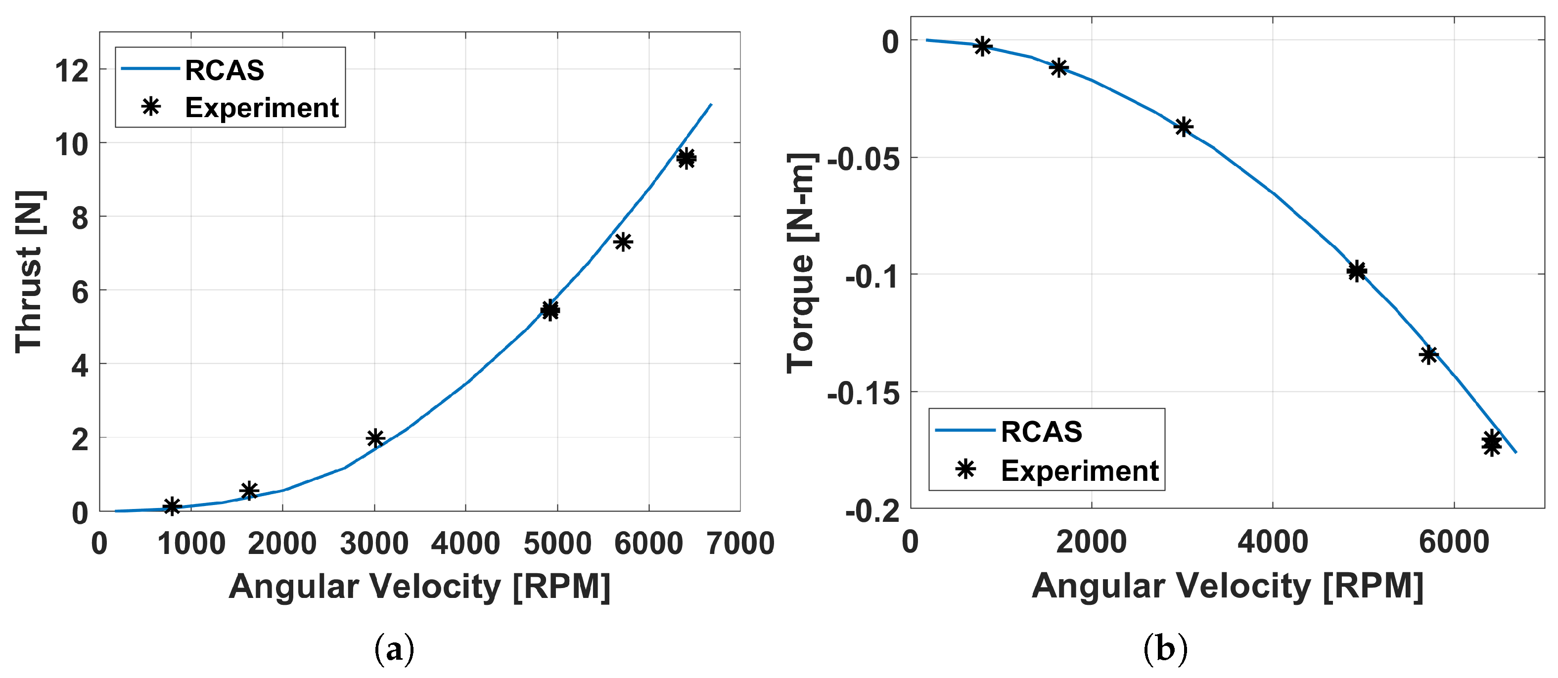
The thrust and torque were measured at different propeller rotational speeds in a hovering condition. With this experimental data, validation of the RCAS single-propeller model was performed, where the uniform inflow model was selected in the RCAS. This inflow model was selected as it is used later during maneuvering flight simulations. In Figure 10, the dimensional thrust (Figure 10a) and torque (Figure 10b) of the propeller are compared between the RCAS and the experiment at different propeller speeds (RPM). The RCAS predictions show good agreement with the experiment for both thrust and torque, where the root-mean-squared error (RMSE) is 0.4 N for thrust and 0.005 N-m for torque. As the Tailsitter has coaxial propellers (the upper and lower propellers are identical), the associated coaxial model in the RCAS considered upper-to-lower-propeller interference, as outlined in the methodology. Finally, the thrust and torque from the upper and lower propellers were summed together to determine the total thrust and torque acting on the aircraft.

4.2. Maneuver Simulations

Using gathered wind tunnel data (see [22] for more details) to correct the RCAS flight dynamics model and enforce physical constraints, the model was then used to simulate various maneuvers that ALUASs are designed to perform. The simulations began with the transition maneuver from hover to horizontal flight, followed by ground launch, a nominal air launch, and, finally, a non-ideal air launch consisting of asymmetric wing unfolding.

Depending on the maneuver, aerodynamic force coefficients came directly from wind tunnel data or they were computed by the RCAS lifting line-based aerodynamic model, which was corrected empirically.

The transition maneuver used the wind tunnel data for the full aircraft for the lift, drag, and pitching moment [22]. As the Tailsitter was likely to encounter high angles of attack while performing this maneuver, wind tunnel tests were conducted on a canonical model of the full aircraft that included the wings, fuselage, and stabilizer. During testing, the angle of attack was swept from $\alpha =-15°$ to $\alpha =105°$, and the associated lift, drag, and pitching moment coefficients were measured. As the effects of stall are difficult to model, the RCAS flight dynamics model relied on the wind tunnel test data to compute the aerodynamic force seen by the Tailsitter. However, the coaxial propeller air loads were still computed using blade element theory. The contribution to the net moment about the center of mass due to the elevator deflection was also still modeled using Equation (5), as outlined by Nelson [30].

The ground launch and air launch maneuvers used the wind tunnel fuselage data for lift, drag, and pitching moment lookups while using the corrected RCAS aerodynamics model to predict airloads for the main wing and horizontal and vertical stabilizers. One of the main characteristics of the ground launch and air launch maneuvers is the Tailsitter’s ability to be launched from a tube and go from a folded to an unfolded configuration and enter horizontal flight. Due to the lack of wind tunnel data during wing deployment, this work relied on RCAS aerodynamic predictions to determine the effects of the wing unfolding on the aircraft, with the goal of predicting the trend accurately. Furthermore, any contributions to aerodynamic moments from control surface deflections were modeled by the RCAS.

A summary of how wind tunnel (WT) data was incorporated into the RCAS for each maneuver is shown in

Table 2. Wind tunnel data incorporation during various maneuvers.

Maneuver	WT Contribution	RCAS Contribution
Transition	Full Aircraft Lookup	Propeller Model
Ground Launch	Fuselage and Empirical Correction	Propeller and Wing Model
Air Launch	Fuselage and Empirical Correction	Propeller and Wing Model
Asymmetric	Fuselage and Empirical Correction	Propeller and Wing Model

.

The equations of motion were integrated using the Newmark-beta method [31]. All simulations were run at a constant time-step of $dt=0.0005$ s. Further information about the RCAS is given by Saberi et al. [28] and Hasbun et al. [29].

4.2.1. Case 1: Transition Maneuver

Simulation of the transition maneuver that takes the aircraft from hover to forward flight and back to hover is discussed in this section. This maneuver is of great importance because it essentially acts as the bridge between vertical flight and horizontal flight.

Prior to beginning the transition maneuver, the vehicle is trimmed in hover with its wings already unfolded at a wing principal angle of $120°$. The trim is based on finding the propeller angular velocity that ensures zero net force in the vertical (z) direction, which was found to be approximately $\Omega =5800$ RPM. The overall maneuver can be broken into three distinct phases: the initial transition from hover to horizontal flight, level flight trim, and, finally, the transition back to hover from horizontal flight.

The transition from hover to forward flight begins by commanding a ramp to a pitch angle ($\theta$) of $0°$ as well as simultaneously increasing the angular velocities of both propellers to a constant value of ${\Omega }_u={\Omega }_l=7000$ RPM. This increase in throttle is done to (1) quickly transition the aircraft to horizontal flight and (2) reduce its angle of attack to avoid unnecessary flow separation, which could disrupt the transition. When the desired pitch angle is $0°$ ($t=6$ s), the vehicle is commanded to a flight path angle of $0°$, which corresponds to level horizontal flight. At this point, a switch in pitch control is made from gimbal deflection (${\delta }_{{\zeta }_2}$) to elevator deflection (${\delta }_e$), to account for the propeller’s effectiveness decrease due to the aircraft gaining forward speed. The aircraft remains in a level flight condition for approximately 5 s, cruising at a speed of approximately 20 m/s.

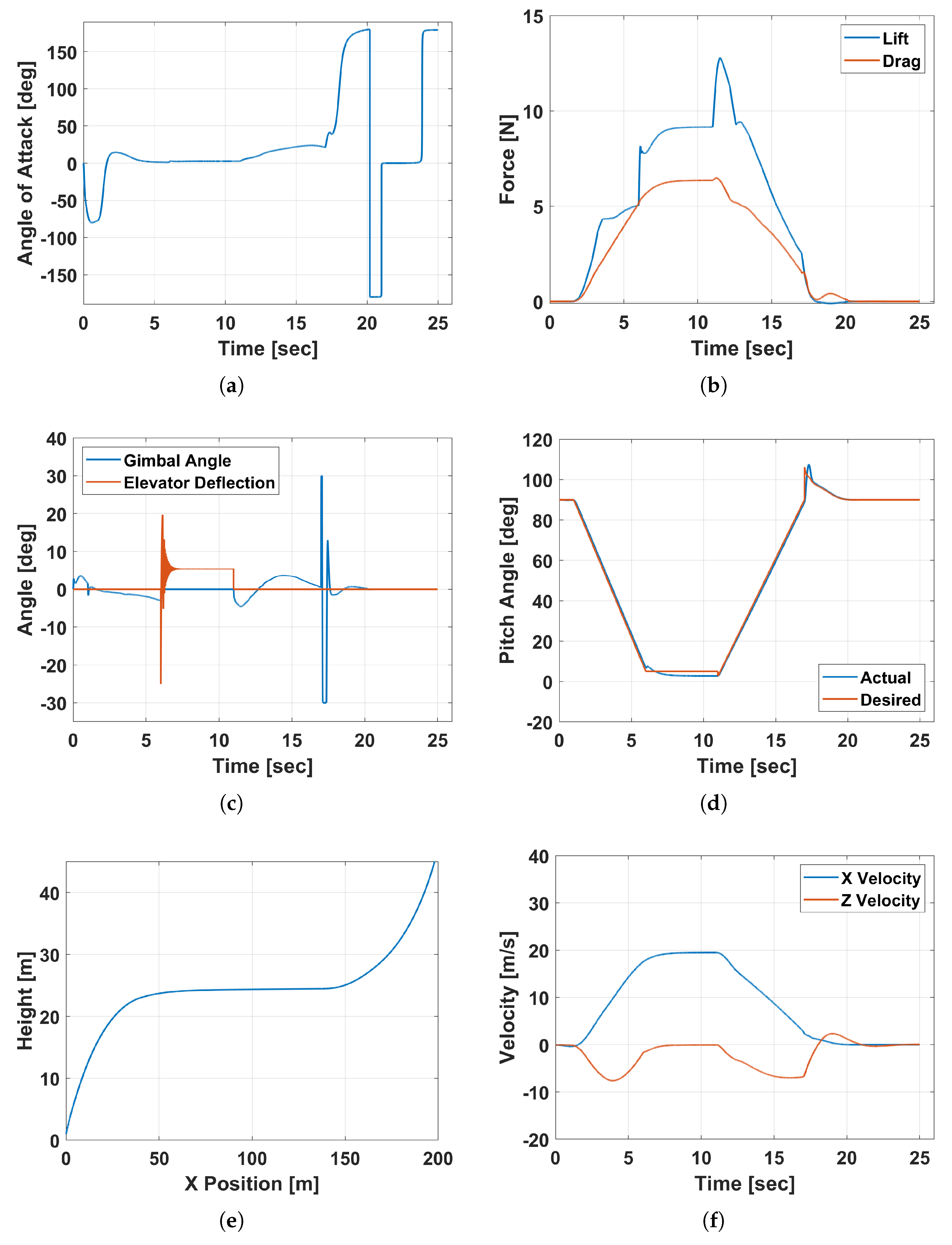
To transition back to hover from horizontal flight, the throttle of the upper and lower propeller is simultaneously decreased back to the value obtained for hover, and pitch angle control is switched back from the elevator to the pitch gimbal. A ramp command is then provided to take the aircraft back to a pitch angle of $90°$, which corresponds to hover. During this ramp, the angle of attack of the aircraft, shown in Figure 11a, begins to increase and causes an increase in both lift and drag, as shown in Figure 11b. This increase in aerodynamic force helps to slow the aircraft. Notably, the angles of attack observed are very large when transitioning back to hover and would be out of range of the RCAS’ aerodynamic predictions. This adds to the reason for incorporating wind tunnel data [22], as it helps to accurately predict the vehicle’s dynamics. To ensure that the aircraft comes to a complete stop, outer-loop velocity PID controllers for the x and z inertial velocities are implemented on top of the existing cascaded control loop for the pitch angle. To rapidly slow the vehicle to a halt, the velocity controller requires the thrust vector to quickly deflect to a large angle of $30°$ and oppose the forward motion, which is shown in Figure 11c. This results in the aircraft returning to a stationary hover, which concludes the maneuver.

Figure 11d shows the desired pitch angle versus the vehicle’s actual pitch angle as a function of time. The vehicle is able to track the desired pitch angle commands for the decreasing and increasing pitch ramps.

The position of the vehicle during the transition maneuver is shown in Figure 11e, which plots the inertial height (negative of inertial z position) as a function of the inertial x position. The initial transition from hover to horizontal flight (cruise) shows the vehicle ascending as well as translating forward in the x direction as it enters level flight. When it transitions back to hover, there is a further increase in height as it comes to a halt. This is due to the increase in the angle of attack as the aircraft pitches upward, which causes an increase in lift force (Figure 11b).

The inertial velocities during the transition maneuver are shown in Figure 11f, which shows the vehicle initially in hover, increasing speed during transition, then entering into a level flight condition at approximately $t=6$ s, where the z velocity is 0 m/s. Finally, the aircraft decelerates and resumes hovering flight at the end of the maneuver, with both the x and z inertial velocities coming to 0 m/s. Note that, as the z axis points downwards, the negative z velocity seen in Figure 11f denotes a climb.

To achieve the desired pitch angle ($\theta$) and flight path angle ($\gamma$) during the transition, two different control actuators are used. The desired pitch angle is mapped to the pitch thrust vector using cascaded PID control. However, as forward velocity increases during the transition, the pitch thrust vector loses effectiveness. Therefore, when the vehicle is commanded to a flight path angle of $\gamma =0°$, the conventional fixed-wing elevator control surface is utilized and the pitch thrust vector angle is set to zero. When transitioning back from horizontal flight to hover, the pitch thrust vector is re-enabled to control the pitch angle of the aircraft and the elevator deflection angle is set to zero. Figure 11c shows the usage of both the pitch thrust vector and the elevator at different parts of the transition maneuver.

4.2.2. Case 2: Ground Launch Maneuver

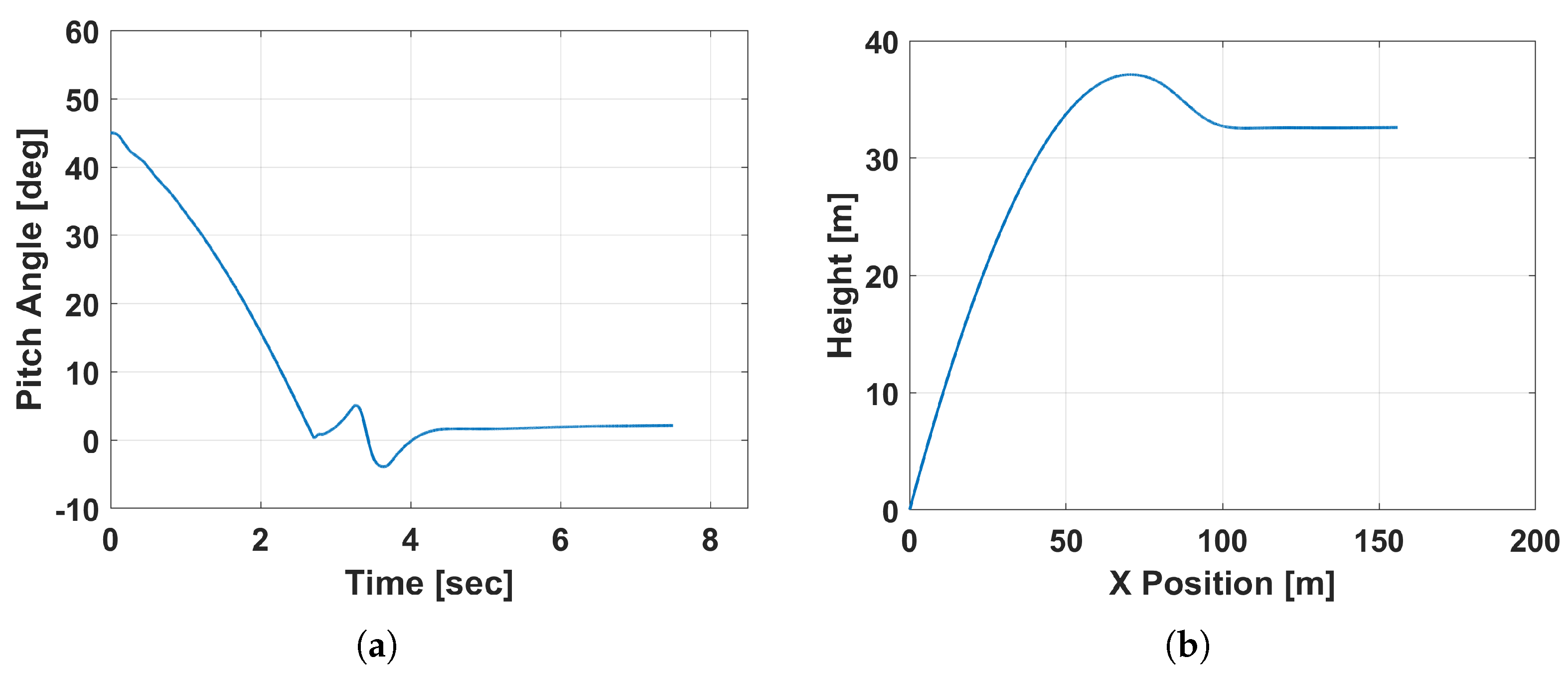
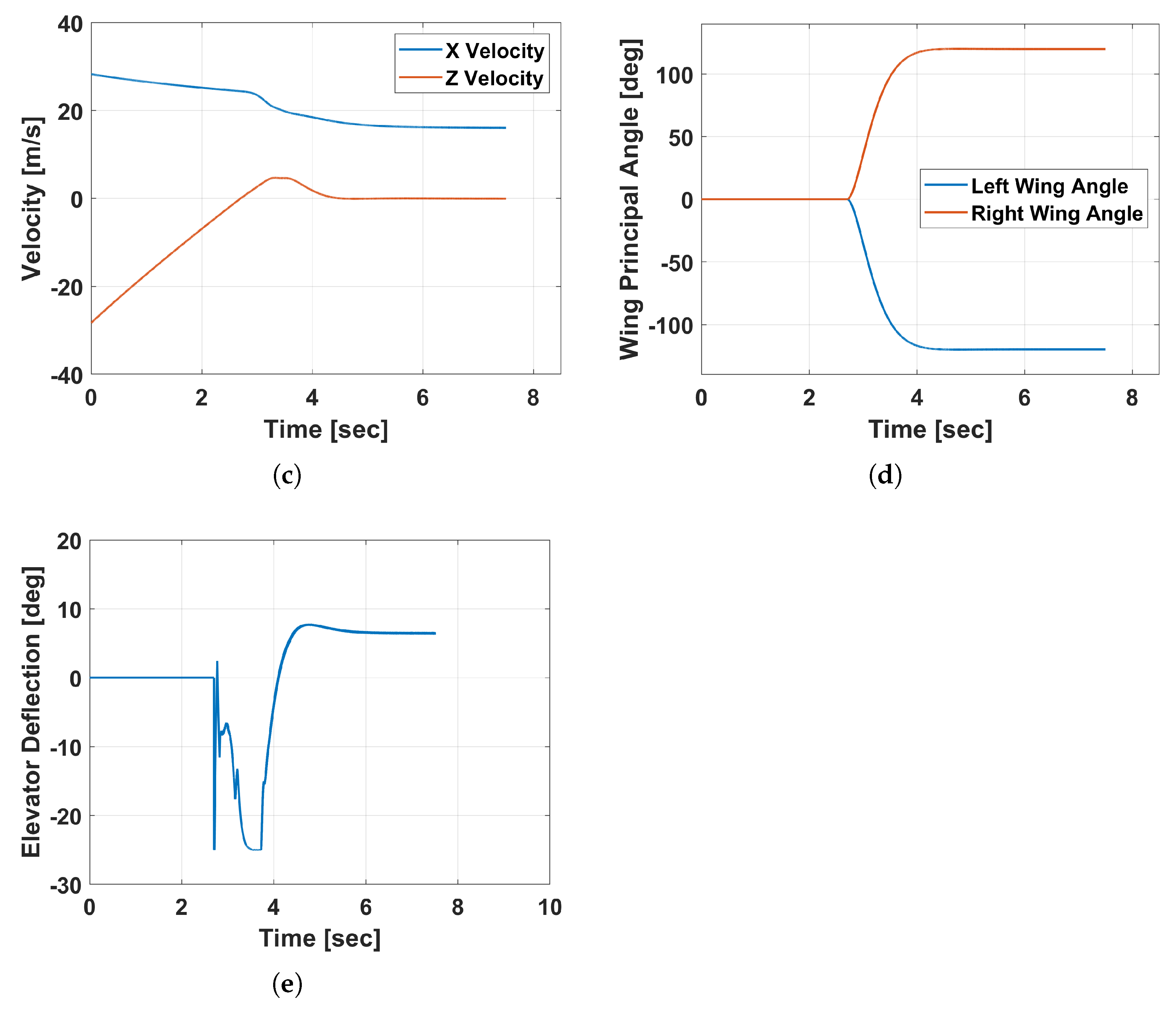
The ground launch maneuver begins with the aircraft in a wings-folded configuration. In a real case, the aircraft would be deployed from a launcher. To replicate this ballistic launch in simulation, the aircraft is subjected to an initial velocity of 40 m/s and a launch angle of $45°$. When launched, the aircraft remains as a projectile in an uncontrolled ascent. When the aircraft reaches the apex of its projectile motion (i.e., when the inertial vertical velocity component, $\dot{z}\left(t\right)$, becomes zero), the wings are unfolded and the propellers are spun up to ${\Omega }_u={\Omega }_l=5834$ RPM simultaneously. A zero-degree flight path angle ($\gamma$) is then commanded, and the vehicle eventually enters a level horizontal flight configuration. Figure 12a shows the pitch angle of the vehicle as a function of time. Here, the vehicle starts at an orientation of $45°$, which slowly decreases with time. At approximately $t=2.7$ s, the vehicle hits the apex of projectile motion, where it deploys the wings and spins up the propellers. This is shown in the position plot Figure 12b, where the curve hits a local maximum, and the velocity plot Figure 12c, where the z velocity goes to 0 m/s.

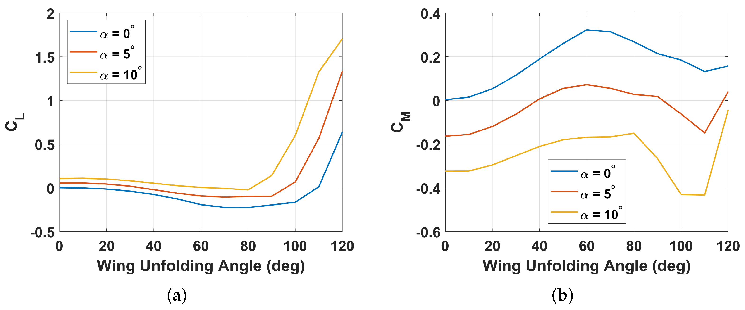
At the apex, the wings begin to unfold; however, it is not until approximately $t=4.5$ s that the wings are fully unfolded to a principal angle (${\varphi }_R$) of $120°$, as shown in Figure 12d (Note, the notation ${\varphi }_R$ is used to describe the wing folding angle of the right wing. In this case the left wing folds in sync with the right wing, ${\varphi }_L=-{\varphi }_R$). Because of this, there is a transient phase where the airloads are rapidly changing, causing the vehicle to drop further in pitch angle and, hence, altitude. This can be explained by examining Figure 13, which displays the aircraft’s lift coefficient varying with wing principal angle (${\varphi }_R$) in Figure 13a, as well as the pitching moment in Figure 13b. For both the lift and pitching moment, the angle of attack is also varied between $\alpha =0°$ and $\alpha =10°$. It can be observed that, as the wings begin to unfold (${\varphi }_R=0°$), the aircraft’s lift decreases for all angles of attack. It is only towards the end of the unfolding procedure that the wings gain effectiveness (towards ${\varphi }_R=120°$), as evidenced by the large increase in the lift coefficient. Furthermore, for positive angles of attack, the pitching moment for the most part is always negative. In other words, a nose-down moment is being applied during the wing-unfolding process. As the angle of attack throughout the ground launch is always positive, the aircraft experiences a negative pitching moment up until the wings are fully deployed.

The pitch angle transience in Figure 12a can be explained further by examining the elevator deflection shown in Figure 12e. As the vehicle primarily operates in horizontal flight during this maneuver, only the elevator is used to control the pitch of the aircraft. The thrust vector remains un-deflected for the entirety of the maneuver. When the elevator control is activated at the apex of the trajectory, it rapidly deflects upward (negative elevator angle) in an attempt to quickly bring the aircraft to $\gamma =0°$. Note that an upward deflection of the elevator means a positive moment is being generated about the aircraft’s center of gravity, which results in an increase in pitch angle and angle of attack at approximately $t=3$ s. As the wings continue to unfold and pass approximately ${\varphi }_R=80°$, the nose-down pitching moment caused by the wing unfolding becomes larger in magnitude and causes the elevator to saturate at ${\delta }_e=-25°$. The elevator deflection remains negative until approximately $t=4$ s, when the wings almost fully deploy and the nose-down pitching moment rapidly decreases in magnitude.

At $t=5$ s, the aircraft enters a 17 m/s cruise. Here, the wings have fully unfolded and the controller is able to find the elevator deflection such that the flight path angle is zero, which is approximately 7.5°.

4.2.3. Case 3: Air Launch Maneuver

The air launch maneuver consists of the Tailsitter being launched from a larger full-scale aircraft that acts as a mothership. In general, the mothership can be a fixed-wing aircraft or rotorcraft. For this example, a full-scale six-degree-of-freedom helicopter is modeled in the RCAS with a launch mechanism capable of both orienting and propelling the Tailsitter at some initial launch angle and speed, respectively. To show the versatility of the Tailsitter, the helicopter is trimmed for forward flight at a speed of 15 m/s, where it will launch the Tailsitter at a $-45°$ launcher pitch angle. A prescribed force will then propel the Tailsitter as a projectile. Under these conditions, the Tailsitter will not only see airspeed due to being launched from the tube, but it will also have to handle the effect of the airspeed induced by the helicopter’s forward motion. For simplicity, the effect of the helicopter main rotor wake is not included in this analysis. Due to the higher airspeed experienced by the vehicle, the usage of the thrust-vectoring mechanism does not significantly contribute to the overall controllability of the vehicle. In this case, only the elevator is used to control the aircraft, similar to the ground launch scenario.

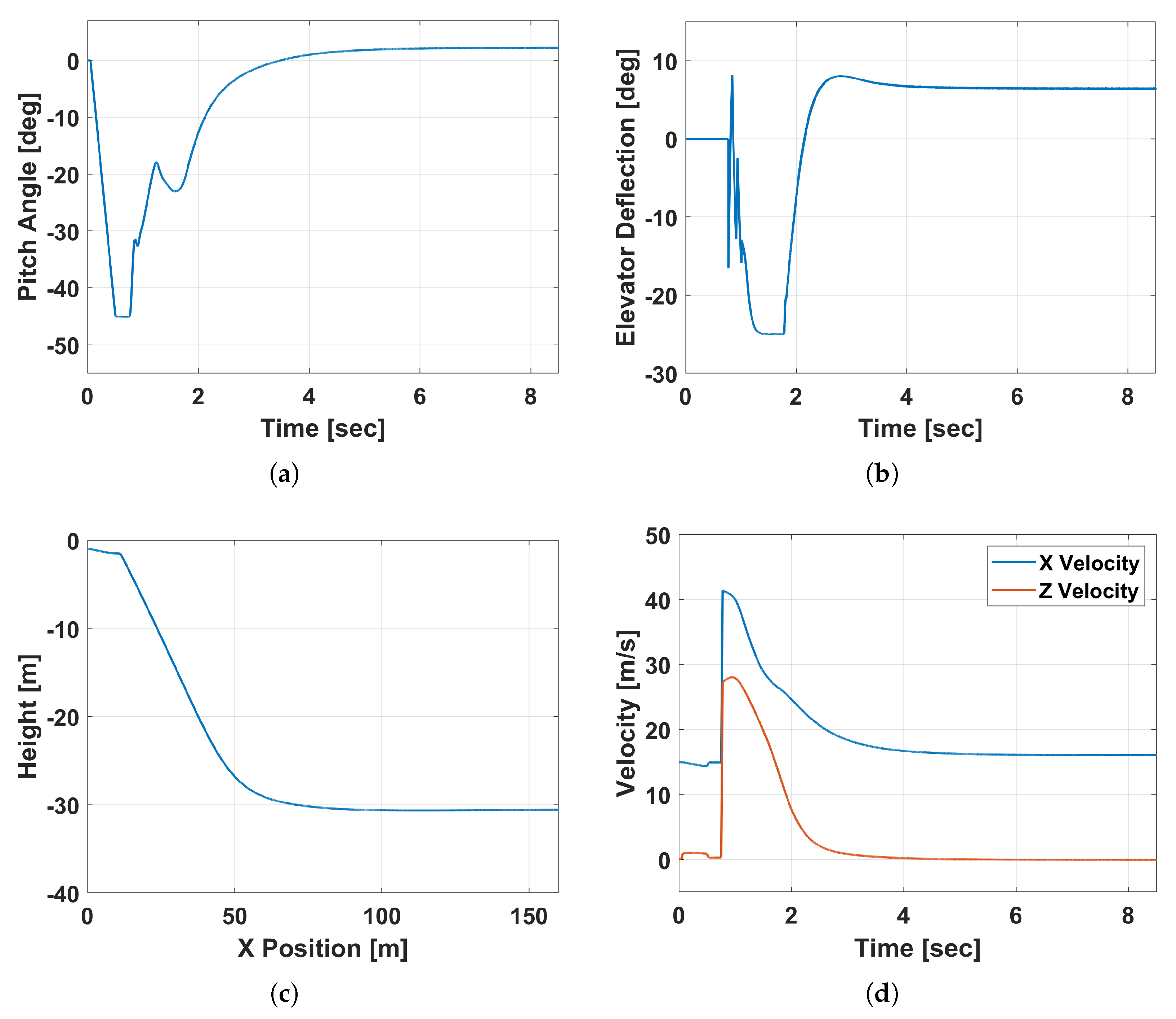
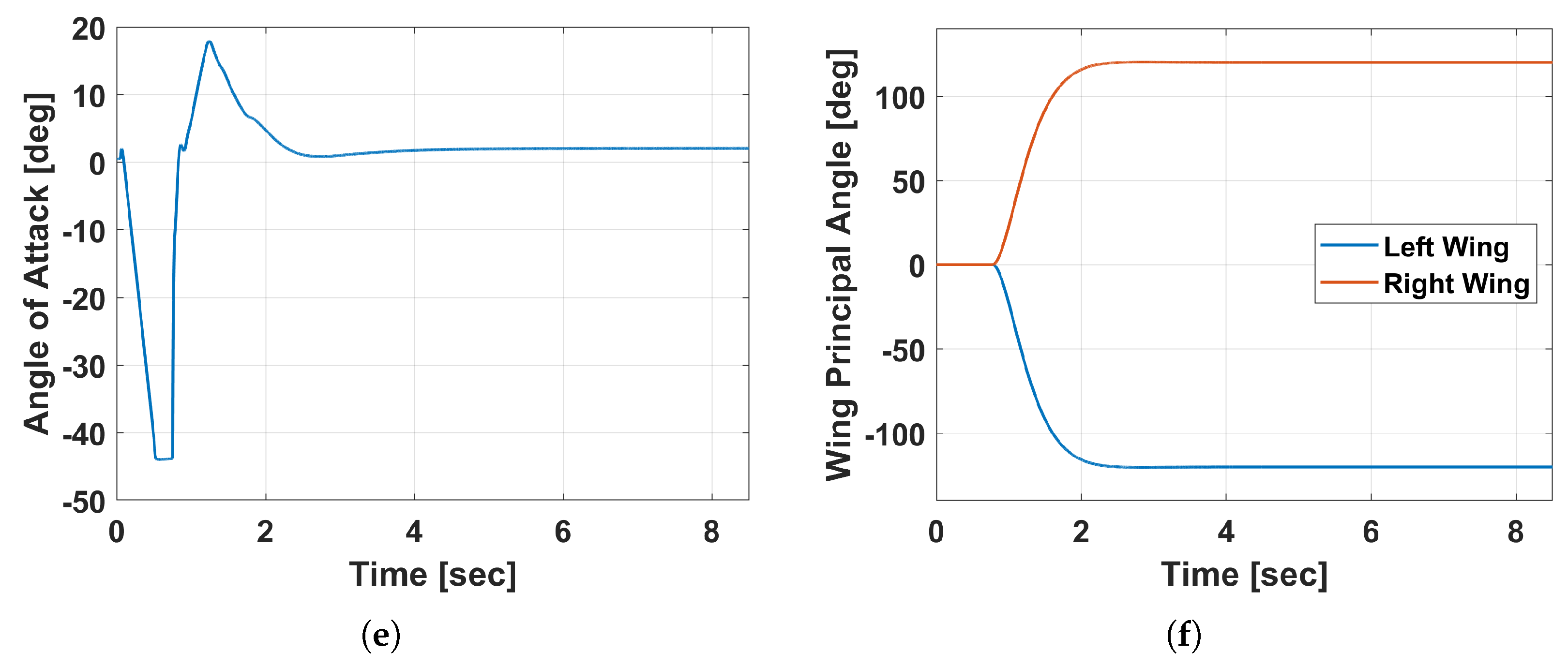
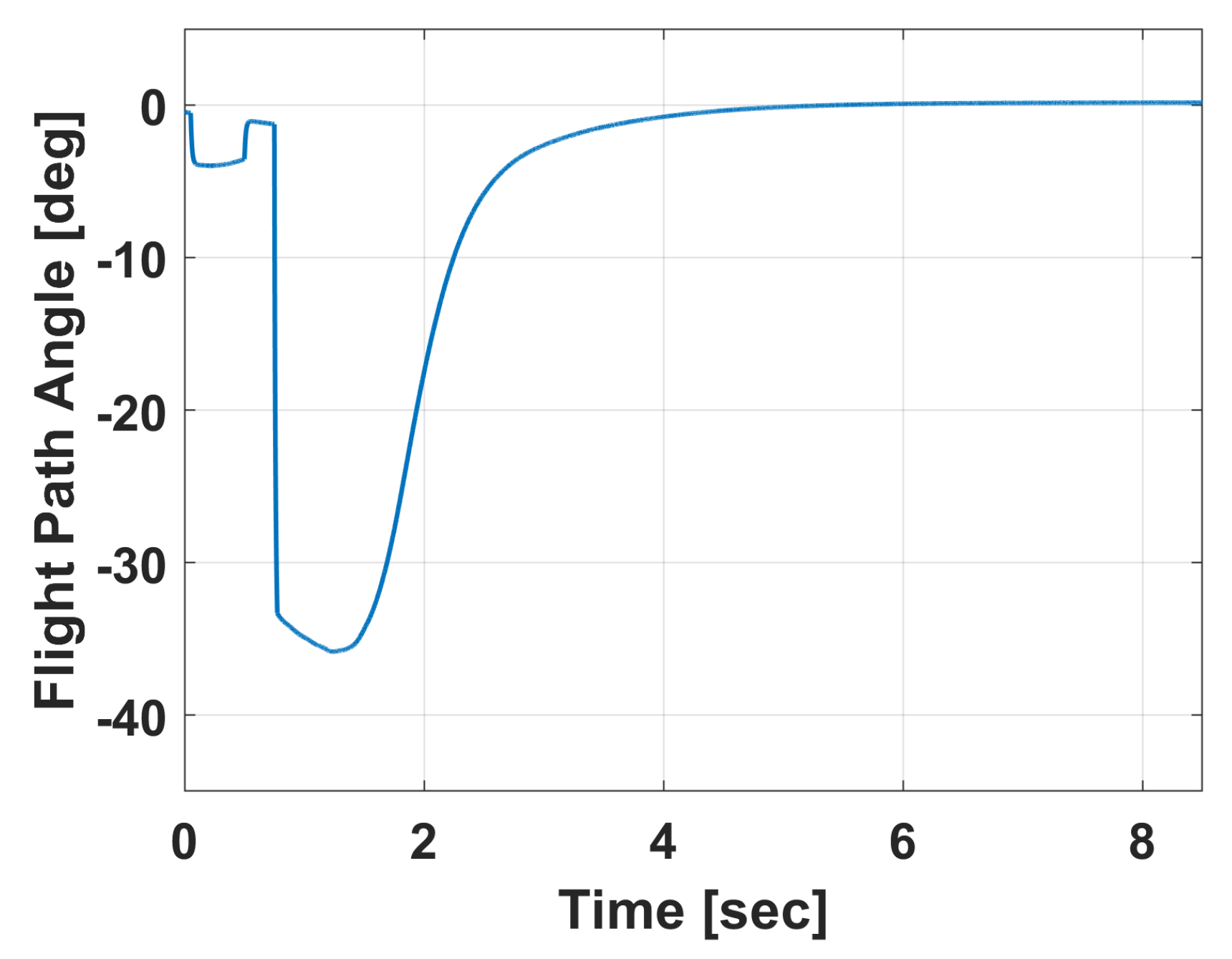
To begin the maneuver, the launcher is pitched downward to $-45°$ relative to the mothership, as shown in Figure 14a, which plots the pitch angle of the Tailsitter as a function of time. At approximately $t=0.75$ s, the Tailsitter is launched from the moving helicopter. Immediately upon launching at $t=0.75$ s, the flight path angle controller is enabled and begins to deflect the elevator to orient the vehicle to fly level at a flight path angle $\gamma =0°$ (Figure 15). Meanwhile, at $t=0.75$ s, immediately after launching, the propellers are simultaneously spun up to ${\Omega }_u={\Omega }_l=5834$ RPM and the wings begin to deploy. The almost immediate increase in pitch angle that is shown in Figure 14a can be attributed to the elevator control surface deflection, which is shown in Figure 14b, as it is trying to quickly orient the Tailsitter to fly level.

The position of the Tailsitter is shown in Figure 14c. The aircraft descends almost 30 m before leveling out for horizontal flight, due to the initial downward velocity from the launch. The inertial velocity, shown in Figure 14d, begins to decrease in the x direction due to the drag force on the aircraft. After the wings are fully unfolded at approximately $t=2.5$ s, the aircraft reaches a cruise speed of approximately 17 m/s.

The angle of attack of the Tailsitter is shown in Figure 14e. This essentially gives a summary of the airloads on the aircraft during the maneuver. Initially, the angle of attack matches the value of the Tailsitter’s pitch angle; however, after launch, it rapidly increases. The maximum angle of attack occurs during the wing-unfolding sequence.

The wing-unfolding angles are shown in Figure 14f. Similar to the ground launch scenario, midway through the deployment of the wings, the pitch angle decreases and then starts to constantly increase when the wings are close to being fully unfolded at approximately $t=2$ s. The fully unfolded scenario at approximately $t=2.5$ s represents the state when the aircraft is most controllable, and the flight path angle controller is then easily able to bring the aircraft to level flight, which is shown in Figure 15, where the flight path angle tends to $0°$.

The required elevator deflection for the air launch scenario is shown in Figure 14b. Immediately after the deployment, there are high oscillations in the required elevator deflection similar to in the ground launch case, as there is a large error between the desired and the actual flight path angle. For almost half a second, the elevator deflection hits its maximum value of $-25°$ (control saturation), indicating that the trailing edge of the elevator is pointing upward. In other words, the control system is trying to produce a nose-up moment. As the angle of attack is positive during the wing-unfolding procedure, the pitching moment on the aircraft is negative (nose-down), as seen in Figure 13b. Similar to in the ground launch, the elevator struggles to oppose the nose-down pitching moment produced by the wings unfolding and saturates for a period of time. After the wings deploy, the elevator is able to trim the aircraft for level flight at a deflection of approximately $7°$.

4.2.4. Case 4: Air Launch with Asymmetric Wing Deployment

After the Tailsitter is launched from its mothership, the wings are ideally unfolded symmetrically. However, this is unlikely to be true for the realized aircraft since there are separate actuators for unfolding each wing. Departing from the ideal cases shown before, simulations are now performed for cases where the wings do not begin deployment at precisely the same time. These simulations have been extended from three degrees of freedom (3-DOF) to 6-DOF to capture the effects of the non-zero roll moments that can be seen as a result of asymmetric wing deployment. To this end, the Tailsitter is once again air launched from its helicopter mothership, but, this time, the right wing begins to deploy some time period after the left wing begins to deploy. For simplicity, the vehicle is launched parallel with the helicopter’s longitudinal axis (i.e., no deflections of the launch mechanism) with the helicopter in hover.

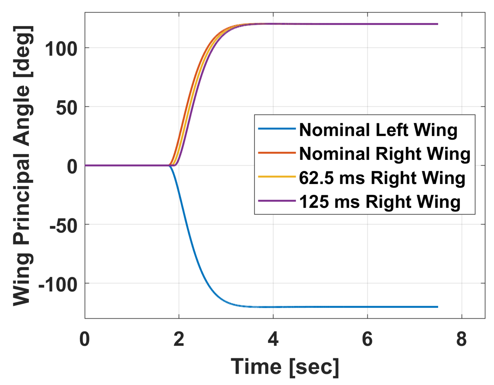
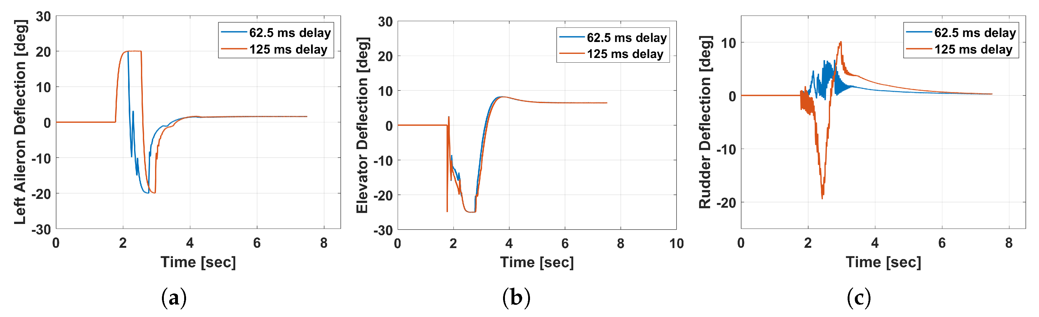
Two scenarios are explored, one where the right wing starts to deploy $62.5$ ms after the left wing starts to deploy, and a second scenario where there is a longer delay of 125 ms. These scenarios are visualized in Figure 16. For reference, time histories of the left and right wing-unfolding angles (principal angles) are shown for the “nominal” case where they unfold at the exact same time. Next, the wing-unfolding angle time history is shown for the two scenarios where the right wing begins to unfold slightly after the left wing for the $62.5$ ms and 125 ms cases.

It should be noted that the rate of deployment of the wings is kept constant for both cases. To complete these new 6-DOF maneuvers, aileron and rudder fixed-wing control surfaces must be used to correct any disturbance in roll and yaw Euler angles.

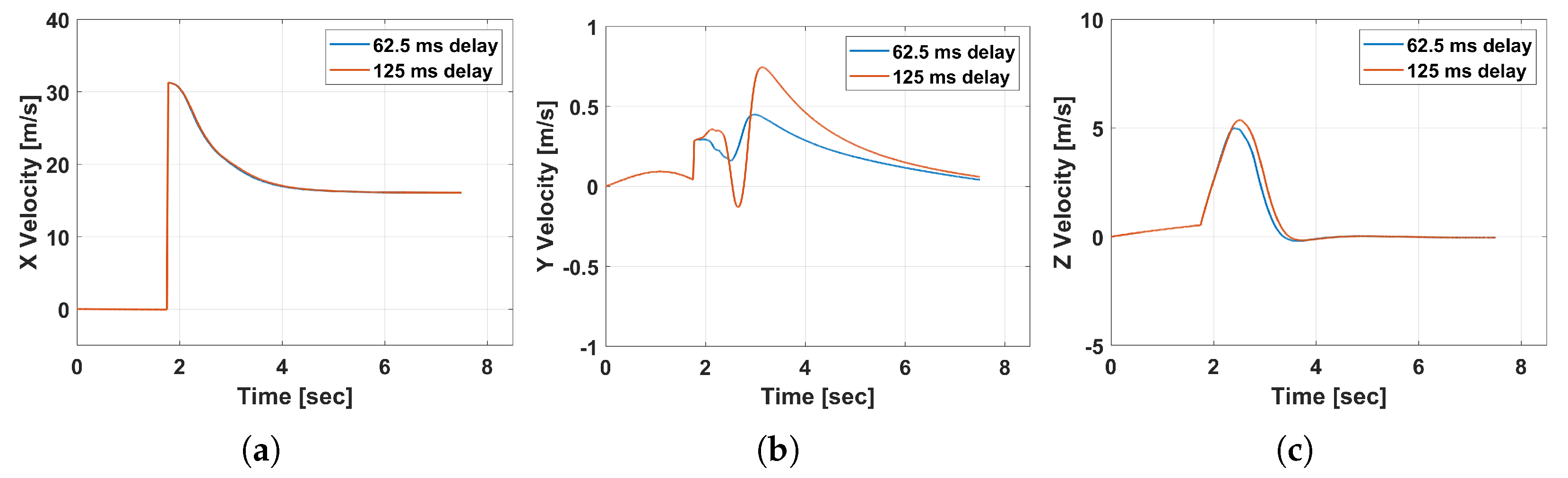
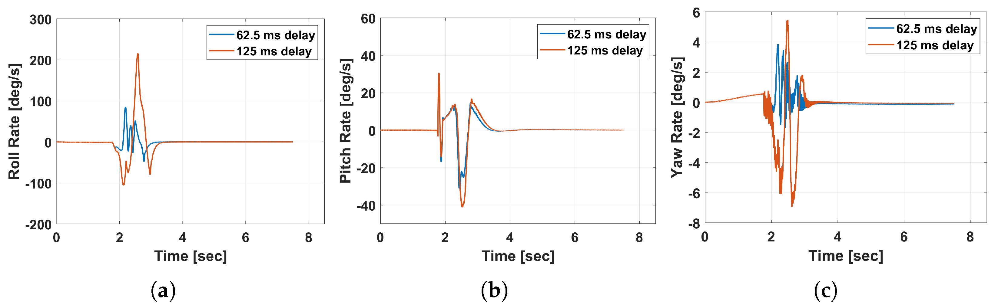
The inertial velocities of the Tailsitter are shown in Figure 17, where the x, y, and z velocities are displayed in Figure 17a, Figure 17b, and Figure 17c, respectively. At $t=1.75$ s, the Tailsitter is launched from the mothership, reaching a forward speed of almost 30 m/s for both wing-unfolding scenarios. Immediately after the launch, the left wing begins to unfold, which is shortly followed by the right wing. The asymmetry in lift for both cases induces a negative roll rate on the aircraft due to the way the wing unfolds, which is shown in Figure 18a. In other words, at the beginning of the unfolding procedure, the sectional angle of attack is negative on the left wing, which produces a negative lift, creating a negative roll rate. This is visualized in Figure 13a, which displays the aircraft’s lift coefficient as a function of the wing-unfolding angle (principal angle). The aircraft’s pitch rate in Figure 18b is smaller than the induced roll rate for both the $62.5$ ms and 125 ms cases. During wing unfolding, the aircraft sees a predominately nose-down pitching moment, as shown in Figure 13 for positive angles of attack. This results in the induced pitch rate of the aircraft being predominately negative for both cases.

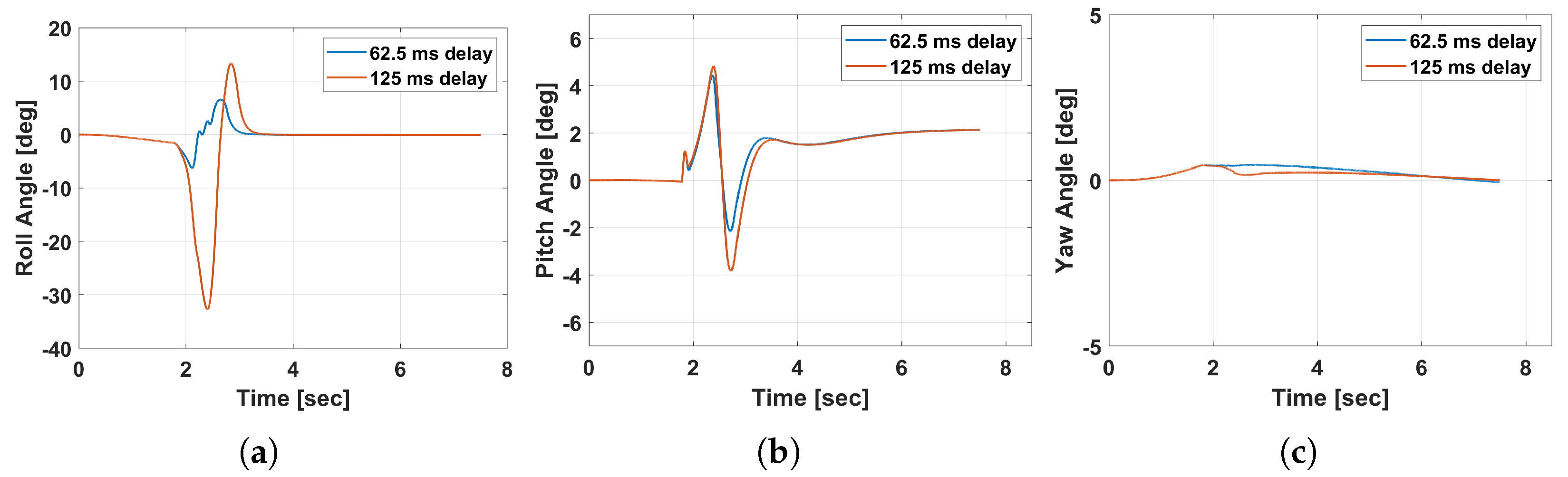
Because roll and yaw are inertially coupled due to the diagonal components in the inertia tensor, a small yaw rate is also induced, which is shown in Figure 18c. Contribution to the induced yaw rate also arises from the differential drag, where the left wing has a higher drag than the right wing. The orientation of the aircraft throughout this maneuver is shown using the Euler angles in Figure 19, where the roll, pitch, and yaw angles are displayed in Figure 19a, Figure 19b, and Figure 19c, respectively. The largest difference between the two scenarios is manifested in the roll Euler angle—the peak roll angle for the 62.5 ms delay case is approximately $-5°$, whereas the peak roll angle for the 125 ms case is approximately $-30°$.

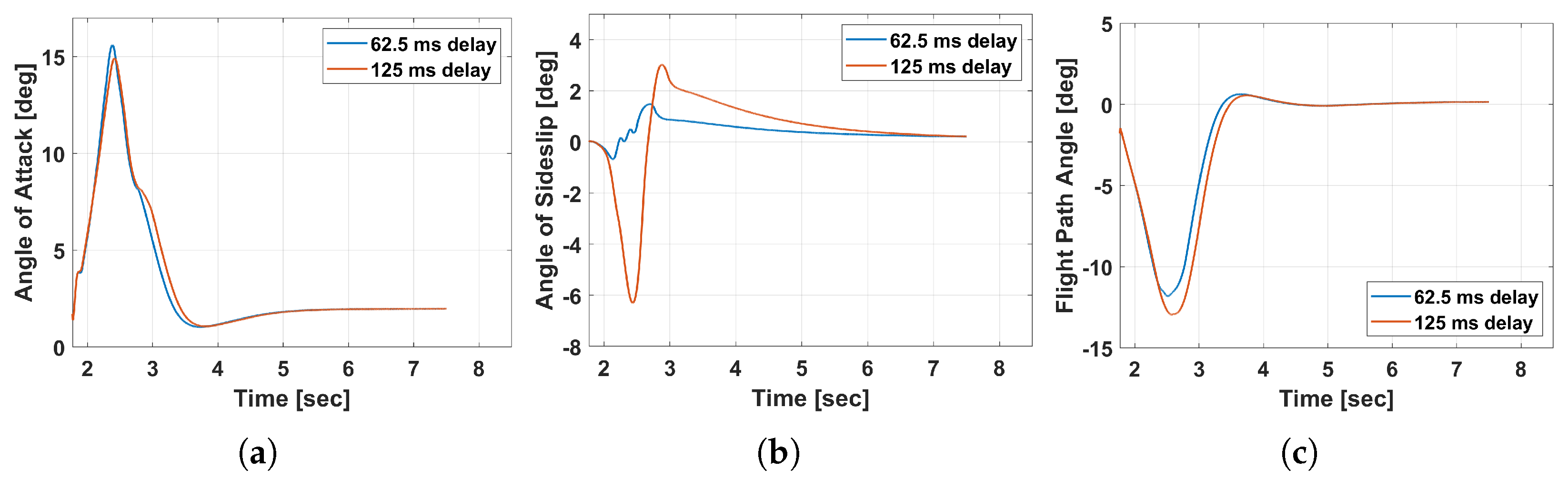
The aerodynamic angles for the asymmetric launch are shown in Figure 20, where the angle of attack (Figure 20a), angle of sideslip (Figure 20b), and flight path angle (Figure 20c) are shown in the subplots. The difference between the angles of attack for each unfolding scenario and the difference between flight path angles for each scenario are quite small relative to the difference in the angles of sideslip; there is considerably more sideslip for the 125 ms scenario. After the wings are unfolded, the flight path angle in Figure 20c shows that the aircraft can successfully fly level regardless of the delay in wing unfolding.

The control surfaces used for the asymmetric launch scenarios include the ailerons, elevator, and rudder, and their respective deflections are shown in Figure 21a, Figure 21b, and Figure 21c, respectively. It should be noted that only the left aileron is plotted here because the right aileron always deflects with an identical magnitude in the opposite direction. These control surfaces are initialized immediately after launch at $t=1.75$ s. Between the two scenarios, the aileron and rudder require very different deflections to stabilize the vehicle. On the other hand, the elevator deflections are almost identical between deployment scenarios. As the left wing deploys first, a negative lift is produced, which results in a negative roll rate. To correct this, the left aileron saturates at ${\delta }_a=20°$, where a positive deflection implies the trailing edge is pointing downwards. The observed saturation is a result of the aileron’s limited effectiveness, as the wings have not yet fully unfolded. In both scenarios, the ailerons saturate; however, the 125 ms case forces the ailerons to saturate for more than double the time of the $62.5$ ms case.

The rudder deflection is shown in Figure 21c, where it can be seen that a negative rudder deflection (trailing edge pointing starboard) results in a positive yawing moment about the ${\widehat{\mathbf{b}}}_3$ axis. For the $62.5$ ms delay scenario, rudder deflection is minimal compared to in the 125 ms scenario, where a large rudder deflection is required to keep the yaw Euler angle of the aircraft close to $0°$. Immediately after launch, a negative rudder deflection is applied to oppose the negative yaw rate shown in Figure 18c.

After the wings are fully deployed ($t=3.5$ s), the vehicle quickly returns to roll and yaw angles of $0°$. Furthermore, it is able to find an elevator deflection of $7°$ to trim the aircraft for $\gamma =0°$, indicating that the aircraft is operating in level horizontal flight.

Animations of the transition maneuver, ground launch, air launch, and air launch with asymmetric wing folding were rendered using Unreal Engine (v 5.3) [32]. Here, the positions, attitude, and control deflections were all prescribed directly from the RCAS output. The link to the video rendering of the transition and ground launch simulations can be found in [33]. In addition, the rendering of the nominal air launch maneuver can be found in [34], and the rendering of the air launch with asymmetric wing unfolding can be found in [35].

5. Summary and Conclusions

The objective of this work was to develop a flight dynamics model for a Tailsitter Air-Launched Uncrewed Aerial System (ALUAS). To model this aircraft, the Rotorcraft Comprehensive Analysis System (RCAS) was used. Using the RCAS, the main components of the Tailsitter were modeled, including the mass/inertia properties, coaxial propellers, thrust-vectoring mechanism, wings and wing folding, and the fuselage aerodynamics, from experimental data. With the model implemented in the RCAS, cascaded PID controllers were designed to control the vehicle’s roll, pitch, and yaw, as well as the flight path angle, by deflecting either the thrust vector or the fixed-wing control surfaces to maneuver the aircraft as desired. RCAS aerodynamic predictions were corrected empirically using the gathered experimental wind tunnel data from a prior study. Simulations with the corrected model included transition between hover and cruise, ground launch, air launch from a moving helicopter, and air launch with asymmetric wing unfolding. The specific conclusions from the study are enumerated below:

1.

Under the current modeling assumptions, the simulations suggest that the Tailsitter ALUAS can perform a large range of complicated maneuvers.

2.

The control effectiveness of the thrust-vectoring gimbal decreases with increasing forward speed, adding motivation to rely on fixed-wing control surfaces such as the elevator.

3.

To perform the transition from hover to cruise, the throttle must be increased enough to avoid large angles of attack, as they could affect performance due to flow separation.

4.

During ground or air launch maneuvers, the aerodynamic effectiveness of the wings varies with their rotation angle during unfolding, which causes large changes in the state variables such as pitch angle.

5.

The delay between the left and right wing unfolding has a huge effect on the overall air launch maneuver; even a small delay can significantly influence the aircraft’s performance and stability. Aileron control must be enabled quickly to ensure minimal divergence.

6. Future Work

Some of the limitations of this work came in the form of modeling assumptions, including (1) neglect of propeller–wing and propeller–fuselage interference, (2) uniform inflow for both propellers, and (3) quasi-steady airloads during wing unfolding. Future work could address these deficiencies by performing a high-fidelity transient CFD simulation of the Tailsitter during launch that includes the propeller wake interaction with the rest of the aircraft. Furthermore, steps will be taken to validate the RCAS flight dynamics model of the Tailsitter by instrumenting the realized vehicle with appropriate sensors to measure the dynamic states. With a time history of the states and control inputs, the RCAS dynamics predictions could be validated for a ballistic launch maneuver. In addition, actuator models should be developed to mimic the specific systems of the realized Tailsitter and then validated.

References

1. Yang, C.; Cai, X.; Wu, L.; Guo, Z. Addressing Launch and Deployment Uncertainties in UAVs with ESO-Based Attitude Control. Drones 2024, 8, 363. [Google Scholar] [CrossRef] [Scilit]
2. Denton, H.; Benedict, M.; Kang, H. Design, development, and flight testing of a tube-launched coaxial-rotor based micro air vehicle. Int. J. Micro Air Veh. 2022, 14. [Google Scholar] [CrossRef] [Scilit]
3. Switchblade. Available online: https://www.avinc.com/lms/switchblade-600 (accessed on 28 February 2024).
4. Anduril Industries: ALTIUS. Available online: https://www.anduril.com/hardware/altius/ (accessed on 16 April 2024).
5. Bouman, A.; Nadan, P.; Anderson, M.; Pastor, D.; Izraelevitz, J.; Burdick, J.; Kennedy, B. Design and Autonomous Stabilization of a Ballistically-Launched Multirotor. In Proceedings of the 2020 IEEE International Conference on Robotics and Automation (ICRA), Paris, France, 31 May–31 August 2020; pp. 8511–8517. [Google Scholar] [CrossRef] [Scilit]
6. Liu, Y.; Du, D.; Zhou, M.; Chang, M.; Hui, Z.; Bai, J. Conception, Design and Flight Testing of a Tube-Launched Jettisonable-Fin Foldable Multirotor. In Proceedings of the 2nd Aerospace Frontiers Conference (AFC 2025); Springer: Singapore, 2026; pp. 624–648. [Google Scholar]
7. Cai, J.; Denton, H.; Benedict, M.; Kang, H. Development of a tube-launched tail-sitter unmanned aerial vehicle. Int. J. Micro Air Veh. 2024, 16. [Google Scholar] [CrossRef] [Scilit]
8. Dooher, J.; Coleman, D.; Benedict, M. A High-Performance Tailsitter Design for Future Air-Launch Capability. In Proceedings of the Vertical Flight Society Forum 81, Virginia Beach, VA, USA, 20–22 May 2025. [Google Scholar]
9. Ott, J.; Biezad, D. Design of a tube-launched UAV. In Proceedings of the AIAA 3rd “Unmanned Unlimited” Technical Conference, Workshop and Exhibit, Chicago, IL, USA, 20–23 September 2004; p. 6493. [Google Scholar]
10. Karatzas, E.; Nikolaou, E.; Pitsis, A.; Alexopoulos, S.; Roussos, S.; Georgantakis, E.; Lappas, V.; Kostopoulos, V. Conceptual design and analysis of a tube-launched fixed-Wing UAV with integrated folding wing systems. Aerosp. Sci. Technol. 2026, 168, 111248. [Google Scholar] [CrossRef] [Scilit]
11. Si, P.; Wu, M.; Huo, Y.; Wu, Z. Investigation of a Tube-Launched Unmanned Aerial Vehicle with a Variable-Sweep Wing. Drones 2024, 8, 474. [Google Scholar] [CrossRef] [Scilit]
12. Gao, L.; Jin, H.; Zhao, J.; Cai, H.; Zhu, Y. Flight Dynamics Modeling and Control of a Novel Catapult Launched Tandem-Wing Micro Aerial Vehicle With Variable Sweep. IEEE Access 2018, 6, 42294–42308. [Google Scholar] [CrossRef] [Scilit]
13. Cheng, H.; Shi, Q.; Wang, H.; Shan, W.; Zeng, T. Flight dynamics modeling and stability analysis of a tube-launched tandem wing aerial vehicle during the deploying process. Proc. Inst. Mech. Eng. Part G J. Aerosp. Eng. 2022, 236, 262–280. [Google Scholar] [CrossRef] [Scilit]
14. Zhang, H.; Yang, Y.; Cai, R. Dynamics simulation of folding wing UAVs launched from a high-altitude balloon platform. Proc. Inst. Mech. Eng. Part G J. Aerosp. Eng. 2023, 237, 3072–3091. [Google Scholar] [CrossRef] [Scilit]
15. Saetti, U.; Arias, P.T.; Baeder, J.D. Flight Dynamics and Control of a Transitioning Quadrotor Biplane Tailsitter. J. Am. Helicopter Soc. 2025, 70, 1–17. [Google Scholar]
16. Coleman, D.; Benedict, M.; Saj, V.; Gadag, A. Investigation of Forward-Flight Roll-Control Enhancement in a Quadrotor Biplane Tailsitter. In Proceedings of the Vertical Flight Society 82nd Annual Forum and Technology Display, West Palm Beach, FL, USA, 5–7 May 2026; pp. 1–16. [Google Scholar]
17. Jun, D.; Cocco, A.; Saetti, U.; Juhasz, O. Flight Dynamics of a Coaxial Compound Helicopter with Rotor-On-Rotor Interactional Aerodynamics. J. Am. Helicopter Soc. 2026, 71, 1–18. [Google Scholar]
18. Bagai, A.; Leishman, J.G. Free-Wake Analysis of Tandem, Tilt-Rotor and Coaxial Rotor Configurations. J. Am. Helicopter Soc. 1996, 41, 196–207. [Google Scholar] [CrossRef] [Scilit]
19. Sugawara, H.; Tanabe, Y. Numerical investigation of rotor/wing aerodynamic interactions at high advance ratios. J. Aircr. 2019, 56, 2285–2298. [Google Scholar] [CrossRef] [Scilit]
20. Elliott, C.; Saj, V.; Denton, H.; Benedict, M. Design and Flight Dynamics of a Hand-Launched Foldable Micro Air Vehicle. Aerospace 2025, 12, 754. [Google Scholar] [CrossRef] [Scilit]
21. Ryseck, P.; Yeo, D.; Hrishikeshavan, V.; Chopra, I. Aerodynamic and mechanical design of a morphing winglet for a quadrotor biplane tail-sitter. In Proceedings of the Vertical Flight Society 8th Autonomous VTOL Symposium, Mesa, AZ, USA, 28 January–1 February 2019; pp. 29–31. [Google Scholar]
22. Stewart, R.W.; Dooher, J.; Benedict, M. Nonlinear Flight Dynamics Modeling of an Air-Launched Tailsitter UAS. In Proceedings of the Vertical Flight Society 80th Annual Forum and Technology Display, Montréal, QC, Canada, 7–9 May 2024. [Google Scholar] [CrossRef] [Scilit]
23. Ballistically Tube-Launched Tailsitter UAS. Available online: https://youtu.be/2WofGANrIwQ (accessed on 15 April 2026).
24. Advanced Rotorcraft Technology. Available online: https://www.flightlab.com/index.html (accessed on 4 March 2024).
25. XFOIL Subsonic Airfoil Development System. Available online: https://web.mit.edu/drela/Public/web/xfoil/ (accessed on 28 February 2024).
26. Winslow, J.; Otsuka, H.; Govindarajan, B.; Chopra, I. Basic understanding of airfoil characteristics at low Reynolds numbers (104–105). J. Aircr. 2018, 55, 1050–1061. [Google Scholar] [CrossRef] [Scilit]
27. XFLR5. Available online: https://www.xflr5.tech/xflr5.html (accessed on 28 February 2024).
28. Saberi, H.; Khoshlahjeh, M.; Ormiston, R.A.; Rutkowski, M.J. Overview of RCAS and application to advanced rotorcraft problems. In Proceedings of the American Helicopter Society 4th Decennial Specialists’ Conference on Aeromechanics, San Francisco, CA, USA, 21–23 January 2004. [Google Scholar]
29. Hasbun, M.; Saberi, H.; Yeo, H. Overview of RCAS Capabilities and Validations for Rotorcraft and eVTOL Applications. In Proceedings of the Vertical Flight Society’s 80th Annual Forum & Technology Display, Montreal, QC, Canada, 7–9 May 2024. [Google Scholar]
30. Nelson, R.C. Flight Stability and Automatic Control; McGraw-Hill Education Private Limited: Chennai, India, 2010. [Google Scholar]
31. Newmark, N.M. A Method of Computation for Structural Dynamics. J. Eng. Mech. Div. 1959, 85, 67–94. [Google Scholar] [CrossRef] [Scilit]
32. Unreal Engine. Available online: https://www.unrealengine.com/en-US (accessed on 28 February 2024).
33. Transition and Ground-Launch Maneuver Videos. Available online: https://youtu.be/FppWq2TJkG8 (accessed on 28 February 2024).
34. Nominal Air Launch Animation. Available online: https://youtu.be/ZuLztRIDd6A (accessed on 15 May 2024).
35. Air Launch Animation with Asymmetric Wing Unfolding. Available online: https://youtu.be/UbceA2reNGE (accessed on 15 May 2024).
Figure 1. Tailsitter ALUAS prototype.
Aerospace 13 00616 g001
Figure 2. Tailsitter ALUAS mission profile.
Aerospace 13 00616 g002
Figure 3. Roll and pitch deflections of the thrust vector.
Aerospace 13 00616 g003
Figure 4. Aerodynamic angles of interest.
Aerospace 13 00616 g004
Figure 5. Wing unfolding (side view).
Aerospace 13 00616 g005
Figure 6. Implementation of the Tailsitter ALUAS in the RCAS.
Aerospace 13 00616 g006
Figure 7. Air launch setup in the RCAS.
Aerospace 13 00616 g007
Figure 8. General control system architecture.
Aerospace 13 00616 g008
Figure 9. Single-propeller experimental setup.
Aerospace 13 00616 g009
Figure 10. Single-propeller thrust and torque in hover.
Aerospace 13 00616 g010
Figure 11. Time response during transition.
Aerospace 13 00616 g011
Figure 12. Time response during ground launch.
Aerospace 13 00616 g012aAerospace 13 00616 g012b
Figure 13. Aerodynamic loads varying with wing principal angle for different α .
Aerospace 13 00616 g013
Figure 14. Time response during air launch.
Aerospace 13 00616 g014aAerospace 13 00616 g014b
Figure 15. Flight path angle during air launch.
Aerospace 13 00616 g015
Figure 16. Wing-folding principal angles during asymmetric launch.
Aerospace 13 00616 g016
Figure 17. Asymmetric launch: inertial velocities.
Aerospace 13 00616 g017
Figure 18. Asymmetric launch: body angular rates.
Aerospace 13 00616 g018
Figure 19. Asymmetric launch: Euler angles.
Aerospace 13 00616 g019
Figure 20. Asymmetric launch: aerodynamic angles.
Aerospace 13 00616 g020
Figure 21. Asymmetric launch: control surface deflections.
Aerospace 13 00616 g021