Space Situational Awareness in Very Low Earth Orbit for Re-Entry Object Monitoring

Abstract

As the number of objects in orbit increases every year, the number of objects re-entering Earth’s atmosphere grows as well. Re-entry path prediction is tricky, as atmospheric modeling lacks accuracy and requires constant monitoring of the object during re-entry. Ground-based sensors face limitations due to the field of view and weather. This paper explores the novel idea of using star trackers in very low Earth orbit to image Resident Space Objects (RSOs) that are on re-entry path and provides a comparison of different star trackers to determine the most effective parameters. A simulation with 1000 Resident Space Objects on re-entry path was performed and detectability analysis was run using AURICAM, SAGITTA, PCO, IDS, and FAI sensors placed in orbit between 200 and 600 km in altitude. The results show that all star trackers at any altitude were capable of detecting at least three RSOs on re-entry path and making at least 47 detections during the simulation period. In particular, instruments with larger aperture diameters such as SAGITTA and FAI and quantum efficiency performed better, making up to 134 detections and detecting up to 10 unique RSOs. They also detected a higher average signal-to-noise ratio. Detectability of RSOs is higher when the sensor is placed closer to the objects, with the most effective performance recorded at 300–400 km altitude. Future work should include practical testing of this technique.

1. Introduction

Space Domain Awareness (SDA), defined as the capability to detect, track, identify, and characterize space objects and the space environment [1], is increasingly recognized as a critical challenge for space systems for safety, security, and sustainability. SDA is considered an integration of space surveillance and tracking (SST), space weather and space intelligence [2].

For SST, operating in a congested, contested, and competitive space environment (referred to as the three Cs) has never been more challenging in the history of space exploration. Consequently, space situational awareness (SSA—key subset of SDA capabilities), which involves monitoring and characterizing space objects, has been identified by the research community as a top priority for space activities in Canada and worldwide [1]. Damage to space systems has a significant and immediate impact on technologies that we all rely on daily, including navigation, communication, resource management, climate monitoring, and weather forecasting. Space intelligence refers to a wide range of activities that include collecting and processing SDA data and information to identify and characterize space objects through astronomical and photometric analysis [3]. In this study, we focus on information on re-entry objects to estimate and forecast the likely impact of space objects re-entering Earth’s atmosphere, which may pose risks to human safety and critical infrastructure on the surface.

1.1. Re-Entry Events

In 2024, over 2000 objects re-entered Earth’s atmosphere [4]. Several organizations, both governmental and commercial, actively monitor re-entry events and provide information for public awareness. These groups maintain up-to-date databases compiled from observations made worldwide, detailing the type of re-entry, expected dates, and times, along with the last known sightings. For instance, the CORDS Re-entry Database records space objects and payloads that have re-entered Earth’s atmosphere since 2000, offering valuable historical insights [5]. The European Space Agency (ESA), leveraging a data-sharing agreement with the US Strategic Command, incorporates conjunction data messages provided by the US Combined Space Operations Center (CSpOC) alongside its own orbital data [6]. Since 2009, ESA has also been developing software, technologies and precursor systems to test a fully European network that would provide independent data on the risks from spaceflight. Websites like SATVIEW provide real-time tracking and forecasting of space junk re-entry for free to the public [7].

In recent years, the potential threat of re-entry events has also been carefully studied. During re-entry, objects will fragment into smaller pieces at around 85–75 km in altitude [8]. Most of these pieces will burn up in the atmosphere. However, if any surviving parts were to land in populated regions of the Earth’s surface, the casualty risks could be non-negligible. Re-entry predictions for natural re-entries are very difficult and are affected by various sources of uncertainty, particularly in the atmospheric model [9], so ensuring safety on the ground is difficult. In [10], Pardini and Anselmo analyzed objects that re-entered between 2010 and 2022, and found the probability of injuring or killing at least one person to be around 18%. Among the most concerning statistics, the total mass returned from orbital stages increased by approximately 77% in 2022, as a result of the intensification of space activities. The steady increase in the number of re-entry events since 2020 is primarily attributed to the disposal of satellites from the Starlink constellation [10].

Re-entry events also pose potential threats to the aviation industry. In 2003, when the Columbia Space Shuttle exploded, at least nine aircraft flew through the debris field with no knowledge of the threat. Investigation after the event revealed that the chances of being struck with debris ranged from 0.3% to 10% [11]. In 2022, the re-entry of a Long March 5B rocket forced the closure of airspace over Europe, delaying 645 flights. The authors of [12] found a 0.8% chance for high-traffic regions around airports to be affected by uncontrolled re-entries, with the rate rising to 26% for larger but less busy areas around big cities. Precautions must be taken to avoid possible tragedy, but these precautions also cannot repeatedly result in significant inconvenience [13].

Although significant efforts are devoted to monitoring, predicting, and sharing information about re-entry events, the technology used to capture and characterize these events relies predominantly on ground-based observations. These systems, including radar installations such as TIRA [14], optical telescopes such as OWL_Net [15], and radio tracking facilities, provide valuable data on re-entering objects. However, their capabilities are often limited by factors such as weather conditions, line-of-sight constraints, and the resolution of the equipment. Ref. [16] states that observing an object just prior to its re-entry event with an optical telescope is difficult, as most objects have high angular velocities prior to re-entry, which results in short effective exposure times. Ground-based observation windows for low-orbit objects from a single location are also very short. Expanding the ability to image and characterize re-entry events through advanced technologies, such as space-based sensors [17,18] or high-altitude platforms [19,20,21], could greatly enhance the accuracy and comprehensiveness of data collection.

1.2. Predicting Re-Entries

Once space objects are detected, either by ground-based or space-based sensors, their trajectories are estimated using a combination of re-entry and fragmentation analyses. These processes are critical for accurately evaluating the potential threats posed by the objects as they re-enter Earth’s atmosphere. Re-entry analysis involves predicting the path an object will take as it descends, while fragmentation analysis assesses how the object may break apart due to aerodynamic forces and thermal stresses. Together, these analyses provide information on the likely impact zones and the potential hazards to people and infrastructure. Re-entry analysis is typically performed using simulation software.

Previously, ref. [16] used optical observations of LEO satellites to perform orbit determination, which is in turn used to predict the re-entry epoch. The results were compared to predictions made using historical TLE format data from Space-Track, which were also obtained from observations. They found that by enriching the TLE catalog with more observations, the ballistic coefficient could be determined more precisely, leading to more accurate re-entry predictions. Ref. [22] explored the re-entry survivability and ground risk estimations of space debris using an object-oriented re-entry analysis tool. The results were compared with validated simulation tools, Object Re-entry Survival Analysis Tool (ORSAT) [23] and SpaceCraft Atmospheric and Aerothermal Break-up (SCARAB) [24], and the authors found discrepancies in flow properties and heat flux calculations. They also found that as the break-up altitude increased, so did the difference in the impact footprint. Break-up altitude is generally between 85 and 120 km and is loosely defined as the altitude where a space object re-enters Earth’s atmosphere.

The Semi-Analytical Tool for End of Life Analysis (STELA) is a reference tool developed by CNES for long-term orbit propagation to determine whether objects are compliant with the French Space Operations Act, ensuring that non-operational objects are removed from orbit. STELA is also used as part of early warning and crisis management systems [25]. STELA only takes into account the perturbations that have a significant effect in the long term, where long-time-scale analyses are based on numerical integration of equations of motion. Short-period terms are removed by analytical averaging for conservative perturbations and numerical averaging for dissipative perturbations [26]. This allows STELA to have very large timesteps, even 24 h, and to propagate a model for hundreds of years. STELA was used in this research to propagate the orbital paths for the example RSOs. More information on STELA can be found in [25].

The limitations of these prediction methods come from their lack of ability to handle the uncertainty associated with re-entry. Aerodynamic forces heavily influence the re-entry path and cannot be simulated with very high accuracy. An RSO’s future trajectory will be heavily influenced by strong perturbations such as Earth’s J2 effect and atmospheric drag, which continuously alter the orbits over time. As an object nears re-entry, the drag force becomes dominant, causing rapid orbital decay. The highly dynamic and unpredictable variations in an object’s shape, mass distribution, material, structural integrity, and thermal properties also contribute to the difficulty level. Therefore, any effort to assist in providing better accuracy in the prediction of landfall (location, time and potential impact) would significantly improve preparation. Previous studies have shown that additional observations during orbital decay can improve re-entry prediction workflows. In Ref. [27], the authors find that frequent measurements and eliminating tracking gaps between 100 km and 50 km altitude are key to reducing the inaccuracy of estimations. Space-based sensors in very low Earth orbit could partially fill in that gap. Ref. [28] states that higher frequency of observations leads to more accurate determination of the behavior of the drag coefficient, especially at low altitudes where uncertainties are large. Ref. [29] found that combining re-entry data from multiple sources improves re-entry predictions and reduces associated uncertainties. Using space-based sensors to capture RSOs before they re-enter can contribute to the pool of orbital data available, improving re-entry trajectory and epoch prediction.

In this study, we look at the feasibility of monitoring objects in very low Earth orbit (VLEO) that will re-enter Earth’s atmosphere within the next few weeks or months, using space-based optical sensors. We also provide a comparison between five different sensors and determine which parameters have the most significant effect on performance. Ref. [30] performs a detectability analysis of wide-field-of-view sensors on co-orbital RSOs by using distance and visual magnitude to calculate the signal-to-noise ratio. A similar method is used in this study, adjusted to specifically track re-entering RSOs. The proposed observation approach begins imaging in VLEO (400–200 km) as RSOs start the descent phase, but before the object reaches the re-entry point (120 km) above the break-up altitude (85 km). The host sensor was placed between 200 and 600 km in altitude, targeting RSOs in orbit between 200 and 400 km in altitude. Simulations were run with 1000 RSOs and one of five star trackers over a 30-day period.

This study finds that it is possible to use commercial wide-field-of-view star trackers in VLEO to detect re-entering RSOs. A higher aperture diameter and quantum efficiency have significant impacts on an instrument’s performance. The distance between the observed objects and the sensor is found to influence detectability, and as a result, the 300–400 km altitude range proved to be the richest environment for re-entry object detection, as it is the most heavily populated region in VLEO. Many re-entering RSOs were detected repeatedly, some up to 34 times during the month-long period. These detections would be ideal for enriching the existing pool of observation data to improve re-entry predictions.

Section 2 covers the setup of the simulation, detailing the initial parameters and mathematics. Section 3 discusses the results of the simulation as well as the limitations of the experiment. Section 4 summarizes the work and looks briefly at the next steps.

2. Materials and Methods

2.1. Study Parameters

The host observer’s orbit was placed between 200 and 600 km in altitude. The orbital parameters of the host satellite are listed in Table 1, pulling from previously retrieved Two-Line Elements (TLEs) for the International Space Station (ISS) from 20 February 2026. The ISS TLE was used only as a representative low-Earth-orbit case characterized by rapid orbital motion, rather than to model the ISS itself. The altitude is varied to explore where the most effective orbit would be for the host sensor.

Table 1. Host and target orbital parameters.

Orbit Element	Host Orbit
Orbit Altitude	200–600 km
Eccentricity	7.4760 × 10−4
Inclination	51.6°
RAAN	124.1°
Argument of Perigee	354.2197°
Mean Anomaly	178.2°

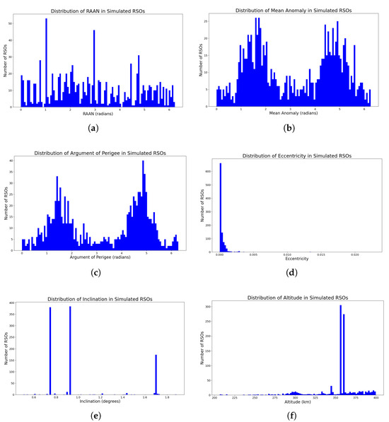
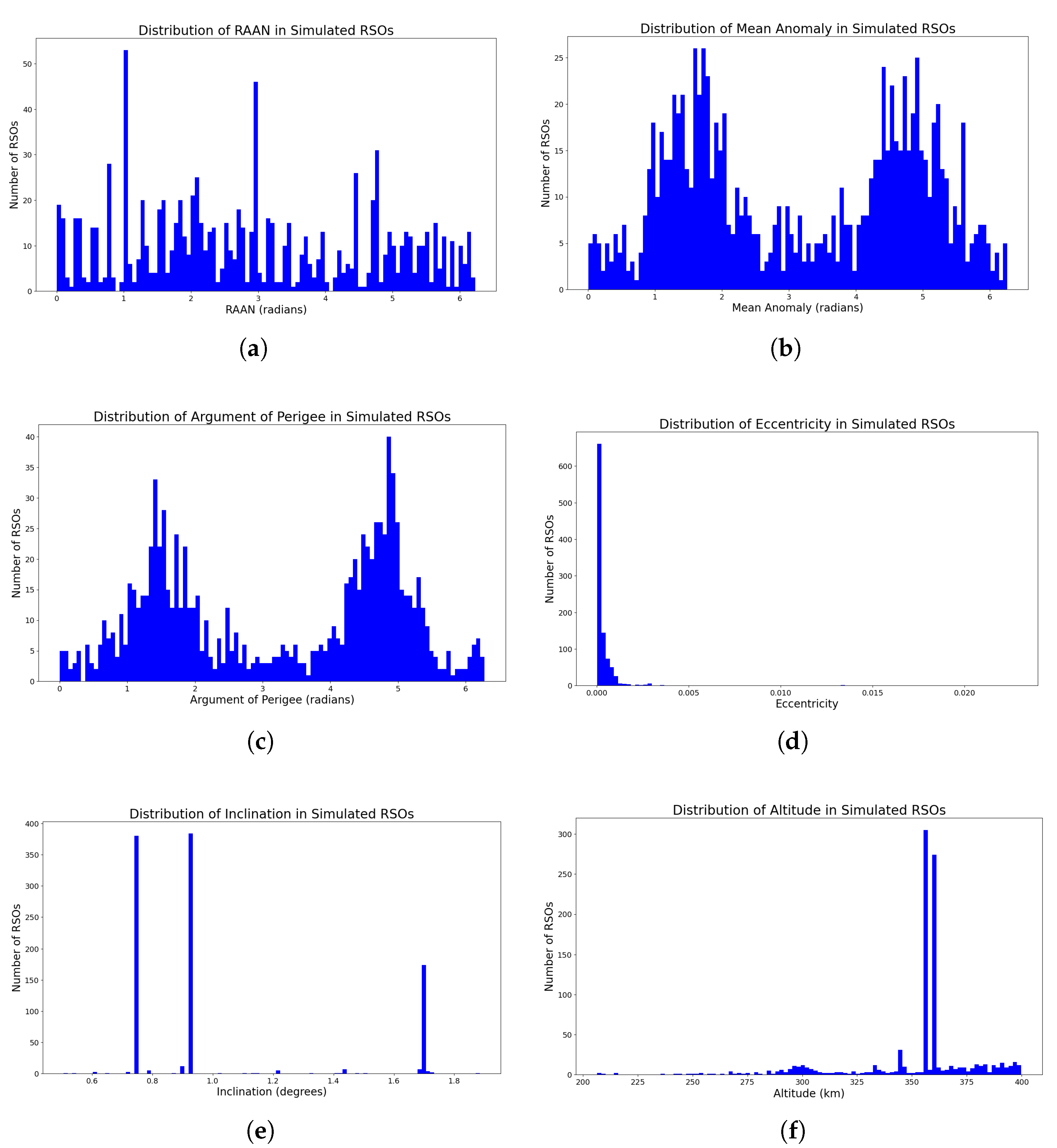
One thousand RSOs located between 200 km and 400 km in altitude on re-entry paths were simulated. The orbital paths of these RSOs were modeled using orbital parameters retrieved from TLEs obtained from Space-Track. These TLEs were arbitrarily chosen from the population of recently re-entered objects to be representative of the larger RSO population in VLEO. The distribution of their parameters is shown in Figure 1. The diameters and masses of each object were retrieved from ESS’s DISCOS catalog using API requests. If either of these values was not available, a placeholder value of 0.2 m was used for the diameter, as this is on the lower end of the size of RSOs we are tracking and would adequately test the limits of the sensor. A mass of 250 kg was used, as this was the average of the retrieved values. The distribution of the other orbital parameters amongst these propagated RSOs is shown in Figure 1. A signal-to-noise ratio (SNR) limit of 6 was chosen to ensure true detection. A distance limit from the host to the RSO of 550 km was chosen to ensure that the target RSO would not be occluded by the Earth. The solar phase angle limit of less than 90° was chosen to ensure sufficient illumination of the object for detection by the host sensor.

Figure 1. Distribution of orbital parameters for the propagated RSOs. RSOs were chosen at random from Space-Track. (a) Distribution of RAAN in propagated RSOs. (b) Distribution of mean anomaly in propagated RSOs. (c) Distribution of argument of perigee in propagated RSOs. (d) Distribution of eccentricity in propagated RSOs. (e) Distribution of inclination in propagated RSOs. (f) Distribution of altitude in propagated RSOs.

The RSOs were propagated for 30 days in STELA. This duration was chosen because objects in the 200 km to 400 km altitude range can take about a month or more to re-enter. Break-up altitude was set at 85 km [31], below which the simulation was ended to save computation time. These parameters are summarized in Table 2. The host orbit does not decay and was modeled separately, as it is assumed that there will be maintenance during the mission.

Table 2. Detectability analysis parameters.

Analysis Parameter	Value
Orbit Propagation Duration	30 days
Timestep	1 min
Number of RSOs	1000
Minimum SNR	6
Solar Phase Angle	<90°
Maximum Distance	550 km

The sensors used in the detectability study are the Fast Auroral Imager (FAI), the UI-3370CP-M-GL IDS camera, the PCO Panda 4.2 camera, the AURICAM and the SAGITTA sensor. FAI is a dual charge-coupled device/single-controller camera that is used to image auroral emissions in the 630–1100 nm wavelength range and is currently aboard Cascade, Smallsat and Ionospheric Polar Explorer (CASSIOPE) [30]. FAI has also previously been used to detect and track RSOs from orbit [17,18]. The IDS and PCO cameras were both used to capture starfield images during a stratospheric balloon mission [21]. The AURICAM is based on technology derived from the Auriga star tracker heads and has been flight-tested since 2019. Finally, the SAGITTA is a flight-tested Cubesat-compatible star tracker. These sensors were selected because they have previously been applied in SSA studies, and most of their relevant sensor parameters are publicly accessible. Their parameters are listed in Table 3.

Table 3. Parameters for all the sensors used in this feasibility study. Pixel pitch is the distance between the center of two pixels. FOV is the acronym for field of view, which is the angle that is visible within the observation frame. Focal length refers to the distance between the center of the lens and the point of its focus. QE is quantum efficiency, which measures how efficiently a device converts photons into useful output. Aperture diameter is the physical size of the lens. The 5 instruments looked at in this study are the AURICAM [32], the SAGITTA [33], the PCO [34], the IDS [35], and the FAI [36].

	AURICAM	SAGITTA	PCO	IDS	FAI
Pixel pitch (µm)	5.5	5.5	6.5	5.5	26
Focal length (mm)	10	25	25	16.5	13.8
QE (percentage)	95	66	78	50	66
Aperture diameter (cm)	0.25	1.725	1.25	1.6	1.725
Field of view (degrees)	35 × 35	25.4 × 25.4	29.6 × 29.6	41 × 41	26 × 26

The position of each RSO at each timestep was compared to the position of the sensor to find their solar phase angle and the distance between them. The SNR registered by the instrument from the RSO was then calculated. Anytime the SNR exceeded 6 was considered a detection. An instrument can detect multiple RSOs simultaneously, as a detection simply indicates that the sensor was able to capture an image where the RSO was visible.

2.2. Calculations

The orbit of the host object is assumed to maintain the same altitude throughout. Therefore, it is simply a matter of moving the object around the established orbit over time. At each step, the orbital rate is calculated based on the semi-major axis and then used to calculate how much the object has moved along a flat orbit. Then, the argument of perigee, inclination and longitude of ascending are taken into account to find the position of the object along its real orbit. A better explanation of the mathematics can be found in [30].

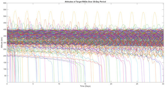
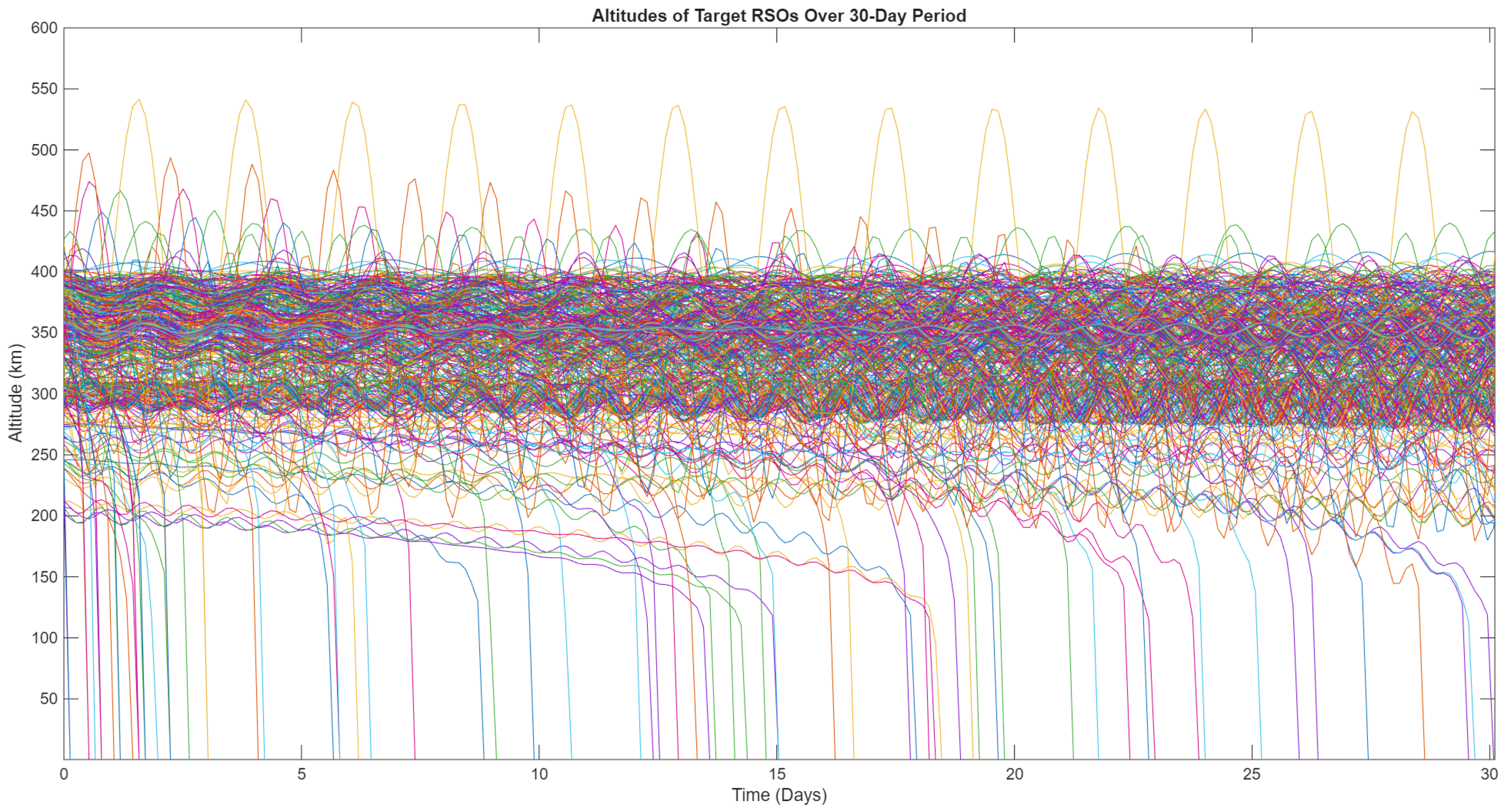
STELA was used to calculate the Earth-centric position of 1000 different RSOs, from the position indicated by the TLE until the moment of re-entry, where the RSO reaches break-up altitude. The altitudes of all 1000 RSOs are plotted in Figure 2. The STELA integrator takes into account Earth’s gravity field, solar and lunar gravity, atmospheric drag, solar radiation pressure, and solid tides [26]. The default integrator used is a sixth-order Runge–Kutta. All RSOs were integrated using the LEO dynamical model. The TLEs are initially converted to osculating orbit parameters using the SGP4 propagator. The osculating orbit refers to the real state vector of the spacecraft at a given date and takes into account short-term perturbations. More details about STELA and its propagation models can be found in the STELA User Manual [26] available on the CNES website.

Figure 2. Altitude of all 1000 RSOs simulated over the month-long period, each RSO is represented with a different coloured line; 7.2% of the simulated objects re-entered during this time.

At each timestep, the solar phase angle between the RSO and the host is evaluated using Equation (1).

$$\Phi =\pi -|co{s}^{-1}[(TargetPositio{n}_{ECI}-HostPositio{n}_{ECI})·SunECI]|$$

(1)

This is calculated by taking the dot product of the target position as measured from the host sensor’s Earth-centred inertial (ECI) frame and the Sun’s ECI position. $TargetPositio{n}_{ECI}$ refers to the target’s position in the Earth-centred inertial frame, and $HostPositio{n}_{ECI}$ refers to the host’s position in the Earth-centred inertial frame.

Equation (2) relates illumination phase angle to the fraction of light reflected.

$$F(\Phi )=({\displaystyle \frac{2}{3{\pi }^2}})[(\pi -\Phi )cos\Phi +sin\Phi ]$$

(2)

The RSOs are modeled as spheres for simplicity.

Equation (3) calculates the visual magnitude of the target in reference to the visual magnitude of the Sun.

$$m_{v,obj}=m_{v,sun}-2.5log({\displaystyle \frac{\rho AF(\Phi )}{R^2}})$$

(3)

$\rho$ is the target RSO’s reflectivity, which is set at 0.2 in this simulation, A is the area of the target, and R is the distance between the target and the RSO.

Equation (4) calculates the photon irradiance.

$$E_{RSO}=5.6\times {10}^{10}\times {10}^{-0.4m_{v,obj}}$$

(4)

In Equation (5), the number of signal photoelectrons is calculated.

$$e_s=QE\times \tau \times A_{aperture}\times E_{rso}\times t_{signal}$$

(5)

$QE$ is the sensor’s quantum efficiency, $\tau$ is the optical transmittance, $A_{aperture}$ is the area of the aperture, and $t_{signal}$ is the signal integration time. This is calculated using Equations (6) and (7). Equation (6) calculates the instantaneous field of view.

$${\theta }_{pixel}={\displaystyle \frac{PixelPitch}{FocalLength}}$$

(6)

$$t_{signal}=minimum({\displaystyle \frac{{\theta }_{pixel}}{\omega }},t_{int})$$

(7)

In Equation (7), $\omega$ is the angular rate of the target and $t_{int}$ is the sensor integration time.

The background noise is calculated using Equations (8) and (9).

$$L_b=5.6\times {10}^{10}\times {10}^{-0.4M_b}\times {(\frac{180}{\pi })}^2\times {3600}^2$$

(8)

$$e_b=QE\times \tau \times L_b\times A_{aperture}\times {\theta }_{pixel}^2\times t_{int}$$

(9)

$L_b$ is the background signature, and $M_b$ is the background visual magnitude per square arcsec and is set to 20. $e_b$ is the number of background photoelectrons.

Finally, SNR is calculated using Equation (10).

$$SNR={\displaystyle \frac{e_s}{\sqrt{e_b+e_n^2+(e_{DC}\times t_{int})}}}$$

(10)

$e_n$ is the read noise, and $e_{DC}$ is the dark current noise.

Additional details about these equations can be found in [30]. The number of occasions where the distance, the SNR and the solar phase angle all satisfy the detectability parameters laid out in Table 2 was tabulated.

3. Results

The results for a sensor placed at 200 km altitude are shown in Table 4. SAGITTA had the most detections in comparison to all instruments. FAI, PCO and IDS all performed similarly, while AURICAM made fewer detections. At 300 km altitude, SAGITTA once again had the best performance. FAI, PCO, and IDS again all performed similarly, with slightly fewer detections. This trend continues through 400 and 500 km, with SAGITTA continuing to perform the most effectively. FAI continues to be slightly more effective than PCO, which is slightly more effective than IDS at each of these altitudes. At 600 km, all the instruments aside from AURICAM were able to make the same number of detections. AURICAM consistently registered fewer detections than the other instruments. These results are consistent with the relative sizes of each instrument’s aperture diameter.

Table 4. Number of total detections, number of unique RSOs detectable, average signal-to-noise ratio of detections, average duration of detections, and average distance between the sensor and the detected object when sensors are placed at different altitudes.

Altitude (km)	Instruments
		FAI	PCO	IDS	SAGITTA	AURICAM
200	Total Detections:	96	95	92	99	67
	Number of RSOs Detected:	5	5	5	6	4
	Average SNR:	82.4	73.9	65.2	88.9	17.8
	Average Detection Duration (timesteps):	1.76	1.77	1.79	1.74	1.31
	Average Distance to Object (km):	381.9	383.0	386.3	378.9	303.7
300	Total Detections:	128	120	116	131	73
	Number of RSOs Detected:	10	9	8	10	4
	Average SNR:	87.0	80.7	71.3	94.2	21.0
	Average Detection Length (timesteps):	1.59	1.63	1.65	1.57	1.33
	Average Distance to Object (km):	340.9	347.1	351.1	339.3	297.3
400	Total Detections:	131	128	119	134	72
	Number of RSOs Detected:	9	9	9	10	4
	Average SNR:	89.1	80.7	76.6	92.4	21.6
	Average Detection Length (timesteps):	1.50	1.52	1.55	1.49	1.32
	Average Distance to Object (km):	336.6	338.9	357.0	324.8	305.5
500	Total Detections:	108	104	100	114	68
	Number of RSOs Detected:	6	6	6	6	4
	Average SNR:	58.6	53.5	47.4	62.3	12.3
	Average Detection Length (timesteps):	1.56	1.59	1.61	1.54	1.25
	Average Distance to Object (km):	383.3	387.4	391.7	378.1	338.8
600	Total Detections:	79	79	79	79	47
	Number of RSOs Detected:	4	4	4	4	3
	Average SNR:	47.6	42.7	37.0	52.4	9.22
	Average Detection Length (timesteps):	1.56	1.56	1.56	1.56	1.15
	Average Distance to Object (km):	433.3	434.3	433.8	433.8	364.7
	Total Detections Across All Altitudes	542	526	506	557	327

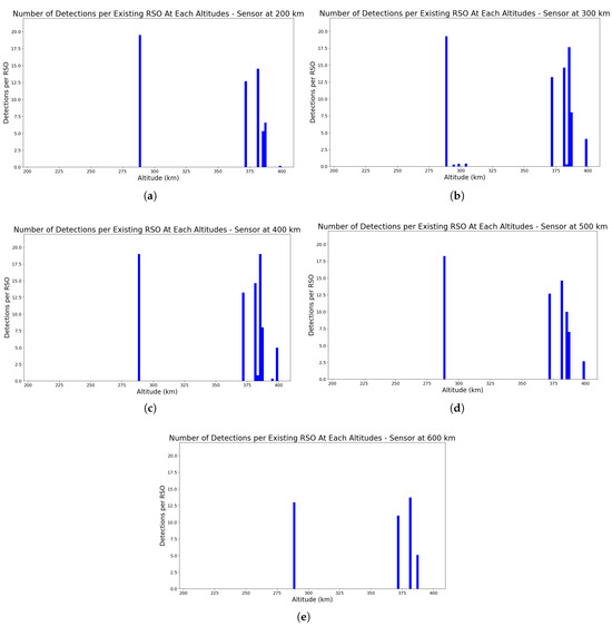
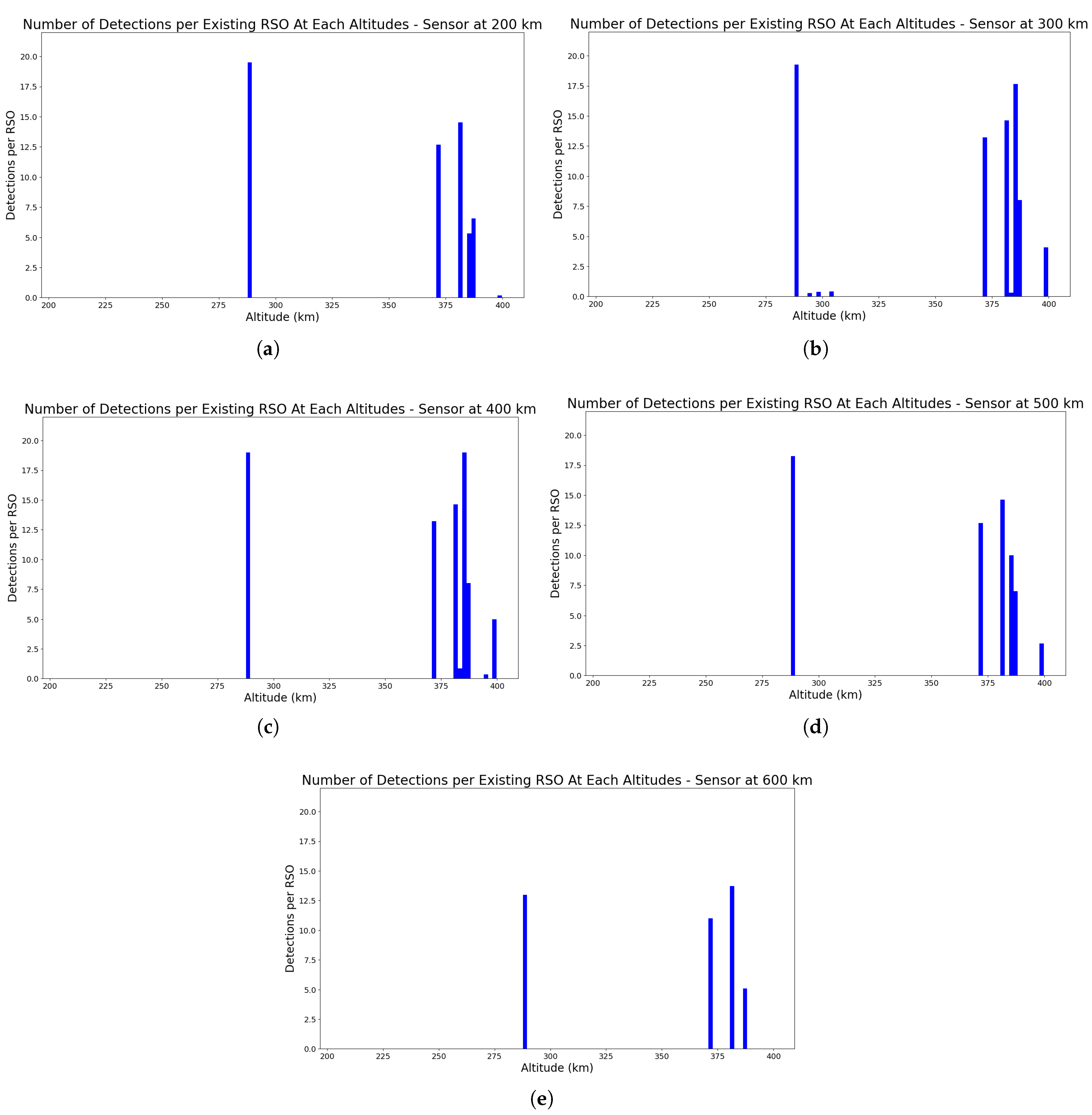
The largest number of detections occurred at altitudes of 300 and 400 km for all instruments. The average SNR is also highest for all instruments in this range. This is unsurprising, as looking at Figure 1f, the majority of the RSOs simulated are within that range. The average detected objects are about 30 to 50 km closer to the instrument than at 200 km and 500 km. The distance between the object and the instrument plays an important role in detectability. The instruments perform better when they are placed close to as many of the orbiting objects as possible. To remove any bias due to the uneven distribution of initial conditions in the simulated objects, the number of detections of objects in each altitude bin in Figure 1f was divided by the total number of simulated objects within that bin. The results at each altitude are shown in Figure 3; 300 and 400 km have a less dramatic advantage when the data is processed this way, but placing the sensor at 300 and 400 km altitude still provides the best results overall.

Figure 3. Number of detections of objects in each bin divided by the number of objects in each bin. (a) Results with the sensor at 200 km altitude. (b) Results with the sensor at 300 km altitude. (c) Results with the sensor at 400 km altitude. (d) Results with the sensor at 500 km altitude. (e) Results with the sensor at 600 km altitude.

A more detailed breakdown of the results revealed that many of the RSOs were detected repeatedly. There were a few RSOs at altitudes 300 and 400 km that were detected once during the entire month, and those RSOs generally were not detected at other altitudes. At 200 km, RSO #912 was detected only once by IDS, but multiple times by other instruments. For other RSOs, the number of repeated detections ranged from 2 times to 34 times. These RSOs were often detectable at multiple altitudes. For example, the four RSOs detected at the 600 km altitude (#407, #447, #524, and #834) were detected by all instruments besides the AURICAM for the same number of detections. Even the length of each detection was the same at that particular altitude. These particular objects were also detected at every altitude by multiple instruments. RSO #324 and #912 were both detected from 200 to 500 km altitude, each time by multiple instruments, for a repeated number of times. Comparing the parameters for these RSOs reveals that they are all larger objects. Their masses range from 960 kg to 3800 kg, and their diameters range from 1.69 m to 10.89 m. These six RSOs made up the majority of the detections for all instruments across all altitudes. Some smaller objects were also detected, but only at 300 or 400 km altitude, and only once or twice over the 30-day period.

The length of each detection ranged from 1 timestep to 3 timesteps, with each timestep being 60 s. The average detection duration was longest at 200 km altitude and pretty similar at all other altitudes. At 600 km altitude, 0 detections out of the 79 made exceeded 2 timesteps for all instruments. The IDS camera had the longest average durations for the detections it was able to make.

The signal-to-noise ratio for detections ranges from 6.0 to 2485.4, but is between 50 and 100 on average. From Table 4, it is obvious that the AURICAM consistently registers significantly lower SNRs than the rest of the instruments, while SAGITTA records higher SNRs. This again is likely due to the higher aperture diameter. The solar phase angles for all detections range from 1.165 radians up to the cutoff angle, suggesting that it may be possible to detect RSOs even beyond the 90-degree phase angle.

From these results, we can see that it is possible to detect RSOs on re-entry paths using a camera in orbit, although the detections will be very brief for each object, and only a small fraction of the total RSOs will be detectable. This method will mostly be suited for more massive objects with larger diameters. All instruments were capable of making detections, but sensors with larger aperture diameters were shown to be more effective. This is because a larger aperture diameter enables more light to be captured by the instrument, resulting in a larger signal [37]. At the same time, a larger aperture results in a shallower depth of field, but this is offset by the shorter focal length, which results in a wider depth of field [38]. A higher quantum efficiency indicates a more sensitive sensor, which also results in a more effective performance from the instrument. SAGITTA and FAI were simulated to have the same aperture diameter and quantum efficiency, but SAGITTA performs slightly better consistently. From Equation (6), it is clear that the ratio of the pixel pitch to the focal length also plays a factor. The pixel pitch should be larger to improve the signal-to-noise ratio. However, if the focal length is too small, this results in less details per pixel [39]. Therefore, the ratio of pixel pitch to focal length must be small to ensure sufficient information in each pixel of captured images. The 300 and 400 km altitudes are the best orbits to place the instrument, as these altitudes return the largest number of detections, even when the data is normalized by the number of objects at that altitude.

Limitations

This simulation does not account for the pointing direction of the sensors or finite FOV. Only the phase angle between the sun and the detector is calculated using ECI vectors of the positions of both objects. Therefore, the true number of detectable RSOs may be less, as some objects will approach the sensor outside its field of view. This study also omits Earth shadow, Sun/Moon exclusion angles, slewing constraints and other variables as it is only a preliminary feasibility study. Future work would include these operational constraints to determine how these factors reduce the number of detection opportunities.

On the other hand, the 1000 RSOs simulated are only a fraction of the number of RSOs actually found in VLEO. This will increase the number of detectable approaches. The diameter of each object is also either retrieved from the online database or simply set as 0.2 m. The diameter affects the object’s magnitude as well as its re-entry path, so inaccurate data will affect the model. The mass is also retrieved in the same way, and a default value of 250 kg is assigned if none is available. The mass is used in calculating the re-entry path and, therefore, also impacts the realism of the model. From the results, it is clear that more massive objects with larger diameters are detected more easily.

The population of RSOs simulated was chosen at random from the TLEs of existing re-entering debris, but there are significantly more RSOs in the 300 to 350 km altitude range, as seen in Figure 1f. A total of 911 of the 1000 RSOs are located between 300 km and 400 km. This inevitably skews the results to favor placing the host closer to that altitude range, even with any attempts to normalize the data. However, as this data is pulled from recent decaying objects on Space-Track, we believe that this is reflective of the existing RSO population in VLEO.

Some camera parameters, such as dark current, readout noise and optical transmittance, were not available for all sensors. Therefore, the values for FAI were used for dark current and optical transmittance, and the value for PCO was used for readout noise when respective parameter data were unavailable. The aperture diameter and quantum efficiency were also unavailable for SAGITTA, so values were estimated based on other sensors. Since aperture diameter appears to influence the results, the choice of value for SAGITTA’s aperture diameter makes the instrument appear more effective. The conclusion, then, should not be that SAGITTA is necessarily the best-suited instrument, but rather that a wider aperture diameter is needed for this task.

This research assumes a visual magnitude of 20 for the sky in calculating background noise, with no adjustments for when the Earth is in the background of the image, which will increase the noise significantly due to reflected light from the Sun. The visual magnitude of the Earth changes depending on whether the Earth is in a crescent or full. It is also possible that if the star trackers are imaging co-orbital objects, the Earth has less of an effect on the SNR. Either way, the SNR calculations will have to be adjusted to accommodate. However, given that the average SNR detected for the majority of the instruments far exceeds the minimum criteria of 6, object detection should still be possible even with additional noise from the Earth.

STELA uses the semi-analytical approach and is therefore generally used for long-term integrations. The major benefit of STELA is its ability to run relatively accurate simulations lasting 100 years in shorter amounts of time by using large integration steps. STELA achieves this by ignoring short-term perturbations to save computation time without losing precision. Even for shorter-term propagation, the expected integration timestep is expected to be in the order of an hour. This project uses integration steps of one minute. Therefore, the precise position and velocity of each RSO at each timestep may not be accurate. However, the purpose of propagating RSO orbits in this research was not to exactly predict their re-entry path, but rather to simulate the presence of re-entering objects that could be imaged. Therefore, for the intended purpose of this paper, the re-entry paths calculated by STELA should suffice.

4. Conclusions

RSOs were simulated in VLEO using STELA with a host sensor placed in orbit at altitudes between 200 and 600 km to determine the detectability of RSOs on a re-entry path using a PCO, FAI, IDS, AURICAM or SAGITTA camera in VLEO. The results showed that all tested star trackers were capable of detecting re-entering RSOs, while instruments with larger aperture diameters were able to detect more re-entering objects. The distance between the instrument and the RSOs is an important factor, as the sensors are more effective at capturing the RSOs closer to their orbit. With a large portion of the RSOs simulated being in the 300 to 400 altitude range, this was also the best range for the sensor to orbit to achieve the best performance.

Instruments were able to detect up to 10 individual RSOs over a month-long period. Some RSOs were detected up to 34 times. The length of the detection never exceeded three timesteps, which is a time period of two minutes. The IDS camera had the highest average detection length for the detections.

This method appears effective at imaging more massive RSOs with larger diameters. The most often detected objects have diameters exceeding 1.5 m. Smaller RSOs are still detectable, but at a much lower frequency. However, the 1000 RSOs are only a small fraction of the real RSO population, and a larger number of objects would provide a much richer environment for RSO detection.

One of the detection criteria chosen is a solar phase angle of less than 90 degrees. This was to ensure sufficient illumination of the object by the Sun for the instrument to capture. However, it is very possible for the instrument to detect objects with a phase angle exceeding 90 degrees as long as the SNR is still 6 or above. When the detection analysis was conducted without the solar phase angle requirement while the other criteria were maintained, the number of detections and the number of RSOs detected increased at every altitude and across every instrument. The overall trends remained the same.

The detections shown here would provide orbital information about re-entering RSOs in the weeks or months leading up to re-entry. By themselves, they may or may not be sufficient to generate precise re-entry epoch or accurate path predictions, but combined with observations from ground sources, on-board GPS [28] or other space-based sensors, they can improve the accuracy of orbit determination and re-entry models, and decrease uncertainties [29]. Space-based sensors also have the unique benefit of providing continuous coverage regardless of weather conditions.

Future work would include additional simulation work considering constraints that were assumed or ignored in the current study, and eventually actual testing of this method. Launching a star tracker into VLEO could capture images of RSOs on the re-entry path, which can be used for improvement in quality of re-entry trajectory and impact footprint prediction. The sensors used in this paper are small and can be easily included in future CubeSat missions. More study could also be conducted into how changing the other orbital parameters of the sensor affects its performance.

References

- Blake, T.; Sánchez, M.; Krassner, J.; Georgen, M.; Sundbeck, S. Space Domain Awareness. In Proceedings of the Advanced Maui Optical and Space Surveillance Technologies Conference (AMOS), Defense Advanced Research Projects Agency, Maui, HI, USA, 11–14 September 2012. [Google Scholar]
- Hargrave, B.; Di Milia, M. The Role of Space Domain Awareness: Space Asset Resilience thru Protection. In Proceedings of the JAPCC, Joint Air & Space Power Conference 2021, Essen, Germany, 7–9 September 2021. [Google Scholar]
- Hwang, M.; Suthakar, V.; Qashoa, R.; Lee, R.S.; Sohn, G. Light-Curve Classification of Resident Space Objects for Space Situational Awareness: A Scoping Review. Aerospace 2026, 13, 287. [Google Scholar] [CrossRef] [Scilit]
- ESA's Space Debris Office. ESA’s Annual Space Environment Report; Technical report; ESA: Darmstadt, Germany, 2025. [Google Scholar]
- The Aerospace Corporation. CORDS Reentry Database. 2026. Available online: https://aerospace.org/reentries (accessed on 26 April 2026).
- U.S. Space Forces–Space. Combined Space Operations Center (CSpOC). 2026. Available online: https://www.spaceforces-space.mil/Units/CSpOC-Combined-Space-Operations-Center/ (accessed on 26 April 2026).
- Australian Bureau of Meteorology. Satellite Viewer. 2026. Available online: http://satview.bom.gov.au (accessed on 16 April 2026).
- Choi, E.J.; Cho, S.; Lee, D.; Kim, S.; Jo, J. A Study on Re-entry Predictions of Uncontrolled Space Objects for Space Situational Awareness. J. Astron. Space Sci. 2017, 34, 289–302. [Google Scholar] [CrossRef] [Scilit]
- La Marca, T.A.; Nocerino, A.; Opromolla, R.; Grassi, M. Incremental model predictive control for satellite de-orbiting based on drag modulation. Acta Astronaut. 2024, 215, 708–724. [Google Scholar] [CrossRef] [Scilit]
- Pardini, C.; Anselmo, L. The risk of casualties from the uncontrolled re-entry of spacecraft and orbital stages. J. Space Saf. Eng. 2024, 11, 181–191. [Google Scholar] [CrossRef] [Scilit]
- IAASS. Making Space Safe and Sustainable; Vision, Proposals and Initiatives of the International Association for the Advancement of Space Safety to Organize and Regulate Outer Space; IAASS: Noordwijk, The Netherlands, 2021. [Google Scholar]
- Wright, E.; Boley, A.; Byers, M. Airspace closures due to reentering space objects. Sci. Rep. 2025, 15, 2966. [Google Scholar] [CrossRef] [Scilit] [PubMed]
- Hook, C.; Wright, E.; Byers, M.; Boley, A. Uncontrolled reentries of space objects and aviation safety. Acta Astronaut. 2024, 222, 69–80. [Google Scholar] [CrossRef] [Scilit]
- Mehrholz, D.; Leushacke, L.; Flury, W.; Jehn, R.; Klinkrad, H.; Landgraf, M. Detecting, tracking and imaging space debris. Fraunhofer FHR 2002, 109, 128–134. [Google Scholar]
- Park, J.H.; Yim, H.S.; Choi, Y.J.; Jo, J.H.; Moon, H.K.; Park, Y.S.; Bae, Y.H.; Park, S.Y.; Roh, D.G.; Cho, S.; et al. OWL-Net: A global network of robotic telescopes dedicated to SSA observation. In Proceedings of the 7th European Conference on Space Debris, Darmstadt, Germany, 18–21 April 2017. [Google Scholar]
- Kaminski, K.; Gołebiewska, J.; Kaminska, M.K.; Wnuk, E.; Zołnowski, M.; Gedek, M.; Polewski, M. Re-entry event prediction through the analysis of optical sensor data gathered from a worldwide network of telescopes. In Proceedings of the 2024 Advanced Maui Optical and Space Surveillance Technologies Conference (AMOS), Maui, HI, USA, 17–20 September 2024. [Google Scholar]
- Kunalakantha, P.; Suthakar, V.; Harrison, P.; Driedger, M.; Qashoa, R.; Chianelli, G.; Lee, R.S. Resident Space Object (RSO) Tracking in Space-Based, Low Resolution, Non-Constant-Attitude Imagery. Remote Sens. 2026, 18, 755. [Google Scholar] [CrossRef] [Scilit]
- Jeong, Y.; Suthakar, V.; Qashoa, R.; Sohn, G.; Lee, R.S. OrbitTrack: Advanced RSO detection and tracking from wide field-of-view on-orbit images. Adv. Space Res. 2025, 76, 4387–4400. [Google Scholar] [CrossRef] [Scilit]
- Suthakar, V.; Sanvido, A.A.; Qashoa, R.; Lee, R.S. Comparative Analysis of Resident Space Object (RSO) Detection Methods. Sensors 2023, 23, 9668. [Google Scholar] [CrossRef] [Scilit] [PubMed]
- Suthakar, V.; Porto, I.; Myhre, M.; Sanvido, A.A.; Clark, R.; Lee, R.S. RSONAR: Data-Driven Evaluation of Dual-Use Star Tracker for Stratospheric Space Situational Awareness (SSA). Sensors 2025, 26, 179. [Google Scholar] [CrossRef] [Scilit] [PubMed]
- Qashoa, R.; Suthakar, V.; Chianelli, G.; Kunalakantha, P.; Lee, R.S. Technology Demonstration of Space Situational Awareness (SSA) Mission on Stratospheric Balloon Platform. Remote Sens. 2024, 16, 749. [Google Scholar] [CrossRef] [Scilit]
- Park, S.H.; Navarro Laboulais, J.; Leyland, P.; Mischler, S. Re-entry survival analysis and ground risk assessment of space debris considering by-products generation. Acta Astronaut. 2021, 179, 604–618. [Google Scholar] [CrossRef] [Scilit]
- NASA Orbital Debris Program Office. Object Reentry Survival Analysis Tool (ORSAT). 2026. Available online: https://orbitaldebris.jsc.nasa.gov/reentry/orsat.html (accessed on 16 April 2026).
- Kärräng, P.; Lips, T.; Breslau, A.; Fritsche, B. Review of 30 Years of SCARAB Re-entry Break-up Analysis. In Proceedings of the 9th European Conference on Space Debris, ESA Space Debris Office, Bonn, Germany, 1–4 April 2025; pp. 1–4. [Google Scholar]
- Morand, V.; Dolado-Perez, J.C.; Fraysse, H.; Deleflie, F.; Daquin, J.; Dental, C. Semi-Analytical Computation of Partial Derivatives and Transition Matrix Using STELA Software. In Proceedings of the 6th European Conference on Space Debris, Darmstadt, Germany, 22–25 April 2013. ESA SP-723. [Google Scholar]
- CNES. STELA User’s Guide. Centre National d’Études Spatiales (CNES). 2024. Available online: https://www.connectbycnes.fr/sites/default/files/2024-07/Stela-User-Manual_0.pdf (accessed on 3 March 2026).
- Tardy, J.; Kluever, C. Estimation and Prediction of Orbital Debris Reentry Trajectories. J. Spacecr. Rocket. 2002, 39, 845–851. [Google Scholar] [CrossRef] [Scilit] [PubMed]
- Cicalò, S.; Beck, J.; Minisci, E.; Guerra, F.; Holbrough, I.; Lemmens, S.; Riccardi, A.; Vasile, M. GOCE Radar-Based Orbit Determination for Re-Entry Predictions and Comparison with GPS-Based POD. In Proceedings of the 7th European Conference on Space Debris, ESA Space Debris Office, Darmstadt, Germany, 18–21 April 2017; pp. 1–18. [Google Scholar]
- Bastida Virgili, B.; Lemmens, S.; Siminski, J.; Funke, Q.; Flohrer, T. Combining Observations for Re-Entry Purposes. In Proceedings of the 2018 AMOS Technical Conference, Advanced Maui Optical and Space Surveillance Technologies (AMOS), Maui, HI, USA, 11–14 September 2018. [Google Scholar]
- Qashoa, R.; Harrison, P.; Lee, R. Wide Field of View (FOV) Imagers for Co-Orbiting Object Detection. In Proceedings of the Advanced Maui Optical and Space Surveillance (AMOS) Technologies Conference, Maui, HI, USA, 17–20 September 2024; p. 53. [Google Scholar]
- Wu, Z.; Hu, R.; Qu, X.; Wang, X.; Wu, Z. Space Debris Reentry Analysis Methods and Tools. Chin. J. Aeronaut. 2011, 24, 387–395. [Google Scholar] [CrossRef] [Scilit]
- Sodern. Auricam. 2026. Available online: https://sodern.com/en/ranges/auricam (accessed on 30 March 2026).
- ARCSEC NV. Sagitta Star Tracker. 2026. Available online: https://www.arcsec.space/sagitta (accessed on 30 March 2026).
- Excelitas Technologies Corp. pco.panda 4.2 sCMOS Camera. 2019. Available online: https://www.excelitas.com/product/pcopanda-42-scmos-camera (accessed on 30 March 2026).
- iDS-Imaging, GmbH. UI-3370CP Rev. 2 Industrial Camera. 2026. Available online: https://en.ids-imaging.com/store/ui-3370cp-rev-2.html (accessed on 30 March 2026).
- University of Calgary. FAI–e-POP on CASSIOPE. 2025. Available online: https://epop.phys.ucalgary.ca/fai (accessed on 30 March 2026).
- Cox, S. What is Aperture? Understanding Aperture in Photography. 2026. Available online: https://photographylife.com/what-is-aperture-in-photography (accessed on 13 June 2026).
- ICO Optics. Is Longer or Shorter Focal Length Better? Understanding the Impact on Photography. 2026. Available online: https://www.ico-optics.org/is-longer-or-shorter-focal-length-better (accessed on 13 June 2026).
- Bidshahri, R. Matching Telescope Focal Length and Pixels: Designing an Optimized System. 2023. Available online: https://www.cloudynights.com/articles/astro-gear-today/more/how-to1701492819/matching-telescope-focal-length-and-pixels-designing-an-optimized-system-r4671 (accessed on 13 June 2026).
Disclaimer/Publisher’s Note: The statements, opinions and data contained in all publications are solely those of the individual author(s) and contributor(s) and not of MDPI and/or the editor(s). MDPI and/or the editor(s) disclaim responsibility for any injury to people or property resulting from any ideas, methods, instructions or products referred to in the content. |
© 2026 by the authors. Licensee MDPI, Basel, Switzerland. This article is an open access article distributed under the terms and conditions of the Creative Commons Attribution (CC BY) license.