


Abstract
A new aeroservoelastic modeling and analysis methodology is presented for an aircraft with multiple control surface freeplay nonlinearities using the fictitious mass approach. The model incorporates freeplay in the right and left ailerons and the elevator, and is developed by combining linear aeroelastic models in an external simulation environment. State-space, time-domain simulations are performed to investigate both single and multiple freeplay configurations and their effects on limit cycle oscillation (LCO) characteristics, while a flight control algorithm maintains overall stability of the aircraft. The results show that, for elevator dynamics, LCO boundary decreases when combined aileron–elevator freeplay is present compared to the case with elevator freeplay alone. In contrast, for the same combined configuration, the aileron LCO onset occurs at a lower speed, while the flutter boundary shifts to a higher velocity relative to the aileron-only freeplay case. These findings demonstrate the strong coupling between longitudinal and lateral dynamics in the presence of multiple freeplay nonlinearities. The results further suggest that multiple freeplay can alter the dominant instability mode and delay the onset of sustained oscillations.
1. Introduction
Aeroelasticity is an intricate phenomenon in which aerodynamic forces and moments, inertial forces, and the elasticity of the aircraft interact with one another [1]. It is imperative to investigate this phenomenon during the aircraft design phase to avoid costly expenses such as delays and weight penalties [2]. The aeroelastic behavior of the aircraft and the flight control system are coupled in aeroservoelasticity (ASE) [3] and this distinct phenomenon has emerged as aviation control technology has advanced to make aircraft more comfortable and agile. Aeroservoelastic challenges involving freeplay and its nonlinear effects, such as nonlinear variation of the rotational stiffness of hinges of the control surfaces with the control surface rotation, are becoming easier to comprehend as advances in computational power and experimental research continue to develop. Examining the aeroservoelastic behavior of an aircraft is essential in averting catastrophic failures due to ASE-related instabilities.
In the field of aeroservoelasticity, analyses are conducted in both the frequency and time domains, although aircraft aeroelastic models are typically formulated in the frequency domain. For time-domain analyses, these models must be transformed into equivalent time-domain representations to enable simulations and the development of active flutter suppression systems. In order to accomplish this, Karpel [4] studied several rational function approximation techniques and introduced the “minimum-state” approximation in 1981. Dunn [5] expressed the unsteady aerodynamic forces in the time domain using the Padé approximation in 1980. Karpel and Newman [6] originally introduced the fictitious mass technique which takes the form of component mode synthesis in which the natural modes of individual structural components are integrated to generate the natural modes of the combined system. Subsequently, in aeroelastic analysis, the fictitious mass (FM) technique has been employed to represent the modal coordinates of structural modes with significant local fluctuations. Karpel and Wieseman [7] proposed the use of a limited number of generalized coordinates to formulate time-domain aeroelastic equations within a state-space framework. The accuracy and effectiveness of this method on modal-based structural analysis were then enhanced by Karpel and Raveh [8]. This method was then used to obtain the time-domain solution of flutter equations with high stiffness change by Karpel and Wieseman [9]. Natural mode shapes and frequencies were obtained in this work by modifying a nominal finite element model with a huge fictitious mass (FM) that was placed at the location of the structural modification. A set of structural modal coordinates was created by splitting a subset of these modes at lower frequencies, and this set was then utilized in time-domain flutter analysis. The key objective of this study was to express the local structural changes, such as freeplay, without modifying the modal coordinates directly, and subsequently, analysis time was reduced substantially.
A number of different approaches exist in the mathematical modeling of freeplay nonlinearity in aeroelastic analysis. If no freeplay test data is available, the fundamental method is an idealized piecewise model of freeplay [10]. This method assumes the same value of the rotational stiffness coefficient outside of the freeplay regions and zero rotational stiffness of the control surface inside the freeplay region. However, this method produces discontinuity as it is a non-smooth freeplay model due to being discontinuous at the edges of the freeplay zone. The present study adopts the alternate method that Dimitriadis [10] has proposed: the restoring moment approach. A freeplay implementation was described by Pereira et al. [11] where the hyperbolic functions are used in the freeplay model while the rational polynomial function models the hardening effect of the nonlinearity. This method reduces undesirable aeroelastic reactions by avoiding the discontinuity in the freeplay model. Limit cycle oscillations (LCOs) may arise from control surface freeplay which is a nonlinear event coupling with the aeroservoelastic model due to manufacturing tolerances and the backlash of the control surface actuation systems. Therefore, in order to avoid potential instability events and prolonged oscillatory system responses, it is imperative to investigate the nonlinear dynamic behavior of an aeroservoelastic system. Research on the effects of incorporating the freeplay into the behavior of nonlinear system dynamics began as early as 1950 [12]. Since then, engineers have focused on reducing freeplay effects and maintenance costs in both military and commercial aircraft designs.
Gold et al. [13] investigated the structural dynamics of a UAV model with freeplay nonlinearity. They designed a nonlinear controller, and the control performance was investigated via numerical simulation. Using the FM technique, Huang et al. [14] proposed a nonlinear reduced-order ASE modeling method for a three-dimensional wing with multiple freeplay in control surfaces. Karpel et al. [15] investigated the impact of nonlinear structural features on the aeroservoelastic behavior of a full-span stick model of an aircraft. For this purpose, a nonlinear feedback controller was employed for time-marching analysis, while a linear aeroservoelastic (ASE) model was used for frequency-domain analysis. Freeplay induced limit cycle oscillations were observed. In a follow-up study, a new parametric flutter margin method for linear and nonlinear stability analysis of aeroservoelastic systems is presented with applications on a wing model and a generic transport aircraft model with and without freeplay effects [16]. Tian et al. [3] investigated the nonlinear aeroservoelastic analysis of a 3D supersonic aircraft with a single control surface freeplay using the component mode synthesis technique. The nonlinear aeroelastic response of a NACA0012 airfoil with leading- and trailing-edge control surfaces exhibiting freeplay was studied numerically using a modified filtered impulse function method and a continuation method [17]. Bai et al. [18] investigated the nonlinear aeroelastic characteristics of an all-movable fin with single and multiple freeplay nonlinearities. The aeroelastic characteristics of a twin-tail boom unmanned aerial vehicle (UAV) with simultaneous freeplay nonlinearity in its left and right rudders was investigated by Bai et al. [19] using the component mode synthesis method. The describing function (DF) method is developed to investigate the complex dynamic response of an all-movable horizontal tail with freeplay by Ai et al. [20]. A mathematical model describing the nonlinear behavior of a T-tail due to freeplay was established by Xiang and Wang [21] in 2025 using the fictitious mass (FM) method.
This study investigates the impact of multiple simultaneous control surface freeplay on the limit cycle oscillation behavior of a complete aircraft using an aeroservoelastic analysis framework. To the best of the authors’ knowledge, such full-aircraft-level behavior has not been reported in the open literature. In this respect, a new modeling approach is proposed for multiple simultaneous control surface freeplay analysis at the full aircraft level utilizing the system matrices, such as the aerodynamic influence coefficient (AIC) matrix, stiffness matrices in and outside the freeplay range, etc., extracted from the aeroelastic model of the full aircraft which is generated in the aeroelastic design and analysis software suite ZAERO (Version 9.3) [22]. State-space-based time-domain aeroservoelastic simulations of the aircraft are performed with multiple control surface freeplay for the limit cycle oscillation (LCO) characteristics of control surfaces while the flight control algorithm stabilizes the aircraft. Specifically, this research study investigates how the simultaneous left/right aileron and elevator freeplays affect the nonlinear aeroelastic behavior of the aircraft in terms of boundary of the LCO in a closed-loop aeroelastic system. Aeroservoelastic simulations encompass single and multiple control surface freeplay analyses to ascertain the effect of multiple surface freeplay on the limit cycle oscillation (LCO) characteristics of the control surfaces. Conclusions are inferred regarding the LCO onset and flutter speeds when simultaneous aileron–elevator freeplay is considered in the aeroservoelastic model of the aircraft compared to the single control surface freeplay case. The study contributes to the nonlinear aeroservoelasticity field by simultaneously examining the effect of three separate control surface freeplays on the nonlinear aeroservoelastic behavior of a full aircraft.
It should be noted that frequency-domain methods such as describing function or harmonic balance can also be used to analyze freeplay-induced limit cycle oscillations (LCOs) in a full aircraft with multiple control surface nonlinearities in a closed-loop system. However, their practicality and accuracy depend heavily on how complex the system is. These methods can be used if the system is dominated by one or a few modes, nonlinearities are weak to moderate and motions are approximately sinusoidal. In case of freeplay analysis of a full aircraft with multiple control surface freeplay, key limitations of these methods include handling of multi-input nonlinearities accurately, mode coupling (aircraft dynamics are highly coupled), and multiple possible LCOs. On the other hand, time-domain simulation is especially suited for multiple control surface freeplay and strong nonlinear coupling. With time-domain simulation, arbitrary nonlinearities can be handled accurately. Hence, in the present study, a time-domain simulation approach is proposed to study the LCO characteristics of a full aircraft with multiple control surface freeplay in an aeroservoelastic analysis framework.
2. Linear Aeroelastic Modeling and Analysis of the Aircraft
2.1. Structural Model of the Aircraft
The aircraft structure that is used as a baseline for the nonlinear aeroservoelastic analysis with control surface freeplay belongs to the very-light-aircraft category with a total mass of 714 kg. The structural dynamics model of the aircraft is established in MSC Patran by generating a global finite element model (GFEM) which is shown in Figure 1.
Figure 1.
Global finite element model of the aircraft.
In the GFEM, a coarse mesh strategy is used to introduce the nonlinear aeroservoelastic modeling and analysis methodology of the complete aircraft configuration with multiple control surface freeplay. Hence, in the GFEM only one element is used between the internal reinforcements, such as spars, ribs, stringers and frames. The GFEM of the aircraft consists of the fuselage, wing, vertical tail, horizontal tail, flap, and four control surfaces: right and left aileron, elevator, and rudder. In constructing the GFEM of the aircraft, zero-dimensional (0-D) concentrated mass, concentrated spring, one-dimensional (1-D) spring/rod/beam, two-dimensional (2-D) shell and multi-point constraint (RBE2 and RBE3) elements are used.
In the GFEM, control surface–main surface connections are modeled through a combination of concentrated spring elements (CBUSH in MSC Nastran [23]) and RBE2 elements. As an example, Figure 2 shows the diagrammatic representation of the wing–aileron connection. Coincident nodes of the concentrated spring element are placed at the hinge axis of the control surface, and they are connected to the stiff regions, such as spars, in the main surface and the control surface via RBE2 elements. Specifically, the left and right ailerons are each attached to the wing structure via two separate CBUSH elements placed along the span of the hinge axis. Similarly, the elevator and rudder are connected to the horizontal and vertical tail surfaces, respectively, using two separate CBUSH elements placed along the span of the hinge axis. In the modeling of the control surface–main surface connection, the concentrated spring element simulates the stiffness of the main surface–control surface connection, including the actuator system, whereas the RBE2 element provides a rigid connection between the hard points of the main surfaces, such as spars, and the corresponding nodes of the concentrated spring element.
Figure 2.
Diagrammatic representation of the wing–aileron connection.
Except for the rotational stiffness about the hinge axis, the remaining three translational and two rotational stiffnesses of the concentrated spring element (CBUSH) are assigned very high values indicating rigid connection. The rotational stiffness values of the concentrated spring elements about the hinge axis are determined by a trial-and-error procedure by considering the decoupling of control surface natural frequencies from main surface mode shapes and ensuring that none of the control surface modes has a flutter instability within the flight regime in the open-loop aeroelastic analysis. In this respect, the translational and rotational stiffness values of concentrated spring elements are taken as 106 N/m and 106 Nm/rad respectively, except for the rotational stiffness about the hinge axis. For the ailerons, the rotational stiffness of the concentrated spring element is determined as 100 Nm/rad, for the rudder as 2300 Nm/rad and for the elevator 1500 Nm/rad. These specific hinge stiffness values are of paramount importance, as they significantly influence the nonlinear aeroelastic response of the control surfaces. It is well-established that variations in hinge stiffness can lead to the onset of LCOs or alter the flutter margins by shifting the structural frequencies. Therefore, these values are selected to represent the actual structural constraints and to ensure the fidelity of the nonlinear stability analysis. To assess the dynamic behavior of the aircraft, normal mode dynamics analysis of the aircraft without any freeplay is conducted in MSC.Nastran® (version V2019.0), providing crucial data on natural frequencies and corresponding mode shapes of the aircraft. During the modal extraction phase, a completely unconstrained ‘free-free’ boundary condition is applied to the finite element model to accurately represent the aircraft in flight. Consequently, no physical constraints or rigid support are imposed on the structure. Excluding the rigid-body modes, Table 1 gives the first 13 elastic modes.
Table 1.
Natural frequencies and corresponding mode shapes of the aircraft without freeplay.
In the interest of space, the first five elastic mode shapes of the aircraft are shown in Figure 3. The natural frequencies and corresponding modes shapes obtained from the modal analysis serve as a basis for subsequent aeroelastic and aeroservoelastic analyses, enabling a thorough examination of the interaction between aerodynamic forces, structural deformation, and the control systems.
Figure 3.
The first five elastic mode shapes of the aircraft.
2.2. Aerodynamic Model of the Aircraft
The aerodynamic model of the aircraft is established in ZAERO by calculating the unsteady aerodynamic forces and moments used in the aeroelastic and aeroservoelastic analyses. Utilizing the aerodynamic mesh generated for the computational fluid dynamics (CFD) analysis of the aircraft, several cross-sectional slices are extracted across the sub-structures of the aircraft; fuselage, left and right wing, horizontal and vertical tail and control surfaces. These slices are essential for generating the aerodynamic mesh required for the aeroelastic analysis. By leveraging these slices, the locations of points on the surfaces of the aircraft are identified. Subsequently, a MATLAB® (version R2018a) script equipped with a graphical user interface is employed to import these slices and points as input data for further analysis. The discretized aerodynamic mesh generated as described is shown in Figure 4. The aerodynamic model which consists of 2921 elements in total. Each element has 6 degrees of freedom. Therefore the size of the AIC matrix is 17,526 × 17,526. For the construction of the aerodynamic model, ZONA6 submodule of ZAERO is used to extract the aerodynamic influence coefficient (AIC) matrices at 22 Mach numbers in the range 0.01–0.61 with 0.03 Mach increment and at 20 reduced frequencies in the range 0–3, (0, 0.02, 0.05, 0.1–1.3 with 0.1 increment, 1.5–3.0 with 0.5 increment). In this study, aeroelastic and aeroservoelastic analyses are conducted at the sea level only and a total of 440 aerodynamic force matrices are stored. The stored AIC matrices are directly utilized in subsequent analyses, reducing thus significantly the computational time.
Figure 4.
The unsteady aerodynamic model of the aircraft.
To conduct time-marching nonlinear aeroelastic and aeroservoelastic analyses, the stored AIC matrices in the frequency domain need to be transformed to the time domain. In this study, this transformation is achieved using the rational function approximation (RFA) with different approximations to facilitate the necessary time-domain analyses. For the transformation of the AIC matrices from frequency domain to time domain, Roger’s and Karpel’s [4] minimum state methods are compared, and it is determined that the Roger’s method [24] provides a better fit to the frequency-domain results. As an example, for the AIC matrix at 0.2 Mach, which is generalized with respect to structural dynamic mode shapes (Table 1 and Figure 3), Figure 5 presents the comparison of the root mean square (RMS) values of the magnitude of the diagonal elements of the complex generalized aerodynamic force (GAF) matrix at Mach 0.2, across different reduced frequencies and mode shapes. The minimum state method by Karpel’s and Roger’s methods are compared using these RMS metrics considering the frequency-domain results as the exact reference. The results in Figure 5 clearly indicate that Roger’s method consistently outperforms Karpel’s across all the diagonal elements of the GAF matrix. Therefore, in this study, Roger’s method is employed to convert the AIC matrices from the frequency domain to the time domain.
Figure 5.
Comparison of the Roger’s and Karpel’s methods at 0.2 Mach for different mode shapes.
2.3. Aeroelastic Model of the Aircraft and Linear Flutter Analysis Results
For the aeroelastic analysis, a spline matrix is constructed in ZAERO by selecting specific structural grids from frames, ribs, and spars corresponding to aerodynamic panels. This ensures accurate and reliable analysis of aeroelasticity while preventing unwanted interactions between local mode shapes and the aerodynamic model. Therefore, the structural grids used in spline matrix generation are chosen from grids on stiff regions such as frames, ribs and spars of the aircraft. The structural displacement vector {h} is transformed to aerodynamic displacement vector {a} by,
where is the spline matrix and the aerodynamic force and moment vector {} is evaluated using Equation (2),
where is the aerodynamic influence coefficient matrix depending on the reduced frequency and the Mach number and is the far field dynamic pressure. Before the application of modal reduction, the aeroelastic equation of motion reads as,
The global structural degree of freedom vector {h} can be transformed into generalized coordinates, via Equation (4),
where is the modal matrix of the aircraft without any freeplay.
By substituting Equation (4) into Equation (3), the governing equation of flutter analysis in terms of generalized coordinates is written as
where the generalized aerodynamic force matrix (GAF) is defined by Equation (6).
In Equation (5), and are the generalized mass and stiffness matrices of the aircraft without freeplay, respectively, and and are the GAF matrices due structural and control surface modes, respectively. For the complete aircraft, mass, damping, stiffness and aerodynamic force matrices are generalized utilizing the modal matrix constructed using the first 13 elastic modes given in Table 1 besides the 6 rigid-body modes. Generalized aerodynamic force matrices are evaluated at 22 Mach numbers in the range 0.01–0.61 with 0.03 Mach increment and at 20 reduced frequencies in the range 0–3.
The linear flutter analysis is conducted at the sea level within the ZAERO environment using the P-K method and the results of the flutter analysis are presented as velocity–damping (V-g) and velocity–frequency (V-f) plots in the velocity range of interest. Velocity–damping and velocity–frequency plots for the first five mode shapes given in Figure 6 and Figure 7 show that the fourth still air mode in Table 1 (Horizontal Tail Bending + Elevator Rotation) enters flutter at 163 m/s. Considering that the dive speed of the aircraft is approximately 71 m/s, the flutter velocity of the aircraft is outside the flight envelope.
Figure 6.
Velocity vs. damping variations for the first five modes.
Figure 7.
Velocity vs. frequency variations for the first five modes.
3. Nonlinear Aeroservoelastic Model of the Aircraft with Freeplay
3.1. Freeplay Implementation with Offset Moment Correction and Fictitious Mass Approach
The assessment of the effects of freeplay in primary control surfaces on the aeroelastic and aeroservoelastic behavior of the aircraft is crucial for the design of air vehicles. The classical aeroelastic and aeroservoelastic analyses are based on the frequency-domain approach, which is not suitable to model the changes in the structural response of the aircraft when the control surface is in the freeplay zone. The freeplay problem is usually handled by implementing different equations of motion according to the rotational position of the control surface and the freeplay region.
In this study, different discrete mathematical models are used to include the control surface freeplay in the governing aeroelastic and aeroservoelastic equations of the aircraft. Figure 8 shows a schematic diagram of freeplay modeling pertaining to a control surface without including the offset moment. In Figure 8, the nominal rotational stiffness (K) of the control surface, including the actuator, the main surface and control surface back-up structures, reduces in the freeplay zone (−δ0 ≤ δ ≤ δ0) based on the control surface rotation (δ). The torque acting on the control surface about the hinge axis changes depending on the reduced rotational stiffness (K0) of the control surface. It should be noted that in the present study, rotational stiffness is taken as zero in the freeplay range.
Figure 8.
Schematic diagram of freeplay modeling without the offset moment correction.
In freeplay analysis, the discontinuity in the control surface torque at the ends of the freeplay zone is eliminated with the help of the offset moment correction. The schematic diagram of the control surface rotation and the torque with offset moment correction is given in Figure 9. For a single control surface freeplay case, the discontinuity in the control surface torque is eliminated by adding a constant moment on the right side of governing equations outside the freeplay region as shown in Equations (7)–(9),
where
and is the stiffness matrix of the aircraft with no freeplay or outside the freeplay range, is the stiffness matrix of the aircraft in the freeplay range, is a full zero matrix except for the element corresponding to the degree of freedom associated, where there is freeplay, with the control surface rotational stiffness, including the actuator, the main surface and control surface back-up structures, is the freeplay column vector which is expanded to the degree of freedom size of the aircraft with the only non-zero component being the freeplay angle corresponding to the rotational degree of freedom of the associated control surface having the freeplay, is the modal matrix of the nominal aircraft without any freeplay, and , and are the generalized mass and stiffness matrices of the aircraft given by Equation (11).
Figure 9.
Schematic diagram of freeplay modeling with offset moment correction.
In the present study, a fictitious mass approach is used to model the freeplay. For this, large fictitious masses are placed at the hinges of the control surfaces of the structural dynamic model of the aircraft without the control surface freeplay. If the modal matrix of the nominal aircraft without any freeplay is used to obtain the generalized equations of the aircraft with freeplay, then a relatively high number of modes of the aircraft without freeplay must be used to achieve a reasonable level of accuracy in the output, such as frequencies of the aircraft or any aeroelastic analysis output. If a certain degree of precision is sought, the use of the modal matrix of the aircraft without any freeplay greatly increases the analysis time, especially for large systems such as the aircraft level studied herein. For a detailed foundational explanation regarding the application of the fictitious mass approach to nonlinear structural elements, the reader is referred to the comprehensive work by Karpel et al. [7]. Furthermore, a detailed theoretical background of the fictitious mass method and the illustrative specifics of its numerical implementation, including the manipulation of rotational stiffness at coincident hinge nodes, are presented in Appendix A.
In the application of the fictitious mass approach for the nonlinear analysis of the aircraft involving freeplay, first a modal analysis is conducted with FMs and the mass normalized mode shape matrix () is obtained. Similar to the nominal aircraft without FMs, for the complete aircraft with FMs the modal matrix used in generalizations is constructed using the first 13 elastic modes besides the 6 rigid-body modes. Using the nominal mass and stiffness matrices of the structural dynamics model of the aircraft without freeplay, generalized mass and stiffness matrices associated with fictitious mass modes are determined by Equations (12) and (13),
where nominal mass and stiffness matrices are denoted by and respectively and and are the generalized versions of these matrices with respect to the mass normalized modal matrix of the aircraft with the FM (). For the nominal case without the FM and freeplay, generalized mass and stiffness matrices are defined by and in Equation (5). The fictitious mass (FM) values are determined through an iterative trial-and-error process, ensuring that rigid-body mode frequencies of the control surface’s approach near-zero (below 2.0 Hz) while avoiding interference with structural modes. To ensure that the observed quasi-rigid modes represent the actual lack of stiffness in the freeplay zone rather than mere numerical artifacts caused by the excessive artificial mass, a two-fold verification criterion is applied. First, it is verified that the introduction of the fictitious mass does not corrupt or distort the actual elastic modes of the aircraft outside the freeplay region. As demonstrated in Table 2, the structural modes computed via the FM approach without freeplay (e.g., Wing First Bending at 10.334 Hz) perfectly align with the exact nominal baseline values (10.328 Hz), confirming that the generalized matrices remain numerically well-conditioned. Second, a dynamic decoupling criterion is strictly enforced: the quasi-rigid freeplay frequency must be sufficiently isolated (e.g., below 2.0 Hz) from the lowest fundamental elastic mode (10.328 Hz) to prevent spurious aeroelastic coupling. FM selection prioritized minimal numerical instability and accurate freeplay representation, validated by comparing nominal and FM-adjusted modal frequencies. Hence, for the aileron and elevator freeplay case, the rotational inertia value of the fictitious mass is taken as 105 kg.mm2 for both as it successfully satisfies both criteria. For the aileron freeplay case, Table 2 presents a comparison of the natural frequencies of the aircraft obtained from modal solutions via the FM approach utilizing generalized mass and stiffness matrices and and the natural frequencies of the nominal aircraft without freeplay obtained from modal solutions utilizing the nominal generalized mass and stiffness matrices and . It should be noted that in the FM approach, the generalized matrices are mathematically non-diagonal, as the modal matrix used for generalization consists of the eigenvectors of the modified system (with fictitious masses) rather than the nominal system. Thus, the structural frequencies are obtained by solving the standard eigenvalue problem with these fully populated matrices. In the nominal case and fictitious mass approach, where no freeplay exists, the aileron symmetric and antisymmetric rigid-body rotations occur around 32 Hz. When the exact freeplay condition is modelled directly in the baseline nominal case (without the FM approach), these aileron rotation modes exhibit near-zero frequencies of 0.257 Hz and 0.255 Hz, whereas, for the aileron freeplay case utilizing the FM approach, these frequencies are obtained as slightly higher, but still very low, values (1.589 Hz and 1.592 Hz). This numerical shift occurs because the FM method mathematically approximates the localized loss of stiffness using a finite fictitious mass and a truncated modal set. Despite this shift, these values accurately indicate the freeplay-associated rigid symmetric and anti-symmetric aileron rotation modes while preventing mathematical singularities during the time-domain state-space simulations. Table 2 presents the first 13 natural frequencies of the aircraft calculated. From the comparison provided in Table 2, it can be inferred that the FM approach enables accurate calculation of the natural frequencies of the aircraft both within and outside the freeplay region. In order to rigorously validate the accuracy of this numerical modeling strategy, an extended comparative analysis of the natural frequencies extracted externally from MATLAB modal calculations and NASTRAN direct solutions across the nominal, fictitious mass, and complete freeplay conditions is provided in Appendix A.
Table 2.
Comparison of natural frequencies of the aircraft obtained by the FM approach with and without aileron freeplay and the nominal aircraft frequencies without freeplay excluding rigid-body modes.
Furthermore, it is essential to clarify how the generalized mass matrices of the FEM model behave in relation to the magnitude of the fictitious mass. The large fictitious mass is employed exclusively during the modal extraction phase to generate the modified eigenvectors (). The generalized mass matrix () utilized in the time-domain aeroservoelastic equations is then formulated by projecting the actual, nominal structural mass matrix of the aircraft onto these modified mode shapes . Consequently, the generalized mass matrix does not scale or grow proportionally with the magnitude of the fictitious mass. Instead, as the fictitious mass increases, the resulting mode shape, corresponding to the control surface, asymptotically converges to a pure rigid-body rotation, and the generalized mass matrix converges to a constant representation. In this converged state, the specific terms of the generalized mass matrix correctly isolate and reflect the true physical moment of inertia of the control surface without any artificial mathematical amplification.
As the second step of the FM implementation in nonlinear aeroelastic analysis involving freeplay, generalized Equations (7)–(9) are modified using the mass, stiffness and aerodynamic force matrices generalized by the modal matrix of the aircraft with FMs as
where generalized mass and stiffness matrices within and outside the freeplay range are given by Equation (11) with the modal matrix replaced by the modal matrix of the aircraft with FMs . It should be noted that with the FM method, one set of modes are generated and these modes are used to generalize mass and stiffness matrices as well as the aerodynamic loads within and outside the freeplay range.
In the piecewise linear aeroelastic equations (Equations (14)–(16)), aerodynamic force matrices which are in the frequency domain are represented in the time domain by the rational function approximation (RFA) based on Roger’s method as discussed before. Following the inclusion of the control surface actuators and sensor dynamics into the aeroelastic system of equations, depending on the control surface rotation (δ), in each regime the resulting aircraft-level aeroelastic system of equations, which include aerodynamic, structure, actuator and sensor models, are expressed in state-space form [25] as
where is the aeroelastic state vector composed of the generalized coordinate vector the first time derivative of it and generalized aerodynamic states . , and are control surface actuator states and their first and second derivatives with respect to time respectively, is the control surface actuator inputs of the aircraft system, the matrix represents the sensor model in the structural dynamics model since it is necessary for the control algorithm and also for tracking the freeplay of the control surface position is a zero matrix, is the output vector of the aeroelastic system which corresponds to sensor states, and they are the rotational rates of the aircraft in three axes ((roll), (pitch) and (yaw)), and and comprise the generalized mass and stiffness matrices and generalized aerodynamic force and moment matrices due to the structural deformation and control surface rotations.
It is important to emphasize that a hypothetical actuator model is employed in the current aeroservoelastic framework. Since the primary focus of this study is to investigate the structural and aerodynamic coupling effects induced by multiple control surface freeplays, the actuator dynamics are idealized. It is inherently assumed that the hypothetical actuation system has an operational frequency and bandwidth sufficiently separated from the critical structural modes of the aircraft, thereby precluding any adverse servo–elastic interactions.
It should be noted that in the present study, a finite element node created at the center of gravity of the aircraft is defined as a sensor grid for the aeroservoelastic model. This sensor grid measures the necessary inputs of the flight control algorithm. The input to the flight control algorithm corresponds to the output of the aeroelastic aircraft system.
In this study, since the sensors measure the angular rates (, and ) of the structural grid placed at the CG of the aircraft, the ith sensor grid of the aircraft matrix is defined as
where represents the total modal displacement (including the rigid-body motion) of the ith sensor, whose grid location corresponds to the center of gravity of the aircraft in the FE model and “i” corresponds to rotational degrees of freedom of this structural grid (1,2,3) for angular rates (, and ) respectively; and , and denote the instantaneous freeplay status of the aileron, elevator, and rudder, respectively, during the time-domain analysis. The status of each control surface is determined by calculating the rotation differences at the hinge grids, which identifies whether the control surface remains within or outside the freeplay region at each time step. Since the matrix includes the rigid-body angular rates and control surface freeplay position, it allows to model the nonlinear aeroservoelastic response of the aircraft while the flight control algorithm stabilizes the aircraft utilizing the angular rates, and the nonlinear dynamic behavior is handled by changing the relevant stiffness matrices according to freeplay values in the control surfaces, as explained in Section 3.4.
3.2. Rigid-Body Aircraft Stability Derivatives and Control Law Modeling
To develop the flight control law algorithm, stability derivatives of the rigid aircraft are required. Hence, an aeroelastic trim analysis is carried out within the ZAERO environment since the aeroelastic trim analysis provides both flexible and rigid stability coefficients along with their derivatives allowing comparison of stability coefficients. The derivatives of the very light aircraft studied in this article are compared with those of a similar aircraft, the CESSNA 182 [26], and are presented in Table 3. The comparison reveals a close match between the derivatives of these two aircraft, indicating that the stability derivatives of the VLA are reasonable.
Table 3.
Comparison of CESSNA 182 and very light aircraft stability derivatives.
Using the stability derivatives of the rigid aircraft, the equation of motion of the rigid motion of the aircraft can be expressed in state-space form as
where and are identity and zero matrices, respectively, is a 3 × 3 matrix involving the derivatives of aerodynamic coefficients , with respect to rotational rates (, , ), is a 3 × 3 matrix involving the derivatives of aerodynamic coefficients , with respect to control surface rotations (, , ), is the rigid-body state vector, and is the control surface rotation vector. Using the and the matrices, given by Equations (21) and (22) at specific Mach numbers, a simple flight control algorithm with feedback gain technique is developed by the pole placement method [27]. With this technique, the negative but near zero eigenvalues or poles of the matrix are transformed farther away from zero since the stability criterion for the rigid-body aircraft is to have negative eigenvalues of the matrix. The closed-loop poles were placed on the negative real axis with sufficient damping ratios (ζ > 0.7) to ensure rapid settling without oscillations, while maintaining a stability margin of ≥6 dB gain and ≥30° phase margin, consistent with the rigid-body dynamics of the aircraft given in Table 3.
3.3. Nonlinear Aeroservoelastic Model of the Aircraft with a Single Control Surface Freeplay
To develop the nonlinear aeroservoelastic model of the aircraft with control surface freeplay, the next step involves integrating the flight control algorithm states (Equations (21) and (22)) into the aircraft-level aeroelastic system of equations (Equations (17)–(19)). This integration results in the complete aircraft-level aeroservoelastic system in state-space form, which serves as the foundation for constructing the vehicle model that captures the aeroelastic response of the airframe and also the rigid-body flight control algorithm with the control surfaces of the aircraft. The approach used in this study is consistent with the unified aeroservoelastic formulation described by Baldelli et al. [28], where the integration of flight control states and unsteady aerodynamic forces is achieved via a rational function approximation framework. The state-space representation of the aeroservoelastic model of the aircraft is represented as
where denotes the states of the flight control algorithm: rotational rates (p, q, r). Furthermore, the matrices , , and are introduced in the vehicle model representation. It is important to distinguish these from the , , and matrices used in the previous aeroelastic formulation. Specifically, , , and define the aeroelastic aircraft system without the direct integration of flight control dynamics, while , , and also incorporate the control algorithm states. It is important to emphasize that the presence of nonlinearity stemming from freeplay necessitates the use of more than one aeroelastic aircraft model for freeplay analysis. However, the flight control algorithm remains the same irrespective of the aeroelastic aircraft model variations. Hence, each aeroservoelastic aircraft model is composed of an aeroelastic aircraft model and the flight control algorithm, with the latter being dependent solely upon the flight condition and remains unaffected by the control surface nonlinearity.
It should be noted that all aeroservoelastic aircraft models are formulated in state-space form. Consequently, these models, incorporating the freeplay motion of the control surface, can be directly simulated in discrete time domains. Time-domain simulation necessitates a time step specifying the interval between solution points, along with the initial conditions of the aircraft. In this study, a time step of 0.001 s with the fourth-order Runge–Kutta method (RK4) is employed in all numerical nonlinear aeroelastic time simulations, with the initial condition of the aircraft set to level flight at zero angle of attack and zero side-slip angle implying that the aircraft is not in a maneuver state. The initial condition of aircraft-level aeroservoelastic equations is given by Equation (26).
In this study, to simulate the nonlinear aeroservoelastic behavior of the aircraft, different aircraft models are employed depending on the rotational position of the control surface with respect to the freeplay zone. For a particular flight condition involving a single control surface with freeplay, Figure 10 shows the schematic representation of the solution algorithm used for nonlinear aeroservoelastic analysis of the aircraft.
Figure 10.
Representation of the solution algorithm used for the nonlinear aeroservoelastic analysis of the aircraft involving a single control surface freeplay.
As shown in Figure 10, in order to represent the nonlinearity associated with freeplay, three sub-linear aeroelastic aircraft models are used. In the time simulation at any discrete solution point, according to the rotational position of the control surface at that instant, the related aeroelastic aircraft model is selected. The aeroelastic aircraft models are the state-space representations of Equations (14)–(16), as shown by Equations (23)–(25) after the incorporation of the flight control algorithm for any particular model depending on the rotational position of the control surface. It should again be stressed that the flight control algorithm in this closed-loop system depends solely on the flight condition. The input of the flight control algorithm is the output of aeroelastic aircraft which is measured by rotational velocity of the grid point placed at the CG of the aircraft.
3.4. Implementation of Multiple Control Surface Freeplay in the Nonlinear Aeroservoelastic Analysis of the Aircraft
In the current study, nonlinear aeroservoelastic analysis of the aircraft involving multiple control surface freeplay is performed in a simulation environment external to ZAERO. It should be noted that ZAERO allows us to model a maximum of two control surface freeplay motions, and in this work, we extended this to more than 2 control surface freeplays in the MATLAB-Simulink (version 9.1) environment external to ZAERO. Moreover, to our knowledge, aeroservoelastic analysis of a full aircraft involving multiple control surface freeplay has not been performed before. The new framework established for the aeroservoelastic analysis of the aircraft involving multiple control surface freeplay is summarized in the schematic diagram presented in Figure 11. Based on the diagram given in Figure 11, a Simulink model is created in MATLAB environment and aeroservoelastic analysis of the aircraft with multiple control surface freeplay is performed utilizing the Simulink model established.
Figure 11.
Schematic diagram of the aeroservoelastic analysis of the aircraft involving multiple control surface freeplay.
In the simulation model, freeplay angles ( of multiple control surfaces and the velocity of the aircraft are specified as input. As a first step in the simulation process, linear aeroelastic aircraft models are generated utilizing ZAERO. This is achieved by extracting generalized stiffness matrices within and outside the freeplay range and generalized mass and generalized aerodynamic force matrices in Equations (14)–(16) from ZAERO. The generalization of the matrices is performed with fictitious mass modes which are calculated by placing fictitious masses in all control surfaces where a freeplay exists. It should be also noted that in the time-domain aeroservoelastic simulations, a constant structural damping coefficient g = 0.02 is applied uniformly to all elastic structural modes to account for the inherent structural damping of the aircraft.
For a control surface with freeplay, there are 3 possible rotation angles of a control surface with respect to the freeplay angle (). Hence, for n number of control surfaces with freeplay, at any time instant during the time marching simulations, depending on the positions of control surfaces with respect to the freeplay angle there are number of possible cases for which the generalized stiffness matrix of the aircraft in the freeplay range and the offset moments in Equations (14)–(16) change, while the generalized mass matrix , generalized aerodynamic force matrix and generalized stiffness matrix outside the freeplay range remain the same. In the present study, freeplays exist in 3 control surfaces—in the left and right aileron and in the elevator—and freeplay angles ( are taken as the same for the three control surfaces. Hence, for the 3 control surfaces with freeplay, depending on the rotational positions of the control surfaces with respect to the freeplay angle there are different aeroservoelastic systems, and at any time during the time marching simulations, one of aeroservoelastic systems is selected by the stiffness matrix decision algorithm given in Figure 11. To clarify how Equations (14)–(16) transform depending on the rotational positions of the control surfaces, two examples are presented.
Case 1: At a particular instant during the time marching simulation, the right aileron is assumed to be in the freeplay range, while the left aileron and the elevator are assumed to be outside the freeplay range as given by Equation (27),
where is the rotational position of the left aileron, is the rotational position of the right aileron and is the rotational position of the elevator. Since the right aileron is in the freeplay range and the left aileron and the elevator are outside the freeplay range, Equation (15) transforms as
where
In Equation (28), offset moments due to rotations of the left aileron and elevator are added in accordance with Equations (14) and (16), where is the same size matrix as the nominal stiffness matrix of the aircraft with all zero terms except for those positions of the nominal stiffness matrix corresponding to rotational hinge stiffnesses of the left/right aileron and the elevator. On the other hand, in Equation (29) is the same size matrix as the nominal stiffness matrix of the aircraft , with all zero terms except for those positions of the nominal stiffness matrix corresponding to rotational hinge stiffness of the right aileron only. It should be noted that the stiffness matrices in Equation (29) are not generalized utilizing the modal matrix employing the fictitious mass modes. In Equation (28), is the freeplay column vector which is expanded to the degree of freedom size of the aircraft with the only non-zero term being the freeplay angle corresponding to the rotational degree of freedom of the left aileron, and is the freeplay column vector which is expanded to the degree of freedom size of the aircraft with the only non-zero term being the freeplay angle corresponding to the rotational degree of freedom of the elevator.
Case 2: At a particular instant during the time marching simulation, the right/left aileron and the elevator are assumed to be outside the freeplay range as given by Equation (30),
Since all the control surfaces are outside the freeplay range, Equations (14) and (16) transform as given by Equation (31).
In this case, since all three control surfaces are outside the freeplay range, the generalized stiffness matrix is not modified, and offset moments due to rotations of the left aileron , the right aileron and the elevator are added in accordance with Equations (14) and (16).
As indicated in Figure 11, depending on the rotational positions of control surfaces, the stiffness matrix decision algorithm decides which stiffness matrix will be employed in the aeroservoelastic aircraft model. Moreover, again depending on the rotational positions of control surfaces, for those control surfaces which are outside the freeplay range, offset moment corrections are included in the aeroservoelastic aircraft model which is eventually expressed in state-space form.
It is noted that since the time-domain simulations are performed for one flight condition at a time, utilizing the flowchart given in Figure 11, the relevant aeroelastic model of the aircraft is selected from the 27 aeroelastic aircraft models. As indicated in Figure 11, a simple flight control algorithm is utilized to stabilize the rigid-body motion of the aircraft and the time marching simulations continue until prescribed end times are reached. The flight control algorithm aims to stabilize the rigid-body motions (pitch/roll/yaw) by generating appropriate control surface deflections. It operates as a feedback controller, using angular rates (p, q, r) measured at the CG as inputs (Equation (20)) and commanding aileron, elevator, and rudder deflections (Equation (22)). It is important to note that the controller receives the aircraft’s center-of-gravity (CG) motion as input and generates corresponding control surface deflections as output. These deflections are then fed back into the time-domain simulation, forming a closed-loop aeroservoelastic system.
In the time marching simulations, for initialization a sine wave motion is given to one of the control surfaces. In each time step of the simulation, in accordance with the flowchart given in Figure 11, the aircraft response is obtained, and then, based on the control surface positions, suitable system matrices are selected automatically in order to perform the nonlinear aeroservoelastic analysis due to the multiple control surfaces with freeplay.
The outputs of time marching simulation are the displacements, rotations and accelerations of each degree of freedom in GFEM of the aircraft. Among these, the output rotations of the control surfaces are used to determine the allowable maximum freeplay angle of each control surface. Moreover, as a result of time marching simulations, the velocities at which LCOs start to occur are identified.
3.5. Comparison of the Linear Aeroelastic Flutter Analysis Results and Simulation Model Results
This section presents a comparative evaluation of the flutter characteristics obtained from the classical linear aeroelastic analysis and the time-domain simulation model developed in the Simulink environment. The linear flutter analysis was performed using the P-K method in the ZAERO software, predicting a flutter onset at approximately 163 m/s, as indicated by the zero-crossing of the damping curve for the fourth elastic mode. To validate this finding, time-domain simulations were conducted using the same aeroelastic model, excluding control surface freeplays and the flight control algorithm, with initial excitation applied to the elevator since this control surface is primarily associated with the flutter mode. The time simulations were run at 160 m/s and 165 m/s and tail plane tip displacement results are given Figure 12 and Figure 13, revealing that oscillations decay at 160 m/s while diverging behavior is observed at 165 m/s. Hence, time-domain simulation results are consistent with the flutter speed identified by the linear frequency-domain method of ZAERO.
Figure 12.
Structural displacement obtained by linear open-loop flutter simulation at 160 m/s.
Figure 13.
Structural displacement obtained by linear open-loop flutter simulation at 165 m/s.
Furthermore, excluding control surface freeplays but including the flight control algorithm, a closed-loop time-domain simulation was executed up to 250 m/s following the initial excitation of the elevator. The tail plane tip displacement result is given Figure 14, which indicates no divergence behavior, demonstrating that the control law effectively postpones the onset of flutter by modifying the system dynamics. This shift is likely due to the stabilizing effect of control surface deflections commanded by the controller, especially considering that the flutter mode involves elevator rotation mode. The correlation between the linear flutter prediction and the time-domain simulation not only verifies the time-domain simulation model but also highlights the positive effect of incorporating control law when assessing the aeroelastic stability of the aircraft.
Figure 14.
Structural displacement obtained by linear closed-loop flutter simulation at 250 m/s.
3.6. Comparison of the Present Multiple Control Surface Freeplay Analysis Method with Direct ZAERO Solution
Since the freeplay phenomenon is highly complex and expensive to be tested, to verify the multiple control surface freeplay analysis methodology outlined in this study, a comparative analysis is conducted utilizing the approach followed in this study, which incorporates multiple control surface freeplay, and the direct ZAERO solution. This comparative study aims to demonstrate the efficacy of the multiple control surface freeplay analysis framework in capturing the intricate dynamics associated with the freeplay motion in control surfaces. The direct ZAERO solution, commonly employed in aeroelastic analysis, does not account for the nonlinear effects stemming from freeplay motion in more than 2 control surfaces. In this study, ZAERO is employed to extract the system matrices as described in the previous section, but following the flowchart presented in Figure 11, aeroservoelastic analysis of the complete aircraft is extended to multiple control surface freeplay in an external environment using Simulink.
To verify the analysis methodology given in Figure 11, single control surface freeplay case (freeplay only in the right aileron) is analyzed and the time response of the right aileron obtained is compared with the direct ZAERO solution in response to three-cycle sine wave for a total duration of 0.3 s with an aileron rotation of 20° in magnitude in order to excite the aircraft. For this, only the right aileron freeplay angle is taken as 1.0° in the multiple control surface freeplay model established and using aeroelastic and flight control model, time marching aeroservoelastic analysis of the aircraft is performed at 60 m/s directly with ZAERO and also with the multiple control surface freeplay model described. The comparison of time responses of the right aileron is given in Figure 15. It is observed that while the oscillation frequencies obtained by the multiple control surface freeplay model outlined in Figure 11 and the direct ZAERO solution match perfectly, their amplitude envelopes exhibit distinct behaviors. The ZAERO solution shows a slightly damped evolution after 4 s, whereas the proposed Simulink model exhibits a continuously growing amplitude. Since the initial and boundary conditions, as well as the external excitations, are strictly identical in both computations, this discrepancy is attributed to the different numerical methods employed. The proposed Simulink model utilizes a strict piecewise-linear switching logic with a fixed-step fourth-order Runge-Kutta (RK4) integration, which treats the freeplay boundary as a ‘hard’ nonlinearity. In contrast, ZAERO’s internal solver may incorporate numerical smoothing techniques around the freeplay limits to avoid stiff equations, inherently introducing numerical damping. Despite these differences in amplitude envelopes, the perfect match in the signal frequencies verifies that the generalized matrices and the proposed multiple control surface freeplay architecture are structurally and aerodynamically consistent. This frequency alignment indicates that in case of single control surface freeplay, the multiple control surface freeplay model established in Simulink environment is reliable and the model can be used for the aeroservoelastic analysis of the aircraft with multiple control surface freeplay. As depicted in Figure 15, for the 1° freeplay in the right aileron, the frequency response is correctly captured, demonstrating the reliability of the established Simulink framework for extending the analysis to multiple freeplay scenarios.
Figure 15.
Comparison of time responses of the right aileron rotation with direct ZAERO and the multiple control surface freeplay model simulations employing the right aileron freeplay only.
3.7. Comparison of the Open- and Closed-Loop Freeplay Simulations
In this section, the influence of the flight control system (FCS) on the aeroservoelastic stability is examined by comparing the open-loop and closed-loop responses. In the open-loop configuration, the control laws are deactivated, and the control surface dynamics are dictated solely by the interplay of structural stiffness, aerodynamic loads, and the mechanical constraints of the freeplay nonlinearity. The initial conditions and the freeplay are identical to those in Section 3.6.
Figure 16 presents the time-history responses of the right aileron at an airspeed of 60 m/s. As seen in Figure 16, the open-loop system (represented by the red line) exhibits a high-amplitude, diverging oscillations due to the presence of structural freeplay. Conversely, the closed-loop system (represented by the blue line) exhibits sustained 1° amplitude oscillations at the initially specified right aileron freeplay angle. The analysis indicates that freeplay in the right aileron leads to unstable, diverging oscillations in the open-loop system at 60 m/s, while the closed-loop system limits the response to sustained oscillations, despite the controller being designed for general aircraft stabilization rather than flutter suppression.
Figure 16.
Open-loop vs. closed-loop time-domain responses of the right aileron rotation under structural freeplay nonlinearity.
4. Nonlinear Aeroservoelastic Analysis of the Aircraft with Multiple Surface Freeplay
The nonlinear aeroservoelastic analyses were conducted across a velocity range of 50–250 m/s at sea-level conditions, with finer increments (5–10 m/s) near the predicted instability thresholds. Freeplay nonlinearities were introduced in the ailerons (left/right) and elevator with freeplay angles of δ0 = 0.5°, 1.0°, 2.0°. With the fictitious mass approach (Equations (14)–(16)) piecewise stiffness transitions are modeled; zero stiffness within the freeplay zone (|δ| ≤ δ0) and nominal stiffness with offset moments outside it. To excite the system and trigger nonlinear responses, initial sine wave impulses (20° amplitude, 3 cycles over 0.3 s) were applied to the related control surfaces, simulating abrupt maneuvers or gust disturbances. Limit cycle oscillation (LCO) limits were identified based on sustained oscillation amplitudes occurring around the freeplay angles δ0 and divergent responses beyond the speed which is also marked as the flutter boundary. In the time-domain simulations, a time step of 0.001 s is employed with the RK-4 method, the initial conditions are prescribed at level-flight conditions to isolate freeplay-induced instabilities.
Based on the initial nonlinear aeroservoelastic analyses of the aircraft, it is observed that freeplay in only one aileron (either the left or right) does not lead to LCO up to 300 m/s. It is noted that LCO typically requires asymmetry or coupled interactions between control surfaces, and a freeplay in a single aileron alone does not provide enough destabilizing feedback to trigger sustained oscillations.
4.1. Right and Left Aileron Freeplay
To analyze the impact of right and left aileron freeplay, nonlinear aeroservoelastic simulations were conducted with the initial excitation given to the right and left aileron for different freeplay angles (δ0 = 0.50°, 1.0°, and 2.0°). These simulations were performed at the sea level and for different velocities, with a particular focus on the behavior at 59.00 m/s.
The frequency-domain analysis of the limit cycle oscillations with right and left aileron freeplay is presented in Figure 17. The fundamental frequency of the oscillation is observed at approximately 11 Hz, which is in close proximity to the wing bending mode identified in the modal analysis as expected since the freeplay in the right and left aileron excite the wing bending mode shape.
Figure 17.
Right aileron rotation about the hinge axis at 59.00 m/s for different freeplay angles.
Notably at 59 m/s, the right aileron exhibited sustained oscillatory motion indicative of LCO for all freeplay angles. It is noted that rotation angle of the right aileron converged with the freeplay angles for each freeplay case, and both right and left aileron rotations exhibit consistent limit cycle oscillations precisely at their respective freeplay angles (δ0 = 0.5°, 1.0°, and 2.0°). However, beyond this velocity threshold, the right aileron rotation displayed divergent behavior, indicating instability in the system and the time response of the rotation of the right aileron at 60 m/s is given in Figure 18. Considering that the dive speed of the aircraft is approximately 71 m/s, with the current rotational stiffness value of the ailerons, diverging oscillations of the ailerons occur within the flight envelope. The emergence of an instability boundary at 59 m/s appears to be driven by the possibility that bilateral (right and left) aileron freeplay may allow the structural modes to couple with the aircraft’s rigid-body lateral–directional dynamics. While a single aileron freeplay likely lacks sufficient destabilizing energy due to inherent lateral–directional damping, the simultaneous presence of freeplay on both sides could critically alter this effective damping, potentially facilitating complex modal interactions that might trigger this earlier instability. This result underscores the critical role of freeplay angles, particularly at higher velocities, in influencing the nonlinear aerodynamic characteristics of the aircraft.
Figure 18.
Right aileron rotation about the hinge axis at 60.00 m/s for different freeplay angles.
4.2. Elevator Freeplay
To investigate the influence of elevator freeplay on the aeroservoelastic behavior of the aircraft, nonlinear aeroservoelastic analyses were performed with the initial excitation of the elevator for different freeplay angles (δ0 = 0.50°, 1.0°, and 2.0°) across different velocities at the sea level conditions. Figure 19 depicts the nonlinear dynamic response and corresponding fast Fourier transform (FFT) of the elevator, resulting from freeplay in the elevator at 245 m/s.
Figure 19.
Elevator rotation about the hinge axis at 245.00 m/s for different freeplay angles.
As seen in Figure 19, the dominant frequency of the oscillation is approximately 20 Hz, which closely aligns with the Horizontal Tail Bending and Elevator Rotation (20.392 Hz) identified in the modal analysis. The small peaks surrounding the dominant 20 Hz component are very likely a manifestation of the freeplay which introduces nonlinear frequency content into the elevator motion. Moreover, in the FFT analysis the whole time sequence starting from t = 0 is considered. Hence, the initial transient also contributes energy around the fundamental and can create apparent shoulders. Remarkably, at this specific velocity, LCO behavior was observed for all freeplay angles investigated. The secondary peak near 10 Hz indicates a small contribution from the wing bending mode, highlighting the nonlinear structural cross-coupling induced during the limit cycle behavior.
Figure 20 shows that in the case of elevator freeplay, for each freeplay angle, the sustained oscillation amplitudes exceed the freeplay angle. The consistent emergence of the LCO behavior for the three different freeplay angles considered underscores the sensitivity of elevator dynamics to freeplay-induced nonlinearities. It was noted that the elevator rotation diverged beyond this velocity threshold and this behavior is presented in Figure 20 for an airspeed of 246 m/s. This observation suggests a critical transition in the aeroservoelastic response of the aircraft, indicating the boundary of instability diminishing the elevator control authority. Remarkably, the elevator LCOs not only exceed their designated freeplay angles, but they show near-perfect phase synchronization, maintaining phase coherence within ±1° throughout the sustained oscillations.
Figure 20.
Elevator rotation about the hinge axis at 246.00 m/s for different freeplay angles.
4.3. Simultaneous Right and Left Aileron and Elevator Freeplay
To comprehensively assess the impact of freeplay in three control surfaces; both in the left and right ailerons, and also in the elevator, nonlinear aeroservoelastic analyses were performed with the initial excitation given to the right and left aileron and also to the elevator for different freeplay angles (δ0 = 0.50°, 1.0°, and 2.0°) and velocities at the sea level conditions.
Figure 21 depicts the nonlinear dynamic response and corresponding fast Fourier transform (FFT) of the elevator, resulting from freeplay in right/left aileron and the elevator, at 185 m/s. When multiple control surfaces exhibit freeplay simultaneously, the FFT analysis reveals a complex coupling between longitudinal and lateral modes. Figure 21 shows that the interaction between aileron and elevator freeplays shifts the dominant LCO frequency compared to the single-freeplay cases. This shift suggests that the Wing First Bending (10.328 Hz) and Horizontal Tail Bending and Elevator Rotation (20.392 Hz) modes are strongly coupled through the aerodynamic forces when freeplay nonlinearities are present in both surfaces. At this specific velocity, LCO behavior was consistently observed for the three freeplay angles investigated. For the three freeplay cases, magnitudes of elevator rotation angles slightly exceeded the freeplay angles.
Figure 21.
Elevator rotation about the hinge axis at 185.00 m/s for different freeplay angles.
As Figure 22 shows, beyond this critical velocity, diverging oscillations are induced for all freeplay cases; hence 185 m/s is the critical instability speed for the elevator. It is noted that while the critical instability speed is 245 m/s for the elevator freeplay case alone, the instability speed reduces to 185 m/s when right and left aileron freeplay is also included. The presence of the secondary peak at approximately 10 Hz signifies a minor participation of the wing bending mode, which evidences the nonlinear structural coupling characteristic of the LCO.
Figure 22.
Elevator rotation about the hinge axis at 186.00 m/s for different freeplay angles.
On the other hand, in the right and left aileron, LCO starts at 40 m/s and continues until 185 m/s, as depicted by the rotation response of the right aileron in Figure 23 and Figure 24 at 40 m/s and 185 m/s, respectively. It is noted that while the boundary of sustained oscillation is 59 m/s for the right and left aileron freeplay case only, when the elevator freeplay is also included, the sustained oscillation starts at 40 m/s at a lower speed and ailerons exhibit LCO until 185 m/s which is the critical speed for the elevator and beyond 185 m/s ailerons also enter into the diverging oscillation regime. Hence, both ailerons and the elevator start to exhibit diverging oscillations at the same speed. This finding underscores the critical importance of considering freeplay effects not only in individual control surfaces but also in combinations such as the simultaneous presence of left and right aileron freeplays along with elevator freeplay case studied herein. The emergence of LCO behavior across all freeplay angles emphasizes the necessity of robust control strategies to mitigate these adverse effects and ensure stable aircraft operation.
Figure 23.
Right aileron rotation about the hinge axis at 40.00 m/s for different freeplay angles.
Figure 24.
Right aileron rotation about the hinge axis at 185.00 m/s for different freeplay angles.
5. Conclusions
This study investigates the structural dynamics of an aircraft with a particular focus on the effects of control surface freeplay. A systematic methodology is developed, beginning with a global finite element method (GFEM)-based structural model and subsequent modal analysis to examine linear and nonlinear aeroelastic behavior. A high-fidelity computational fluid dynamics (CFD) model is then employed to compute aerodynamic influence coefficient (AIC) matrices, and the structural and aerodynamic models are coupled using a spline-based approach for flutter analysis. The framework is extended to nonlinear aeroservoelastic modeling with an incorporated flight control algorithm. Freeplay in multiple control surfaces is represented using the fictitious mass approach within a nonlinear aeroservoelastic system. The proposed control algorithm is designed to stabilize the aircraft against disturbances induced by multiple control surface freeplay following initial excitations.
The nonlinear aeroservoelastic analysis reveals potentially counterintuitive results regarding the LCO behavior of the aircraft’s control surfaces. Specifically, freeplay in a single aileron (either right or left) does not induce LCO, likely due to sufficient inherent lateral–directional damping. However, introducing right and left aileron freeplay results in a flutter boundary at 59 m/s. The subsequent addition of elevator freeplay to this configuration alters the coupling between pitch and roll dynamics, shifting the flutter boundary significantly higher, to 185 m/s. It is noted that when elevator freeplay is also included, the aileron LCO onset occurs at a lower speed (40 m/s) compared to the case with only right and left aileron freeplay; however, the flutter boundary shifts to a much higher velocity (185 m/s). Furthermore, the combined aileron–elevator freeplay results in an elevator flutter velocity of 185 m/s, which is significantly lower than the 245 m/s LCO boundary observed with elevator freeplay alone. This complex behavior highlights the critical interaction between the aircraft’s longitudinal and lateral dynamics when multiple freeplay nonlinearities are present. Possible explanations include modal interactions, where additional freeplay alters the dominant instability mode and delays the onset of sustained oscillations. In particular, elevator freeplay appears to influence the effective lateral–directional damping, allowing oscillations to persist until the flutter condition is reached. In addition, energy redistribution between structural and aerodynamic modes, along with stabilizing or destabilizing effects introduced by coupled control surface dynamics, likely contributes to this behavior. These coupled interactions modify the overall aeroelastic response and underscore the importance of accounting for nonlinear cross-axis coupling in aeroservoelastic modeling. Overall, these findings emphasize the need for comprehensive aeroelastic analyses that consider the combined effects of control surface freeplay to accurately predict LCO and stability characteristics in aircraft design.
As a continuation of this study, rudder freeplay can be incorporated into the proposed multiple control surface freeplay analysis framework. Including rudder freeplay would enable comprehensive nonlinear aeroservoelastic analyses to evaluate the combined effects of right and left aileron, elevator, and rudder freeplay on the LCO characteristics of the control surfaces, as well as to identify critical interactions between the aircraft’s longitudinal and lateral dynamics. Furthermore, additional research is required to systematically compare aeroservoelastic (closed-loop) and purely aeroelastic (open-loop) responses to better isolate the effect of a flight control system designed for aircraft stabilization rather than flutter or LCO suppression. Such comparative analyses are essential to clarify how the controller modifies LCO onset, amplitude, and flutter boundaries in the presence of multiple control surface freeplays. This study therefore provides a foundation for future investigations in this area.
Author Contributions
Conceptualization, U.Y., M.Ş. and A.K.; methodology, U.Y., M.Ş. and A.K.; software, U.Y.; validation, U.Y.; formal analysis and investigation, U.Y.; writing—original draft preparation, U.Y.; writing—review and editing, M.Ş. and A.K.; visualization, U.Y.; supervision, M.Ş. and A.K. All authors have read and agreed to the published version of the manuscript.
Funding
This research did not receive any specific grant from funding agencies in the public, commercial, or not-for-profit sectors.
Data Availability Statement
Data are available on request from the corresponding author subject to restrictions.
Conflicts of Interest
Author Utku Yurtsever was employed by the company Turkish Aerospace Industries, Inc. The remaining authors declare that the research was conducted in the absence of any commercial or financial relationships that could be construed as a potential conflict of interest.
Abbreviations
The following subscripts are used in this manuscript:
| FM | fictitious mass |
| ae | aeroelastic |
| ail | aileron |
| c | control |
| ele | elevator |
| hh | generalized with respect to structural modes |
| hc | generalized with respect to control surface modes |
| nom | nominal |
| roll rate | |
| pitch rate | |
| yaw rate | |
| R | rigid |
| rudder | |
| vehicle | |
| angle of attack |
Appendix A
The application of the fictitious mass (FM) approach is discussed in detail in the comprehensive work by Karpel et al. [7]. Within the FM framework, the effects of large structural variations, such as freeplay with zero rotational hinge stiffness, can be properly captured only when the modal basis employed as generalized coordinates incorporates significant local distortions in the vicinity of the varying structural components. This is achieved by determining the normal modes of a nominal structure to which relatively large fictitious masses are assigned at the grid points connected to the varying structural elements. The inclusion of these masses causes the modes to exhibit localized distortions, thereby generating internal stresses that equilibrate the inertial forces induced by the fictitious masses. The effectiveness of the FM approach is insensitive to the exact magnitude of the fictitious mass, provided it is large enough to induce significant local structural deformations in the low-frequency fictitious modes, yet not so large as to cause numerical ill-conditioning. This allows a single application of the modeling procedure to adequately predict aeroelastic characteristics over a wide range of stiffness variations.
In this article, the fictitious mass is introduced as a rotational inertia applied to the hinge node on the control surface side of the coincident nodes. To simulate the freeplay boundary condition, the rotational stiffness between these two coincident nodes, which represent the hinge mechanisms reduced to a value close to zero. These specific modeling configurations are illustratively depicted in Figure A1. The figure demonstrates three distinct cases: the nominal system where no structural modifications are applied, the fictitious mass approach illustrating the added rotational inertia at the hinge node of the control surface, and the freeplay condition highlighting the near-zero rotational stiffness that allows the control surface to rotate freely.
In this example, the isolated wing–aileron model is constrained at the wing root. The mass () and stiffness () matrices are extracted from the NASTRAN environment for the nominal case, fictitious mass case and the freeplay case, and the subsequent modal analyses were performed externally. The analyses focused on three primary conditions: the nominal state, the fictitious mass state, and the case representing the freeplay condition. To validate the mathematical models and the application of the fictitious mass method, the natural frequencies obtained via modal analysis performed externally were compared directly with the results extracted from NASTRAN. The frequencies (in Hz) for the nominal, fictitious mass, and the case with free systems are summarized in Table A1.
Figure A1.
Illustrative figure demonstrating the nominal, fictitious mass and freeplay condition.
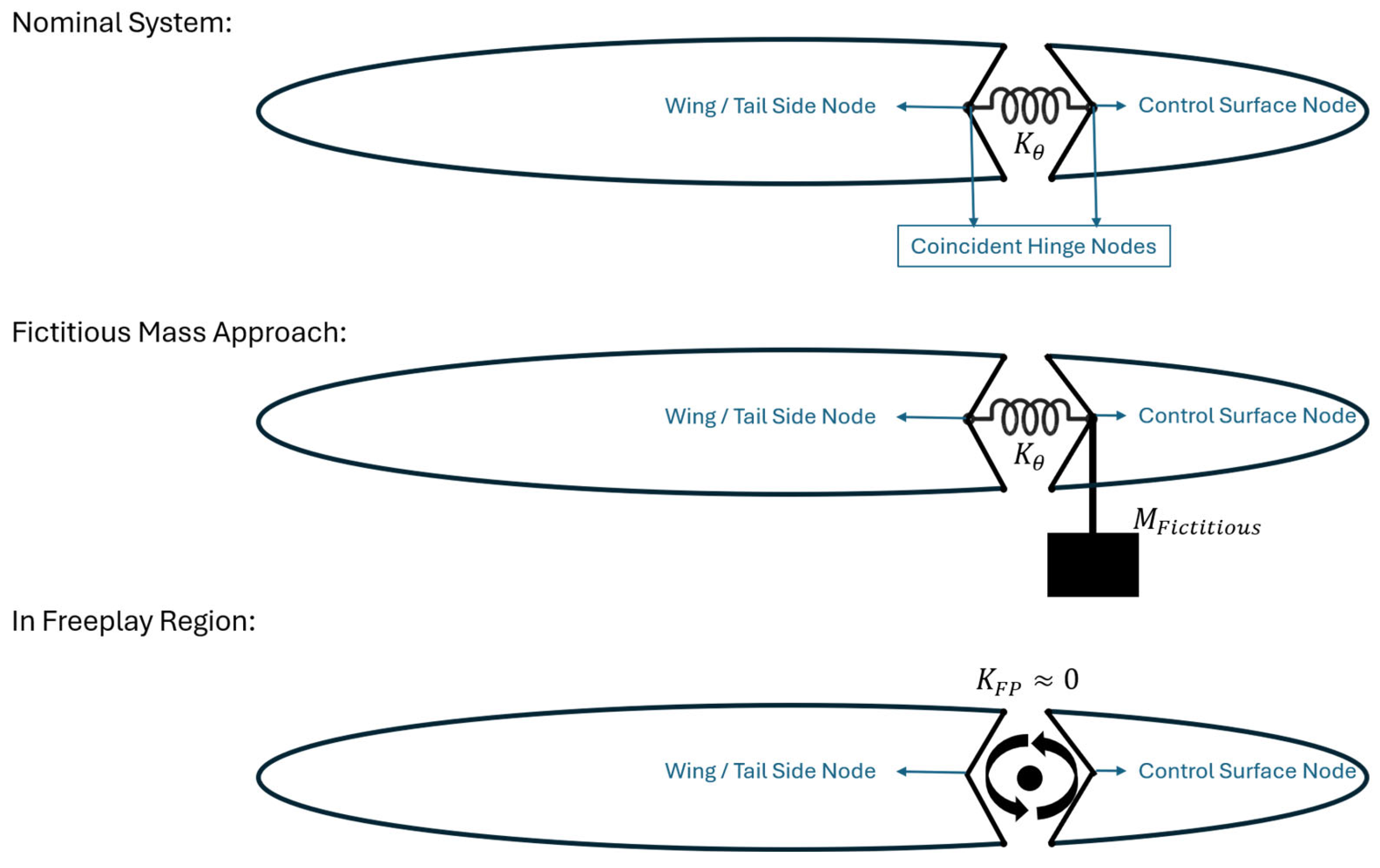
Table A1.
Comparison of natural frequencies of first three modes of the isolated wing–aileron model.
As demonstrated in Table A1, there is excellent agreement between the externally calculated natural frequencies and the NASTRAN results. The additional mode observed at ~1.98 Hz in the fictitious mass model accurately represents the characteristic local deformation mode introduced by the added local mass. Furthermore, when the control surface is allowed to act freely, the near-rigid body mode representing the free aileron rotation is successfully captured at ~0.275 Hz. In the simulations, the stiffness matrices corresponding to both the nominal and freeplay conditions are utilized, while only the nominal mass matrix is included in the calculations. By relying on this approach, the nonlinear freeplay condition is successfully and handled using a single modal matrix. This confirms that introducing a single fictitious mass term correctly bounds the dynamic problem over the large stiffness range without causing numerical instability.
References
- Bisplinghoff, R.L.; Ashley, H.; Halfman, R.L. Principles of Aeroelasticity; Dover Publications, Inc.: New York, NY, USA, 1975. [Google Scholar]
- Wan, Z.; Zhang, B.; Du, Z.; Yang, C. Aeroelastic Two-Level Optimization for Preliminary Design of Wing Structures Considering Robust Constraints. Chin. J. Aeronaut. 2014, 27, 259–265. [Google Scholar] [CrossRef] [Scilit]
- Tian, W.; Gu, Y.; Liu, H.; Wang, X.; Yang, Z.; Li, Y.; Li, P. Nonlinear Aeroservoelastic Analysis of a Supersonic Aircraft with Control Fin Free-Play by Component Mode Synthesis Technique. J. Sound. Vib. 2021, 493, 115835. [Google Scholar] [CrossRef] [Scilit]
- Karpel, M. Design for Active and Passive Flutter Suppression and Gust Alleviation; NASA CR-3482; NASA: Washington, DC, USA, 1981. [Google Scholar]
- Dunn, H.J. An Analytical Technique for Approximating Unsteady in the Time Domain; NASA Technical Paper 1738; NASA: Washington, DC, USA, 1980. [Google Scholar]
- Karpel, M.; Newman, M. Accelerated Convergence for Vibration Modes Using the Substructure Coupling Method and Fictitious Coupling Masses; University of Tel-Aviv: Tel Aviv, Israel, 1975. [Google Scholar]
- Karpel, M.; Wieseman, C.D. Modal Coordinates for Aeroelastic Analysis with Large Local Structural Variations. J. Aircr. 1994, 31, 396–403. [Google Scholar] [CrossRef] [Scilit] [PubMed]
- Karpel, M.; Raveh, D. Fictitious Mass Element in Structural Dynamics. AIAA J. 1996, 34, 607–613. [Google Scholar] [CrossRef] [Scilit] [PubMed]
- Karpel, M.; Wieseman, C.D. Time Simulation of Flutter with Large Stiffness Changes. J. Aircr. 1994, 31, 404–410. [Google Scholar] [CrossRef] [Scilit] [PubMed]
- Dimitriadis, G. Introduction to Nonlinear Aeroelasticity; Wiley: Hoboken, NJ, USA, 2017. [Google Scholar]
- Pereira, D.A.; Vasconcellos, R.M.G.; Hajj, M.R.; Marques, F.D. Effects of Combined Hardening and Free-Play Nonlinearities on the Response of a Typical Aeroelastic Section. Aerosp. Sci. Technol. 2016, 50, 44–54. [Google Scholar] [CrossRef] [Scilit]
- Panchal, J.; Benaroya, H. Review of Control Surface Freeplay. Prog. Aerosp. Sci. 2021, 127, 100729. [Google Scholar] [CrossRef] [Scilit]
- Gold, P.; Karpel, M.; Idan, M. Modeling and Control of Nonlinear Aeroservoelasticity Due to Actuator Free Play. In Proceedings of the 47th Israel Annual Conference on Aerospace Sciences, Haifa, Israel, 21–22 February 2007. [Google Scholar]
- Huang, R.; Hu, H.; Zhao, Y. Nonlinear Aeroservoelastic Analysis of a Controlled Multiple-Actuated-Wing Model with Free-Play. J. Fluids Struct. 2013, 42, 245–269. [Google Scholar] [CrossRef] [Scilit]
- Karpel, M.; Shousterman, A.; Maderuelo, C.; Climent, H. Dynamic Aeroservoelastic Response with Nonlinear Structural Elements. AIAA J. 2015, 52, 3233–3239. [Google Scholar] [CrossRef] [Scilit]
- Roizner, F.; Karpel, M. Parametric Flutter Margin Method for Aeroservoelastic Stability Analysis. AIAA J. 2018, 56, 1011–1022. [Google Scholar] [CrossRef] [Scilit]
- Yu, Q.; Damodaran, M.; Khoo, B.C. Nonlinear Aeroelastic Analysis of a Multi-Element Airfoil with Free Play Using Continuation Method. J. Fluids Struct. 2022, 109, 103482. [Google Scholar] [CrossRef] [Scilit]
- Bai, L.; Wu, Z.; Yang, C. Nonlinear Aeroelastic Characteristics of a Supersonic All-Movable Fin with Single or Multiple Freeplay Nonlinearities. Appl. Sci. 2023, 13, 1262. [Google Scholar] [CrossRef] [Scilit]
- Bai, L.; Wu, Z.; Yang, C. Nonlinear Aeroelastic Analysis of a Twin-Tail Boom UAV with Rudder Freeplay Nonlinearities. Chin. J. Aeronaut. 2024, 37, 276–296. [Google Scholar] [CrossRef] [Scilit]
- Ai, X.; Bai, Y.; Qian, W.; Li, Y.; Chen, X. Aeroelastic Investigation on an All-Movable Horizontal Tail with Free-Play Nonlinearity. J. Low Freq. Noise Vib. Act. Control 2024, 43, 634–650. [Google Scholar] [CrossRef] [Scilit]
- Xiang, Z.; Wang, L. Free-Play Nonlinearity Aeroelastic Studies on a T-Tail with a Segmented Rudder. Int. J. Struct. Stab. Dyn. 2025, 26, 2650234. [Google Scholar] [CrossRef] [Scilit]
- ZONA Tech. ZAERO Theoretical Manual V. 9.3; ZONA Technology, Inc.: Scottsdale, AZ, USA, 2017. [Google Scholar]
- MSC. MSC Nastran 2022.1-Reference Guide; MSC: Irvine, CA, USA, 2022. [Google Scholar]
- Stark, V.J.E. General Equations of Motion for an Elastic Wing and Method of Solution. AIAA J. 1984, 22, 1146–1153. [Google Scholar] [CrossRef] [Scilit] [PubMed]
- Rowell, D. 2. 14 Analysis and Design of Feedback Control Systems State-Space Representation of LTI Systems. 2002. Available online: http://web.mit.edu/2.14/www/Handouts/StateSpace.pdf (accessed on 13 December 2022).
- Napolitano, M.R. Aircraft Dynamics: From Modeling to Simulation; John Wiley & Sons, Inc.: Hoboken, NJ, USA, 2012. [Google Scholar]
- Cook, M.V. Flight Dynamics Principles: A Linear Systems Approach to Aircraft Stability and Control; Butterworth-Heinemann: Oxford, UK, 2013. [Google Scholar]
- Baldelli, D.H.; Chen, P.C.; Panza, J. Unified Aeroelastic and Flight Dynamic Formulation via Rational Function Approximations. J. Aircr. 2006, 43, 763–772. [Google Scholar] [CrossRef] [Scilit]
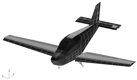
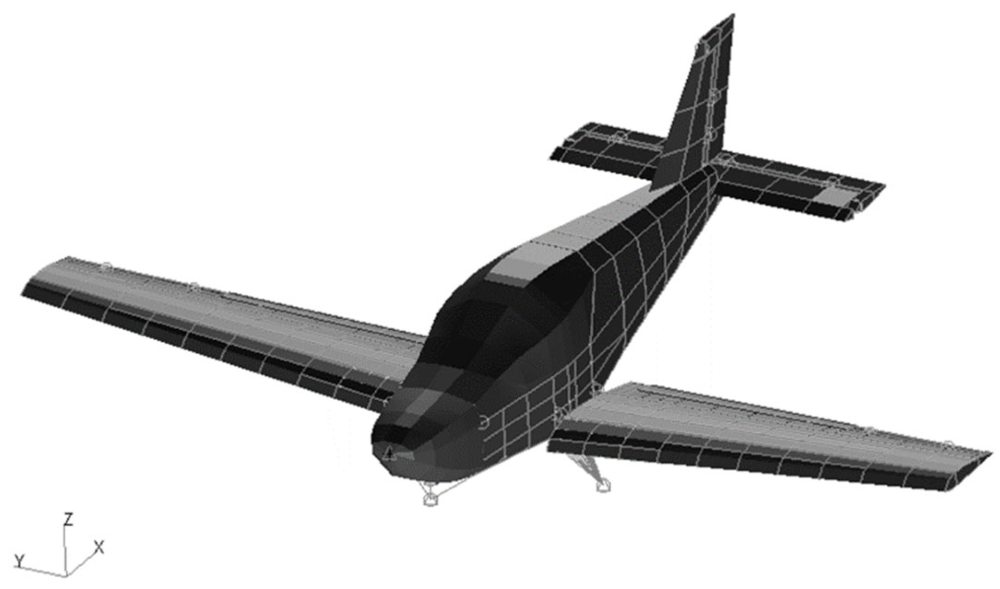
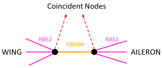
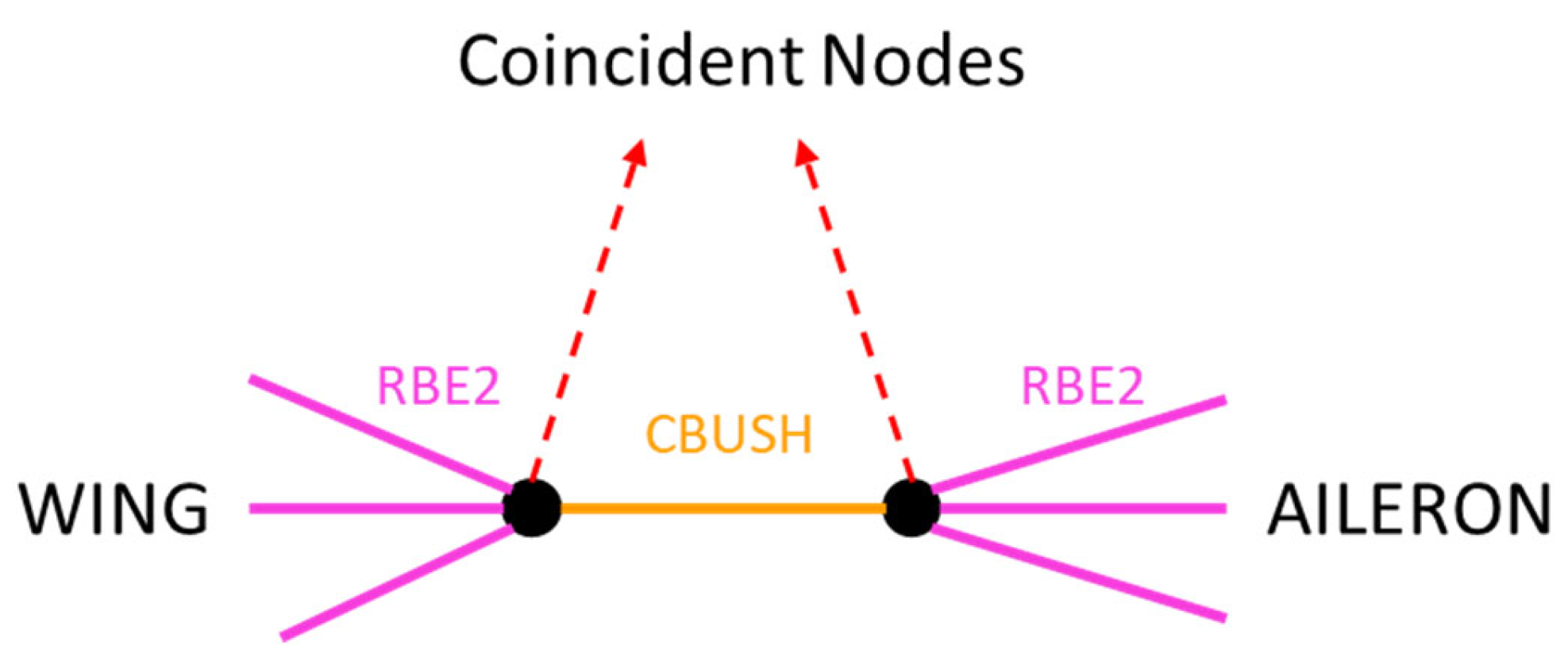
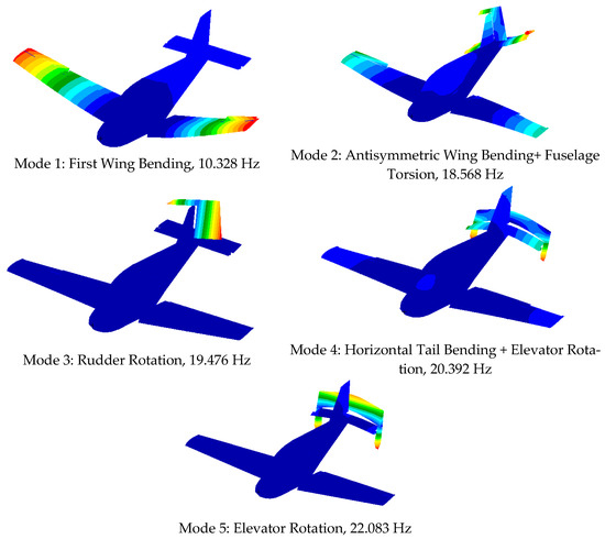
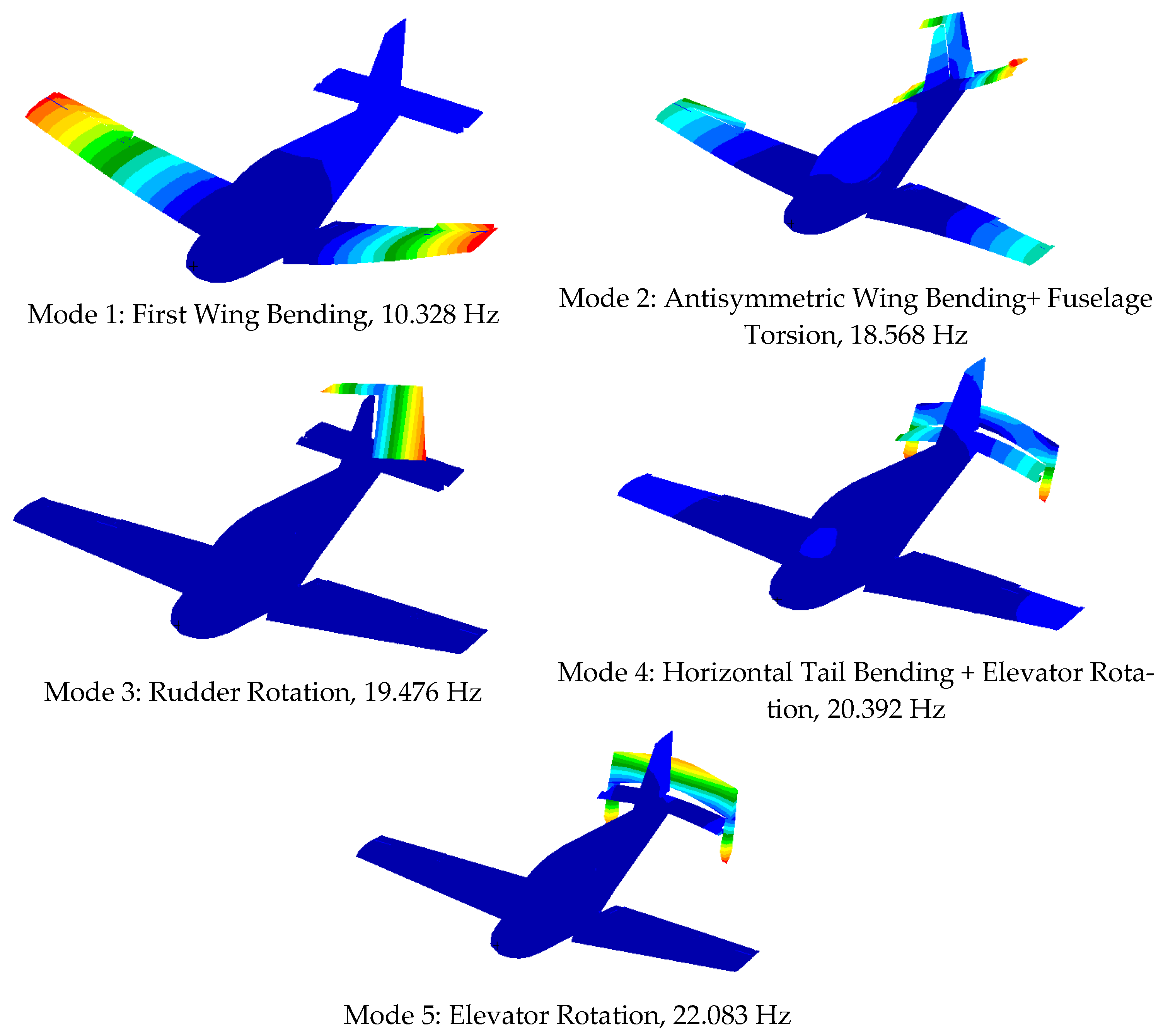
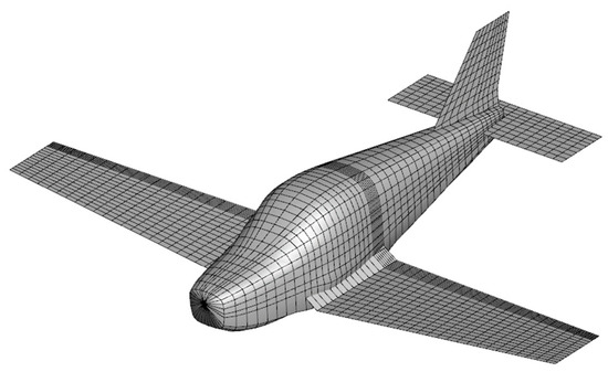
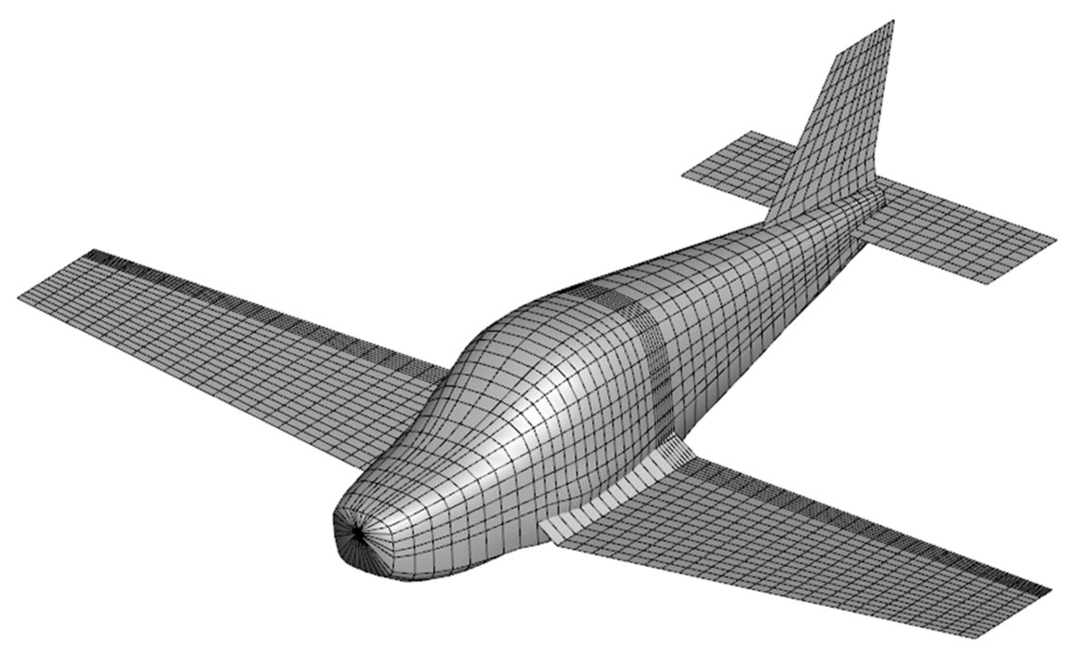
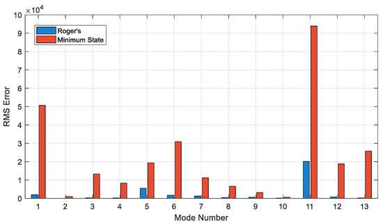
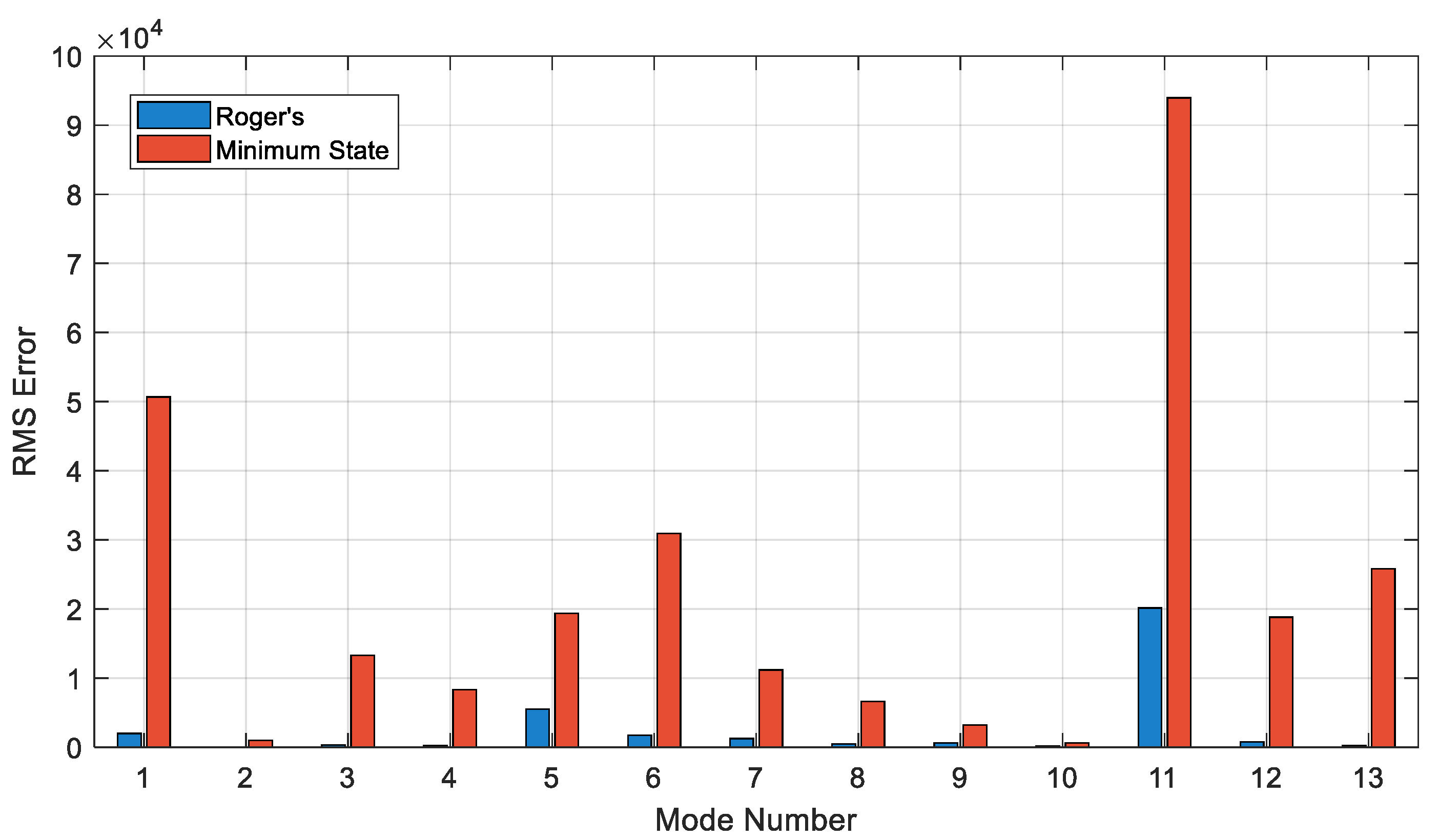
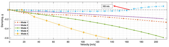
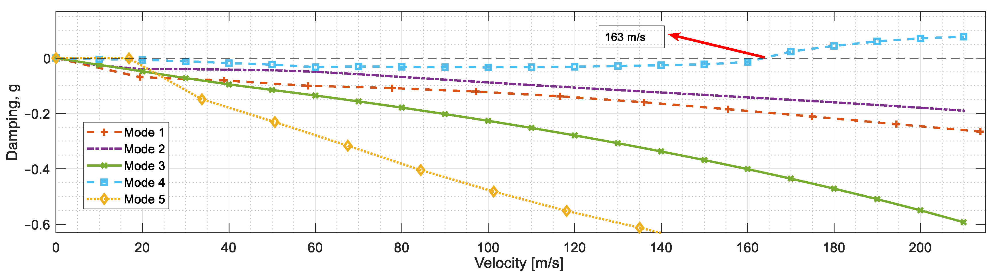
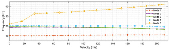
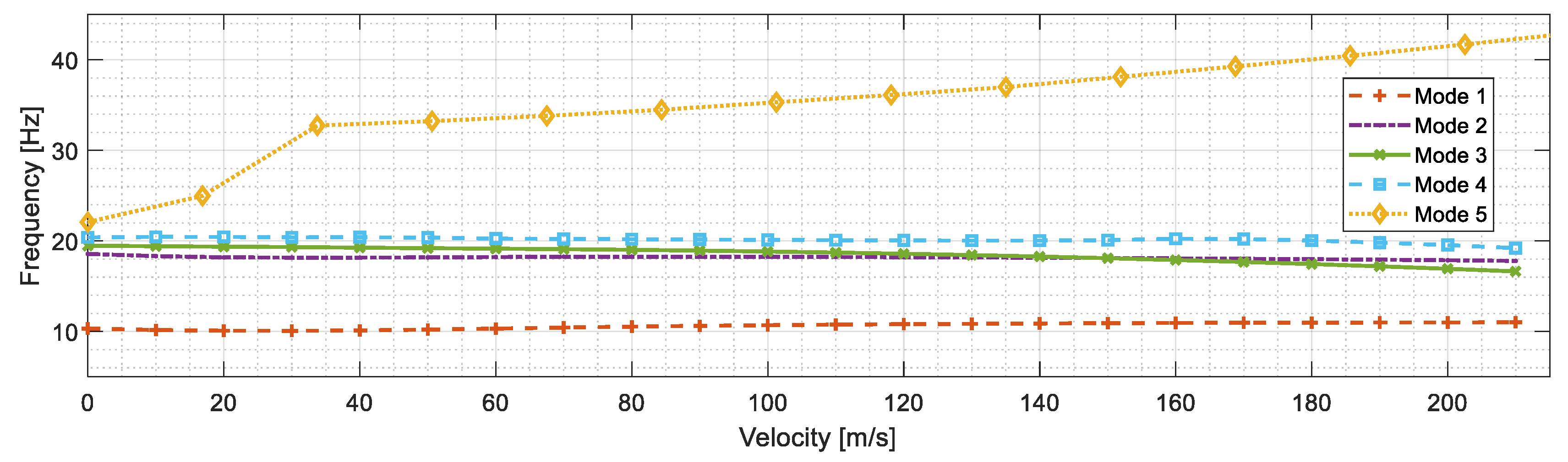
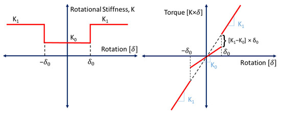
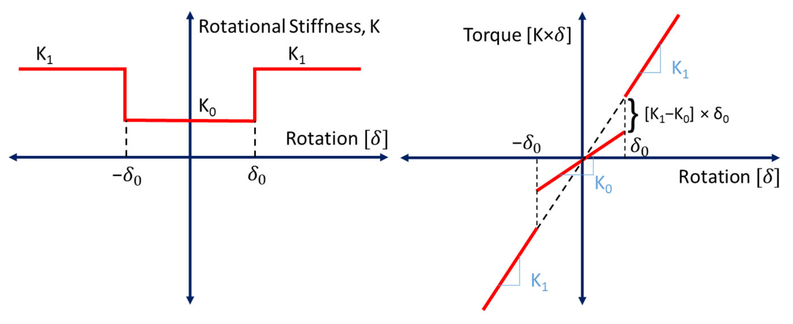
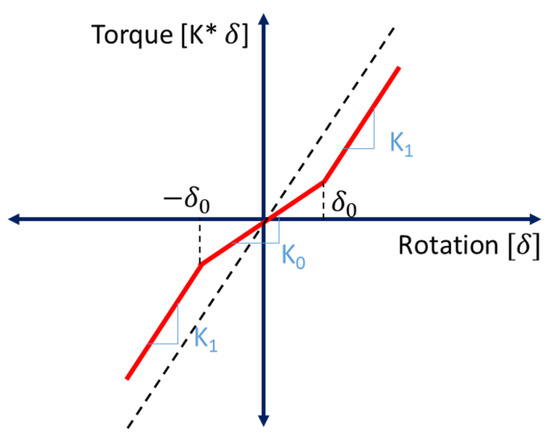
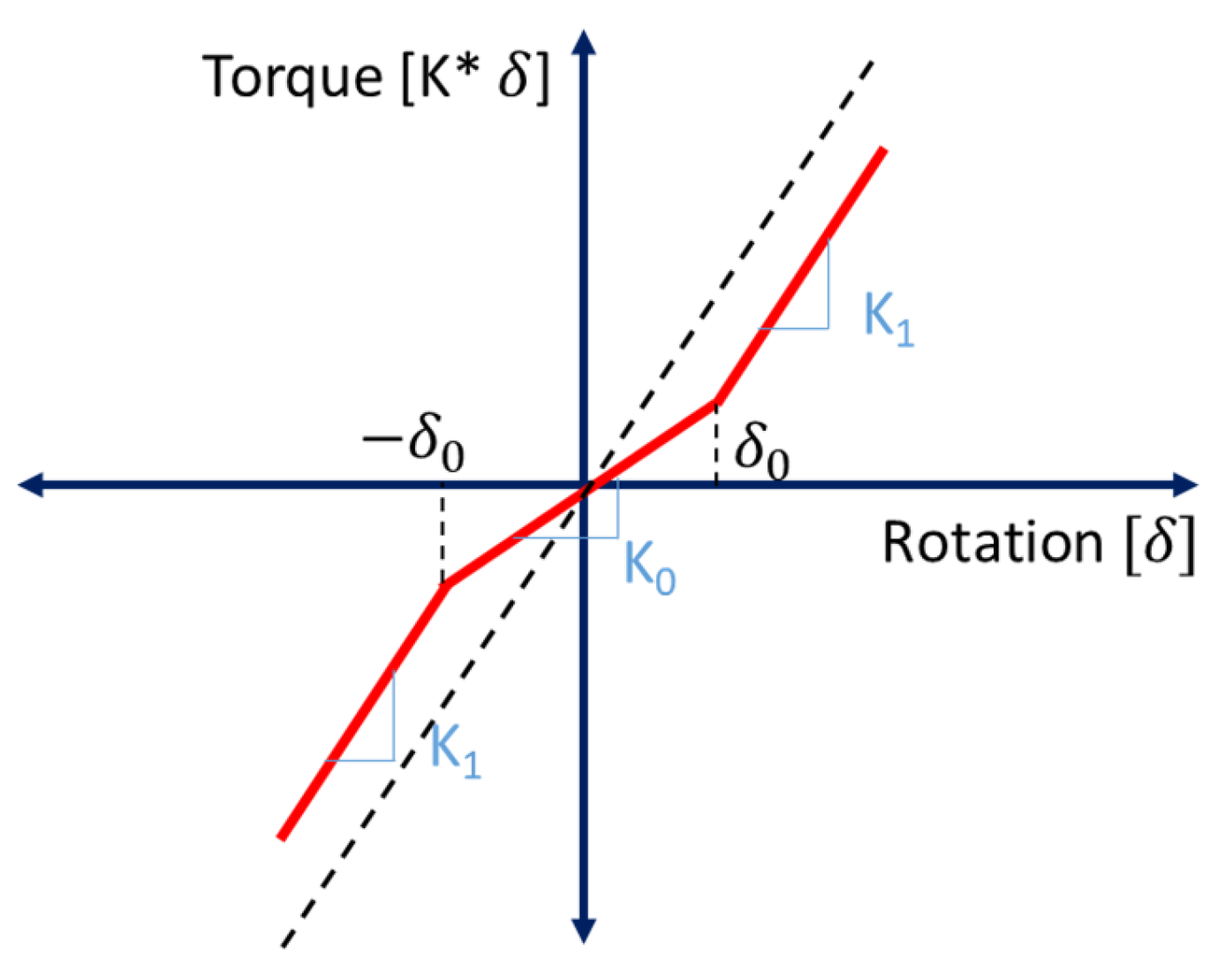
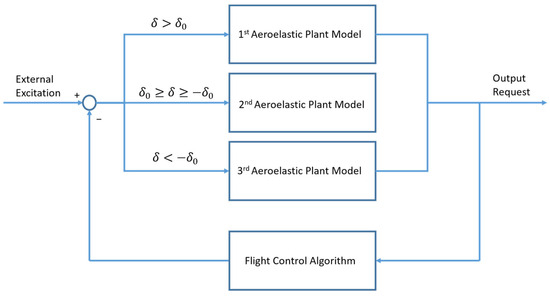
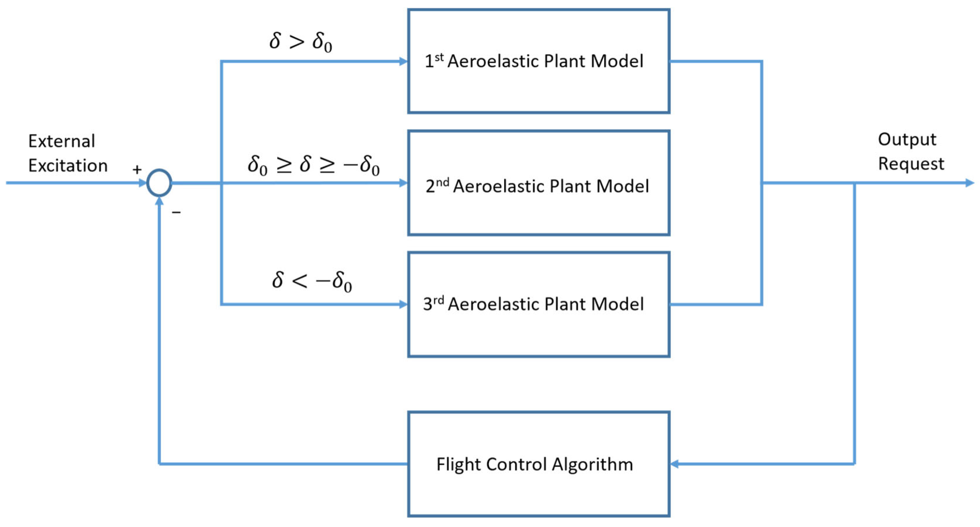
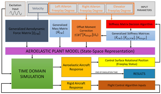
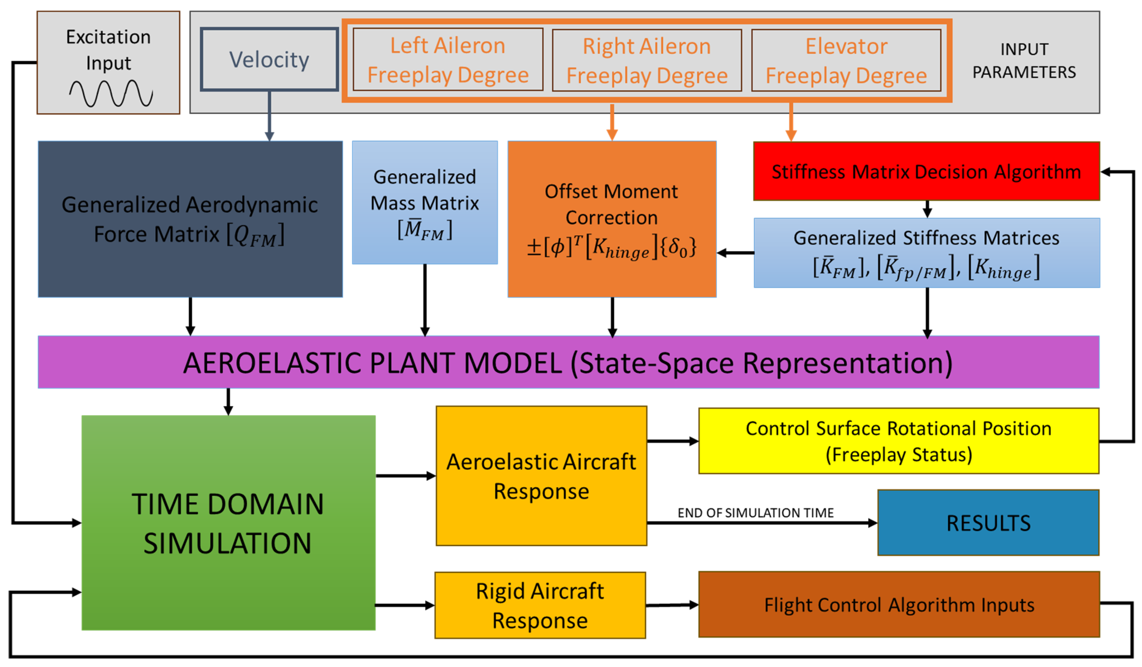
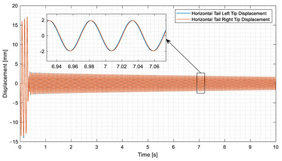
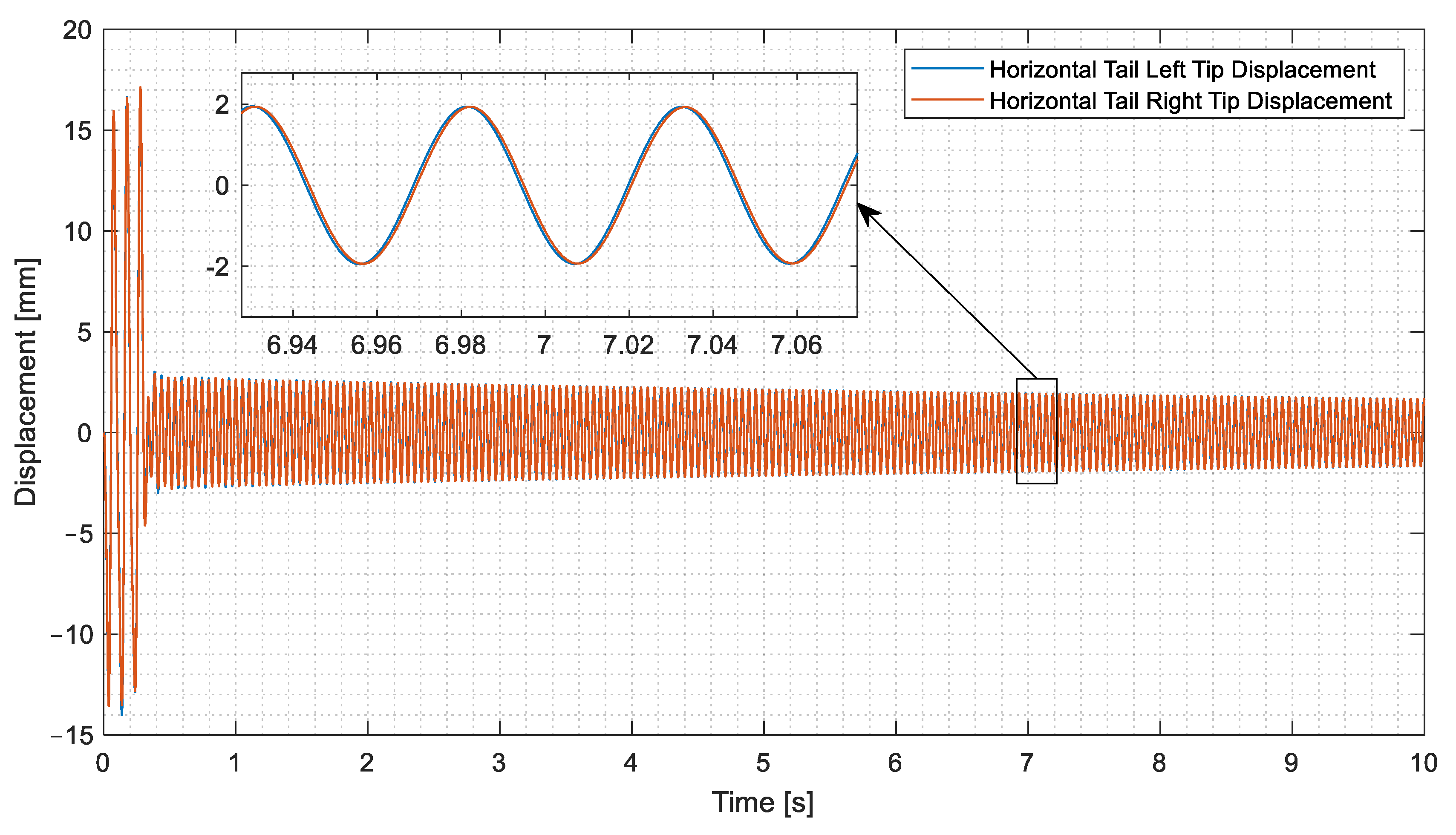
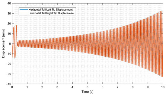
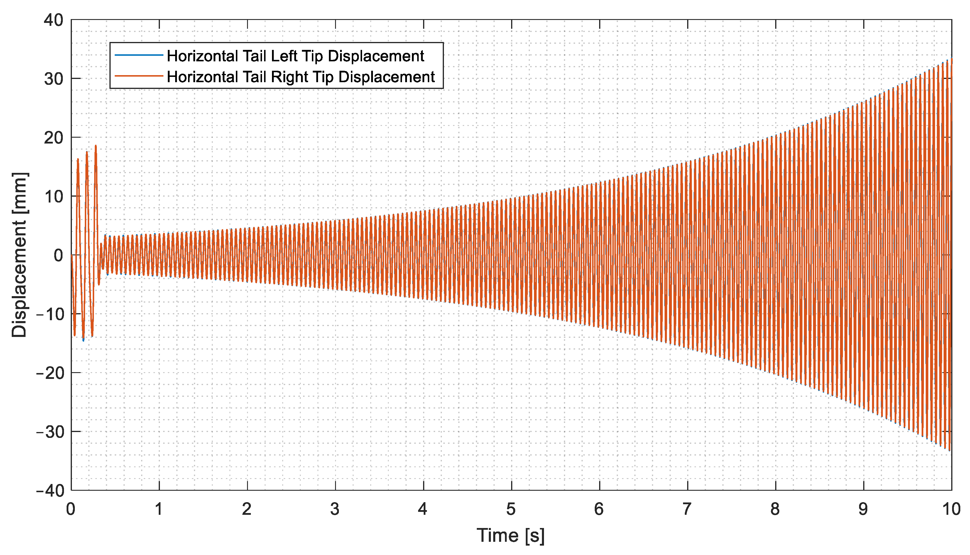
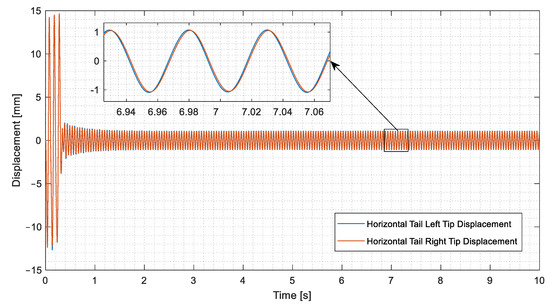
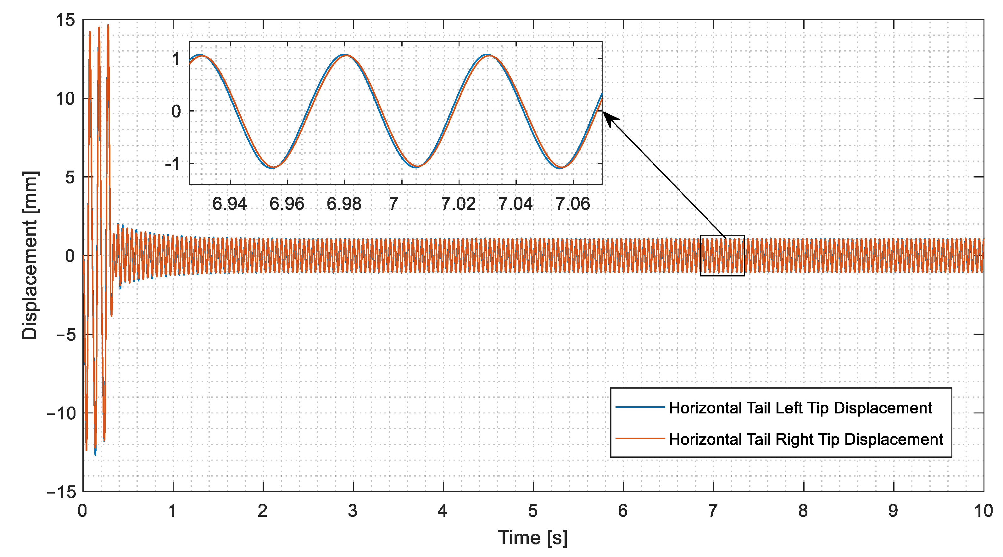
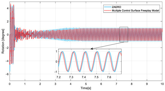
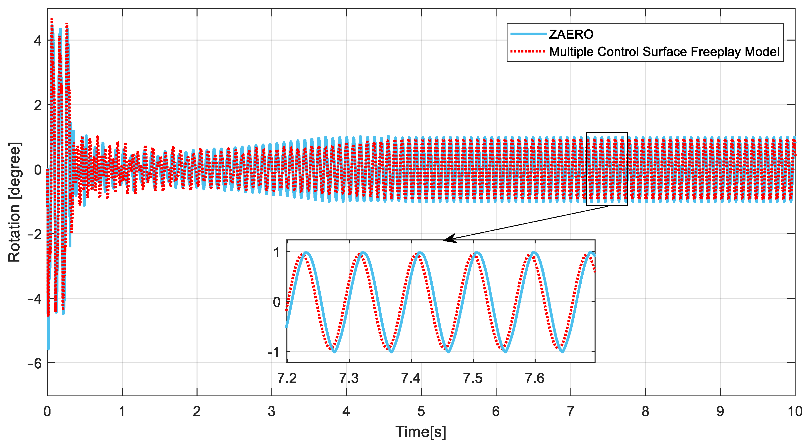
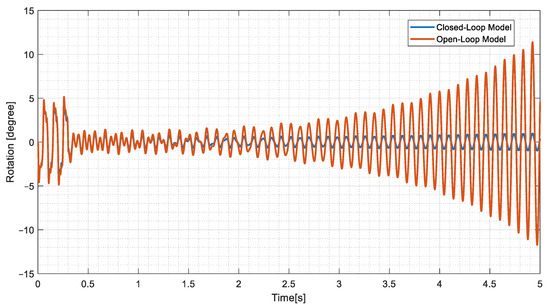
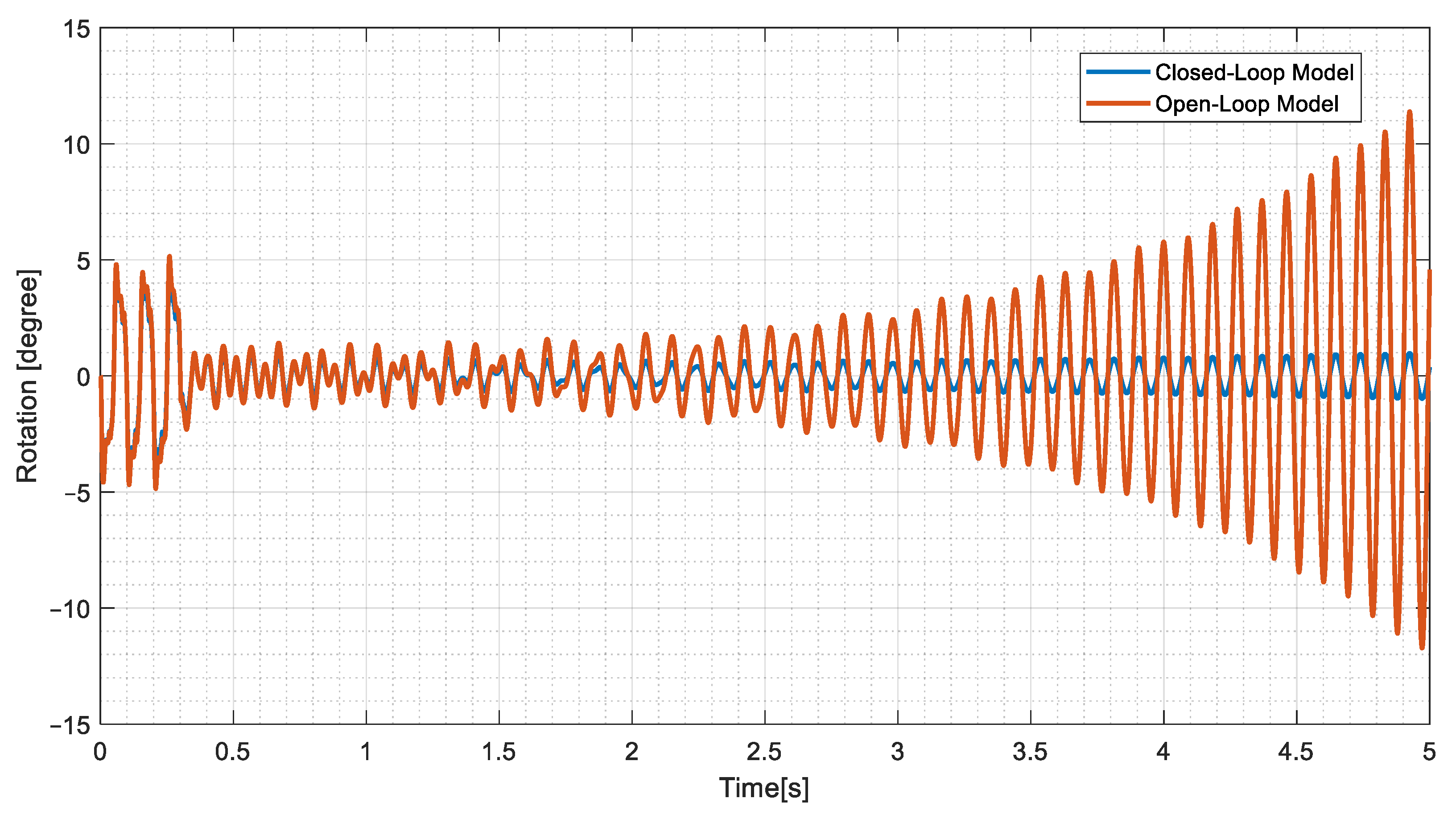
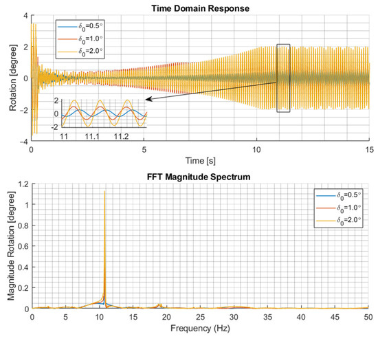
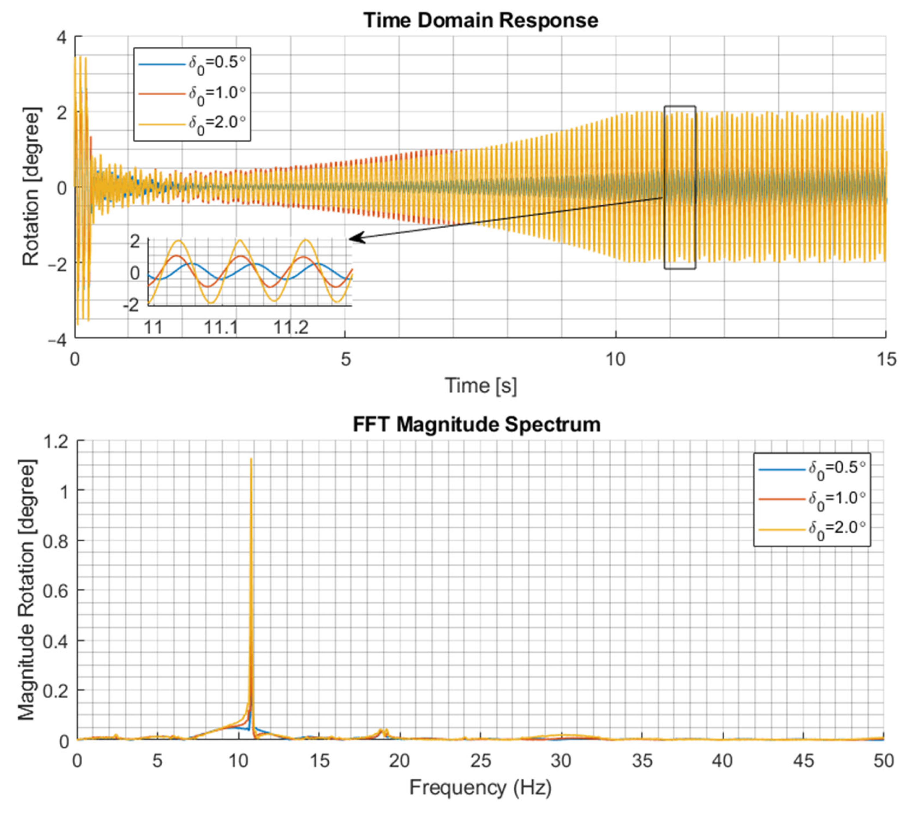
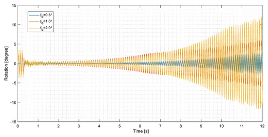
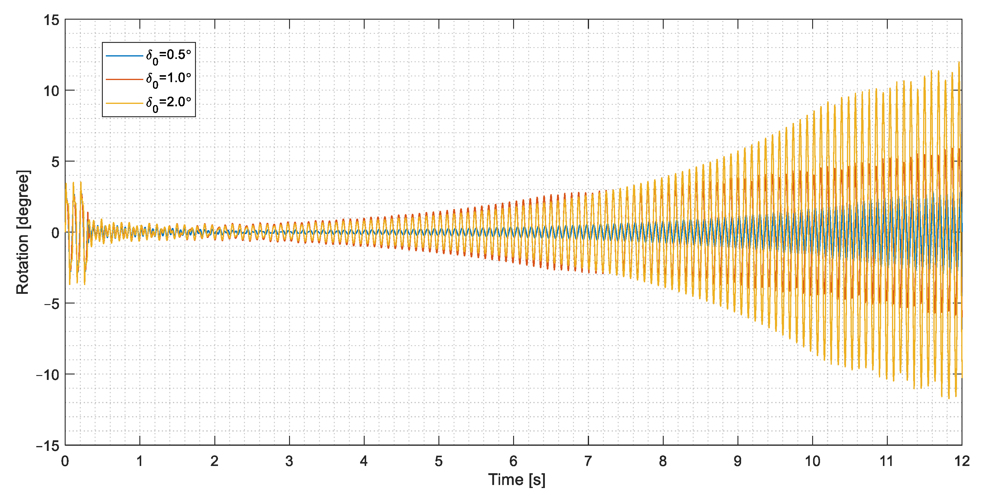
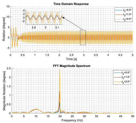
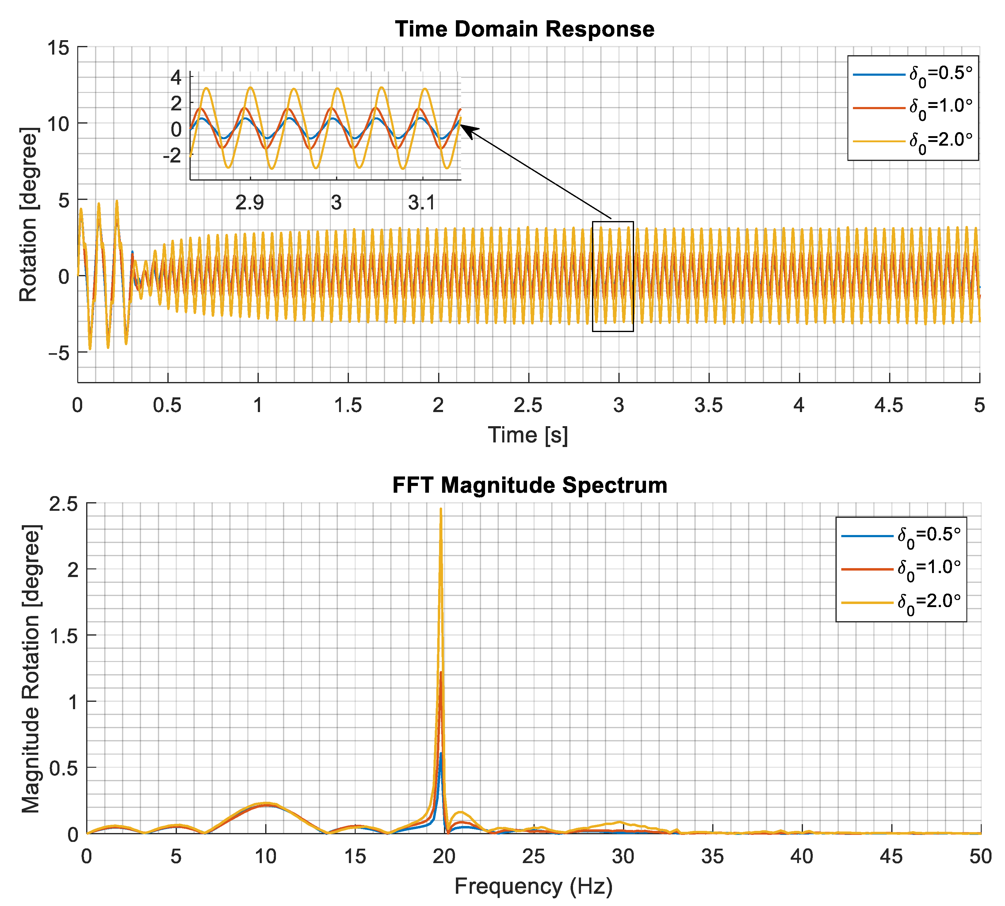
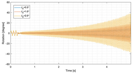
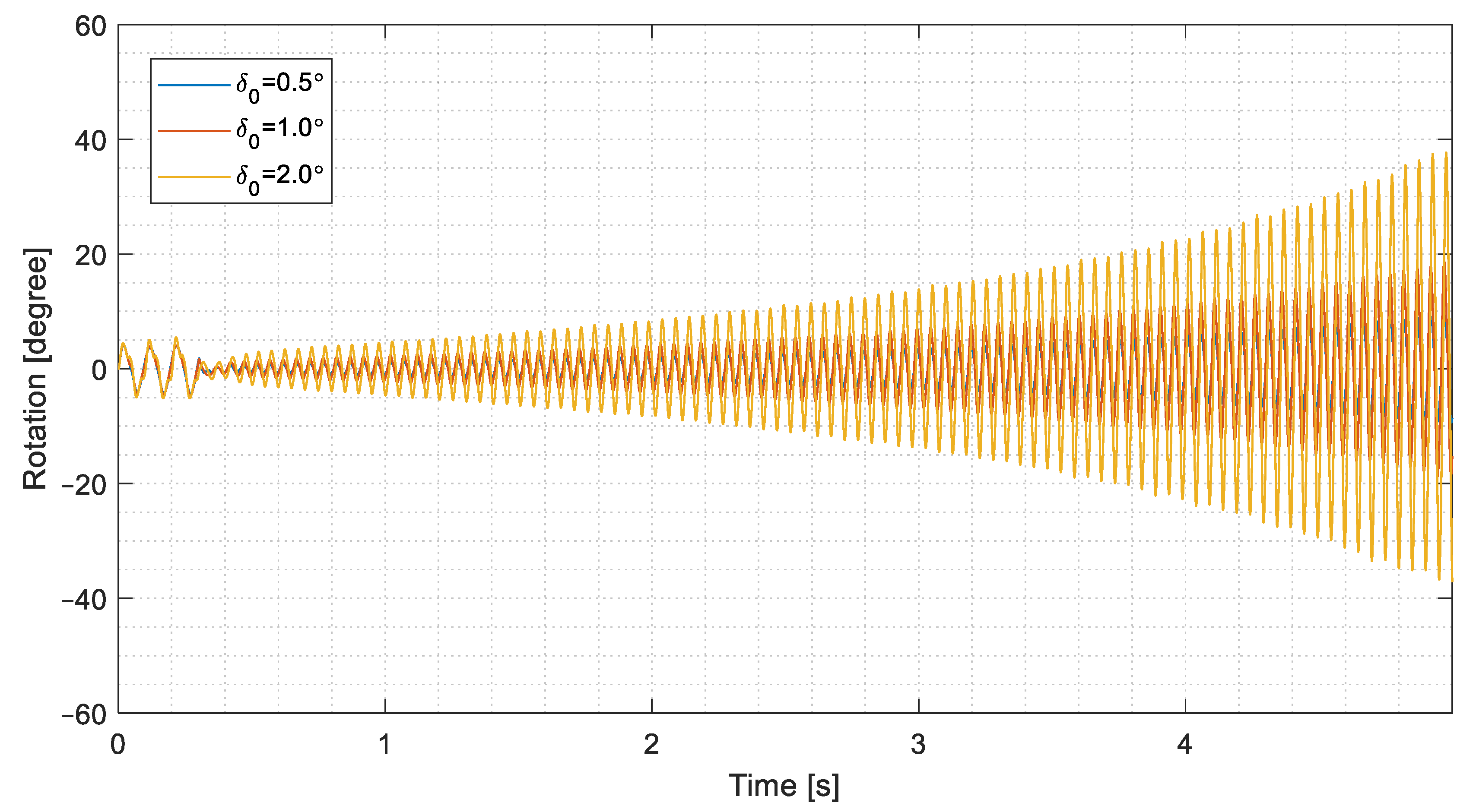
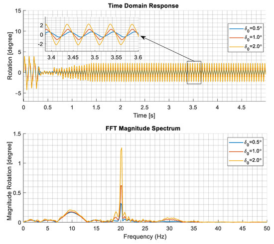
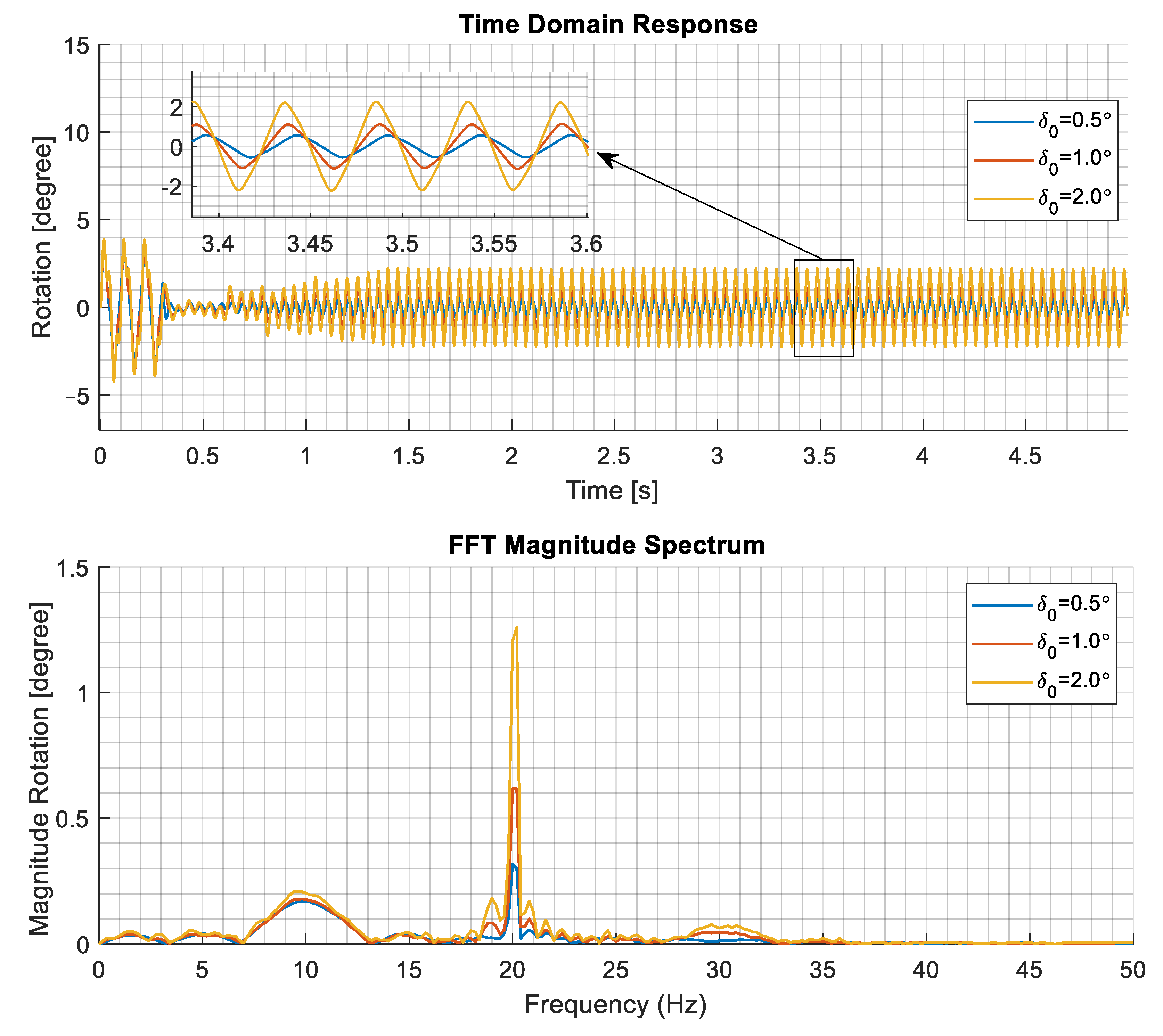
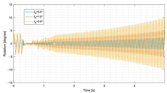
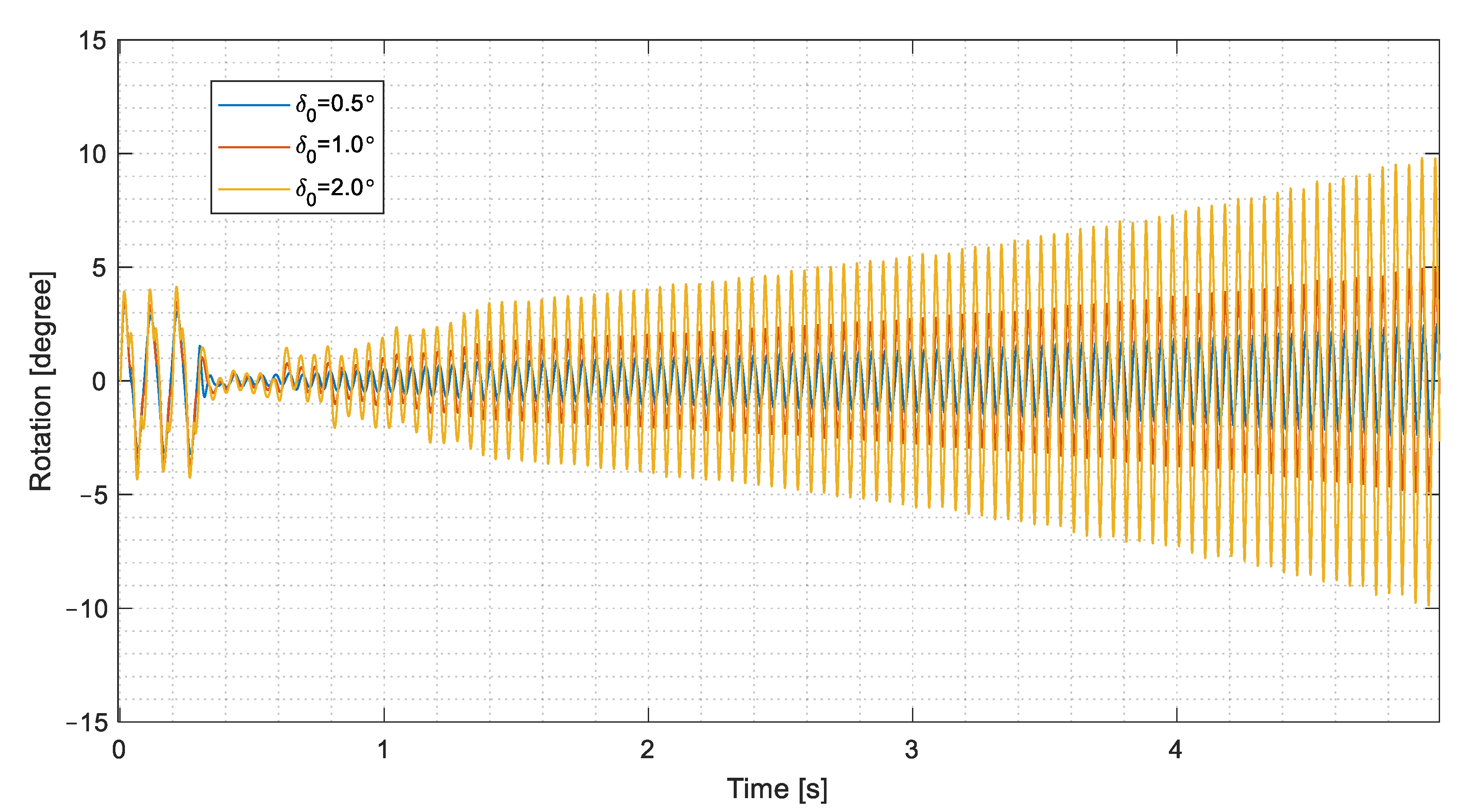
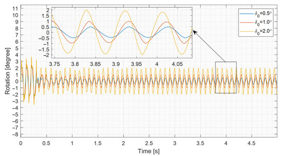
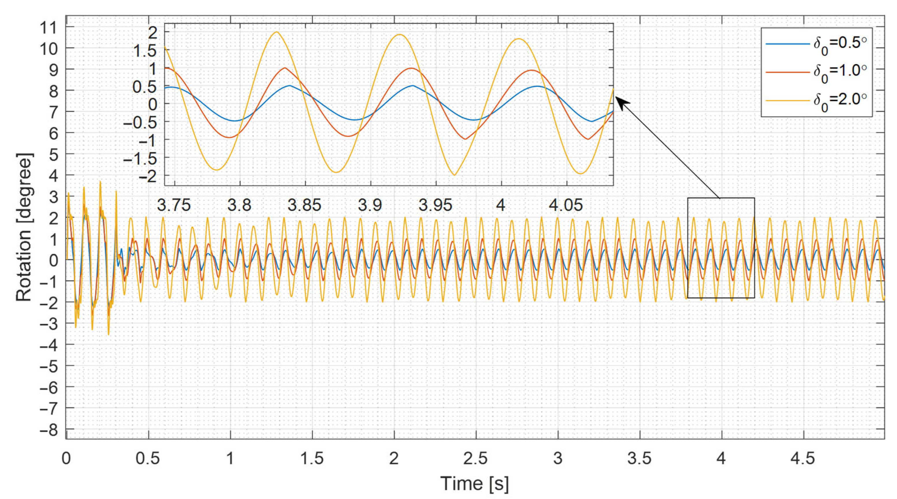
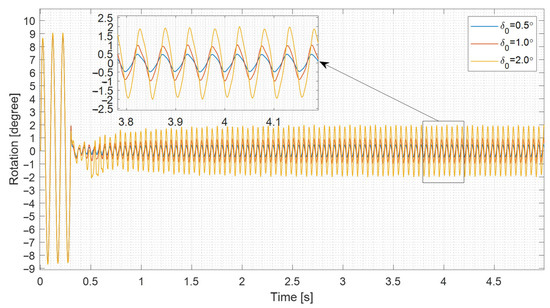
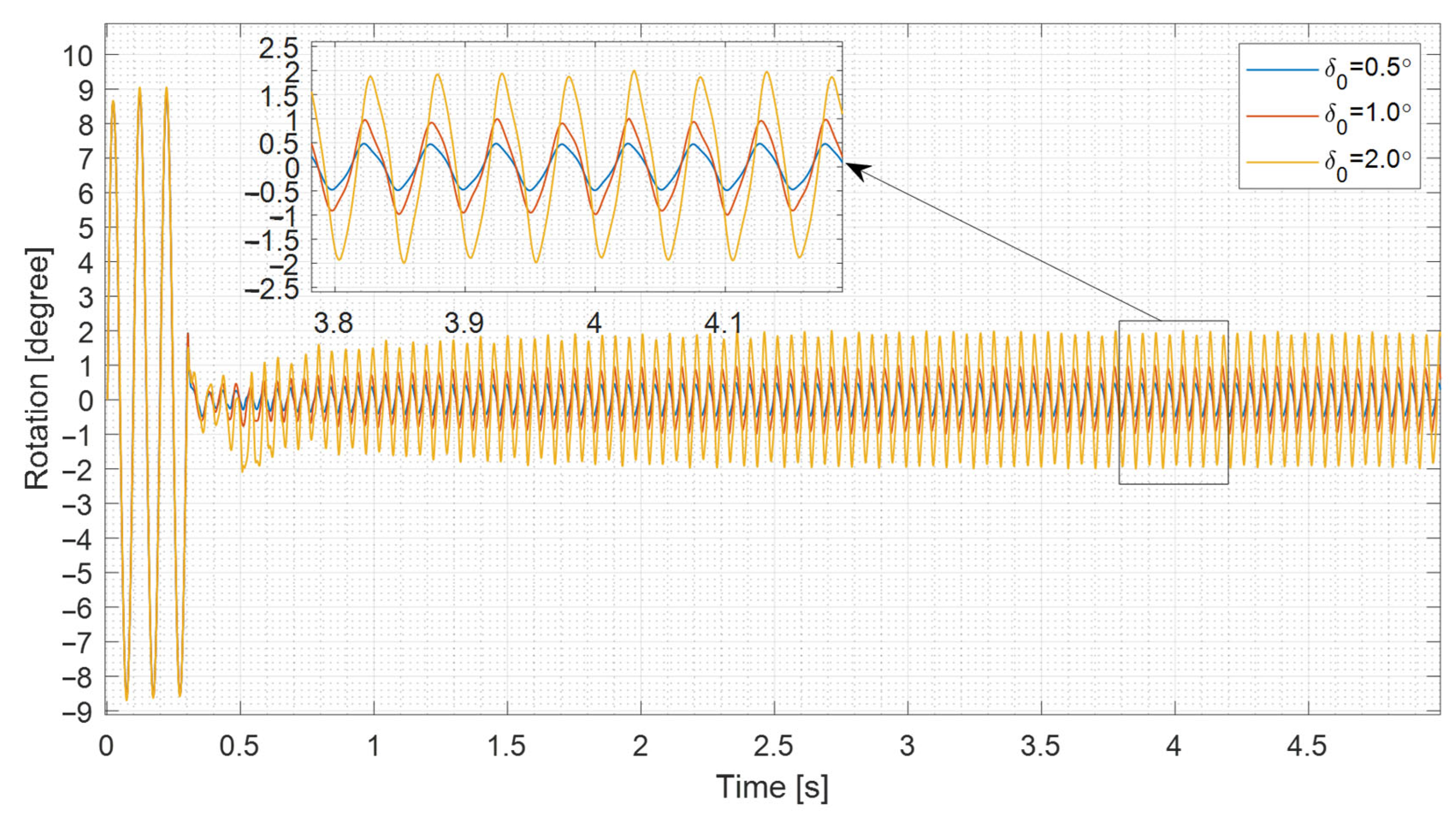

Disclaimer/Publisher’s Note: The statements, opinions and data contained in all publications are solely those of the individual author(s) and contributor(s) and not of MDPI and/or the editor(s). MDPI and/or the editor(s) disclaim responsibility for any injury to people or property resulting from any ideas, methods, instructions or products referred to in the content. |
© 2026 by the authors. Licensee MDPI, Basel, Switzerland. This article is an open access article distributed under the terms and conditions of the Creative Commons Attribution (CC BY) license.