


Abstract
Accurate thrust control is vital for efficient gas turbine engine operation, yet direct in-flight thrust measurement is unavailable. Most engines rely on speed control schedules, which suffer from unplanned dead zones and poor throttle-to-thrust linearity—compromising pilot handling and fuel economy. We propose a robust thrust control schedule to improve the thrust-to-throttle relationship. It integrates two intermediate/idle thrust estimators, a degradation estimator, and a reference thrust estimator. The first intermediate/idle thrust estimator provides baseline estimates of intermediate and idle thrust. The degradation estimator compensates thrust deviations caused by engine degradation. The second intermediate/idle thrust estimator updates its estimates online using compensated estimates to track degradation. The reference thrust estimator then uses outputs from the second estimator and linearly interpolates the current power lever angle to determine reference thrust. The proposed schedule is evaluated under the considered degradation conditions. CLM-based simulations evaluate its effectiveness during the early-stage degradation period, while the micro-turbojet ground experiment demonstrates the proof-of-concept implementation of the outer thrust-loop structure.
1. Introduction
Thrust, as a key performance parameter of gas turbine engines, is essential for the successful execution of various flight missions [1]. Different operational scenarios—such as takeoffs [2], landings [3], supersonic transitions, and flight attitude control—impose specific and often stringent demands on thrust control [4]. For example:
Takeoffs and landings: Considering constraints such as runway length, takeoff time, and braking performance, engines must provide higher thrust during take-offs and lower thrust during landings. For carrier-based aircraft [5], these demands become even more stringent, as the responsiveness to thrust variation significantly affects the pilot’s handling experience and the success rates of takeoffs and landings.
Supersonic flight and maneuvers: Achieving supersonic speeds often requires activating the afterburning state to deliver greater thrust, which is also essential for performing certain high-performance maneuvers.
Thrust balance in multi-engine aircraft: For aircraft equipped with multiple engines, maintaining balanced thrust output across the engines is crucial for ensuring stability and preventing deviations from the intended flight trajectory.
Flight attitude control: In addition to managing control surfaces, further thrust management can enhance the precision and responsiveness of flight attitude adjustments [6], contributing to improved overall flight performance.
To meet these demands, pilots must familiarize themselves with the throttle-to-thrust characteristics, manipulate the throttle precisely, and continuously assess whether the thrust variation is in line with expectations. If the expected control effect is not achieved, the throttle needs to be further adjusted. However, repeated throttle adjustments can undoubtedly increase the pilot’s workload [7] and even affect the execution of flight missions. During this period, suboptimal fuel consumption may also arise. Therefore, it is preferable to integrate these demands into the design of control schedules rather than relying only on the pilot. Unfortunately, since in-flight thrust cannot be measured [8,9], almost all engines do not have the conditions to deploy a thrust control schedule, and can only use a speed control schedule as an alternative [10,11]. Owing to the correlation between rotor speed and thrust, it enables indirect thrust control, meeting the thrust demands of most flight missions. However, what the pilot directly perceives is the change in engine thrust, not the change in rotor speed. As a result, it inevitably brings some issues, which are summarized as follows:
- Unplanned dead zones of thrust variation are observed near the engine’s idle and intermediate states, leading to an undesirable piloting experience.
- The linearity of the throttle-to-thrust relationship is notably suboptimal, and this uneven thrust variation is also unfavorable for throttle manipulation.
Advances in thrust estimation technologies now enable the integration of a virtual thrust sensor within the engine control system [12,13,14,15], laying the foundation for the advancement of thrust control. Jonathan S. Litt, et al. from NASA first introduced the concept of engine performance degradation mitigating control, also referred to as thrust control [16,17,18,19]. It can maintain the throttle-to-thrust relationship during engine performance degradation, and alleviate pilot workload by eliminating the need for manual throttle adjustments [20]. Inspired by their research, scholars primarily focus on mitigating engine degradation, aiming to offset thrust loss through thrust control. For example, Yan et al. [21] proposed a neural network control method for thrust degradation mitigation based on variable incremental linear programming optimization, which reduces engine thrust degradation by adjusting the engine command signal. Zhao et al. [22] designed a control system for engine performance degradation recovery, utilizing an inner loop to control engine speed and an outer loop to control thrust. Li et al. [23] conducted research on performance degradation mitigation control, achieving direct thrust control to improve engine autonomous control.
Although such thrust compensation is effective for the engine’s throttling state, it distorts the throttle-to-thrust relationship, thereby degrading its linearity. Furthermore, near the intermediate state, compensatory actions for thrust loss may prematurely activate limit control schedules, potentially enlarging the unplanned dead zones in thrust variation. However, it is important to note that, due to the presence of limit control schedules, thrust loss at the intermediate state is irrecoverable. In practical engineering, common strategies for counteracting engine degradation include: (1) engine overhauls; (2) engine cleanings; (3) adjustment of nozzle control schedules; and (4) moderate increases in the limited value of the total temperature at the low-pressure turbine exit.
Furthermore, most studies utilize the onboard engine state-space model for thrust control. This model is developed by linearizing the engine component-level model (CLM) [24,25]. However, ensuring its accuracy across the entire flight envelope and under various engine states remains a challenge [26,27], inevitably affecting thrust control accuracy. Additionally, due to the limited computing speed and memory capacity of existing onboard equipment, almost no in-service engines are equipped with onboard models, particularly the CLM. As a result, model-based thrust control may not be the most suitable solution for current engineering applications.
To improve the throttle-to-thrust relationship, this study proposes a robust thrust control schedule (RTCS) consisting of two intermediate/idle thrust estimators, a degradation estimator, and a reference thrust estimator. Compared to the traditional speed control schedule, the proposed RTCS effectively narrows the range of unplanned dead zones in thrust variation and improves the linearity of the throttle-to-thrust relationship under the considered engine-performance degradation conditions. Thanks to this, the fuel consumption under different engine states becomes more rational. Furthermore, it eliminates the need for onboard engine models and can be encapsulated as an independent module for integration into the controller. Ultimately, the proposed RTCS, combined with our previously developed thrust estimation method and a supporting PI controller, establishes a closed-loop thrust control system. The main contributions of this study are outlined as follows:
- From the perspective of the pilot’s handling experience, this study offers a detailed analysis of the issues associated with the traditional speed control schedule and its underlying causes, which have not been explicitly addressed in previous research.
- An RTCS is designed to narrow the range of unplanned dead zones in thrust variation and improve the linearity of the throttle-to-thrust relationship, while a degradation estimator is introduced to improve its adaptability under the considered engine-performance degradation conditions.
- A sequentially stacked neural network (SSNN) is employed to model the component that needs to be updated online in the RTCS, reducing resource consumption.
- A triple-closed-loop control system for thrust, speed, and fuel is established without utilizing the onboard engine model.
2. Problem Statement
2.1. Main Fuel Control System and Speed Control Schedule
For the gas turbine engine depicted in Figure 1, the main fuel control system consists of two loops: a fuel control loop and a speed control loop, as shown in Figure 2. The terms HPC, HPT, and LPT denote the high-pressure compressor, high-pressure turbine, and low-pressure turbine, respectively. The engine’s control/input and output parameters are outlined in Table 1.
Figure 1.
Schematic diagram of a gas turbine engine. The numeric labels denote engine station numbers, and their correspondence with the parameters in Table 1 is explained in the text.
Figure 2.
Schematic diagram of the main fuel control system.
Table 1.
Description of the engine’s control/input and output parameters.
The numeric labels in Figure 1 denote engine station numbers rather than compo-nent indices. These station numbers are used as subscripts in the corresponding param-eters listed in Table 1. Specifically, station 1 denotes the intake entry; station 2 denotes the fan entry and corresponds to pt2 and Tt2; station 15 denotes the external duct entry and corresponds to pt15 and Tt15; station 16 denotes the external duct exit; station 25 denotes the HPC entry and corresponds to pt25 and Tt25; station 31 denotes the HPC exit and corresponds to pt31 and Tt31; station 4 denotes the HPT entry; station 45 denotes the LPT entry; station 6 denotes the LPT exit and corresponds to pt6 and Tt6; station 7 denotes the afterburner entry; station 8 denotes the nozzle throat and corresponds to A8; and station 9 denotes the nozzle exit and corresponds to A9.
Fuel control loop: In the fuel control loop, the fuel controller aims to minimize the tracking error of the fuel flow by adjusting the metering valve’s opening area, thereby ensuring that the fuel delivery meets the desired target value. The tracking error in fuel flow is defined as follows:
where Wf,ref and Wf,cal denote the reference and calculated values of the fuel flow, respectively. Wf,ref is determined in the speed control loop.
Since the fuel flow is not measured directly, it is calculated as follows:
where cf denotes the flow coefficient. Av denotes the metering valve’s opening area. ρf denotes the fuel density. Δpv denotes the pressure difference across the metering valve. Δpv is usually designed to remain constant, allowing fuel flow to be adjusted solely by changing Av.
Speed control loop: The speed control loop comprises a speed controller, a limit controller and a series of fuel control schedules. The speed and limit controllers work together to determine the steady-state fuel flow Wf,ste. Before the limit parameters reach their limited values, Wf,ste is determined solely by the speed controller. Taking the nH-based control for example, its tracking error is expressed as follows:
where nH,ref and nH,mea denote the reference and measured values of nH, respectively.
To ensure engine safety, the limit controller is designed to prevent any limit parameters from surpassing their limited values. For the nH-based control, the limit parameters include nL, nL,cor, nH,cor, Tt6, and pt31. Among them, nL,cor and nH,cor represent the corrected values of nL and nH, respectively.
The reasons for limiting these parameters are outlined as follows:
- nL is limited due to the strength constraints of the low-speed rotor.
- nL,cor and nH,cor are limited due to the aerodynamic stability constraints of the fan and HPC. Additionally, nL,cor is also limited by matching constraints of the inlet corrected airflow.
- Tt6 is limited due to the temperature resistance and lifespan constraints of turbine components.
- pt31 is limited due to the compressive strength constraints of the engine casing.
Assuming χ represents one of the limit parameters, the tracking error between the limited and measured values is expressed as follows:
where χlim and χmea denote the limited and measured values of this limit parameter, respectively.
Additionally, a series of other fuel control schedules also determine the value of Wf,ref. In the Min-Max control configuration [28], Wf,ref is ultimately expressed as follows:
where Wf,dcc, Wf,acc, Wf,min and Wf,pro denote the fuel flow calculated by the deceleration control schedule, acceleration control schedule, limit control schedule of the minimum fuel flow, and protection control schedule, respectively. The Min–Max control logic may vary slightly across different engines. Moreover, in the event of engine over-speed or over-temperature conditions, the protection control schedule may semi-cut off or fully cut off the fuel supply by manipulating actuators, such as the fuel return valve, bypassing both the fuel controller and the metering valve. The term “Min–Max” here follows the conventional terminology of aero-engine fuel-control logic and denotes a selection/arbitration mechanism among precomputed fuel commands. It is not a mathematical Min–Max optimization problem.
In the speed control loop, the speed control schedule is designed to determine nH,ref. For most engines in service, it generally takes the following form:
where PLA denotes the power lever angle. The subscripts “idl” and “int” denote the idle and intermediate states, respectively.
Pilot-based thrust control loop: In this dual-closed-loop control system, an implicit pilot-based thrust control loop is also present. According to Equation (6), PLA is not directly linked to thrust. Thrust is, in fact, controlled by the pilot, who simultaneously performs multiple roles, including those of thrust sensor, controller, and actuator. Specifically, the pilot must continuously assess whether the thrust variation aligns with mission requirements and adjust the throttle accordingly.
2.2. Issues, Proposed Solutions and Requirements
2.2.1. Issues
As shown in Figure 3, the main issues with the speed control schedule are concentrated in two aspects: (1) Unplanned dead zones in thrust variation; (2) Poor linearity in the throttle-to-thrust relationship. The inherent indirectness in thrust control makes these issues largely unavoidable. The desired throttle-to-thrust relationship, including the prescribed planned flat zones, is described in Appendix A.1. Figure 3 is a schematic illustration of the main issues caused by the speed control schedule. The formal desired throttle-to-thrust relationship with prescribed planned flat zones is defined in Appendix A.1.
Figure 3.
Issues with the speed control schedule. (a) Unplanned dead zone near a limit-control activation region. (b) Poor linearity in the throttle-to-thrust relationship. The arrows and blue dots indicate the direction and representative points of throttle/thrust variation.
The first issue arises when a limit control schedule is activated prematurely [29]. For instance, a reduction in HPC efficiency leads the main fuel control system, which takes nH as the control target, to inject additional fuel to maintain the reference speed. This, in turn, results in an increase in Tt6 [30]. As the pilot progressively increases throttle input, the temperature may prematurely reach its allowable limit, triggering the corresponding temperature limit control schedule sooner than expected. Additionally, at the left boundary of the flight envelope, reducing throttle to bring the engine to its idle state can sometimes cause the limit control schedule of the minimum fuel flow to activate prematurely. This control schedule ensures that, under rarefied air conditions, a reasonable fuel-to-air ratio is maintained to support stable combustion.
The second issue is related to the nonlinear nature of the speed-to-thrust relationship [31], which is further exacerbated by various uncertainties, such as engine performance degradation.
2.2.2. Proposed Solutions
To address the issues above, this study proposes a solution in the form of a thrust control schedule, with the expected throttle-to-thrust curve as the target. In this study, the term “schedule” refers to a reference-generation law in the aero-engine control system. Specifically, the proposed RTCS determines the reference thrust according to flight condition, engine state, and power lever angle. It should be distinguished from the thrust-tracking controller itself. Based on our previously developed thrust estimation method, a thrust control loop can be constructed, as illustrated in Figure 4. It allows the pilot to offload the task of directly controlling engine thrust, thereby enabling them to focus on other critical flight tasks, such as combat operations. At the same time, it also makes the fuel consumption under different engine states more rational. The thrust controller is implemented using a PI control algorithm, which minimizes the tracking error of thrust by adjusting nH,ref.
Figure 4.
Proposed solutions: Construction of a robust thrust control schedule.
The tracking error of thrust is defined as follows:
where Fref denotes the reference thrust determined by the thrust control schedule to be designed. Fest denotes the thrust estimated by our previously designed thrust estimation method.
2.2.3. Design Requirements
To ensure the effectiveness of the thrust control schedule in practical engineering applications, the following design requirements should be considered:
- Adapt to the full flight envelope and various engine states.
- Adapt to sensor noise.
- Adapt to changes in engine performance, such as performance degradation.
- Adapt to changes in atmospheric conditions, such as temperature drift.
To meet these requirements, a thrust control schedule with high robustness is designed, with detailed descriptions provided in Section 3. It should be noted that our previously designed thrust estimation method was also designed to meet these requirements and has been verified to be highly robust. Further details and quantitative analysis of these requirements can be found in Ref. [1].
3. Robust Thrust Control Schedule (RTCS)
3.1. Design Architecture
As shown in Figure 5a, the design approach of the baseline thrust control schedule can be divided into two steps. First, an intermediate/idle thrust estimator is designed to estimate the values of intermediate and idle thrust. Then, a reference thrust estimator is designed to calculate the reference thrust through linear interpolation based on the current power level angle.
Figure 5.
Design architecture of the proposed RTCS. (a) Baseline thrust control schedule. (b) Proposed RTCS with self-adaptive compensation. The star, red circle, and red line indicate the online-updated estimator and its compensation path.
To enhance adaptability to engine performance degradation and improve the effectiveness of the thrust control schedule under the considered degradation conditions, this study proposes the RTCS, as shown in Figure 5b. The RTCS includes two intermediate/idle thrust estimators, a degradation estimator, and a reference thrust estimator. The intermediate/idle thrust estimator 1# provides the baseline estimates for intermediate and idle thrust. The degradation estimator estimates the thrust deviations caused by engine performance degradation and corrects the baseline estimates. The corrected estimates are then used to update the intermediate/idle thrust estimator 2# online, enabling it to adapt to engine degradation. Finally, the reference thrust estimator calculates the reference thrust based on the updated estimates from the intermediate/idle thrust estimator 2#. For a detailed description of the components of the RTCS, see Section 3.2.
3.2. Components of the Proposed RTCS
3.2.1. Intermediate/Idle Thrust Estimator
The two intermediate/idle thrust estimators incorporated into the proposed RTCS can be represented by the following expression:
where fIITE(.) represents the input-output mapping relationship of the intermediate/idle thrust estimators. IIITE and OIITE represent the inputs and outputs, respectively.
As illustrated in Figure 5b, for the intermediate/idle thrust estimator 1#,OIITE = {Fint,0, Fidl,0}, where Fint,0 and Fidl,0 represent the baseline estimates of intermediate and idle thrust, respectively. For the intermediate/idle thrust estimator 2#, OIITE = {Fint, Fidl}, where Fint and Fidl represent the estimates of intermediate and idle thrust utilized to calculate the reference thrust. The key difference is that the latter is updated online to adapt to engine performance degradation, while the former is not. The intermediate and idle thrust required for the online update of the intermediate and idle thrust estimator 2# can be expressed as follows:
where ΔFint and ΔFidl represent the thrust deviations for intermediate and idle thrust estimated by the degradation estimator. A direct summation strategy can provide corrected thrust values only at the operating points where the degradation estimator is activated. In contrast, IITE 2# acts as an online-updated memory and generalization model. It stores the intermittently obtained degradation-compensated thrust information and provides continuous idle/intermediate thrust estimates for the reference thrust estimator when the degradation estimator is inactive.
Unlike real-time thrust estimation, the estimation of the reference thrust—used as the reference input for the thrust control loop—must be finalized prior to any changes in the engine state. Therefore, IIITE must exclude parameters that are related to the current engine state, even those such as rotor speed and fuel flow, which are strongly correlated with thrust. In this case, the selectable parameters from Table 1 are pt2 and Tt2. Additionally, the flight altitude H and Mach number M, transmitted from the aircraft, can also be selected. Thus, IIITE = {H, M, pt2, Tt2}.
3.2.2. Degradation Estimator
- (1)
- Problem description
As the engine’s service time and the number of operating cycles increase, its performance inevitably degrades. This degradation is typically manifested in higher fuel consumption, longer acceleration time, reduced thrust output, and worsened emission. According to NASA’s analysis of historical data from the JT9D engine [32], engine performance degradation is quantified by adjusting the efficiency and flow coefficients of four core components: the fan, HPC, HPT, and LPT [33,34]. Let ΔP denote the degree of engine performance degradation, which is expressed as follows:
where Δη = {Δηfan, ΔηHPC, ΔηHPT, ΔηLPT} represents the adjustment vector consisting of the efficiency coefficients of the fan, HPC, HPT, and LPT. Similarly, Δφ = {Δφfan, ΔφHPC, ΔφHPT, ΔφLPT} represents the adjustment vector consisting of the flow coefficients of the fan, HPC, HPT, and LPT.
The degradation estimator can be viewed as a mapping relationship between engine performance degradation and the resulting thrust deviations, which can be expressed as follows:
where ΔF = {ΔFint, ΔFidl}.
However, in practical applications, since directly obtaining the current engine’s Δη and Δφ is not feasible [35], it is necessary to first select suitable measurable parameters to characterize degradation, and then establish a mapping relationship between the deviations of these degradation characterization parameters, denoted as Δμ, and the thrust deviations resulting from engine performance degradation. Following this approach, Equation (11) can be rewritten as follows:
where ν represents the vector consisting of other required measurable parameters.
For the ith degradation characterization parameter μi, the deviation resulting from engine performance degradation can be expressed as follows:
where μmea,i represents the measured value of the ith degradation characterization parameter due to engine performance degradation. μben,i represents the baseline value of the ith degradation characterization parameter when engine performance degradation is not considered, which needs to be further determined. The approach presented in this study involves constructing a mapping relationship between the relevant measurable parameters and the baseline values of the degradation characterization parameters, as expressed below:
where θ represents the vector consisting of the required measurable parameters. μben represents the vector consisting of the baseline values of all degradation characterization parameters.
Ultimately, the construction of the degradation estimator boils down to the task of establishing the mappings described in Equations (12) and (14). As shown in Figure 6, the former is termed the thrust deviation estimation module, while the latter is termed the baseline parameter estimation module.
Figure 6.
Design architecture of the degradation estimator.
- (2)
- Selection of degradation characteristic parameters
Although nearly all measurable parameters deviate from their baseline values as engine performance degradation increases, not all parameters are suitable for estimating the thrust deviations. For instance, the inclusion of redundant parameters may substantially impair the performance of the degradation estimator, while using parameters with high measurement uncertainty may undermine the robustness of the entire estimator.
As shown in Figure 6, the degradation estimator designed in this study mainly addresses thrust degradation. The three key factors that determine engine thrust—airflow, compression ratio, and exhaust temperature—guide the selection of degradation characterization parameters. This study ultimately selects nL,cor, nH,cor and Tt6,cor. Here, nL,cor, nH,cor and Tt6,cor represent the corrected values of nL, nH and Tt6, as defined below:
The reasons for selecting nL,cor and nH,cor are as follows:
- According to the efficiency and flow characteristics of the fan, HPC, HPT, and LPT, the corrected speed is essential parameters for characterizing component performance.
- nL,cor correlates with the engine inlet airflow and fan pressure ratio, while nH,cor correlates with the HPC pressure ratio. From a theoretical standpoint, using these two parameters to characterize engine thrust performance degradation is justified.
- Since rotor speed measurements are typically subject to truncation errors rather than drift errors, rotor speed exhibits greater measurement accuracy and reliability compared to other parameters listed in Table 1.
The reasons for selecting Tt6,cor are as follows:
- The performance of turbine components is strongly associated with engine longevity [36]. When measurements of the total temperature at HPT entry are unavailable, Tt6,cor can be used to characterize thermal efficiency and thrust performance [37]. It generally increases as engine performance degrades, and when it prematurely reaches its limit value, thrust performance begins to deteriorate.
- Tt6,cor typically has 6 to 8 measurement points, ensuring reliable measurements.
- (3)
- Activation conditions
As the engine’s operating condition is often closely tied to the specific flight mission being performed, and is not always in idle or intermediate states, it is crucial to incorporate information from other engine states to estimate deviations in the outputs of the intermediate/idle thrust estimator 1#. To reduce the complexity of the degradation estimator, this study focuses only on the range of operating conditions in which the engine frequently operates, specifically the 50–80% intermediate state. The degradation estimator is activated only when the engine operates within this range, as shown by the activation conditions in Figure 6. Considering the gradual and time-varying nature of engine performance degradation, the intermediate/idle thrust estimator 2# does not require real-time update, allowing the degradation estimator to operate intermittently rather than continuously. The engine state is determined as follows:
where Fest represents the thrust estimated using our previously designed thrust estimation method. F50% and F80% in Figure 6 represent the 50% and 80% intermediate thrust, respectively. The 50–80% interval is used only as an intermittent degradation-identification window. It should not be interpreted as the operating range of the RTCS. Once IITE 2# is updated, the corrected idle and intermediate thrust estimates are used by the reference thrust estimator over the PLA range considered in this study.
- (4)
- Key components
As illustrated in Figure 6, the degradation estimator is comprised of two main components: the benchmark parameter estimation module and the thrust deviation estimation module. To reduce the dimensionality of data learning, these modules are constructed sequentially for the 50%, 60%, 70%, and 80% intermediate states. For other operating states within the range, linear interpolation is used for calculation. The details of these two modules are as follows.
The BPEM estimates the new-engine baseline values of the degradation-characterization parameters at the same flight condition and normalized operating fraction as the currently observed engine. Here, Seng is used as a normalized operating-coordinate variable rather than as a degradation descriptor. Let , and represent the baseline values of three degradation characterization parameters, respectively. According to Equation (14), this module can be expressed as follows:
where fBPEM(.) represents the input-output mapping relationship of the benchmark parameter estimation module. IBPEM = {H, M, pt2, Tt2, Seng} and represent its inputs and outputs, respectively. As with the inputs of the two intermediate and idle thrust estimators, IBPEM cannot include parameters that are related to the current engine state. The BPEM output should be interpreted as the new-engine baseline values of the deg-radation-characterization parameters at the same flight condition and normalized op-erating fraction as the currently observed engine. Here, Seng is used as a normalized operating-coordinate variable rather than as a degradation descriptor.
Using the baseline values of the degradation characterization parameters, the deviations between their measured and baseline values can be calculated, as expressed below:
where ΔnL,cor, ΔnH,cor and ΔTt6,cor represent the deviations between the measured and baseline values of three degradation characterization parameters. As the engine’s service life progresses, these deviations gradually grow.
Under the influence of engine performance degradation, the thrust deviation estimation module estimates the resulting thrust deviations based on the deviations of the degradation characterization parameters. According to Equation (12), this module can be expressed as follows:
where fTDEM(.) represents the input-output mapping relationship of the thrust deviation estimation module. ITDEM = {H, M, pt2, Tt2, ΔnL,cor, ΔnH,cor, ΔTt6,cor, Seng} and OTDEM = {ΔFint, ΔFidl} represent its inputs and outputs, respectively.
3.2.3. Reference Thrust Estimator
As shown in Figure 5b, the reference thrust estimator calculates the reference thrust based on the outputs of the intermediate/idle thrust estimator 2# and the current throttle lever angle, as expressed below:
where L(.) represents the linear interpolation function.
3.3. Construction of the Training Datasets
This section introduces three training datasets—DIITE, DBPEM, and DTDEM—which are used to construct the two intermediate/idle thrust estimators, the benchmark parameter estimation module, and the thrust deviation estimation module. These datasets are generated through simulation experiments using an engine CLM, based on the model-based deduction learning control approach proposed in Ref. [38]. To meet the design requirements outlined in Section 2.2.3, sensor noise, engine performance degradation, and atmospheric temperature drift are incorporated into the simulation experiments. The quantification details of these uncertainties are provided in our previous work [1], summarized as follows:
Sensor Noise: Four types of sensor noise are simulated in this study: white Gaussian noise, sinusoidal disturbance noise, inherent bias noise, and human calibration error.
Engine Performance Degradation: Engine performance degradation is simulated by adjusting the efficiency and flow coefficients of the fan, HPC, HPT, and LPT, as demonstrated in previous studies. As shown in Table 1, the adjustment range is limited to within 2%, generating 100 random combinations. According to Ref. [1], combinations where Tt6,cor increases by more than 30K at the engine design point are excluded, as such degradation is deemed unrealistic.
Atmospheric Temperature Drift: The range of atmospheric temperature drift is set between −30K and +20K in this study.
The columns denoted as Degradation State 1# to Degradation State 100# in Table 2 are admissible degradation combinations generated for constructing the degradation-related dataset. For each degradation state, the efficiency and flow-capacity deviations of the fan, HPC, HPT, and LPT are randomly sampled within the prescribed degradation range. Candidate combinations that lead to unrealistic engine response, such as an excessive increase in Tt6,cor at the design point, are removed according to the criterion described below. The remaining 100 valid degradation combinations are then used for constructing the DTDEM dataset.
Table 2.
Quantification of engine performance degradation.
In this study, no predefined statistical correlation matrix is imposed among the component degradation parameters, because reliable fleet-level degradation data for the target engine are not available. Instead, the degradation combinations are randomly generated within prescribed ranges and then filtered through CLM-based physical-response criteria. Therefore, the nonlinear physical coupling among degradation parameters is reflected through the CLM response, whereas explicit statistical correlations among degradation inputs will be considered in future work when sufficient engine degradation data become available.
The specific steps for constructing these datasets are outlined below:
Step 1: Initialize the CLM to the new state as described in Table 2.
Step 2: As depicted in Figure 7, randomly generate 10,000 target points, each with different values for altitude, Mach number, and atmospheric temperature drift.
Figure 7.
Distribution of target points used for constructing the training datasets.
Step 3: Sequentially run the CLM at each of the 10,000 target points to the idle and intermediate states. Record the data to form the dataset DIITE = {H, M, pt2, Tt2, Fint, Fidl}.
Step 4: Sequentially run the CLM at each of the 10,000 target points to the 50%, 60%, 70%, and 80% intermediate states. Record the data to form the dataset DBPEM = {Seng, H, M, pt2, Tt2, nL,cor, nH,cor, Tt6,cor}.
Step 5: Initialize the CLM to the degradation state i# as shown in Table 2 (with the initial value of i set to 1).
Step 6: Sequentially run the CLM at each of the 10,000 target points to the 50%, 60%, 70%, and 80% intermediate states. Record the data to form the dataset DTDEM,i = {Seng, H, M, pt2, Tt2, ΔnL,cor, ΔnH,cor, ΔTt6,cor, ΔFint, ΔFidl}.
Step 7: Check if i is less than 100. If so, set i = i + 1 and return to Step 5. If not, combine the datasets to form DTDEM = {DTDEM,1, DTDEM,2, …, DTDEM,100}, and complete the dataset construction.
4. Sequentially Stacked Neural Network (SSNN) for RTCS Online Update
4.1. Network Architecture
The construction of various components in the RTCS can be viewed as solving multiple regression problems. Fully connected neural networks (FCNNs) are commonly used in most studies to address such problems. As described in Section 3.1, to adapt to engine performance degradation, the intermediate/idle thrust estimator 2# in the RTCS undergoes online update. It is important to note that the online update of an FCNN requires the computation of gradients for all parameters and backpropagation, which is typically more time-consuming than offline computation. To minimize the impact on real-time performance, optimizing the online update process is necessary.
We observe that engine performance degradation typically evolves slowly over time, meaning that the extent of degradation within a short period is usually not significant. In this case, each online update of the intermediate/idle thrust estimator 2# does not require the full model resources; instead, only a subset of the model may suffice.
To address this, we propose an SSNN, shown in Figure 8, consisting of two small-scale FCNNs stacked in sequence. Specifically, the first network directly learns the target output, although its accuracy is not optimal. The second network learns the pre-diction residual of the first network and compensates for its output, thus ensuring the overall accuracy of the model. The proposed SSNN should be interpreted as a residual-correction structure rather than a boosting method. Unlike boosting, it does not con-struct an ensemble through sample reweighting; instead, the second network learns the residual of the first network and acts as an online-updatable correction module. When an online update of the entire model is required, only the second network is updated. The size of the second network can be selected according to the required trade-off between prediction accuracy and online-update cost. To reduce the risk of overfitting, the second network is kept relatively small and its performance is evaluated using testing samples/scenarios that are not used for parameter training. From the perspective of network construction, this SSNN reduces the model resources required for online update, thereby shortening the update time and ensuring the real-time performance of the control system.
Figure 8.
Architecture of the SSNN. For the regression tasks considered in this study, the hidden layers use nonlinear activation functions, while the output layer adopts a linear activation function. (a) Single-network architecture. (b) Proposed sequentially stacked architecture. The arrows indicate information flow, and the colors distinguish the network modules and error-compensation path.
In Appendix A.3, we also explore the use of the binary neural network (BNN) as the first network [39,40], leveraging its advantage in offline computational speed to enhance the overall efficiency of the model during the offline computation phase.
4.2. Base Network: Fully Connected Neural Network
Before formally introducing the training algorithm for the SSNN, let us first review the training process of the FCNN, which serves as the base network in the SSNN. The training process is summarized in three steps: forward propagation, backpropagation, and parameter updating. The forward propagation is described as follows:
where IFC and OFC represent the input and output vectors of the current fully connected layer, respectively. WFC and bFC represent the weight matrix and bias vector, respectively.
Following the fully connected layer, the activation layer is applied, typically using the ReLU function, as shown below:
where IReLU and OReLU represent the input and output vectors of the activation layer, respectively.
The loss function is designed using the mean squared error, as shown below:
where y is the target vector, and is the predicted result.
The processes of backpropagation and parameter updating, based on the Adam algorithm [41], are described as follows:
where and represent the updated weight and bias, respectively. and represent the gradient of the weight and bias, respectively. η is the learning rate. The online update of the FCNN also follows this algorithm.
4.3. Training Algorithm
The training algorithm for the SSNN is presented in Algorithm 1.
4.3.1. Offline Training Phase
In the offline training phase, the single-model training mode is used to initialize the two networks, while the dual-model training mode aims to achieve optimal alignment between them.
- (1)
- Single-model training
During the single-model training phase, the two networks in the SSNN are trained sequentially with separate loss functions. The first network is trained first, and its prediction is then used to construct the residual target for training the second network. The loss function is designed using the mean squared error. As an example, the loss function for the first network is expressed as follows:
where denotes the predicted result.
As shown in Figure 9a, the output of the first network is expressed as follows:
where fa(.) represents the first network model and x represents its input vector. The prediction residual of the first network is calculated as follows:
Figure 9.
Principle of the SSNN. (a) First network. (b) Second network. (c) SSNN. The black solid line, red dashed line, and blue solid line represent the training phase, prediction phase, and online update phase, respectively.
To ensure the accuracy of the entire SSNN and minimize the relative error, the second network is designed to learn the relative error of the first network rather than the absolute error. Since the target output of the first network is unknown during inference, its predicted result is used as an alternative. Ultimately, the target output of the second network is given by:
where φ(.) represents the error correction function. In practical implementation, a denominator floor and a clipping operation are introduced to avoid excessive relative-residual amplification when the predicted thrust is small. Specifically, the denominator of the relative residual is replaced by max(|ŷa|, εy), where εy is a small positive threshold, and the resulting residual is clipped within [−Δmax, Δmax].
As shown in Figure 9b, after learning the above residual, the output of the second network is expressed as follows:
where fb(.) denotes the second network model.
Then, the original form of can be calculated as follows:
where φ−1(.) denotes the inverse function of φ(.).
Finally, the SSNN is constructed by sequentially stacking these two networks, and its output is expressed as follows:
- (2)
- Dual-model training
The single-model training mode ensures the optimal performance of each individual network but does not guarantee the optimal performance of the entire SSNN formed by stacking them. To address this limitation, the dual-model training mode is introduced to achieve optimal alignment between the two networks. Its effectiveness is evaluated and analyzed in Appendix A.2.
In the dual-model training mode, the output from the single-model training phase is incorporated into the training process of the first network. The loss function of the first network is then reformulated as follows:
where λ is a parameter used to balance the importance of the predicted error of the first network and that of the entire SSNN.
4.3.2. Online Update Phase
The online update of the SSNN can be achieved by updating only its second network. As shown in Figure 9c, the real-time prediction residual is calculated as follows:
where ynew represents the new target vector.
Before the formal update, this error must also be corrected as follows:
With the new target vector Δ, the second network can be updated online. Its online update process follows the same procedure as that of the traditional FCNN. The same denominator floor and clipping operation are also used in the online-update phase to prevent abnormal residuals from being injected into the second network.
| Algorithm 1. Training algorithm for the SSNN | |
| Input: a minibatch of input and target output (x, y) | |
| Output: the trained network | |
| {1. Offline training phase} | |
| {1.1 Single-model training} | |
| 1: | Train the first network. |
| 2: | Calculate its predicted result and predicted residual using Equation (28) and Equation (29), respectively. |
| 3: | Approximate its relative error using Equation (30). |
| 4: | Use the relative error of the first network as the target output to train the second network. |
| 5: | Calculate the final predicted result of the second network using Equations (31) and (32). |
| 6: | Calculate the predicted result of the SSNN using Equation (33). |
| {1.2 Dual-model training} | |
| 1: | Recalculate the loss of the first network using Equation (34). |
| 2: | Retrain the first network using the new loss function. |
| 3: | Retrain the second network using the original loss function. |
| {2. Online update phase} | |
| 1: Calculate the real-time predicted residual using Equation (35). | |
| 2: Approximate the real-time relative error using Equation (36). | |
| 3: Use the real-time relative error as the new target output to update the second network online. | |
5. Validation Studies
Section 5 includes two different validation levels. Section 5.1 presents CLM-based numerical simulation experiments for the target gas turbine engine, whereas Section 5.2 presents a proof-of-concept ground-bench experiment on a micro turbojet engine. The experiment in Section 5.2 is neither a full-scale experiment on the target engine nor a hardware-in-the-loop simulation test. Instead, it is used to verify the implementability of the outer thrust-loop and the thrust-speed-fuel closed-loop architecture on a real test bench.
5.1. CLM-Based Numerical Simulation Experiments
5.1.1. Setup
The effectiveness of the proposed RTCS is verified through a series of the CLM-based simulation experiments with the following settings:
Testing environment: A personal computer with an AMD Ryzen™ 7 5800H processor (3.20 GHz), 16 GB RAM, and Windows 11 (64-bit).
Engine envelope and stochastic simulation: Figure 10 illustrates a stochastic flight scenario within the given envelope. H ranges from 0 to 18 km, M varies from 0 to 2 Mach, and PLA fluctuates randomly between 15° and 65°. To cover various envelope points and engine states, multiple flight experiments are conducted. The RTCS utilizes steady-state data to update its intermediate/idle thrust estimator 2#, with data collected every 10 s and updates performed after every 10 data points. The datasets constructed in Section 3.3 are used for model training. The error statistics reported in Section 5 and Appendix A are calculated on testing samples/scenarios that are not used for network parameter training. Therefore, the reported errors represent testing performance rather than training loss. In addition, the reported update time represents the computational cost of an intermittent online-adaptation operation, rather than a computation executed at every engine-control-loop cycle.
Figure 10.
A stochastic flight within the given engine envelope.
Various interference factors: To enhance experimental reliability, various interference factors are incorporated, including engine-to-engine variations, engine performance degradation, atmospheric temperature drift, and sensor noise. These factors are detailed in our previous work [1] and are also mentioned in Section 3.3 of this study. Table 3 lists the parameters for simulating engine-to-engine variations for Engine-A. Table 4 outlines the parameters for maximum performance degradation. The degradation trend for Engine-A is shown in Figure 11. Atmospheric temperature drift range ranges from −30K to +20K, and four types of sensor noise are still considered.
Table 3.
Parameters for simulating engine-to-engine variations.
Table 4.
Parameters for maximum performance degradation.
Figure 11.
Degradation trend for Engine-A. (a) Overall trend. (b) Variation trend of different parameters.
5.1.2. Case 1: Effectiveness of the Proposed RTCS
The effectiveness of the RTCS is primarily reflected in the estimation accuracy of the intermediate and idle thrust. In other words, as long as the intermediate and idle thrust are accurately estimated, the reference thrust estimator can correctly determine the reference thrust through linear interpolation. The basic settings of the components in the proposed RTCS are presented in Table 5. Among them, only the intermediate/idle thrust estimator #2, which requires online updating, is constructed using the proposed SSNN, while the other components are built using the traditional FCNN. The learning rates for all networks are selected from {0.0001, 0.005, 0.001, 0.05, 0.01}, and the update rate for the second network in the SSNN is selected from {0.0001, 0.00025, 0.0005, 0.00075, 0.001}.
Table 5.
Basic settings of the components in the RTCS.
Taking the estimation of the intermediate thrust as an example, Figure 12 compares the estimation error of the intermediate thrust between the proposed RTCS and baseline thrust control schedule over the first 50 h of engine operation (a period when engine performance degradation is most pronounced). Table 6 presents the error statistics. It can be observed that the baseline thrust control schedule cannot adapt to engine performance degradation. As the degradation increases, the estimation error of the intermediate thrust gradually increases, with the maximum relative error reaching 8.95%. However, when the proposed RTCS is applied, satisfactory accuracy is achieved. The maximum relative error decreases to 3.44%, and the proportion with the relative error less than 1.5% reaches 96.78%. This not only demonstrates the effectiveness of the proposed RTCS but also highlights the feasibility of the included degradation estimator.
Figure 12.
Comparison of the RTCS and baseline thrust control schedule in intermediate thrust estimation. (a) Relative error over time. (b) Absolute error over time. (c) Distribution of relative error. (d) Distribution of absolute error. The red and blue curves/bars represent the baseline thrust control schedule and the proposed RTCS, respectively.
Table 6.
Error statistics of the RTCS in intermediate thrust estimation during the first 50 h.
5.1.3. Case 2: Proposed RTCS vs. Traditional Speed Control Schedule
To verify the advantages of the proposed RTCS, this section compares it with the traditional speed control schedule. As shown in Figure 13, 20 envelope points are randomly selected for comparison after 25 and 50 h of engine operation. The power lever angle is increased from 15° to 65° in 1° increments, with only steady-state data recorded. To ensure an objective evaluation of the throttle-to-thrust relationship, sensor noise is temporarily disregarded.
Figure 13.
Distribution of envelope points for testing. (a) After 25 h. (b) After 50 h.
As depicted in Figure 14 and Figure 15, the RTCS significantly narrows the range of unplanned dead zones in thrust variation and enhances the linearity of the throttle-to-thrust relationship when compared to the speed control schedule. The power lever angle is used as the quantification indicator, and the statistical results of unplanned dead zones are presented in Table 7. For example, after 50 h of engine operation, the speed control schedule exhibits a maximum dead zone of 15° near the intermediate state, whereas the RTCS reduces this to just 3°, which is acceptable from an engineering standpoint and nearly imperceptible to the pilot.
Figure 14.
Comparison of the throttle-to-thrust relationship after 25 h.
Figure 15.
Comparison of the throttle-to-thrust relationship after 50 h.
Table 7.
Statistical results of unplanned dead zones in thrust variation. Note: The dead zones reported in this table refer to additional unplanned dead zones outside the prescribed planned flat zones defined in Appendix A.1.
Additionally, Figure 16 shows the thrust variation over time at two envelope points, with a 2° dead zone observed near the intermediate state at the second point. These experimental results conclusively demonstrate the advantages of the RTCS in improving the throttle-to-thrust relationship, thereby enhancing the pilot’s handling experience and alleviating workload.
Figure 16.
Variation of thrust over time. (a) First selected envelope point. (b) Second selected envelope point. The magenta and blue lines denote target thrust and actual thrust, respectively, and the inset highlights the observed 2-degree dead zone.
5.1.4. Case 3: Comparison of Different Neural Networks
Continuing with the estimation of the intermediate thrust as an example, this sec-tion compares the performance of the SSNN with other networks to discuss the trade-off between prediction accuracy and online-update time. The basic settings of the networks to be tested are presented in Table 8. The learning rate and update rate are selected from {0.0001, 0.005, 0.001, 0.05, 0.01} and {0.0001, 0.00025, 0.0005, 0.00075, 0.001}, respectively.
Table 8.
Basic settings of the networks to be tested.
- (1)
- Engine at initial use
As shown in Figure 17, 5000 envelope points are randomly selected to compare the performance of different networks under the condition of the engine at initial use.
Figure 17.
Distribution of envelope points for testing.
Initially, we intended to use a single hidden layer neural network for modeling, such as the extreme learning machine (ELM), which is known for its advantages in computational speed and generalization performance [42,43]. However, as shown in Figure 18, the modeling accuracy requirements cannot be satisfied even with an increase in the number of neurons. In contrast, as shown in Figure 19, the FCNN with multiple layers can easily achieve high accuracy. Besides, both configurations of the SSNN can also deliver performance comparable to the FCNN. Due to the larger size of the second network, SSNN 1# shows slightly smaller errors than SSNN 2#, but the difference is minimal. The error statistics of these networks are presented in Table 9.
Figure 18.
Performance of the ELM at engine initial use. (a) Relative error. (b) Absolute error.
Figure 19.
Comparison of the FCNN and SSNN at engine initial use. (a) Relative error. (b) Absolute error.
Table 9.
Error statistics of different networks at engine initial use.
- (2)
- During the first 50 h of engine operation
To support RTCS adaptation during the evaluated degradation period, the RTCS is updated online. Figure 20 shows the comparison of the FCNN and SSNN during the first 50 h of engine operation. As shown in Table 10, the FCNN and SSNN 1# exhibit similar maximum relative errors, but SSNN 1# produces a larger peak absolute error. Therefore, the SSNN should be interpreted as a latency–accuracy trade-off rather than a uniformly superior replacement for the FCNN. SSNN 2# has a smaller second network and therefore shows slightly larger errors.
Figure 20.
Comparison of the FCNN and SSNN during the first 50 h. (a) Relative error. (b) Absolute error.
Table 10.
Error statistics of the FCNN and SSNN during the first 50 h.
Furthermore, Figure 21 compares the online update time of the FCNN and SSNN during the first 50 h, and Table 11 presents the statistical results. Under the selected implementation settings, the SSNN reduces the online-update time mainly because only the second subnetwork is updated online. The mean update times for SSNN 1# and SSNN 2# are 0.44 ms and 0.43 ms, respectively. These timing results should be interpreted as the computational cost of intermittent online adaptation measured on a PC platform, rather than as embedded-controller validation or as additional computation executed in every control-cycle period. However, further reduction in the number of neurons in the second network yields only marginal improvements in reducing the online update time.
Figure 21.
Online updating time of the FCNN and SSNN during the first 50 h.
Table 11.
Statistical results of the online update time during the first 50 h.
5.2. Proof-of-Concept Ground Implementation on a Micro Turbojet Engine
It should be clarified that the micro-turbojet experiment is not intended to validate the complete degradation-adaptive RTCS for the target dual-spool afterburning turbofan. Instead, it serves as a proof-of-concept ground implementation of the outer thrust-loop structure and the thrust–speed–fuel closed-loop architecture. In this ground-test environment, thrust is measurable and is therefore used as the feedback signal. This differs from the in-flight target-engine application, where thrust must be provided by a virtual thrust sensor. The validation of degradation compensation and SSNN online adaptation for the target engine is mainly based on the CLM-based evaluation in Section 5.1. To verify the engineering applicability of the thrust control schedule and the entire thrust control loop, we implemented a “thrust-speed-fuel” closed-loop control system on a micro turbojet engine, as shown in Figure 22. Compared to directly deploying it on the gas turbine engine shown in Figure 1, conducting thrust control validation on the micro turbojet engine is more cost-effective and flexible. The core components of this micro turbojet engine include the starter motor, inlet duct, centrifugal compressor, annular combustor, turbine, and exhaust nozzle. The control loop for fuel, speed, and thrust targets the pump speed (np), engine rotor speed (nr), and engine thrust, respectively. During ground testing, engine thrust is measurable, allowing the actual thrust signal to be used for feedback control. As shown in Figure 23, after starting the engine and bring it to idle state, the thrust control test begins. To verify the throttle-to-thrust relationship, we simulated a scenario where the pilot gradually increases the throttle input, with the power level angle increasing linearly over time. As can be seen, engine thrust also increases nearly linearly with time, these results demonstrate the proof-of-concept implementability of the outer thrust-loop structure on a real test bench. They should not be interpreted as full experimental validation of the degradation-adaptive RTCS on the target dual-spool afterburning turbofan.
Figure 22.
Proof-of-concept ground implementation on a micro turbojet engine. (a) Experiment platform. (b) Sectional view of the micro turbojet engine. (c) Schematic of the “Thrust-Speed-Fuel” closed-loop control system.
Figure 23.
Variation curve of thrust.
Because the micro turbojet engine differs from the target engine considered in Section 2–4 and Section 5.1, the control logic is simplified in the ground-bench experiment. For the target engine, the proposed RTCS relies on reference thrust generation, degradation compensation, and virtual thrust sensing. In the micro-turbojet experiment, thrust is directly measured and used as the feedback signal; therefore, the virtual thrust sensor, degradation estimator, and SSNN-based online adaptation are not fully evaluated. The actuator path is also simplified to the fuel-pump/rotor-speed control structure. Accordingly, this experiment should be interpreted as proof-of-concept evidence for the implementability of the outer thrust-loop architecture, rather than as full experimental validation of the complete degradation-adaptive RTCS on the target engine.
6. Conclusions & Future Work
This study proposes an RTCS to replace the traditional speed control schedule, with the goal of alleviating pilot workload. The proposed RTCS does not rely on the onboard engine model and can be encapsulated as a standalone module for future integration into controllers. Under the influence of various interference factors, its effectiveness is verified through a series of simulation. Furthermore, the micro-turbojet ground experiment demonstrates the proof-of-concept implementability of the outer thrust-loop structure on a real test bench. It should not be interpreted as full experimental validation of the complete degradation-adaptive RTCS on the target dual-spool afterburning turbofan. The following conclusions can be drawn:
- Compared to the traditional speed control schedule, the proposed RTCS can significantly narrow the range of unplanned dead zones in thrust variation and improve the linearity of the throttle-to-thrust relationship. The maximum dead zone is only a power level angle of 3°.
- The proposed RTCS can exhibit satisfactory estimation accuracy for intermediate and idle thrust, even under engine performance degradation. For instance, in the estimation of intermediate thrust during the first 50 h, the maximum relative error is only 3.44%, with 96.78% of the data exhibiting a relative error of less than 1.5%.
- Compared with the traditional FCNN, the SSNN reduces the online-update time under the selected implementation settings, mainly because only the second subnetwork is updated online. The mean online-update time of SSNN 1# is 0.44 ms on the PC platform used in this study. This result should be interpreted as the computational cost of intermittent online adaptation rather than embedded-controller validation.
It should be noted that the present study focuses on the evaluated early-stage degradation period, during which the degradation variation is relatively pronounced. The results should not be interpreted as full-lifespan experimental validation. Full-lifespan experimental validation on the target dual-spool afterburning turbofan would require long-duration testing over thousands of operating hours, which is beyond the scope of this study due to safety, confidentiality, cost, and test-resource constraints. In the future, we will further investigate the embedded application of the RTCS in actual engine controllers. Additionally, we will also explore the switching control methods between the speed and thrust control loops to ensure a safe fallback to the traditional speed control schedule under abnormal conditions.
Author Contributions
Conceptualization, J.W., H.Z. and Z.S.; methodology, J.W., H.Z. and B.T.; software, B.T. and Y.Q.; validation, J.W., B.T. and Y.Q.; formal analysis, J.W. and B.T.; investigation, J.W., B.T. and Y.Y.; resources, H.Z. and Z.S.; data curation, B.T. and Y.Q.; writing—original draft preparation, J.W. and B.T.; writing—review and editing, H.Z., Y.Y. and Z.S.; visualization, B.T. and Y.Q.; supervision, H.Z. and Z.S.; project administration, H.Z.; funding acquisition, H.Z. and Z.S. All authors have read and agreed to the published version of the manuscript.
Funding
This research was supported by the National Major Science and Technology Projects of China (J2019-V-0010-0104).
Data Availability Statement
The authors do not have permission to share data.
Conflicts of Interest
The authors declare that they have no known competing financial interests or personal relationships that could have appeared to influence the work reported in this paper.
Nomenclature
| A8 | Throat area of nozzle [m2] |
| A9 | Exit area of nozzle [m2] |
| Av | Metering valve’s opening area [m2] |
| F | Thrust [kgf] |
| Fidl | Idle thrust [kgf] |
| Fint | Intermediate thrust [kgf] |
| Fest | Estimated thrust [kgf] |
| F50% | 50% intermediate thrust [kgf] |
| F80% | 80% intermediate thrust [kgf] |
| H | Altitude [m] |
| M | Mach number |
| nL | Speed of low-speed shaft [r/min] |
| nH | Speed of high-speed shaft [r/min] |
| pt | Total pressure [Pa] |
| ps | Static pressure [Pa] |
| pstd | Static pressure at the sea level [Pa] |
| PLA | Power lever angle [°] |
| Seng | Engine state |
| Tt | Total temperature [K] |
| Tstd | Static temperature at the sea level [K] |
| Wf | Fuel flow in combustor [kg/s] |
| Wfa | Fuel flow in afterburner [kg/s] |
| αfan | Guide vane angle of fan [°] |
| αHPC | Guide vane angle of high-pressure compressor [°] |
Acronyms
| BNN | Binary neural network |
| CLM | Component-level model |
| ELM | Extreme learning machine |
| FCNN | Fully connected neural network |
| HPC | High-pressure compressor |
| HPT | High-pressure turbine |
| LPT | Low-pressure turbine |
| RTCS | robust thrust control schedule |
| SSNN | Sequentially stacked neural network |
Subscripts
| 1 | Intake entry |
| 15 | External duct entry |
| 16 | External duct exit |
| 2 | Fan entry |
| 25 | HPC entry |
| 31 | HPC exit |
| 4 | HPT entry |
| 45 | LPT entry |
| 6 | LPT exit |
| 7 | Afterburner entry |
| 8 | Nozzle throat |
| 9 | Nozzle exit |
| acc | Acceleration |
| cal | Calculated value |
| cor | Corrected value |
| dcc | Deceleration |
| idl | Idle state of the engine |
| int | Intermediate state of the engine |
| lim | Limited value |
| mea | Measured value |
| min | Minimum |
| pro | Protection |
| ref | Reference value |
| ste | Steady-state value |
Appendix A
Appendix A.1. Formulation of the Desired Throttle-to-Thrust Relationship
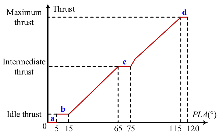
As shown in Figure A1, four planned dead zones in thrust variation are labeled as a through d, corresponding to the engine’s shutdown, idle, intermediate, and full afterburning states, respectively. For the remaining zones, the throttle-to-thrust relationship must ensure high linearity. Additionally, to ensure the pilot can perceive the activation of the afterburning state, a rapid increase in thrust is essential when the afterburning state is engaged.
Figure A1.
Desired throttle-to-thrust relationship.
Appendix A.2. Effectiveness of Dual-Model Training in SSNN
Taking the estimation of the intermediate thrust as an example, the performance comparison and error statistics of different training modes for SSNN 1# are shown in Figure A2 and Table A1, respectively. Compared to single-model training, dual-model training significantly improves the performance of SSNN 1#.
Figure A2.
Comparison of different training modes for SSNN 1#. (a) Relative error. (b) Absolute error.
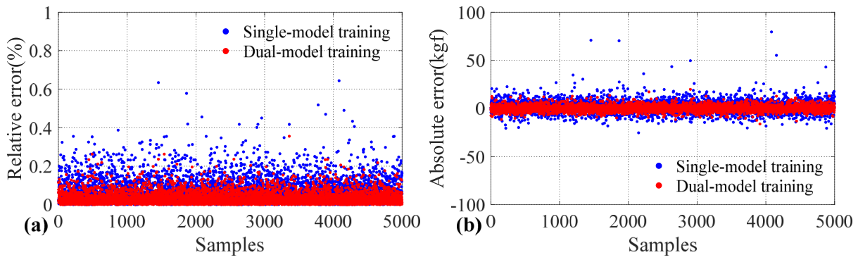
Table A1.
Error statistics of different training modes for SSNN 1#.
Appendix A.3. Variant of SSNN: Introduction of the Binary Neural Network
In addition to the impact of the online update on real-time performance, it is essential to consider the encroachment of the proposed RTCS on existing hardware resources. To meet the demands of future embedded applications, it is also crucial to conserve memory space and enhance offline computational speed. To achieve this, we propose replacing the first network in the SSNN, switching from the original FCNN to the BNN. Specifically, the weights and activations of this network are constrained to 1-bit, leading to substantial memory savings. Meanwhile, floating-point multiplication operations are replaced by XNOR and bitcount operations, which further improve computational speed [44,45]. Within the SSNN architecture, the second network also compensates for the accuracy loss caused by the binarization process.
During forward propagation, the sign function is commonly used for binarization. Assuming x represents the independent variable of the function, it is expressed as follows.
Since the sign function is not differentiable, the straight-through estimator technique is used to compute the gradient during backward propagation [46], which is defined as follows.
where the clip function is used to effectively prevent large full-precision parameters during the update process, thereby ensuring that the binarized parameters can be continuously updated.
Moreover, to improve the performance of the BNN, the ReLU function is replaced with the PReLU function as the activation function, as shown below.
where a denotes the parameter to be learned.
The basic settings of this new SSNN are presented in Table A2. Taking the estima-tion of the intermediate thrust as an example, the performance at engine initial use and during the first 50 h are shown in Figure A3 and Figure A4, respectively. The corresponding error statistics are given in Table A3 and Table A4, respectively. The sample index in Figure A3 is used only to display pointwise prediction errors over the testing samples and does not represent a physical or temporal variable. The quantitative error distribution is summarized by the maximum, mean, and standard deviation values in Table A3. Compared to the original SSNN, the new SSNN also achieves satisfactory performance. At engine initial use, New SSNN 1# achieves a maximum relative error of 0.83%, as shown in Table A3. During the first 50 h of engine operation, its maximum relative error is 3.09%, as shown in Table A4. These two values correspond to different evaluation cases and should be interpreted separately. Because New SSNN 1# has a larger second-network configuration than New SSNN 2#, it is expected to provide smaller errors in some cases. Therefore, this comparison should be interpreted as a model-capacity/accuracy trade-off rather than as evidence that one configuration is universally superior. However, whether the new SSNN can truly meet our expectations remains to be verified by future embedded applications on the engine controllers.
Figure A3.
Pointwise prediction errors of the new SSNN at engine initial use over the testing samples. (a) Relative error. (b) Absolute error.
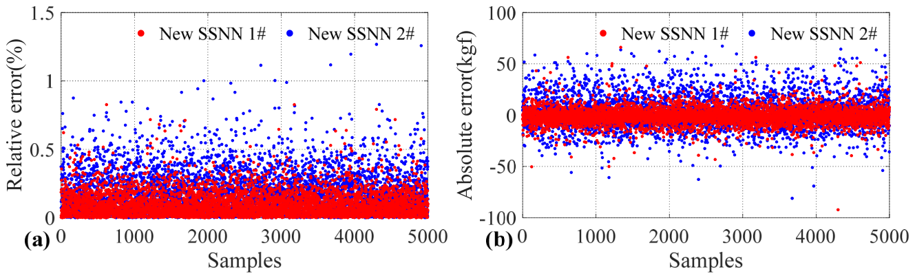
Figure A4.
Performance of the new SSNN during the first 50 h. (a) Relative error. (b) Absolute error.
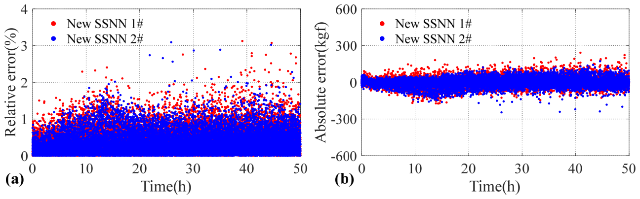
Table A2.
Basic settings of the new SSNN. Note: The numbers in parentheses indicate the number of neurons in each hidden layer.
Table A3.
Error statistics of the new SSNN at engine initial use.
Table A4.
Error statistics of the new SSNN during the first 50 h.
References
- Zhao, H.; Liao, Z.; Liu, J.; Li, M.; Liu, W.; Wang, L.; Song, Z. A highly robust thrust estimation method with dissimilar redundancy framework for gas turbine engine. Energy 2022, 245, 123255. [Google Scholar] [CrossRef] [Scilit]
- Balli, O. Thermodynamic, thermoenvironmental and thermoeconomic analyses of piston-prop engines (PPEs) for landing and take-off (LTO) flight phases. Energy 2022, 250, 123725. [Google Scholar]
- Aygun, H.; Caliskan, H. Environmental and enviroeconomic analyses of two different turbofan engine families considering landing and take-off (LTO) cycle and global warming potential (GWP) approach. Energy Convers. Manag. 2021, 248, 114797. [Google Scholar] [CrossRef] [Scilit]
- Zhuang, L.; Xu, G.; Liu, Q.; Li, M.; Dong, B.; Wen, J. Superiority analysis of the cooled cooling air technology for low bypass ratio aero-engine under typical flight mission. Energy Convers. Manag. 2022, 259, 115510. [Google Scholar] [CrossRef] [Scilit]
- Zhang, Z.; Peng, Y.; Wei, X.; Li, L.; Wang, Y.; Liu, X. Research on longitudinal dynamics safety boundary of carrier-based aircraft arresting. Aerosp. Sci. Technol. 2022, 130, 107864. [Google Scholar] [CrossRef] [Scilit]
- Xiao, H.; Zhen, Z.; Xue, Y. Fault-tolerant attitude tracking control for carrier-based aircraft using RBFNN-based adaptive second-order sliding mode control. Aerosp. Sci. Technol. 2023, 139, 108408. [Google Scholar]
- Zhou, X.; Lu, F.; Zhou, W.; Huang, J. An improved multivariable generalized predictive control algorithm for direct performance control of gas turbine engine. Aerosp. Sci. Technol. 2020, 99, 105576. [Google Scholar] [CrossRef] [Scilit]
- Lv, C.; Chang, J.; Bao, W.; Yu, D. Recent research progress on airbreathing aero-engine control algorithm. Propuls. Power Res. 2022, 11, 1–57. [Google Scholar] [CrossRef] [Scilit]
- Henriksson, M.; Gronstedt, T.; Breitholtz, C. Model-based on-board turbofan thrust estimation. Control Eng. Pract. 2011, 19, 602–610. [Google Scholar]
- Zhu, Y.; Huang, J.; Pan, M.; Zhou, W. Direct thrust control for multivariable turbofan engine based on affine linear parameter-varying approach. Chin. J. Aeronaut. 2022, 35, 125–136. [Google Scholar] [CrossRef] [Scilit]
- Pang, S.; Jafari, S.; Nikolaidis, T.; Li, Q. Reduced-dimensional MPC controller for direct thrust control. Chin. J. Aeronaut. 2022, 35, 66–81. [Google Scholar] [CrossRef] [Scilit]
- Zhao, H.; Zhai, X.; Liao, Z.; Li, Z.; Song, Z. Gas turbine thrust estimation in sensor drift scenarios using a three-stage multi-target domain adaptation method. Energy 2025, 314, 134104. [Google Scholar]
- Zhao, Y.; Li, Z.; Hu, Q. A size-transferring radial basis function network for aero-engine thrust estimation. Eng. Appl. Artif. Intell. 2020, 87, 103253. [Google Scholar]
- Li, Z.-Q.; Zhao, Y.-P.; Cai, Z.-Y.; Xi, P.-P.; Pan, Y.-T.; Huang, G.; Zhang, T.-H. A proposed self-organizing radial basis function network for aero-engine thrust estimation. Aerosp. Sci. Technol. 2019, 87, 167–177. [Google Scholar]
- Zhao, Y.; Hu, Q.; Xu, J.; Li, B.; Huang, G.; Pan, Y. A robust extreme learning machine for modeling a small-scale turbojet engine. Appl. Energy 2018, 218, 22–35. [Google Scholar] [CrossRef] [Scilit]
- Litt, J.S.; Sowers, T.S. Evaluation of Outer Loop Retrofit Architecture for Intelligent Turbofan Engine Thrust Control; NASA/TM-2006-214460; NASA: Washington, DC, USA, 2006.
- Litt, J.S.; Turso, J.A.; Shah, N.; Sowers, T.S.; Owen, A.K. A Demonstration of a Retrofit Architecture for Intelligent Control and Diagnostics of a Turbofan Engine; NASA/TM-2005-214019; NASA: Washington, DC, USA, 2005.
- Litt, J.S.; Parker, K.I.; Chatterjee, S. Adaptive Gas Turbine Engine Control for Deterioration Compensation Due to Aging; NASA/TM-2003-212607; NASA: Washington, DC, USA, 2003.
- Chatterjee, S.; Litt, J.S. Online Model Parameter Estimation of Jet Engine Degradation for Autonomous Propulsion Control; NASA/TM-2003-212608; NASA: Washington, DC, USA, 2003.
- Litt, J.S.; Sowers, T.S.; Garg, S. A Retro-Fit Control Architecture to Maintain Engine Performance with Usage; NASA/TM-2007-214977; NASA: Washington, DC, USA, 2007.
- Yan, Z.; Qiu, X.; Huang, J.; Lu, F. Neural network control of aircraft engine thrust degradation mitigation. J. Aerosp. Power 2020, 35, 844–854. [Google Scholar]
- Zhao, K.; Li, D.; Li, B. Research on performance recovery for engine performance deterioration. J. Propuls. Technol. 2015, 36, 1560–1566. [Google Scholar]
- Li, Y.; Li, Q.; Huang, X.; Zhao, Y. Performance deterioration mitigation control of aero-engine. J. Aerosp. Power 2012, 27, 930–936. [Google Scholar]
- Zhou, X.; Huang, J.; Lu, F.; Zhou, W.; Liu, P. A novel compound fault-tolerant method based on online sequential extreme learning machine with cycle reservoir for turbofan engine direct thrust control. Aerosp. Sci. Technol. 2023, 132, 108059. [Google Scholar]
- Chen, Q.; Sheng, H.; Zhang, T. A novel direct performance adaptive control of aero-engine using subspace-based improved model predictive control. Aerosp. Sci. Technol. 2022, 128, 107760. [Google Scholar]
- Ma, J.; Chang, J.; Ma, J.; Bao, W.; Yu, D. Mathematical modeling and characteristic analysis for over-under turbine based combined cycle engine. Acta Astronaut. 2018, 148, 141–152. [Google Scholar] [CrossRef] [Scilit]
- Wei, Z.; Zhang, S.; Jafari, S.; Nikolaidis, T. Gas turbine aero-engines real time on-board modelling: A review, research challenges, and exploring the future. Prog. Aerosp. Sci. 2020, 121, 100693. [Google Scholar]
- Imani, A.; Montazeri-Gh, M. Improvement of Min-Max limit protection in aircraft engine control: An LMI approach. Aerosp. Sci. Technol. 2017, 68, 214–222. [Google Scholar]
- Pang, S.; Jafari, S.; Nikolaidis, T.; Li, Q. A novel model-based multivariable framework for aircraft gas turbine engine limit protection control. Chin. J. Aeronaut. 2021, 34, 57–72. [Google Scholar] [CrossRef] [Scilit]
- Lu, F.; Wu, J.; Huang, J.; Qiu, X. Aircraft engine degradation prognostics based on logistic regression and novel OS-ELM algorithm. Aerosp. Sci. Technol. 2019, 84, 661–671. [Google Scholar] [CrossRef] [Scilit]
- Zhu, Y.; Pan, M.; Zhou, W.; Huang, J. Intelligent direct thrust control for multivariable turbofan engine based on reinforcement and deep learning methods. Aerosp. Sci. Technol. 2022, 131, 107972. [Google Scholar] [CrossRef] [Scilit]
- Sallee, G.P. Performance deterioration based on existing (historical) data. In JT9D Jet Engine Diagnostics Program; NASA: Washington, DC, USA, 1978. [Google Scholar]
- Jin, P.; Zhou, X.; Wang, C.; Huang, J.; Zhou, W.; Lu, F. A novel distributed Kalman filtering for health state recognition of aero-engine components in networked control systems. Nonlinear Dyn. 2023, 111, 2571–2589. [Google Scholar]
- Zheng, J.; Chang, J.; Ma, J.; Yu, D. Performance uncertainty propagation analysis for control-oriented model of a turbine-based combined cycle engine. Acta Astronaut. 2018, 153, 39–49. [Google Scholar]
- Lu, F.; Wu, J.; Huang, J.; Qiu, X. Restricted-Boltzmann-based extreme learning machine for gas path fault diagnosis of turbofan engine. IEEE Trans. Ind. Inform. 2020, 16, 959–968. [Google Scholar]
- Wang, J.; Guo, Y.; Zhou, K.; Xia, J.; Li, Y.; Zhao, P.; Dai, Y. Design and performance analysis of compressor and turbine in supercritical CO2 power cycle based on system-component coupled optimization. Energy Convers. Manag. 2020, 221, 113179. [Google Scholar] [CrossRef] [Scilit]
- Lin, A.; Liu, G.; Wang, X.; Feng, Q. Comprehensive evaluations on performance and energy consumption of pre-swirl rotor-stator system in gas turbine engines. Energy Convers. Manag. 2021, 244, 114440. [Google Scholar]
- Feng, H.; Liu, B.; Xu, M.; Li, M.; Song, Z. Model-based deduction learning control: A novel method for optimizing gas turbine engine afterburner transient. Energy 2024, 292, 130512. [Google Scholar] [CrossRef] [Scilit]
- Qin, H.; Gong, R.; Liu, X.; Bai, X.; Song, J.; Sebe, N. Binary neural networks: A survey. Pattern Recognit. 2020, 105, 107281. [Google Scholar] [CrossRef] [Scilit]
- Courbariaux, M.; Bengio, Y.; David, J. BinaryConnect: Training deep neural networks with binary weights during propagations. In Proceedings of the Advances in Neural Information Processing Systems 28 (NIPS 2015), Montreal, QC, Canada, 7–12 December 2015. [Google Scholar]
- Kingma, D.P.; Ba, J.L. Adam: A method for stochastic optimization. arXiv 2014, arXiv:1412.6980. [Google Scholar]
- Ding, S.; Zhao, H.; Zhang, Y.; Xu, X.; Nie, R. Extreme learning machine: Algorithm, theory and applications. Artif. Intell. Rev. 2015, 44, 103–115. [Google Scholar]
- Huang, G.; Zhou, H.; Ding, X.; Zhang, R. Extreme learning machine for regression and multiclass classification. IEEE Trans. Syst. Man. Cybern. Part B-Cybern. 2012, 42, 513–529. [Google Scholar]
- Lin, X.; Zhao, C.; Pan, W. Towards Accurate Binary Convolutional Neural Network. In Proceedings of the Advances in Neural Information Processing Systems 30 (NIPS 2017), Long Beach, CA, USA, 4–9 December 2017. [Google Scholar]
- Rastegari, M.; Ordonez, V.; Redmon, J.; Farhadi, A. XNOR-Net: ImageNet classification using binary convolutional neural networks. In Proceedings of the 14th European Conference, Amsterdam, The Netherlands, 11–14 October 2016. [Google Scholar]
- Liu, Z.; Cheng, K.; Huang, D.; Xing, E.; Shen, Z. Nonuniform-to-uniform quantization: Towards accurate quantization via generalized straight-through estimation. In Proceedings of the IEEE/CVF Conference on Computer Vision and Pattern Recognition (CVPR), New Orleans, LA, USA, 18–24 June 2022. [Google Scholar]
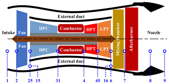
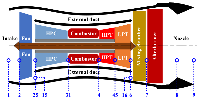
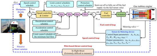
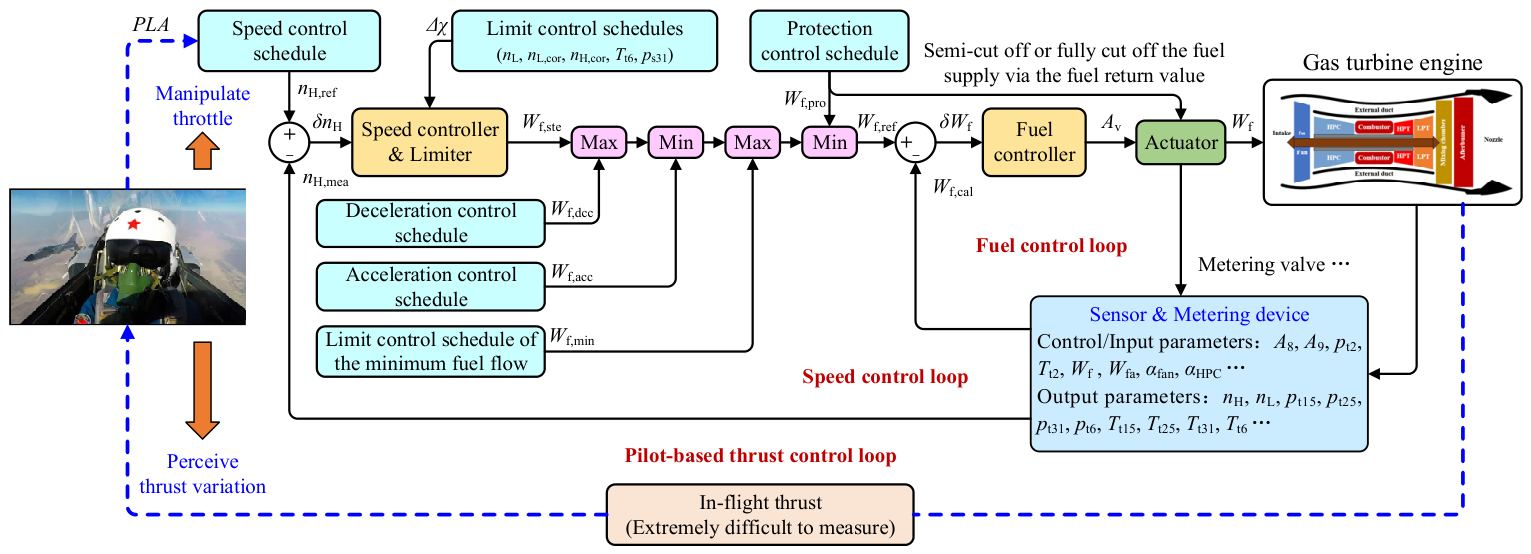
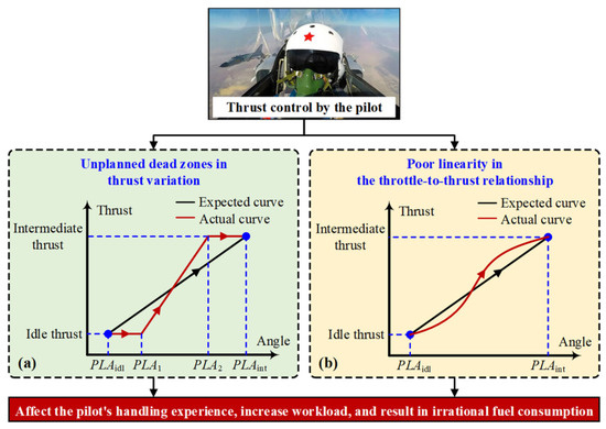
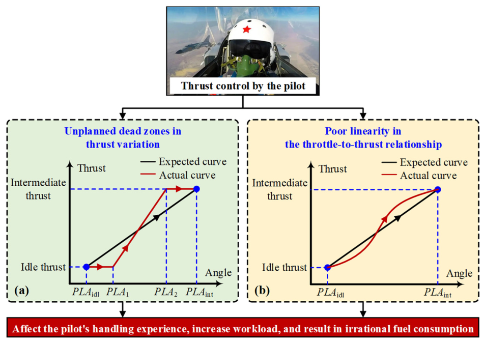
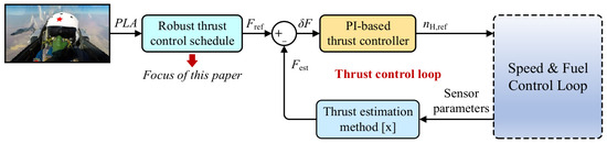
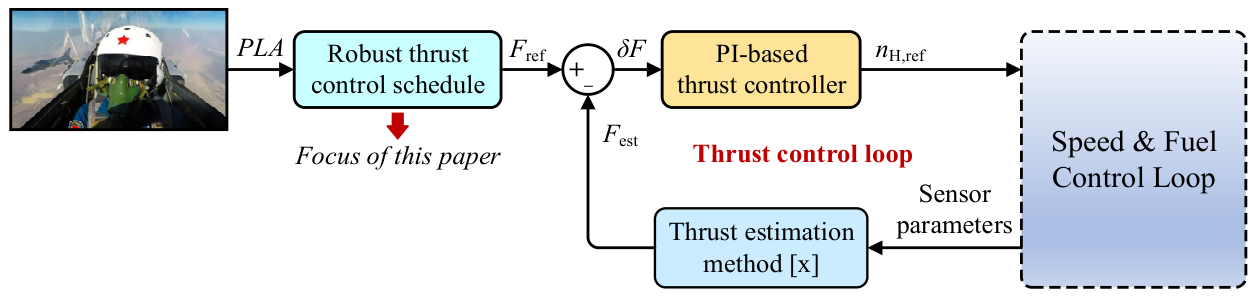
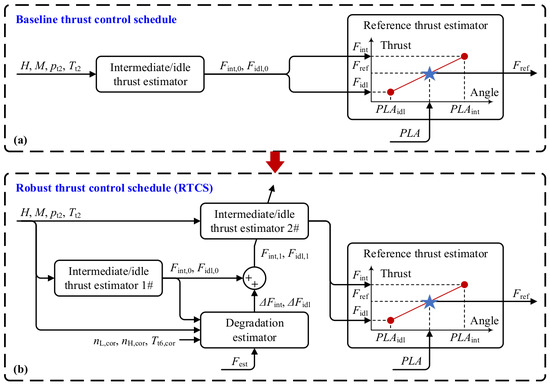
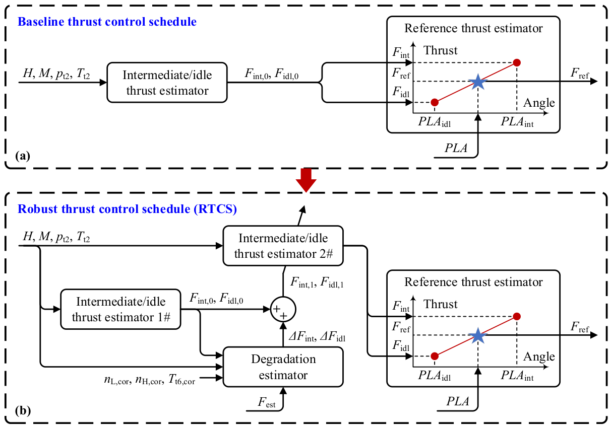
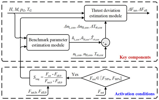
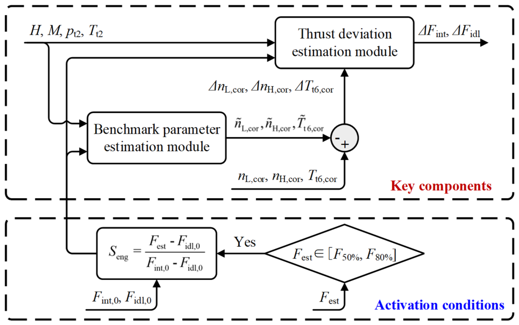
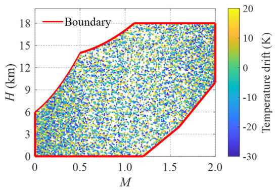
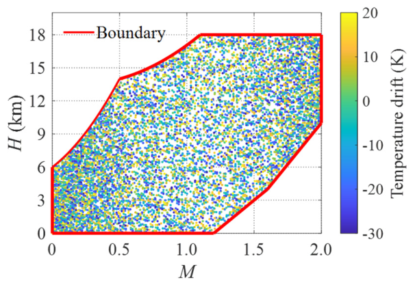
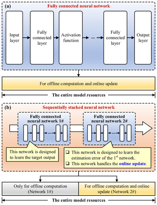
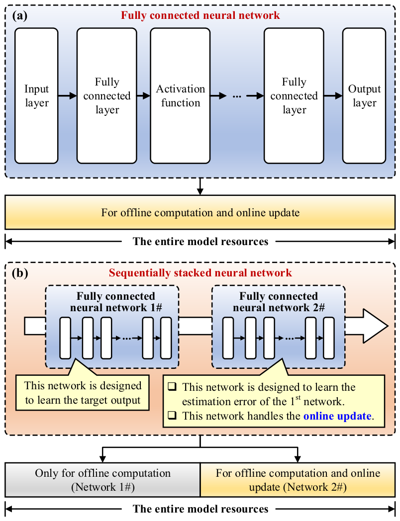
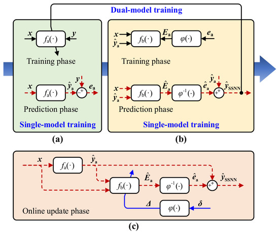
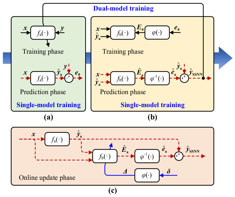
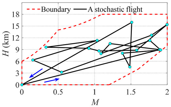
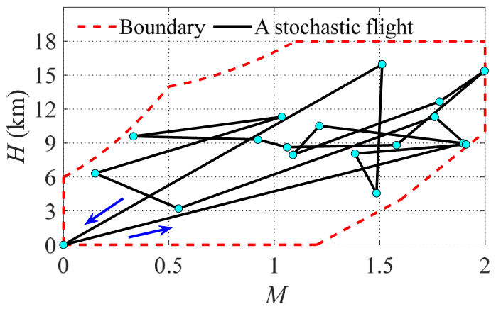
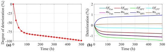
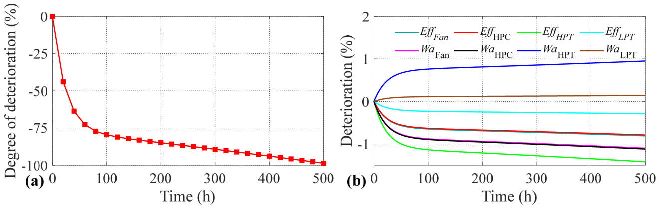
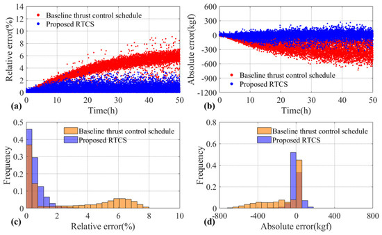
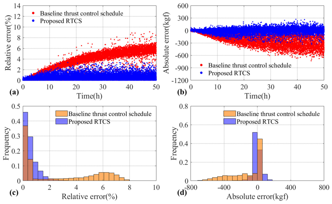
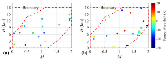
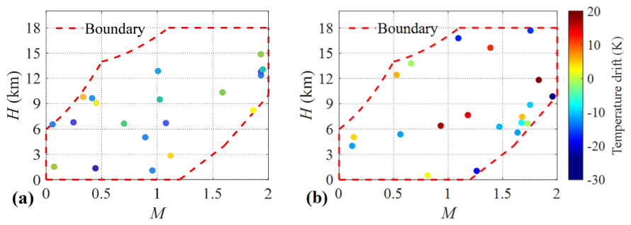
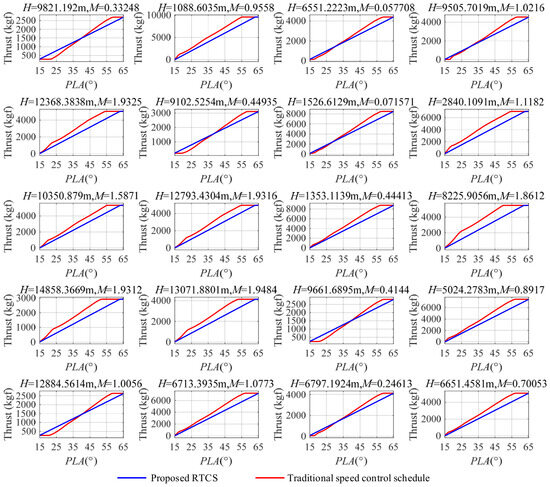
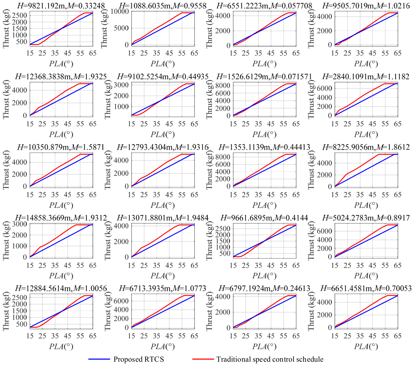
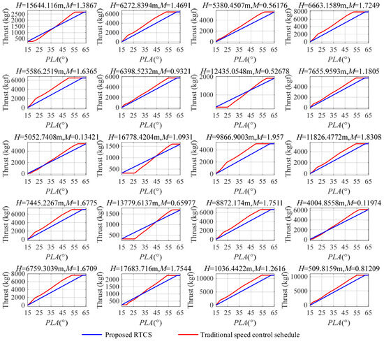
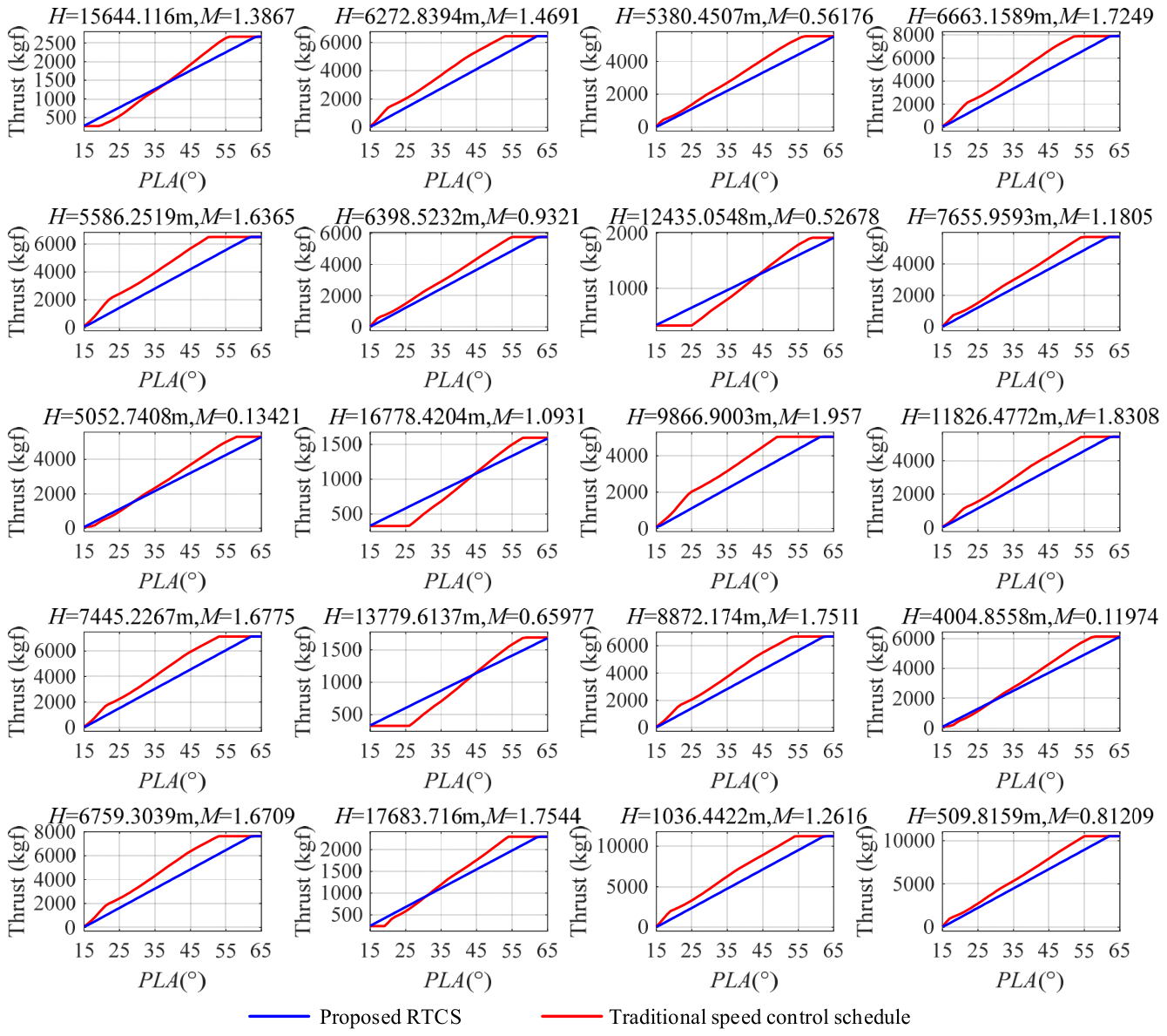
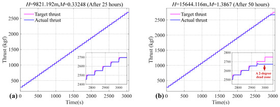
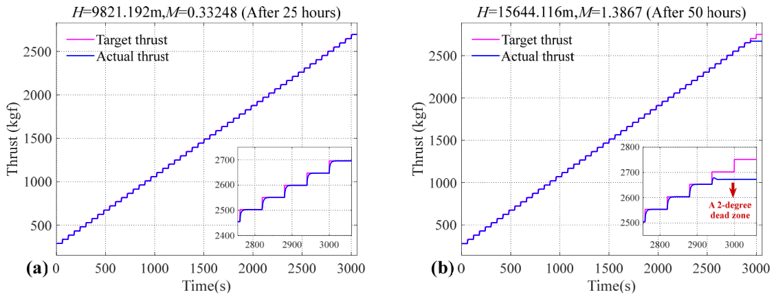
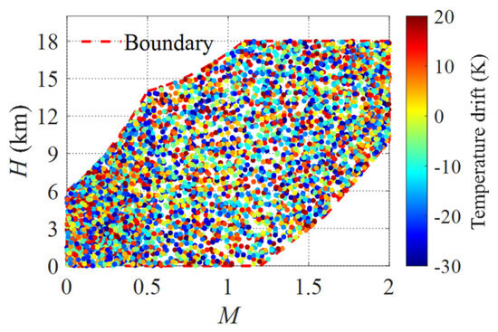
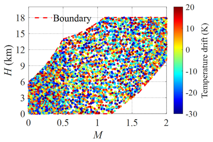
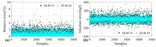
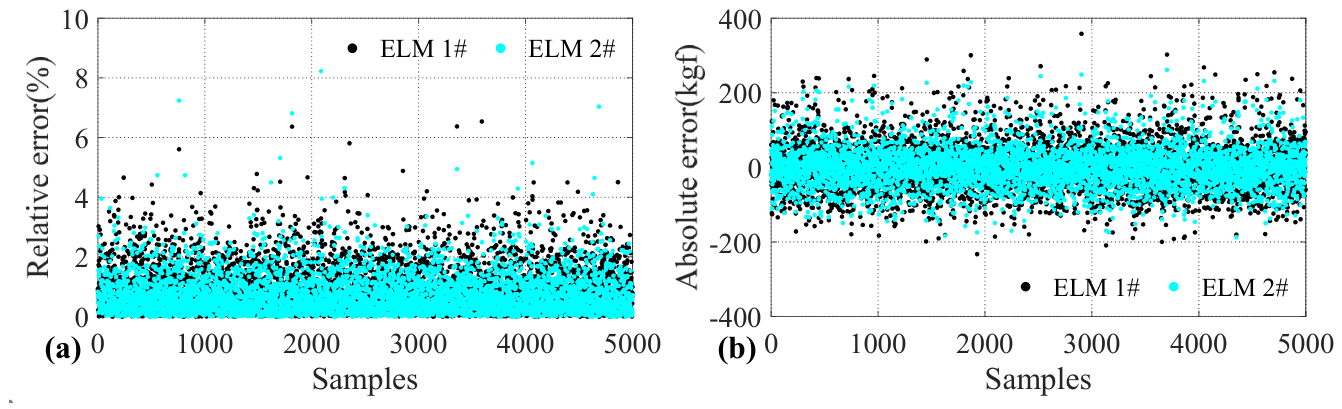
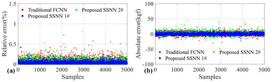
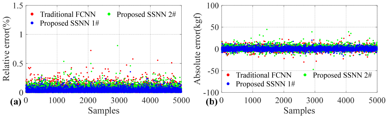
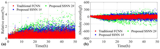
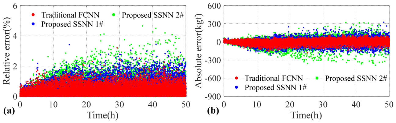
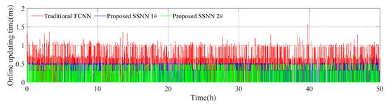
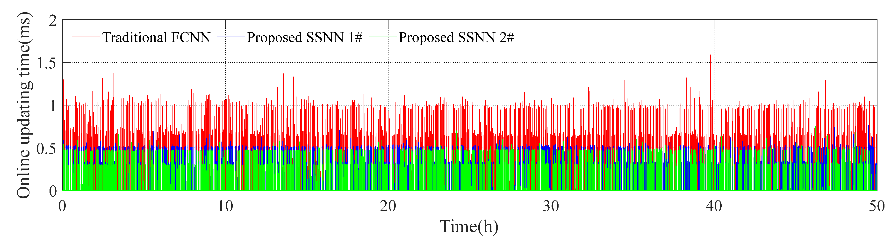
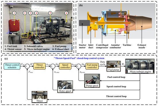
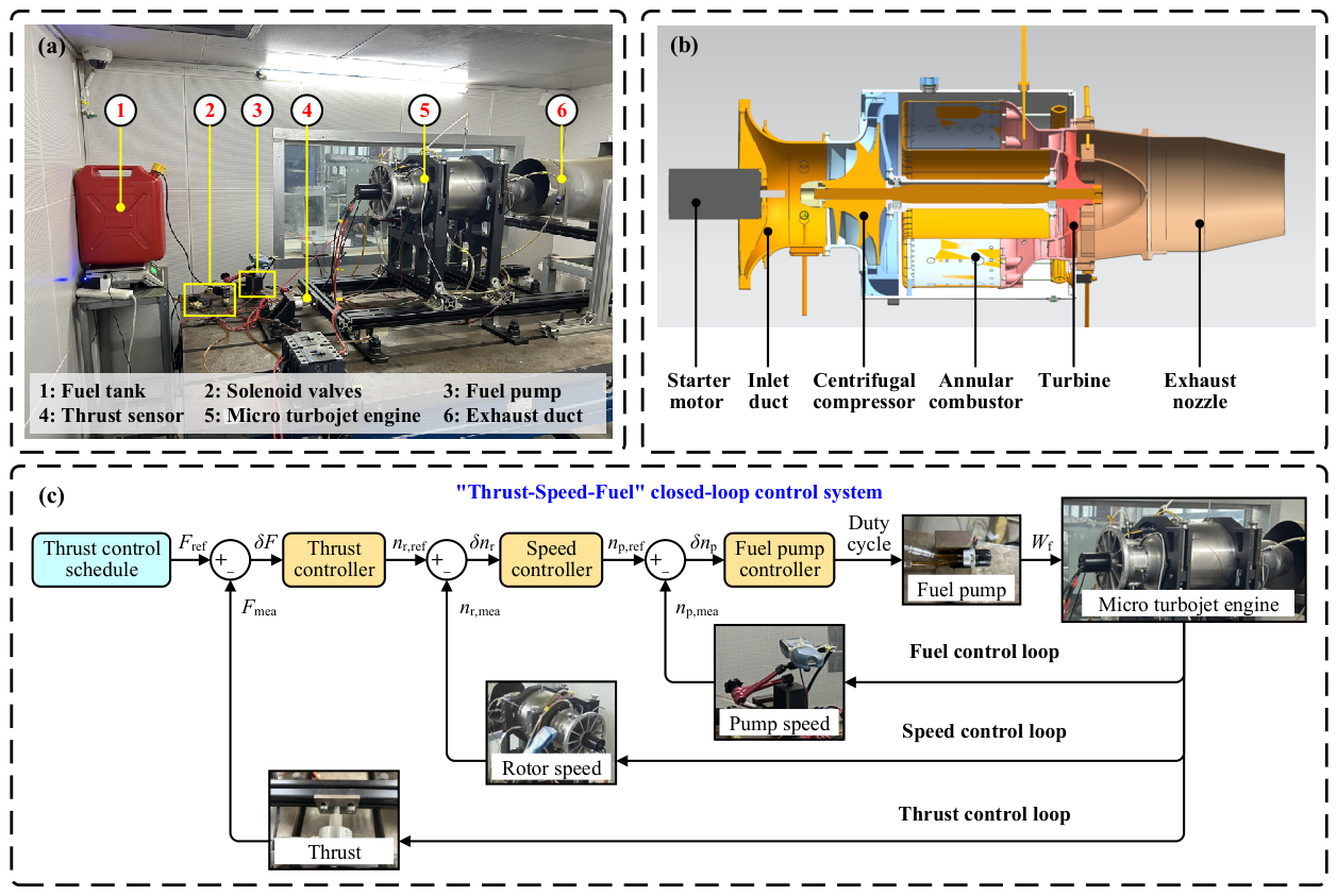
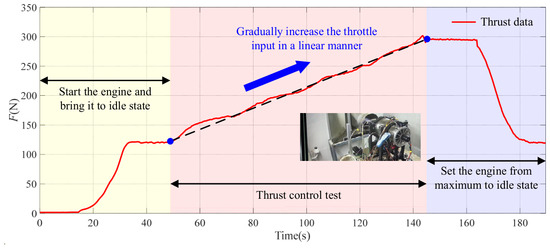
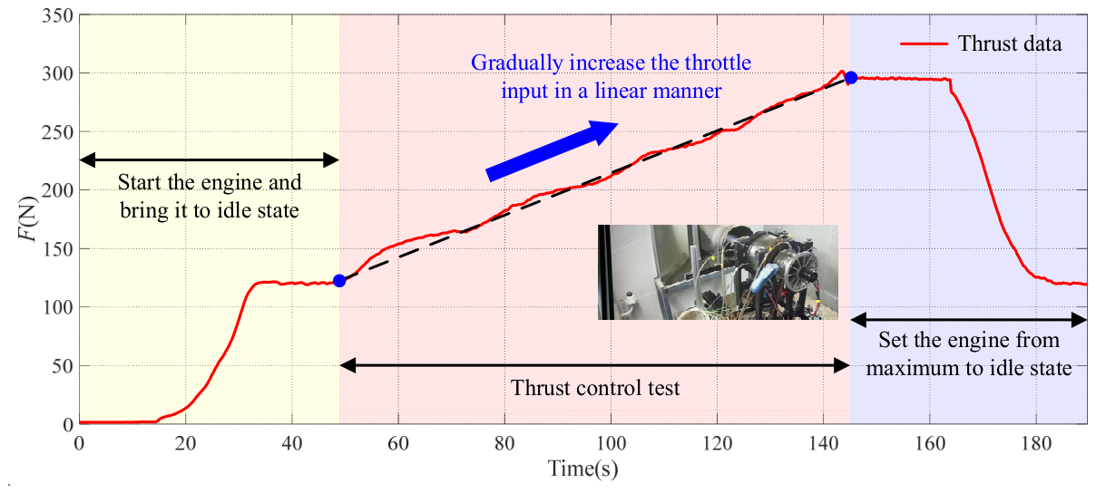

Disclaimer/Publisher’s Note: The statements, opinions and data contained in all publications are solely those of the individual author(s) and contributor(s) and not of MDPI and/or the editor(s). MDPI and/or the editor(s) disclaim responsibility for any injury to people or property resulting from any ideas, methods, instructions or products referred to in the content. |
© 2026 by the authors. Licensee MDPI, Basel, Switzerland. This article is an open access article distributed under the terms and conditions of the Creative Commons Attribution (CC BY) license.