Research on the Parameters Reconstruction Method of Pipe Structures Based on Intelligent Optimization Algorithms

Abstract

Two reconstruction methods for constraint and load parameters of aero-engine pipelines based on intelligent optimization algorithms are proposed in this paper. First, a simplified finite element model (FEM) of the aero-engine pipeline structure is established, and its reliability is validated by comparing simulation data with experimental data. Second, a reconstruction algorithm for spring constraint parameters and pipeline load parameters based on the improved particle swarm optimization (IPSO) algorithm is developed on the MATLAB data analysis and ANSYS simulation platforms, which completes the reconstruction calculation of parameters such as spring constraint stiffness and applied harmonic excitation. For harmonic excitation parameter reconstruction, the maximum error of this algorithm reaches 24.9%, revealing its significant inapplicability to load parameter reconstruction. To solve this problem, a load reconstruction method based on the conjugate gradient method (CGM) is further proposed to achieve accurate reconstruction of pipeline load parameters, which mitigates the large reconstruction error of the IPSO algorithm under working conditions with multiple loads. Under 5% noise interference, the maximum error of the CGM is merely 5.16%. Finally, experimental verification of harmonic excitation amplitude reconstruction is performed using the CGM with lower reconstruction errors. Experimental results indicate that the maximum error is 14.24% for harmonic excitation amplitude reconstruction, which verifies the high applicability of the conjugate gradient algorithm to load reconstruction of aero-engine pipelines.

1. Introduction

Aero-engine pipelines feature complex spatial structures, diverse transmission media, and intricate vibration conditions in service environments. In addition to mechanical vibration loads, the internal pipelines also bear complex fluid dynamic loads caused by oil–gas two-phase flow [1]. Traditional load prediction methods for engines derived from preliminary structural design theories can no longer satisfy the requirements of modern aerospace engineering for accurately obtaining load and constraint information. In aerospace engineering, the adverse effects of vibrational loads on aero-engine pipeline structures, particularly thin-walled pipelines, must be taken into consideration. Long-term pipeline vibration will trigger severe fretting wear at the contact position of pipe ferrules, which eventually leads to irreversible sealing failure of aircraft hydraulic pipeline joints; such vibration-induced fretting fatigue failure has been verified through accelerated vibration tests [2]. Vibration-induced fatigue at stress-concentrated regions is a critical concern for high-pressure pipeline fittings in aerospace propulsion systems (e.g., liquid rocket engine pipelines and aero-engine pipelines), and dynamic vibration loads are the primary cause of fatigue failure in such pipeline components [3]. Complete measured vibration load spectra serve as essential input for mission-synthesis accelerated fatigue tests of aviation aluminum alloy components with segmented S-N curves, and the precision of fatigue evaluation results directly depends on the accuracy of acquired dynamic load data [4]. The acquired load parameter information supports structural health monitoring, dynamic response analysis, and reliability analysis of pipelines [5,6], which further reduces costs related to the design, manufacturing, operation, and maintenance of engineering structures. For aero-engine pipelines with increasingly refined structural details, traditional methods for estimating load and constraint parameters are far from adequate. If load and constraint information can be inversely reconstructed from pipeline structural response parameters, a novel technical approach will be developed to obtain the load conditions and constraint states of in-service aero-engine pipeline structures. The technology that indirectly acquires load and constraint parameters of internal aero-engine pipeline systems from pipeline response information is defined as reconstruction technology.

Load and constraint parameter reconstruction techniques play a crucial role in structural vibration mechanics research, and numerous reconstruction methods for various loads and constraint parameters have been developed by scholars worldwide. M. Hansen [7] discovered ill-conditioned coefficient matrices near the natural frequency range of structures during the inversion of frequency response functions. Prawin and Rao [8] proposed a load reconstruction algorithm based on dynamic principal component analysis (DPCA) that further simplifies the model updating process of structural finite element models. Miao et al. [9] established reconstruction equations for system load identification based on Green’s kernel function. Combined numerical and experimental results verified the accuracy of truncated singular value decomposition (TSVD) regularization in solving continuous loads. Chen [10] put forward a dynamic load identification and reconstruction method for satellite rocket interfaces based on back propagation (BP) neural networks. Satellite acceleration responses were obtained through simulation analyses and experiments. By comparison with actual satellite acceleration samples, the proposed method realizes the identification and reconstruction of satellite acceleration excitations using measured acceleration responses.

Liu et al. [11] developed an adaptive weak magnetic signal reconstruction method based on multi-scale signal decomposition and an improved sparrow search algorithm. This method effectively suppresses complex noise interference in pipeline stress detection and significantly improves the reconstruction accuracy of weak magnetic signals and the reliability of stress inversion results. Zhu et al. [12] adopted a genetic-algorithm-optimized variational mode decomposition method to denoise negative pressure wave signals generated by pipeline leakage. It effectively eliminates complex noise interference and greatly enhances pipeline leakage signal quality and leakage localization accuracy. Zhang et al. [13] realized nonlinear state reconstruction of hydrogen transporting pipelines via physics informed neural networks (PINNs), which can accurately characterize the spatiotemporal evolution of multi-physical parameters inside pipelines with limited measured data. Han et al. [14] proposed a neural implicit reconstruction method for spacecraft pose estimation without offline prior information. This method enables parallel implementation of pose tracking, neural target reconstruction and target reference frame estimation. Experimental results demonstrate that the method can adapt to multiple types of targets without prior information and effectively cope with complex on-orbit conditions, including large scale motion, specular highlights and thin-walled structures. Gao et al. [15] presented an inversion scheme for load and constraint reconstruction of pipeline structures. A forward stochastic vibration simulation model was constructed, and a multi-step inversion strategy was adopted to solve unknown load and constraint parameters. A pipeline vibration test system was built for validation, and the method can realize global vibration evaluation of pipelines based on limited vibration monitoring data.

To address the defect post-processing detection limitation of traditional X-ray computed tomography (CT) for subsea pipelines, Christensen et al. [16] proposed a Bayesian CT reconstruction method with built-in defect detection. Structural and defect images are separated and synchronously inversely reconstructed. Experimental verifications prove that this method can quantify the uncertainty of defect detection while ensuring reconstruction quality. Aiming at the challenges of hyperbolic feature extraction and parameter fitting for underground targets in ground penetrating radar (GPR) B-scan images, Jin et al. [17] proposed the GPR Former model. Based on the Transformer network, this model directly regresses hyperbolic parameters and optimizes fitting results using analytical solutions under symmetric constraints, thus enabling efficient automatic detection and parameter reconstruction of underground pipelines. Wang et al. [18] constructed a visual detection system based on electrical resistance tomography (ERT) and proposed an adaptive finite element mesh spatial second-order total variation iterative reconstruction algorithm. Simulations and experiments indicate that this algorithm can greatly improve reconstruction efficiency and accuracy and achieve real-time visual monitoring of pipeline inner-wall scaling. To tackle the problems of short detection distance and large positioning error in acoustic leakage detection of buried pipelines, Zhou et al. [19] proposed an adaptive acoustic leakage localization method based on transient-optimized statistical analysis. Transient components of reconstructed signals are decomposed, and maximum correlated kurtosis deconvolution is optimized under minimum envelope entropy constraints. Leakage point localization is completed via time delay probability weighting, and the proposed method outperforms existing mainstream approaches. Xu X et al. [20] improved the traditional particle swarm optimization algorithm according to the “ill-posed problem” in inverse problem processing, and proposed the method of reconstructing load parameters using the improved particle swarm optimization algorithm (GAPSO).

However, most existing reconstruction methods for load and constraint parameters mainly focus on uniformly distributed loads acting on large-scale components or structures. For aero-engine pipeline systems applied in the aerospace industry, they are primarily subjected to static loads, impact loads, harmonic excitations and random excitations, where loads and constraints act on small local regions. Therefore, it is of great significance to further develop reconstruction technologies targeting load and constraint parameters of aero-engine pipeline systems, so as to accurately obtain relevant load and constraint information. Reliable multi-axial load data provides core input for fatigue life evaluation of notched pipeline structures under a random vibration environment [21]. This ensures the stable operation of pipeline systems and provides comprehensive excitation and constraint data for health monitoring of similar aero-engine pipelines.

2. Basic Theory of Pipeline Structural Parameter Reconstruction

2.1. Fundamental Theory for Forward Problem Analysis of Pipelines

Pipeline structural dynamics focuses on the global and local response characteristics of tubular structures under boundary constraints and dynamic excitations, mainly covering displacement, stress and strain analysis. For complex spatially distributed aero-engine pipeline systems, the finite element method (FEM) serves as an efficient and widely adopted dynamic analysis tool [22]. Benefiting from the special geometric characteristics of pipe structures, dedicated pipe elements can be utilized for numerical simulation, which enables modeling of intricate pipeline assemblies with only a small quantity of discrete elements. Based on fundamental finite element theory, the displacement response of arbitrary structural nodes under dynamic vibration excitations complies with the linear vibration equilibrium equation as follows:

$$\left[M\right]\left\{\ddot{x}\right\}+\left[C\right]\left\{\dot{x}\right\}+\left[K\right]\left\{x\right\}=\left\{F\left(t\right)\right\}$$

(1)

In Equation (1), M is the mass matrix of the overall structural system, C denotes the damping matrix, K represents the stiffness matrix, and $F\left(t\right)$ stands for the characteristic parameters of force excitation. $\ddot{x}$, $\dot{x}$ and x are the acceleration vector, velocity vector and displacement vector of unconstrained nodes on the pipeline, respectively.

When the pipeline structure is excited by sinusoidal loads, it vibrates at the identical frequency irrespective of variations in the input excitation frequency. Under periodic excitation, the structural vibration equation is written as

$$\left[M\right]\left\{\ddot{X}\right\}+\left[C\right]\left\{\dot{X}\right\}+\left[K\right]\left\{X\right\}=\left\{F\right\}sin2\pi ft$$

(2)

In Equation (2), F is the amplitude of harmonic excitation and f is the frequency of the input excitation force. The displacement response of the structure under continuous harmonic excitation is given by

$$\left\{X\right\}=\left\{A\right\}sin(2\pi ft+\phi )$$

(3)

In Equation (3), A represents the displacement amplitude vector, which is associated with the structural natural frequency, excitation frequency and system damping. $\phi$ refers to the phase angle by which the displacement lags behind the excitation applied to the structure. The structural response under harmonic vibration can be directly acquired using the step-by-step integration method based on Equation (2), or solved by the spectrum superposition method with natural frequencies and mode shapes.

2.2. Construction of Objective Function

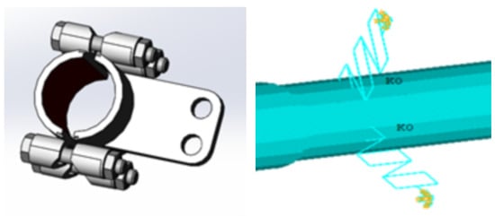
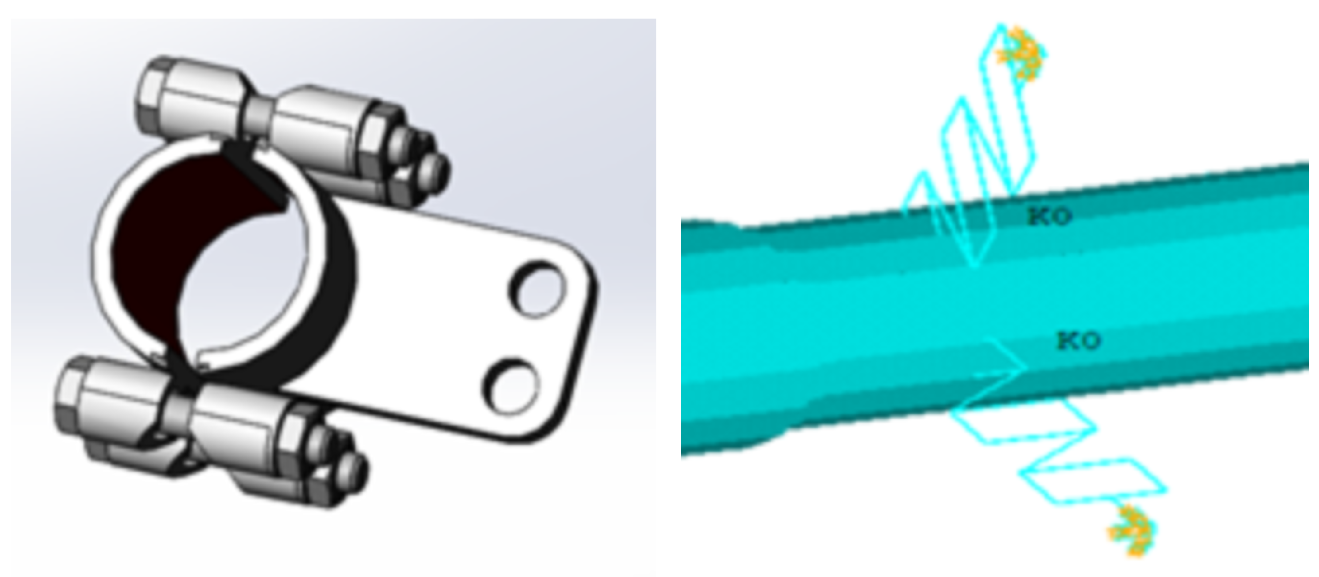
Load parameter reconstruction of aero-engine pipelines is critical for indirectly obtaining load information applied to pipelines and further determining the overall vibration deformation of aero-engine pipeline systems. In practical aero-engine pipeline systems, brackets and hoop clamps are widely used for fixing and supporting pipelines, which mainly improve the global stiffness and mitigate vibration of the pipeline system. Such supporting components are generally equivalent to spring--damping structures. As illustrated in Figure 1, the spring element COMBIN14 with local damping is adopted in numerical simulations to model hoop clamps in pipelines. Accordingly, before load reconstruction, the stiffness parameters of single-spring constraint elements in the pipeline structure need to be identified first to characterize the constraint state of the whole pipeline system, which provides a basis for subsequent pipeline load parameter reconstruction.

Figure 1. Model diagram of pipeline hoop clamp.

For the reconstruction of constraint or load parameters of aero-engine pipelines, the excitation acting on the pipeline structure exhibits a linear relationship with its displacement response, and displacement is also linearly related to strain. Therefore, load and strain can be regarded as linearly correlated [23], which is mathematically expressed as

$$\left[Q\right]·\left[C\right]=\left[F\right]$$

(4)

In the formula, Q represents the strain or displacement matrix, boldsymbol C is the correlation matrix, and F denotes the load matrix. The parameter reconstruction problem of pipeline systems can be converted into an optimization problem. Structural characteristic response parameters under given load and constraint conditions are obtained by finite element simulation analysis, and the residual function between such simulated parameters and measured parameters of the real structure is defined as the objective function for the optimization problem.

$$\epsilon \left(c\right)={\displaystyle \sum _{m=1}^M}{\left|Z_m\left(c\right)-Z_m^{obs}\right|}^2$$

(5)

In this equation, c denotes the characteristic parameter vector of unknown system loads, which can be displacement or strain data at measurement points; $Z_m^{obs}$ represents the real-world characteristic parameters or experimental measurements at structural monitoring points; $Z_m\left(c\right)$ refers to the characteristic parameters obtained from numerical simulation during algorithm iteration. In the reconstruction calculation, $Z_m\left(c\right)$ gradually approaches the true experimental measurements as constraint or load characteristic parameters are updated. After constraint or load characteristic parameters are revised via the inverse-problem algorithm, $Z_m\left(c\right)$ can be calculated by solving the forward vibration problem.

2.3. Optimization Principle of Improved Particle Swarm Optimization Algorithm

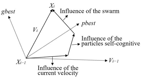
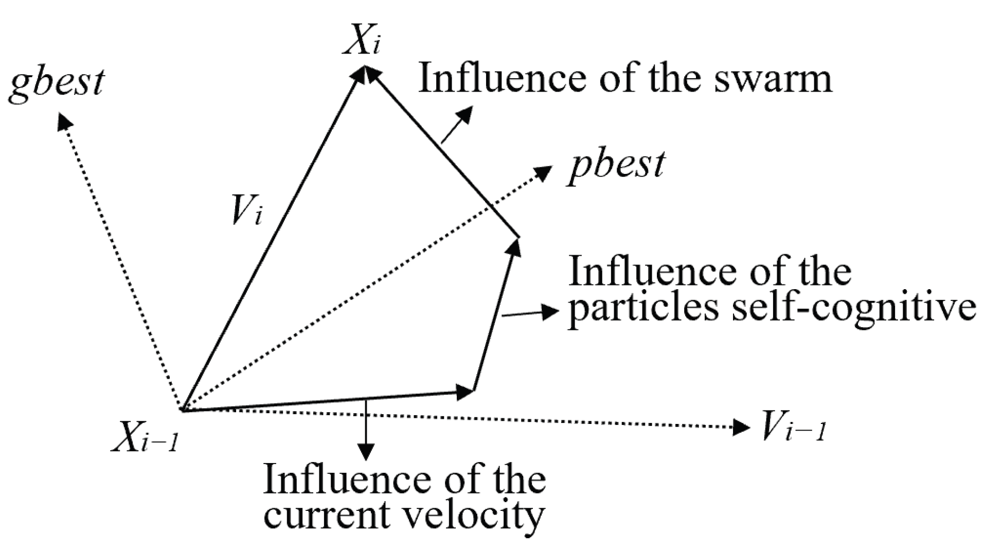
Particle swarm optimization (PSO) is a bio-inspired algorithm that seeks the optimal solution within the feasible solution domain through iterative optimization [24]. In the PSO algorithm, the final position of each particle represents the optimal solution, and the optimization level of particle positions is determined by particle velocity. A schematic diagram of particle position updating is shown in Figure 2.

Figure 2. Schematic diagram of particle position update.

Assume that there are N particles in a population. Let $X_i=(x_1,x_2,\dots ,x_n)$ represent the position of each particle at the i-th iteration, and $V_i=(v_1,v_2,\dots ,v_n)$ represent its velocity at the i-th iteration. $pbest$ denotes the personal best solution of an individual particle in its search history, while $gbest$ refers to the global best solution of the entire particle swarm at the current iteration. The update formulas for particle velocity and position at the i-th iteration are as follows:

$$\begin{array}{c}{V}_i=V_{i-1}\times W+C_1\times rand1\times \left(pbest-X_{i-1}\right)+C_2\times rand2\times \left(gbest-X_{i-1}\right)\end{array}$$

(6)

$$\begin{array}{c}{X}_i=X_{i-1}+V_i\end{array}$$

(7)

where W is the inertia weight of velocity and $C_1$, $C_2$ are acceleration coefficients (also known as learning factors). Specifically, $C_1$ is the self-cognitive learning factor and $C_2$ is the social learning factor. $rand1$ and $rand2$ are random numbers uniformly generated in the range of [0,1]. In the standard particle swarm optimization algorithm, the inertia weight W is generally set to 0.9, and the learning factors $C_1$ and $C_2$ are commonly taken as 2.

2.3.1. Improvement of Inertia Weight

The standard particle swarm optimization (PSO) algorithm tends to converge prematurely and fall into local optima. To meet the requirements of load and constraint parameter reconstruction for aero-engine pipelines, the inertia weight W is improved in this study. A novel definition of inertia weight is adopted such that W decreases linearly with the increase in iteration number, as expressed in Equation (8). This enables the PSO algorithm to perform global search at the initial stage and gradually shift to local exploitation, thereby refining solutions in local regions and improving overall algorithm performance.

$$W=W_{max}-(W_{max}-W_{min})\times (i/ger)$$

(8)

where $W_{max}$ is the initial inertia weight and $W_{min}$ is the final inertia weight. Generally, $W_{max}$ = 0.9 and $W_{min}$ = 0.4, i denotes the current iteration number, and $ger$ represents the maximum number of iterations.

2.3.2. Improvement of Learning Factors

In the standard particle swarm optimization algorithm, the learning factors $C_1$ and $C_2$ enable particles to learn from their own historical experience and excellent individuals in the swarm so that particles gradually move toward their personal best positions and the global best position of the population. Proper adjustment of $C_1$ and $C_2$ can effectively alleviate premature local convergence and accelerate the convergence rate of the swarm.

In this study, the learning factors are improved for pipeline reconstruction problems. The values of $C_1$ and $C_2$ vary continuously with iterations, which allows particles to emphasize global search and enhance population diversity at the early stage, while focusing on algorithm convergence in later iterations. Generally, the parameters $C_{1start}$ = 2, $C_{1end}$ = 0.5, $C_{2start}$ = 0.5, and $C_{2end}$ = 2 satisfy the algorithm requirements of this research.

$$\begin{array}{c}{C}_1=C_{1start}-(C_{1start}-C_{1end})\times i/ger\end{array}$$

(9)

$$\begin{array}{c}{C}_2=C_{2start}-(C_{2start}-C_{2end})\times i/ger\end{array}$$

(10)

2.4. Optimization Principle of Conjugate Gradient Method

The basic idea of the conjugate gradient method is to combine conjugacy with the steepest descent theory. A new search direction is constructed by linearly combining the previous search direction and the negative gradient direction of the objective function at the current iteration point. Conjugate directions are sequentially generated using the gradient direction of the objective function as iterative search directions, so as to continuously correct load parameters.

In this study, the Polak–Ribière–Polyak (PRP) nonlinear conjugate gradient method is adopted, which was first proposed by Polak and Ribière [25] as well as Polyak [26] in 1969. Its formula is expressed as follows:

$$\begin{array}{c}{m}_{n+1}=m_n+{\alpha }_n{d}_n\end{array}$$

(11)

$$\begin{array}{c}{d}_n=\left\{\begin{array}{cccc}& -g_n\hfill & & k=1\hfill \\ & -g_n+{\beta }_n{d}_{n-1}\hfill & & k\ge 2\hfill \end{array}\right.\end{array}$$

(12)

$$\begin{array}{c}{\beta }_n^{PRP}={\displaystyle \frac{g_n^{\prime }\left(g_n-g_{n-1}\right)}{{∥g_{n-1}∥}^2}}\end{array}$$

(13)

Different forms of conjugate gradient methods can be obtained by defining the acceleration iteration function $\beta$ in different ways. The PRP method is one of the conjugate gradient methods with favorable numerical performance at present. Its implementation principle is that when the algorithm generates a tiny step size, the search direction $d_n$ determined by the PRP conjugate gradient method will automatically approach the negative gradient direction of the function. This effectively avoids the drawback of successive small step sizes that may occur in the later iterative search stage of the FR method.

Compared with other methods, the PRP conjugate gradient method has many advantages, such as good stability, fast convergence speed, and low sensitivity to random errors. Especially when a large number of parameters need to be identified, the conjugate gradient method becomes one of the optimal choices.

3. Modeling and Validation of Aero-Engine Pipeline

Aero-engine pipelines are mostly spatial structures with complex axial spatial positions. Meanwhile, hoop clamps, threaded interfaces, and numerous flanges in the pipeline system pose substantial challenges to accurate finite element modeling. During modeling, the model established by APDL (ANSYS Parametric Design Language) must maintain the same mechanical properties as the actual pipeline structure, while ensuring high-quality meshing, computational accuracy and efficiency in analysis.

3.1. Establishment of Simplified Pipeline Structural Model

This study takes a specific pipeline in an aero-engine as the research object. In most cases, it consists of straight pipes, elbows, pipe interfaces, flanges, hoop clamps, valves, brackets and other components, resulting in a complex overall structure. Local structural details need to be simplified during modeling to ensure the accuracy and efficiency of subsequent calculations. In the simplified modeling of the pipeline system, straight pipe and elbow segments can be discretized using straight pipe elements and elbow elements, respectively. To improve the global stiffness of the pipeline system and mitigate irregular vibration during service, a large number of brackets and hoop clamps are usually installed in the pipeline structure. Spring elements and damping structures are generally adopted to replace brackets and clamps in numerical simulations. The load excitation is applied to the nodes as a concentrated force.

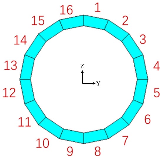
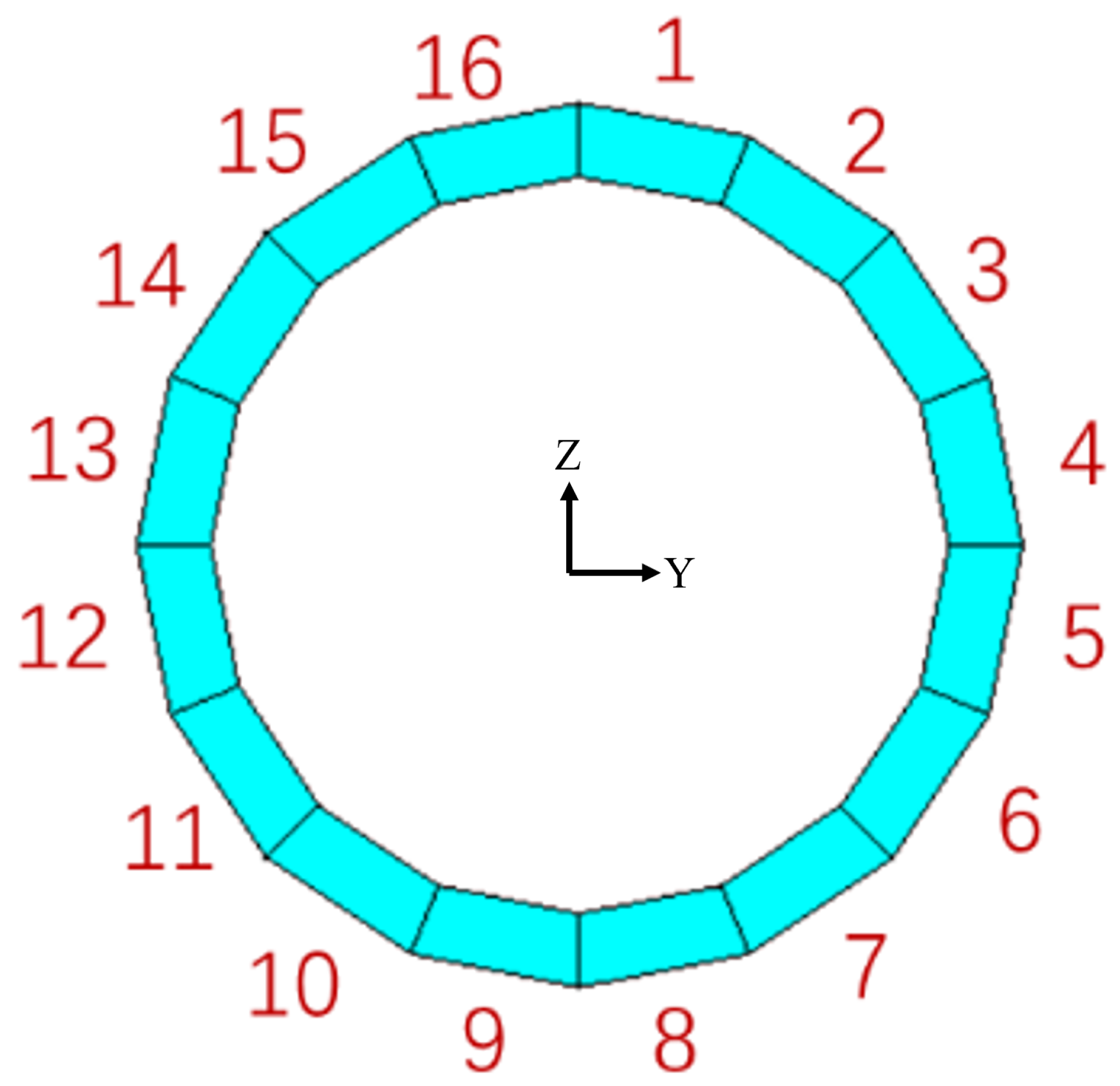
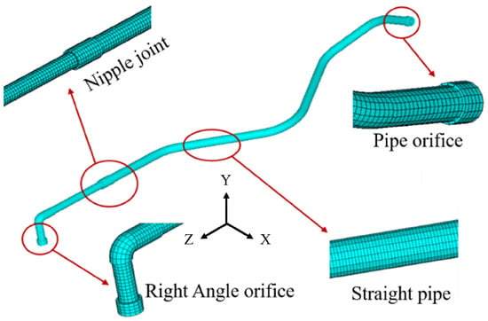
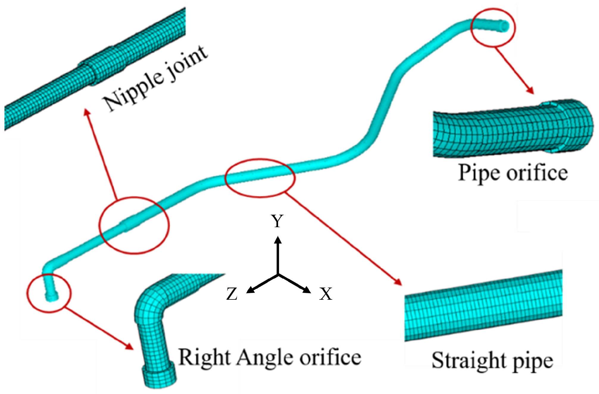
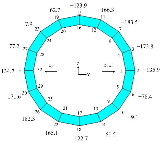
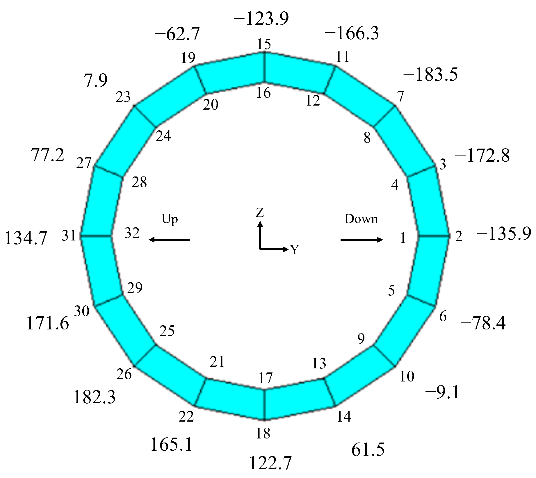
Considering both computational accuracy and speed in reconstruction, appropriate element size and quantity must be selected. In this study, pipe element PIPE289 and elbow element ELBOW290 are used to establish a simplified model of the aero-engine pipeline, with a mesh size of 5 mm and a total of 377 elements. According to the actual pipeline cross-section dimensions, the cross-section of the pipeline model element is divided into 16 parts, as shown in Figure 3, to obtain response data at different positions on the pipeline surface. Constraints imposed on the pipeline at clamps, supports and nozzles are simulated using the spring–damper element COMBIN14; the damping coefficient of COMBIN14 is set to 0.005 to represent the weak inherent damping of metal elastic supports, which is a typical empirical value for stainless steel pipeline brackets in engineering simulations. The pipeline structure is formed by connecting multiple straight pipes and elbows, with an outer diameter of 30 mm, inner diameter of 25 mm, and wall thickness of 2.5 mm. The material is 304 stainless steel. Based on the actual pipeline structure, the APDL simplified model of the pipeline shown in Figure 4 is established using parametric design language, which has been widely adopted in aerospace structural simulation for its high efficiency and flexibility [27,28].

Figure 3. Cross-section of pipe element.

Figure 4. Simplified model of pipeline.

3.2. Static Numerical Simulation and Experimental Verification of Pipeline Model

Establishing an APDL-based simplified model consistent with the actual structure is critical for subsequent load and constraint parameter reconstruction using intelligent algorithms. Therefore, static simulation analysis is carried out on the developed simplified model and compared with experimental data to verify model reliability.

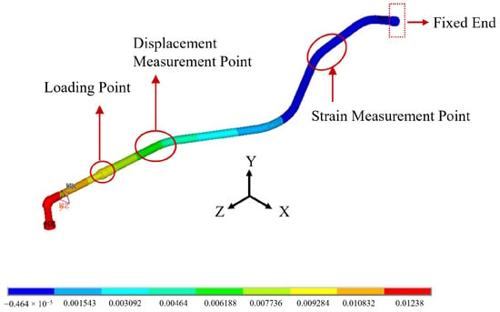
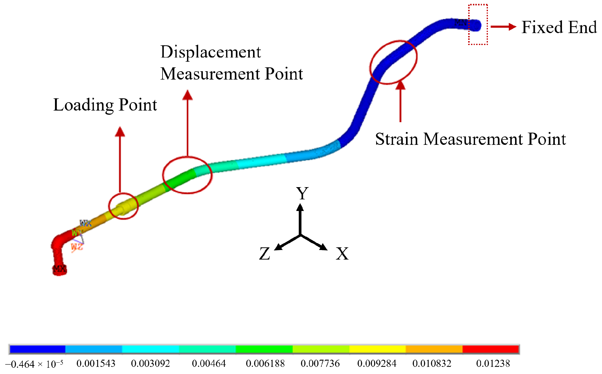
Fixed constraints are applied to the right nozzle of the above-mentioned simplified pipeline model, and static loads ranging from 5 kg to 23.6 kg are applied at the other side near the hoop clamp. The specific loading schematic is shown in Figure 5. The measurement points indicated in the figure are selected as displacement and strain monitoring points for comparison with experimental data.

Figure 5. Contour plot of static-load simulation for pipeline.

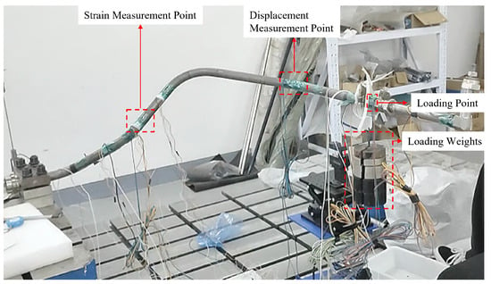
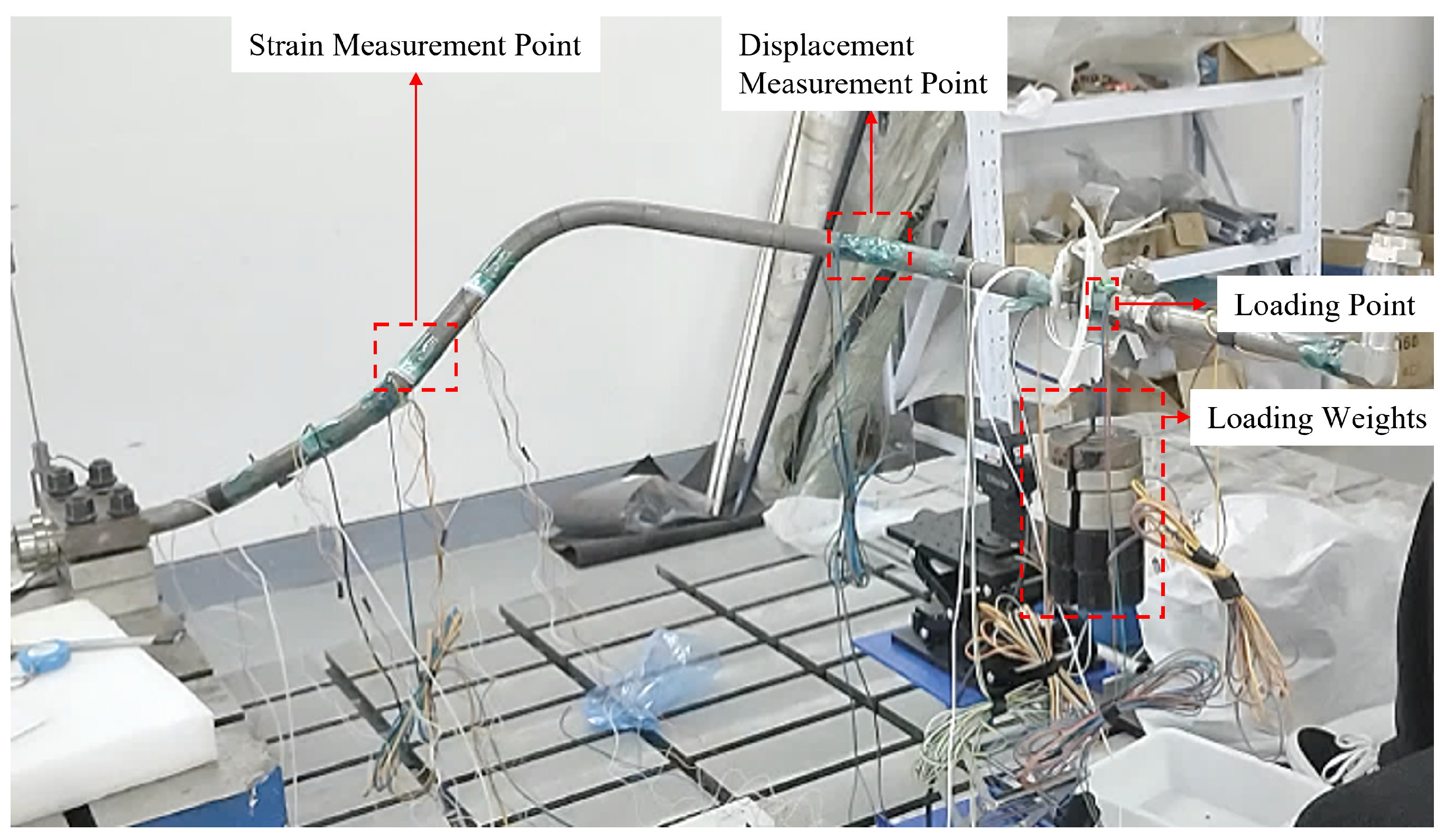
An experimental system as shown in Figure 6 is built, which consists of a measurement system and a loading system. The measurement system is composed of a dynamic strain indicator, strain gauges and supporting devices, while the loading system adopts loading blocks. The loading position as well as displacement and strain measurement points are consistent with those in the numerical simulation. The displacement and strain values at measurement points of the pipeline under static loads from 5 kg to 23.6 kg are measured. The comparison between simulation and experimental results is listed in Table 1.

Figure 6. Schematic diagram of static-load experiment for pipeline.

Table 1. Comparison between simulated and experimental displacement values at measurement points.

	5 kg	17.76 kg	19.76 kg	21.76 kg	23.6 kg
Experimental value (mm)	7.348	26.409	29.427	32.392	35.369
Simulation value (mm)	6.476	23.005	25.595	28.186	30.569
Error/%	11.87	12.89	13.02	12.98	13.57
Average error/%	12.87

As shown in Table 1, under static loads ranging from 5 kg to 23.6 kg, the maximum error between simulated and experimental displacement values at measurement points is 13.57%, the minimum error is 11.87%, and the average error is 12.87%, indicating relatively stable error performance.

Taking the 5 kg static-load condition as an example, numerical simulation results show the strain distribution on the pipeline cross-section at the strain measurement points in Figure 7. The strain values at the upper and lower surfaces of the cross-section are close in magnitude but opposite in sign, as listed in Table 2. Comparing the simulated cross-section strain distribution with experimental data reveals small discrepancies, with a maximum error of 8.81% and a minimum error of 1.42%. This indicates that the static-analysis results of the simplified pipeline model agree well with the actual structural performance of the pipeline.

Figure 7. Strain distribution on pipeline cross-section at strain measurement point.

Table 2. Comparison of simulated and experimental strain data at measurement points.

	Upper Surface Strain of Measurement Point	Lower Surface Strain of Measurement Point
Experimental value ($\mathsf{\mu }\epsilon$)	134.70	−135.90
Simulation value ($\mathsf{\mu }\epsilon$)	132.79	−162.87
Error/%	1.42	8.81

4. Parameter Reconstruction Based on Numerical Simulation Analysis

To verify the feasibility and effectiveness of the proposed intelligent algorithms in reconstructing load and constraint parameters of aero-engine pipeline structures, numerical simulation analysis is conducted on the pipeline. The stiffness parameters of single- and multiple-constraint springs are reconstructed using displacement responses at local measurement points on the pipeline, and the harmonic excitation loads acting on the pipeline are reconstructed using strain responses at local measurement points.

4.1. Parameter Reconstruction Based on Particle Swarm Optimization

According to the vibration load information and constraint conditions of the pipeline under aero-engine operating conditions, the structural responses under different types of excitations are obtained based on the pipeline vibration characteristics. Relying on the APDL platform and MATLAB software, reconstruction programs for pipeline loads and spring constraint stiffness are developed, and the computational data are exchanged between MATLAB and ANSYS [29,30].

First, ANSYS software is used to realize the functions of parametric modeling, loading, solving, and outputting response parameters of the pipeline. Then, the particle swarm iterative optimization algorithm is developed in MATLAB. The characteristic parameters output from ANSYS are imported into MATLAB to calculate the particle fitness function. Through continuous iteration, the input spring stiffness or excitation load amplitude corresponding to the minimum fitness is finally determined.

4.1.1. Reconstruction of Pipeline Constraint Parameters

(1) Reconstruction of Single-Spring Constraint Stiffness Parameter

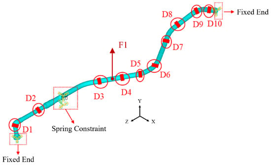
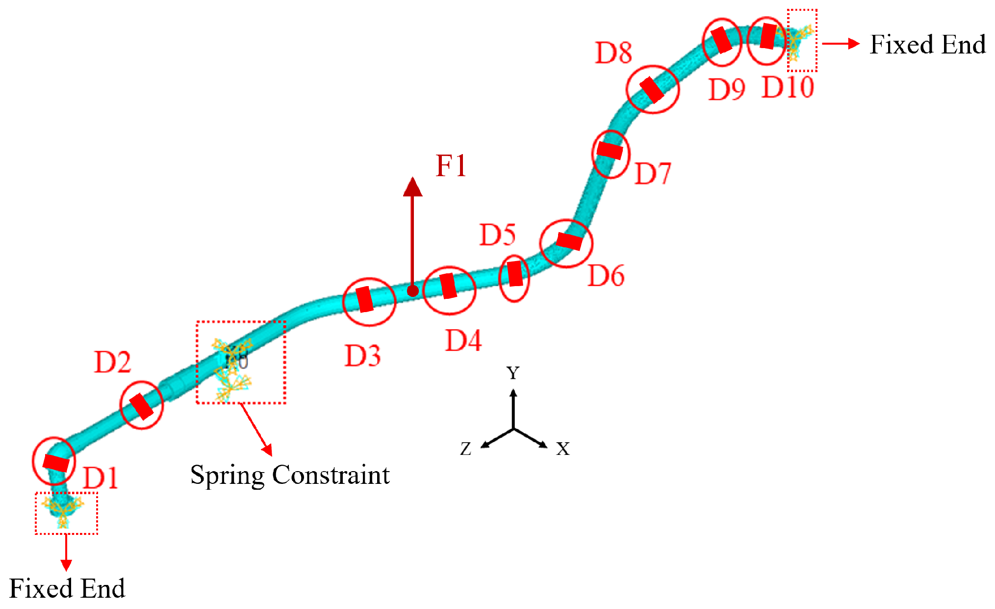
In the spring stiffness parameter reconstruction, a harmonic excitation of 30 Hz and 100 N is applied to the pipeline with both ends fixed. The constraint of the hoop clamp on the pipeline is simulated by the COMBIN14 spring element at the left clamp position. The harmonic excitation F is applied at the middle of the pipeline along the Y-axis, and 10 displacement measurement points D1–D10 are selected, as shown in Figure 8. The Y-direction displacements of the measurement points are chosen as the response parameters. The initial spring stiffness values (i.e., the initial particle velocities) are reasonably set in the particle swarm reconstruction algorithm. The co-simulation is carried out using ANSYS and MATLAB, and the constraint parameters are iteratively reconstructed with Equation (5) as the objective function. The results are presented in Table 3 and Table 4.

Figure 8. Schematic diagram of one-spring constraints and displacement measurement points.

Table 3. Reconstruction of single-spring constraint (without noise).

Applied Value/N·m/rad	Reconstructed Value/N·m/rad	Error/%	Average Error/%
1.00 × 104	1.011 × 104	1.10	0.73
1.00 × 105	9.938 × 104	0.62
1.00 × 106	9.952 × 105	0.48

Table 4. Reconstruction of single-spring constraint (with 5% noise).

Applied Value/N·m/rad	Reconstructed Value/N·m/rad	Error/%	Average Error/%
1.00 × 104	9.575 × 103	4.25	4.53
1.00 × 105	1.036 × 105	3.60
1.00 × 106	9.427 × 105	5.73

It can be seen that when reconstructing the pipeline spring constraints using displacement parameters based on the improved particle swarm optimization, the reconstruction accuracy is high without noise interference. For the inversion calculation of spring constraint stiffness values of 1.00 × 10⁴, 1.00 × 10⁵, and 1.00 × 10⁶, the maximum error is only 1.10%, and the average error is 0.73%. After introducing 5% random noise into the displacement parameters of the measurement points, the reconstruction accuracy decreases slightly, with a maximum error of 5.73% and an average error of 4.53%. Although the reconstruction accuracy is reduced after noise introduction, the reconstruction of spring stiffness still maintains high accuracy.

(2) Reconstruction of Two-Spring Constraint Stiffness Parameters

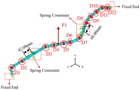
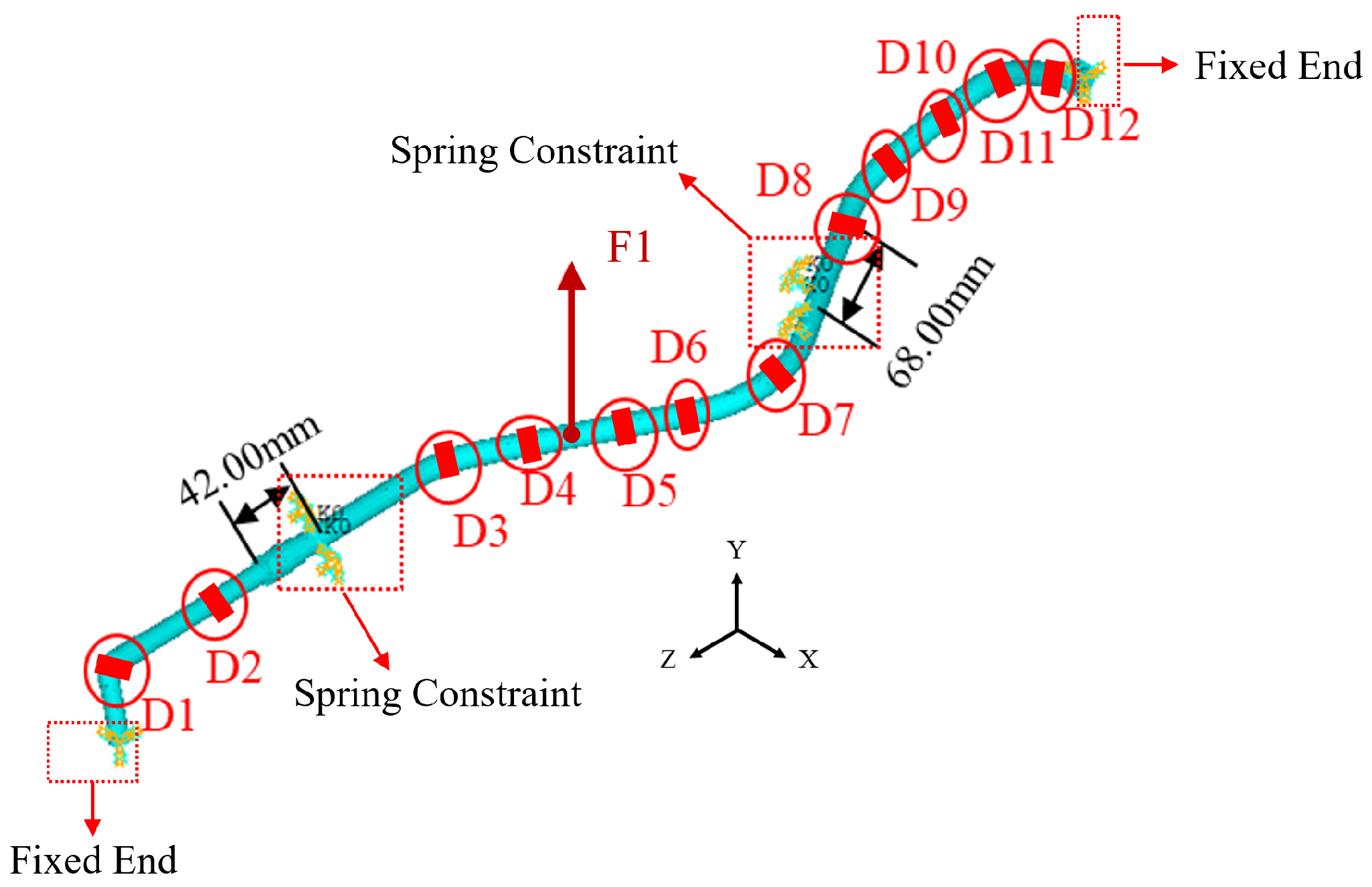
In the reconstruction of two-spring stiffness parameters, the constraint mode, excitation loading position and direction remain unchanged. COMBIN14 spring elements are used at the left and right clamp positions to simulate the constraints of the clamps on the entire pipeline, as shown in Figure 9, and the spring stiffness coefficients at the two clamps are set to be identical. The Y-direction displacements of 12 measurement points (D1–D12) shown in the figure are selected as response parameters to reconstruct two springs with the same stiffness coefficient. The results are presented in Table 5 and Table 6.

Figure 9. Schematic diagram of two-spring constraints and displacement measurement points.

Table 5. Reconstruction of two-spring constraints (without noise).

Applied Value/N·m/rad	Reconstructed Value/N·m/rad	Error/%	Average Error/%
1.00 × 104	9.883 × 104	1.17	1.06
1.00 × 105	1.009 × 105	0.90
1.00 × 106	1.011 × 106	1.10

Table 6. Reconstruction of two-spring constraints (with 5% noise).

Applied Value/N·m/rad	Reconstructed Value/N·m/rad	Error/%	Average Error/%
1.00 × 104	9.631 × 103	3.69	4.27
1.00 × 105	1.0437 × 105	4.37
1.00 × 106	9.526 × 105	4.74

The improved particle swarm optimization algorithm is adopted to reconstruct two-spring constraints with identical stiffness but different positions based on displacement parameters. When the spring constraint stiffness values are 1.00 × 10⁴, 1.00 × 10⁵ and 1.00 × 10⁶, the two-spring constraint parameters can be reconstructed accurately without noise interference, with a maximum error of 1.17% and an average error of 1.06%. After introducing 5% random noise into the displacement data of measurement points, the reconstruction errors increase compared with the noise-free condition, with a maximum error of 4.74% and an average error of 4.27%. The errors remain below 5%, which indicates that the improved particle swarm optimization algorithm can accurately reconstruct constraint information for two-spring constraints acting at different positions.

In the reconstruction of spring stiffness parameters using the improved particle swarm optimization algorithm, the upper bound of spring stiffness should be reasonably set to enable the algorithm to find the optimal solution more rapidly during iteration and improve the accuracy of inversion results. Generally, the upper bound of spring stiffness can be 10 to 100 times the true value, and the initial velocity for iterative optimization is set within the range of 10–20%. Since no lower bound of spring stiffness is specified, the search space of particles in the particle swarm is expanded, which better reflects the global optimization capability of the particle swarm optimization algorithm.

4.1.2. Reconstruction of Pipeline Load Parameters

(1) Amplitude Reconstruction of Single Harmonic Excitation

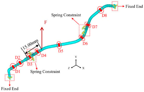
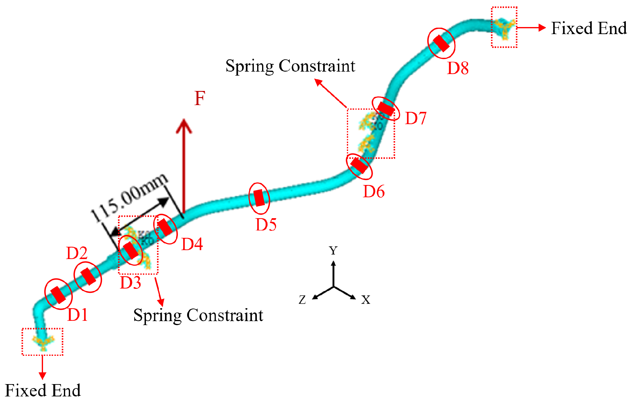
Numerous studies have shown that strain response parameters are more sensitive than displacement response parameters for load reconstruction based on particle swarm intelligence algorithms [29]. According to the actual stress conditions, the amplitude of the sinusoidal excitation along the Y-axis applied near the left pipeline clamp is set as the variable to be inverted. The specific loading conditions are listed in Table 7. The Y-direction strain values of eight measurement points D1 D8 on the pipeline are taken as characteristic parameters, and Equation (5) is used as the objective function to invert the excitation amplitude. The schematic diagram of excitation loading is shown in Figure 10.

Table 7. Loading condition table.

Load Type	Force	Frequency
Harmonic	50 N	30 Hz
	100 N
	200 N
	500 N

Figure 10. Schematic diagram of single harmonic excitation loading and measurement point positions.

It can be seen from Table 8 and Table 9 that the particle swarm optimization algorithm can accurately reconstruct the single harmonic excitation applied to the pipeline. Under noise-free conditions, the maximum reconstruction error for excitations of 50 N, 100 N, 200 N and 500 N is 0.54%, with an average error of 0.37%. When 5% noise is added to the strain response parameters, the reconstruction error rises to 3.24%, and the average error increases to 2.66%.

Table 8. Reconstruction results of single harmonic excitation on pipeline (without noise).

Applied Value/N	Reconstructed Value/N	Error/%	Average Error/%
50.00	49.95	0.10	0.37
100.00	100.54	0.54
200.00	199.02	0.49
500.00	501.73	0.35

Table 9. Reconstruction results of single harmonic excitation on pipeline (with 5% noise).

Applied Value/N	Reconstructed Value/N	Error/%	Average Error/%
50.00	48.38	3.24	2.66
100.00	102.57	2.57
200.00	194.36	2.82
500.00	489.98	2.00

(2) Amplitude Reconstruction of Two Harmonic Excitations

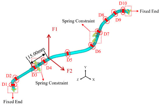
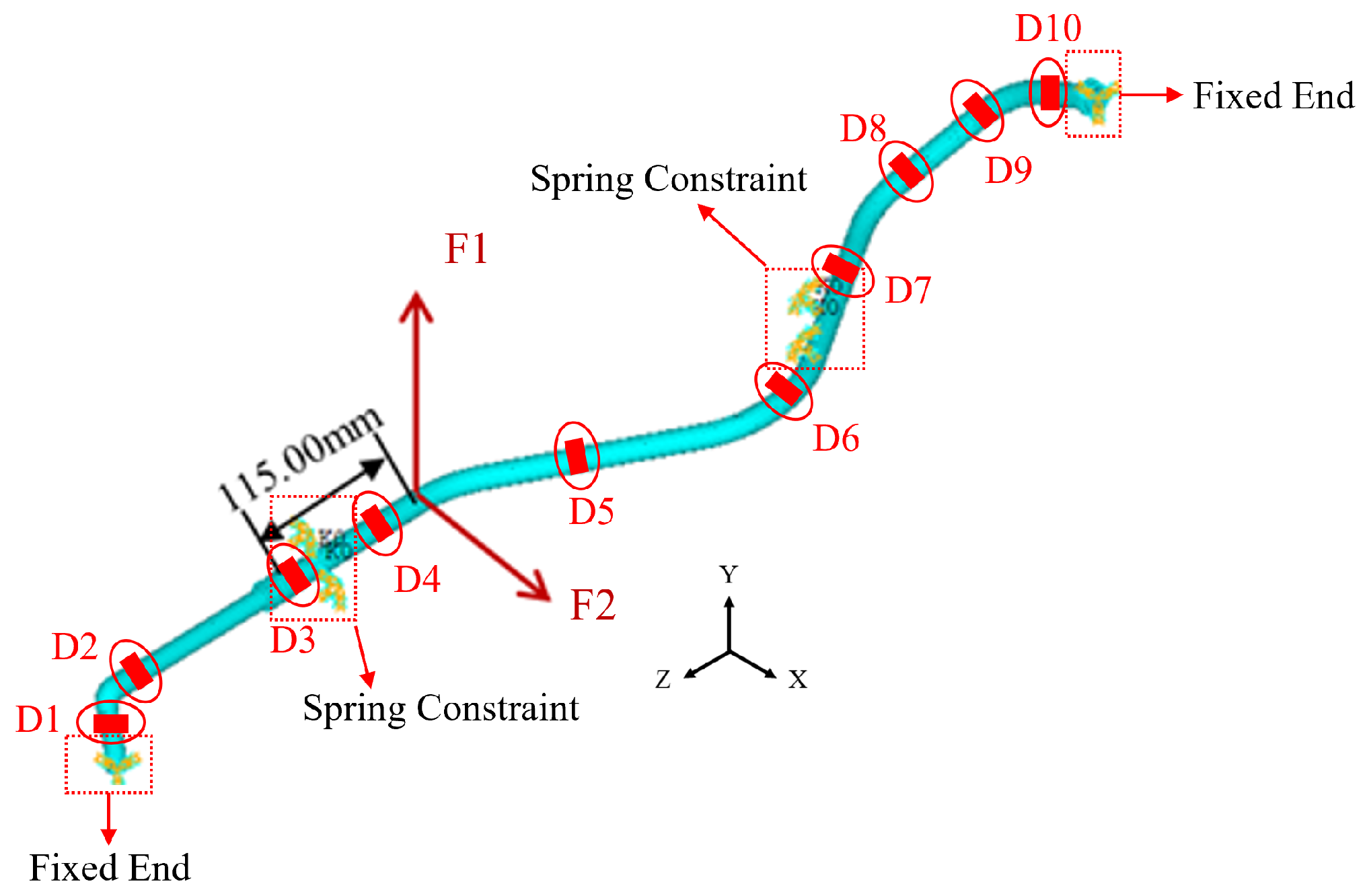
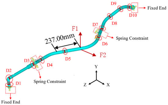
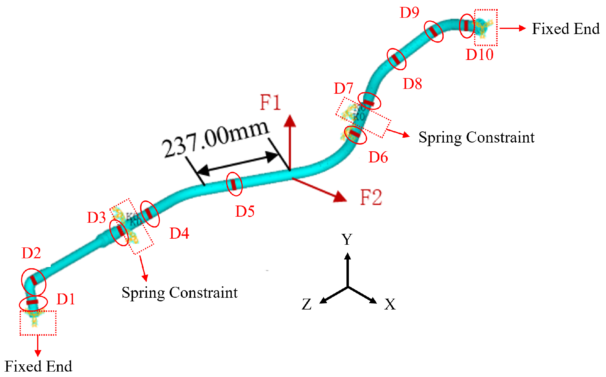
When an aero-engine is in operation, the internal pipeline bears complex loads. Reconstructing only the amplitude of single-direction harmonic excitation cannot accurately simulate the complex excitations acting on the pipeline in service. Therefore, it is necessary to reconstruct harmonic excitations acting simultaneously in multiple directions. Arbitrary forces in a plane or space can be synthesized by the principle of force composition and decomposition. In this study, the amplitudes of sinusoidal excitations applied near the left pipeline clamp are set as inversion variables, with excitation directions along both the X-axis and Y-axis. The excitation loading position is consistent with that of the single harmonic excitation, as shown in Figure 11, and the loading conditions are listed in Table 10. The X- and Y-direction strain values of 10 measurement points D1–D10 on the pipeline are taken as characteristic parameters, with 5% noise added to these parameters. Two harmonic excitations with the same frequency but different amplitudes are reconstructed simultaneously, and the results are presented in Table 11. It can be seen from Table 11 that the reconstruction accuracy decreases and the error increases with the increase in the number of loads when reconstructing two-direction harmonic excitations at the same position on the pipeline. Under the working condition of 100–1000 N, the maximum load reconstruction error is 15.83% and the average error is 6.65%.

Figure 11. Schematic diagram of two-harmonic-excitation loading and measurement point positions.

Table 10. Loading condition table.

Motivation Direction	Load Size			Frequency
X (F1)	−1000 N	−500 N	100 N	30 Hz
Y (F2)	−800 N	500 N	1000 N

Table 11. Simultaneous reconstruction of two harmonic excitations on pipeline (with 5% noise).

	Applied Value/N	Reconstructed Value/N	Error/%	Average Error/%
F1	−1000	−957.33	4.63	6.65
	−500	−475.75	4.85
	100	84.17	15.83
F2	−800	−758.08	5.24
	500	530.85	6.17
	1000	1031.76	3.18

(3) Amplitude Reconstruction of Four Harmonic Excitations

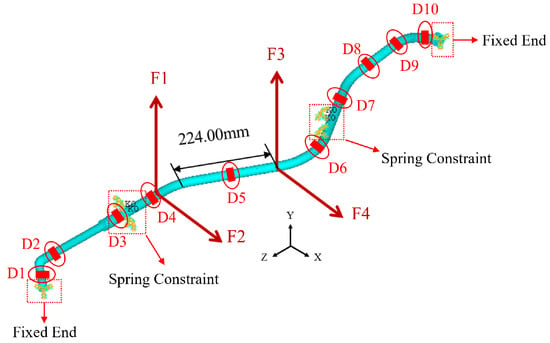
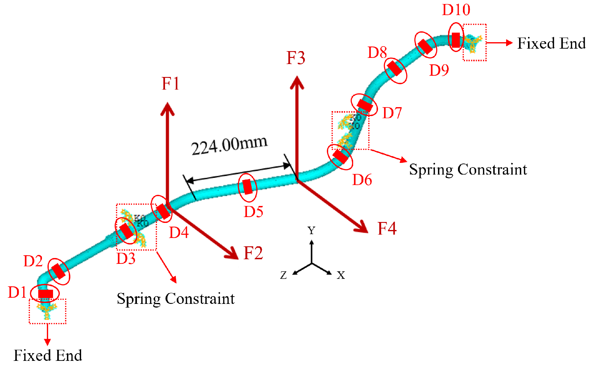
To more accurately simulate the real excitations acting on aero-engine pipelines, four harmonic excitations of 30 Hz are applied simultaneously to the pipeline structure, and 5% noise is added to the characteristic parameters. The excitation loading positions are shown in Figure 12. The particle swarm optimization algorithm is used to reconstruct the amplitudes of the four loads on the pipeline, and the results are shown in Table 12 below. With the increase in the number of loads with different amplitudes, the reconstruction errors of the particle swarm optimization algorithm increase significantly. The maximum error exceeds 20%, reaching 24.9%, and the average error exceeds 10%, reaching 11.12%. This indicates that the applicability of the improved particle swarm optimization algorithm in structural load reconstruction still needs further optimization.

Figure 12. Schematic diagram of four-harmonic-excitation loading and measurement point positions.

Table 12. Simultaneous reconstruction of four harmonic excitations on pipeline (with 5% noise).

	Applied Value/N	Reconstructed Value/N	Error/%	Average Error/%
F1	100	75.11	24.90	11.12
F2	200	217.45	8.73
F3	500	471.45	5.71
F4	1000	1051.27	5.13

4.2. Harmonic Excitation Load Parameter Reconstruction Based on Conjugate Gradient Method

In Section 4.1 above, the improved particle swarm optimization algorithm was adopted to reconstruct stiffness parameters of single-spring constraints and two-spring constraints. For single-spring constraint stiffness reconstruction, the average error was 0.73% without noise and 4.53% with 5% random noise introduced. For two-spring constraint stiffness reconstruction, the average error was 1.06% without noise and 4.27% with 5% random noise. The errors under both conditions were lower than 5%, achieving relatively high reconstruction accuracy. Therefore, the conjugate gradient method is not used for reconstruction under these two conditions, but only for harmonic excitations. Due to the complex load distribution, it is necessary to identify and reconstruct multiple-direction and multiple-harmonic loads acting simultaneously on the pipeline.

(1) Amplitude Reconstruction of Single Harmonic Excitation

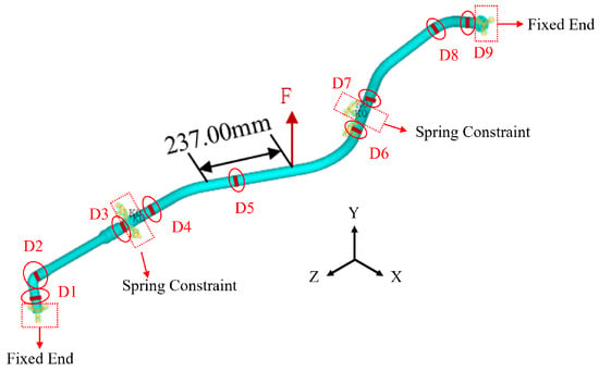
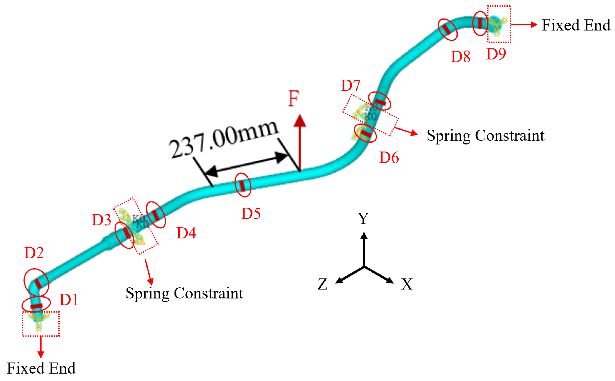
Single sinusoidal excitation amplitude reconstruction is carried out for the pipeline structure shown in Figure 13. The pipeline is fixed at both ends. Spring elements in two radial directions are used at the two hoop clamp positions in the middle of the pipeline to simulate clamp constraints, with a spring stiffness coefficient of $1.00\times {10}^4$ N·m/rad. Sinusoidal excitations with a frequency of 30 Hz and amplitudes of 100 N, 500 N and 1000 N are applied radially to the pipeline, with the amplitudes taken as inversion variables. Axial strain data from nine measurement points on the pipeline are used as characteristic parameters for reconstruction.

Figure 13. Schematic diagram of single-harmonic-excitation loading and measurement point positions.

Table 13 and Table 14 present the reconstruction results of the three groups of sinusoidal load amplitudes. It can be seen that the single-direction harmonic excitation amplitude applied in the middle of the pipeline can be accurately reconstructed using the nine axial strain values obtained from simulation results, with a maximum error of only 0.25% and an average error of 0.13%. After adding 5% noise to the simulation results, the maximum reconstruction error increases to 0.76% and the average error rises to 0.62%. Thus, the conjugate gradient method exhibits good noise immunity in single-load reconstruction.

Table 13. Reconstruction of single-spring constraint (without noise).

Applied Value/N	Reconstructed Value/N	Error/%	Average Error/%
100	99.86	0.14	0.13
500	501.27	0.25
1000	999.98	0.00

Table 14. Reconstruction results of single harmonic excitation on pipeline (with 5% noise).

Applied Value/N	Reconstructed Value/N	Error/%	Average Error/%
100	100.75	0.75	0.62
500	496.20	0.76
1000	996.42	0.36

(2) Amplitude Reconstruction of Two Harmonic Excitations

Given the complex loads acting on the pipeline structure under engine service conditions, it is necessary to reconstruct excitation amplitudes for cases where the pipeline is simultaneously subjected to two-directional or even more harmonic excitations to verify algorithm effectiveness. The constraint conditions remain unchanged. Two harmonic excitations with a frequency of 30 Hz are applied simultaneously in two directions at the positions shown in Figure 14. Then, 5% random noise is added to strain values at 10 locations on the pipeline, which are taken as characteristic parameters for reconstructing excitation amplitudes. The amplitudes of excitations applied in the middle of the pipeline are reconstructed, and the results are shown in Table 15. The results indicate that, with 5% noise, the maximum error of excitation amplitude reconstruction using 10 axial strain values from harmonic response simulation is 6.63%, and the average error is 3.28%. This demonstrates that the conjugate gradient method can accurately reconstruct the amplitudes of two-directional harmonic excitations applied simultaneously in the middle of the pipeline.

Figure 14. Schematic diagram of two-harmonic-excitation loading and measurement point positions.

Table 15. Simultaneous reconstruction of two harmonic excitations on pipeline (with 5% noise).

	Applied Value/N	Reconstructed Value/N	Error/%	Average Error/%
F1	−1000	−986.15	1.39	3.28
	−800	−783.22	2.13
	100	93.37	6.63
F2	−500	−480.11	3.98
	−450	−438.10	2.73
	1000	1028.64	2.86

(3) Amplitude Reconstruction of Four Harmonic Excitations

To verify more complex loading conditions, the case where the pipeline is simultaneously subjected to four harmonic excitations is simulated. The specific loading conditions are consistent with those used for four-excitation amplitude reconstruction via the improved particle swarm optimization algorithm, and 5% noise is added to the characteristic parameters. The reconstruction results of the four loads are presented in Table 16. The four applied excitation amplitudes can be reconstructed accurately, with a maximum error of 5.16% and an average error of 4.48%. Since the conjugate gradient method adopts conjugate search directions, it can effectively avoid the local convergence problem that commonly occurs in the particle swarm optimization algorithm.

Table 16. Simultaneous reconstruction of four harmonic excitations on pipeline (with 5% noise).

	Applied Value/N	Reconstructed Value/N	Error/%	Average Error/%
F1	−1000	−1051.6	5.16	4.48
F2	−500	−478.60	4.28
F3	1000	1047.51	4.75
F4	500	518.67	3.73

4.3. Analysis of Algorithm Reconstruction Errors

In this section, the IPSO algorithm is first employed for load amplitude reconstruction based on numerical simulation data. The proposed IPSO performs well in the inversion of single-spring and dual-spring constraint stiffness, demonstrating favorable stability and identification precision. For the single harmonic excitation case, the algorithm maintains high reconstruction accuracy, with a maximum error of 3.24% and an average error of 2.66%. However, obvious accuracy degradation occurs when reconstructing multiple harmonic excitation amplitudes simultaneously. For dual harmonic excitations acting on the same pipeline position, reconstruction errors increase with the quantity of unknown loads, where the maximum error reaches 15.83% and the average error is 6.65%. When four independent load amplitudes are inverted together, the maximum reconstruction error rises to 24.9% and the average error reaches 11.12%. The core root of this phenomenon lies in the inherent drawbacks of population random search under high-dimensional coupled inverse problems. Multi-load identification introduces a large number of strongly coupled unknown variables, generating a complex multi-modal objective function full of local optima. Although the IPSO adopts coordinated linear adjustment of inertia weight and learning factors to balance global and local search, this improvement cannot fundamentally eliminate premature convergence. As the load dimension expands, particles lose global exploration capability and converge to local optima prematurely, leading to unacceptable reconstruction errors for multi-load cases.

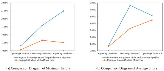
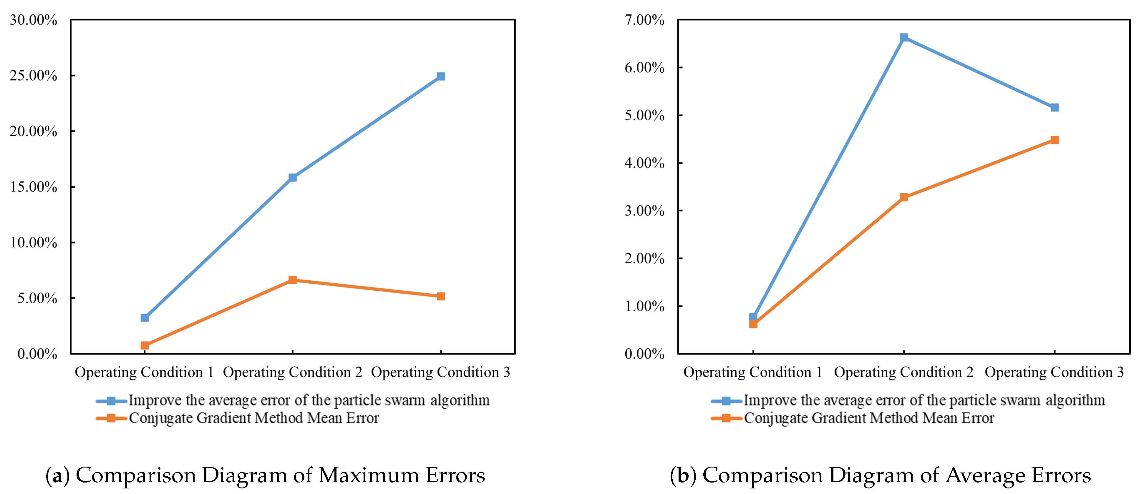
To address the low accuracy of the IPSO algorithm in multi-load amplitude reconstruction, a load amplitude reconstruction algorithm based on the CGM is proposed in this paper. When reconstructing static-load amplitudes with this algorithm, the maximum error is 3.94%, demonstrating high accuracy for static-load reconstruction. Compared with the IPSO algorithm, the CGM achieves substantially lower errors in single harmonic excitation amplitude reconstruction, with a maximum error of 0.76% and an average error of 0.62%, reducing the average error by 76.69%. For multi-harmonic excitation amplitude reconstruction, the maximum error for two-directional harmonic excitations at the same position is 6.63%, with an average error of 3.28%, which is a 50.68% reduction in average error relative to the IPSO. For four-load amplitude reconstruction, the maximum error is 5.16% and the average error is 4.48%, representing a 59.71% reduction in average error. The proposed conjugate-gradient-based load amplitude reconstruction algorithm greatly improves reconstruction accuracy and applicability under complex loading conditions compared with the IPSO algorithm. The comparison of reconstruction errors between the IPSO algorithm and the CGM is shown in Table 17, and the error comparison diagram is presented in Figure 15.

Table 17. Comparison table of reconstruction errors between improved PSO algorithm and conjugate gradient method.

Working Condition	IPSO		CGM
	Maximum Error (%)	Average Error (%)	Maximum Error (%)	Average Error (%)
Amplitude Reconstruction of Single Harmonic Excitation	3.24	2.26	0.76	0.62
Amplitude Reconstruction of Two Harmonic Excitations	15.83	6.65	6.63	3.28
Amplitude Reconstruction of Four Harmonic Excitations	24.9	11.12	5.16	4.48

Figure 15. Comparison diagram of reconstruction errors between improved PSO algorithm and conjugate gradient method.

5. Experimental Verification

5.1. Construction of Experimental System

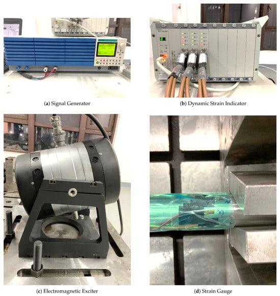
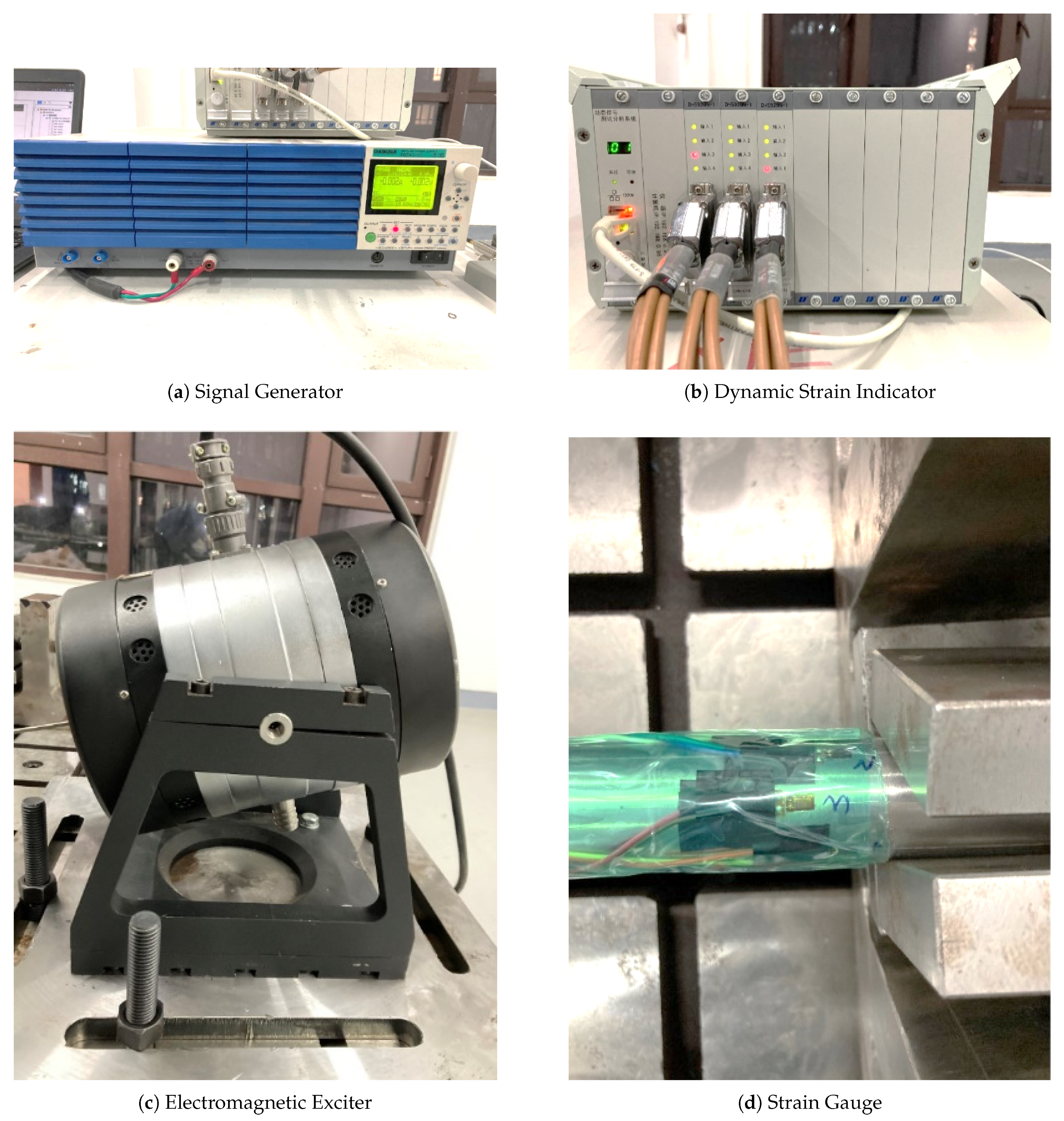
The conjugate gradient method achieves high accuracy in load reconstruction of aero-engine pipelines. Even with 5% random errors in strain data, it can accurately reconstruct static loads and harmonic excitation amplitudes acting on the pipeline. To verify the engineering effectiveness of the algorithm, an experimental system is established to collect response signals of the tested pipeline. The testing equipment and devices of the experimental system consist of an excitation system, a measurement system, a data acquisition and processing system, and supporting devices, mainly including a signal generator, an electromagnetic exciter, a force sensor, a charge amplifier, strain gauges, a 12-channel dynamic strain indicator, a supporting steel frame, and a supporting base. Strain gauges are adopted for strain data acquisition of the pipeline system. They are pasted as close as possible to regions prone to maximum stress, such as welds, branch pipe joints and elbow sections, while avoiding stress concentration areas. A sufficient number of strain gauges are reasonably arranged according to the requirements of parameter reconstruction. The main instruments used in the vibration experiment are shown in Figure 16.

Figure 16. Main experimental equipment.

5.2. Experiment on Harmonic Excitation Parameter Reconstruction

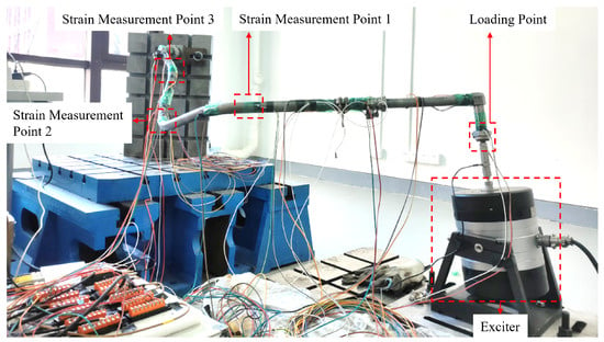
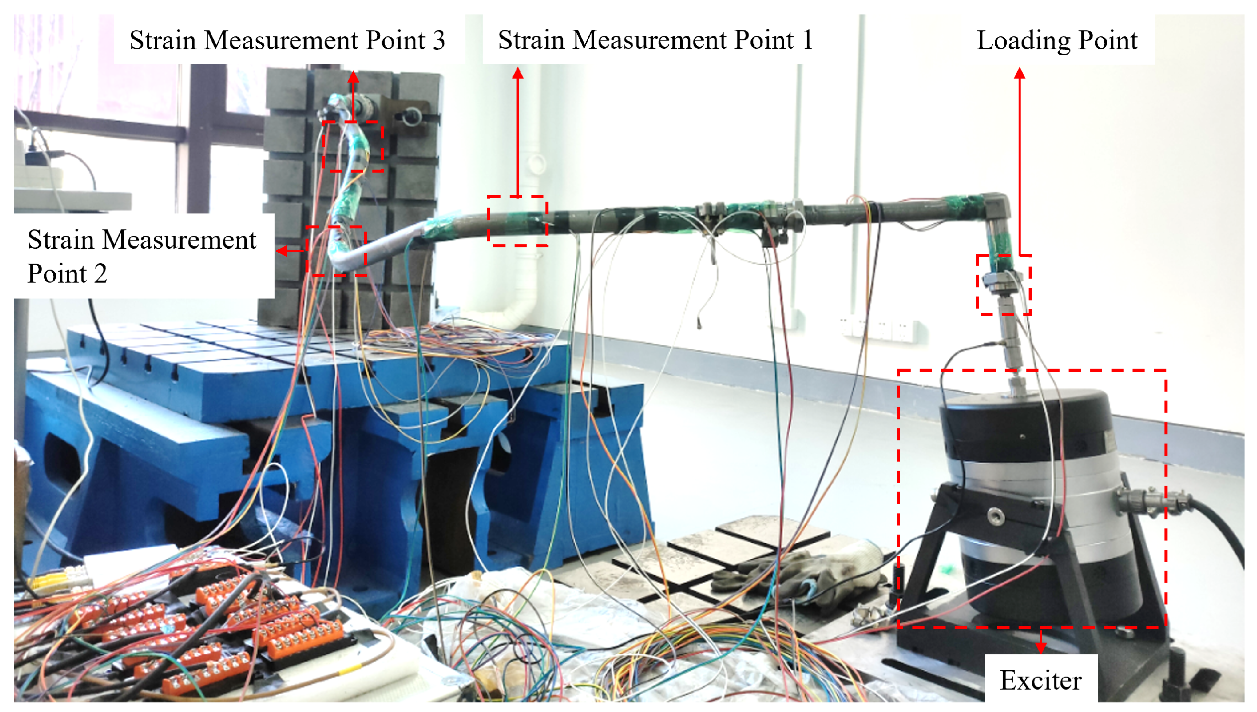
Before conducting the harmonic excitation load reconstruction experiment, the vibration exciter, dynamic force sensor and right straight pipe section are rigidly connected, and the mounting angle of the exciter is adjusted to a suitable position. The harmonic excitation force produced by the exciter is delivered to the pipeline port through a rigid push rod. A dynamic force sensor is arranged between the rigid rod and pipeline port to capture and record the real-time amplitude fluctuation of the harmonic excitation force during loading.

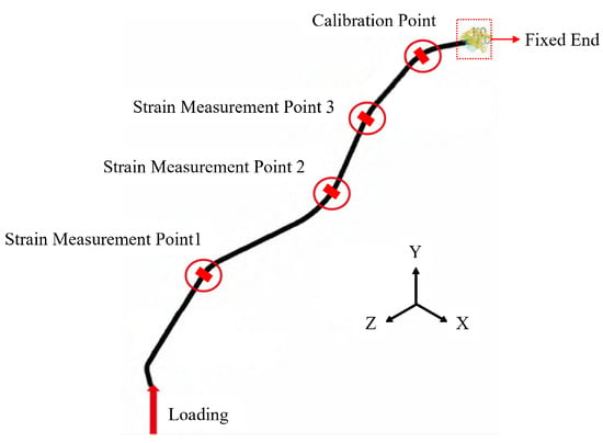
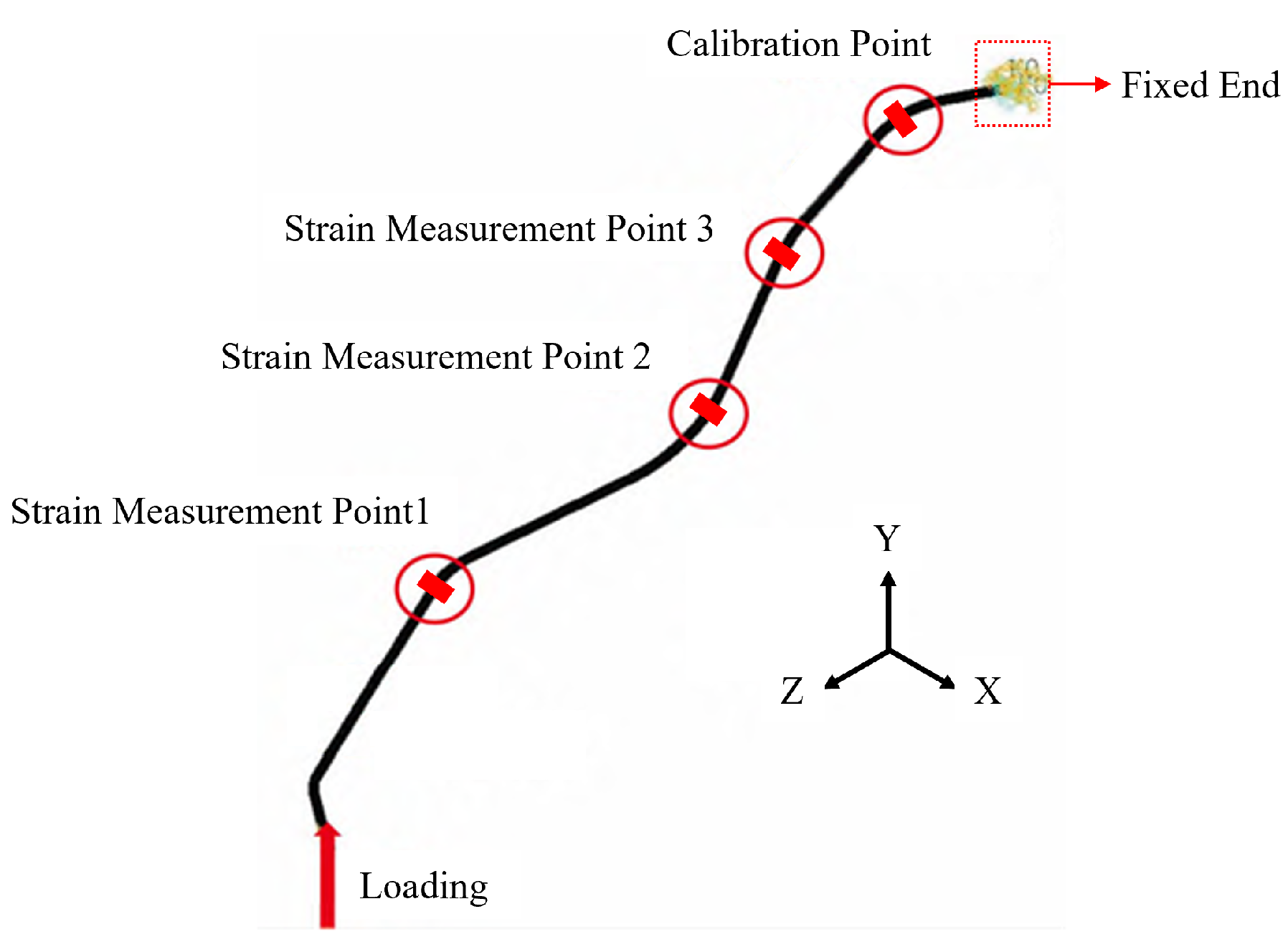
A total of six metal strain gauges are deployed at three critical stress measuring points (one gauge on the upper wall and one on the lower wall at each point) to collect dynamic strain signals. The sampling frequency of the strain acquisition system is set to 2000 Hz, satisfying the Nyquist sampling theorem for the maximum 80 Hz excitation frequency. A full-bridge circuit with temperature compensation chips and a built-in 100 Hz low-pass filter is adopted for signal conditioning to suppress environmental noise. All strain gauges are wired to the dynamic strain testing system for real-time data recording. The schematic layout of harmonic excitation loading and measuring points is shown in Figure 17, and the hardware composition of the entire experimental measurement system is demonstrated in Figure 18.

Figure 17. Schematic diagram of harmonic excitation loading and measuring point positions of experimental pipeline.

Figure 18. Schematic of harmonic excitation loading test on pipeline.

Raw strain data collected by the acquisition system are prone to outliers induced by ambient noise, contact friction and signal drift. To eliminate invalid interference, data points that significantly diverge from the periodic strain trend are removed, and the filtered measurement data are presented in Table 18. For the test case with 80 Hz and 60.93 N harmonic excitation, upper and lower surface strain values from the three valid measuring points are contrasted with finite element predictions under identical operating conditions. The relative error between experimental and simulated strain ranges from 3.77% to 19.47%. This discrepancy originates from multiple sources, including idealized model simplifications, semi-rigid fixture boundaries, material parameter deviations and inherent measurement noise. After comprehensive evaluation of these coupled influencing factors, the processed strain data are considered reliable for load reconstruction. On the basis of the filtered strain measurements, the harmonic excitation amplitude acting on the pipeline is inversely reconstructed, with detailed results recorded in Table 19. The reconstructed excitation force is 52.52 N, producing a relative error of 14.24%. Although the reconstruction error is non-negligible, the achieved identification precision meets the acceptance standard for real engineering vibration testing environments.

Table 18. Strain data of pipeline under harmonic excitation.

Frequency	Load	Type	Strain 1/$\mathsf{\mu }\mathit{\epsilon }$		Strain 2/$\mathsf{\mu }\mathit{\epsilon }$	Strain 3/$\mathsf{\mu }\mathit{\epsilon }$
			Up	Down	Up	Up	Down
80 Hz	60.93 N	Experiment	65.20	67.35	26.95	31.13	19.70
		Simulation	62.84	62.38	29.92	26.40	24.46
		Error	3.77%	7.96%	9.95%	17.95%	19.47%

Table 19. Reconstructed load values of pipeline under harmonic excitation.

Frequency	Experimental Load	Reconstructed Load	Error
80 Hz	60.93 N	52.25 N	14.24%

6. Conclusions

This study develops a two-stage inverse reconstruction framework combining IPSO and the CGM to identify support spring stiffness and harmonic excitation loads of aero-engine pipelines. Relying on the data interaction interface between MATLAB and ANSYS, an inverse simulation platform is constructed, and a dual-algorithm collaborative parameter reconstruction method for pipeline constraints and dynamic loads is proposed.

Numerical tests reveal that the IPSO can accurately invert spring stiffness parameters utilizing structural displacement responses. With 5% random noise superimposed on displacement data, the maximum identification error of support stiffness is only 5.37%. However, the identification accuracy of IPSO declines sharply with the growth in unknown harmonic loads. Under 5% noise interference, the maximum reconstruction error increases to 15.83% for dual harmonic loads and climbs to 24.9% for four coupled excitations. The multi-variable strongly coupled objective function of multi-load inversion presents abundant local optimal solutions, which severely restricts the global search ability of IPSO and renders the algorithm ineffective for multi-load identification.

Given the inherent limitation of IPSO in multi-load inversion, this paper introduces the CGM for harmonic load reconstruction. Numerical simulations covering single, dual and quadruple harmonic excitation conditions are carried out. When 5% random noise is added to strain signals, the average amplitude reconstruction errors of all load cases are less than 5%. Physical experiments are only performed under a single harmonic excitation (60.93 N, 80 Hz) due to the lack of multi-channel synchronous excitation hardware in the laboratory. For experimental strain data containing 3.77–19.47% measurement deviation, the CGM restricts load reconstruction error within 15%, demonstrating strong anti-interference performance for pipeline dynamic load identification.

In summary, the IPSO is suitable for single-type spring constraint inversion while the CGM exhibits stable and robust performance for harmonic load reconstruction under different noise levels. Limited by the research objective targeting the practical installation state of the studied pipeline, all numerical simulations adopt fixed–fixed boundary conditions, and the identification performance under other constraint forms, such as simply supported and elastically supported boundaries, is not discussed in this paper. Subsequent work will establish a multi-channel synchronous vibration excitation system to complete experimental verification of multi-coupled harmonic loads, carry out extended research on diverse pipeline boundary constraints, further enrich the experimental basis of the proposed reconstruction method, and promote its application in actual aero-engine pipeline systems.

References

- Liang, X.; Wang, S.; Shen, W. Analysis of bubble flow in an inclined tube and modeling of flow prediction. Aerospace 2024, 11, 655. [Google Scholar] [CrossRef] [Scilit]
- Yan, Y.; Chai, M. Sealing failure and fretting fatigue behavior of fittings induced by pipeline vibration. Int. J. Fatigue 2020, 136, 105602. [Google Scholar] [CrossRef] [Scilit]
- Wang, Y.L.; Ma, W.J.; Liao, R.D.; He, K.; Li, X.F. Fatigue-resistant structural optimization and vibration testing of a spherical tube fitting in liquid rocket engines. Aerosp. Sci. Technol. 2026, 173, 111802. [Google Scholar] [CrossRef] [Scilit]
- Ge, C.Y.; Song, Z.B.; Zhou, C.H.; Guo, H.Q.; Zhu, D.M.; Wang, B. A novel accelerated fatigue test method of mission synthesis considering the segmented S-N curve. Int. J. Fatigue 2025, 193, 108789. [Google Scholar] [CrossRef] [Scilit]
- Pollock, L.; Abdelwahab, A.K.; Murray, J.; Wild, G. The Need for Aerospace Structural Health Monitoring: A review of aircraft fatigue accidents. Int. J. Progn. Health Manag. 2021, 12, 1–16. [Google Scholar] [CrossRef] [Scilit]
- Raghavendra, K.; Madan, M.; Venkatesh, V.; Sujata, M.; Bhaumik, S. Failure Analysis of a Welded AISI321 Steel Bleed Air Connector of an Aircraft Engine. J. Fail. Anal. Prev. 2022, 22, 1776–1786. [Google Scholar] [CrossRef] [Scilit]
- Hansen, M. On predicting and improving the condition of modal-model-based indirect force measurement algorithms. In Proceedings of the Proceedings, 8th International Modal Analysis Conference, Kissimmee, FL, USA, 29 January–1 February 1990; pp. 115–120. [Google Scholar]
- Reynders, E. System identification methods for (operational) modal analysis: Review and comparison. Arch. Comput. Methods Eng. 2012, 19, 51–124. [Google Scholar] [CrossRef] [Scilit]
- Miao, B.; Zhou, F.; Jiang, C.; Chen, X.; Yang, S. A comparative study of regularization method in structure load identification. Shock Vib. 2018, 2018, 9204865. [Google Scholar] [CrossRef] [Scilit]
- Chen, S.; Guo, A.; Wu, S.; Fei, Q. Dynamic load identification of satellite-rocket interface based on BP neural network. J. Vib. Shock 2023, 42, 279–286. [Google Scholar] [CrossRef]
- Liu, B.; Liu, Y.; Lian, Z.; Wu, Z.; He, L.; Yang, L. A Reconstruction Method for Weak Magnetic Pipeline Inspection Signals Based on Adaptive Multiscale Signal Reconstruction. IEEE Trans. Instrum. Meas. 2025, 74, 9517916. [Google Scholar] [CrossRef] [Scilit]
- Jiang, Z.; Wang, Y.; Yang, Y.; Zhou, J.; Shi, L. Research on Noise Reduction Method for Leakage Signal of Water Supply Pipeline. IEEE Access 2024, 12, 71406–71418. [Google Scholar] [CrossRef] [Scilit]
- Zhang, L.; Xie, J.; Xu, Q.; Koch, C.R.; Dubljevic, S. Physics-informed neural networks for state reconstruction of hydrogen energy transportation systems. Comput. Chem. Eng. 2025, 192, 108898. [Google Scholar] [CrossRef] [Scilit]
- Han, B.; Wang, C.; Zhang, X.; Zhao, Z.; Zhai, Z.; Liu, J.; Liu, N.; Chen, X. Pose Estimation and Neural Implicit Reconstruction Toward Noncooperative Spacecraft Without Offline Prior Information. IEEE Trans. Aerosp. Electron. Syst. 2024, 61, 2612–2630. [Google Scholar] [CrossRef] [Scilit]
- Gao, X.; Chen, H.E.; Li, Y.; Li, S.; Chen, H.; Wang, M.; Yang, S.; Tian, S.; Chen, Z. Reconstruction schemes of load and constraint for global vibration evaluation of pipeline structures. Int. J. Appl. Electromagn. Mech. 2023, 71, S589–S597. [Google Scholar] [CrossRef] [Scilit]
- Christensen, S.L.; Riis, N.A.; Pereyra, M.; Jørgensen, J.S. A Bayesian approach for CT reconstruction with defect detection for subsea pipelines. Inverse Probl. 2024, 40, 025003. [Google Scholar] [CrossRef] [Scilit]
- Jin, A.; Chen, C.; Yang, B.; Zou, Q.; Wang, Z.; Yan, Z.; Wu, S.; Zhou, J. Gpr-former: Detection and parametric reconstruction of hyperbolas in gpr b-scan images with transformers. IEEE Trans. Geosci. Remote Sens. 2024, 62, 4507113. [Google Scholar] [CrossRef] [Scilit]
- Wang, P.; Zhao, F.; Fu, X.; Liu, T.; Liu, L. Visualization of Clogging Detection in Mine Artesian Filling Pipes Based on ERT Technology. IEEE Sens. J. 2025, 25, 33840–33848. [Google Scholar] [CrossRef] [Scilit]
- Zhou, X.; Yin, W.; Yang, K. Adaptive acoustic leak location of long buried pipe via transient optimization statistical analysis. IEEE Trans. Instrum. Meas. 2024, 73, 3510110. [Google Scholar] [CrossRef] [Scilit]
- Xu, X.; Zhu, Y.; Tian, K.; Lin, T.; Li, Y. Study on an integral algorithm of load identification based on displacement response. Sensors 2021, 21, 6403. [Google Scholar] [CrossRef] [Scilit] [PubMed]
- Zhang, Z.J.; Pan, Y.Y.; Zhang, Y.H.; Li, Q. Fatigue life and failure location prediction for notched structures subjected to multiaxial random vibration considering load correlation. Eng. Fract. Mech. 2026, 332, 111736. [Google Scholar] [CrossRef] [Scilit]
- Zhang, X.T.; Liu, W.; Zhang, Y.M.; Zhao, Y.J. Experimental investigation and optimization design of multi-support pipeline system. Chin. J. Mech. Eng. 2021, 34, 10. [Google Scholar] [CrossRef] [Scilit]
- Wang, F.; Zheng, K.; Chen, B.; Peng, Y.; Liu, K.; Tang, D. Time-domain inversion method of impact loads based on strain monitoring data. Metals 2022, 12, 1279. [Google Scholar] [CrossRef] [Scilit]
- Tian, S.; Wang, S.; Chen, Z.; Hao, R.; Qin, Z.; Ma, J.; Xu, L. Damage Quantitative Detection of Curved Composite Laminates Based on Improved Particle Swarm Optimization Algorithm. Materials 2025, 18, 2317. [Google Scholar] [CrossRef] [Scilit] [PubMed]
- Polak, E.; Ribiere, G. Note sur la convergence de méthodes de directions conjuguées. Rev. Fr. Inform. Rech. Opér. Sér. Rouge 1969, 3, 35–43. [Google Scholar] [CrossRef] [Scilit]
- Polyak, B.T. The conjugate gradient method in extremal problems. USSR Comput. Math. Math. Phys. 1969, 9, 94–112. [Google Scholar] [CrossRef] [Scilit]
- Scigliano, R.; De Simone, V.; Fusaro, R.; Ferretto, D.; Viola, N. Numerical simulation of heat pipe thermal performance for aerospace cooling system applications. Aerospace 2024, 11, 85. [Google Scholar] [CrossRef] [Scilit]
- Fusaro, R.; Ferretto, D.; Viola, N.; Scigliano, R.; De Simone, V.; Marini, M. Liquid Metals Heat-Pipe solution for hypersonic air-intake leading edge: Conceptual design, numerical analysis and verification. Acta Astronaut. 2022, 197, 336–352. [Google Scholar] [CrossRef] [Scilit]
- Zhou, J.; Huang, C.; Deng, J.; Zhang, J.; Zhang, L. A co-simulation approach for straddle monorail vehicle–bridge interaction subjected to nonlinear excitation. Adv. Eng. Softw. 2023, 180, 103458. [Google Scholar] [CrossRef] [Scilit]
- Qian, Z.; Mi, D.; Cheng, B.; Deng, L.; Li, S.; Zhang, H.; Cui, H. Optimization of a certain type of aero-engine three-tooth mortise and tenon joint structure against fretting fatigue. Metals 2023, 13, 1116. [Google Scholar] [CrossRef] [Scilit]
Disclaimer/Publisher’s Note: The statements, opinions and data contained in all publications are solely those of the individual author(s) and contributor(s) and not of MDPI and/or the editor(s). MDPI and/or the editor(s) disclaim responsibility for any injury to people or property resulting from any ideas, methods, instructions or products referred to in the content. |
© 2026 by the authors. Licensee MDPI, Basel, Switzerland. This article is an open access article distributed under the terms and conditions of the Creative Commons Attribution (CC BY) license.