Framework for Rapid eVTOL Aircraft Configuration Design: Methodology and Verification

Abstract

Advances in electric flight technologies have enabled distributed electric propulsion, opening a large design space for electric vertical take-off and landing (eVTOL) aircraft with diverse configurations and mission profiles. To support rapid exploration of these trade-offs, a computationally efficient sizing and performance evaluation tool has been developed. This study focuses on the verification of the key methods within the framework. The propeller sizing and performance model is verified against conventional helicopter rotors and representative eVTOL designs, while the battery discharge model is assessed using experimental data. In addition, the overall aircraft sizing is evaluated for two configurations of NASA’s Urban Air Mobility reference vehicles and compared with results obtained using NASA’s state-of-the-art rotorcraft design tool NDARC. The results show good agreement across all levels of verification. Average deviations are within 8% for propeller performance, below 5% for battery discharge, and within 4% for maximum take-off and empty mass. Mission performance and energy consumption are predicted within approximately 10%, demonstrating the suitability of the methodology for early-stage eVTOL design.

1. Introduction

The significant advances in battery and electric motor technology, particularly in efficiency, energy density, power density, and reliability [1,2], combined with rapid improvements in control systems and computational capability [3], have enabled the emergence of new multirotor configurations based on distributed electric propulsion (DEP). By integrating multiple electrically driven propulsors across the airframe, these systems allow for unprecedented flexibility in design and control that was previously difficult to achieve with conventional architectures.

Such developments have paved the way for the development of electric vertical take-off and landing (eVTOL) aircraft, which promise a range of compelling advantages over traditional fuel-powered helicopters. These include lower environmental impact in terms of air pollution, reduced noise, and lower maintenance requirements due to fewer mechanical parts and simpler propulsion systems; they are also expected to reduce operational costs.

Centered around this technology, a new market referred to as urban air mobility (UAM) is emerging, aiming to provide an affordable and efficient alternative to ground-based transportation in densely populated areas [4,5,6,7,8].

However, the versatility of eVTOL aircraft extends well beyond the UAM context. They also offer potential for use in public service operations, including air medical services, disaster response, humanitarian aid, and aerial firefighting [9,10]. In the domain of emergency medical services (EMS), several studies have investigated the feasibility of eVTOLs as alternatives to conventional helicopter emergency medical services (HEMS) [11,12]. These analyses highlight significant short-term limitations, particularly with respect to battery energy density, payload capacity, and operational range, which constrain their ability to perform long-range patient transport missions. As a result, their immediate role as full replacements for helicopters in EMS appears unlikely.

Nevertheless, alternative integration concepts have been proposed that better align with the current capabilities of eVTOL technology. For instance, ref. [13] explores the use of eVTOL aircraft as substitutes for ground-based emergency medical service vehicles. This approach is especially relevant in sparsely populated or rural regions, where achieving adequate coverage typically requires a large number of ground units with limited operational radii. Due to their higher speeds and extended reach, eVTOLs could reduce the number of required vehicles while maintaining, or even improving, response times. This suggests a potentially more efficient and scalable framework for emergency response, particularly in areas where traditional infrastructure-based solutions face inherent limitations.

In conventional rotorcraft conceptual design, several comprehensive engineering frameworks have been established by leading research institutions in the United States, Germany, and France. Among the most prominent are NASA’s Design and Analysis of Rotorcraft (NDARC) [14], the Integrated Rotorcraft Initial Sizing (IRIS) developed by the German Aerospace Center (DLR) [15], and the French Aerospace Lab’s (ONERA) Comprehensive Rotorcraft Evaluation and Analysis of Turbomachine Integration framework (C.R.E.A.T.I.O.N) [16]. These methodologies are characterized by their multidisciplinary nature, incorporating detailed modeling of aerodynamics, propulsion systems, and flight dynamics. In addition, the Stanford University Aerospace Vehicle Environment (SUAVE) toolbox provides a flexible aircraft design platform that has also been extended to rotorcraft applications [17].

Despite their capabilities in enabling mid- and high-fidelity analysis in combination with detailed vehicle representations, these tools typically require extensive input data and modeling effort. This becomes particularly challenging when applied to the expansive and unconventional design space introduced by eVTOL aircraft. Nevertheless, these frameworks have still been used to investigate representative UAM configurations. For instance, NASA has published several conceptual six-passenger UAM reference aircraft based on NDARC incorporating advanced prospective technologies [18,19,20,21]. Similarly, DLR has applied IRIS in the development of a multicopter eVTOL configuration with fixed-pitch, RPM-controlled rotors [22], while ONERA has demonstrated eVTOL use cases within the C.R.E.A.T.I.O.N environment [23].

Alongside these higher fidelity and more detailed modeling approaches, low-fidelity (semi-empirical and physics-based) methods represent a good alternative for early-stage eVTOL design exploration. These approaches rely on simplified aircraft representations, which substantially reduce computational cost while enabling high-throughput evaluation of a large number of design candidates. Consequently, they are particularly appropriate for conceptual design phases, where fast iteration and extensive exploration of the design space are essential. These engineering approaches facilitate the assessment of different propulsion layouts and system architectures while still capturing first-order performance trends and key trade-offs. Several studies have applied such methodologies to eVTOL conceptual design and performance evaluation [24,25,26,27]. However, these approaches exhibit several common limitations: they typically rely on simplified mission definitions, often restricted to hover and cruise segments, which limits their ability to represent more complex operational profiles. In many cases, they also do not adopt a fully component-based design philosophy, instead relying on mass fraction or wing-loading-based sizing approaches rather than explicit geometric and subsystem-level modeling. Furthermore, battery modeling is generally simplified, with energy storage estimated solely from energy density and efficiency assumptions, without accounting for, e.g., battery discharge behavior.

The methodology proposed in this study follows the same low-fidelity design philosophy but introduces a more structured and physically consistent approach to eVTOL sizing and analysis. The vehicle sizing is performed through an iterative loop converging on both the maximum take-off mass (MTOM) and the required battery size, and is based on explicit geometric modeling of the main components, including the wing, fuselage, tail, propulsors, and pylons. This is combined with a component-based mass estimation and aerodynamic model, as well as a detailed mission analysis that includes the different operation modes and a battery discharge model. The resulting tool can be used as a standalone rapid sizing framework or as a design initiator for subsequent higher-fidelity or multidisciplinary design optimization (MDO) environments such as SUAVE [17].

An earlier version of the presented methodology has demonstrated its capabilities [28] to investigate how the design mission, propulsor arrangement, and technology advancements influence the performance of various eVTOL configurations. In particular, it outlined the principal design drivers of four representative configurations, consisting of one wingless configuration (Quadrotor) and three powered-lift configurations (Tilt-Propeller, Lift + Lift/Cruise, and Lift + Cruise), based on a reference mission defined as the transport of four passengers over a distance of 100 km at a cruise speed of 240 km/h. The study further evaluated the short-, mid-, and long-term capabilities of multiple eVTOL concepts and quantified the impact of technology improvements on overall design and performance.

The focus of the present study is the detailed description and verification of the overall sizing and performance methodology, with emphasis on the underlying methods that deviate from established handbook approaches used for fixed-wing and fuel-powered aircraft. Special attention is given to the sizing methodology of the lift-producing propellers (lift-propeller) and its associated performance model, which are compared and tuned against several helicopter rotors and powered-lift designs, as well as to the implemented battery discharge model, which is verified against experimental data. For the evaluation of the overall design capability, a reference case based on the NASA Urban Air Mobility Reference Vehicles mission [29] is considered, in which one wingless and one powered-lift configuration are compared against results obtained from NASA’s NDARC tool.

The remainder of this paper is structured as follows. Section 2 describes the proposed eVTOL sizing and performance methodology, including its intended scope, component sizing, mission analysis, battery sizing, and mass estimation approach. Section 3 presents the verification of the key model elements, covering propeller sizing and performance, battery discharge behavior, and the overall aircraft sizing against NASA reference vehicles. Finally, Section 4 discusses the main findings, limitations, and potential directions for future work.

2. Methodology

This section outlines the overall flow of information within the developed eVTOL design and analysis framework. It presents the parameterization of individual components, the methods employed for sizing, the definition and analysis of the mission, the approach to vehicle mass estimation, and the formulation of the battery discharge model.

2.1. Scope and Intended Use of the Methodology

The proposed modeling and analysis framework is intended for rapid design space exploration (DSE) during the conceptual design phase of eVTOL aircraft. Its purpose is not to provide finalized aircraft designs, but to identify promising regions, sensitivities, and trade-offs within a large and uncertain design space. The model is therefore formulated as a continuous, robust, and computationally efficient sizing and performance analysis framework.

This scope is appropriate for early eVTOL design, where uncertainties in key assumptions, such as battery energy density, mission profile, operational concept, and technology maturity, are probably comparable to, or more influential than, model fidelity. The framework enables extensive parameter and uncertainty studies at low computational cost. The resulting trends and design “sweet spots” can be used to reduce the design space and provide suitable starting points for subsequent preliminary design studies using higher-fidelity models, including more detailed propeller, structural, and system representations.

The proposed framework combines established low-fidelity modeling approaches with a purpose-built geometric sizing procedure tailored to eVTOL conceptual design. The underlying physics-based models are largely adopted from existing practice, including momentum theory for propeller performance, simplified blade element methods, conventional drag build-up techniques, semi-empirical mass estimation, and equivalent-circuit battery modeling. The main contribution of this work is therefore not the development of new individual sub-models, but their consistent integration into a fully coupled and automated sizing loop with an explicit geometry-based representation of the major vehicle components. In contrast to tools such as SUAVE, where vehicle dimensions and subsystem sizing are typically user-driven and require iterative manual setup, the present framework derives first-order component dimensions directly from a limited set of top-level aircraft requirements (TLARs), thereby reducing manual iteration effort during early design space exploration. Compared to higher-fidelity environments such as NDARC, the approach trades detail for computational efficiency and automation, enabling large parametric studies at conceptual design level.

2.2. Overall Design Procedure

The conceptual design methodology is organized into two main stages: the overall sizing process and the subsequent design analysis. The sizing process is initiated using a limited set of input parameters, which can be grouped into three categories:

• Top-level aircraft requirements, including mission range, passenger capacity, and target cruise speed;
• Operational constraints, such as limitations on landing pad dimensions and infrastructure requirements;
• Technology-related assumptions, including battery gravimetric energy density, maximum charging rates, and discharge capabilities.

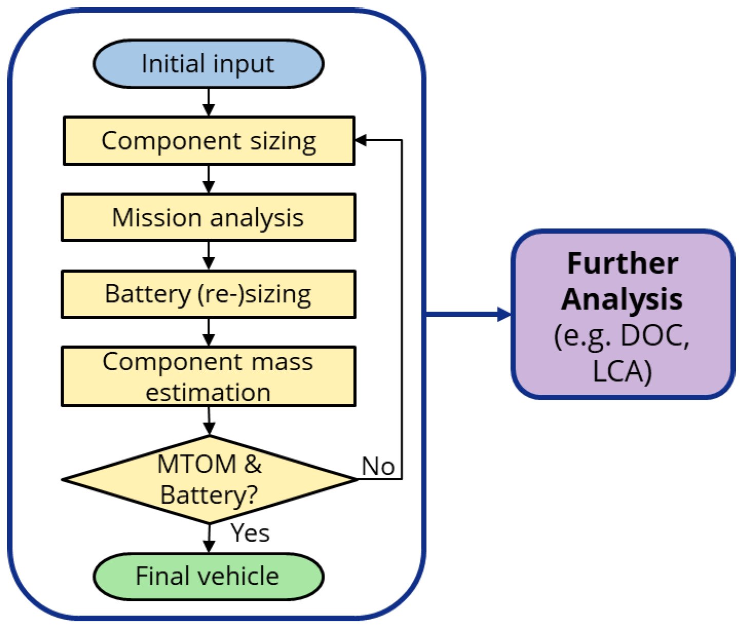
The overall sizing routine consists of four interconnected modules: component sizing, mission analysis, battery sizing, and mass estimation. Component sizing determines the characteristics of the major vehicle subsystems, while mission analysis evaluates the energy and power demands throughout the flight profile. Battery sizing ensures that sufficient onboard energy and power are available to satisfy mission requirements, and mass estimation updates the aircraft weight breakdown accordingly.

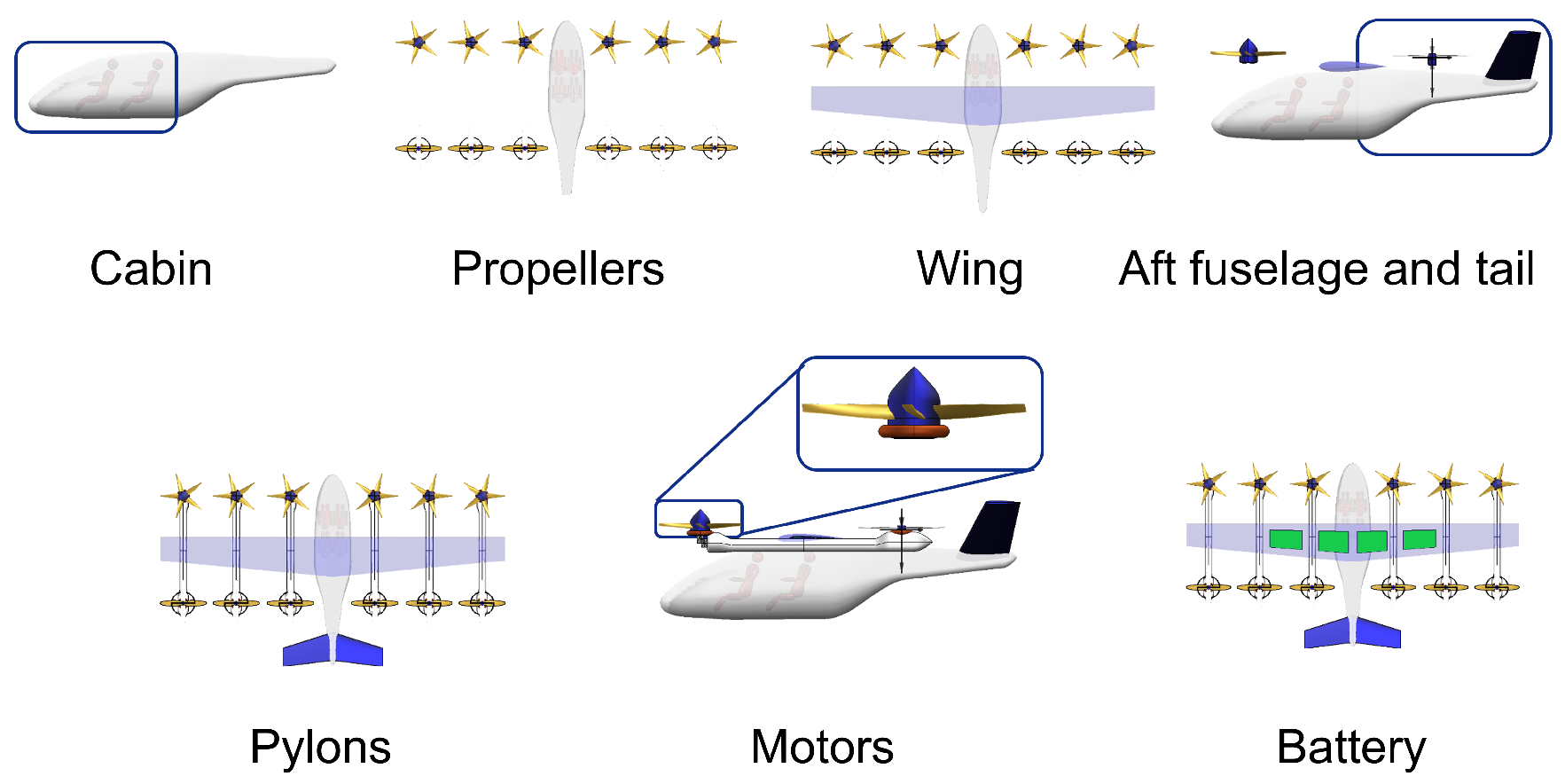
These modules are executed sequentially and repeated iteratively until convergence is achieved for both the maximum take-off mass (MTOM) and the battery capacity. An overview of the complete sizing and analysis framework is presented in Figure 1.

2.3. Component Sizing

The first step of the sizing routine is the aircraft component sizing. The corresponding procedure is illustrated in Figure 2. It uses a minimal set of initial inputs and sequentially determines either geometric parameters (such as fuselage and wing dimensions) or performance parameters (such as design motor power and torque ratings).

The procedure follows a sequential parameter enrichment approach. First, the cabin dimensions are determined, followed by the propeller and wing parameters. The aft fuselage and tailplane are then sized based on the previously obtained results. Subsequently, the motor pylon geometry and electric motor parameters, as well as the initial battery size, are calculated. The individual component sizing methods are described in more detail in the following subsections.

2.3.1. Fuselage (and Empennage)

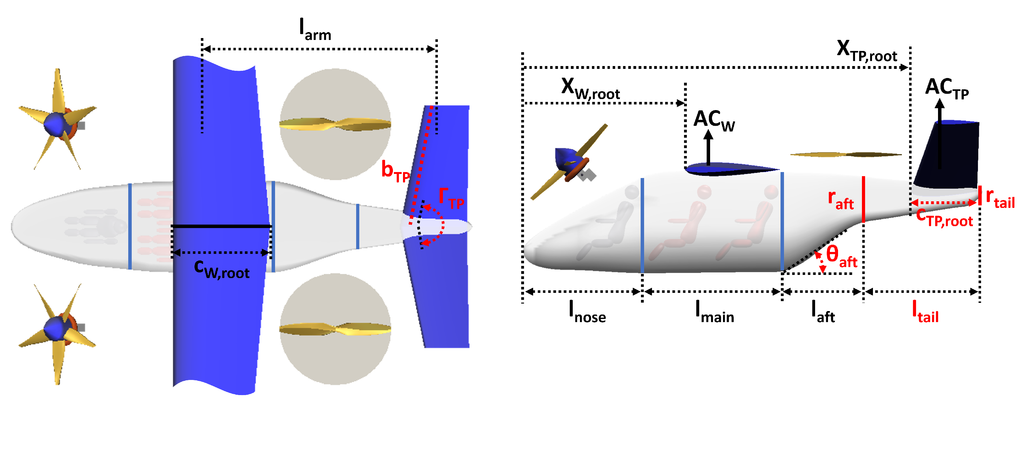
The fuselage is divided into four sections: the front (nose/cockpit), mid (cabin), aft, and tail sections as illustrated in Figure 3. The sections are approximated by simple geometric shapes, including elliptic paraboloid, elliptic cylinder, and elliptic frustum.

• Nose and cabin

The fuselage sizing process begins with the nose and cabin sections. The nose is approximated as an elliptic paraboloid, while the cabin is modeled as an elliptic cylinder. Their dimensions are derived from the number of occupants (pilots and passengers) and the predefined seat arrangement. Anthropometric data for both passengers and pilots is taken from [30]. For piloted configurations, an increased seat pitch is assumed, resulting in a longer nose/cockpit section. Cabin width and height are determined for occupants in a seated position, with an additional clearance margin of 5–10% applied to account for spacing to the fuselage walls.

• Rear fuselage and tailplane

Since both powered-lift configurations (such as Lift + Cruise, Tilt-Propeller, and Lift + Lift/Cruise) and wingless configurations can be modeled, the rear fuselage sizing procedure follows two distinct paths.

For multirotor configurations, no fuselage tail section is present. The aft fuselage is modeled as an oblique elliptic frustum. Its length is determined from the equivalent cabin diameter $D_{\mathrm{cabin}}$, the predefined taper ratio $r_{\mathrm{aft}}$ (typically in the range 0.2–0.3), and the aft cone angle ${\theta }_{\mathrm{aft}}$ (typically 30–45 degrees), resulting in

$$L_{\mathrm{aft}}={\displaystyle \frac{(1-r_{\mathrm{aft}}) D_{\mathrm{cabin}}}{tan\left({\theta }_{\mathrm{aft}}\right)}}$$

(1)

For winged aircraft configurations, the sizing of the rear fuselage and tailplane is formulated as a constrained optimization problem, as shown in Equation (2). The objective is to minimize the total wetted area $S_{\mathrm{wet},\mathrm{rear}}$, as defined in Equation (3).

The design variables for the optimization are shown in red in Figure 3. The fuselage unknowns are the aft taper ratio $r_{\mathrm{aft}}$, aft cone angle ${\theta }_{\mathrm{aft}}$, tail section length $l_{\mathrm{tail}}$, and tail section taper ratio $r_{\mathrm{tail}}$. The tailplane design variables are the root chord ($c_{\mathrm{TP},\mathrm{root}}$), half span ($b_{\mathrm{TP}}$), and dihedral angle (${\Gamma }_{\mathrm{TP}}$).

$$\begin{array}{cc}\hfill \mathrm{Minimize} & S_{\mathrm{wet},\mathrm{rear}}\left(\mathbf{X}\right)\hfill \\ \hfill \mathrm{w}.\mathrm{r}.\mathrm{t}. & \mathbf{X} = {\left[r_{\mathrm{aft}}, r_{\mathrm{tail}}, {\theta }_{\mathrm{aft}}, l_{\mathrm{tail}}, c_{\mathrm{TP},\mathrm{root}}, b_{\mathrm{TP}}, {\Gamma }_{\mathrm{TP}}, \right]}^{\mathsf{T}},\hfill \\ \hfill \mathrm{subject} \mathrm{to} & {\mathrm{V}}_{\mathrm{H}} \ge {\mathrm{V}}_{\mathrm{H},\min },\hfill \\ \hfill & {\mathrm{V}}_{\mathrm{V}} \ge {\mathrm{V}}_{\mathrm{V},\min },\hfill \\ \hfill & {\mathrm{x}}_{\mathrm{TP}} \ge {\mathrm{x}}_{\mathrm{W},\mathrm{root}}+{\mathrm{c}}_{\mathrm{W},\mathrm{root}}+{\mathrm{D}}_{\mathrm{prop}},\hfill \\ \hfill & {\mathrm{AR}}_{\mathrm{lower}} \le {\mathrm{AR}}_{\mathrm{TP}} \le {\mathrm{AR}}_{\mathrm{upper}},\hfill \\ \hfill & {\mathrm{r}}_{\mathrm{aft}} \ge {\mathrm{r}}_{\mathrm{tail}},\hfill \end{array}$$

(2)

where

$$S_{\mathrm{wet},\mathrm{rear}}=S_{\mathrm{fuse},\mathrm{aft}}+S_{\mathrm{fuse},\mathrm{tail}}+S_{\mathrm{TP}}$$

(3)

The optimization procedure is subject to several constraints. The first two are derived from the requirement for static stability of the aircraft, such that the horizontal and vertical tail volume coefficients are consistent with those of similar category aircraft. The tail volume coefficients are defined in Equation (4). Here, the driving parameters are the horizontal and vertical projected tail areas ($S_{\mathrm{HT}}$ and $S_{\mathrm{VT}}$), the wing mean aerodynamic chord $c_{\mathrm{w},\mathrm{mac}}$, the wing span $b_{\mathrm{w}}$, and the tail arm $l_{\mathrm{arm}}$, i.e., the longitudinal distance between the wing aerodynamic center and the tail aerodynamic center:

$$\begin{array}{cccc}\hfill \left(\mathrm{a}\right) V_H& ={\displaystyle \frac{S_{HT} l_{\mathrm{arm}}}{S_w c_{\mathrm{w},\mathrm{mac}}}}, \hfill & \hfill \left(\mathrm{b}\right) V_V& ={\displaystyle \frac{S_{VT} l_{\mathrm{arm}}}{S_w b_w}}.\hfill \end{array}$$

(4)

The third constraint ensures that the tailplane is positioned behind the aft propellers, where $x_{\mathrm{TP}}$ denotes the position of the tailplane root chord, $x_{\mathrm{W},\mathrm{root}}$ the position of the wing root chord, $c_{\mathrm{W},\mathrm{root}}$ the wing root chord length, and $D_{\mathrm{prop}}$ the diameter of the aft propellers. Further details on the determination of the propeller and wing parameters are provided in Section 2.3.2 and Section 2.3.3.

The last two constraints follow from the requirement that the rear fuselage must be converging, and that the tailplane aspect ratio remains within a prescribed range due to structural mass considerations.

2.3.2. Propeller

Three types of propellers are currently implemented: two dedicated to vertical take-off and landing (VTOL), namely lift-propellers and tilt-propellers, and a third type used exclusively for forward propulsion.

The primary design parameters for propeller sizing are the required thrust and the hover tip Mach number under specified design atmospheric conditions, defined by altitude and temperature offsets. The total hover thrust requirement, derived from the MTOM, is distributed among the VTOL propellers. In addition, a maneuvering margin of 10% is applied to the hover thrust requirement.

The main input parameters include the MTOM, landing pad footprint $L_{\mathrm{LP}}$, design cruise speed $V_{\mathrm{cruise},\mathrm{des}}$, design cruise lift coefficient $C_{\mathrm{L},\mathrm{cruise}}$, and fuselage width $W_{\mathrm{fuse}}$. Additional inputs comprise the design hover tip Mach number, number of blades $N_{\mathrm{b}}$, hub-to-tip ratio, induced power factor in hover ${\kappa }_{\mathrm{hover}}$, design altitude, temperature deviation from standard conditions, ratios of rotational speed in climb and cruise relative to hover, maximum speed ratio relative to cruise, and blade taper ratio t. While the tip Mach number in hover is used to define the rotational speed for the sizing procedure, the tip Mach number in forward flight can become a limiting design constraint, as compressibility effects at the blade tip must be avoided to maintain high aerodynamic efficiency. However, for powered-lift eVTOL configurations the maximum advance ratios remain low, since the aircraft is wing-borne in cruise flight, and the propellers operate on full load only during the transition. For conventional rotorcraft configurations, on the other hand, the tip Mach number at the highest forward flight speed should be explicitly considered when selecting the rotational speed to ensure that the critical Mach number is not exceeded.

The design thrust of each VTOL propeller is determined from the MTOM, number of VTOL propellers $N_{\mathrm{prop},\mathrm{VTOL}}$, and the maneuver factor $k_{\mathrm{maneuver}}$ as

$$T_{\mathrm{prop},\mathrm{des}}={\displaystyle \frac{k_{\mathrm{maneuver}} m_{\mathrm{MTO}} g}{N_{\mathrm{prop},\mathrm{VTOL}}}}.$$

(5)

The propeller radius is selected to be as large as possible within geometric constraints in order to minimize disk loading and, consequently, hover power. The maximum allowable radius is limited by the available landing pad footprint and the required spacing between propellers to avoid aerodynamic and acoustic interference. The propeller tip radius is therefore defined as

$$R_{\mathrm{tip}}=\left\{\begin{array}{cc}{\displaystyle \frac{1}{2}\frac{b_{\mathrm{eff}}}{(1+k_{\mathrm{lat}}) N_{\mathrm{prop},\mathrm{wing}}},}\hfill & (\mathrm{winged} \mathrm{configuration}),\hfill \\ {\displaystyle \frac{1}{4}\frac{b_{\mathrm{eff}}}{(1+k_{\mathrm{lat}})},}\hfill & (\mathrm{multirotor} \mathrm{configuration}),\hfill \end{array}\right.$$

(6)

where $k_{\mathrm{lat}}$ is the lateral spacing between propellers expressed as a fraction of the propeller diameter and $N_{\mathrm{prop},\mathrm{wing}}$ is the number of propellers per wing. The effective span available $b_{\mathrm{eff}}$ for propeller placement depends on the landing pad footprint $L_{\mathrm{LP}}$ and the fuselage width $W_{\mathrm{fuse}}$ and is given by

$$b_{\mathrm{eff}}=L_{\mathrm{LP}}-W_{\mathrm{fuse}}.$$

(7)

The propeller power is calculated using a combination of momentum theory and a simplified blade element approach, as detailed in [31,32]. The adopted formulation is intended for conceptual design studies and therefore neglects higher-order aerodynamic effects such as tip losses, rotor–wing and rotor–rotor interactions, non-uniform inflow, and unsteady transition-flight phenomena, which can be accounted for using correction coefficients. The total power is decomposed into induced and profile power components, as described in Section 2.4. The estimation of profile power requires the determination of propeller solidity.

• Propeller solidity and blade twist

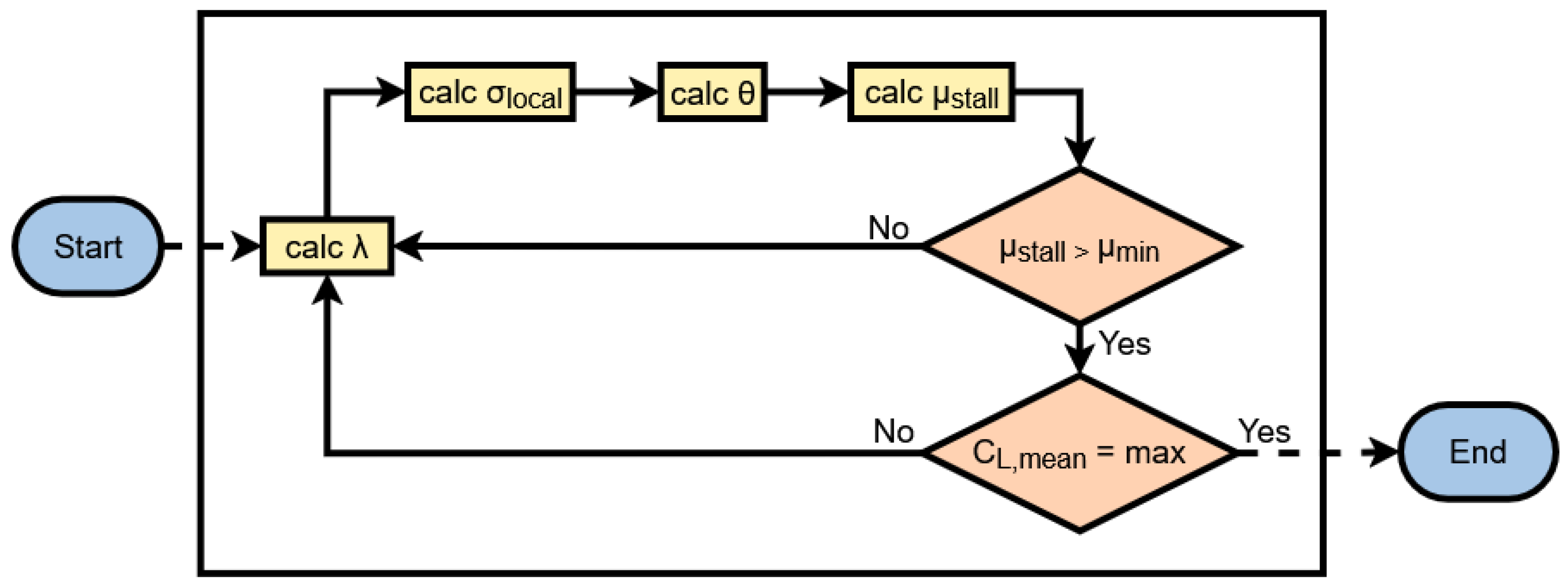
The propeller solidity is determined through an iterative procedure, as illustrated in Figure 4. The objective is to maximize the propeller disk mean lift coefficient $C_{\mathrm{L},\mathrm{mean}}$ in hover while ensuring that blade stall does not occur prior to reaching the design cruise speed for the rotorcraft, or, in the case of powered-lift configurations, the transition speed up to which the lifting propellers support the full aircraft weight. This requirement implies that the blade section lift coefficient must remain below the maximum lift coefficient of the airfoil across the entire operating envelope.

The first step is to determine the inflow ratio $\lambda$ in hover, which depends on the thrust coefficient $C_{\mathrm{T}}$. The thrust coefficient is calculated based on the required hover thrust, the predefined rotational speed $\omega$, and the propeller tip radius $R_{\mathrm{tip}}$. The rotational speed in hover is defined by the design tip Mach number $M_{\mathrm{tip}}$.

$$\begin{array}{cc}\hfill \lambda & =\sqrt{{\displaystyle \frac{C_T}{2}}}, C_T={\displaystyle \frac{T_{\mathrm{prop},\mathrm{des}}}{\rho \pi R_{\mathrm{tip}}^2{\left(\omega R_{\mathrm{tip}}\right)}^2}}, {\omega }_{\mathrm{hov}}={\displaystyle \frac{M_{\mathrm{tip}} a}{R_{\mathrm{tip}}}}.\hfill \end{array}$$

(8)

The next step is to determine the geometric parameters of the propeller blades. Each blade is linearly tapered, with the taper ratio specified by the user. While a higher-order twist distribution would yield lower induced power and thus improved performance, the requirement to rearrange the inflow ratio equation and solve for the unknown solidity using an analytical expression led to this formulation being selected and considered suitable for the initial stage of the vehicle design, as further propeller optimization is expected in subsequent design iterations using higher-fidelity methods. For a linearly tapered blade whose root begins at the nondimensional radius $r_0$, the local solidity distribution is defined as

$$\begin{array}{cc}\hfill {\sigma }_{\mathrm{root}}& ={\displaystyle \frac{4 {\sigma }_{\mathrm{mean}}}{\left(3-4r_0\right) \mathrm{t}+1+4r_0}},\hfill \\ \hfill {\sigma }_{0.75}& ={\sigma }_{\mathrm{root}}+(0.75-r_0) ({\sigma }_{\mathrm{tip}}-{\sigma }_{\mathrm{root}}).\hfill \end{array}$$

(9)

where the mean thrust-weighted solidity ${\sigma }_{\mathrm{mean}}$ is related to the design variable $C_{\mathrm{L},\mathrm{mean}}$ through

$${\sigma }_{\mathrm{mean}}={\displaystyle \frac{6 C_{\mathrm{T}}}{C_{\mathrm{L},\mathrm{mean}}}}.$$

(10)

The second geometric parameter to be obtained is the blade twist. The blade is assumed to have a linear twist distribution with an approximated linear inflow ratio. This allows the twist rate, ${\theta }_{\mathrm{rate}}$, to be derived analytically from [31]. The blade twist angles at the 75% radius, root, and tip are then computed using Equation (11). The aerodynamic characteristics of the airfoil, $c_{l_{\alpha }}$, are based on a representative rotor airfoil, such as the NACA 23012.

$$\begin{array}{cc}\hfill {\theta }_{75}& =3\left({\displaystyle \frac{2C_T}{{\sigma }_T{c}_{l_{\alpha }}}}+{\displaystyle \frac{\lambda }{2}}\right)\hfill \\ \hfill {\theta }_{\mathrm{root}}& ={\theta }_{75}-(0.75-r_0) {\theta }_{\mathrm{rate}}\hfill \\ \hfill {\theta }_{\mathrm{tip}}& ={\theta }_{\mathrm{root}}+(1-r_0) {\theta }_{\mathrm{rate}}\hfill \end{array}$$

(11)

The final step in the iterative blade design procedure is to determine the advance ratio, ${\mu }_{\mathrm{stall}}$, at which stall of the retreating blade occurs and significant power losses begin to arise, following the approach proposed by [33],

$$\begin{array}{cccc}\hfill {\mu }_{\mathrm{stall}}& =1-\sqrt{{\displaystyle \frac{C_{\mathrm{L},\mathrm{mean}}}{c_{l,max}}} {\displaystyle \frac{k}{3}}} \hfill & \hfill \mathrm{with} k& =3.17-2.7({\theta }_{\mathrm{tip}}-{\theta }_{\mathrm{root}})\hfill \end{array}$$

(12)

The design process is iterated by adjusting the solidity and blade twist until the mean lift coefficient, $C_{\mathrm{L},\mathrm{mean}}$, is maximized while satisfying the retreating-blade stall constraint, ${\mu }_{\mathrm{stall}}\ge {\mu }_{\mathrm{req}}$.

The required advance ratio, ${\mu }_{\mathrm{req}}$, is defined as

$${\mu }_{\mathrm{req}}=\begin{array}{c}\hfill {\displaystyle \frac{V_{\infty ,\mathrm{stall}}cos\alpha }{\omega R}}\end{array} \mathrm{with} \begin{array}{c}\hfill V_{\infty ,\mathrm{stall}}=\left\{\begin{array}{cc}{V}_{\mathrm{cruise},\mathrm{des}} {\left({\displaystyle \frac{C_{\mathrm{L},\mathrm{cruise}}}{C_{\mathrm{L},\max }}}\right)}^{0.5} \hfill & (\mathrm{winged} \mathrm{rotorcraft})\hfill \\ k_{\mathrm{stall}} V_{\mathrm{cruise},\mathrm{des}}\hfill & \left(\mathrm{multirotor}\right)\hfill \end{array}\right.\end{array}$$

(13)

where $V_{\infty ,\mathrm{stall}}$ represents the flight speed at which stall of the retreating blade occurs. For powered-lift configurations, this speed corresponds to the fixed-wing stall speed, estimated using the design cruise wing lift coefficient $C_{\mathrm{L},\mathrm{cruise}}$ and the wing airfoil’s maximum lift coefficient $C_{\mathrm{L},\max }$. For multirotor configurations, it is obtained by applying a margin factor $k_{\mathrm{stall}}$ above the design cruise speed, typically in the range 1.05–1.10.

2.3.3. Wing

The wing is designed for cruise flight and features a trapezoidal planform. The wingspan b depends on the vehicle configuration, but is constrained by the landing pad dimensions. It may be set equal to the landing pad length $L_{\mathrm{LP}}$, or, if wingtip propellers are used, reduced by the radius of the tip propellers on both sides.

The procedure uses several user-defined parameters, such as the wing thickness-to-chord ratio $t/c$ (typically 18–20% due to structural and battery volume requirements), leading-edge sweep ${\mathsf{\Lambda }}_{\mathrm{LE}}$, dihedral angle $\Gamma$, and taper ratio $\lambda$. The atmospheric design conditions, i.e., design altitude and temperature, are also specified.

The remaining geometric parameters, including root, tip, and mean chords, are obtained through an optimization procedure that minimizes the portion of cruise power attributable to the wing. The design variable is the cruise lift coefficient $C_{\mathrm{L},\mathrm{cruise}}$, which is adjusted to maximize the lift-to-drag ratio while minimizing wing mass, subject to constraints on aspect ratio and the required maneuvering capability (e.g., sustaining a ${60}^{\circ }$ banked turn during cruise).

The optimization problem is formulated as

$$\begin{array}{cc}\hfill \mathrm{Minimize} & P_{\mathrm{wing}}\left(C_{\mathrm{L},\mathrm{cruise}}\right)\hfill \\ \hfill \mathrm{subject} \mathrm{to} & {\mathrm{C}}_{\mathrm{L},\max } \ge {\displaystyle \frac{2 n m_{\mathrm{MTO}}}{\rho V_{\infty }^2 S_{\mathrm{ref}}}},\hfill \\ \hfill & {\mathrm{AR}}_{\mathrm{lower}} \le {\mathrm{AR}}_{\mathrm{wing}} \le {\mathrm{AR}}_{\mathrm{upper}},\hfill \end{array}$$

(14)

The objective function is formulated to minimize the cruise drag power related to the wing $P_{\mathrm{wing}}$, accounting for the trade-off between its aerodynamic efficiency and structural weight. On the one hand, reducing the wing area and increasing the aspect ratio improves the lift-to-drag ratio. On the other hand, higher wing loading and aspect ratio increase the wing mass, which in turn raises the total aircraft weight. This balance is captured by the following expression:

$$P_{\mathrm{wing}}\left(C_{\mathrm{L},\mathrm{cruise}}\right)=\left(1+{\displaystyle \frac{m_{\mathrm{wing}}}{m_{\mathrm{MTO}}}}\right){\displaystyle \frac{C_{\mathrm{D},\mathrm{tot}}}{C_{\mathrm{L},\mathrm{cruise}}}}.$$

(15)

The wing mass is estimated using the Cessna semi-empirical relation [34] as a function of maximum take-off mass $m_{\mathrm{MTO}}$ (lb), aspect ratio $AR$, and reference wing area $S_{\mathrm{ref}}$ (ft²):

$$m_{\mathrm{wing}}=0.04674 {(3.8 m_{\mathrm{MTO}})}^{0.398} S_{\mathrm{ref}}^{0.360} A{R}^{1.172}.$$

(16)

Wing drag is calculated using the drag build-up method described in Section 2.4 (see Equations (19), (20) and (22)). Since the drag contributions of other components are not yet known at this stage, the wing parasitic drag is assumed to represent approximately one-third of the total parasitic drag for this type of vehicle.

2.3.4. Pylon

The pylons supporting the VTOL propellers can be represented either as tubular (cylindrical) structures or as wing-shaped lifting surfaces, depending on the vehicle configuration. Their dimensions are scaled proportionally to either the propeller hub or motor diameter.

A simple parametric relation is used to define the pylon length:

$$\begin{array}{c}\hfill L_{\mathrm{pylon}}=\left\{\begin{array}{cc}(1+2k_{\Delta })R_{tip} +0.5 c_{\mathrm{w},\mathrm{mean}} \hfill & (\mathrm{short} \mathrm{booms})\hfill \\ 2 (1+2k_{\Delta })R_{tip} + c_{\mathrm{w},\mathrm{mean}} \hfill & (\mathrm{long} \mathrm{booms})\hfill \\ y_{\mathrm{rotor}}sec(\pi /4)\hfill & \left(\mathrm{Quadrotor}\right)\hfill \end{array}\right.\end{array}$$

(17)

Here, $k_{\Delta }$ represents the distance between the propeller and the wing as a fraction of the propeller diameter, $R_{\mathrm{tip}}$ is the propeller radius, and $c_{\mathrm{w},\mathrm{mean}}$ is the mean chord of the wing. The span-wise locations of the motors are obtained from the propeller layout.

2.3.5. Electric Motor

The electric motor diameter is assumed to be equivalent to the propeller hub diameter. Motor sizing is carried out by evaluating three flight conditions: hover, climb, and cruise. For each of these conditions, the relevant performance parameters, thrust T, power P, and rotational speed $\omega$, are computed based on the vehicle configuration and the propeller type. In hover, a thrust increase of 10% is included to account for maneuvering. For climb, the design-point conditions are assumed to include a specific rate of climb at the top of climb.

These performance parameters define the motor ratings, namely the maximum continuous power (MCP), maximum rated power (MRP), and contingency rated power (CRP), along with their corresponding torque values. The specific definition of these ratings depends on the propeller type, as summarized in

Table 1. Motor power ratings for the different propeller types.

Propeller Type	MCP	MRP	CRP
Tilt-propeller	Cruise	Hover	Hover OEI
Lift-propeller (winged)	Hover	Hover	Hover OEI
Lift-propeller (wingless)	Cruise	Hover	Hover OEI
Forward propeller	Cruise	Climb	Climb OEI

. These maximum ratings are needed for selecting a motor capable of meeting performance requirements across all flight conditions and for estimating its mass, as described in Section 2.6.3.

The motor sizing process accounts for both all-propellers/all-motors-operative conditions and motor/propeller failure conditions, also referred to as one-engine-inoperative (OEI). In OEI scenarios, depending on the configuration, an opposing motor may be deactivated to maintain vehicle stability. This leads to an increase in the required thrust and, consequently, the required power per remaining motor. For configurations with a larger number of lifting propellers, this effect is less pronounced.

2.4. Mission Performance Analysis

• Mission definition and analysis

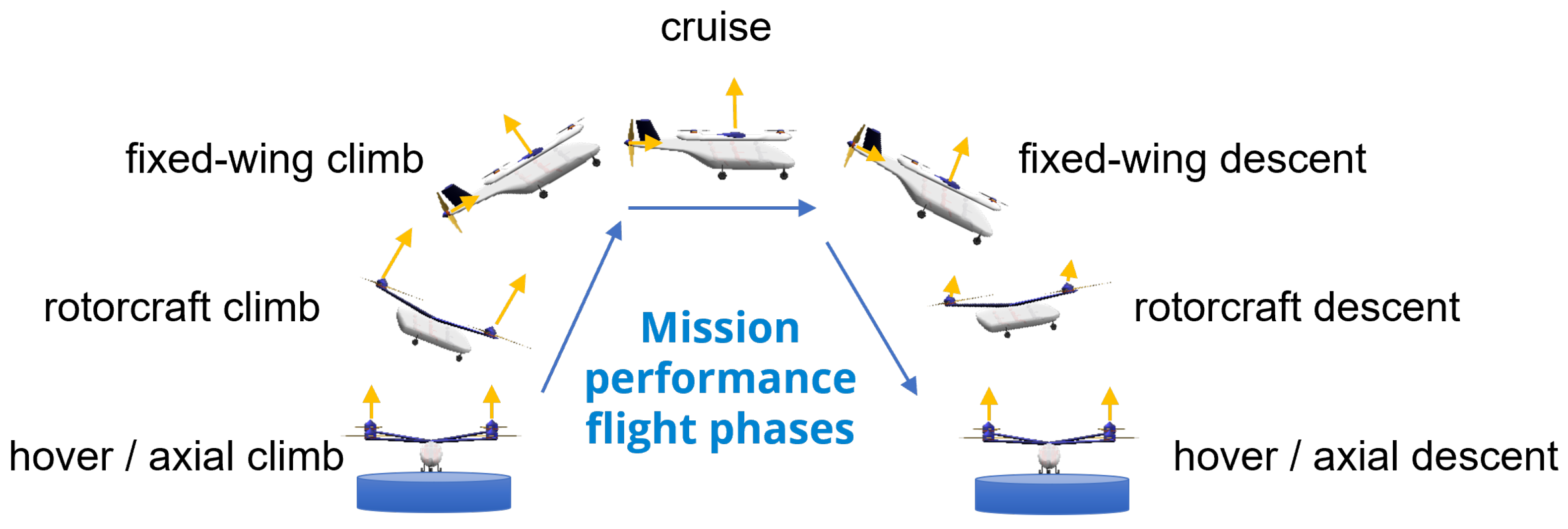
The mission analysis incorporates a dedicated module to calculate the vehicle performance across different mission profiles (including multi-leg operation), covering both vertical and forward flight. The mission is defined as a sequence of several types of flight phases, as illustrated in Figure 5.

Four types of flight segments are considered. The hover and axial climb/descent segment represents purely vertical flight, encompassing stationary hover and climb or descent with only axial (vertical) velocity. The rotorcraft climb/descent segment involves horizontal acceleration or deceleration combined with a change in altitude, with lift generated exclusively by the propellers/rotors, while during the fixed-wing climb or descent segment, lift is generated solely by lifting surfaces. The cruise segment models steady forward flight (both rotorcraft and fixed-wing) at constant speed and altitude.

For each segment, altitude, speed, climb or descent rate, range, or duration are specified. Each segment is discretized into $N_{\mathrm{cp}}$ steady-state control points, which provide sufficient temporal and spatial resolution to evaluate the vehicle performance throughout the mission. At each control point, the atmospheric and flight conditions are computed, and a set of force-balance equations is solved to determine the required thrust, aerodynamic forces, and propeller power.

The governing force-balance equations for the different flight segments are given by

$$\begin{array}{cc}\begin{array}{cc}\hfill T& =m_{\mathrm{TO}} g_0\hfill \end{array} \hfill & (\mathrm{hover}, \mathrm{axial} \mathrm{climb}/\mathrm{descent})\hfill \\ \left.\begin{array}{cc}\hfill Tcos\left(\alpha -\gamma \right)& =W+D sin\gamma \hfill \\ \hfill Tsin\left(\alpha -\gamma \right)& =D cos\gamma -{\displaystyle \frac{W}{g_0}} a_x\hfill \end{array}\right\} \hfill & (\mathrm{rotorcraft} \mathrm{climb}/\mathrm{descent})\hfill \\ \begin{array}{cc}\hfill T& =D_i + m_{\mathrm{TO}}\left(g_0 sin{\gamma }_i + a\right)\hfill \end{array} \hfill & (\mathrm{fixed}-\mathrm{wing} \mathrm{climb}/\mathrm{descent}/\mathrm{cruise})\hfill \end{array}$$

(18)

For hover and axial climb or descent, the required thrust equals the vehicle weight, where $m_{\mathrm{TO}}$ is the take-off mass and $g_0$ is the gravitational acceleration at sea level.

For rotorcraft climb and descent, the required thrust T and propeller disk incidence angle $\alpha$ are functions of the take-off mass $m_{\mathrm{TO}}$, horizontal acceleration $a_x$, climb angle $\gamma$, and aerodynamic drag force D. These quantities are obtained by solving the system in Equation (18) using a numerical root-finding method.

In the fixed-wing climb, descent, and cruise segments, the required thrust is determined from the take-off mass $m_{\mathrm{TO}}$, the flight path angle $\gamma$, and the acceleration a.

The present implementation relies on simplified aerodynamic representations and force-balance formulations that are intended for conceptual design studies; stability and control derivatives are not currently evaluated. Future developments could incorporate semi-empirical methods from aerodynamic prediction tools, such as the USAF Stability and Control Digital DATCOM [35], to provide better lift, drag, and moment coefficient estimates as well as stability derivatives for powered-lift configurations. Such an approach would improve the fidelity of the aerodynamic model while maintaining computational efficiency suitable for early-stage design exploration.

• Drag build-up

The aerodynamic drag is estimated using the drag build-up approach in [30], in which the total drag coefficient is decomposed into induced and parasitic drag:

$$C_D=C_{D_i}+C_{D_0}$$

(19)

The induced drag coefficient is computed as

$$\begin{array}{cccc}\hfill C_{D_i}& ={\displaystyle \frac{1}{\pi e AR}} C_L^2 \hfill & \hfill \mathrm{with} e& =1.78 (1-0.045 A{R}^{0.68})-0.64\hfill \end{array}$$

(20)

where e is the Oswald efficiency factor [36] and $AR$ is the wing aspect ratio.

The parasitic drag coefficient is obtained from a component-wise build-up method:

$$\begin{array}{cc}\hfill C_{D_0}=[& c_{d,\mathrm{wing}}+c_{d,\mathrm{tail}}+c_{d,\mathrm{fuse}}+c_{d,\mathrm{LG}}\hfill \\ & +c_{d,\mathrm{pyl}} N_{\mathrm{pyl}}+\left(c_{d,\mathrm{blade}}+c_{d,\mathrm{hub}}\right) N_{\mathrm{liftprop}}] k_{\mathrm{CRUD}}\hfill \end{array}$$

(21)

where $k_{\mathrm{CRUD}}$ is a correction factor accounting for the cumulative result of undesirable drag [30].

The parasitic drag coefficient of each component (wing, tail, fuselage, landing gear, pylons, blades, hubs) is calculated as

$$\begin{array}{cccc}\hfill C_{D,\mathrm{comp}}& ={\displaystyle \frac{S_{\mathrm{wet}}}{S_{\mathrm{ref}}}} \left(c_f FF IF\right) \hfill & \hfill \mathrm{with} c_f& ={\displaystyle \frac{0.455}{{\left({log}_{10} \left(\mathrm{Re}\right)\right)}^{2.58}{\left(1+0.144 \frac{V_{\infty }}{a^2}\right)}^{0.65}}}\hfill \end{array}$$

(22)

Here, $S_{\mathrm{wet}}$ is the wetted area, $S_{\mathrm{ref}}$ the reference area, $FF$ the form factor, $IF$ the interference factor, and $c_f$ the skin friction coefficient. The Reynolds number $\mathrm{Re}$ is based on a characteristic length of the component, $V_{\infty }$ is the freestream velocity, a is the speed of sound, and $\mu$ is the dynamic viscosity. A fully turbulent flow is assumed, which provides conservative drag estimates.

The form factor $FF$ for wing, tail, fuselage, and pylons is taken as the average of methods proposed in [36,37,38,39,40].

The landing gear drag is estimated using empirical correlations representative of general aviation aircraft. The streamlined landing gear type I2 is assumed for the main gear and type M2 for the nose gear, similar to Cirrus SR-22 [30]:

$$c_{d,\mathrm{LG}}={\displaystyle \frac{\left(D_{\mathrm{tire}} W_{\mathrm{tire}}\right)}{S_{\mathrm{ref}}}} \Delta C_{D_s}$$

(23)

The tire diameter and width are determined following [36]

$$\begin{array}{cccc}\hfill D_{\mathrm{tire}}& =0.051 W_W^{0.349} \hfill & \hfill and W_{\mathrm{tire}}& =0.023 W_W^{0.312}\hfill \end{array}$$

(24)

where $W_W$ is the weight on the wheel and $D_{\mathrm{tire}}$ and $W_{\mathrm{tire}}$ are given in meters.

• Propeller power calculation

The total thrust required at each control point along the mission, obtained from the force-balance equations (see Equation (18)), is distributed among the active propellers at this flight condition.

For each propeller, power and torque are computed using a propeller performance model, as a function of required thrust $T_{prop}$, propeller angular velocity ${\omega }_p$, disk inflow velocity $V_{\mathrm{disk}}$, the freestream velocity, $V_{\infty }$, the disk incidence angle ${\alpha }_{\mathrm{disk}}$ and air density $\rho$:

$$P_{prop} ,Q_{prop}=f\left(T_{prop},V_{\mathrm{disk}},V_{\infty },{\alpha }_{\mathrm{disk}},\omega , \rho \right)$$

(25)

The propeller power is decomposed into induced and profile components:

$$P_{\mathrm{prop}}=\kappa T \left(v_i+V_z\right)+\rho A_d {\left(\omega R\right)}^3 C_{P0}$$

(26)

The induced power is computed using momentum theory with a correction for non-uniform inflow, where $\kappa$ is the induced power factor (typically $\kappa \approx 1.15$ for rotorcraft), $v_i$ is the induced velocity, and $V_z$ is the axial inflow velocity at the propeller disk.

The profile power is estimated based on blade element momentum theory (BEMT), where $A_d$ is the disk area, $\omega$ the rotational speed, R the propeller radius, and $C_{P0}$ the profile power coefficient.

The profile power coefficient is given by

$$C_{P0}={\displaystyle \frac{1}{8}} \sigma C_{d,\mathrm{mean}} F_{\mathrm{P}}$$

(27)

where $\sigma$ is the propeller solidity and $C_{d,\mathrm{mean}}$ is the mean sectional drag coefficient, approximated from the airfoil drag polar. The factor $F_{\mathrm{P}}$ accounts for the effect of combined edge-wise and axial inflow on the blade section velocity [14,41]. It is computed as

$$\begin{array}{cc}\hfill F_{\mathrm{P}} & =\sqrt{1+{\mu }_{\mathrm{tot}}^2}\left[1+{\displaystyle \frac{5}{2}}{\mu }_{\mathrm{tot}}^2+{\displaystyle \frac{3}{8}}{\mu }^2{\displaystyle \frac{4+7{\mu }_{\mathrm{tot}}^2+4{\mu }_{\mathrm{tot}}^4}{{(1+{\mu }_{\mathrm{tot}}^2)}^2}}-{\displaystyle \frac{9}{16}}{\displaystyle \frac{{\mu }^4}{1+{\mu }_{\mathrm{tot}}^2}}\right]\hfill \\ \hfill & +\left({\displaystyle \frac{3}{2}}{\mu }_z^4+{\displaystyle \frac{3}{2}}{\mu }_z^2{\mu }^2+{\displaystyle \frac{9}{16}}{\mu }^4\right)ln\left({\displaystyle \frac{\sqrt{1+{\mu }_{\mathrm{tot}}^2}+1}{{\mu }_{\mathrm{tot}}}}\right)\hfill \end{array}$$

(28)

where the advance ratios are defined as follows:

$$\begin{array}{cccccc}\hfill \mu & ={\displaystyle \frac{V_{\infty }cos\varphi }{\omega R}},\hfill & \hfill {\mu }_z& ={\displaystyle \frac{V_{\infty }sin\varphi }{\omega R}},\hfill & \hfill {\mu }_{\mathrm{tot}}& =\sqrt{{\mu }^2+{\mu }_z^2}\hfill \end{array}$$

(29)

Finally, the total shaft power required, accounting for propulsion system efficiencies, is given by

$$P_{\mathrm{shaft}}={\displaystyle \frac{P_{\mathrm{prop}}}{{\eta }_{\mathrm{motor}} {\eta }_{\mathrm{elec}}}}$$

(30)

The results of all mission segments are aggregated into a comprehensive mission dataset and form the power demand for the subsequent battery sizing. The resulting performance data is recorded for each segment and used for subsequent analyses, such as energy consumption estimation and battery sizing.

2.5. Battery Sizing

• Battery model and initial sizing

The method of determining the battery size (i.e., the number of battery cells) is based on the power demand along the mission profile, which is obtained from the mission performance analysis. The battery is modeled as a pack composed of multiple modules, each containing electrically connected, identical cells. The characteristics of each cell are defined by a nominal voltage $V_{\mathrm{cell},\mathrm{nom}}$, nominal capacity $C_{\mathrm{cell},\mathrm{nom}}$, maximum voltage $V_{\mathrm{cell},\max }$, cutoff voltage $V_{\mathrm{cut}-\mathrm{off}}$, and discharge-rate-dependent internal resistance $R_{\mathrm{tot}}$, which is derived from the discharge characteristics.

The sizing process is initiated using a mass-based relation and a nominal electrical architecture. The initial estimate of the usable pack energy is computed as

$$E_{\mathrm{batt},\mathrm{init}}={\displaystyle \frac{ϵ}{1+{\delta }_{\mathrm{pack}}}} f_{\mathrm{bat}} m_{\mathrm{MTO}},$$

(31)

where $ϵ$ is the cell gravimetric energy density, ${\delta }_{\mathrm{pack}}$ is the pack overhead factor accounting for the structural housing and thermal management, $f_{\mathrm{bat}}$ is the battery mass fraction, and $m_{\mathrm{MTO}}$ is the maximum take-off mass.

For a specified nominal bus voltage $V_{\mathrm{batt},\mathrm{nom}}$, the required number of cells in series $n_{\mathrm{s}}$ and in parallel $m_{\mathrm{p}}$ is determined as follows:

$$\begin{array}{cccc}\hfill n_s& ={\displaystyle \frac{V_{\mathrm{batt},\mathrm{nom}}}{V_{\mathrm{cell},\mathrm{nom}}}} \hfill & \hfill \mathrm{and} m_p& ={\displaystyle \frac{E_{\mathrm{batt}}}{n_s V_{\mathrm{cell},\mathrm{nom}} C_{\mathrm{cell},\mathrm{nom}}}}.\hfill \end{array}$$

(32)

• Overall battery sizing procedure

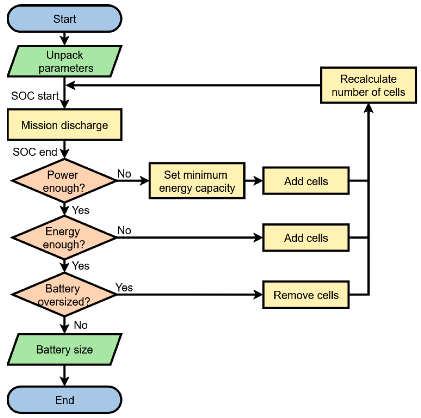
The overall battery sizing procedure is formulated as an iterative loop that ensures both power and energy requirements are satisfied over the entire mission profile, as shown in Figure 6. The process begins with defined cell and pack parameters of the initialized battery, along with the mission power demand profile and the state-of-charge (SOC) limits.

At each operational point, the total power required, consisting of the propulsion power and the motor and power electronics losses, is applied as a load to the battery system. The distribution of power demand across all cells is such that the power per cell is given by

$$P_{\mathrm{demand},\mathrm{cell}}={\displaystyle \frac{P_{\mathrm{demand},\mathrm{tot}}}{n_s m_p}}.$$

(33)

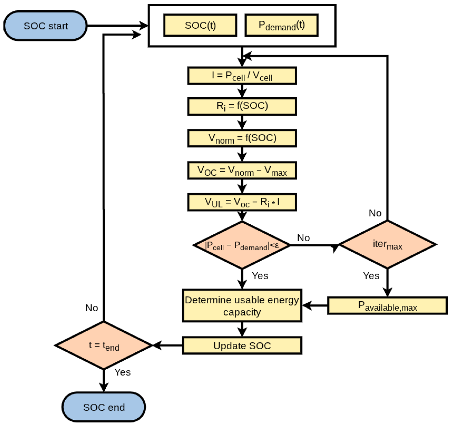
The behavior of each cell is analyzed using a discharge model that approximates the battery cell as a simplified equivalent circuit comprising a voltage source and an internal resistance network. The model focuses on electrical performance and does not explicitly account for thermal effects, battery aging, cell balancing, or degradation mechanisms. The procedure, illustrated in Figure 7, is based on the models presented by Vratny [42] and Chen [43]. Further details of the model are provided later in this subsection.

The analysis is carried out sequentially for the entire mission profile, with the state of charge being updated at each time step. At the end of each iteration, the maximum deliverable power, which is limited by the maximum discharge C-rate, is compared to the required power, and the minimum battery capacity is adjusted if necessary. In addition, the final state of charge is compared to the target value, and the battery size is increased or reduced accordingly. The procedure is repeated until a convergence tolerance of 1% is met.

• Cell discharge equivalent circuit

The cell discharge model evaluates the equivalent circuit at each operating point of the mission power demand profile by iteratively solving Ohm’s law, as illustrated in Figure 7. For a given instantaneous cell power demand, the current is obtained from

$$\begin{array}{cccccc}\hfill I& ={\displaystyle \frac{P_{\mathrm{demand},\mathrm{cell}}}{V_{UL}}} \hfill & \hfill \mathrm{with} V_{UL}& =V_{\mathrm{OC}}-R_{\mathrm{tot}} I \hfill & \hfill \mathrm{and} V_{\mathrm{OC}}& =V_{\mathrm{norm}} V_{max}\hfill \end{array}$$

(34)

where $V_{\mathrm{UL}}$ denotes the voltage under load, $V_{\mathrm{OC}}$ is the open-circuit voltage at the given state of charge, and $R_{\mathrm{tot}}$ represents the internal resistance. The normalized voltage $V_{\mathrm{norm}}$ is defined as the ratio of the discharge voltage at C/5 (0.6 A) to the maximum cell voltage. The internal resistance is derived from measured discharge characteristics at 0.6 A, 3 A, 10 A, and 20 A and interpolated to the instantaneous current, thereby capturing its dependence on both SOC and C-rate. The corresponding discharge curves for the Murata VTC6 cell, used for the verification cases in Section 3.2 and Section 3.3, are provided in [44].

The iterative solution is continued until the provided electrical power ($V_{UL} I$) matches the required $P_{demand,cell}$. If convergence is not achieved within a prescribed number of iterations, or if the resulting current exceeds the maximum allowable C-rate, the operating point is considered infeasible for the given battery. The maximum instantaneous cell power is evaluated as

$$\begin{array}{cccc}\hfill P_{\mathrm{cell},\max }& =V_{\mathrm{OC}} I_{max}-R_{\mathrm{tot}} I_{max}^2 \hfill & \hfill \mathrm{with} I_{max}& =C_{\mathrm{rate},\max } I_{\mathrm{nom}},\hfill \end{array}$$

(35)

where $I_{\mathrm{nom}}$ is the nominal cell current corresponding to $C_{\mathrm{cell},\mathrm{nom}}$.

Once convergence is achieved, the state of charge is updated using Coulomb counting:

$$\begin{array}{cccc}\hfill SO{C}_{i+1}& =SO{C}_i-{\displaystyle \frac{I_i \Delta t_i}{C_{\mathrm{act}}}} \hfill & \hfill \mathrm{with} C_{\mathrm{act}}& ={\displaystyle \frac{C_{\mathrm{cell},\mathrm{nominal}}}{C_{\mathrm{rel}}}},\hfill \end{array}$$

(36)

where $C_{\mathrm{act}}$ represents the effective available capacity. The factor $C_{\mathrm{rel}}$ denotes the relative capacity, accounting for C-rate-dependent capacity variations, and is derived from the adopted discharge model [42,43].

2.6. Estimation of Vehicle Mass

2.6.1. Overall Mass Breakdown

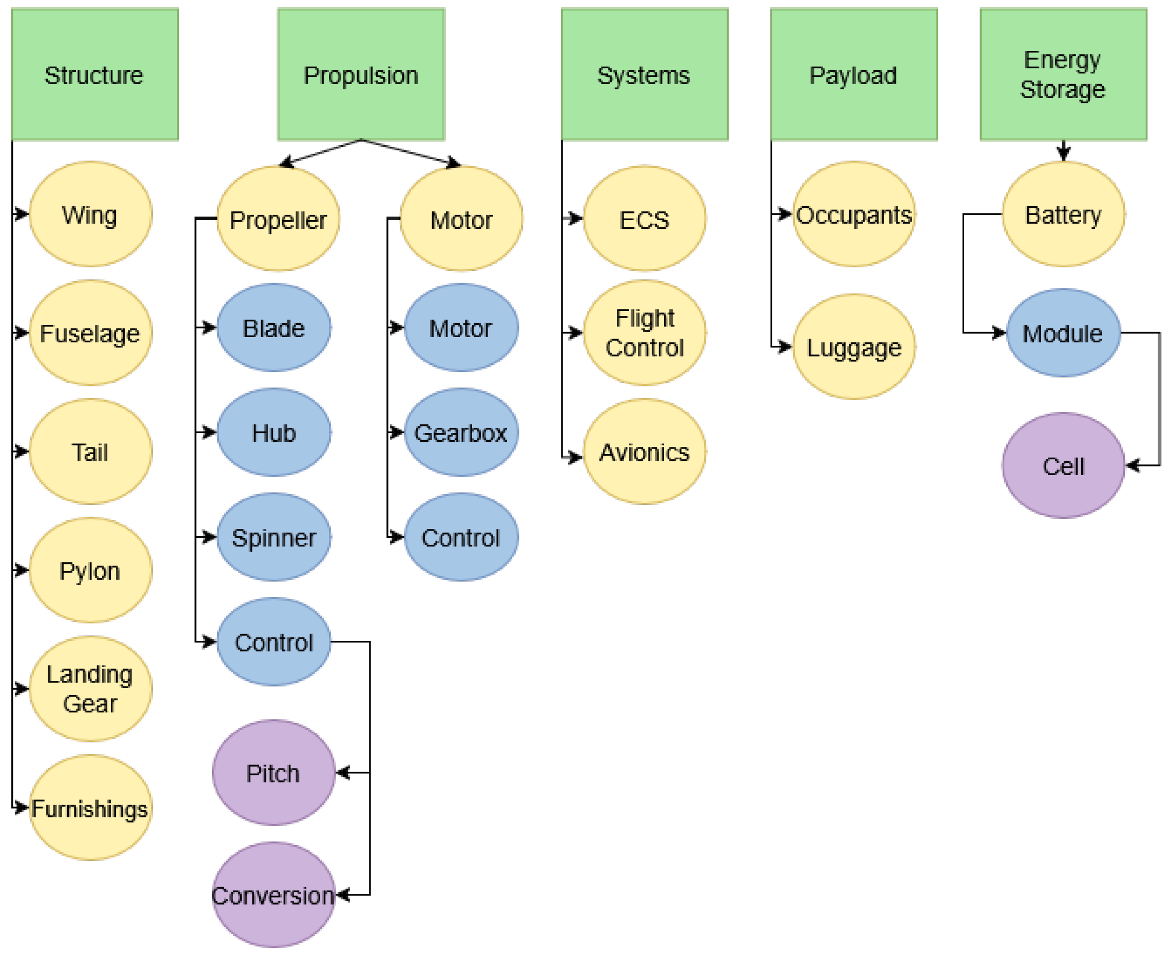
For the estimation of the vehicle mass, a component-based method is implemented. In this approach, the total mass is decomposed into a set of individual components, each of which is evaluated using either physics-based formulations or semi-empirical correlations, as illustrated in Figure 8.

The total mass $m_{\mathrm{total}}$ is defined as the sum of all individual component masses:

$$m_{\mathrm{total}}={\displaystyle \sum _{i=1}^N}{m}_i,$$

(37)

where $m_i$ denotes the mass of each component. The components are grouped into several main categories. The structure group comprises the primary airframe elements, including the wing, fuselage, tail, pylon, landing gear, and furnishing. The propulsion group includes the propeller and motor, along with their respective subcomponents. The systems group encompasses the environmental control system, flight control system, and avionics. The payload is subdivided into occupants (pilot and passengers) and luggage. Finally, the battery is modeled as an assembly of modules containing electrically interconnected cells.

2.6.2. Structure

• Wing and tail

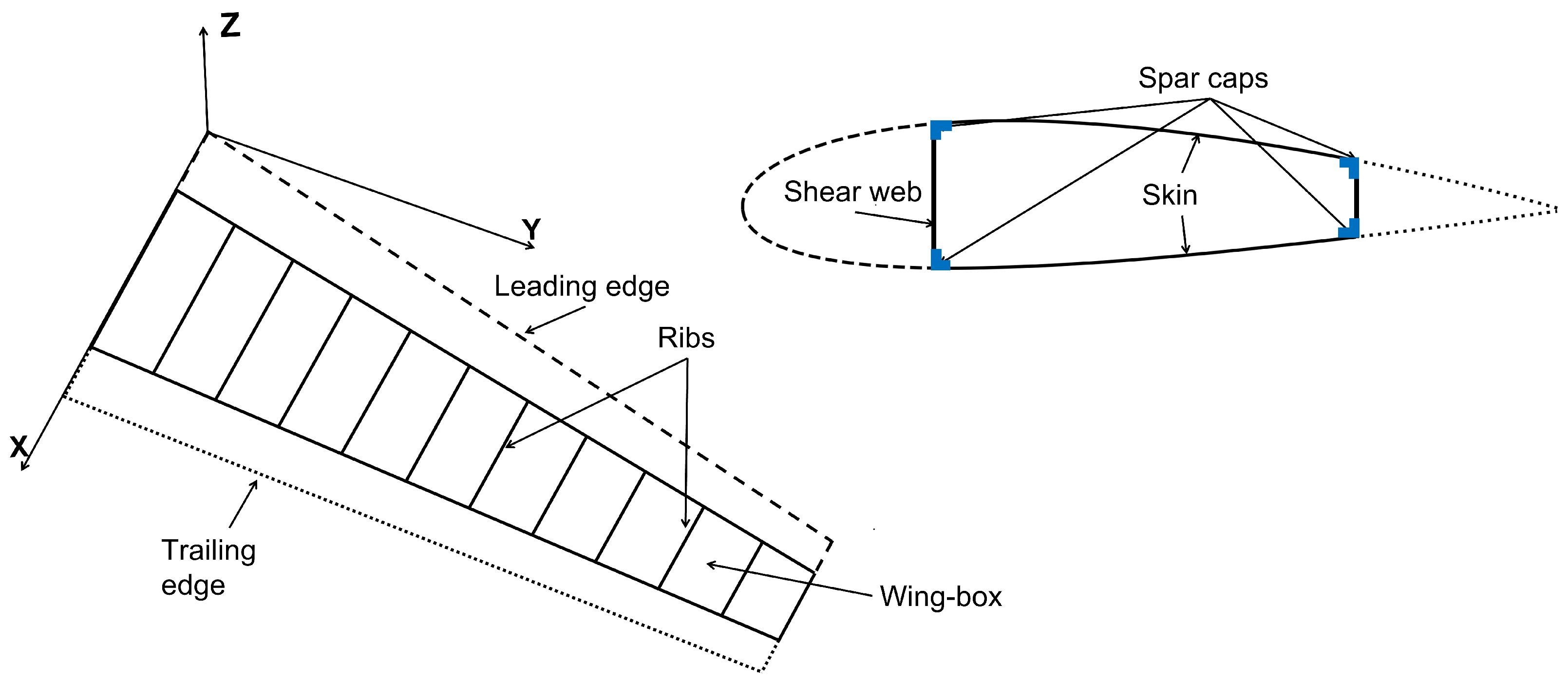
The mass of the wing and empennage is estimated using a physics-based formulation derived from the SUAVE framework [17] and adapted for composite structures, consistent with the conceptual structural assumptions of the Vahana project [45,46]. The estimation follows a structural build-up method based on conceptual design loads and simplified geometry assumptions. In this approach, the wing is represented as a load-carrying wingbox composed of spars, stressed skin, and discrete ribs, complemented by secondary, non-load-carrying components distributed along the span, as illustrated in Figure 9.

The sizing procedure determines the contributions from the torsion box, bending and drag caps, shear webs, leading- and trailing-edge surfaces, ribs, and external coating. Structural loads are computed from the Schrenk span-wise lift distribution [47], and are integrated numerically along the span to obtain shear forces and bending/torsion moments. All structural thicknesses are sized to satisfy ultimate failure loads or, for the non-lifting surfaces, the minimum gauge requirements. The total design load incorporates the limit load factor for a general aviation aircraft of $3.8$ with a safety factor of $1.5$ [48].

The wing geometry is derived from the vehicle definition and includes the projected wingspan b, mean aerodynamic chord c, thickness-to-chord ratio $t/c$ (approximated from a NACA four-digit equivalent airfoil), wing area S, forward and aft spar web locations $x_{\mathrm{fwd}},x_{\mathrm{aft}}$, and the shear center location $x_{\mathrm{SC}}$. The primary structure is sized according to the span-wise load distribution and geometric characteristics, while secondary, non-load-carrying elements are included as additional mass contributions.

The total wing mass is obtained by integrating the span-wise mass distribution of the primary structure and adding the contributions of the ribs, while a correction factor $k_{\mathrm{corr}}=1.2$ accounts for unmodeled effects and uncertainties:

$$m_{\mathrm{wing}}=k_{\mathrm{corr}}\left(2{\int }_0^{b/2}\left(\delta m_{\mathrm{wingbox}}+\delta m_{\mathrm{nonlift}}\right)\mathrm{d}y+m_{\mathrm{rib}} n_{\mathrm{ribs}}\right),$$

(38)

Within the wingbox formulation, the structural mass per unit span is composed of contributions from torsion, bending in both the y- and x- directions, and shear loads:

$$\delta m_{\mathrm{wingbox}}=\delta m_{\mathrm{torsion}}+\delta m_{\mathrm{My}}+\delta m_{\mathrm{Mx}}+\delta m_{\mathrm{shear}}$$

(39)

In addition to the load-carrying structure, non-lifting components such as leading- and trailing-edge surfaces and surface coatings contribute to the overall mass:

$$\delta m_{\mathrm{nonlift}}=\delta m_{\mathrm{LE}}+\delta m_{\mathrm{TE}}+\delta m_{\mathrm{paint}}$$

(40)

• Pylons

The pylons on which the lift propellers are mounted can be represented either as tubular (circular) structures or as wing-like lifting surfaces, depending on the vehicle configuration. For wing-shaped pylons, the previously described wing and tail mass estimation methodology can be adapted, whereas for tubular configurations, an alternative cross-sectional representation is employed. The method is based on classical beam theory [49], in which the load-carrying structure is modeled as a cantilever beam with a simplified rectangular cross-section. The structure is discretized along its length and subjected to representative design loads, and the structural mass is obtained using a sectional build-up approach. In this approach, the required material thickness is determined at discrete span-wise stations and subsequently integrated along the pylon length.

The structural sizing is driven by three primary loads. First, out-of-plane bending results from the maximum thrust generated in hover, including maneuver loads and increased thrust in an OEI case. Second, in-plane bending is induced by the propeller torque acting on the pylon. Third, torsional loads arise directly from the propeller torque and must be resisted by the structural cross-section.

• Fuselage

The mass of the fuselage is estimated using semi-empirical formulations from [14], which account for structural loading, geometric characteristics, and configuration-dependent correction factors. The method incorporates the influence of crashworthiness requirements and landing gear integration on the overall fuselage mass.

$$\begin{array}{c}\hfill m_{\mathrm{fuse}}={\chi }_{\mathrm{fuse}} \left(1+f_{\mathrm{cw}}\right)[25.41 f_{\mathrm{LGloc}} f_{\mathrm{LGret}} {\left(\frac{MTOW}{1000}\right)}^{0.4879}\\ \hfill \times {\left(\frac{n_z W_{\mathrm{SD}}}{1000}\right)}^{0.2075} S_{\mathrm{fuse}}^{0.1676} L^{0.1512}]\end{array}$$

(41)

Here, ${\chi }_{\mathrm{fuse}}$ denotes a technology factor reflecting material and structural efficiency improvements. The term $f_{\mathrm{cw}}$ represents the additional mass fraction associated with crashworthiness requirements (typically 0.06). The factor $f_{\mathrm{LGloc}}=1.1627$ accounts for configurations where the landing gear is mounted on the fuselage, while $f_{\mathrm{LGret}}=1.1437$ captures the additional weight penalty if the landing gear is both fuselage-mounted and retractable. The maximum take-off weight $MTOW$ is expressed in $lb$, $n_z$ denotes the ultimate design load factor, and $W_{\mathrm{SD}}$ is the structural design gross weight in $lb$. The geometric influence is represented through the fuselage wetted area $S_{\mathrm{fuse}}$ (${\mathrm{ft}}^2$) and the fuselage length L ($ft$).

• Landing gear

For the landing gear mass, a semi-empirical formulation from [14] was also implemented. The model distinguishes between wheeled and skid-type landing gear and includes additional correction factors to capture structural and system-level considerations.

$$m_{\mathrm{LG}}={\chi }_{\mathrm{LG}} \left(1+f_{\mathrm{cw}}+f_{\mathrm{LGret}}\right)\left\{\begin{array}{cc}0.4013 MTO{W}^{0.6662} N_{\mathrm{LG}}^{0.5360}, \hfill & (\mathrm{wheeled} \mathrm{gear}),\hfill \\ f_{\mathrm{skid}} MTOW, \hfill & (\mathrm{skid} \mathrm{gear}).\hfill \end{array}\right.$$

(42)

Here, ${\chi }_{\mathrm{LG}}$ denotes a technology factor accounting for advancements in materials and design. The term $f_{\mathrm{cw}}$ represents the additional mass fraction due to crashworthiness requirements (typically 0.15), while $f_{\mathrm{LGret}}$ accounts for the weight penalty associated with retractable landing gear systems (typically 0.08). The maximum take-off weight $MTOW$ is expressed in $lb$, and $N_{\mathrm{LG}}$ denotes the number of landing gear assemblies. For skid-type landing gear, a simplified fractional approach is used, where $f_{\mathrm{skid}}$ is the corresponding mass fraction (typically 0.14).

• Furnishing

The mass of the cabin furnishing is estimated using a simple occupant-based relation, in which the total furnishing mass scales linearly with the number of occupants:

$$m_{\mathrm{furnishing}}=N_{\mathrm{occupants}} k_{\mathrm{furnishing}}$$

(43)

Here, $k_{\mathrm{furnishing}}$ represents the furnishing mass per occupant, typically taken as 30 lb/person based on the assumptions for the NASA UAM reference vehicles [29], and $N_{\mathrm{occupants}}$ denotes the total number of occupants, including the pilot.

2.6.3. Propulsion

The propulsion group comprises all components associated with thrust generation, including the propeller system, electric motor, and power electronics. The mass of each component is estimated using semi-empirical relations, and the total propulsion system mass is obtained by summing the individual contributions.

The total propulsion system mass $m_{\mathrm{propulsion}}$ is expressed as

$$m_{\mathrm{propulsion}}=m_{\mathrm{propeller} \mathrm{group}}+m_{\mathrm{motor} \mathrm{group}}+m_{\mathrm{power} \mathrm{electronics} \mathrm{group}}$$

(44)

• Propeller

The propeller group mass is decomposed into five main components: blades, hub, spinner, propeller control system, and tilting mechanism [14]. The total propeller mass is therefore given by

$$m_{\mathrm{propeller}}=m_{\mathrm{blade}}+m_{\mathrm{hub}}+m_{\mathrm{spin}}+m_{\mathrm{prop},\mathrm{ctrl}}+m_{\mathrm{tilt}}$$

(45)

The individual component masses are determined using semi-empirical relations that depend on key geometric and operational parameters, including the number of blades $N_{\mathrm{b}}$, propeller tip radius $R_{\mathrm{tip}}$ ($ft$), mean blade chord $c_{\mathrm{mean}}$ ($ft$), natural flap frequency ${\nu }_{\mathrm{blade}}$ ($re{v}^{-1}$), spinner diameter $D_{\mathrm{spin}}$ ($ft$), and tip speed $V_{\mathrm{tip}}$ ($ft/s$). The tip speed corresponds to the maximum operating condition, typically during contingency hover. For configurations with tilting propellers, the tilting mechanism mass is related to a fraction $f_{\mathrm{tilt}}$ of the maximum thrust $T_{\max }$ ($lb$). Each component can be further adjusted via a technology factor $\chi$ to reflect material and design improvements.

$$\begin{array}{cc}\hfill m_{\mathrm{blade}}& =0.02606 {\chi }_{\mathrm{blade}} N_{\mathrm{b}}^{0.6592} R_{\mathrm{tip}}^{1.3371} c_{\mathrm{mean}}^{0.9959} V_{\mathrm{tip}}^{0.6682} {\nu }_{\mathrm{blade}}^{2.5279},\hfill \\ \hfill m_{\mathrm{hub}}& =0.003722 {\chi }_{\mathrm{hub}} N_{\mathrm{b}}^{0.2807} R_{\mathrm{tip}}^{1.5377} V_{\mathrm{tip}}^{0.4290} {\nu }_{\mathrm{hub}}^{2.1414} m_{\mathrm{blade}}^{0.5505},\hfill \\ \hfill m_{\mathrm{spin}}& =7.386 {\chi }_{\mathrm{spin}} D_{\mathrm{spin}}^2,\hfill \\ \hfill m_{\mathrm{prop},\mathrm{ctrl}}& =0.2873 {\chi }_{\mathrm{prop},\mathrm{ctrl}} N_{\mathrm{b}}^{0.6257} c_{\mathrm{mean}}^{1.3286} {\left(0.01 V_{\mathrm{tip}}\right)}^{2.1129},\hfill \\ \hfill m_{\mathrm{tilt}}& ={\chi }_{\mathrm{tilt}} f_{\mathrm{tilt}} T_{\max }.\hfill \end{array}$$

(46)

• Electric motor

The masses of the electric motor and its gearbox are estimated following the methods in [14]. The gearbox employs the AFDD00 model, with its mass calculated as

$$m_{\mathrm{gb}}={\chi }_{\mathrm{gb}} \left(95.7634 N_{\mathrm{rotor}}^{0.38553} P_{D{S}_{\mathrm{limit}}}^{0.78137} {\displaystyle \frac{{\omega }_{\mathrm{eng}}^{0.09899}}{{\omega }_{\mathrm{rotor}}^{0.80686}}}\right),$$

(47)

where $P_{D{S}_{\mathrm{limit}}}$ is the drive shaft power limit corresponding to the required take-off power (hp), $N_{\mathrm{rotor}}$ is the number of rotors, ${\omega }_{\mathrm{eng}}$ is the electric motor rotational speed, and ${\omega }_{\mathrm{rotor}}$ is the rotor speed (rpm). The gearbox efficiency is assumed to be 0.98 [50].

The motor mass is estimated using the updated regression NDARC model, which relates the motor mass to its peak torque, as shown in [19]:

$$m_{\mathrm{motor}}={\chi }_{\mathrm{motor}} \left(0.3928 Q_{max}^{0.8587}\right),$$

(48)

where $Q_{max}$ is the peak torque of the motor in $ft-lb$. The scaling factors ${\chi }_{\mathrm{gb}}$ and ${\chi }_{\mathrm{motor}}$ account for technological improvements.

• Power electronics

The mass of the power electronics is estimated based on the relation of the system mass to its maximum continuous power $P_{\max }$ and the specific power $k_{\mathrm{PE}}$ in $\mathrm{kVA}/\mathrm{kg}$. A representative value of $k_{\mathrm{PE}}=8 \mathrm{kVA}/\mathrm{kg}$, as suggested by [51], is adopted. The resulting power electronics mass is given by

$$m_{\mathrm{PE}}={\displaystyle \frac{P_{\max }}{k_{\mathrm{PE}}}}$$

(49)

• Wiring

The mass of the electrical wiring is estimated using the wire linear density, as shown in Equation (50). In the current implementation, the total cable length is approximated as the sum of the distances from the vehicle center of gravity to each motor. The high-performance battery cable EXRAD^™ XLE 150 SAE [52], with a linear density of ${\lambda }_{\mathrm{wire}}=0.57 \mathrm{lb}/\mathrm{ft}$, is used. This cable type has been applied in the design of tiltwing eVTOL configurations within the NASA UAM Reference Vehicles [19] and is representative of the voltage and current levels expected for electric motors in this class of vehicles.

$$m_{\mathrm{wire}}=L_{\mathrm{wire}} {\lambda }_{\mathrm{wire}}$$

(50)

2.6.4. Systems

• Fixed wing flight control

The mass of the fixed-wing flight control system is estimated using a semi-empirical formulation presented in [53]. The mass is expressed as

$$m_{\mathrm{FW},\mathrm{ctrl}}=\chi \left[0.404 S_{\mathrm{ref}}^{0.317} {\left(\frac{MTOW}{1000}\right)}^{0.602} n_z^{0.525} Q_{\mathrm{dive}}^{0.345}\right]$$

(51)

where the dive dynamic pressure is defined as

$$Q_{\mathrm{dive}}=1481.35 {\displaystyle \frac{{\rho }_c}{{\rho }_0}} M{a}_{\max }^2$$

(52)

Here, $\chi$ is the technology factor, $S_{\mathrm{ref}}$ is the wing reference area, $MTOW$ is the maximum take-off weight in $lb$, and $n_z$ is the ultimate load factor. The term ${\rho }_c/{\rho }_0$ denotes the ratio of air density at cruise altitude to that at sea level, while $Q_{\mathrm{dive}}$ represents the dive dynamic pressure in $psf$. The maximum Mach number $M{a}_{\max }$ is based on the dive speed, which is assumed to be 20% above the cruise speed.

• Avionics and environmental control

The avionics mass is assumed as a fixed value of 40 lb, based on the NASA UAM reference vehicles [29].

The mass of the environmental control system (ECS) is estimated using a per-occupant scaling, proportional to the number of occupants (including the pilot). A coefficient of $k_{\mathrm{ECS}}=15 \mathrm{lb}/\mathrm{person}$ is used, following [29]. The resulting ECS mass is given by

$$m_{\mathrm{ECS}}=N_{\mathrm{occupants}} k_{\mathrm{ECS}}$$

(53)

2.6.5. Payload

The vehicle payload accounts for both occupants and their luggage. The total payload mass is calculated as

$$m_{\mathrm{payload}}=N_{\mathrm{occupants}} \left(k_{\mathrm{person}}+k_{\mathrm{luggage}}\right)$$

(54)

where $k_{\mathrm{person}}=90 \mathrm{kg}$ represents the average mass per occupant, $k_{\mathrm{luggage}}=10 \mathrm{kg}$ is the luggage mass per occupant, and $N_{\mathrm{occupants}}$ includes all occupants, including the pilot.

2.6.6. Battery

The battery mass is determined through the battery sizing procedure described in Section 2.5. It is calculated by evaluating the total number of battery cells and including a pack-level overhead factor to account for structural housing and thermal management.

3. Verification

In a previous study [28], the capabilities of the proposed framework were introduced, together with a sensitivity analysis of key input parameters, such as hover propeller tip speed, cruise speed, and battery energy density. That study carried out a comparative assessment of four representative eVTOL configurations (Quadrotor, Lift + Cruise, Tilt-Propeller, Lift + Lift/Cruise) for a defined reference mission consisting of four passengers transported over a distance of 100 km at a cruise speed of 240 km/h. The analysis identified the principal design drivers governing these configurations and quantified the impact of battery energy density, cruise speed, and propeller hover tip Mach number on MTOM, mission energy, and power requirements in both hover and cruise. Additionally, the effects of anticipated mid- and long-term technology improvements were evaluated.

The present study focuses on a detailed verification of the developed tool and its underlying methods. The objective is to assess those methods that deviate from established handbook approaches traditionally used for fuel-powered and fixed-wing aircraft. In particular, emphasis is placed on lift-propeller sizing and performance modeling, as well as on the battery discharge model. The propeller model is verified through a comparison with data from conventional helicopter rotors and representative eVTOL propeller designs, while the battery model is evaluated against experimental results. Finally, to assess the overall design, a reference case based on the NASA Urban Air Mobility Reference Vehicles [29] mission is considered, in which two configurations (Lift + Cruise and Quadrotor) are compared against results obtained with NASA’s higher-fidelity NDARC.

3.1. Propeller Sizing and Performance

• Description of the dataset

For the verification of the lift-propeller sizing method, a dataset comprising both conventional helicopter rotors and conceptual eVTOL configurations designed by NASA was compiled. The selected cases cover a wide range of thrust, power, disk loading, and power loading, ensuring a comprehensive evaluation across different rotorcraft scales and operating regimes.

The dataset includes rotor data from manufactured helicopters, namely the MBB Bo 105 [54], Eurocopter EC 135 [15], Aérospatiale SA 365N Dauphin [55,56], and Sikorsky UH-60A Black Hawk [57].

In addition, several eVTOL concepts from NASA’s Urban Air Mobility reference vehicle directory [29] were incorporated. These include three rotorcraft configurations: a turboshaft-powered single main rotor configuration (SMR TS) [58], a side-by-side electric helicopter configuration (SbS E) [18], and a Quadrotor configuration with a turboshaft engine (Quad TS) [18]. Additionally, there were three powered-lift configurations—a turboelectric tiltwing configuration (TW TE) [19], an all-electric twin-tiltrotor (TR E) [21] and an all-electric six-tiltrotor (TR6 E) [59].

Table 2. Reference geometric and performance parameters for the analyzed rotors/propellers.

Parameter	Unit	Bo 105	EC 135	SA 365N	UH-60A	SMR TS	Quad TS	SbS E	TW TE	TR E	TR6 E
Thrust	kN	23.0	28.5	39.2	73.6	16.7	4.2	10.9	3.8	15.7	4.9
Diameter	m	9.82	10.2	11.93	16.36	10.55	5.61	9.08	2.23	6.46	2.86
Num blades	–	4	5	4	4	4	3	4	5	6	5
Rotational speed	rpm	424	395	349	258	304	571	352	1435	495	1120
Hover tip speed	m/s	218	211	218	221	168	168	168	168	168	168
Hover tip Mach	–	0.64	0.62	0.64	0.65	0.49	0.49	0.49	0.49	0.49	0.49
Solidity	–	0.07	0.072	0.082	0.083	0.067	0.065	0.058	0.247	0.143	0.228
Blade loading	–	0.075	0.089	0.074	0.071	0.084	0.075	0.084	0.113	0.097	0.098
Cruise speed	m/s	67.5	65	72	74.6	48.5	62.8	50.4	76.1	85	66.3
Hover power	kW	395	479	743	1569	267	54	145	104	355	122
Disk loading	N/m2	304	349	351	350	192	168	168	962	479	767
Power loading	kg/kW	5.9	6.1	5.4	4.8	6.4	7.8	7.7	3.7	4.5	4.1

summarizes the key rotor geometry and performance parameters for the configurations considered in the verification dataset.

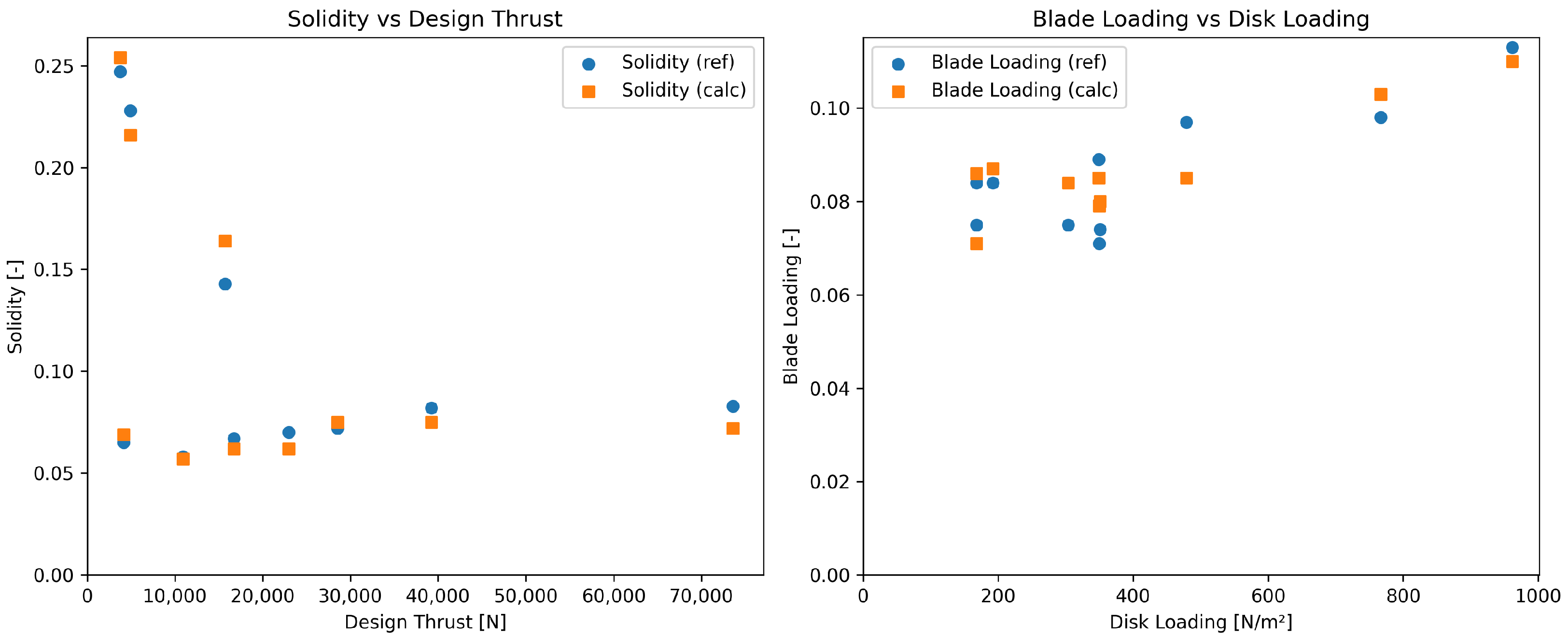
The dataset spans a wide design space in terms of size, thrust, and power, with rotor diameters between 2.23 and 16.36 m, hover thrust ranging from 3.8 to 73.6 kN, and hover power from 54 to 1569 kW. Disk loading varies substantially across configurations: conventional helicopters operate in a narrow range of 304–351 N/m², the NASA rotorcraft ranges from 168 to 192 N/m², while the powered-lift distributed propulsion concepts are significantly higher, ranging from 479 to 962 N/m². Regarding rotational speeds in hover, the helicopter designs operate at hover tip Mach numbers around 0.65, while the NASA concepts are designed with hover tip Mach numbers around 0.5, due to the design criterion of a reduced noise footprint. The solidity of the rotorcraft lies in the range of 0.058 to 0.083, while it is substantially higher for the powered-lift configurations, between 0.143 and 0.247, due to the higher disk loading. The blade loading for all configurations ranges from 0.071 to 0.113.

• Solidity prediction

The first part of the verification is to obtain the solidity based on rotor diameter, design thrust, rotational speed, and the advance ratio for each of the rotors in the dataset. One important note is that the blade stall initiation speed for each rotorcraft is assumed to be 5% above the cruise speed given in Table 2. Thus, the ${\mu }_{stall}$ values for the rotorcraft lie between 0.3 and 0.4. For the powered-lift configurations, the propellers must be able to carry the total weight during transition up to a certain speed. For all configurations, this forward velocity is assumed to be 35 m/s, corresponding to the point at which the tilt angle for the tiltwing configuration reaches 45 degrees (value from [19,29]). This results in a blade stall initiation advance ratio ${\mu }_{stall}$ of around 0.21.

The results for the solidity and corresponding blade loading are shown in

Table 3. Comparison of predicted and reference rotor parameters, including solidity, blade loading, hover power, and power loading, with relative deviations and MAPE values.

Parameter	Unit	Bo 105	EC 135	SA 365N	UH-60A	SMR TS	Quad TS	SbS E	TW TE	TR E	TR6 E	MAPE
Solidity	–	0.062	0.075	0.075	0.072	0.062	0.069	0.057	0.254	0.164	0.216
$\Delta$	%	−11.4	4.2	−8.5	−13.3	−6.9	6.2	−1.7	2.8	14.7	−5.3	7.5
Blade loading	–	0.084	0.085	0.080	0.079	0.087	0.071	0.086	0.110	0.085	0.103
$\Delta$	%	12.9	−4.1	9.3	11.6	4.6	−5.9	2.1	−2.6	−12.9	5.4	7.14
Hover power	kW	365	476	664	1314	222	54	137	115	325	126
$\Delta$	%	−7.6	−0.6	−10.6	−16.3	−16.8	−0.8	−5.4	10.2	−8.5	3.3	8.0
Power loading	kg/kW	6.3	6.1	6.0	5.6	7.6	8.0	8.1	3.4	4.9	4.0
$\Delta$	%	6.8	1.1	10.7	17.9	18.1	2.7	5.7	−8.4	9.2	−3.2	8.38

. On the left subplot of Figure 10, the solidity as a function of the design thrust is shown, while the normalized characteristic parameter, the blade loading as a function of disk loading, is presented on the right subplot of Figure 10. The comparison of calculated and reference solidity values shows overall good agreement across the full range of investigated rotors. As illustrated in Figure 10 (right), the model captures the general trend of increasing blade loading with increasing disk loading. The mean absolute percentage error (MAPE)mape amounts to 7.5%. The model tends to underpredict the solidity for the majority of the helicopter rotors, with differences ranging from $-1.7\%$ to $-13.3\%$. For the NASA UAM distributed propulsion configurations, the method tends to overpredict the solidity.

• Power calculation

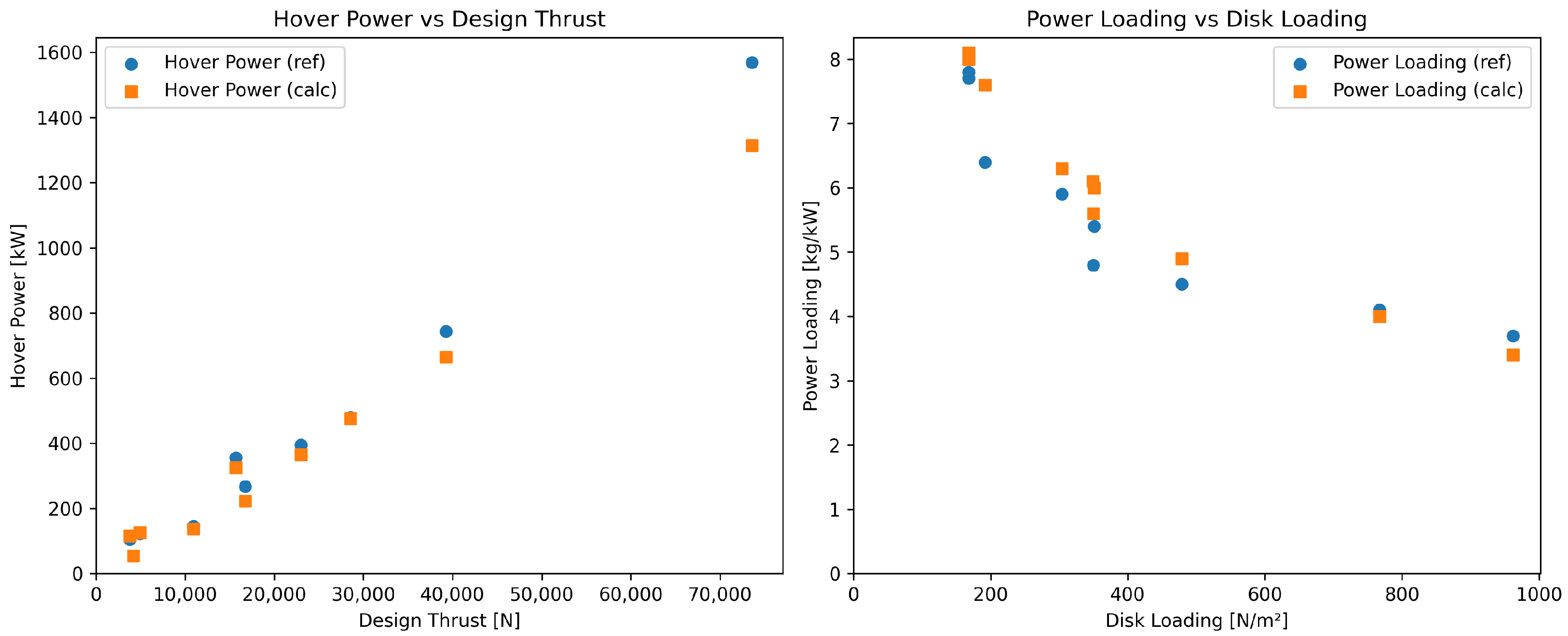
After sizing the investigated propellers, their performance in hover was calculated, with the results shown in Table 3. As shown in Figure 11 (left), the model accurately captures the expected increase in hover power with design thrust across the full range of configurations. Figure 11 (right) shows that the model also reproduces the inverse relationship between power loading and disk loading, with higher disk loading configurations exhibiting lower power loading due to increased induced power requirements. Similar to the solidity sizing, the calculated hover power agrees well with the reference data, with a mean absolute percentage error of 8.0%, indicating that the scaling of induced and profile power is well represented. The model tends to underpredict the hover power for the helicopter rotors, with deviations ranging from $-0.6\%$ to $-16.3\%$, while for the highly loaded powered-lift propellers of configurations TR6 E and TW TE, it overpredicts the power by 3.3% and 10.2%, respectively.

3.2. Battery Performance

Due to the characteristic eVTOL mission profile, the battery is subjected to high discharge currents both at the beginning and at the end of the mission. In particular, the landing segment requires the delivery of high power at an already low state of charge. As this represents a critical operating condition, it is essential to verify that the battery model accurately captures the discharge behavior over the entire depth of discharge, ensuring that the battery can be reliably sized with respect to both power and energy capacity.

• Description of the study case

For the verification of the battery discharge model, a representative experimental dataset from [60,61] was used. In that study, a comprehensive set of battery discharge profiles for eVTOL applications was generated based on experimental testing of lithium-ion cells under varied loading conditions. The dataset comprises measurements from 22 individual cells and captures the transient response of the battery under varying discharge rates.

The experiments were conducted using Sony-Murata 18650 VTC-6 cells [44], which are well suited for eVTOL applications due to their high specific energy and power capability. Each cell has a nominal capacity of 3200 mAh and a nominal voltage of 3.6 V, corresponding to a specific energy of approximately 230 Wh/kg. The cells are capable of sustaining continuous discharge C-rates of up to 10 C.

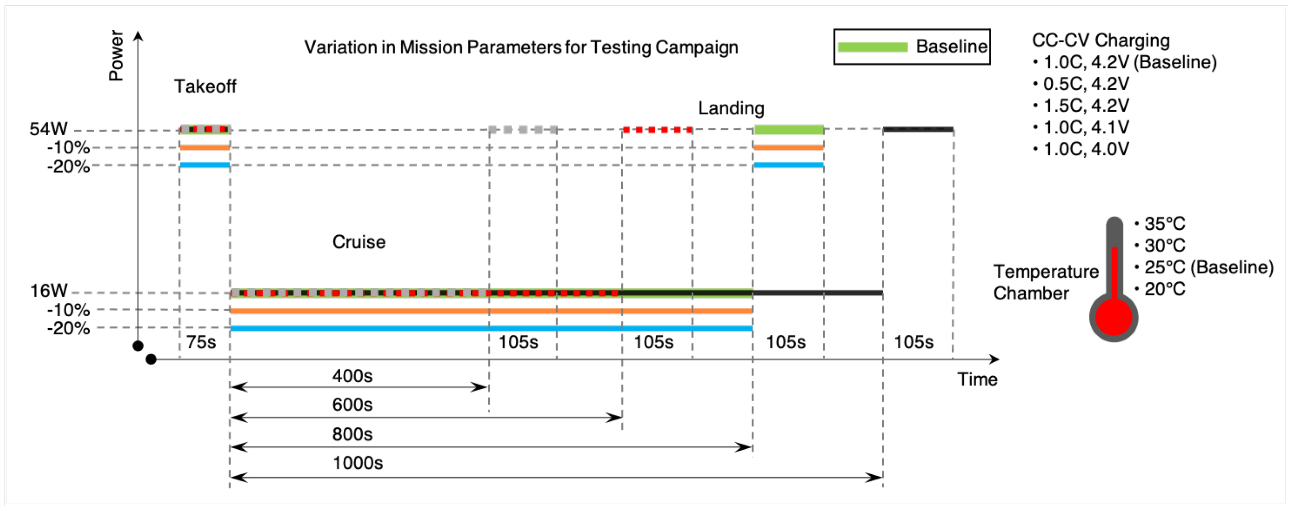
The representative mission profile for each of the experimental cases consists of three distinct phases: take-off, cruise, and landing, as illustrated in Figure 12. For the present verification, the most demanding test case was selected (VAH02 in [60], corresponding to the black line in Figure 12), which is characterized by an extended cruise duration and therefore results in a high depth of discharge prior to landing. The power profile is defined as follows:

• Take-off: 54 W for 75 s;
• Cruise: 16 W for 1000 s (increased from a baseline of 800 s);
• Landing: 54 W for 105 s.

• Discharge simulation results

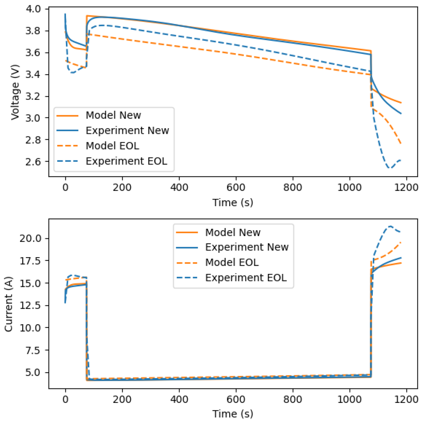
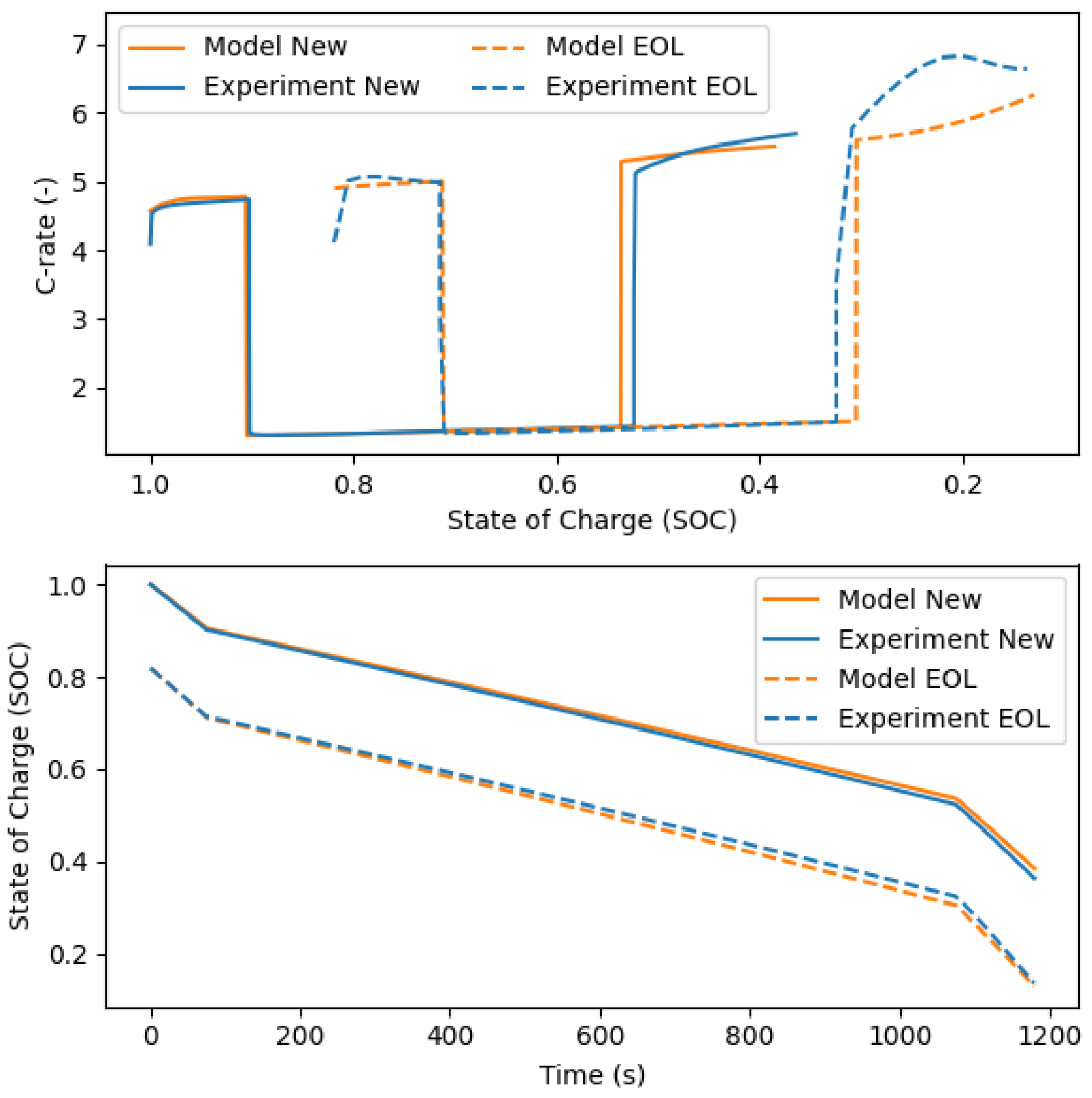
Since the battery discharge model does not include degradation effects, the verification mission was tested for two battery conditions: a new cell and a cell at the end of life (EOL). Key parameters such as the C-rate and state of charge (SOC) are shown in Figure 13, while the voltage and current profiles are presented in Figure 14.

In the upper subplot of Figure 13, the C-rate during discharge is illustrated. The new battery starts at an SOC of approximately 100%, while the end-of-life battery begins around 80%. As degradation effects are not explicitly included in the model, the 80% initial SOC is used as a proxy for the end-of-life battery with 80% state of health (SOH). Since the model does not include transient effects, sudden changes in power demand appear as sharp jumps. Overall, the C-rate predicted by the model follows the experimental values closely. The most critical region occurs when the SOC is low, and a large power demand is required—corresponding to the high-power burst during landing at the end of the mission. Here, the model cannot fully capture the strong nonlinearities, with a maximum deviation in instantaneous current/C-rate of approximately 15%. Although the model slightly underpredicts the instantaneous current during the landing power burst, this occurs over a short time interval and therefore has a negligible impact on the total discharged energy. Furthermore, the predicted C-rate remains well below the cell’s rated discharge limit and therefore does not affect the power requirements during landing.

For conceptual design and battery sizing, the total available energy and the corresponding depth of discharge are of major importance. This is shown in the lower subplot of Figure 13, where the SOC decrease closely follows the experimental data for both new and end-of-life cells. For the new cell, the SOC decreases from 100% to about 36% (experiment) versus 38% (model), corresponding to roughly a 5% deviation. For the end-of-life cell, SOC decreases from 82% to 13% with a deviation of less than 1%.

3.3. Vehicle Sizing Verification

To verify the overall sizing procedure, two eVTOL aircraft are designed based on the NASA UAM reference mission defined in [8]. The reference vehicles were designed using NDARC [14], where CAMRAD II [62] was employed for the rotor aerodynamic design. The corresponding vehicle geometries were generated using the CAD OpenVSP [63].

The reference vehicles are publicly available online [29]. The dataset includes OpenVSP models, from which the geometric data used in this comparison are extracted, as well as NDARC input files that enable verification of modeling assumptions, particularly with respect to mass estimation.

3.3.1. Vehicle and Mission Description

• Mission description

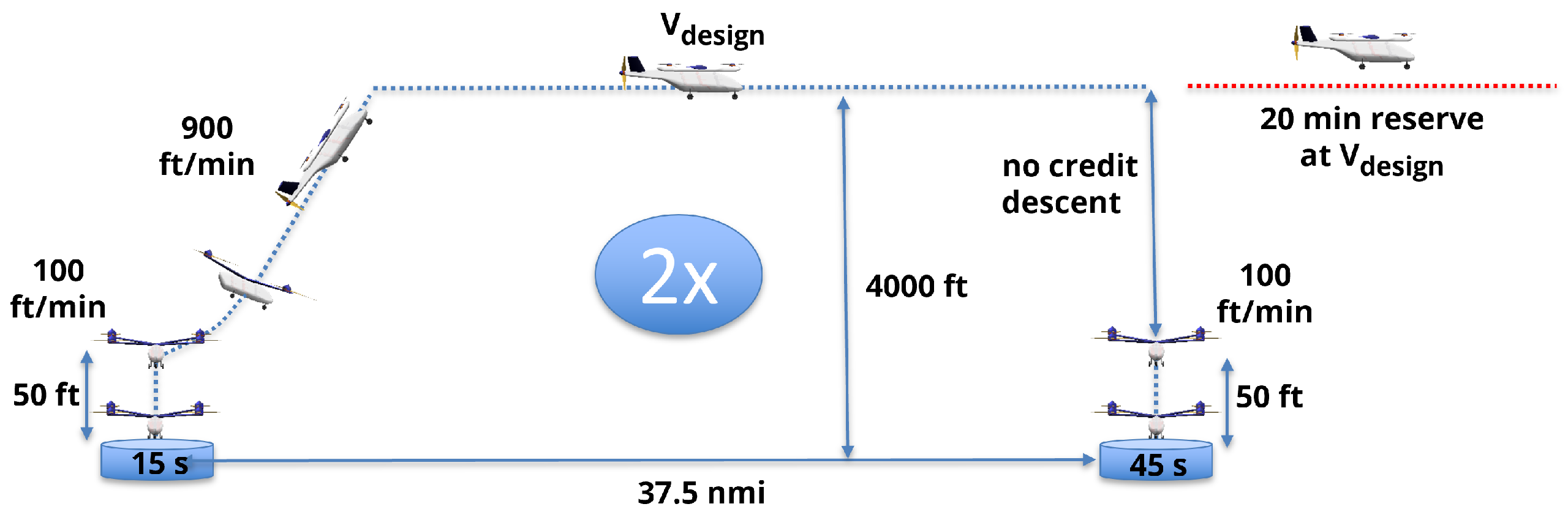
A summary of the primary design mission segments is provided in

Table 4. Parameters of the individual mission segments of the implemented verification mission. Adapted from [8].

Segment	1	2	3	4	5	6	7	8
Initial Alt. (MSL ISA) [ft]	6000	6000	6050	6500	10,000	6050	6000	10,000
Final Alt. (MSL ISA) [ft]	6000	6050	6500	10,000	10,000	6000	6000	10,000
Time [s]	15	30	$t_{\mathrm{climb},\mathrm{tr}}$	$t_{\mathrm{climb}}$	$t_{\mathrm{cruise}}$	30	45	1200
Distance [nmi]	–	0	$D_{\mathrm{climb},\mathrm{tr}}$	$D_{\mathrm{climb}}$	$37.5-D_{\mathrm{climb}}$	0	0	$D_{\mathrm{cruise},\mathrm{res}}$
Speed [knots]	–	–	$V_{\mathrm{y}}$	$V_{\mathrm{y}}$	$V_{\mathrm{br}}$	0	0	$V_{\mathrm{br}}$
ROC [ft/min]	–	100	900	900	0	$-100$	0	0
Percent of Max Power	100%	100%	100%	$P_{\mathrm{climb}}$	$P_{\mathrm{cruise}}$	100%	100%	$P_{\mathrm{cruise}}$

, and the corresponding mission profile is illustrated in Figure 15. The mission consists of two legs, each with a range of 37.5 nmi (≈70 km), and includes a reserve of 20 min at cruise power. The operations assume a take-off and landing altitude of 6000 ft (≈1830 m) and a cruise altitude of 10,000 ft (≈3000 m).

The implemented mission profile differs slightly from the original NASA definition in order to align with the capabilities of the present tool. In the reference mission, take-off and landing are modeled as taxi segments at 10% power for 15 s, and the landing transition is assumed to last 30 s. In the present work, these phases are approximated by a 15 s hover during take-off and a total of 45 s hover during landing.

Furthermore, the transition climb in the NASA mission is modeled as a 10 s segment at 100% power. In contrast, the current implementation assumes a linear acceleration phase. For the multirotor configuration, a climb rate of 900 ft/min is used. For the powered-lift configuration, the transition consists of a climb to 500 ft, followed by a fixed-wing climb to 4000 ft above ground level.

Another characteristic of the mission profile, consistent with the NASA UAM reference mission, is that no explicit descent segment is defined. Instead, the cruise segment is maintained until the landing phase begins. This approach leads to a conservative estimate of energy consumption, since the potential energy associated with altitude loss is not recovered through a dedicated descent segment.

• Vehicle Description

For the vehicles, the design payload requirement is defined as 1200 lb (approximately 540 kg), corresponding to six passengers, each with a mass of 90 kg and 10 kg of luggage. The battery technology is assumed to have a pack-level effective gravimetric energy density of 400 Wh/kg, of which 30% accounts for battery management systems and pack structural components. The battery depth of discharge is 80%, corresponding to a discharge from 95% to 15% state of charge.

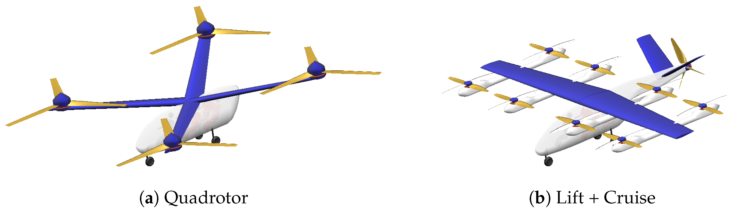
Two representative eVTOL configurations are considered for the verification of the sizing methodology, as shown in Figure 16.

The first configuration is a Quadrotor design. This vehicle utilizes four three-bladed lift-propellers, analogous to helicopter rotors, which provide vertical lift during hover and both lift and propulsive thrust during forward flight. The rotors are arranged in an X-configuration (tandem pair arrangement). The rotor tip speed is set to 500 ft/s (approximately 168 m/s), corresponding to a tip Mach number of 0.5, which is selected to satisfy noise constraints. The overall landing footprint is approximately 20 m, resulting in a rotor diameter of about 8 m.

The second configuration is a Lift + Cruise design. This vehicle employs eight lift-propellers distributed laterally along the wing, both forward and aft, to provide vertical lift during hover and low-speed flight. In addition, a single pusher propeller is used to generate thrust during cruise. The lift-propellers operate at the same tip speed as the Quadrotor configuration to satisfy equivalent noise constraints, with a rotor diameter of approximately 3 m. A two-bladed rotor design is assumed. The wing is optimized for cruise performance, as low-speed flight is supported by lift augmentation from the distributed lift-propellers. This enables efficient fixed-wing operation during the cruise segment while maintaining vertical take-off and landing capability.

3.3.2. Results

The overall dimensions and performance parameters of the vehicles sized using the present methodology are compared with the NASA reference data in

Table 5. Comparison of vehicle parameters between NASA reference and present configurations.

Parameter	Unit	Quad Ref	Quad	L + C Ref	L + C	$\mathsf{\Delta }$ Quad [%]	$\mathsf{\Delta }$ L + C [%]
Number lifters	-	4	4	8	8	-	-
Number pusher	-	0	0	1	1	-	-
Hover thrust/lifter	N	7208	7252	4566	4712	0.6	3.2
Lifter disk loading	N/m2	143.7	146.7	627.4	641.6	2.1	2.3
Lifter radius	m	3.99	3.97	1.52	1.53	−0.6	0.3
Solidity	-	0.055	0.060	0.267	0.198	8.5	−25.7
Hover tip speed	m/s	168	167	178	167	−0.6	−6.6
Wing span	m	-	-	15.24	15.00	-	−1.57
Wing area	m2	-	-	19.54	18.94	-	−3.05
Wing MAC	m	-	-	1.03	1.3	-	26.19
Wing aspect ratio	-	-	-	12.13	11.88	-	−2.06
Fuselage length	m	6.40	5.44	9.14	10.47	−15.0	14.5
Fuselage height	m	2.02	1.54	1.87	1.54	−23.8	−17.4
Fuselage width	m	1.91	1.52	1.76	1.52	−20.2	−13.4
Hover power	kW	345	381	827	932	10.3	12.6
Cruise power	kW	263	268	246	273	2.1	10.9
Battery capacity	kWh	370	379	399	454	2.6	13.7
Cruise speed	km/h	181	180	207	210	−0.8	1.2
Effective L/D (WV/P)	-	5.8	5.4	8.5	8.1	−6.7	−5.1
Hover FM	-	0.7	0.7	0.74	0.76	0	2.7
Hover C-rate	1/h	1.1	1.0	2.4	2.2	−13.6	−8.8
Cruise C-rate	1/h	0.8	0.7	0.7	0.7	−10.0	−4.3

. In this study, the focus is placed on the comparison of mass properties, mission performance characteristics, and battery sizing.

• Mass estimation

The maximum take-off mass is a key design parameter, as it directly affects aircraft performance, structural requirements, and energy efficiency. An analysis of the mass distribution across different eVTOL configurations enables the identification of dominant contributors and potential areas for improving overall cost-effectiveness.

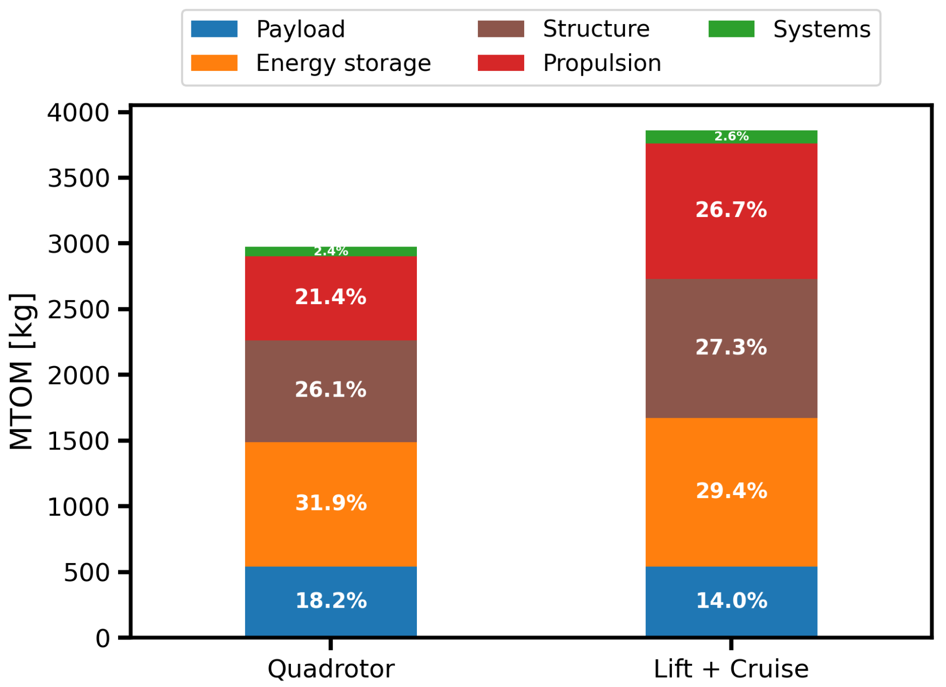
Figure 17 illustrates the mass distributions of the Quadrotor and Lift + Cruise configurations according to the breakdown defined in Section 2.6. The MTOM of the Quadrotor is 2957 kg, whereas the Lift + Cruise configuration is approximately 30% heavier, with a MTOM of 3843 kg.

Energy storage represents the largest mass fraction in both configurations, accounting for approximately 32% of the MTOM for the Quadrotor and 30% for the Lift + Cruise vehicle. The structural mass is the second largest contributor, representing slightly more than one quarter of the total mass in both cases.

A significant difference is observed in the propulsion system mass. For the Lift + Cruise configuration, the propulsion mass is comparable to the structural mass, whereas the Quadrotor exhibits a substantially lower propulsion mass fraction. This difference can be attributed to two main factors. First, the Quadrotor is not sized for an OEI condition. Second, the larger rotors of the Quadrotor result in lower disk loading in hover and consequently higher power loading compared to the Lift + Cruise configuration, leading to a lower required total motor mass.

As a result, the useful payload fraction of the Quadrotor corresponds to approximately 18% of the MTOM, compared to a lower value of about 14% for the Lift + Cruise configuration.

• Mass breakdown comparison

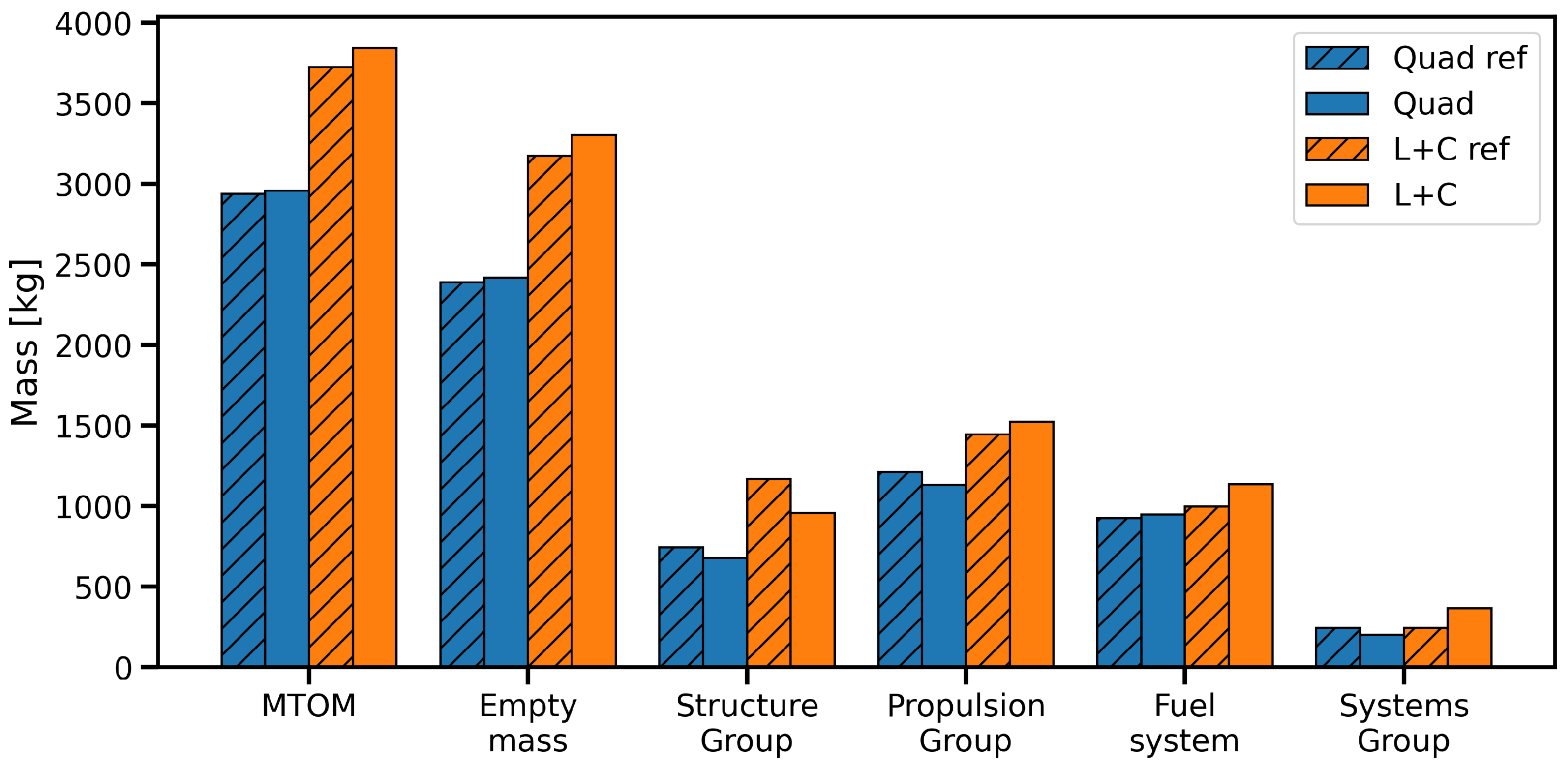
For comparison with NASA UAM reference vehicles [29], the component masses are reformulated to align as closely as possible with the NDARC mass group definitions. The resulting comparison is presented in Figure 18 and

Table 6. Quantitative comparison of mass breakdown with NASA UAM reference vehicles using NDARC mass group definitions.

Mass Parameter [kg]	Quad Ref	Quad	L + C Ref	L + C	$\mathsf{\Delta }$Quad [%]	$\mathsf{\Delta }$L + C [%]
MTOM	2939	2957	3724	3843	0.6	3.2
Empty mass	2390	2417	3176	3303	1.1	4.0
Structure Group	744	677	1168	956	−9.0	−18.1
Propulsion Group	1212	1131	1445	1523	−6.6	5.4
Fuel system	924	949	998	1134	2.6	13.6
Systems Group	243	202	245	364	−17.0	48.4

.

Overall, both configurations reproduce the NDARC reference masses well at the top level, particularly in terms of maximum take-off mass and empty mass. The agreement is generally good, with only minor deviations that can largely be attributed to differences in modeling approaches. For the Quadrotor, the converged MTOM is approximately 18 kg (0.6%) higher than the reference, while for the Lift + Cruise configuration the deviation is 79 kg (3.2%). The empty mass deviations are of similar magnitude, with increases of 1.1% for the Quadrotor and 4.0% for the Lift + Cruise configuration.

More pronounced differences are observed at the subsystem level. In particular, the structural mass is consistently underpredicted. The structure group is approximately 9% lighter for the Quadrotor and 18.1% lighter for the Lift + Cruise configuration, indicating a comparatively simplified structural modeling approach. For example, the NASA reference vehicle assumes a propeller pylon mass of approximately 35 lb (15 kg) per pylon, with an additional 20 lb allocated for the forward propeller (available in the supplementary material for [18] via [29]). In contrast, the model described in Section Pylons predicts pylon masses that are roughly 50% lower. This structural mass difference is also influenced by the fact that the forward propeller pylon is not modeled.

The propulsion group shows differences of approximately 100 kg for both configurations. The Quadrotor propulsion mass is underpredicted by 6.6%, whereas the Lift + Cruise configuration shows a 5.4% higher propulsion mass compared to NDARC. Since the same underlying propulsion sizing relations are used (see Section 2.6.3), these deviations are primarily attributed to differences in design conditions and the resulting power requirements.

The fuel system group, representing the battery in this study, reflects differences in required mission energy. For the Quadrotor, the battery capacity is 2.6% higher than the reference, while for the Lift + Cruise configuration the deviation increases to 13.6%. These differences are consistent with the higher power requirements predicted by the present model (see Table 5). In particular, the Quadrotor exhibits increased hover power by 10.3% and cruise power by 2.6%, whereas the Lift + Cruise configuration shows 12.6% higher power requirements in hover and 10.9% in cruise, leading to a larger increase in required battery mass. For the Lift + Cruise configuration, the discrepancy in cruise power is likely the result of the combined effects of the higher gross weight of the sized vehicle, differences in the pusher propeller design and associated propulsive efficiency, and deviations in the aerodynamic drag prediction compared with the NDARC reference model.

The largest discrepancy is observed in the systems group, which is strongly influenced by differences in modeling assumptions. For the Quadrotor, the NASA reference vehicle includes a gearbox system connecting the four rotors, which is not modeled in the present framework. This results in a systems mass that is approximately 17% lower in the current model. Additionally, the treatment of the power electronics system differs, as this is explicitly included in the systems group in the present work. Thus, for the Lift + Cruise configuration, the discrepancy is therefore more pronounced, with the systems mass 48.4% higher than the NASA reference. This is primarily due to the use of a flight control weight estimation method derived from FLOPS [53], which predicts significantly higher fixed-wing flight control masses compared to the NDARC [14] model.

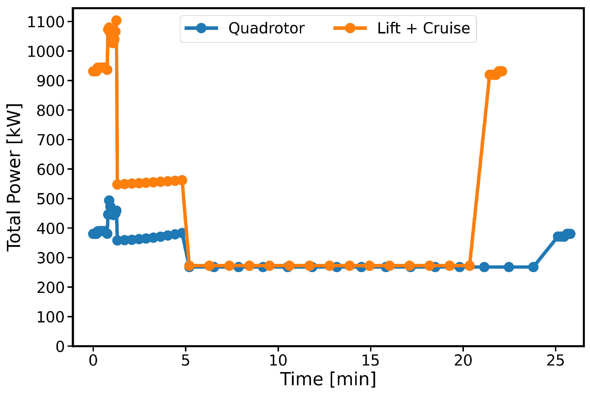
• Power consumption profile

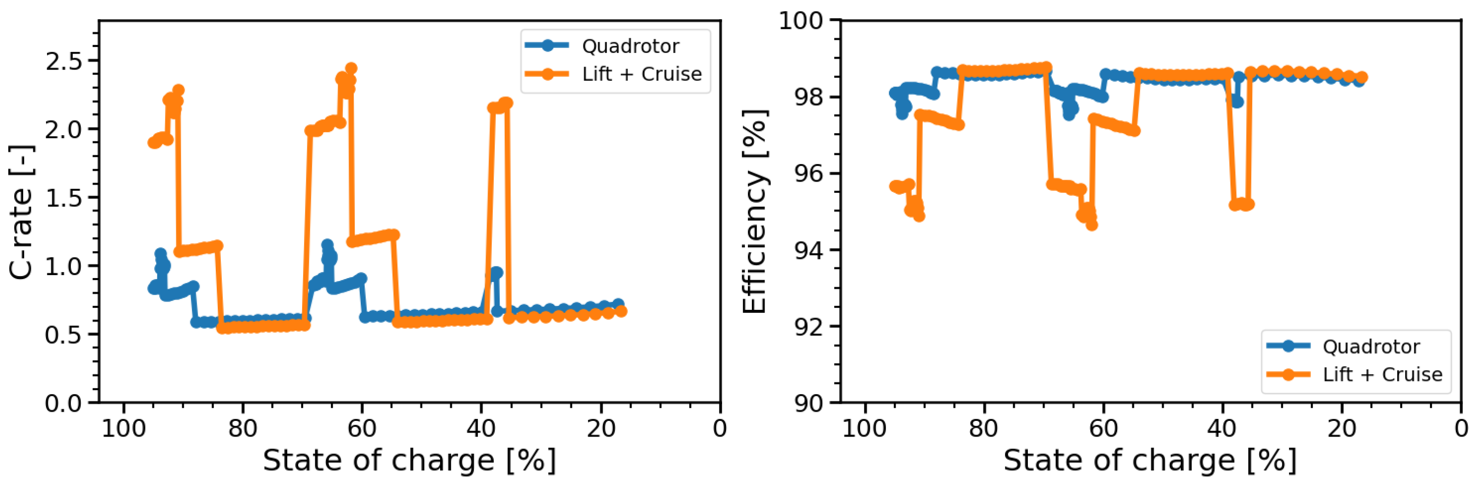
The next part of the analysis focuses on the performance of the vehicles throughout the design mission. Figure 19 presents the total power consumption along the mission profile. The values correspond to propeller shaft power, including constant losses of 5% for the electric motors and 2% for the power electronics.

Significant peaks in power demand occur during the hover and initial climb segments. The Quadrotor requires approximately 381 kW in hover, whereas the Lift + Cruise configuration reaches about 931 kW. This substantial difference is consistent with the approximately 30% higher MTOM of the Lift + Cruise vehicle and its significantly higher disk loading (by a factor of about 4.3), which directly increases the induced power required to generate lift in hover.

During the axial climb phase, both configurations exhibit only a modest increase in power relative to hover, with a maximum increment of approximately 10 kW.

At the beginning of the transition segment, corresponding to rotorcraft climb for the Quadrotor and acceleration to wing-borne flight for the Lift + Cruise configuration, a pronounced increase in total power is observed. The required power rises by approximately 15%, reaching about 446 kW for the Quadrotor and 1.07 MW for the Lift + Cruise vehicle. This increase is primarily attributed to the additional propulsive power required to accelerate the aircraft to cruise speed. Since a constant acceleration during transition climb is assumed, its impact is most significant at low forward velocities. In the second climb segment above 500 ft, both vehicles exhibit a reduction in power demand, with values of approximately 383 kW for the Quadrotor and 562 kW for the Lift + Cruise configuration at the top of climb.

Despite the Lift + Cruise vehicle being considerably heavier, both configurations exhibit similar cruise power levels. This can be explained by differences in aerodynamic efficiency. The ratio of cruise-to-hover power is approximately 0.7 for the Quadrotor and only 0.3 for the Lift + Cruise configuration. This behavior is consistent with the effective lift-to-drag ratio, defined as $WV/P$. The Quadrotor achieves an effective lift-to-drag ratio of 5.4, whereas the Lift + Cruise configuration reaches 8.1, reflecting the superior aerodynamic efficiency of fixed-wing flight.

• Battery discharge

Another important aspect enabled by the inclusion of the battery model is the analysis of the C-rate variation throughout the mission, as shown in the left plot of Figure 20. The highest C-rates occur during the high-power vertical flight segments, namely hover and climb. In addition, as the battery state of charge decreases, the C-rate increases for the same power demand, as expected.

For the Lift + Cruise configuration, the C-rate during take-off hover in the first mission leg is approximately 1.9 at a high SOC of 95%. During the final landing after the second leg, when the SOC has decreased to about 35%, the C-rate increases to approximately 2.2 for the same power requirement. The maximum C-rate, around 2.5, is reached during the transition climb segment. In contrast, during cruise, the C-rate remains relatively low and stable, typically in the range of 0.6–0.7 throughout the mission.

For the Quadrotor configuration, the battery loading is more uniform across all mission segments. The maximum C-rate occurs during the climb, reaching approximately 1.2, while hover conditions correspond to values close to 1.0. During cruise, the C-rate is again in the range of 0.6–0.7, similar to the Lift + Cruise configuration.

As shown in Table 5, the predicted C-rate values are in good agreement with the NASA reference data, with deviations of approximately 10%.

The battery loading can also be interpreted in terms of efficiency losses, as illustrated in the right plot of Figure 20. The battery efficiency is defined as

$$\eta =1-{\displaystyle \frac{I R_{\mathrm{tot}}}{V_{\mathrm{OC}}}}$$

(55)

For the Quadrotor, the battery efficiency remains high, in the range of 98–99%, since both hover and cruise occur at C-rates close to one. In contrast, the Lift + Cruise configuration exhibits lower efficiency during high-power vertical flight segments, where it decreases to approximately 96%, while during cruise it remains around 98%. Furthermore, it can be observed that, for a given power demand, the battery efficiency decreases as the state of charge is reduced, reflecting the increased relative impact of internal resistance losses.

4. Conclusions

In this study, an integrated and iterative framework for the conceptual design and sizing of eVTOL aircraft is presented. While based on a low-fidelity design philosophy, the methodology provides a structured and physically consistent approach. Starting from a limited set of inputs—top-level requirements, operational constraints, and technology assumptions—the process iteratively combines component sizing, mission analysis, battery sizing, and mass estimation until convergence in key parameters such as maximum take-off mass and battery capacity is achieved.

To evaluate the methodology, selected key methods extending beyond standard handbook approaches were verified. First, the solidity sizing and hover performance of lifting propellers were compared against a dataset of conventional helicopter rotors and powered-lift propellers covering a wide range of thrust and loading conditions. Good agreement was observed, with mean absolute percentage errors of 7.5% for solidity and 8.0% for hover power. Second, the battery discharge model was verified against experimental data for the Sony-Murata 18650 VTC-6 cell under an eVTOL-representative mission profile. The model accurately captures both C-rate and state-of-charge evolution. The predicted depth of discharge shows good agreement with experiments, with deviations of about 5% for a new cell and less than 1% for an end-of-life cell.

Finally, the overall aircraft sizing has been evaluated for two representative configurations, a wingless Quadrotor and a powered-lift Lift + Cruise, by comparison with results obtained using the state-of-the-art rotorcraft design tool NDARC. The sizing is based on a two-leg 70 km mission with a 20-min reserve, transporting six occupants and assuming a battery gravimetric energy density of 400 Wh/kg. Overall, good agreement with the reference data is achieved. The maximum take-off mass deviates by 0.6% for the Quadrotor and 3.2% for the Lift + Cruise configuration, with similar trends for the empty mass (1.1% and 4.0%). Differences in battery sizing reflect variations in predicted mission energy demand. The Quadrotor shows a 2.6% higher battery capacity, while the Lift + Cruise deviation reaches 13.6%, driven by higher predicted power requirements, especially in hover and cruise, which lead to an increased battery mass. The predicted C-rate behavior is also consistent with the reference data. For the Lift + Cruise configuration, the hover C-rate is about 2.2 during final landing compared to 2.4 in the NASA reference, while cruise remains low at around 0.6 versus 0.7. The Quadrotor shows a more uniform loading, with C-rates around 1.0 in hover and similarly low values in cruise. Overall, the C-rate predictions agree well with the NASA data, with deviations on the order of 10%.

Beyond numerical agreement, the results highlight the main design couplings in eVTOL sizing. The link between propeller sizing, disk loading, and power demand makes the dominant design drivers explicit: the higher hover power of the Lift + Cruise configuration is directly tied to its increased disk loading and MTOM, illustrating the strong coupling between propulsion and overall mass. The battery model further enables a realistic assessment of mission feasibility, particularly under high-power, low-SOC conditions during landing.

Overall, the results emphasize that both power and energy must be considered simultaneously. While Lift + Cruise benefits from better cruise efficiency, this is partly offset by higher vertical-flight power demand, which drives battery and system mass. As a result, trade-offs between disk loading, aerodynamic efficiency, and propulsion architecture become central early-stage design decisions, which the framework can systematically support.

At the same time, several limitations of the current methodology have been identified. The propeller model, while capturing overall trends, shows systematic deviations, particularly an underprediction of rotor solidity and hover power at low disk loading, and an overprediction for highly loaded distributed propulsion systems. These discrepancies are primarily attributed to aerodynamic effects that are not explicitly resolved in the present formulation. In particular, detailed blade geometry effects, tip losses, and non-uniform inflow distributions are only implicitly accounted for, while the induced power factor remains a key tuning parameter that requires further refinement to improve predictive accuracy across the full operating envelope. In addition, the regression-based component mass estimation introduces sensitivity to the assumed technology factors. While this approach enables rapid assessment in early design stages, it inherently depends on calibration against existing or projected datasets, and therefore requires periodic updating to remain representative of future technological advancements.

Future research directions can be grouped into three main areas.

The first area focuses on improving uncertainty treatment and the robustness of the sizing methodology itself. A key aspect is the treatment of aerodynamic and powertrain-related uncertainties, in particular the refinement of the induced power factor within the propeller model. The component mass estimation approach could further be strengthened by updating regression models where necessary or progressively replacing them with physics-based formulations to reduce reliance on technology factors. This would also enable the extension of the framework to additional propulsion concepts such as ducted fans, as well as alternative powertrains, including hybrid-electric architectures based on carbon fuels or hydrogen. In addition, the electrical power system sizing could be expanded to incorporate redundancy and failure modes, such as inverter or battery module failures, enabling more resilient and realistic design assessments.

The second research direction concerns the extension toward multi-mission and system-level optimization. Instead of relying on a single design mission, future work could evaluate a broader set of operational scenarios with varying payload, range, and utilization patterns. This would enable the derivation of more robust and globally optimal aircraft configurations that account not only for performance, but also for economic metrics, environmental impact, and anticipated passenger demand.

The third area addresses operational integration and real-world deployment aspects. This includes the modeling of ground infrastructure requirements such as vertiport layout, helipad sizing, and turnaround procedures. In this context, different concepts of operation (ConOps) could be analyzed, including scenarios involving partial or no recharging between consecutive missions. Such considerations are essential to bridge the gap between conceptual vehicle design and feasible urban air mobility system implementation.

References

1. Tiede, B.; O’Meara, C.; Jansen, R. Battery Key Performance Projections based on Historical Trends and Chemistries. In Proceedings of the 2022 IEEE Transportation Electrification Conference & Expo (ITEC), Anaheim, CA, USA, 15–17 June 2022; pp. 754–759. [Google Scholar] [CrossRef]
2. Deepak, K.; Frikha, M.A.; Benômar, Y.; El Baghdadi, M.; Hegazy, O. In-Wheel Motor Drive Systems for Electric Vehicles: State of the Art, Challenges, and Future Trends. Energies 2023, 16, 3121. [Google Scholar] [CrossRef]
3. Xia, J.; Zhou, Z. The Modeling and Control of a Distributed-Vector-Propulsion UAV with Aero-Propulsion Coupling Effect. Aerospace 2024, 11, 284. [Google Scholar] [CrossRef]
4. Reiche, C.; Goyal, R.; Cohen, A.; Serrao, J.; Kimmel, S.; Fernando, C.; Shaheen, S. Urban Air Mobility Market Study; Technical Report; National Aeronautics and Space Administration (NASA): Washington, DC, USA, 2018. [Google Scholar]
5. Michelmann, J.; Straubinger, A.; Becker, A.; Al Haddad, C.; Plötner, K.O.; Hornung, M. Urban air mobility 2030+: Pathways for UAM-a scenario-based analysis. In Proceedings of the Deutscher Luft- und Raumfahrtkongress (German Aerospace Congress); DGLR: Bonn, Germany, 2020. [Google Scholar]
6. Goyal, R.; Reiche, C.; Fernando, C.; Cohen, A. Advanced Air Mobility: Demand Analysis and Market Potential of the Airport Shuttle and Air Taxi Markets. Sustainability 2021, 13, 7421. [Google Scholar] [CrossRef]
7. Asmer, L.; Pak, H.; Prakasha, P.S.; Schuchardt, B.I.; Weiand, P.; Meller, F.; Torens, C.; Becker, D.; Zhu, C.; Schweiger, K.; et al. Urban Air Mobility Use Cases, Missions and Technology Scenarios for the HorizonUAM Project. In Proceedings of the AIAA Aviation 2021 Forum, Virtual Event, 2–6 August 2021. [Google Scholar] [CrossRef]
8. NASA Langley Research Center; Patterson, M.; Antcliff, K.; Kohlman, L. A Proposed Approach to Studying Urban Air Mobility Missions Including an Initial Exploration of Mission Requirements. In Proceedings of the Vertical Flight Society 74th Annual Forum, Phoenix, AZ, USA, 14 May 2018; pp. 1–19. [Google Scholar] [CrossRef]
9. Doo, J.T.; Pavel, M.D.; Didey, A.; Hange, C.; Diller, N.P.; Tsairides, M.A.; Smith, M.; Bennet, E.; Bromfield, M.; Mooberry, J. NASA Electric Vertical Takeoff and Landing (eVTOL) Aircraft Technology for Public Services—A White Paper; NASA Transformative Vertical Flight Working Group 4; Technical Report; NASA: Washington, DC, USA, 2021. [Google Scholar]
10. Alsalem, A.; Zohdy, M. A Review on Civil Applications of Vertical Take-Off and Landing Vehicles. In Proceedings of the 2023 IEEE Conference on Technologies for Sustainability (SusTech), Portland, OR, USA, 19–22 April 2023; pp. 130–137. [Google Scholar] [CrossRef]
11. Goyal, R.; Cohen, A. Advanced Air Mobility: Opportunities and Challenges Deploying eVTOLs for Air Ambulance Service. Appl. Sci. 2022, 12, 1183. [Google Scholar] [CrossRef]
12. Chappelle, C.; Li, C.; Vascik, P.D.; Hansman, R.J. Opportunities to Enhance Air Emergency Medical Service Scale through New Vehicles and Operations. In Proceedings of the 2018 Aviation Technology, Integration, and Operations Conference; American Institute of Aeronautics and Astronautics: Reston, VA, USA, 2018. [Google Scholar] [CrossRef]
13. Bruder, F.; Erd, A.; Benk, D.; Brütsch, L.; Zöllinger, F.; Schwierz, M.; Houzenga, E.; Himmelreich, P.; Maximilian, K.H.; Blume, H.; et al. Multicopter in the Rescue Service: Feasibility Study on the Application Potential of Multicopters as Emergency Doctor Shuttles; Technical Report; ADAC Luftrettung: Munich, Germany, 2020. [Google Scholar] [CrossRef]
14. Johnson, W.; Field, M. NASA Design and Analysis of Rotorcraft; Technical Report NASA/TP–20220000355/Vol 1; NASA: Washington, DC, USA, 2022. [Google Scholar]
15. Weiand, P.; Buchwald, M.; Schwinn, D. Process Development for Integrated and Distributed Rotorcraft Design. Aerospace 2019, 6, 23. [Google Scholar] [CrossRef]
16. Basset, P.M.; Beaumier, P.; Rakotomamonjy, T. CREATION: A numerical workshop for rotorcraft concepts generation and evaluation. In Proceedings of the Rotorcraft Virtual Engineering Conference, Liverpool, UK, 8–10 November 2016. [Google Scholar]
17. Lukaczyk, T.W.; Wendorff, A.D.; Colonno, M.; Economon, T.D.; Alonso, J.J.; Orra, T.H.; Ilario, C. SUAVE: An Open-Source Environment for Multi-Fidelity Conceptual Vehicle Design. In Proceedings of the 16th AIAA/ISSMO Multidisciplinary Analysis and Optimization Conference, Dallas, TX, USA, 22–26 June 2015. [Google Scholar] [CrossRef]
18. Silva, C.; Johnson, W.R.; Solis, E.; Patterson, M.D.; Antcliff, K.R. VTOL Urban Air Mobility Concept Vehicles for Technology Development. In Proceedings of the 2018 Aviation Technology, Integration, and Operations Conference, Atlanta, GA, USA, 25–29 June 2018. [Google Scholar] [CrossRef]
19. Whiteside, S.K.S.; Pollard, B.P.; Antcliff, K.R.; Zawodny, N.S.; Fei, X.; Silva, C.; Medina, G.L. Design of a Tiltwing Concept Vehicle for Urban Air Mobility; Technical Report NASA/TM–20210017971; NASA: Washington, DC, USA, 2021. [Google Scholar]
20. Whiteside, S.K.S.; Pollard, B.P. Conceptual Design of a Tiltduct Reference Vehicle for Urban Air Mobility. In Proceedings of the Aeromechanics for Advanced Vertical Flight Technical Meeting, Transformative Vertical Flight 2022, San Jose, CA, USA, 25–27 January 2022. [Google Scholar]
21. Radotich, M. Conceptual Design of Tiltrotor Aircraft for Urban Air Mobility. In Proceedings of the Aeromechanics for Advanced Vertical Flight Technical Meeting, Transformative Vertical Flight 2022, San Jose, CA, USA, 25–27 January 2022. [Google Scholar]
22. Atci, K.; Weiand, P.; Guner, F. Understanding the fixed pitch RPM-controlled rotor modeling for the conceptual design of UAM vehicles. CEAS Aeronaut. J. 2024, 15, 409–422. [Google Scholar] [CrossRef]
23. Basset, P.M.; Vu, B.D.; Beaumier, P.; Reboul, G.; Ortun, B. Models and Methods at ONERA for the Presizing of eVTOL Hybrid Aircraft Including Analysis of Failure Scenarios. In Proceedings of the 74th Annual Vertical Flight Society Forum and Technology Display 2018 (FORUM 74); The Vertical Flight Society: Fairfax, VA, USA, 2018. [Google Scholar]
24. Brown, A.; Harris, W. A Vehicle Design and Optimization Model for On-Demand Aviation. In Proceedings of the 2018 AIAA/ASCE/AHS/ASC Structures, Structural Dynamics, and Materials Conference, Kissimmee, FL, USA, 8–12 January 2018. [Google Scholar] [CrossRef]
25. Palaia, G.; Abu Salem, K.; Cipolla, V.; Binante, V.; Zanetti, D. A Conceptual Design Methodology for e-VTOL Aircraft for Urban Air Mobility. Appl. Sci. 2021, 11, 10815. [Google Scholar] [CrossRef]
26. Courtin, C.; Mahseredjian, A.; Dewald, A.J.; Drela, M.; Hansman, J. A Performance Comparison of eSTOL and eVTOL Aircraft. In AIAA AVIATION 2021 FORUM; AIAA AVIATION Forum; American Institute of Aeronautics and Astronautics: Reston, VA, USA, 2021. [Google Scholar] [CrossRef]
27. Ugwueze, O.; Statheros, T.; Horri, N.; Bromfield, M.A.; Simo, J. An Efficient and Robust Sizing Method for eVTOL Aircraft Configurations in Conceptual Design. Aerospace 2023, 10, 311. [Google Scholar] [CrossRef]
28. Yanev, R.Y.; Staack, I. Framework Development for Conceptual Design and Configuration Analysis of eVTOL Aircraft. In Proceedings of the 34th Congress of the International Council of the Aeronautical Sciences, ICAS 2024, Florence, Italy, 9–13 September 2024. [Google Scholar]
29. NASA Langley Research Center, Systems Analysis and Concepts Directorate. NASA UAM Reference Vehicles. Available online: https://www.nasa.gov/reference/uam-refs/ (accessed on 16 February 2026).
30. Gudmundsson, S. General Aviation Aircraft Design: Applied Methods and Procedures, 2nd ed.; Butterworth-Heinemann: Oxford, UK; Cambridge, MA, USA, 2022. [Google Scholar]
31. Johnson, W. Rotorcraft Aeromechanics; Number 36 in Cambridge Aerospace Series; Cambridge University Press: Cambridge, MA, USA, 2013. [Google Scholar]
32. Leishman, J.G. Principles of Helicopter Aerodynamics, 2nd ed.; Number 18 in Cambridge Aerospace Series; Cambridge University Press: Cambridge, MA, USA, 2006. [Google Scholar]
33. McCormick, B.W. Aerodynamics of V/STOL Flight; Dover Publications: Mineola, NY, USA, 1999. [Google Scholar]
34. Roskam, J. Airplane Design. 5: Component Weight Estimation, 3rd ed.; DARcorporation: Lawrence, KS, USA, 2003. [Google Scholar]
35. Williams, J.E.; Vukelich, S.R. The USAF Stability and Control Digital DATCOM, Volume 1: Users Manual; Technical Report AFFDL-TR-79-3032; Air Force Flight Dynamics Laboratory, Air Force Wright Aeronautical Laboratories, Air Force Systems Command: Wright-Patterson Air Force Base, OH, USA, 1979. [Google Scholar]
36. Raymer, D.P. Aircraft Design: A Conceptual Approach, 6th ed.; AIAA Education Series; American Institute of Aeronautics and Astronautics, Inc.: Reston, VA, USA, 2018. [Google Scholar]
37. Hoerner, S.F. Fluid-Dynamic Drag; Hoerner Fluid Dynamics: Bakersfield, CA, USA, 1965. [Google Scholar]
38. Torenbeek, E. Synthesis of Subsonic Airplane Design: An Introduction to the Preliminary Design of Subsonic General Aviation and Transport Aircraft, with Emphasis on Layout, Aerodynamic Design, Propulsion and Performance; Kluwer Academic Publ.: Dordrecht, The Netherlands, 1999. [Google Scholar]
39. Shevell, R.S. Fundamentals of Flight, 2nd ed.; Prentice-Hall: Englewood Cliffs, NJ, USA, 1989. [Google Scholar]
40. Jenkinson, L.R.; Simpkin, P.; Rhodes, D. Civil Jet Aircraft Design; Butterworth Heinemann: Oxford, UK, 2003. [Google Scholar]
41. Harris, F.D. Rotor Performance at High Advance Ratio: Theory versus Test; Technical Report NASA/CR—2008–215370; NASA: Washington, DC, USA, 2008. [Google Scholar]
42. Vratny, P.C.; Gologan, C.; Pornet, C.; Isikveren, A.T.; Hornung, M. Battery Pack Modeling Methods for Universally-Electric Aircraft. In Proceedings of the 4th CEAS Air & Space Conference, Linköping, Sweden, 16–19 September 2013. [Google Scholar]
43. Chen, M.; Rincon-Mora, G. Accurate electrical battery model capable of predicting runtime and I-V performance. IEEE Trans. Energy Convers. 2006, 21, 504–511. [Google Scholar] [CrossRef]
44. Murata Manufacturing Co., Ltd. Cylindrical Type Lithium Ion Secondary Battery US18650VTC6. Murata Product Datasheet. Available online: https://www.murata.com/-/media/webrenewal/products/batteries/cylindrical/datasheet/us18650vtc6-product-datasheet.ashx (accessed on 7 April 2026).
45. Acubed by Airbus. Vahana Project-Source Code. Available online: https://github.com/VahanaOpenSource (accessed on 22 March 2026).
46. Acubed by Airbus. Vahana Project-Blog Post Series. Available online: https://acubed.airbus.com/projects/vahana/ (accessed on 22 March 2026).
47. Schrenk, O. A Simple Approximation Method for Obtaining the Spanwise Lift Distribution. J. R. Aeronaut. Soc. 1941, 45, 331–336. [Google Scholar] [CrossRef]
48. EASA. CS-23 Normal, Utility, Aerobatic and Commuter Aeroplanes. EASA Certification Specifications. Available online: https://www.easa.europa.eu/en/document-library/certification-specifications/group/cs-23-normal-utility-aerobatic-and-commuter-aeroplanes#cs-23-normal-utility-aerobatic-and-commuter-aeroplanes (accessed on 23 March 2026).
49. Megson, T.H.G. Aircraft Structures for Engineering Students, 6th ed.; Elsevier Aerospace Engineering Series; Butterworth-Heinemann: Oxford, UK, 2017. [Google Scholar]
50. Hepperle, M. Electric Flight—Potential and Limitations. In Proceedings of the Energy Efficient Technologies and Concepts of Operation Workshop, Lisbon, Portugal, 22–24 October 2012; Available online: https://elib.dlr.de/78726/ (accessed on 23 March 2026).
51. Anderson, A.D.; Renner, N.J.; Wang, Y.; Lee, D.; Agrawal, S.; Sirimanna, S.; Haran, K.; Banerjee, A.; Starr, M.J.; Felder, J.L. System Weight Comparison of Electric Machine Topologies for Electric Aircraft Propulsion. In Proceedings of the 2018 AIAA/IEEE Electric Aircraft Technologies Symposium, Cincinnati, OH, USA, 9–11 July 2018. [Google Scholar] [CrossRef]
52. Hepperle, M. EXRAD™ XLE 150 SAE. Champlain Cable. Available online: https://www.champcable.com/product/exrad-xle-1000-volt-cable/ (accessed on 23 March 2026).
53. Wells, D.P.; Horvath, B.L.; McCullers, L.A. The Flight Optimization System Weights Estimation Method; Technical Report NASA/TM-2017-219627/Volume I; NASA: Washington, DC, USA, 2017. [Google Scholar]
54. Wall, B.G.v.d. Grundlagen der Hubschrauber-Aerodynamik; VDI-Buch, Springer: Berlin/Heidelberg, Germany, 2015. [Google Scholar] [CrossRef]
55. Prouty, R.W. Helicopter Performance, Stability, and Control; R.E. Krieger Pub. Co.: Malabar, FL, USA, 2002. [Google Scholar]
56. Tremolet, A.; Basset, P.M. Some meta-modeling and optimization techniques for helicopter pre-sizing. In Proceedings of the 38th European Rotorcraft Forum 2012, Amsterdam, The Netherlands, 4–7 September 2012. [Google Scholar]
57. Johnson, W. NDARC—NASA Design and Analysis of Rotorcraft Validation and Demonstration. In Proceedings of the American Helicopter Society Aeromechanics Specialists’ Conference, San Francisco, CA, USA, 20–22 January 2010. [Google Scholar]
58. Johnson, W. A Quiet Helicopter for Air Taxi Operations. In Proceedings of the 2020 VFS Aeromechanics for Advanced Vertical Flight Technical Meeting, San Jose, CA, USA, 21–23 January 2020. [Google Scholar]
59. Jeong, T.; Radotich, M.; Johnson, W.; Silva, C. Design of a Six-Tiltrotor Concept Vehicle for Urban Air Mobility. In Proceedings of the AIAA AVIATION FORUM and ASCEND 2024, Las Vegas, NV, USA, 29 July–2 August 2024. [Google Scholar] [CrossRef]
60. Bills, A.; Sripad, S.; Fredericks, L.; Guttenberg, M.; Charles, D.; Frank, E.; Viswanathan, V. A battery dataset for electric vertical takeoff and landing aircraft. Sci. Data 2023, 10, 344. [Google Scholar] [CrossRef] [PubMed]
61. Bills, A.; Sripad, S.; Fredericks, W.L.; Guttenberg, M.; Charles, D.; Frank, E.; Viswanathan, V. Universal Battery Performance and Degradation Model for Electric Aircraft, 2021. Available online: http://arxiv.org/abs/2008.01527 (accessed on 19 February 2026).
62. Johnson, W. Technology Drivers in the Development of CAMRAD II. In Proceedings of the American Helicopter Society Aeromechanics Specialists Conference, San Francisco, CA, USA, 19–21 January 1994. [Google Scholar]
63. McDonald, R.A.; Gloudemans, J.R. Open Vehicle Sketch Pad: An Open Source Parametric Geometry and Analysis Tool for Conceptual Aircraft Design. In Proceedings of the AIAA SCITECH 2022 Forum, San Diego, CA, USA & Virtual, 3–7 January 2022. [Google Scholar] [CrossRef]
Figure 1. Overall iterative eVTOL sizing and analysis procedure.
Aerospace 13 00566 g001
Figure 2. Overview of sequential component sizing in the eVTOL design loop.
Aerospace 13 00566 g002
Figure 3. Fuselage and empennage geometry, parameterization, and design variables for the sizing procedure.
Aerospace 13 00566 g003
Figure 4. Iterative procedure for determining propeller solidity and blade twist.
Aerospace 13 00566 g004
Figure 5. Schematic representation of the mission segment types considered in the performance analysis block, with corresponding force contributions.
Aerospace 13 00566 g005
Figure 6. Overall battery sizing workflow and convergence scheme.
Aerospace 13 00566 g006
Figure 7. Computation scheme for battery cell discharge behavior (adapted from [42]).
Aerospace 13 00566 g007
Figure 8. Component-based vehicle mass breakdown.
Aerospace 13 00566 g008
Figure 9. Wing structural idealization for mass estimation.
Aerospace 13 00566 g009
Figure 10. Comparison of predicted and reference-sized parameters: (left) solidity in relation to design thrust; (right) blade loading in relation to disk loading.
Aerospace 13 00566 g010
Figure 11. Comparison of predicted and reference performance parameters: (left) hover power in relation to design thrust; (right) power loading in relation to disk loading.
Aerospace 13 00566 g011
Figure 12. Power profiles for all 22 battery test cases from [60,61] under representative eVTOL mission conditions. The selected verification case (VAH02) is highlighted in black. Source: [60,61].
Aerospace 13 00566 g012
Figure 13. Battery verification results: C-rate and SOC during the mission for both new and end-of-life cells.
Aerospace 13 00566 g013
Figure 14. Battery verification results: voltage and current profiles for new and end-of-life cells during the mission.
Aerospace 13 00566 g014
Figure 15. Graphical representation of the two-hop mission profile based on the NASA UAM reference mission. Adapted from [8].
Aerospace 13 00566 g015
Figure 16. Graphical representation of the vehicle configurations used for the verification of the eVTOL design procedure. (a) Quadrotor configuration with four lift-propellers arranged in an X-configuration. (b) Lift + Cruise configuration featuring eight distributed lift-propellers for vertical lift and a separate pusher propeller for forward flight.
Aerospace 13 00566 g016
Figure 17. Comparison of subsystem mass distribution for the Quadrotor and Lift + Cruise configurations following the breakdown defined in Section 2.6.
Aerospace 13 00566 g017
Figure 18. Subsystem mass breakdown comparison between present model and NASA UAM reference vehicles based on NDARC mass group definitions.
Aerospace 13 00566 g018
Figure 19. Required mission power profile for the considered eVTOL configurations.
Aerospace 13 00566 g019
Figure 20. Battery C-rate (left) and efficiency (right) variation over the mission for the considered eVTOL configurations.
Aerospace 13 00566 g020