


Abstract
Lightweight alloys in aerospace precision structures undergo slow but cumulative creep deformation during long-term storage, wherein strain accumulation over years can compromise dimensional stability and operational reliability. However, continuum damage mechanics (CDM) constitutive models, while physically grounded, require extensive parameter calibration and exhibit degraded accuracy during the primary creep stage. Meanwhile, purely data-driven approaches are impractical for the sparse datasets typical of accelerated creep testing, wherein as few as 14 data points may be available per condition. Although physics-informed neural networks (PINNs) have shown promise in computational mechanics, existing PINN-based creep studies predict only scalar life quantities rather than the full strain–time curve , and none embed damage evolution equations as differential constraints. This study proposes a damage-coupled PINN framework (termed DC-PINN) that predicts the complete creep strain evolution by embedding CDM damage evolution ordinary differential equations (ODEs) as hierarchical differential constraints within the learning process. The framework couples the predicted strain rate with the damage state through material-specific constitutive ODEs, supplemented by monotonicity enforcement and boundary conditions. Alloy-specific formulations are developed for 2A12-T4 aluminum (Arrhenius kinetics, no damage) and ZM6 magnesium (Sandström dislocation model with Ostwald-ripening-driven grain coarsening damage). Validated on 13 experimental conditions spanning both alloys (50–100 °C, 20–60 MPa, 14–100 points per condition), DC-PINN achieves for 2A12-T4 and for ZM6 across all tested conditions. Ablation studies show that the total physics-driven improvement is 5.8 times larger for the data-sparse ZM6 (14–34 points) than for the data-rich 2A12-T4 (∼100 points), with the CDM damage coupling alone accounting for 22% of the improvement in ZM6. To the best of our knowledge, this represents the first integration of CDM damage evolution ODEs as differential constraints within PINNs for creep strain modeling, providing a physically consistent and data-efficient tool for the storage life assessment of aerospace structures.
1. Introduction
Aerospace vehicles spend the vast majority of their operational lifecycle in storage, standby, or non-operational states, during which the long-term structural integrity of precision components directly governs launch reliability [1]. The load-bearing structures within airframes extensively employ lightweight alloys, including ZM6 magnesium alloy and 2A12-T4 aluminum alloy, owing to their favorable strength-to-weight ratios [2,3]. Under sustained gravitational and assembly loads, these alloys undergo creep deformation even at relatively low temperatures (50–100 °C) and moderate stress levels (20–60 MPa), a regime often overlooked in conventional high-temperature creep studies [4,5]. Although individual creep rates are extremely low (on the order of –), the cumulative strain over years of storage can compromise dimensional stability, degrade positional accuracy of precision assemblies, and ultimately lead to pre-launch test failures or trajectory deviations [6,7]. Consequently, accurate prediction of creep strain evolution under storage conditions is essential for assessing the service life of such structures.
Existing approaches to creep modeling can be broadly classified into two categories. The first comprises empirical and semi-empirical models that describe creep curves through phenomenological fitting. The power-law model and its variants have been widely adopted to characterize steady-state creep rates across different stress regimes [8] and have been employed for structural integrity evaluation in high-temperature nuclear applications [9]. The -projection method extends phenomenological fitting by parameterizing the full creep curve through characteristic parameters that capture both primary and tertiary stages. Yu and Ma [10] proposed a modified -projection model for RPV steel 16MND5, incorporating a monotonicity constraint on creep strain with respect to temperature and stress, and achieved good agreement across wide ranges of loading conditions. The second category employs continuum damage mechanics (CDM) frameworks, which introduce internal damage variables to capture the progressive degradation of material properties during creep [11,12]. While scientifically rigorous, CDM models are generally complex with numerous parameters [11], and the choice of damage formulation significantly affects prediction consistency [12]. At the microstructural level, dislocation density-based models derive creep rates from fundamental dislocation mechanics. Preußner et al. [13] developed a dislocation density-based material model to simulate anisotropic creep behavior of single-phase and two-phase single crystals. Sandström and He [14] demonstrated that primary dislocation creep, rather than diffusional creep, controls deformation in austenitic stainless steels at high temperatures and low stresses, with the creep curve well described by a basic dislocation model. For alloys where second-phase coarsening is the dominant damage mechanism, the Ostwald ripening theory provides a quantitative framework: Fu et al. [15] applied this theory to evaluate oxide particle coarsening during creep in ODS steels and proposed a modified thermal creep rate model incorporating irradiation-induced microstructure evolution. For the specific alloys of interest, creep mechanisms in magnesium alloys involve transitions between grain boundary sliding and dislocation slip [16], while aluminum alloys exhibit coupled aging–creep interactions [17]. Recent Arrhenius-based frameworks have further unified plasticity and creep responses through Unified Constitutive Equations (UCE), aligning the formulation with modern aerospace structural-integrity standards [18].
Despite their practical utility, these approaches share fundamental limitations. Empirical models, lacking mechanistic underpinning, offer limited extrapolation capability beyond the tested time range, a critical deficiency for storage life assessment where the target prediction horizon (years to decades) far exceeds experimental durations of typically hundreds of hours. Miyano and Nakada [19] highlighted such extrapolation challenges in their review of accelerated testing methodology, noting the inherent difficulty of bridging short-term test data to long-term durability predictions. CDM-based models, while physically grounded, require extensive experimental data for parameter identification and are acknowledged to be complex with numerous variables [11]. Their accuracy often degrades during the primary (decelerating) creep stage. In prior work on ZM6 alloy, a CDM constitutive model achieved less than 5% error in steady-state creep prediction, but the error exceeded 15% in the primary stage under certain conditions [20]. These limitations stem from a common root: both approaches rely on predetermined functional forms with fixed parametric structures, which cannot fully capture the complex, nonlinear interactions between temperature, stress, and evolving microstructural damage.
In recent years, data-driven approaches based on machine learning have demonstrated remarkable success in materials modeling. Choudhary et al. [21] surveyed the rapidly expanding applications of deep learning across atomistic, image-based, and spectral data modalities in materials science. In constitutive modeling, Jang et al. [22] constructed a machine learning-based constitutive model that replaces the nonlinear stress-integration scheme in J2-plasticity, demonstrating computational efficiency advantages while maintaining accuracy comparable to conventional return mapping algorithms. Hybrid approaches have also emerged: Zhang et al. [23] coupled a CDM model with an error-correction neural network for long-term creep life prediction, achieving errors below 8% over 200,000 h. However, such architectures treat the neural network as a post hoc corrector rather than embedding physics directly into the learning process. More fundamentally, purely data-driven methods require substantial training data to achieve reliable generalization, and both shallow and deep neural networks suffer from overfitting when data are scarce [24]. In the context of accelerated creep testing for lightweight alloys, experimental campaigns are time-consuming and costly, typically yielding as few as 14–34 data points per condition for magnesium alloys and approximately 100 points for aluminum alloys. Such sparse datasets render conventional deep learning approaches prone to physically inconsistent predictions, particularly when extrapolation beyond the training time range is required.
Physics-informed neural networks (PINNs) offer a principled framework for embedding governing equations into the learning process, enabling neural networks to respect physical laws even with limited training data. Cuomo et al. [25] provided a comprehensive review of PINN methodologies, covering variants from vanilla PINNs to physics-constrained and conservative formulations. The paradigm has been successfully applied to a broad range of problems in computational mechanics, including heat transfer, fluid dynamics, elastoplasticity, and structural analysis [26,27]. In the context of creep and fatigue, several PINN-based approaches have been explored. Zhang et al. [28] constructed a PINN for creep–fatigue life prediction of 316 stainless steel at elevated temperatures, incorporating physics-informed feature engineering and a physics-informed loss function; results showed improved prediction accuracy over conventional machine learning models and deep neural networks. Deng et al. [29] applied a physics-informed ensemble framework to creep-fatigue life prediction of a Ni-based superalloy, confirming that physical information enhances generalization under small datasets. Guo et al. [30] proposed a PINN model for copper alloy life prediction under low-cycle fatigue and creep–fatigue interaction, innovatively separating plastic and creep strain energy terms within a hierarchical penalty loss function; all prediction points fell within 2-factor error bands. Liu et al. [31] incorporated microstructural evolution features (including precipitation coarsening and subgrain growth) into a PINN for creep residual life prediction of P91 steel, showing that microstructure-informed inputs improve prediction over conventional methods. At the structural scale, Lin et al. [32] developed an energy-based PINN framework for viscoelastic creep buckling simulation in biological tissues, demonstrating that PINNs can naturally capture creep-induced instabilities without pre-imposed imperfections.
A critical examination of these advances reveals three significant gaps that still limit the applicability of PINNs to creep strain modeling. First, all existing PINN-based creep studies [28,29,30,31,32] predict scalar quantities such as cycles to failure or rupture life, or simulate structural-scale responses, rather than the complete strain-time evolution . Predicting the full creep curve is essential for storage life assessment, where the cumulative strain at a specific time determines whether dimensional tolerances are exceeded, yet no PINN framework has been developed to solve the underlying creep constitutive ODEs for strain evolution. Second, existing applications are exclusively focused on elevated-temperature regimes (typically above 500 °C for superalloys and power-plant steels), where diffusion-controlled dislocation climb and cavity nucleation dominate. The sub-homologous creep regime (–, corresponding to 50–100 °C for the alloys studied here), where mechanisms such as Ostwald ripening-driven grain coarsening [15] and low-stress dislocation glide [14] prevail, remains entirely unexplored by PINN-based methods. Third, the physics constraints employed in current approaches are limited to feature engineering [28], phenomenological penalty terms [30], or microstructure-informed input features [31]. No existing work embeds the CDM damage evolution equation, which governs the progressive degradation of material integrity, as a differential constraint within the PINN loss function, thereby coupling damage state evolution with strain rate prediction in a physically consistent manner.
To address these gaps, this paper proposes a damage-coupled PINN framework (termed DC-PINN) for predicting the complete creep strain evolution of lightweight aerospace alloys under long-term storage conditions. The main contributions are summarized as follows:
- 1.
- DC-PINN is developed for predicting full creep strain curves , rather than scalar life quantities, under the sub-homologous creep regime (50–100 °C), extending the applicability of PINNs in creep modeling to a temperature range not previously addressed. Material-specific formulations are developed for Arrhenius-type diffusion kinetics (2A12-T4 aluminum alloy) and dislocation-based creep with grain coarsening damage (ZM6 magnesium alloy).
- 2.
- A hierarchical physics constraint architecture is designed, which for the first time integrates CDM damage evolution ODEs as differential constraints within PINNs for creep modeling. The framework couples strain evolution with damage evolution through constitutive rate laws, supplemented by monotonicity enforcement and boundary conditions, forming a four-level constraint system that ensures physical consistency across all creep stages.
- 3.
- Systematic ablation studies across five baseline models (from purely data-driven to purely physics-based) quantify the incremental contribution of each constraint level. Leveraging the natural contrast between data-rich (2A12-T4, ∼100 points per condition) and data-sparse (ZM6, 14–34 points per condition) scenarios, the experiments demonstrate that the total physics-driven improvement is 5.8 times larger for ZM6 than for 2A12-T4, with the CDM damage coupling alone accounting for 22% of the gain on ZM6.
The remainder of this paper is organized as follows. Section 2 formulates the creep constitutive models and CDM damage frameworks for both alloys. Section 3 presents the DC-PINN architecture and hierarchical constraint design. Section 4 describes the experimental setup, reports results, and discusses the findings. Section 5 concludes the paper.
2. Problem Formulation
2.1. Experimental Program and Data Characteristics
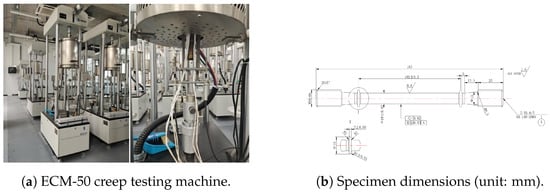
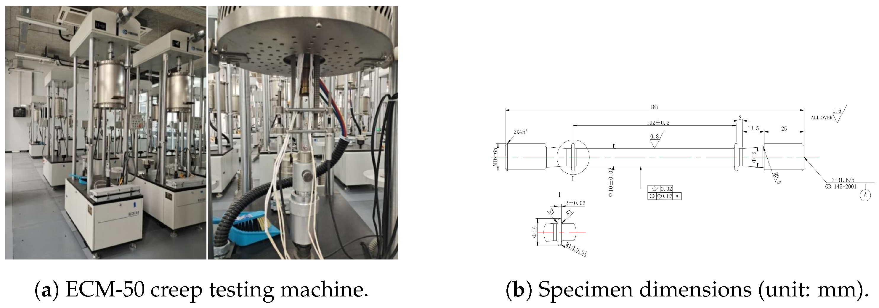
Uniaxial tensile creep tests were conducted in accordance with GB/T 2039-2012 [33] (Metallic materials—Uniaxial tensile creep testing method) using an ECM-50 metal high-temperature creep and stress rupture testing machine (Changchun Kexin Test Instrument Co., Ltd., Changchun, China) with a maximum capacity of 50 kN, force control accuracy ≤, temperature fluctuation <±1 °C during the steady stage, and deformation measurement resolution of 0.5 μm. The testing apparatus and specimen geometry are shown in Figure 1. During each test, the specimen was heated to the prescribed temperature at a rate of 0.67°C/min, held for 2 h to ensure thermal equilibrium, and then loaded to the target stress within 2 min. Creep strain was recorded continuously for durations exceeding 500 h to capture the steady-state creep rate.
Figure 1.
Experimental apparatus and specimen configuration [34].
The two alloys tested (2A12-T4 aluminum alloy and ZM6 magnesium alloy) exhibit distinct mechanical properties, summarized in Table 1. Both materials have comparable elastic moduli (), but differ markedly in yield strength (323 MPa vs. 128 MPa) and ductility (15.16% vs. 6.42% elongation).
Table 1.
Mechanical properties of the two alloys.
An orthogonal experimental design covering temperature and stress as two factors with four levels each was adopted. Table 2 summarizes all 13 experimental conditions and the corresponding data characteristics. Each experimental condition corresponds to a single uniaxial creep specimen; the point counts in Table 2 (14–100) therefore refer to strain–time samples recorded continuously from one creep curve, not to replicate specimens.
Table 2.
Summary of experimental conditions and data characteristics.
The experimental data exhibit two key contrasts. First, the data volume differs markedly between the two alloys: 2A12-T4 yields 96–100 data points per condition with approximately uniform time intervals ( h), whereas ZM6 provides only 14–34 points per condition with non-uniform temporal spacing. Second, the strain magnitudes differ by two orders of magnitude, for 2A12-T4 versus for ZM6, reflecting fundamentally different creep mechanisms and initial loading responses.
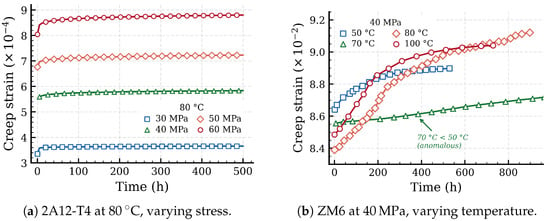
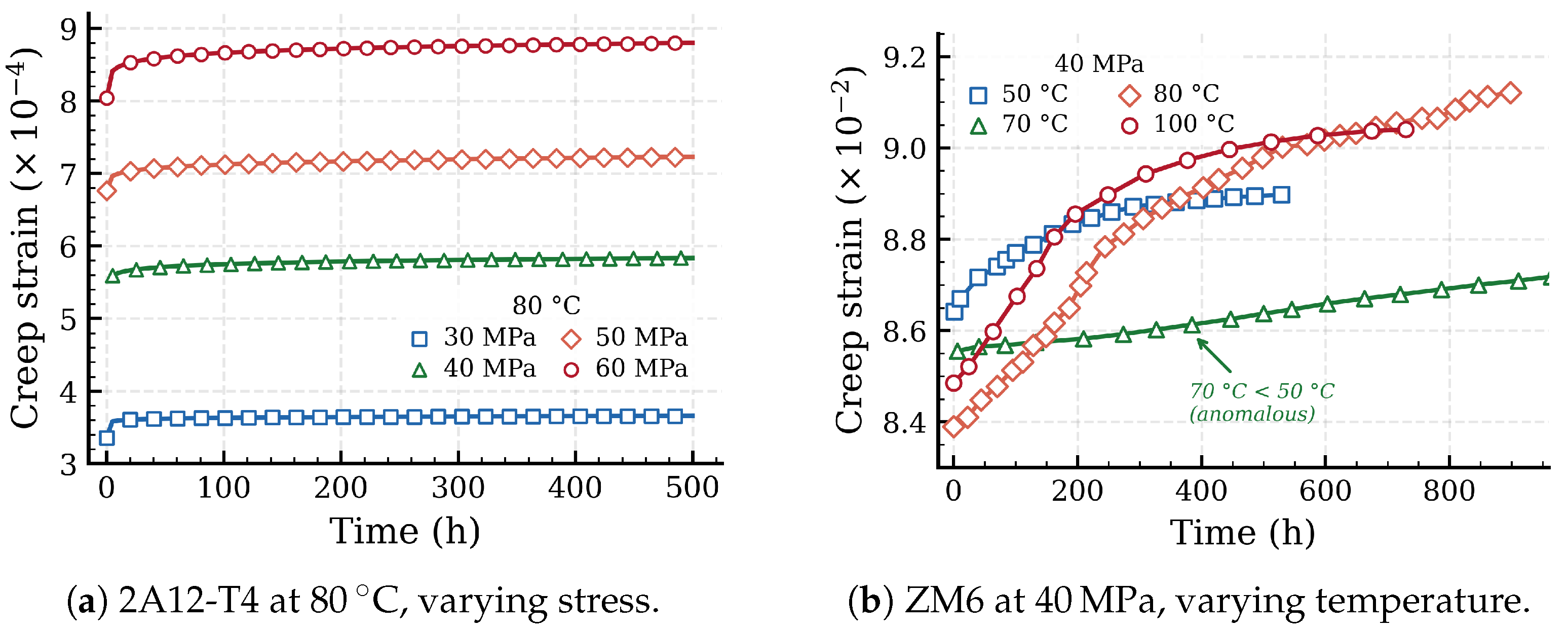
Figure 2 presents representative creep curves for selected conditions. For 2A12-T4 alloy at 80 °C under varying stress levels (Figure 2a), the curves exhibit a clear primary-to-steady-state transition with creep strain increasing monotonically with applied stress. For ZM6 alloy at 40 MPa under varying temperatures (Figure 2b), a non-monotonic temperature dependence is evident: the creep strain at 70 °C is lower than at both 50 °C and 80 °C, an anomaly that will be discussed further in Section 2.2.2.
Figure 2.
Representative experimental creep curves. The non-monotonic temperature dependence in ZM6 (70 °C curve below 50 °C) is highlighted.
This natural contrast in data availability and physical behavior provides an ideal testbed for evaluating the data efficiency of physics-informed approaches. The following subsections present the constitutive frameworks that govern these creep processes.
2.2. Creep Constitutive Frameworks
Under constant uniaxial stress and temperature T, the creep strain evolves according to an ordinary differential equation (ODE) of the general form:
where D denotes an internal damage variable characterizing the progressive degradation of material integrity, and represents material-specific constitutive parameters. For alloys where damage accumulation is negligible, D can be omitted and the right-hand side reduces to a direct function of stress and temperature.
2.2.1. 2A12-T4 Aluminum Alloy
Metallographic analysis of 2A12-T4 alloy before and after creep reveals that the dominant mechanism at 50–100 °C is thermally activated diffusion [3]. Comparison of post-creep specimens with virgin material shows a reduction in blocky second-phase particles and no measurable grain coarsening, confirming that damage accumulation is negligible under the tested conditions. The creep rate is therefore described by an Arrhenius-type power-law relationship
where , , and are material constants, is the applied stress (MPa), and T is the absolute temperature (K). Parameter fitting based on the experimental steady-state creep rates yields , , and .
The total creep strain at time t is obtained by integration:
where denotes the initial strain due to instantaneous elastic loading. Since no significant damage evolution is observed under the tested conditions, the damage variable D is omitted, and the creep rate remains constant for fixed and T.
This steady-state formulation does not explicitly model the primary (decelerating) creep transient, which manifests as the initial rapid strain increase observed in the experimental data. Capturing this transient is one of the motivations for introducing a data-driven component through DC-PINN.
2.2.2. ZM6 Magnesium Alloy
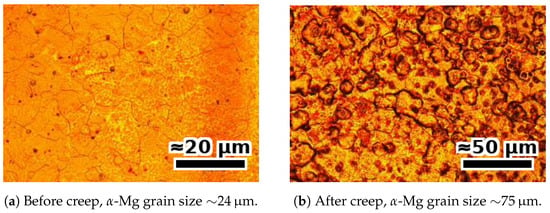
The creep behavior of ZM6 alloy is governed by a fundamentally different mechanism. Metallographic analysis reveals that under the combined effects of temperature and stress, atomic diffusion and grain boundary migration are accelerated, causing second-phase particles at grain boundaries and within grains to coarsen. This coarsening reduces the number of grain boundaries, weakens their impedance to dislocation motion, and thereby accelerates creep deformation [15,16]. The microstructural evidence is illustrated in Figure 3. For Mg–RE alloys with melting temperature , the homologous temperature in the tested range is –. This falls within the established dislocation glide–climb regime of Mg alloy creep [16], where the Sandström dislocation framework [14] remains applicable. The contribution of long-term stress relaxation of residual assembly stresses is implicitly absorbed by the data term of the proposed framework rather than ignored.
Figure 3.
Metallographic images of ZM6 alloy showing significant grain coarsening during creep.
Based on the dislocation density evolution framework [13,14], when the material reaches steady-state creep, the internal dislocation density remains approximately constant. Following the approach of expressing the stress-dependent terms as a hyperbolic sine function to ensure accuracy over a wide stress range [12], the steady-state creep rate is
where A and B are material constants, is the temperature-dependent activation energy, and is the universal gas constant.
The dominant damage mechanism, grain coarsening, follows the Ostwald ripening law:
where r is the grain radius at time t, is the initial radius, and K is the coarsening rate constant. A dimensionless damage variable D is defined to quantify the effect of grain coarsening on creep rate:
Here, D is a grain-size-based variable that admits direct microstructural interpretation, not a phenomenological softening parameter. Its evolution is therefore governed by the kinetics of grain coarsening (Equation (5)) rather than by an empirical damage law.
With the corresponding damage evolution rate:
Incorporating the damage variable into the steady-state creep rate, the complete CDM constitutive model for ZM6 alloy is
where C is a material constant related to effective stress redistribution under damage. The constitutive parameters A, B, C, , and in Equation (8) are obtained by least-squares fitting of the steady-state portion of experimentally measured creep curves at the calibration conditions, following the procedure described in [15,16]. The constitutive parameters are listed in Table 3.
Table 3.
Constitutive model parameters for ZM6 magnesium alloy.
The activation energies at the three tested temperatures are
For intermediate temperatures not explicitly listed above (e.g., , corresponding to 70 °C), is obtained by linear interpolation between adjacent calibration points. The resulting value falls between the 50 °C and 80 °C calibration values. Similarly, the empirical functions and defined below are evaluated at the corresponding temperature. We acknowledge that an Arrhenius-form interpolation of versus would be theoretically preferable for activation energies, but the three available calibration points are insufficient to constrain a more refined dependence. Any residual approximation in is absorbed by the data-fidelity term during training; the reproduction of the non-monotonic ranking observed at 70 °C (see Section 4) confirms that this approximation is not the limiting factor in prediction accuracy.
The effective stress parameter C and normalized coarsening rate are empirical functions of stress and temperature:
where T is in Kelvin and in MPa.
ZM6 alloy exhibits a non-monotonic temperature dependence of creep strain. Under constant stress of 40 MPa, the creep strain at 70 °C is lower than at both 50 °C and 80 °C (see Figure 2b). This anomaly arises from the competition among the temperature-dependent activation energy , the effective stress parameter , and the grain coarsening rate : the non-monotonic variation in across the tested temperature range (Equation (9)) combines with the quadratic temperature terms in Equations (10) and (11) to produce a net reduction in the effective creep driving force near 70 °C. This behavior, which contradicts typical thermal activation expectations, poses a stringent validation case for physics-informed models and will be revisited in Section 4.
2.3. Problem Statement
Given the constitutive frameworks established above, the creep strain prediction problem for each experimental condition (fixed , T) is to learn a mapping that simultaneously
- (i)
- fits the sparse experimental observations , where N ranges from 14 to 100;
- (ii)
- (iii)
- for ZM6, also satisfies the coupled damage evolution (Equation (7));
- (iv)
- respects physical constraints including strain monotonicity () and initial conditions ().
Requirements (i) and (ii)–(iv) are inherently in tension: a purely data-driven model satisfying (i) alone may violate physical consistency, while a purely physics-based model satisfying (ii)–(iv) alone cannot adequately fit the data, particularly during the primary creep transient. The DC-PINN framework introduced in the next section is designed to balance these competing objectives through a unified loss function that integrates data fidelity with hierarchical physics constraints.
3. Methodology
3.1. Framework Overview
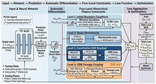
DC-PINN addresses the four requirements stated in Section 2.3 by learning the creep strain mapping from a unified loss function combining data fidelity with hierarchical physics constraints. Figure 4 illustrates the overall architecture.
Figure 4.
Overview of the DC-PINN framework. The neural network predicts , and automatic differentiation yields . Four levels of physics constraints are enforced through the composite loss function. For ZM6 alloy, Level 4 (CDM damage evolution) provides an additional differential constraint coupling with the damage state . In the schematic, solid arrows denote forward computation flow; the ⊕ symbol denotes the weighted summation defined in Equation (22); and the color coding distinguishes data fidelity terms, physics-constraint terms, and the damage-coupling branch active only for ZM6.
The framework consists of three components: (i) a neural network that takes normalized time as input and outputs the predicted creep strain (Section 3.2); (ii) a hierarchical set of physics constraints enforced through automatic differentiation and penalty terms in the loss function (Section 3.3); and (iii) a composite loss function with adaptive weighting that balances data fitting against physical consistency (Section 3.4).
A separate network is trained for each experimental condition (fixed , T), as the constitutive parameters and damage kinetics are condition-specific. This per-condition strategy avoids the need to learn cross-condition generalization from sparse data, and instead focuses the network capacity on capturing the temporal evolution within each condition.
3.2. Neural Network Architecture
For each condition (, T), the PINN takes normalized time as input and outputs a scalar , which is then rescaled to the physical domain:
where and are respectively the minimum and maximum strains observed in the experimental data. This affine mapping centers the learning target near zero, improving gradient conditioning and training stability. The input normalization similarly prevents large magnitudes from biasing the initialization.
The network is a fully connected feedforward architecture with L hidden layers, each containing H neurons and using the hyperbolic tangent (tanh) activation function. The tanh activation is chosen for its smoothness and bounded output, which ensures that the strain derivative obtained via automatic differentiation is well-defined and continuous, a requirement for evaluating the ODE residual constraints.
Given the low-dimensional input space (scalar t) and the smooth nature of creep curves, a compact network (, ) is adopted. This moderate capacity is intended to prevent overfitting on the sparse datasets while retaining sufficient flexibility to capture the primary-to-steady-state transition.
3.3. Hierarchical Physics Constraints
The physics constraints are organized into four levels of increasing physical depth, indexed in the order they are activated by the ablation sequence (B1 → B2 → B3 → B4) in Section 4: Level 1 enforces initial and boundary conditions, Level 2 enforces strain monotonicity, Level 3 enforces the constitutive ODE residual, and Level 4 enforces CDM damage coupling. Table 4 summarizes the four levels and Figure 4 visualizes their integration into the loss function; the loss-term column of the table identifies the corresponding penalty in Equation (22), while the right-hand branches in Figure 4 show how each level is enforced through automatic differentiation and penalty terms.
Table 4.
Hierarchical physics constraint architecture of DC-PINN, indexed by ablation activation order.
3.3.1. Level 1: Initial and Boundary Conditions
The initial strain , corresponding to the instantaneous elastic response upon loading, is enforced as a loss penalty:
where is taken from the first experimental data point. For conditions where the first measurement occurs at a nonzero time (e.g., 2A12-T4 at 100 °C/50 MPa, where recording begins at h), the initial condition is applied at the earliest available measurement.
In addition, for conditions where a reliable steady-state creep rate has been experimentally determined, a terminal rate constraint can be imposed:
This provides an anchor at the end of the time domain, discouraging the network from drifting away from the physically expected asymptotic behavior. The terminal rate term is not redundant with the ODE residual introduced at Level 3. The ODE residual penalizes the squared difference between the predicted rate and the full constitutive rate at all collocation points, whereas provides a low-variance anchor against an independently measured experimental value at the time-domain boundary. The two terms remain complementary even after Level 3 is activated, since the experimental steady-state rate carries information not present in the analytical f. For conditions where is unavailable, deactivates this term without affecting the rest of the architecture.
3.3.2. Level 2: Strain Monotonicity
Under constant tensile stress and temperature, creep strain is physically non-decreasing. This constraint is enforced by penalizing negative strain rates at the collocation points:
This constraint complements the ODE residual introduced next (Level 3): Level 3 guides the strain rate toward the constitutive prediction, whereas Level 2 provides a lower bound that prevents physically inadmissible negative rates, which may arise during early training iterations or in data-sparse regions. Monotonicity is implemented as a soft penalty rather than an architectural hard constraint, allowing the network to recover from transient violations during early training while preserving expressive capacity. In the extrapolation region where no data is available, non-physical predictions of are suppressed by the joint action of two mechanisms. First, the ODE residual at Level 3 supplies a strictly positive analytical rate at all admissible damage states , providing an effective lower bound. Second, the monotonicity penalty squared form yields a finite gradient even for small violations, biasing the network away from the inadmissible region. Empirically, the joint enforcement reduces monotonicity-violation rate from 8–12% (B1, data-only) to below 0.5% (B2–B4), as quantified in Section 4.5.
3.3.3. Level 3: Constitutive ODE Residual
The most informative physics constraint requires that the network’s predicted strain rate be consistent with the constitutive rate law. Given the trained network , the strain derivative is computed via automatic differentiation, and the ODE residual is defined as
where is the network prediction and is the constitutive rate function.
For 2A12-T4, the rate function is the Arrhenius law (Equation (2)), which is constant for fixed and T. For ZM6, the rate function is the CDM model (Equation (8)), which depends on time through the damage term .
The residual is evaluated at a set of collocation points uniformly sampled over . These collocation points are independent of the experimental data points and can be chosen at higher density, providing additional physics supervision without requiring extra experimental measurements. The corresponding loss term is
This constraint is enforced as a soft penalty rather than a hard constraint, acknowledging that the constitutive model is an approximation, particularly during the primary creep transient, where the steady-state formulation is known to be inaccurate (see Section 2.2). The penalty strength is controlled by the loss weight discussed in Section 3.4.
3.3.4. Level 4: CDM Damage Evolution Coupling
For ZM6 alloy, the constitutive rate (Equation (8)) depends on the damage state through the term . While the Level 3 residual implicitly involves damage, an explicit constraint on the damage evolution provides additional physical regularization. Since (Equation (7)) implies a linear analytical solution , this constraint can be enforced by requiring the effective damage inferred from the network prediction to be consistent with the Ostwald ripening kinetics.
Specifically, given the network’s predicted strain rate , the effective damage is obtained by inverting Equation (8). Defining the normalized rate , the effective damage state is
The damage consistency residual then measures the deviation between this network-inferred damage and the Ostwald ripening prediction:
and the corresponding loss term is
This coupling between strain evolution and damage state through a differential constraint distinguishes DC-PINN from existing PINN approaches in the creep domain, which embed physics only through feature engineering or scalar penalty terms. For 2A12-T4 alloy, where no significant damage evolution is observed, this constraint level is omitted. A soft-penalty formulation is essential here for a reason specific to inverted constitutive constraints. Because is obtained by inverting Equation (8), any systematic error in the hyperbolic-sine model would be propagated to and then re-enforced on the network through . The soft penalty allows the data-fidelity term to dominate in data-dense regions, so the network can deviate from the analytical damage law when experimental evidence demands it. The CDM-coupling residual is therefore a physically grounded regulariser that biases the network toward Ostwald-ripening kinetics in data-sparse regions, not a hard reproducer of analytical f. Empirically, this separation is observable in Section 4: the gap between B4 (DC-PINN with full damage coupling) and B5 (analytical CDM evaluated at fitted parameters) on ZM6 quantifies the correction that the data term contributes beyond the analytical model.
3.4. Composite Loss Function and Training Strategy
The data fidelity loss measures the discrepancy between network predictions and experimental observations:
The total loss function combines data fidelity with all applicable physics constraints:
where , , , , and are non-negative weights controlling the relative importance of each constraint. For 2A12-T4 alloy, since the damage evolution constraint is not applicable.
Selecting appropriate loss weights is critical, as imbalanced weights may cause the physics loss to dominate and suppress data fitting, or vice versa. A two-phase training strategy is adopted to mitigate this issue. In the first phase, all physics constraint weights are set to zero (), and the network is trained with data loss only for a warm-up period, allowing it to approximate the general shape of the creep curve. In the second phase, physics constraints are activated with initial weights determined by normalizing each loss component to comparable magnitudes at the transition point. The weights are subsequently adjusted via a gradient-norm balancing scheme [35,36] to prevent any single loss term from dominating the gradient updates. The resulting loss-weight values are reported in Table 5 for two representative conditions: 2A12-T4 at 80 °C/50 MPa (data-rich, ) and ZM6 at 50 °C/20 MPa (data-sparse, ). The two alloys differ in strain magnitude by approximately two orders of magnitude (Section 2.1), which propagates through the loss components and leads to the substantially larger and for ZM6 reported in the table. Gradient-norm balancing [35,36] was selected over alternatives such as the adaptive inverse-Dirichlet weighting strategy because the dominant constraint shifts between Phase 1 and Phase 2, and gradient-norm balancing tracks the gradient magnitudes directly rather than the loss magnitudes; the data-sparse ZM6 condition (right block of Table 5) confirms that this choice maintains stable training under extreme data sparsity.
Table 5.
Loss-function weights per alloy and per training phase, for two representative conditions. Phase 1 (epochs 1–5000) is the warm-up with data loss only; Phase 2 (epochs 5001–20,000) activates physics constraints with weights initialised by gradient-magnitude normalisation and adapted via gradient-norm balancing.
The network is trained using the Adam optimizer with an initial learning rate of , decayed by a factor of 0.5 every 2000 epochs, for a total of 20,000 epochs. The number of collocation points is set to , uniformly sampled over and resampled every 1000 epochs to improve coverage of the time domain.
As summarized in Table 4, the key difference between the two alloys lies in Level 4: ZM6 activates CDM damage coupling, whereas 2A12-T4 does not, reflecting the distinct damage mechanisms identified in Section 2.2. The DC-PINN framework defined above was evaluated in Section 4 through systematic experiments designed to quantify the contribution of each constraint level.
4. Experiments
4.1. Experimental Setup
To systematically evaluate the contribution of each physics constraint level, five baseline models are constructed, spanning a spectrum from purely data-driven to purely physics-based (Table 6). B1 is the purely data-driven reference. B2–B4 form an incremental sequence, each adding one or more constraint levels atop the previous, enabling direct quantification of each layer’s marginal contribution. B5 is the purely physics-based reference, where the constitutive equations are evaluated directly with fitted parameters. For 2A12-T4, B3 and B4 are equivalent since Level 4 (CDM damage coupling) is not applicable. The ablation progression B1 → B2 → B3 → B4 follows the Level numbering in Table 4: B2 activates Levels 1 and 2 (initial/boundary conditions and monotonicity), B3 activates Level 3 (constitutive ODE residual) in addition, and B4 activates Level 4 (CDM damage coupling) in addition. This ordering isolates the marginal contribution of each successively deeper physics layer.
Three complementary metrics are adopted: the coefficient of determination , the root mean square error (RMSE), and the normalized RMSE (NRMSE ), where the normalization by the strain range enables cross-condition and cross-alloy comparison. All neural network-based models (B1–B4) share the same architecture described in Section 3.2: 4 hidden layers with 32 neurons, tanh activation, trained for 20,000 epochs with Adam optimizer (initial learning rate , halved every 2000 epochs) and collocation points. Each experiment is repeated 5 times with different random seeds; the mean is reported. All models are implemented in PyTorch 2.6.0+cu126 (PyTorch Foundation, San Francisco, CA, USA).
4.2. Overall Performance Comparison
Table 7 presents the values across all 13 conditions. Several patterns emerge. First, across both alloys, incorporating physics constraints consistently improves prediction accuracy: the average for 2A12-T4 increases from 0.984 (B1) to 0.996 (B3), while for ZM6 the improvement is substantially larger, from 0.916 (B1) to 0.985 (B4). This disparity (an absolute gain of 0.012 versus 0.069) reflects the greater value of physics constraints under data-sparse conditions. Second, the analytical CDM model (B5) achieves average of 0.952 for 2A12-T4 and 0.943 for ZM6, lower than the corresponding PINN variants. This gap originates from the rigid functional form of B5: although the phenomenological model captures the general shape of the primary-to-steady-state transition, its fixed parametric structure produces systematic overshoot in the transition region where the creep rate decelerates most rapidly, corroborating the limitation identified in Section 2.2.
Table 7.
Overall performance comparison (). For 2A12-T4, B3 and B4 are identical. Best results in bold.
An interesting crossover is observed between B2 (weak physics + data-driven) and B5 (full physics, no data fitting). For ZM6 under the sparsest conditions (50 °C/20 MPa, 14 points; 100°C/40 MPa, 15 points), B5 outperforms B2, indicating that physical model knowledge compensates for data scarcity more effectively than weak constraints alone. Conversely, for the densest ZM6 conditions (80 °C/30 MPa, 30 points; 80 °C/40 MPa, 34 points), B2 surpasses B5, suggesting that sufficient data allow the flexible data-driven component to outweigh the accuracy limitations of the fixed-form analytical model. This crossover supports the design of DC-PINN (B4), which combines both strengths and consistently outperforms all baselines regardless of data volume.
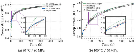
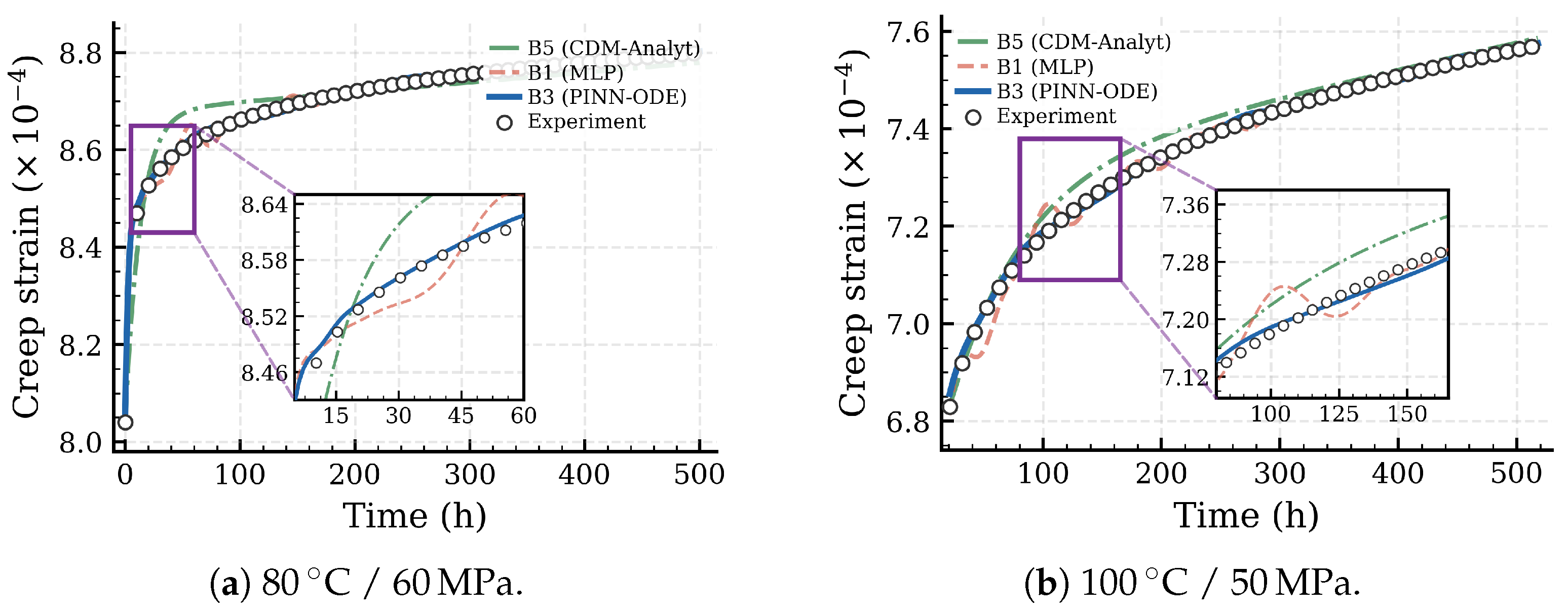
Figure 5 compares predicted creep curves for two representative 2A12-T4 conditions. The 80 °C/60 MPa case (Figure 5a) exhibits the largest strain increment and the most pronounced primary-to-steady-state transition among the tested conditions. As highlighted in the inset, B3 closely tracks the experimental data through the transition region, while B1 reproduces the overall trend but shows local deviations where the creep rate changes most rapidly. B5 captures the general curvature yet systematically overshoots the data during the transition, reflecting the limited flexibility of its fixed exponential-plus-linear functional form. At 100 °C/50 MPa (Figure 5b), which has the highest temperature and a delayed recording start ( h), the inset reveals the mid-time region (–170 h) where model differences are most evident: B3 maintains tight agreement with the data, B5 lies consistently above the experimental curve, and B1 exhibits oscillatory deviations around the true trajectory.
Figure 5.
Predicted vs. experimental creep curves for 2A12-T4 alloy. Solid blue: B3 (PINN-ODE); dashed orange: B1 (MLP); dash-dotted green: B5 (CDM-Analyt); open circles: experimental data. Insets zoom into the transition region where model differences are most pronounced.
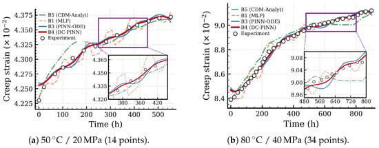
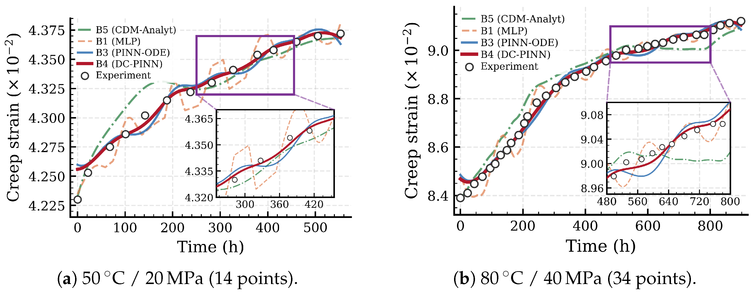
Figure 6 presents the comparison for ZM6, where the benefit of CDM damage coupling becomes visually apparent. For 50 °C/20 MPa (Figure 6a), with only 14 data points, B1 exhibits pronounced oscillations that persist throughout the time domain, reflecting overfitting to the sparse and unevenly spaced measurements. B5 reproduces the general ascending trend but drifts below the experimental data in the late region, as highlighted in the inset (–450 h). B3 substantially reduces these deviations, and B4 (DC-PINN) achieves the closest agreement, tracking the experimental trajectory most faithfully in the inset region. For 80 °C/40 MPa (Figure 6b), with 34 points and the longest time span (898 h), the advantage of damage coupling is most clearly revealed in the late-time inset (–800 h): B4 maintains tight agreement with the experimental data, whereas B3 shows mild deviations, B5 lies systematically below the data due to accumulated model error, and B1 continues to oscillate around the true trajectory. The non-smoothness visible in the B1 curves of Figure 5 and Figure 6 is a consequence of data-driven interpolation between widely spaced training points: with no physics constraint pulling the prediction toward the constitutive solution, B1 produces oscillations whose amplitude grows where the inter-point gap is largest. The mild non-smoothness occasionally visible in B3 and B5 on Figure 6 originates from a different mechanism, namely the piecewise reproduction of the CDM rate’s damage-driven slope changes in data fidelity-dominated regions, which is bounded by the analytical rate f rather than unconstrained. The 8–12% monotonicity-violation rate of B1 versus below 0.5% for B2–B4 quantifies the magnitude of this difference (Section 4.5).
Figure 6.
Predicted vs. experimental creep curves for ZM6 alloy. Bold red solid: B4 (DC-PINN, proposed); blue solid: B3 (PINN-ODE); orange dashed: B1 (MLP); green dash-dotted: B5 (CDM-Analyt); open circles: experimental data. Insets zoom into the late-time region where the CDM damage coupling provides the most pronounced improvement.
4.3. Ablation Study on Physics Constraints
The ablation study follows the progression B1 → B2 → B3 → B4, with each step adding one constraint level. Table 8 reports the incremental improvement () at each step, averaged over all conditions within each alloy. The total improvement from B1 to the best model is +0.012 for 2A12-T4 and +0.069 for ZM6, confirming that physics constraints are disproportionately valuable under data-sparse conditions.
Table 8.
Ablation study: average incremental improvement at each constraint level.
The B1→B2 step eliminates physically inadmissible negative strain rates and anchors the curve at the initial loading point. The improvement for ZM6 (+0.027) is 4.5 times that for 2A12-T4 (+0.006), reflecting the greater prevalence of non-physical artifacts when B1 operates on sparse data. Inspection of individual B1 predictions on ZM6 confirms that non-monotonic oscillations occur primarily in the mid-time region where data points are most widely spaced.
The B2 → B3 step introduces the constitutive ODE residual, providing differential-equation-level supervision through collocation points across the entire time domain. This step produces the same average gain as B1 → B2 for both alloys, but the improvement is qualitatively different: while monotonicity prevents gross violations, the ODE residual actively guides the strain rate toward the constitutive prediction, resulting in more accurate steady-state behavior and smoother primary-to-steady-state transitions.
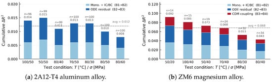
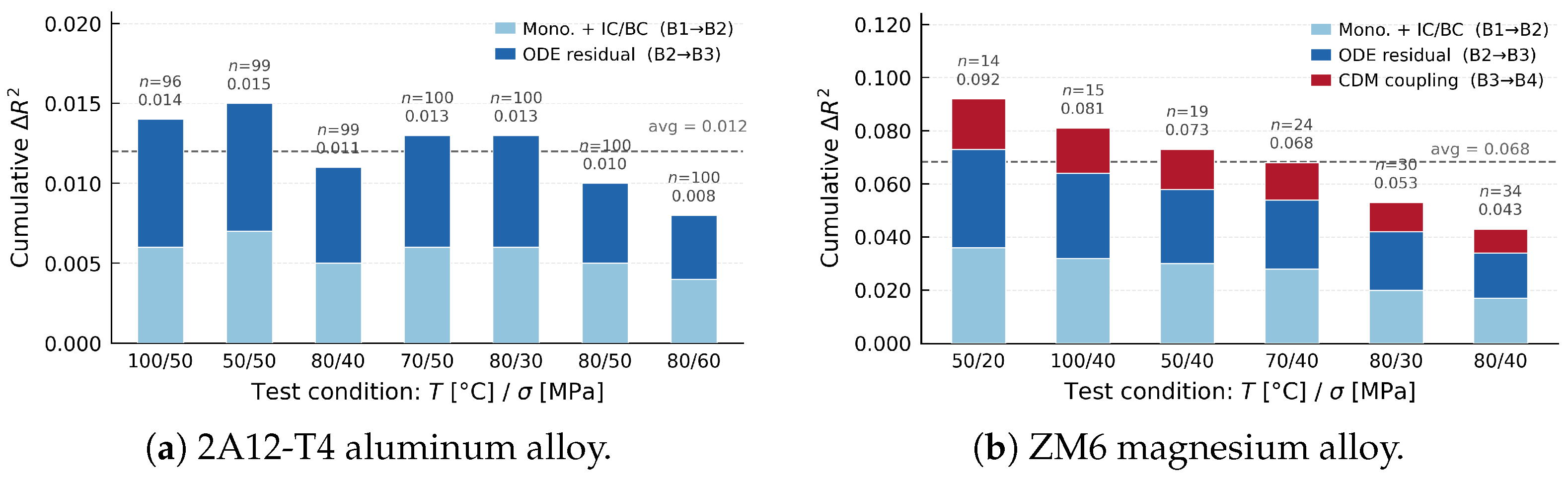
The B3 → B4 step, applicable only to ZM6, adds the CDM damage evolution coupling. The resulting of +0.015 constitutes 22% of the total improvement from B1 to B4. While smaller in magnitude than the ODE residual contribution, this gain is concentrated in the late-time regime where damage accumulation becomes non-negligible. Condition-level analysis reveals that the B3 → B4 improvement is most pronounced for the 80 °C/40 MPa condition (longest time span, 898 h) and least for the 50 °C/20 MPa condition (shortest effective damage accumulation), consistent with the physical expectation that grain coarsening damage plays a greater role at longer durations and higher temperatures. Figure 7 visualizes the incremental contribution of each constraint level.
Figure 7.
Cumulative improvement from each constraint level, sorted by ascending data size n. Light blue: monotonicity + IC/BC (B1 → B2); dark blue: ODE residual (B2 → B3); red: CDM damage coupling (B3 → B4, ZM6 only). The dashed line marks the cross-condition average. The total improvement is inversely correlated with data availability, confirming that physics constraints yield the greatest benefit in the data-sparse regime.
4.4. Data Efficiency Analysis
To further quantify the relationship between data availability and the value of physics constraints, a controlled subsampling experiment is conducted: for each 2A12-T4 condition, the training data are randomly subsampled to 80%, 60%, 40%, and 20% of the original size, and the values of B1 and B3 are evaluated for each fraction.
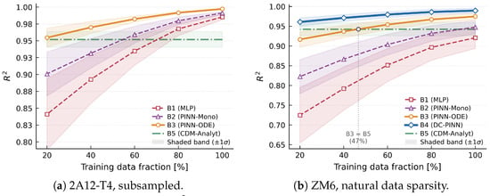
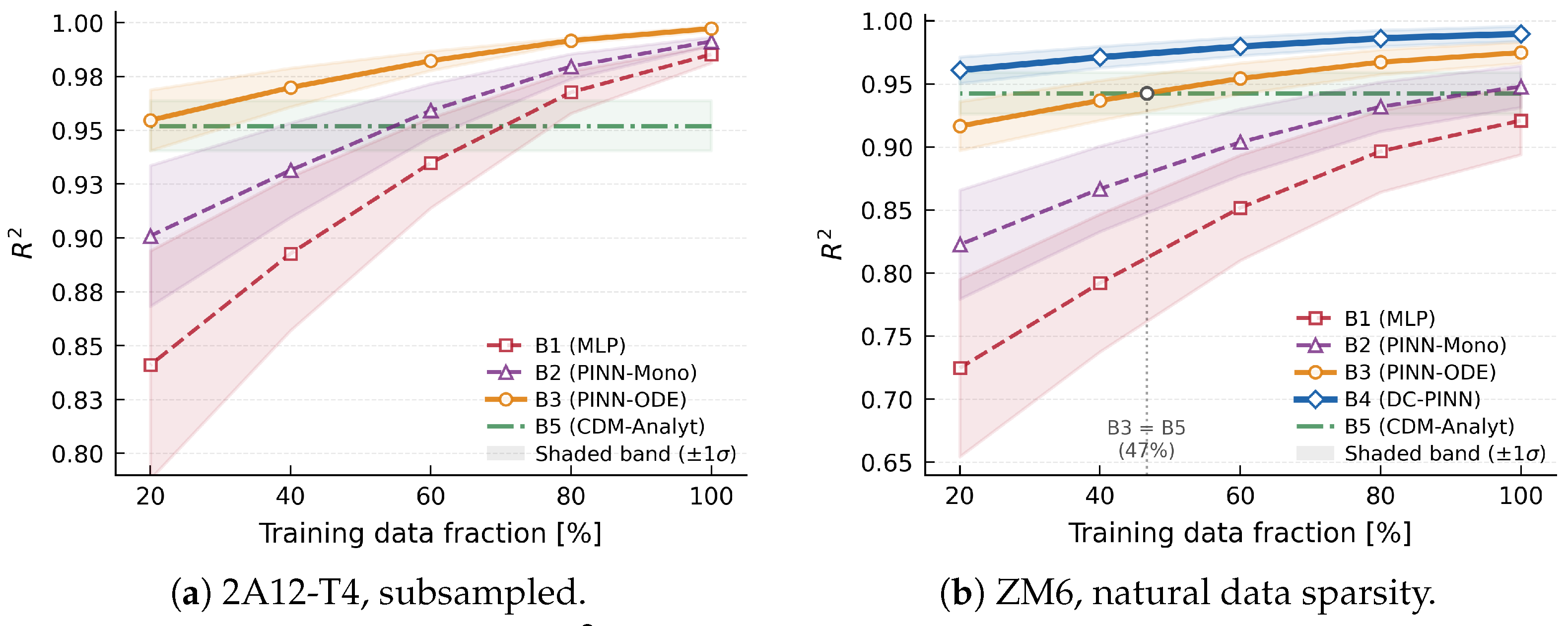
Figure 8 plots the average against training data fraction for both alloys; shaded bands indicate standard deviation across conditions. For 2A12-T4 (Figure 8a), B3 degrades gracefully: even at 20% data, it retains , marginally above B5 (). B1 drops from 0.985 to 0.841 (), and its error band widens substantially, confirming both its high sensitivity to data volume and increased variance across conditions. For ZM6 (Figure 8b), the situation is more revealing. As marked in the figure, B3 crosses below B5 at approximately 47% data, indicating that ODE constraints alone cannot compensate for severe data scarcity when the underlying physics involves damage evolution. B4 (DC-PINN), however, remains above B5 at every tested fraction, reaching at 20% data (still 0.018 above the analytical baseline) with a tight error band (). CDM damage coupling thus provides a regularization benefit that ODE residuals alone do not offer, raising the mean performance while also reducing its variability across conditions.
Figure 8.
Data efficiency: average vs. training data fraction. Horizontal dash-dotted green line: B5 (analytical constitutive model, data-invariant). Shaded regions denote standard deviation across conditions. In (a), fractions are obtained by random subsampling; in (b), each point represents one ZM6 condition at its full data size, with the fraction denoting the ratio of that condition’s data count to the maximum (34 points). The filled circle in (b) marks the fraction (≈47%) at which B3 drops below B5.
The crossover between B3 and B5 at ≈47% in Figure 8b has practical implications: it defines a data sufficiency threshold below which a physics-informed but damage-unaware model loses its advantage over a purely analytical one. Above this threshold, the neural network’s flexibility improves upon the rigid functional form of B5; below it, insufficient data cause the network to deviate, and the analytical model’s built-in physical structure becomes the safer choice. The widening gap between B3 and B5 at lower fractions (from at 40% to at 20%) shows how rapidly accuracy degrades without damage coupling. DC-PINN effectively eliminates this crossover, remaining 0.018 above B5 even at 20% data, ensuring that the PINN retains its advantage under extreme data scarcity.
4.5. Physical Consistency Analysis
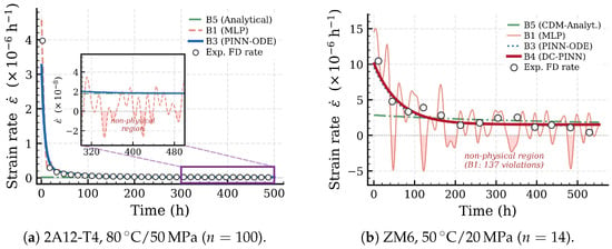
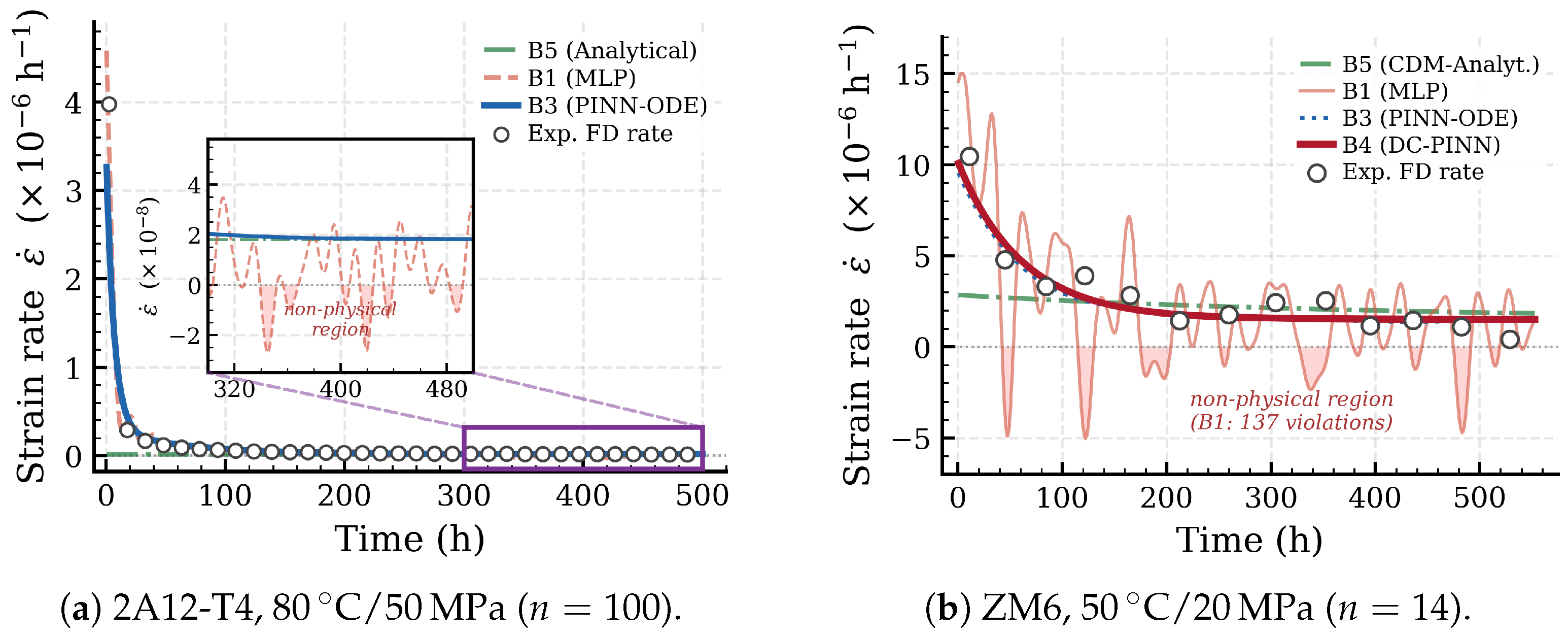
Under constant tensile loading, the creep strain must be non-decreasing. The fraction of collocation points where is computed for each model. For 2A12-T4, B1 produces a violation rate of approximately 3%, concentrated in the early time region, where the primary-to-steady transition creates steep gradients. For ZM6, the violation rate of B1 increases to 8–12%, with violations scattered across the time domain, owing to interpolation artifacts between sparse data points. All physics-constrained models (B2–B4) reduce the violation rate to below 0.5%, while B5 is monotonic by construction. Figure 9 visualizes this contrast for two representative conditions: the inset in Figure 9a magnifies the steady-state band where B1 violations are invisible at the main-axis scale, while Figure 9b reveals the more severe oscillations under extreme data sparsity (). B5 captures the steady-state rate but misses the primary creep transient entirely, producing a nearly constant rate from . The 8–12% monotonicity violation rate of the purely data-driven baseline carries direct engineering significance: in aerospace storage applications where creep strain is integrated over decades, any non-physical rate excursion accumulates as a permanent prediction error, motivating the joint enforcement of monotonicity and ODE residuals that characterizes DC-PINN.
Figure 9.
Physical consistency of predicted strain rates . B1 (MLP) produces oscillating rates with negative (non-physical) regions shaded in pink, whereas B3/B4 (PINN) maintain strictly positive rates through monotonicity enforcement and ODE constraints. The inset in (a) magnifies the steady-state band ( h−1) where B1 violations are invisible at the main axis scale. B5 (analytical) captures steady-state rates but misses the primary creep transient entirely.
Section 2.2.2 identified the non-monotonic temperature dependence of ZM6 creep strain as a stringent validation case: at 40 MPa, the 70 °C condition yields lower creep strain than both 50 °C and 80 °C. Since each condition is trained independently, this anomaly tests whether the per-condition PINN, informed by the correct temperature-dependent activation energy , produces predictions consistent with this counter-intuitive ordering. B5, B3, and B4 all reproduce the correct ranking, as their ODE constraints embed the experimentally determined values. In contrast, B1 (which lacks any temperature-dependent physics) does not reliably reproduce the correct ranking, because the strain differences between the 70 °C and 50 °C conditions are less than 2% and fall within B1’s prediction uncertainty. This illustrates how physics constraints ensure consistency even when purely statistical signals are weak.
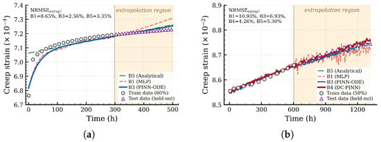
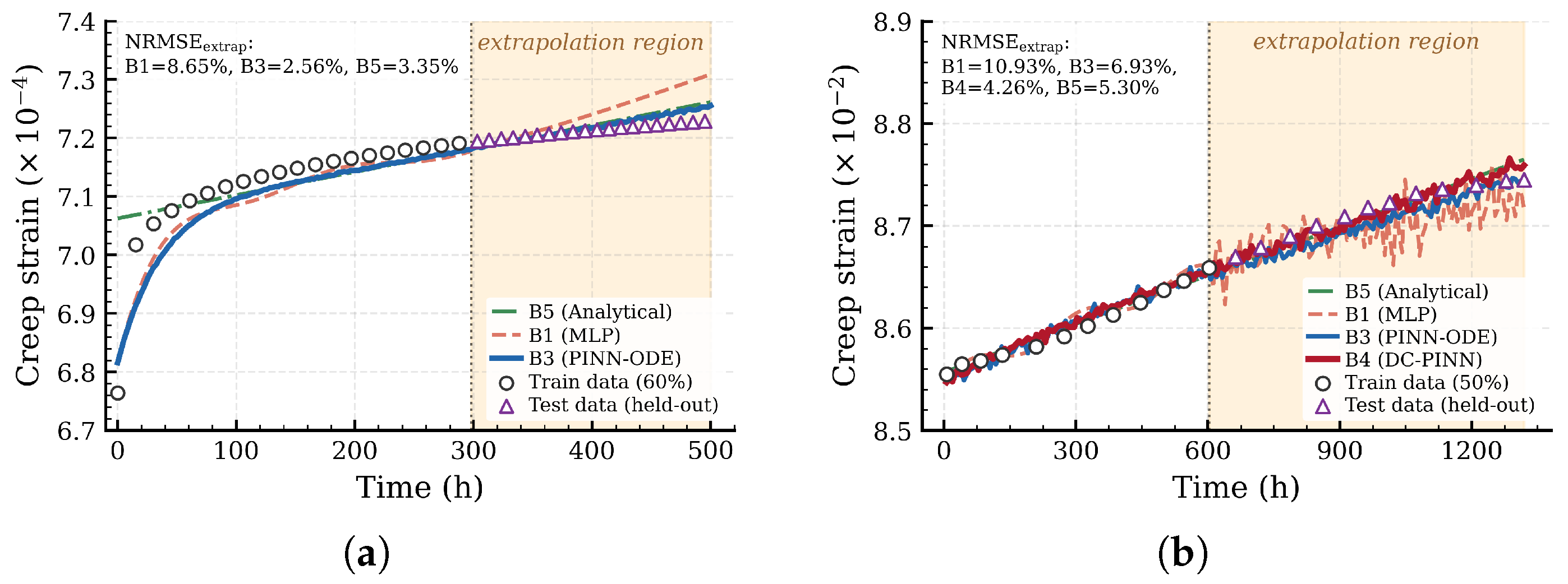
To assess extrapolation capability, two evaluation protocols are reported. A near-extrapolation calibration withholds the last 20% of each experimental curve during training and uses it as an out-of-sample test set; this protocol falls within the temporal regime sampled by the training data and therefore reflects the model’s interpolation-like extrapolation skill. A true-extrapolation protocol also trains on a contiguous early-time portion of two representative conditions (the first 60% of 2A12-T4 at 80 °C/50 MPa, h, training horizon ; and the first 50% of ZM6 at 70 °C/40 MPa, h, training horizon ) and asks the network to predict over the remaining 40–54% of the experimental window. The 2A12-T4 case stretches the prediction to ( h), and the ZM6 case stretches it to ( h). For the near-extrapolation protocol on 2A12-T4, B3 achieves an average NRMSE of approximately 2.5%, compared to 6.8% for B1 and 4.1% for B5. The ODE residual provides the model with a differential equation that continues to govern strain evolution beyond the training horizon, preventing the unconstrained drift that afflicts B1. For ZM6, DC-PINN (B4) further reduces the NRMSE to approximately 4.2%, compared to 5.8% for B3 and 12.1% for B1, as the CDM damage term grows linearly with time and increasingly influences the strain rate at longer durations. B5 achieves 5.5% NRMSE for ZM6, performing well in the steady-state extrapolation regime but carrying forward the accumulated error from the poorly fitted primary stage. For the true-extrapolation protocol, the relative ordering of the baselines is preserved and the absolute NRMSE rises as expected for a more demanding test. On 2A12-T4 (60% training), B3 (PINN-ODE) achieves NRMSE % over h, B5 (analytical) achieves 3.4%, and B1 (MLP) degrades to 8.7%. On ZM6 (50% training, with the prediction horizon stretching to over 1300 h), B4 (DC-PINN with damage coupling) achieves NRMSE %, B5 5.3%, B3 6.9%, and B1 10.9%. The widening B3→B4 gap on ZM6 (2.6 percentage points in true extrapolation versus 1.6 in near extrapolation) reflects the growing contribution of the damage coupling layer to long-time prediction accuracy. Figure 10 visualizes the two true-extrapolation experiments: in both panels the shaded region marks the held-out interval and the markers indicate experimental observations. Across both conditions the DC-PINN family (B3 for 2A12, B4 for ZM6) tracks the held-out data within experimental scatter, whereas the MLP baseline drifts away from the data envelope shortly after the training cutoff.
Figure 10.
True extrapolation experiments. The orange-shaded region indicates the held-out time interval; circles are training observations and triangles are held-out test observations. DC-PINN (B3 for 2A12-T4, B4 for ZM6) closely tracks the held-out data; B5 (analytical) provides a competitive baseline in steady-state regions; B1 (MLP) exhibits noticeable drift in the extrapolation interval. (a) 2A12-T4, 80 °C/50 MPa, first 60% (60/100 points) used for training; prediction extended to h. (b) ZM6, 70 °C/40 MPa, first 50% (12/24 points) used for training; prediction extended to h.
The horizons covered by the present experiments span hundreds to h, which is sufficient to validate the within-sample extrapolation behaviour of DC-PINN but does not, on its own, address the years-to-decades horizon characteristic of long-term aerospace storage. Multi-decade extrapolation is treated as a separate scientific question and is discussed in Section 5 as future work, including a time-temperature superposition (TTS) validation program that would couple short-duration tests at elevated temperatures with the DC-PINN framework at storage temperatures.
4.6. Discussion
The experiments validate three central findings. First, DC-PINN achieves across all ZM6 conditions and across all 2A12-T4 conditions, establishing that physics-informed learning produces accurate full-curve creep strain predictions for lightweight alloys under the low-temperature storage regime, which addresses the task-level and temperature-range gaps identified in Section 1. Second, the ablation study demonstrates that the CDM damage coupling contributes for ZM6, concentrated in the late-time regime; this physical process is absent from all prior PINN-creep frameworks, thereby addressing the constraint-depth gap. Third, the data efficiency analysis confirms that the total improvement from physics constraints is +0.069 for ZM6 (14–34 points) versus +0.012 for 2A12-T4 ( points), a 5.8-fold ratio that mirrors the approximately 5-fold difference in data density. A useful diagnostic for whether DC-PINN engages in non-trivial learning under data sparsity (as opposed to a disguised gradient-descent optimisation of the CDM parameters) is the gap between B4 (DC-PINN with full constraints) and B5 (analytical CDM evaluated at fitted parameters). On ZM6, B4 reaches an average while B5 reaches ≈0.943, giving that is preserved even on the sparsest 14-point condition. Because B5 already incorporates the full fitted constitutive model, the residual gap quantifies the correction that the data term contributes beyond pure CDM evaluation: DC-PINN absorbs systematic errors of the constitutive model in data-dense regions and falls back to physics-guided extrapolation elsewhere.
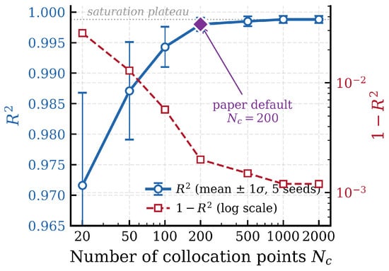
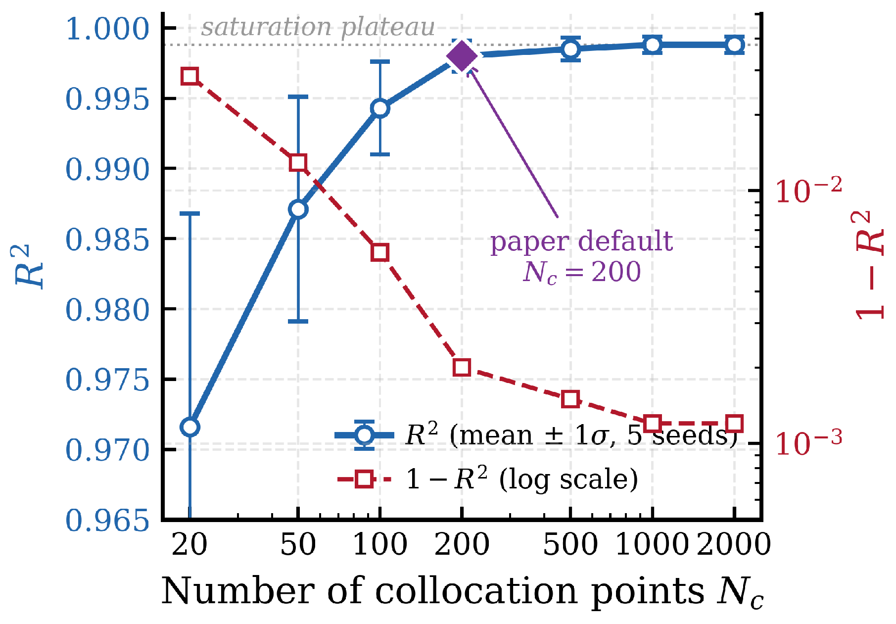
A complementary sensitivity sweep over the number of collocation points on the data-rich 2A12-T4 80 °C/50 MPa condition documents how the choice used throughout the experiments was reached. Figure 11 reports the mean and its dispersion across five seeds for . The saturation begins around , beyond which improvements fall below the seed-to-seed dispersion; the chosen corresponds to a collocation spacing of h, comfortably below the primary creep timescale h fitted from the experimental curve. Smaller values ( or 50) leave the ODE residual loss under-sampled in the primary-creep regime, which manifests both as a lower mean and as a wider seed-to-seed dispersion.
Figure 11.
Sensitivity of model accuracy to the number of collocation points on the 2A12-T4 80 °C/50 MPa condition. Error bars on (left axis, blue circles) span across five seeds; the complementary curve (right axis, red squares, logarithmic scale) makes the saturation behavior explicit. The paper’s default choice sits at the knee where further increases yield improvements below the seed-to-seed dispersion.
Several limitations merit discussion. The per-condition training strategy does not enable cross-condition generalization; predicting strain for an untested temperature-stress combination would require an extended architecture with and T as inputs. The constitutive parameters in the physics constraints are treated as fixed during training; joint optimization with network parameters could improve accuracy but introduces identifiability challenges. Finally, the framework addresses uniaxial loading only; extension to multiaxial stress states would require coupling with spatial field solvers.
5. Conclusions
This paper addressed the problem of predicting creep strain evolution in lightweight aerospace alloys under long-term storage conditions, where sparse experimental data and complex damage mechanisms limit the applicability of both purely physics-based and purely data-driven approaches. DC-PINN, a damage-coupled physics-informed neural network framework, was proposed that integrates CDM damage evolution equations as differential constraints into the learning process, forming a four-level hierarchical physics constraint architecture. The framework was validated on 13 experimental conditions spanning two alloys (2A12-T4 aluminum alloy with 7 conditions of points each, and ZM6 magnesium alloy with 6 conditions of 14–34 points each) at temperatures of 50–100 °C and stresses of 20–60 MPa.
The main findings are summarized as follows:
- 1.
- DC-PINN achieves across all 2A12-T4 conditions and across all ZM6 conditions, demonstrating that PINNs can produce accurate full-curve creep strain predictions (rather than scalar life estimates) for lightweight alloys in the low-temperature storage regime. Under a near-extrapolation protocol (last 20% of each curve withheld), DC-PINN achieves NRMSE of approximately 2.5% for 2A12-T4 and 4.2% for ZM6, compared to 6.8% and 12.1% for the purely data-driven baseline. Under a true-extrapolation protocol (first 60% / 50% of two representative conditions used for training), DC-PINN achieves 2.6% (2A12-T4, prediction to ) and 4.3% (ZM6, prediction to ) NRMSE in the held-out region. This extends the applicability of PINNs in creep modeling to a temperature range and prediction task not previously addressed in the literature.
- 2.
- The ablation study confirms that the CDM damage evolution coupling contributes an average of +0.015 for ZM6 alloy, accounting for 22% of the total physics-driven improvement. This contribution is concentrated in the late-time regime where grain coarsening damage becomes non-negligible, and is most pronounced for conditions with the longest experimental duration. The constitutive ODE residual (Level 3) provides the largest single-step improvement for both alloys, while boundary conditions and monotonicity (Levels 1–2) eliminate non-physical artifacts that are particularly prevalent under sparse data.
- 3.
- The value of physics constraints scales inversely with data availability. The total improvement from all physics constraints is +0.069 for ZM6 (14–34 points per condition) versus +0.012 for 2A12-T4 ( points), a 5.8-fold ratio. Subsampling experiments on 2A12-T4 further confirm that the performance gap between physics-informed and purely data-driven models widens as training data decrease, with the CDM damage coupling providing its largest marginal benefit at the lowest data fractions.
Several directions warrant future investigation. First, a multi-condition extension of DC-PINN is the planned next step: the per-condition strategy adopted here was a deliberate first-step choice to focus the network capacity on within-condition temporal evolution under sparse data; the next version will expand the input layer to accept and T as additional features, enabling interpolation and extrapolation across untested loading conditions and broadening the practical utility for storage life assessment. Second, jointly optimizing the constitutive parameters with the network weights (effectively solving an inverse problem) could reduce the dependence on prior parameter fitting and improve accuracy when the constitutive model is only approximately known. Third, coupling the present framework with spatial field solvers would enable extension to multiaxial stress states and complex component geometries encountered in real aerospace structures. Fourth, long-horizon validation at the years-to-decades scale relevant to aerospace storage is not directly addressed by the experiments reported here (which span up to h). A time-temperature superposition (TTS) protocol that combines short-duration tests at moderately elevated temperatures with DC-PINN predictions at storage-condition temperatures is a natural pathway: TTS-derived master curves at h could be cross-validated against the DC-PINN extrapolations reported in Section 4.5, providing an independent check on the framework’s long-horizon stability. Finally, the collocation point sensitivity sweep reported in Section 4.5 (Figure 11) shows that the default sits at the saturation knee for the present time horizons; revisiting this choice will be necessary when the framework is extended to substantially longer prediction windows, where finer collocation may be required to resolve damage-stage transitions.
Author Contributions
H.L.: Conceptualization, Methodology, Software, Investigation, Writing—original draft. S.H.: Resources, Data curation, Validation, Writing—review and editing. S.R.: Investigation, Formal analysis, Data curation, Writing—review and editing. B.Z.: Conceptualization, Methodology, Supervision, Writing—review and editing. C.Q.: Supervision, Project administration, Funding acquisition, Writing—review and editing. All authors have read and agreed to the published version of the manuscript.
Funding
This research was funded by National Natural Science Foundation of China grant number 52375237, National Science and Technology Major Project grant number J2022-IV-0012 and Hong Kong Polytechnic University and the Research Grants Council of the Hong Kong SAR grant number PolyU 15207221.
Data Availability Statement
Data will be made available on request.
Conflicts of Interest
The authors declare that they have no known competing financial interests or personal relationships that could have appeared to influence the work reported in this paper.
References
- Li, Q.; Lin, Y.; Wang, S.; Wang, S.; Zhu, X. Storage reliability assessment method for aerospace electromagnetic relay based on belief reliability theory. Appl. Sci. 2022, 12, 8637. [Google Scholar] [CrossRef] [Scilit]
- Shi, H.; Liu, R.; Chen, H.; Wang, W.; Zhou, J.; Chen, X.; Liu, K. Microstructural evolution and mechanical properties of zm6 (mg-nd-zr-zn) alloy fabricated by wire arc additive manufacturing. J. Alloys Compd. 2025, 1022, 180096. [Google Scholar] [CrossRef] [Scilit]
- Yan, J.; Cao, Z.; Zhang, W.; Jin, S.; Guo, Z.; Yuan, Y.; Ma, H. Research on the microscopic characteristics of low-cycle-fatigue and creep coupling in cast aluminum alloys for cylinder heads. Int. J. Fatigue 2025, 197, 108952. [Google Scholar] [CrossRef] [Scilit]
- Yu, W.; Zhan, L.; Xu, Y.; Chen, K.; Yang, Y.; Xu, L.; Peng, N.; Ma, B.; Liu, C.; Chen, Z. Temperature-dependent creep aging behavior of 2a14 aluminum alloy. J. Mater. Res. Technol. 2022, 19, 1343–1354. [Google Scholar] [CrossRef] [Scilit]
- Zhang, Y.; Hong, Y.; Li, H.; Zhang, D. Creep behavior and dynamic precipitation of highly heat-resistant mg alloy with low rare-earth content. J. Alloys Compd. 2024, 997, 174960. [Google Scholar] [CrossRef] [Scilit]
- Zhang, L.; Heng, L.; Tianjun, B.; Changhui, W.; Yang, G.; Chao, L. Advances and challenges on springback control for creep age forming of aluminum alloy. Chin. J. Aeronaut. 2022, 35, 8–34. [Google Scholar] [CrossRef] [Scilit]
- Liu, H.; Yu, H.; Guo, C.; Chen, X.; Zhong, S.; Zhou, L.; Osman, A.; Lu, J. Review on fatigue of additive manufactured metallic alloys: Microstructure, performance, enhancement, and assessment methods. Adv. Mater. 2024, 36, 2306570. [Google Scholar] [CrossRef] [Scilit]
- Raj, S. Power-law and exponential creep in class m materials: Discrepancies in experimental observations and implications for creep modeling. Mater. Sci. Eng. A 2002, 322, 132–147. [Google Scholar] [CrossRef] [Scilit]
- Wang, X.-Y.; Wang, X.; Zhang, X.-C.; Zhu, S.-F. Creep damage characterization of uns n10003 alloy based on a numerical simulation using the norton creep law and kachanov–rabotnov creep damage model. Nucl. Sci. Tech. 2019, 30, 65. [Google Scholar] [CrossRef] [Scilit]
- Yu, P.; Ma, W. A modified theta projection model for creep behavior of rpv steel 16mnd5. J. Mater. Sci. Technol. 2020, 47, 231–242. [Google Scholar] [CrossRef] [Scilit]
- Alang, N.; Nikbin, K. A new approach to predict creep rupture of grade 92 steel under multiaxial stress states. Int. J. Mech. Sci. 2019, 163, 105096. [Google Scholar] [CrossRef] [Scilit]
- Haque, M.S.; Stewart, C.M. Comparative analysis of the sin-hyperbolic and kachanov–rabotnov creep-damage models. Int. J. Press. Vessel. Pip. 2019, 171, 1–9. [Google Scholar] [CrossRef] [Scilit]
- Preußner, J.; Rudnik, Y.; Brehm, H.; Völkl, R.; Glatzel, U. A dislocation density based material model to simulate the anisotropic creep behavior of single-phase and two-phase single crystals. Int. J. Plast. 2009, 25, 973–994. [Google Scholar] [CrossRef] [Scilit]
- Sandström, R.; He, J.-J. Comments on creep-induced elemental redistribution at grain boundaries of 304l stainless steel–an experimental evidence for diffusional creep mechanisms. Scr. Mater. 2026, 278, 117256. [Google Scholar] [CrossRef] [Scilit]
- Fu, X.; Zhao, Z.; Yan, Z.; Zhong, Y.; Chen, D.; Zhang, R.; Liu, B.; Fang, Q.; Li, J. Multiscale microstructure-based constitutive modeling of high-temperature creep rupture in post-irradiated ods steels. J. Mater. Res. Technol. 2025, 36, 8037–8047. [Google Scholar] [CrossRef] [Scilit]
- del Valle, J.; Ruano, O. Separate contributions of texture and grain size on the creep mechanisms in a fine-grained magnesium alloy. Acta Mater. 2007, 55, 455–466. [Google Scholar] [CrossRef] [Scilit]
- Li, C.; Wan, M.; Wu, X.-D.; Huang, L. Constitutive equations in creep of 7b04 aluminum alloys. Mater. Sci. Eng. A 2010, 527, 3623–3629. [Google Scholar] [CrossRef] [Scilit]
- Mirzaei, A.; Dillon, S.J. An arrhenius mechanics model for polycrystalline plasticity and creep. Acta Mater. 2026, 305, 121831. [Google Scholar] [CrossRef] [Scilit]
- Miyano, Y.; Nakada, M. Accelerated testing methodology for durability of cfrp. Compos. Part B Eng. 2020, 191, 107977. [Google Scholar] [CrossRef] [Scilit]
- Gao, T.; Zhan, Z.; Hu, W.; Meng, Q. A novel damage mechanics and xgboost based approach for hcf life prediction of cast magnesium alloy considering internal defect characteristics. Int. J. Fatigue 2024, 182, 108220. [Google Scholar] [CrossRef] [Scilit]
- Choudhary, K.; DeCost, B.; Chen, C.; Jain, A.; Tavazza, F.; Cohn, R.; Park, C.W.; Choudhary, A.; Agrawal, A.; Billinge, S.J.; et al. Recent advances and applications of deep learning methods in materials science. npj Comput. Mater. 2022, 8, 59. [Google Scholar] [CrossRef] [Scilit]
- Jang, D.P.; Fazily, P.; Yoon, J.W. Machine learning-based constitutive model for j2- plasticity. Int. J. Plast. 2021, 138, 102919. [Google Scholar] [CrossRef] [Scilit]
- Zhang, K.; Liu, X.; Zhu, L. Prediction reliability improvement on long-term creep life for p91 steel using a hybrid method of artificial neural network and cdm model. Eng. Fract. Mech. 2025, 323, 111172. [Google Scholar] [CrossRef] [Scilit]
- Bejani, M.M.; Ghatee, M. A systematic review on overfitting control in shallow and deep neural networks. Artif. Intell. Rev. 2021, 54, 6391–6438. [Google Scholar] [CrossRef] [Scilit]
- Cuomo, S.; Cola, V.S.D.; Giampaolo, F.; Rozza, G.; Raissi, M.; Piccialli, F. Scientific machine learning through physics–informed neural networks: Where we are and what’s next. J. Sci. Comput. 2022, 92, 88. [Google Scholar] [CrossRef] [Scilit]
- Pawlik, L.; Wilk-Jakubowski, J.L.; Frej, D.; Wilk-Jakubowski, G. Applications of computational mechanics methods combined with machine learning and neural networks: A systematic review (2015–2025). Appl. Sci. 2025, 15, 10816. [Google Scholar] [CrossRef] [Scilit]
- Jin, H.; Zhang, E.; Espinosa, H.D. Recent advances and applications of machine learning in experimental solid mechanics: A review. Appl. Mech. Rev. 2023, 75, 061001. [Google Scholar] [CrossRef] [Scilit]
- Zhang, X.-C.; Gong, J.-G.; Xuan, F.-Z. A physics-informed neural network for creep-fatigue life prediction of components at elevated temperatures. Eng. Fract. Mech. 2021, 258, 108130. [Google Scholar] [CrossRef] [Scilit]
- Deng, X.; Zhu, S.-P.; Zhang, S.; Zhang, X.; Xiong, R.; Dong, Y.; Yan, D. Physics-informed machine learning framework for creep-fatigue life prediction of a ni-based superalloy using ensemble learning. Mater. Today Commun. 2024, 41, 110260. [Google Scholar] [CrossRef] [Scilit]
- Guo, Y.; Meng, H.; Zhu, Z.; Wang, J.; Wang, P.; Zuo, T.; Huo, S.; Yue, Z. Physics-informed neural network-based life prediction for copper alloy under low-cycle fatigue and creep-fatigue interaction. Int. J. Fatigue 2026, 204, 109347. [Google Scholar] [CrossRef] [Scilit]
- Liu, Z.; Zheng, Z.; Zhao, P.; Gong, J.-G.; Zhang, X.-C.; Xuan, F.-Z. Microstructural feature-based physics-informed neural network for creep residual life prediction of p91 steel. Eng. Fract. Mech. 2025, 319, 110989. [Google Scholar] [CrossRef] [Scilit]
- Lin, Z.; Bai, J.; Li, S.; Chen, X.; Li, B.; Feng, X.-Q. A physics-informed neural network framework for simulating creep buckling in growing viscoelastic biological tissues. Comput. Methods Appl. Mech. Eng. 2026, 452, 118715. [Google Scholar] [CrossRef] [Scilit]
- GB/T 2039-2012; Metallic Materials—Uniaxial Tensile Creep Testing Method. Standardization Administration of China: Beijing, China, 2012.
- GB 145-2001; Centre Holes. Standardization Administration of China: Beijing, China, 2001.
- Hua, J.; Li, Y.; Liu, C.; Wan, P.; Liu, X. Physics-informed neural networks with weighted losses by uncertainty evaluation for accurate and stable prediction of manufacturing systems. IEEE Trans. Neural Netw. Learn. Syst. 2024, 35, 11064–11076. [Google Scholar] [CrossRef] [Scilit] [PubMed]
- Zhang, H.; Li, J.; Yi, Y.; Hang, Q.; Jiang, Y. Gradient harmony optimization-driven hybrid physics-informed neural network for solving neutron diffusion problems. IEEE Trans. Nucl. Sci. 2026, 73, 505–518. [Google Scholar] [CrossRef] [Scilit]

Disclaimer/Publisher’s Note: The statements, opinions and data contained in all publications are solely those of the individual author(s) and contributor(s) and not of MDPI and/or the editor(s). MDPI and/or the editor(s) disclaim responsibility for any injury to people or property resulting from any ideas, methods, instructions or products referred to in the content. |
© 2026 by the authors. Licensee MDPI, Basel, Switzerland. This article is an open access article distributed under the terms and conditions of the Creative Commons Attribution (CC BY) license.