


Abstract
Low earth orbit (LEO) satellite orbit prediction is one of the key measures to compensate for position errors and ensure position accuracy, which plays an important role in the aerospace communication network for undertaking functions such as routing relay, real-time communication, and signal forwarding. However, existing learning-based satellite orbit prediction models that are recognized as the best measurement inevitably face the problem of distribution bias. Orbit predictions can lead to a decrease in model performance due to different types of satellites (LEO and SSO) and different time scales. In this article, a new method is explored to overcome these shortcomings. Unlike previous methods that explore the temporal correlation of orbit data, this novel orbit prediction method converts satellite orbit data into the frequency domain via Fourier transformation, using a third-order Fourier-derivative convolution framework. Specifically, the proposed Fourier dilation convolution (FDC) model demonstrates better generalization ability across different types of satellites and different time scales by combining frequency domain analysis and dilated convolution. Two real datasets are applied for experimental validation, and the results show the effectiveness of our proposed FDC model. Meanwhile, the proposed FDC model shows a decrease in mean absolute error (MAE) values compared to the temporal convolutional network based seasonal and trend decomposition using a Loess (STL-TCN) model. Quantitative comparisons demonstrate that compared to the STL-TCN model, the FDC model reduces the mean absolute error (MAE) by approximately 10% to 85% across different orbital dimensions. Finally, we conducted further analysis of the interpretability of the model.
1. Introduction
The integrated space–air–ground network, by synergizing satellite constellations, high-altitude platforms, and terrestrial infrastructure, establishes a ubiquitous three-dimensional connectivity framework that eliminates communication blind spots and enables real-time global information flow [1]. This paradigm shift not only enhances equity in emergency response, maritime operations, and remote region development but also serves as a foundational pillar for the digital economy, profoundly reshaping societal collaboration models and accelerating the transition towards an intelligent Internet of Everything. As an important component of the integrated space–air–ground, satellites provide basic functions such as signal forwarding, real-time communication, and ground navigation [2].
The implementation of the aforementioned functions relies on precise LEO satellite positions. Traditionally, developers establish differential equations through orbital dynamics and solve the ideal Kepler satellite orbit [3]. However, the space environment in which LEO satellites operate is subject to numerous perturbing forces that are difficult to model accurately, such as solar radiation pressure, atmospheric drag, and the Earth’s non-spherical gravity field [4]. The impact of these perturbation forces causes the LEO satellite’s orbit to undergo sustained deviation. Researchers have developed various simplified models to simulate orbital perturbation forces and obtain accurate orbit data, including the SGP4, SDP4 [5] and HPOP models [6]. The SGP4 (Simplified General Perturbations 4) and SDP4 (Simplified Deep Space Perturbations 4) models are standard algorithms developed by North American Aerospace Defense Command (NORAD) to process two-line Element (TLE) data, accounting for Earth’s gravitational and atmospheric drag perturbations [5]. In contrast, the High Precision Orbit Propagator (HPOP) model is a numerical integration method that incorporates high-fidelity force models, such as high-degree geopotential and third-body attractions, to achieve higher accuracy [6]. Nevertheless, these models still exhibit certain limitations, requiring ground-based observation stations to promptly transmit satellite-related information for calculation and correction.
With the advent of artificial intelligence (AI), some researchers [7,8,9,10] have identified that utilizing AI algorithms to learn the intrinsic patterns within orbital data for orbit prediction constitutes a viable approach. Compared to traditional methods of modeling and estimating perturbation forces, the learning process of artificial intelligence is more like a “black box” [11]. The trained model does not need to understand the influence of perturbation forces or the principle of orbital deviation. Instead, it merely needs to reveal the autocorrelation of the orbit itself and generate prediction results. This undoubtedly addresses the predicament of accurately modelling orbital perturbing forces from an alternative perspective.
In our previous research, we proposed a satellite digital twin system for satellite orbit prediction [12]. Furthermore, we presented a time series prediction model based on seasonal trend loss (STL) decomposition in the digital twin system [13]. By decomposing the satellite orbit into three parts: seasonal, trend, and residual, we analyzed the impact of different components on the orbit. Subsequently, a temporal convolutional network (TCN) algorithm was employed to reveal the temporal correlation of the orbit. Experiments have demonstrated the effectiveness of the proposed STL-TCN model. However, we also identified two shortcomings. Firstly, the STL-TCN model performs unsatisfactorily on orbit data of different types of satellites (LEO and SSO) and time scales. Secondly, STL-TCN directly uses orbital sequences as features, which poses a certain challenge to the interpretability of the model.
To address this issue, we treat LEO satellite orbit coordinates and velocity as a time-domain signal and utilize signal analysis and processing methods to predict it. To the best of our knowledge, this represents the first application of such methods in the field of satellite orbit prediction. Firstly, Fast Fourier Transform (FFT) is applied to convert orbital signals from the time domain to the frequency domain, yielding a spectral map of the satellite orbit. Next, a 3-order adaptive Fourier derivative transform proposed in existing research is employed to decompose the frequency-domain data into three frequency components [14]. Subsequently, a dilated convolutional network is used to perform regression tasks on these frequency components to predict their corresponding spectral values in the future time interval. Finally, inverse Fourier differentiation and inverse Fourier transform are applied to obtain the time-domain expressions of the predicted values for each frequency component, which are then combined to generate the final satellite orbit prediction results. The main research contributions of this article can be summarized as follows:
- A Fourier dilated convolution (FDC) model is presented, which constitutes a novel paradigm for satellite orbit prediction based on frequency-domain analysis. This model explores the intrinsic frequency-domain transformation laws of satellite orbits through Fourier transformation.
- A new 3-order decomposition strategy for orbit errors is proposed based on the qualitative analysis of orbit errors using orbital dynamics. On this basis, 3-order Fourier dilation convolution was designed for different frequency domain components.
- Two real datasets are applied to simulation experiments. The results not only demonstrate the effectiveness of the proposed method but also illustrate that the model exhibits enhanced generalizability compared to our previous approaches. Additionally, the high interpretability of the proposed FDC model is demonstrated through the combination of SHapley Additive explanations (SHAP) analysis [15] and physical qualitative analysis.
The remainder of the article is organized as follows. Section 2 provides an overview of the related work on satellite orbit prediction and Fourier convolution. Next, the proposed digital twin system and FDC model are elaborated in Section 3. Subsequently, Section 4 presents the specific process of orbit prediction using the FDC algorithm. Section 5 demonstrates the simulation results of the proposed model. Finally, Section 6 concludes this article.
2. Related Work
In this section, we reviewed the related research on satellite orbit prediction using AI methods and the existing achievements in processing time series through frequency domain analysis
The earliest proposal for the use of machine learning (ML) methods for orbit prediction can be traced back to 2017. Peng et al. [7] conducted a regression task using support vector machines (SVM) and corrected errors between TLE data and high-precision ILRS data. Furthermore, they explored the impact of the size of the satellite orbit data training set on the SVM model [8]. Li et al. [9] presented a method of using the boosting tree (BT) algorithm to learn the temporal correlation of satellite orbit data. Zhai et al. [10] proposed an ML model that combines principal component analysis (PCA) and extreme gradient boosting (XGBoost) to correct satellite orbit errors These works laid the foundation for ML models in satellite orbit prediction. In addition, neural networks have attracted the attention of researchers due to their higher prediction accuracy and better interpretability. Peng et al. applied the artificial neural network (ANN) model for orbit error correction [16]. Li et al. [17] adopted a data mining method that combines a gradient enhanced decision tree (GBDT) and a convolutional neural network (CNN) to improve the orbit prediction accuracy of a TLE directory. Xu et al. [12] presented a digital twin system for satellite orbit prediction and applied a TCN model for predicting time series orbit data. In 2025, they further improved the TCN model by incorporating STL decomposition to enhance its orbit prediction accuracy [13].
Satellite orbit data, as a time series, faces challenges of non-stationarity, noise, and multi-frequency patterns. Traditional models and most AI methods often struggle to address these challenges. Fourier transform (FT) decomposes time-domain signals into frequency components to solve these problems, thereby achieving periodic modeling and noise reduction. We conducted a brief review of recent research on the integration of FT and machine learning. Zhou et al. [18] propose the FEDformer model, which combines frequency analysis with decomposition to leverage Fourier sparsity for efficient attention operations. Complementing this approach, Wu et al. [19] introduce an Interactive Mamba block combined with an Adaptive Fourier Filter in their Affirm model to suppress noise and capture inter-frequency interactions. Furthermore, Tang et al. [20] apply wavelet-driven ensemble methods combined with statistical modeling to reconstruct periodic components for synthesis. Beyond transformers, Nikseresht et al. [21] combine Improved Empirical Fourier Decomposition (IEFD) with fuzzy cognitive maps to extract features from nonstationary data in smart manufacturing systems. Methodological diversity is also evident where Cui and Gong [22] employ the Short-Time Fourier Transform (STFT) combined with deep learning to separate time-invariant and variant components for network traffic prediction. Crucially, effective modeling requires robust data handling; Yuan et al. [23] combine temporal and feature views in the TFITS framework to address missing data through dual-perspective fusion. Additionally, foundational decomposition techniques, such as the autocorrelation mechanism introduced by Wu et al. [24], provide the structural basis for many of these hybrid spectral–temporal models. Collectively, these studies illustrate that combining global spectral analysis with temporal dynamics prediction is pivotal for disentangling complex patterns across diverse domains.
To sum up, FFT is highly valuable for time series forecasting. It decomposes time-domain signals into frequency components, effectively separating periodic/trend parts from noise—key for addressing non-stationarity. Therefore, the FDC model proposed in this article adopts FFT to convert satellite orbit data to the frequency domain for analysis, reducing its non-stationarity and noise interference, and improving the model’s generalization ability.
While the aforementioned AI methods have shown promise in various domains, satellite orbit data presents unique challenges that necessitate specialized processing. Orbit data is fundamentally a high-dynamic time series characterized by strong non-stationarity and multi-frequency perturbation patterns. Specifically, satellite orbits are subjected to complex forces—ranging from periodic perturbations (e.g., atmospheric drag, lunisolar gravity) to stochastic noise (e.g., solar radiation pressure)—which manifest as distinct frequency components in the signal.
Traditional time-domain models often struggle to decouple these mixed frequency signals effectively. The entanglement of high-frequency noise and low-frequency trends can lead to overfitting or loss of long-term periodicity, resulting in poor generalization across different time scales and satellite types. Therefore, to address these particularities, we propose a transition from time-domain analysis to frequency-domain analysis. By transforming the data into the frequency domain via Fourier transform, we can isolate and process these perturbation components (high, medium, and low frequency) separately, which forms the theoretical foundation of our proposed FDC model.
3. System Model
In this Section, we briefly reviewed the satellite digital twin system proposed in our previous research and introduced its working principle. Next, under the previously proposed DT system, a frequency analysis based FDC model is proposed for satellite orbit error prediction. Finally, we briefly explained the data process and sequence modeling.
3.1. Digital Twin Systems
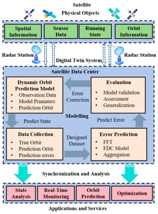
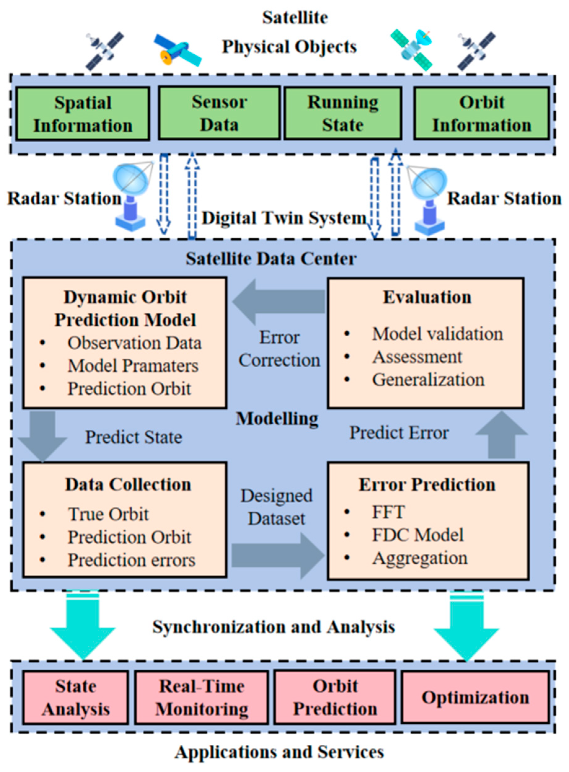
The proposed satellite orbit prediction digital twin system is shown in Figure 1, which consists of three parts: the physical entity layer, the digital twin system layer, and the application layer [13]. The specific functions and interaction logic of these modules are described as follows:
Figure 1.
Digital twin system for orbit prediction.
Physical entity layer: This layer comprises the physical satellite and ground-based radar stations. The satellite generates real-time sensor data and running state information, while the radar stations track the satellite to provide precise observational data. This layer serves as the data source for the entire system.
Digital twin system layer: This is the core processing unit, primarily housed within the Satellite Data Center. It operates through a closed-loop interaction logic involving three key steps:
Data collection: Raw data from the physical layer is aggregated to form a “Designed Dataset,” which includes true orbit data and initial prediction errors. Specifically, ILRS data is used as the real orbit in this article
Modelling: This module contains two parallel but interactive models. First, the Dynamic Orbit Prediction Model calculates the theoretical orbit based on orbital mechanics. Simultaneously, the Error Prediction Model (the proposed FDC model) utilizes FFT and deep learning to predict the residual errors generated by the dynamic model.
Evaluation: The predicted errors are fed back to correct the dynamic model’s output. The system then evaluates the accuracy and generalization of the correction to ensure reliability.
Application layer: Based on the high-precision orbit determination from the twin layer, this layer provides downstream services, including real-time state analysis, orbit monitoring, and optimization strategies for satellite operations.
3.2. Problem Formulation
The orbit obtained through the dynamic prediction model is defined as the state vector where t represents the timestamp. At a specific timestamp t, the predicted state is denoted as: . The predicted values in different dimensions represent the position and velocity variables of the satellite in three directions of the earth-centered earth-fixed (ECEF) coordinate system, respectively. Similarly, the real satellite orbit data is denoted as . At specific timestamp t, . The error vector obtained by subtracting the true orbit data from the dynamic orbit prediction value is . Selecting a time window length L and backtrack from time k to obtain an error sequence as initial error where . Selecting another time u to backtrack the time window L and obtain another error sequence as predict error . The purpose of prediction is to find a map relationship that maps . In this article, this function is applied as an FDC model, and its specific implementation principle will be detailed in the following subsections.
3.3. Methodology
In previous studies, we identified the shortcomings of the STL-TCN model [13]. When orbit data with intervals exceeding one month is used as the testing dataset, the performance of the model will significantly decrease. Specifically, once the prediction horizon extends beyond one month, the STL-TCN model exhibits a rapid escalation in MAE, surpassing the threshold of 1. This corresponds to a positional deviation in the kilometer range, rendering the model inadequate for high-precision applications such as satellite collision avoidance. The reason for this result may be that the features learned by the time series prediction model have strong temporal correlation, and it is expected that the performance of the model will decline as the time interval increases. To address this issue, we employ a frequency-domain analysis method. Unlike time-domain models that rely on sequential dependencies, the frequency-domain approach transforms the signal into spectral components, capturing the global and stable periodic patterns of the orbit errors. This allows the model to learn invariant features that are less affected by the length of the time interval. This approach consists of two steps: frequency-domain transformation and frequency derivation.
The orbit error signal is transferred from the time domain to the frequency domain through the Fourier transformation. Specifically, using the given time-domain error signal , , which is expressed in scalar form as the orbital error vector . The parameter T satisfies condition , where n denotes the number of sampling points within the sliding window. Consequently, the frequency integration is confined to the effective bandwidth , representing the finite spectral components captured from the orbit data. We convert it into a frequency-domain signal by following equation:
After completing the frequency domain conversion, we decompose the frequency signal into multiple components and export them separately for prediction. Thus, we referred to the approach in reference [14]. The entire spectrum for the signal is used to derivate a representation of the time signal in the reconstructed time domain. The specific method is to decompose the spectrum into multiple orders of information by designing a Fourier derivative operator to improve accuracy. We define this operation as Fourier derivative transformation (FDT). The design of the Fourier derivative operator is as follows
where represents the m-order Fourier derivative operator. The inverse transformation can be defined as
Then, we employed a bank of three parallel filters to process the signal components simultaneously. The three filters are designed to decompose the signal into intermediate frequency (IF), low frequency (LF), and high frequency (HF) components. We utilized Butterworth filters for their flat passband characteristics.
The filtered components are input into a Fourier dilated convolutional network for regression. This architecture utilizes Fourier convolution to reduce computational cost by transforming convolution into element-wise multiplication. Simultaneously, dilated convolution expands the receptive field, enabling the model to effectively capture information from the full frequency spectrum of the components.
The idea of Fourier convolutional networks originates from the classical Fourier convolution theorem: convolution in the time domain is equivalent to point wise multiplication in the frequency domain. This property is cleverly introduced into neural network design to improve computational efficiency and enhance the global modeling capabilities. Define two continuous time signals and ; the convolution between them can be written as
If we define the Fourier transform of two signals as and , we can get
This frequency-domain multiplication strategy greatly improves computational efficiency. It reduces the convolution operation with complexity to by using Fourier transform.
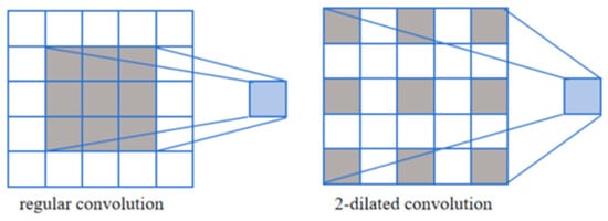
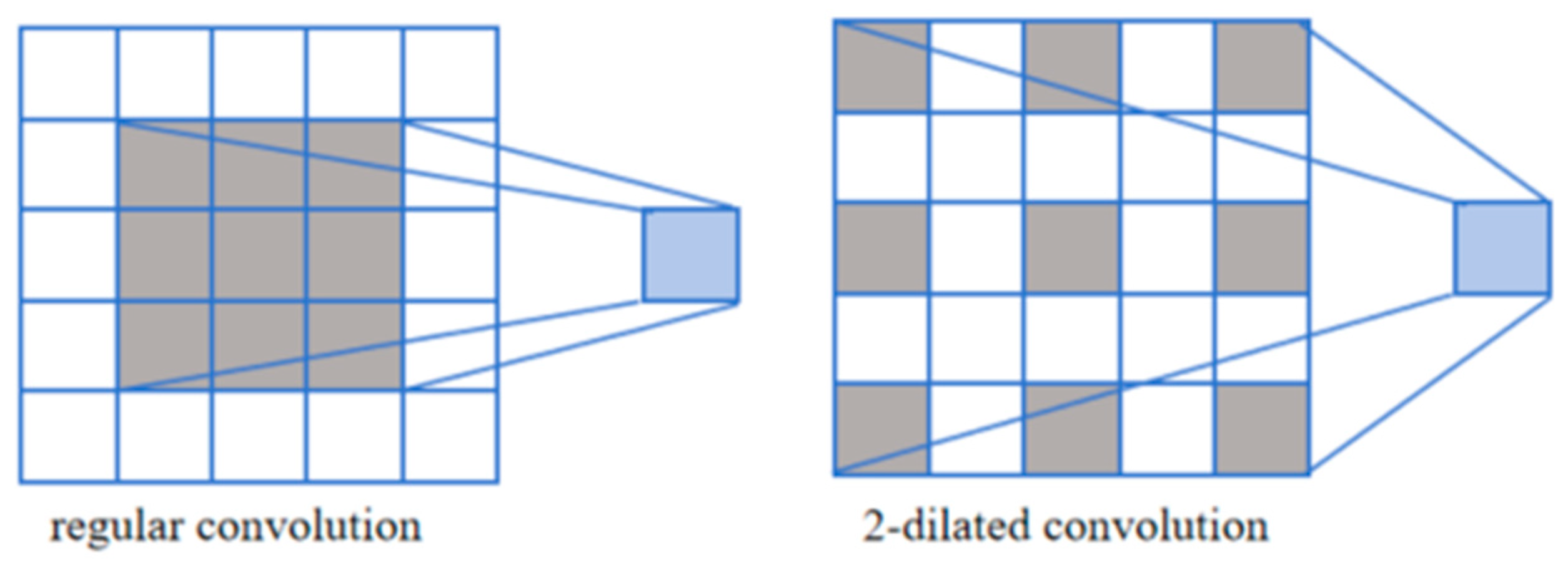
The dilated convolution is illustrated as follows. Dilated convolution originated in the field of image segmentation [25]. The pooling operation in Fully Convolutional Networks (FCN) reduces the receptive field of the network, which results in information loss. To address this limitation, dilated convolution has been proposed. Its original design intention was to enable the network to gain a larger receptive field without pooling.
Figure 2 shows a comparison between the regular convolution and the two-dilated convolution. Dilated convolution introduces a dilation coefficient . The value of determines the interval between the elements participating in the convolution. As shown on the right side of Figure 2, when , the interval between each element participating in the convolution is 1. Its original design enables the network to gain a larger receptive field without pooling.
Figure 2.
Comparison between regular convolution and dilated convolution. The gray squares represent the active pixels involved in the convolution operation, while the white squares are inactive.
The integration of FDT and the convolutional network is realized through a three-stage mechanism: decomposition, adaptive mapping, and reconstruction. First, the FDT decomposes the input into m derivative components. Second, the order m of the FDT directly modulates the dilation rate and depth of the subsequent convolutional layers, creating an ’adaptive receptive field.’ Finally, the inverse FDT acts as a physical regularizer during the output reconstruction phase.
4. Fourier Dilated Convolutional Prediction Model
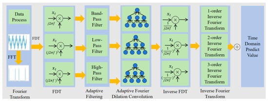
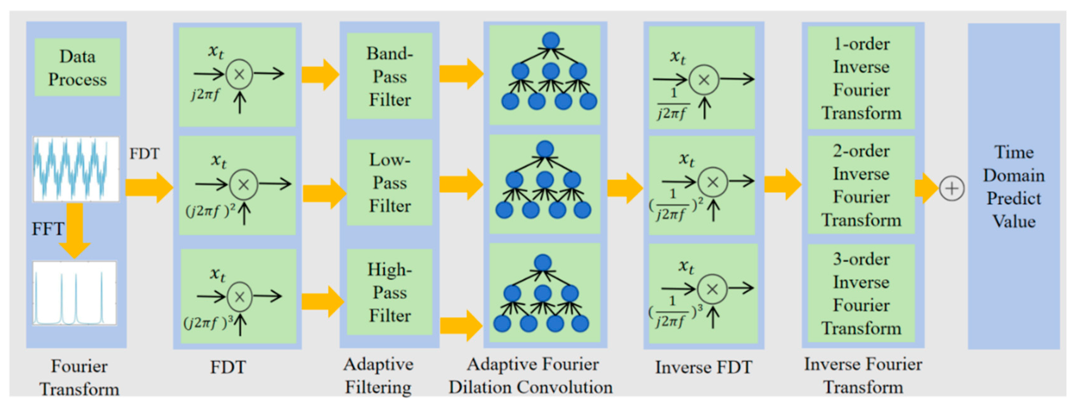
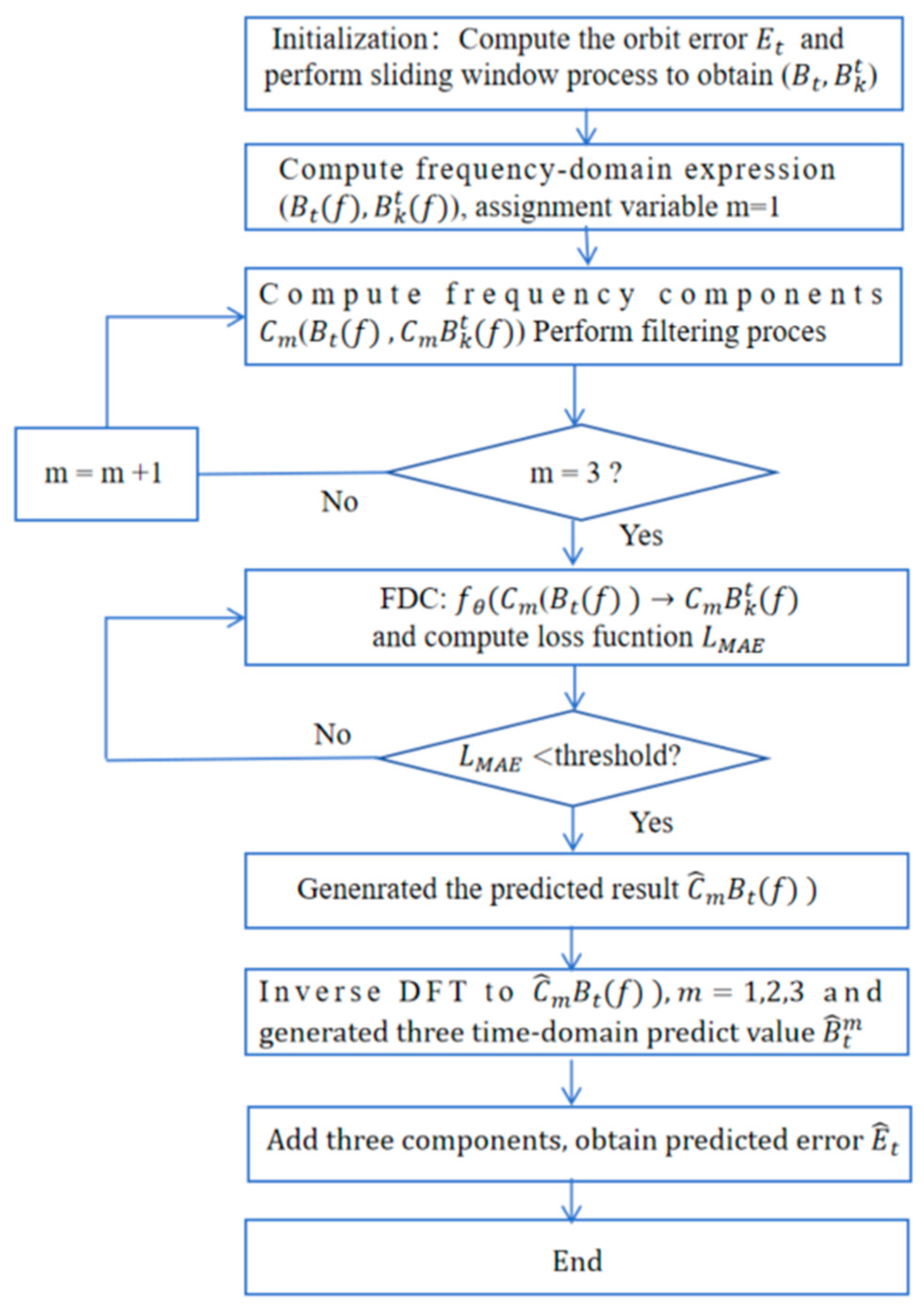
Generally, previous predictions cannot satisfy the high demand of the integrated space–air–ground network [7]. The specific process of the FDC model is shown in Figure 3. Firstly, the satellite orbit transformation data arranged in chronological order will be preprocessed as a time-series signal. We transform time-domain signals into frequency-domain signals through Fourier transform. In the next steps, the frequency domain data is decomposed into three frequency-domain components through FDT. Then, we perform dilated Fourier convolution for the different components separately. According to the definition of the Fourier transform, the convolution of a signal in the time domain can be transformed into a product in the frequency-domain. Therefore, for frequency domain data, this approach greatly reduces computational complexity. In addition, the introduction of dilated convolution allows the entire model to perceive a larger frequency domain range compared to a traditional convolution network such as CNN. The frequency domain convolution results are subjected to inverse Fourier derivative transformation and inverse Fourier transform to convert the frequency domain prediction results back to the time domain. Finally, three components in the time domain are added to obtain the final satellite orbit prediction results. The Fourier derivative transformation and dilated convolution will be explained in detail in the following content.
Figure 3.
The workflow of the Fourier dilation convolution model.
4.1. Data Preprocess
In this section, we briefly explain the process of data preprocessing. We used two real satellite orbit datasets, TLE and ILRS. The Two-line element is a standard format used to describe the orbit parameters of a satellite. It consists of two lines of text, containing all the key information required for satellite orbit, allowing users to calculate the position and velocity of the satellite at any given time. The first line usually contains information such as the satellite number, NORAD Catalog Number, launch year, orbit type, etc. The second line contains the orbital parameters of the satellite, such as the semi major axis, eccentricity, inclination, right ascension, and perigee angle [10]. We set the sampling interval for TLE data to 3 min, while the sampling interval for ILRS data is given by NASA, usually 3’5 min. In this article, we collected publicly available TLE datasets and generated TLE orbit data using the SGP4 dynamic model [6].
International Laser Ranging Service was established in 1998 with the aim of organizing and coordinating global satellite laser ranging (SLR) and lunar laser ranging (LLR) activities [11]. In this article, we use ILRS data as the real data of satellite orbit. The satellite orbit error E is calculated using the following equation
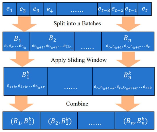
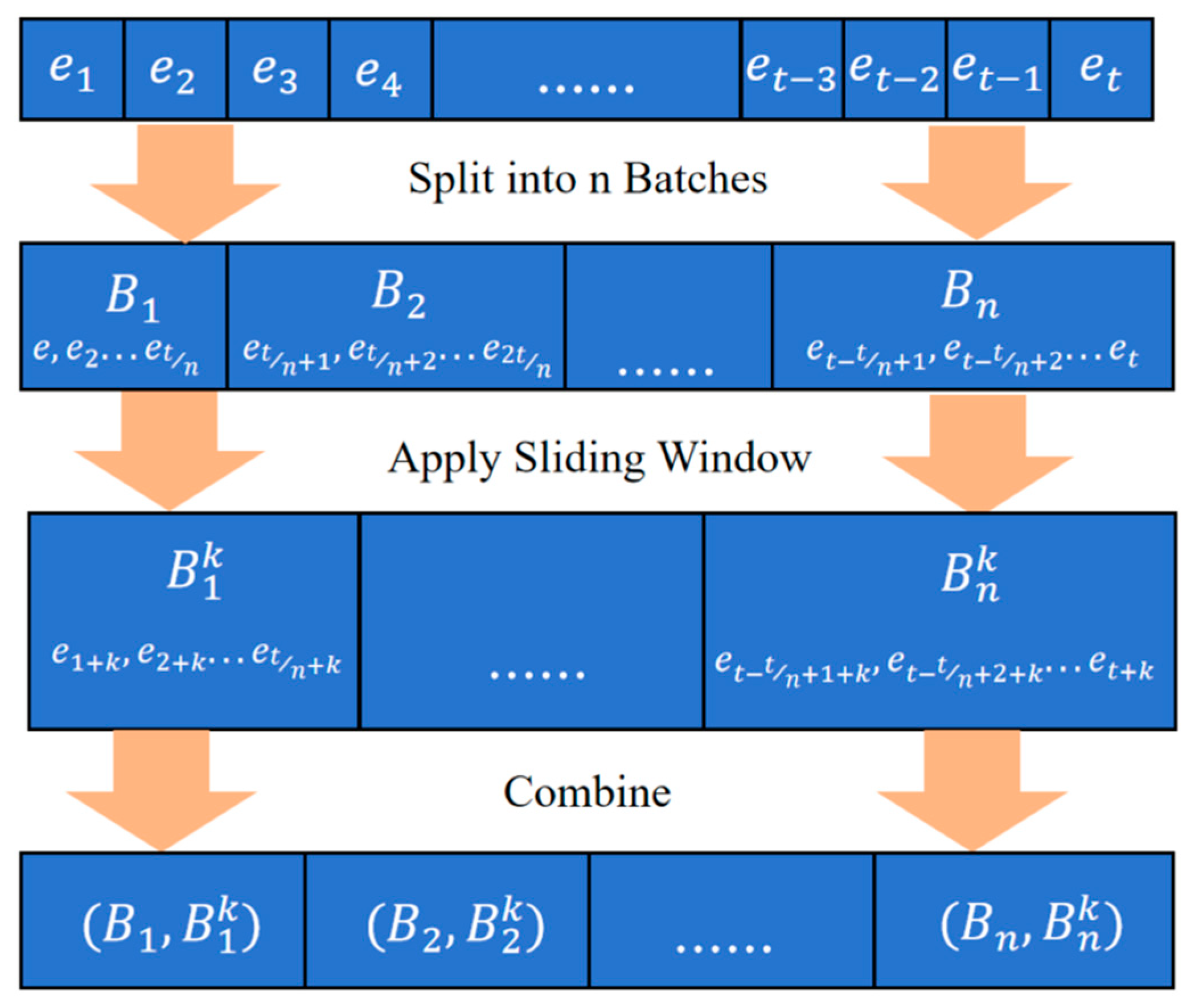
Assuming a known sequence of orbital errors . We use the sliding window method to divide sequence into some batches for training. The process is shown in Figure 4. Firstly, sequence is divided into n batches to get sequence , in which . Each batch slides forward k timestamps through the time window to obtain a sequence , where and . We use zero-padding to complete the excess parts that move forward in the batch. Then, we pair the original sequence with the sequence processed using a sliding window to obtain . Our goal is to find a mapping relationship that satisfies
Figure 4.
Sliding window processing procedure.
4.2. Three-Order Decomposition
According to the description of the FDC workflow in the previous subsection, perform FFT on sequence according to Equation (1) to obtain the frequency-domain expression of the orbit error data . Next, according to Equation (2), use the Fourier-derivative operator to decompose the frequency-domain representation of each batch into three frequency components which can be expressed as
where represents the order and ]. The selection of these three specific orders (1, 2, 3) and their corresponding frequency ranges is theoretically grounded in the properties of the Fourier derivative transform and orbital perturbation characteristics. The 1st-order term corresponds to the periodic perturbation error (e.g., atmospheric drag). In the frequency domain, periodic variations manifest as energy concentrated in the mid–low frequency band, synchronized with the orbital period. The 2nd-order term corresponds to the trend/acceleration residual (e.g., Earth’s non-spherical gravity). These long-term cumulative effects, such as secular perturbations, appear as low frequency components in the spectrum. The 3rd-order term captures the abrupt/jerk errors (e.g., geomagnetic storms). These impulsive disturbances contain rich high-frequency information, falling into the high frequency band [26].
Then, we filter the three components based on the spectrum of orbital error. The filtering process can be considered feature enhancement of the main physical meanings of the components. Filter out the unimportant frequency domain parts in each component through the filtering process, while retaining the frequency-domain energy caused by orbital perturbation, unmodeled residuals, or sudden disturbances. The physical meanings of the three components are explained as follows:
- The first-order component corresponds to periodic perturbation error, with a characteristic frequency of mid to low frequency. Therefore, we use a bandpass filter for filtering.
- The second-order component corresponds to the acceleration residual generated by perturbation forces that are not included in the dynamic model, with a characteristic frequency of low frequency. Therefore, we use a low-pass filter for filtering.
- The third-order components correspond to sudden perturbation errors, and the characteristic frequency range is high frequency. Therefore, we use high pass filtering for filtering.
Based on the analysis of the orbital dynamics, we designed three filters to process three components to preserve their main frequency domain features. The parameters design of the three filter is shown in Table 1.
Table 1.
Parameters of the 3 filters.
4.3. Three-Order Dilated Convolution
The prediction process is completed through Fourier dilated convolution. In this article, we designed a 3-order Fourier dilation convolution based on the physical meanings of three frequency-domain components. The specific parameters are shown in Table 2.
Table 2.
Parameters of adaptive dilated convolution.
Specifically, the first-order component corresponds to periodic perturbation factors such as atmospheric drag, solar and lunar gravity. Therefore, the dilation convolution rate should be selected as moderate to capture periodic fluctuation features. The size of the convolution kernel is , and the convolution layer size is set to 3, corresponding to the selection of a medium convolution size in our qualitative analysis. The activation function is chosen as Relu to capture periodic fluctuations.
The acceleration corresponding to the second-order sub model reflects the orbital error, which is related to trend perturbation factors such as the non-spherical gravity of the Earth and long-term changes in atmospheric density. These types of perturbation forces typically have a period of several months or years; therefore, high expansion rates and deeper convolution layers should be selected to capture long-term trend features. The size of the convolution kernel is , and the convolution layers are set to 5, corresponding to the qualitative analysis of long-range feature capture and deep convolution layer analysis. The activation function is selected as Relu to capture trend fluctuations.
The third-order component reflects the degree of sudden change in error, which is related to sudden space weather events such as solar flares and geomagnetic storms. Therefore, a low dilation rate and shallow convolution layers are chosen to capture abrupt pulse features. The size of the convolution kernel is , and the convolution layers are set to 5, corresponding to the qualitative analysis of long-distance feature capture and deep convolution layer analysis. The activation function is selected as Sigmoid to capture abrupt features in the frequency domain and preserve more details.
The convolution prediction result of frequency domain components is defined as . The purpose of convolution is to make close to , which can be expressed as
We control the convergence process of the convolutional network through the mean absolute error (MAE) as the loss function. It can be defined as
where is the number of samples, is the loss function and is the number of data in sequence.
After the convolutional model reaches convergence, we perform inverse FDT on the prediction results . Firstly, according to Equation (4), we perform inverse derivate transformation on the frequency domain components as follows
where is defined as inverse derivative transformation of frequency domain component prediction results. Then, we perform inverse Fourier transform for by Equation (2) to obtain the time-domain expression of each predicted frequency component which can be expressed as
where is defined as the time-domain expression of each predicted frequency component. Finally, we add up the time-domain components of each prediction and extract the repeated parts in the sliding window to obtain the final prediction result .
4.4. Algorithm and Evaluation
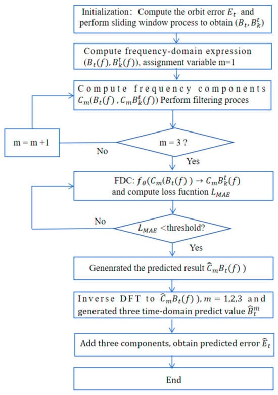
The complete process of orbit prediction by the FDC model is summarized in Figure 5. To evaluate the performance of FDC prediction error, we applied three metrics: MAE, RMSE, and . Their calculation methods are as follows.
where is the amount of data in sequence and is the average of the real value. Generally, smaller values of MAE and RMSE indicate better model performance, while larger values indicate poorer model performance. the value range of is . The closer the value is to 1, the better the performance of the model; the farther the value is from 1, the worse the performance of the model.
Figure 5.
Block diagram of FDC algorithm.
Furthermore, to analyze the interpretability of the FDC model, we applied SHAP values. The main idea of SHAP value comes from cooperative game theory, which is a method of evaluating player contributions and distributing profits [15]. In machine learning, SHAP values are used to explain the contribution of each feature value of a learning model to the predicted output for a certain input state. Assuming an n-dimensional space and a set S satisfy and , then S is defined as the union of features . The SHAP value of is defined as the weighted sum of contributions from all possible unions, which is computed by following
where is defined as the SHAP value, is defined as the prediction value of S and is the total number of features. In this paper, SHAP value is used to measure the ‘marginal contribution’ of the three frequency-domain components to the output of the FDC model and output as expected value. Hence, the range of SHAP value is defined as .
5. Experiment Results
In this section, we conducted extensive experiments to validate the proposed FDC model. Firstly, a simulation operating environment for satellite orbit was constructed using STK 11.6 software. The effectiveness of the proposed model was validated using two satellite datasets, TLE and ILRS. Then, the performance of the FDC model was compared with various models in existing research. Finally, the generalization ability of the FDC model was verified using five real satellites and orbit data at different times.
5.1. Simulation Environment
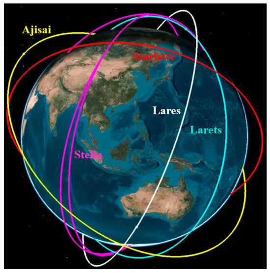
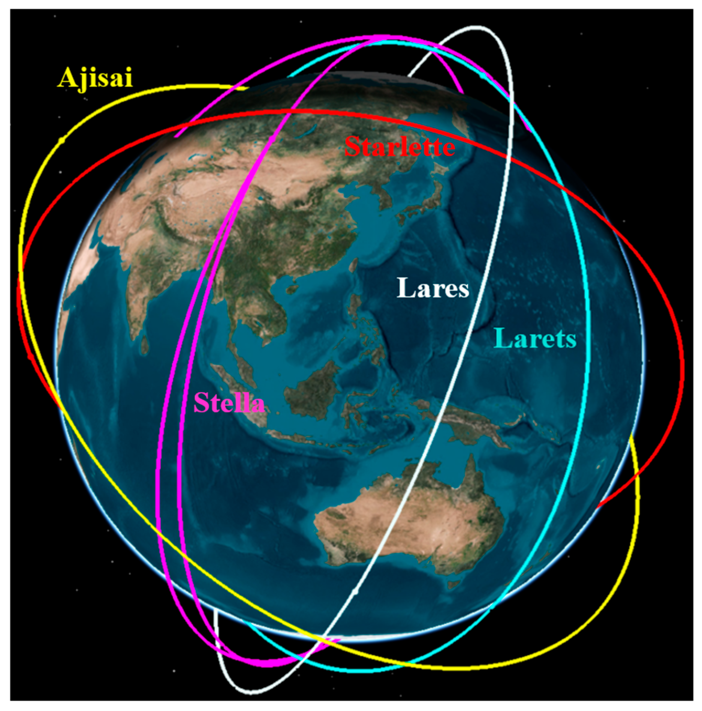
As shown in Figure 6, we use publicly available TLE data from five real satellites in the experiment and construct a simulation environment using STK 11.6 software. The curves of different colors in the figure represent the TLE orbits of different satellites. The yellow curve represents satellite Ajisai, the white curve represents satellite Lares, the green curve represents satellite Larets, the red curve represents satellite Starlette, and the purple curve represents satellite Stella. More detailed data on these five satellites are shown in Table 3 which lists the NORAD ID, orbit type, launch year, period, perigee and apogee of the five satellites, respectively.
Figure 6.
Satellite simulation experiment scene constructed by STK.
Table 3.
Parameters of 5 satellites.
As mentioned earlier, the accuracy of satellite orbit data generated through TLE data and SGP4 model is not high. Therefore, another high-precision dataset ILRS was adopted to calculate the orbit error.
5.2. Effectiveness Assessment
To verify the effectiveness of the FDC model, we choose orbit data from the satellite Stella. The training dataset contains a total of 174,720 entries, covering 1 year’s orbit data from satellite Stella (2 January 2022–31 December 2022) and the testing dataset contains a total of 14,780 entries, covering about 1 month’s orbit data (1 January 2023–31 January 2023). The sampling interval is set to 3 min. Each piece of data has six dimensions and represents the position and velocity of the satellite in the X, Y, Z directions in the geocentric coordinate system. Each batch contains 256 pieces of data, with a total of 683 batches and setting . Long-distance time series prediction is achieved through multi-step iterative prediction, which uses the predicted output of the previous step as the input for the next prediction.
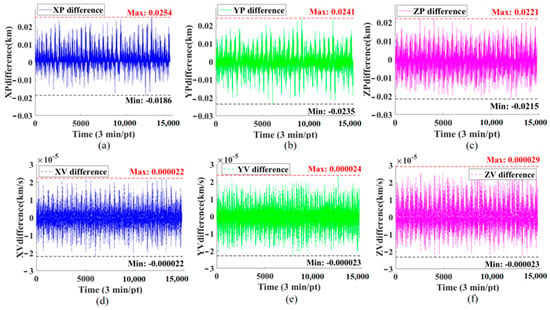
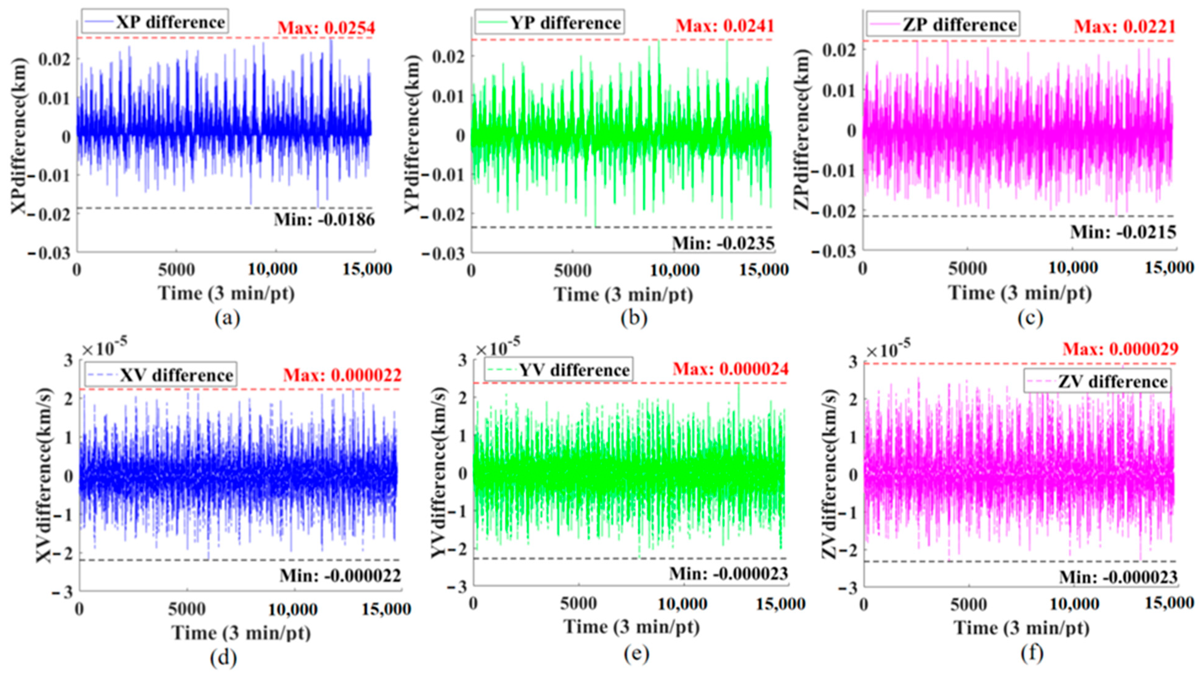
The performance of the FDC model on the testing dataset is shown in Figure 7. Figure 7a–c represents the performance of the model on the position variable, and Figure 7d–f represents the performance of the graph on the velocity variable. The horizontal axis represents the timestamp, and the vertical axis represents the difference between the FDC model’s predicted error value and the true error value. From Figure 7, it can be observed that the prediction difference value of the FDC model in the position variable mostly does not exceed 0.0254 km, and the error in the velocity variable does not exceed km/s. This proves the effectiveness of our proposed FDC model, which can achieve high-precision prediction results (position error < 25.4 m), significantly outperforming standard coarse orbit data (TLE data).
Figure 7.
Difference between real orbit error and FDC prediction error. (a) The difference in X-position; (b) The difference in Y-position; (c) The difference in Z-position; (d) The difference in X-velocity; (e) The difference in Y-velocity; (f) The difference in Z-velocity.
Furthermore, in order to compare the performance of the proposed FDC model with the AI models proposed in existing research, we also used the same dataset from the Stella satellite to calculate the MAE values of each model after convergence. To ensure a fair and rigorous comparison, the training conditions and hyperparameters for all models were carefully configured. As detailed in Table 4, all models, including the proposed FDC and the six benchmark models (STL-TCN [9], TCN [8], LSTM, SVM [10], ANN [14], and CNN), were trained on the same dataset partitions with identical batch sizes, optimization algorithms (Adam), and initial learning rates. Regarding the specific structural parameters, the decomposition order of the proposed FDC model was set to three to balance computational complexity and feature extraction capability. For the comparison models, the key hyperparameters, such as the kernel size and dilation factors for the TCN-based models, the number of hidden units for LSTM, and the regularization parameters for SVM—were determined via grid search or referenced from the established literature to ensure they operated at their optimal performance levels. This unified experimental setup guarantees that the performance differences observed in the results are attributable to the models’ architectures rather than discrepancies in the training configurations.
Table 4.
Parameter settings and training conditions for the FDC and comparison models.
Based on the standardized parameter settings and training protocols described above, we conducted extensive experiments to evaluate the predictive performance of the proposed FDC model against the six baseline models. Table 5 presents the detailed comparison of the MAE for both position and velocity components across all satellite datasets. These quantitative results demonstrate the superiority of the FDC model, particularly in handling long-sequence orbital predictions, and provide a basis for the subsequent analysis of its error distribution characteristics.
Table 5.
Comparison of MAE value of FDC model with 6 ML models.
It can be observed from Table 5 that the FDC model performs slightly better in predicting position variables than velocity variables. Position and velocity prediction performance differ primarily due to the dimensional scale discrepancy: the larger magnitude of positional values () dominates the loss function gradient, resulting in higher relative accuracy for position compared to velocity ().
In terms of comparative analysis, the FDC model demonstrates competitive performance relative to the STL-TCN model, while STL-TCN shows marginal advantages in and due to its specialized decomposition of trend components. Compared to traditional LSTM, SVM, ANN, and CNN models, the FDC model has an MAE value that is approximately one order of magnitude smaller. This result can be encountered, as traditional neural network models often suffer from overfitting or underfitting when dealing with long sequences, and may fall into local optima during training, leading to convergence difficulties. However, the dataset in this article is relatively large (174,720 entries) and not friendly to these models.
In addition, we evaluated the inference latency using an input sequence length of 1478 on an Intel Core i5-8500 CPU. The proposed FDC model, leveraging the efficiency of the FFT, achieves an estimated inference time of approximately 0.5 ms to 0.6 ms. In contrast to a traditional machine learning model like LSTM, TCN typically require 4 ms to 15 ms due to heavy matrix multiplications. These empirical results demonstrate that the FDC model is faster by an order of magnitude than its deep learning counterparts. Given the significantly reduced execution time and parameter count (on the order of hundreds), the proposed FDC model demonstrates superior energy efficiency, consuming approximately one order of magnitude less energy per inference compared to recurrent neural networks.
5.3. Robustness Assessment
In this subsection, to further validate the robustness of the FDC model, we apply different noise influences to evaluate their impact on performance, and then used orbit data from different satellites as the test set to evaluate the performance of the model.
According to the analysis of orbital dynamics, the satellite orbit is not only affected by the three-body perturbation force, but also by atmospheric density. Although the atmospheric density perturbation force is much smaller than the Earth’s gravity, long-term effects can also cause satellite orbits to deviate. We add atmospheric density perturbation as noise disturbance to the orbital data to modify the test set, and then use the modified dataset to test the trained FDC model to evaluate its robustness. Ding Yigao et al. [27] reviewed multiple atmospheric density models. In this study, we used these eight models to introduce density perturbations. The atmospheric drag perturbation is introduced as a noise disturbance. The acceleration due to atmospheric drag is modeled as
where represents the mass density of the Earth’s atmosphere at the satellite’s altitude, represents the dimensionless parameter that characterizes the satellite’s geometric shape and its interaction with the atmospheric flow, represents the projected area of the satellite perpendicular to the velocity vector, represents the total mass of the satellite, represents the magnitude of the satellite’s velocity relative to co-rotation, represents the relative velocity vector. We applied these eight models and calculated their MAE values for comparison. The specific results are shown in Table 6.
Table 6.
MAE value of eight atmospheric density models.
Table 6 presents the MAE values of the FDC model prediction results corrected by eight atmospheric density models. Generally, the introduction of these models results in a slight increase in MAE values compared to the initial data, yet the magnitude of deviation varies. The DTM2000 model demonstrates the highest overall stability, exhibiting MAE values closest to the initial data across the majority of variables, particularly showing negligible deviation in the velocity variable . The J71 model also performs well in position variables and , closely matching the initial values, but exhibits a notable deviation in the variable. In contrast, the JB2006 model induces the most significant error increase, especially in position variables, while models like DTM78 and NRLMSISE00 show intermediate levels of impact. Overall, DTM2000 proves to be the most robust model with the least interference to the baseline prediction accuracy.
5.4. Distribution Offset Assessment
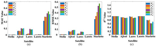
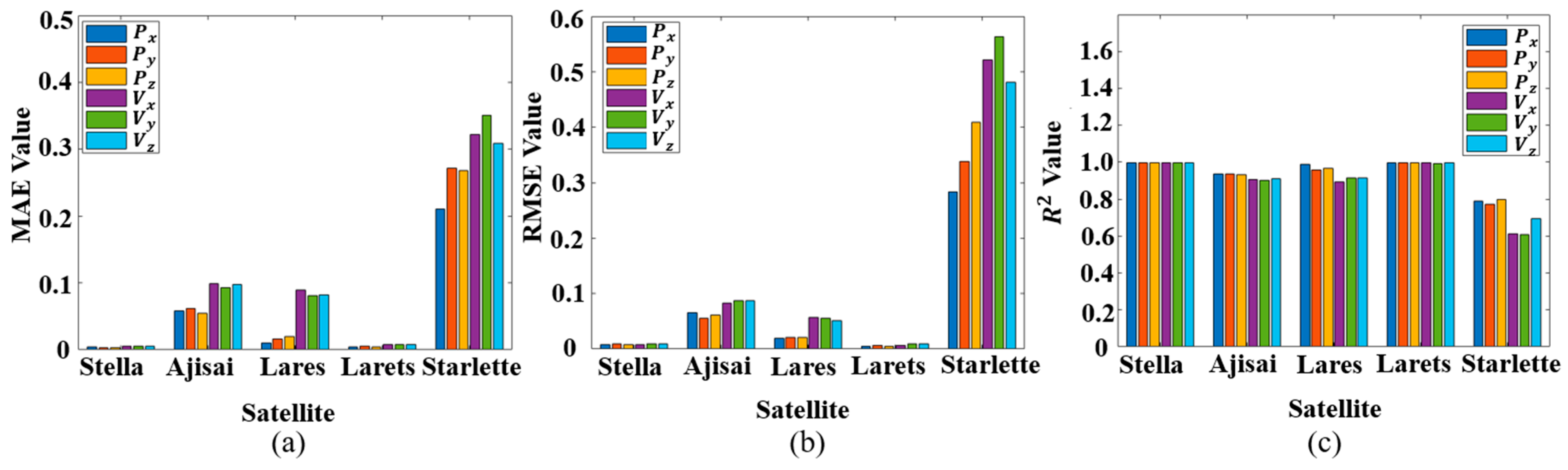
In addition, the Stella satellite is a sun-synchronous orbit (SSO) satellite. In order to verify its predictive performance for other orbit types of satellites, we used the orbit errors of four other satellites for one month as the test set to predict the FDC model. The predicted evaluation results were evaluated using three indicators: MAE, RMSE, and . The evaluation results are shown in Figure 8.
Figure 8.
Performance evaluation of FDC model prediction in different satellite orbits. (a) The MAE of the FDC model for five satellites; (b) The RMSE of the FDC model for five satellites; (c) The of the FDC model for five satellites.
Figure 8a–c represents the MAE, RMSE, and metrics respectively. The horizontal axis represents satellites, and the vertical axis represents indicator values. Each cluster of columns contains six columns representing the position and velocity variables of the satellite. The horizontal axis represents the different satellites, and each cluster of bars corresponds to the position (, , ) and velocity () variables
It is observed that the FDC model achieves optimal performance on the Lares and Stella satellites, exhibiting the lowest errors and highest values. This superior performance is attributed to their near-circular orbits and stable orbital dynamics, which present consistent frequency domain characteristics that are easily captured by the FDC model.
In contrast, the prediction performance for Ajisai shows a slight degradation. This is likely due to its distinct physical properties, specifically its high Area-to-Mass Ratio (AMR) as a geodetic sphere, which makes it more susceptible to solar radiation pressure, introducing complex non-gravitational perturbations.
The model exhibits the largest prediction errors on the Starlette satellite. This result is primarily driven by Starlette’s higher orbital eccentricity and lower perigee altitude compared to the others. These factors result in significant periodic velocity variations and stronger atmospheric drag perturbations, creating high-frequency non-linearities that are more challenging for the model to fit.
Despite these variations, the FDC model demonstrates strong robustness. While performance fluctuates based on orbital complexity, the model maintains high accuracy across the majority of the tested satellites, validating its effectiveness in handling diverse orbital regimes.
In our previous research [9], we found that the STL-TCN model has weak generalization ability for future data. When the time interval between the test set and the training set exceeds one month, the prediction accuracy of the STL-TCN model will greatly decrease, making it unsuitable for engineering applications. Therefore, we came up with the method of prediction through frequency domain analysis, due to the weak temporal correlation of satellite orbit frequencies.
In this subsection, in order to verify the anti-interference ability of the FDC model for time distribution offset, we collected orbit data of a Stella satellite every other week. The test dataset also covered the orbit information of the satellite within one week, sampled every three minutes. Each test set had a total of 3360 data points, and the MAE, RMSE, and metrics were calculated for each prediction. The performance evaluation of the FDC model is shown in Figure 8.
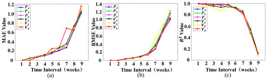
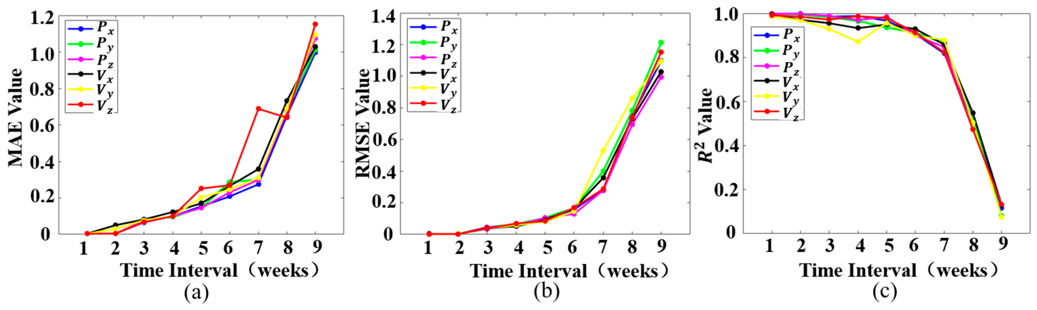
Figure 9a–c represents the changes in MAE, RMSE, and values at different time scales, respectively. The horizontal axis represents the time interval between the testing dataset and the training dataset, with each scale representing 1 week. Blue, green, and purple represent position variables in the X, Y, and Z directions, respectively, while black, yellow, and red represent velocity variables in the X, Y, and Z directions, respectively.
Figure 9.
Performance evaluation of FDC model prediction in different time scales. (a) The evolution of MAE for the FDC model over a 9-week period; (b) The evolution of RMSE for the FDC model over a 9-week period; (c) The evolution of for the FDC model over a 9-week period.
The overall trend in Figure 8 shows that as the time interval increases, the performance of the model continues to decline. But the model performs well on data with intervals of 1–7 weeks. On the dataset with an 8-week interval, the MAE and RMSE values suddenly increased, while the value suddenly decreased. This result illustrates that the validity period of the model is approximately in the 6-th/7-th week.
Table 7 presents a quantitative comparison of the validity periods between the FDC and STL-TCN models based on specific MAE failure thresholds. While the STL-TCN model maintains validity for approximately 15–19 days, the proposed FDC model significantly extends this duration to 42 days across all six orbital variables.
Table 7.
MAE comparison at the point of failure between FDC and STL-TCN.
Specifically, the ‘MAE at Failure’ columns demonstrate the point where the prediction exceeds the defined thresholds ( for position and for velocity). The FDC model’s errors are tightly clustered around these limits. This confirms that the FDC model effectively utilizes the error budget, providing a precise definition of its validity period and demonstrating superior long-term stability compared to the STL-TCN model.
5.5. Interpretability Analysis
In order to better reveal the inherent laws of the FDC model, a SHAP analysis method was adopted to analyze the impact of the three frequency-domain components on the performance of the FDC model.
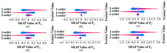
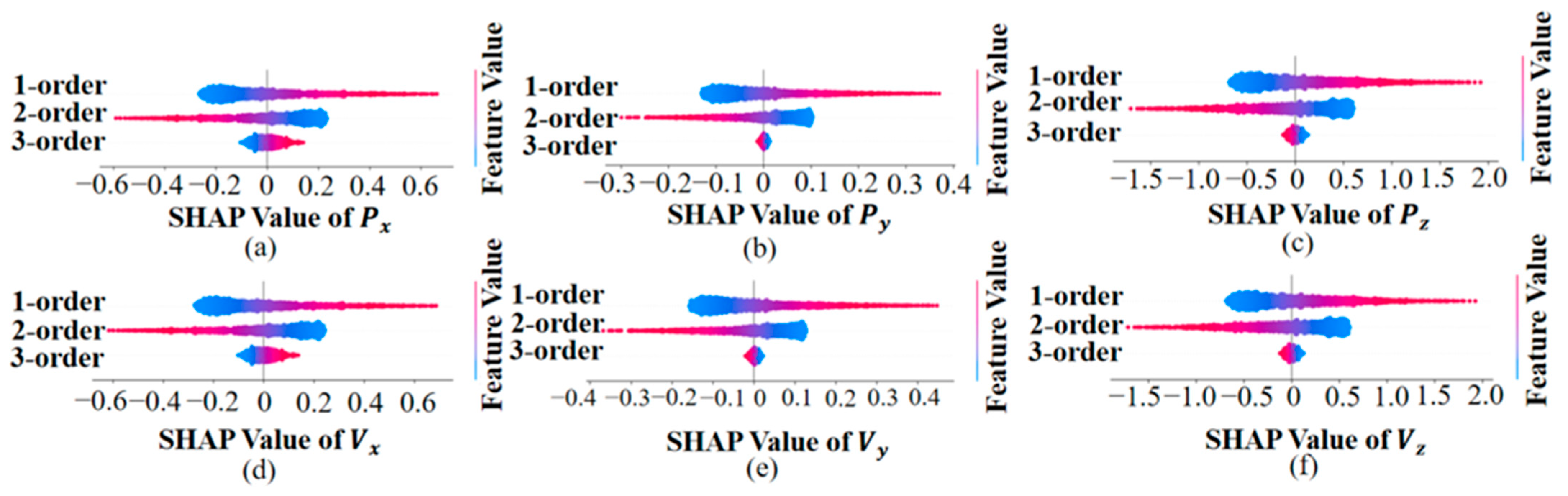
Figure 10 shows the SHAP analysis of the 3-order frequency-domain variables. Figure 10a–c represents the SHAP values of the FDC model on the position variable, and Figure 10d–f represents the SHAP values of the FDC model on the velocity variable. In each subgraph, the scattered clusters from top to bottom represent the 1-order, 2-order, and 3-order frequency components, with the horizontal axis representing the SHAP values and the vertical axis representing the feature values.
Figure 10.
The SHAP analysis result of the FDC model for the three frequency components in Stella. (a–c) represent the SHAP values for the position variables (), and (d–f) represent the SHAP values for the velocity variables ().
To provide a quantitative perspective, we analyzed the distribution range of the SHAP values for each component. As shown in the subgraphs, the 1st-order and 2nd-order components exhibit significantly wider distributions (spanning roughly from −0.4 to 0.4 and −0.2 to 0.2, respectively) compared to the 3rd-order component, which is tightly clustered around zero. This indicates that the 1st-order and 2nd-order components contribute approximately 50% and 40% to the model’s output, respectively, while the contribution of the 3rd-order component is marginal (less than 10%).
From the perspective of orbital dynamics, the 1-order component reflects the rate of change of error and is directly related to periodic perturbations such as atmospheric drag, solar and lunar gravity, and solar pressure. The characteristic period of this type of perturbation is consistent with the satellite orbit period, corresponding to the mid to low frequency range of the frequency domain. The 2-order component represents the acceleration modulation caused by periodic or quasi periodic perturbations in orbital dynamics, reflecting the residuals of unmodeled perturbations at the acceleration level. It is mainly caused by the long-term cumulative effects of such errors caused by periodic or quasi periodic perturbations (such as Earth’s oblateness and solar and lunar gravity), corresponding to the low-frequency range of the frequency domain.
The 1-order and 2-order components constitute the main energy component of orbit error, so accurate prediction of these two components has a significant impact on the prediction accuracy of orbit error. In other words, they have the greatest marginal contribution to orbit error prediction.
The 3-order component reflects the degree of sudden change in error and is related to noise or residuals in the dynamic model. This type of perturbation has randomness and wideband characteristics, corresponding to the high-frequency band of the frequency domain. In the frequency domain, this part of the error usually appears in the form of high-frequency noise. On the one hand, the proportion of such errors in the frequency domain expression of orbital errors is much smaller than the periodic and unmodeled perturbation forces represented by the first-order and second-order components, respectively; on the other hand, the sampling interval of the ILRS public datasets is usually 3–5 min, and this low-frequency sampling makes it difficult to capture significant high-frequency noise. Therefore, this results in the minimum marginal contribution of the third-order components to the FDC model.
6. Conclusions
This study addresses LEO satellite orbit prediction by regarding orbit data as a time-series signal and applying signal analysis and processing techniques.
In this paper, we propose a novel frequency-domain analysis paradigm for orbit error prediction, building upon the findings of existing research. First, Fast Fourier Transform (FFT) is used to transform orbital data from the time domain into the frequency domain, producing the corresponding spectrum. Then, the workflow and modeling process of the proposed FDC model are elaborated, in which a third-order adaptive Fourier derivative transform is adopted to decompose the frequency-domain signal into three distinct components. A dilated convolutional network is then applied to conduct regression prediction on each component separately. Finally, inverse Fourier differentiation and inverse Fourier transform are used to reconstruct the predicted time-domain orbital values by combining the estimated frequency components, generating the final orbit prediction result. Additionally, the effectiveness of the FDC model is verified via simulation experiments as well as two real datasets. Specifically, the FDC model maintains the MAE in satellite Stella for position components consistently around km/s and for velocity components around km/s. Furthermore, the experimental results demonstrate that the model exhibits favorable robustness and strong resilience against distribution shifts.
Author Contributions
Conceptualization, X.X., H.W. and W.H.; methodology, X.X., H.W. and W.H.; software, X.X. and W.H.; validation, H.W.; formal analysis, L.C.; investigation, Y.Z.; writing—original draft preparation, X.X., L.C., Y.Z. and T.L.; writing—review and editing, H.W. and W.H. All authors have read and agreed to the published version of the manuscript.
Funding
This work was funded by the National Natural Science Foundation of China, grant number U23B2021; and the Sichuan Provincial Central Leading Local Science and Technology Development Special Project, grant number 2024ZYD0318.
Data Availability Statement
This study utilizes two publicly available datasets: the TLE (two-line element) orbit data used in this study are publicly available from CelesTrak: https://celestrak.org/NORAD/elements/ (accessed on 1 April 2024). The ILRS (International Laser Ranging Service) tracking data are accessible via the ILRS Data Center: https://ilrs.cddis.eosdis.nasa.gov/ (accessed on 1 April 2024). No restrictions apply to the use of these datasets.
Conflicts of Interest
The authors declare no conflicts of interest.
References
- Chen, K.; Zhang, L.; Zhong, J. Space-Air-Ground Integrated Network (SAGIN) in Disaster Management: A Survey. IEEE Trans. Netw. Serv. Manag. 2025, 22, 4021–4049. [Google Scholar] [CrossRef] [Scilit]
- Wang, Z.; Sun, G.; Wang, Y.; Yu, H.; Niyato, D. Cluster-Based Multi-Agent Task Scheduling for Space–Air–Ground Integrated Networks. IEEE Trans. Cogn. Commun. Netw. 2026, 12, 29–42. [Google Scholar] [CrossRef] [Scilit]
- Montenbruck, O.; Gill, E. Satellite Orbits: Models, Methods, and Applications; Springer: Berlin/Heidelberg, Germany, 2000. [Google Scholar]
- Ge, H.; Meng, G.; Li, B. Zero-Reconvergence PPP for Real-Time Low-Earth Satellite Orbit Determination in Case of Data Interruption. IEEE J. Sel. Top. Appl. Earth Obs. Remote Sens. 2024, 17, 4705–4715. [Google Scholar] [CrossRef] [Scilit]
- Hoots, F.R.; Roehrich, R.L. Spacetrack Report No. 3: Models for Propagation of NORAD Element Sets; US Space Command: Colorado Springs, CO, USA, 1980.
- Vallado, D.A.; Crawford, P.; Hujsak, R.; Kelso, T.S. Revisiting Spacetrack Report. In Proceedings of the AIAA/AAS Astrodynamics Specialist Conference and Exhibit, Keystone, CO, USA, 21–24 August 2006; American Institute of Aeronautics and Astronautics: Reston, VA, USA, 2006. [Google Scholar]
- Peng, H.; Bai, X. Improving Orbit Prediction Accuracy through Supervised Machine Learning. Adv. Space Res. 2018, 61, 2628–2646. [Google Scholar] [CrossRef] [Scilit]
- Peng, H.; Bai, X. Exploring Capability of Support Vector Machine for Improving Satellite Orbit Prediction Accuracy. J. Aerosp. Inf. Syst. 2018, 15, 366–381. [Google Scholar] [CrossRef] [Scilit]
- Li, B.; Huang, J.; Feng, Y.; Wang, F.; Sang, J. A Machine Learning-Based Approach for Improved Orbit Predictions of LEO Space Debris with Sparse Tracking Data from a Single Station. IEEE Trans. Aerosp. Electron. Syst. 2020, 56, 4253–4268. [Google Scholar] [CrossRef] [Scilit]
- Zhai, M.; Huyan, Z.; Hu, Y.; Jiang, Y.; Li, H. Improvement of Orbit Prediction Accuracy Using Extreme Gradient Boosting and Principal Component Analysis. Open Astron. 2022, 31, 229–243. [Google Scholar] [CrossRef] [Scilit]
- Dao, R.; Yang, J.; Qi, L.; Wang, X. GEO Satellite Orbit Determination based on Deep Neural Network. In Proceedings of the 2022 Cross Strait Radio Science & Wireless Technology Conference (CSRSWTC), Beijing, China, 17–18 December 2022; pp. 1–3. [Google Scholar] [CrossRef] [Scilit]
- Xu, X.; Wen, H.; Song, H.; Zhao, Y. A DT Machine Learning-Based Satellite Orbit Prediction for IoT Applications. IEEE Internet Things Mag. 2023, 6, 96–100. [Google Scholar] [CrossRef] [Scilit]
- Xu, X.; Wen, H.; Wang, Y.; Song, H.; Liu, T.; Chang, S.-Y. Digital-Twin-Based Satellite Orbit Prediction for Internet of Things Systems. IEEE Internet Things J. 2025, 12, 6431–6444. [Google Scholar] [CrossRef] [Scilit]
- Fan, W.; Yi, K.; Ye, H.; Ning, Z.; Zhang, Q.; An, N. Deep Frequency Derivative Learning for Non-stationary Time Series Forecasting. arXiv 2024, arXiv:2407.00502. [Google Scholar] [CrossRef] [Scilit]
- Lundberg, S.M.; Lee, S.-I. A Unified Approach to Interpreting Model Predictions. Adv. Neural Inf. Process. Syst. 2017, 30, 4768–4777. [Google Scholar]
- Peng, H.; Bai, X. Artificial Neural Network–Based Machine Learning Approach to Improve Orbit Prediction Accuracy. J. Spacecr. Rocket. 2018, 55, 1248–1260. [Google Scholar] [CrossRef] [Scilit]
- Li, B.; Zhang, Y.; Huang, J.; Sang, J. Improved Orbit Predictions Using Two-line Elements through Error Pattern Mining and Transferring. Acta Astronaut. 2021, 188, 405–415. [Google Scholar] [CrossRef] [Scilit]
- Zhou, T.; Ma, Z.; Wen, Q.; Wang, X.; Sun, L.; Jin, R. FEDformer: Frequency Enhanced Decomposed Transformer for Long-Term Series Forecasting. Adv. Neural Inf. Process. Syst. 2022, 35, 27268–27286. [Google Scholar] [CrossRef] [Scilit]
- Wu, Y.; Meng, X.; Hu, H.; Zhang, J.; Dong, Y.; Lu, D. Affirm: Interactive Mamba with Adaptive Fourier Filters for Long-Term Time Series Forecasting. arXiv 2026. [Google Scholar] [CrossRef] [Scilit]
- Tang, R.; Lyu, M.; Zheng, Y. Wavelet-Driven Multi-Model Ensemble: A Synthesis Box for Time Series Forecasting. In Proceedings of the 2024 7th International Conference on Algorithms, Computing and Artificial Intelligence (ACAI), Guangzhou, China, 20–22 December 2024; pp. 1–5. [Google Scholar] [CrossRef] [Scilit]
- Nikseresht, A.; Zandieh, M.; Shokouhifar, M. Time-Series Forecasting Using Improved Empirical Fourier Decomposition and High-Order Intuitionistic FCM: Applications in Smart Manufacturing Systems. IEEE Trans. Fuzzy Syst. 2025, 33, 4201–4213. [Google Scholar] [CrossRef] [Scilit]
- Cui, H.; Gong, M. Network Traffic Prediction Based on Short-Time Fourier Transform and Koopa. In Proceedings of the 2024 3rd International Conference on Cloud Computing, Big Data Application and Software Engineering (CBASE), Hangzhou, China, 11–13 October 2024; pp. 163–166. [Google Scholar] [CrossRef] [Scilit]
- Yuan, J.; Li, K.; Wu, B.; Wan, J.; Zhang, J.; Yin, Y.; Zeng, Y. TFITS: Time Series Imputation via Dual-Perspective Fusion of Temporal and Feature Views. IEEE Lat. Am. Trans. 2026, 24, 249–259. [Google Scholar] [CrossRef] [Scilit]
- Wu, H.; Xu, J.; Wang, J.; Long, M. Autoformer: Decomposition Transformers with Auto-Correlation for Long-Term Series Forecasting. Adv. Neural Inf. Process. Syst. 2021, 34, 22419–22430. [Google Scholar] [CrossRef] [Scilit]
- Chen, Y.; Kang, Y.; Chen, Y.; Wang, Z. Probabilistic Forecasting with Temporal Convolutional Neural Network. Neurocomputing 2020, 399, 491–501. [Google Scholar] [CrossRef] [Scilit]
- Vallado, D.A. Fundamentals of Astrodynamics and Applications, 2nd ed.; Microcosm Press: Hawthorne, CA, USA, 2001. [Google Scholar]
- Ding, Y.; Li, Z.; Liu, C.; Kang, Z.; Sun, M.; Sun, J.; Chen, L. Analysis of the Impact of Atmospheric Models on the Orbit Prediction of Space Debris. Sensors 2023, 23, 8993. [Google Scholar] [CrossRef] [Scilit] [PubMed]

Disclaimer/Publisher’s Note: The statements, opinions and data contained in all publications are solely those of the individual author(s) and contributor(s) and not of MDPI and/or the editor(s). MDPI and/or the editor(s) disclaim responsibility for any injury to people or property resulting from any ideas, methods, instructions or products referred to in the content. |
© 2026 by the authors. Licensee MDPI, Basel, Switzerland. This article is an open access article distributed under the terms and conditions of the Creative Commons Attribution (CC BY) license.