Neural Network-Based Optimization of Hybrid Rocket Design for Modular Multistage Launch Vehicle

Abstract

In this paper, an integrated optimization is carried out to find the optimal hybrid rocket engine design for a modular multistage launch vehicle targeting a 500 km polar circular orbit. A single hybrid rocket engine unit is reused across the whole launch vehicle, with each stage constituted by a cluster of a specified number of units. Only the nozzle exit diameter of the units is allowed to change across each stage. This clustering approach is aimed at reducing the costs of the launch vehicle and at simplifying the optimization procedure. After a brief mission analysis based on Tsiolkovsky’s equation, a three-stage configuration is chosen for the launch vehicle, employing 16, 4, and 1 engine units for, respectively, the first, second, and third stage. A neural network-based surrogate model is employed to approximate the complex hybrid rocket internal ballistics, with the aim to reduce the computational cost of the optimization process. The surrogate model is trained to map a reduced number of design parameters to the performance and mass budget of a single engine unit using data from a 0-D hybrid rocket engine model. The accuracy of the trained network in predicting crucial features is then assessed. Finally, the trained network is integrated into a multidisciplinary optimization process. The aim is to identify the optimal rocket engine design and launch vehicle ascent trajectory that maximize the payload capacity to the target orbit.

1. Introduction

Hybrid rocket engines (HREs) utilize a combination of solid fuel and either a liquid or gaseous oxidizer as propellants. The solid fuel is housed within the thrust chamber, while the oxidizer is stored separately in a pressurized tank. HREs offer several advantages over liquid rocket engines (LREs) and solid rocket motors (SRMs), including reduced complexity and cost compared to LREs, higher average specific impulse than SRMs, the ability to be throttled and restarted, and the use of environmentally friendly, non-toxic propellants [1]. As a result, there is significant interest in employing HREs in various propulsion applications, such as upper stages in multistage rockets [2] or as main engines in suborbital vehicles [3]. In addition, the use of swirl injectors can enhance the performance of HREs by increasing their regression rate and combustion efficiency [4,5,6], thereby increasing their appeal and broadening their range of application.

When optimizing hybrid rockets, it is essential to consider that the generation of thrust, which can impact the ascent trajectory, is significantly influenced by the engine design. Hence, an integrated optimization approach is necessary to maximize the overall performance of the launch vehicle (LV). Following this approach, Casalino et al. [7,8,9,10,11] focus on the design optimization of a hybrid upper stage and of a three-stage hybrid rocket-powered launch vehicle for small satellites. Messinger et al. [12] focus on the design of a liquid oxygen/paraffin two-stage hybrid rocket launcher. Zhu et al. [3,13] explore the optimization of a single-stage hybrid rocket-powered vehicle for suborbital flight. In Wang et al. [14], a robust design optimization for a three-stage hybrid rocket launcher is presented. Uncertainty-based robust optimization is also performed in Zhu et al. [15] for a hybrid rocket upper stage. Lastly, references [16,17] discuss the optimization of a single-stage hybrid rocket with swirl injection for a lunar ascent trajectory. When integrating rocket engine design with the optimization of the LV ascent trajectory, the repetitive calculation of motor performance within the optimization loop can become a computational bottleneck [18]. To address this problem, neural networks (NNs) can be employed to model the relationship between HRE performance and motor design, yielding a computationally lightweight tool.

Neural networks excel at learning complex multiple-input multiple-output (MIMO) functions and can be used to both accelerate a computationally expensive procedure and to smooth potentially irregular fitness landscapes [19]. Deep neural networks have shown promising applications in real-time guidance and control of space vehicles [20]. Successful applications include interplanetary transfers [21,22], hypersonic reentry [23], planetary landing [24,25], in-orbit proximity operations [26], and Mars atmospheric entry [27]. The feasibility of using neural networks as surrogate models for predicting the performance of hybrid rockets has already been successfully explored by the authors in references [28,29,30]. Similarly, a step towards the integration of neural networks into uncertainty-based HRE’s design optimization has been performed by Masseni in [31].

In this paper, an integrated optimization is carried out to find the optimal hybrid rocket engine design for a modular multistage launch vehicle targeting a 500 $\mathrm{k}$$\mathrm{m}$ polar circular orbit. A surrogate neural network model is trained to approximate the complex hybrid rocket’s internal ballistics to improve the procedure’s computational efficiency. A single HRE unit is considered, with each stage of the LV comprised a cluster of these reference units, resulting in a so-called “modular” (or “clustered”) design. Engine units belonging to the same stage do not share any subsystem. Adjustments between units of different stages can be made solely to the nozzle exit diameter to maximize stage performance according to the altitude. This design strategy, while having the drawback of reducing the volumetric and structural efficiency of the launch vehicle, can significantly decrease mission costs and can simplify the manufacturing process. Lastly, this approach offers flexibility, as different LV configurations can be attained by adjusting the number of HRE units in each stage and by modifying the respective nozzle exit diameters. Similar approaches to hybrid rocket-based launch vehicles incorporating modular design have been proposed in [11,32,33,34]. A pioneering attempt to design a low-cost modular launcher was undertaken in the late 1970s by OTRAG, a private company based in West Germany [35]. The novelty of this study lies in the integration of distinct research areas, hybrid propulsion, engine clustering, and neural network-based surrogate modeling, working synergistically within a multidisciplinary optimization framework to evaluate a realistic Earth ascent mission scenario. While the use of neural networks as surrogate models for hybrid rocket performance has been previously explored by the authors in [28,29,30], those studies were limited to the optimization of a single stage. In contrast, the present work addresses the optimization of the entire launch vehicle through a single rocket design, with a different HRE operational range and incorporating distinct architectural features, such as swirl injection and a pump-fed system. Note that the adoption of a clustering approach, absent in prior works, not only supports the design of a flexible and cost-effective launcher but also enables the training of a single reusable neural network applicable across all three stages, further reducing the computational burden of the optimization procedure. This article is a revised and expanded version of a conference paper entitled “Integrated Optimization of a Three-Stage Clustered Hybrid Rocket Launcher using Neural Networks”, which was presented at the AIAA SciTech Forum, Orlando, FL, USA, 8–12 January 2024 [36].

This manuscript is organized as follows. Section 2 presents the internal ballistics model used to evaluate the HRE propulsive performance and mass budget. The machine learning approach employed for creating the neural network-based surrogate model of HRE performance is presented in Section 3. The selected launch vehicle configuration to perform the target mission is presented in Section 4, followed by the mathematical model of the ascent trajectory in Section 5. Lastly, numerical results are presented in Section 6.

2. Hybrid Rocket Model

This section presents the internal ballistics model for the hybrid rocket engine used in generating training data for the neural network. A zero-dimensional approach is employed, assuming that the thermodynamic and flow properties inside the combustion chamber are spatially uniform and functions of time only. Consequently, it cannot reproduce local flow features associated with axial variations of the regression rate, which have been observed in experimental and numerical studies of hybrid rocket combustors, such as [37,38]. Despite this limitation, zero-dimensional internal ballistics models are widely used in preliminary hybrid rocket design because they provide a computationally efficient representation of the global engine behavior while still capturing the dominant physical processes governing thrust generation. The model adopted in this work follows the formulation introduced in Zolla et al. [39], where it was validated against a set of 16 static firing tests, showing relative prediction errors below approximately 10% for key quantities such as grain regression rate, throat erosion, and thrust. Its accuracy is thus considered sufficient for the investigated application. Note that model inputs and outputs pertain to a single HRE unit.

2.1. Internal Ballistics

Liquid oxygen (LOX) and paraffin wax with SEBS polymeric additives are chosen as a propellant combination due to the high specific impulse and high regression rate provided by paraffin liquefying properties, helping to mitigate gravitational losses during the first phases of flight. The use of additives is recognized for enhancing the grain mechanical properties, with the implementation of swirl injection that can mitigate their negative impact on the grain regression rate [40]. The fuel grain, assumed to have a single-port cylindrical shape, is uniquely defined by its external diameter ($D_{\mathrm{c}}$), length ($L_{\mathrm{g}}$), and initial port diameter ($D_{\mathrm{p},0}$), with the first two being model input parameters. Consequently, the following equations apply:

$$A_{\mathrm{p}}={\displaystyle \frac{\pi }{4}}{D}_{\mathrm{p}}^2$$

(1)

$$m_{\mathrm{fu}}={\rho }_{\mathrm{fu}}{L}_{\mathrm{g}}{\displaystyle \frac{\pi }{4}}(D_{\mathrm{c}}^2-D_{\mathrm{p},0}^2)$$

(2)

where $A_{\mathrm{p}}$ is the port area and $m_{\mathrm{fu}}$ is the total fuel mass. Paraffin wax, high regression rate, and swirl injection eliminate the need for complex geometries like multi-perforated grains, enhancing simplicity, reducing sliver formation, and improving manufacturability. Following Casalino et al. [41], total pressure losses due to fuel injection from the regressing grain into the core flow are accounted for as follows:

$$p_{\mathrm{h}}=p_{\mathrm{c}}(1+0.5{\mathrm{\Gamma }}^2{J}^2)$$

(3)

where ${\displaystyle \mathrm{\Gamma }=\sqrt{\gamma {\left(\frac{2}{\gamma +1}\right)}^{\frac{\gamma +1}{\gamma -1}}}}$ and $J=A_{\mathrm{t}}/A_{\mathrm{p}}$. To achieve a low chamber Mach number (below $0.3$) and to minimize pressure losses, the initial port diameter is set to $D_{\mathrm{p},0}=\sqrt{2}{D}_{\mathrm{t},0}$ (throat-to-port area ratio $J=0.5$).

A turbo-pump feeding system is considered for the problem at hand, providing a constant oxidizer mass flow rate ${\dot{m}}_{\mathrm{ox}}\left(t\right)={\dot{m}}_{\mathrm{ox},0}$ (a model input) with a fixed tank pressure $p_{\mathrm{tk}}=3.0$ bar. Decoupling of combustion chamber and oxidizer tank pressures allows for a higher chamber pressure, improving performance and mitigating the risks of nozzle flow separation at sea level. Note that the use of swirl injectors requires the oxidizer to be injected with a tangential component. Regression rate is assumed uniform along the grain:

$$\dot{r}=a{G}_{\mathrm{ox}}^n$$

(4)

where $\dot{r}$ is in mm/s and the oxidizer mass flux $G_{\mathrm{ox}}={\dot{m}}_{\mathrm{ox}}/A_{\mathrm{p}}$ in kg/(m²s). Here, a is an empirical parameter, with its value depending on the propellant combination and injection configuration. According to Karabeyoglu et al. [42], for LOX/Wax, $n=0.62$. The enhancement to grain regression provided by swirl injection is taken into account assuming that, by tailoring the intensity of the oxidizer tangential component, the value of a for the chosen propellant combination can be increased to $0.12\mathrm{mm}/\mathrm{s}·{({\mathrm{m}}^2\mathrm{s}/\mathrm{kg})}^n$ (experimental studies have reported values as high as $0.3$ [4]). Due to the lack of data in the literature, a sophisticated regression rate model with a depending on the swirl intensity was deliberately not employed. It is worth noting that the use of swirl injectors has been associated with a more uniform regression rate along the fuel grain, as reported by Dubey et al. [38], which partially mitigates the spatial non-uniformities that are not captured by zero-dimensional internal ballistics models. Furthermore, the same experimental study has shown that the beneficial effects of swirl injection decrease the larger the length-to-diameter ratios become, due to the progressive decay of swirl intensity along the grain, with Dubey et al. identifying an optimal value of $L/D$ below 13.5 [38]. Once the grain regression rate is known, fuel mass flow rate can be computed as:

$${\dot{m}}_{\mathrm{fu}}={\rho }_{\mathrm{fu}}\dot{r}{L}_{\mathrm{g}}\pi D_{\mathrm{p}}$$

(5)

with $\mathrm{O}/\mathrm{F}={\dot{m}}_{\mathrm{ox}}/{\dot{m}}_{\mathrm{fu}}$ being the engine mixture ratio (oxidizer-to-fuel), ${\rho }_{\mathrm{fu}}$ the solid fuel density, and ${\dot{m}}_{\mathrm{e}}={\dot{m}}_{\mathrm{ox}}+{\dot{m}}_{\mathrm{fu}}$ the total mass flow rate. Chamber pressure is obtained as:

$$p_{\mathrm{c}}={\dot{m}}_{\mathrm{e}}{c}^{*}/A_{\mathrm{t}}$$

(6)

To ensure the structural integrity of the fuel grain, its value is restricted to remain below 100 bar.

Propellant data on specific heat ratio $\gamma$ and characteristic velocity $c^{*}$ are obtained from the NASA Chemical Equilibrium with Applications software (CEA) [43], with the assumption of frozen flow, and are interpolated with a shape-preserving cubic function with respect to $p_{\mathrm{c}}$ and $\mathrm{O}/\mathrm{F}$. Nozzle efficiency ${\eta }_{C_F}$ and combustion efficiency ${\eta }_{c^{*}}$ are optimistically assumed equal to 98% to take into account losses in the nozzle expansion and in the combustion processes. Although the assumed efficiencies are certainly optimistic, ${\eta }_{C_F}$ remains within the upper range of values reported for well-designed nozzles [44], while, as demonstrated in Franco et al. [5], the use of swirl injection can achieve ${\eta }_{c^{*}}$ values up to 99%. The vacuum thrust coefficient $C_{\mathrm{F}}$ is computed assuming a 1D isentropic expansion to the exit pressure $p_{\mathrm{e}}$ with a constant specific heat ratio:

$$C_F={\eta }_{C_F}\left(\mathrm{\Gamma }\sqrt{{\displaystyle \frac{2\gamma }{\gamma -1}}\left[1-{\left({\displaystyle \frac{p_{\mathrm{e}}}{p_{\mathrm{c}}}}\right)}^{{\displaystyle \frac{\gamma -1}{\gamma }}}\right]}+\epsilon {\displaystyle \frac{p_{\mathrm{e}}}{p_{\mathrm{c}}}}\right)$$

(7)

$$F={\dot{m}}_{\mathrm{e}}{c}^{*}{C}_F$$

(8)

where $\epsilon$ is the nozzle area ratio. Correction of vacuum thrust to account for altitude effects is included in the flight dynamics model. The nozzle geometry is defined by two model inputs, namely its throat diameter at ignition $D_{\mathrm{t},0}$ and its exit diameter $D_{\mathrm{e}}$. To prevent flow separation due to overexpansion at low altitudes, the nozzle exit pressure is constrained to be above 0.34 times the ambient pressure at the operating altitude ($p_{\mathrm{a}}\left(h\right)$), a constraint based on the Summerfield criterion [45].

Throat erosion is taken into account according to Bianchi et al. [46]:

$$\dot{s}=\left({\displaystyle \frac{{\dot{s}}_0}{0.1}}\right){\left({\displaystyle \frac{0.025}{D_{\mathrm{t}}}}\right)}^{0.2}\left[6.4392\times {10}^{-5}{\mathrm{\Phi }}^{-1.991}exp\left({\displaystyle \frac{-3.1082}{\mathrm{\Phi }}}+1.84\right)p_{\mathrm{c}}^{0.0535{\mathrm{\Phi }}^2-0.2641\mathrm{\Phi }+1.0365}\right]$$

(9)

where $\mathrm{\Phi }={\displaystyle \frac{\mathrm{O}/\mathrm{F}}{\mathrm{O}/{\mathrm{F}}_{\mathrm{st}}}}$, the subscript “st” refers to the stoichiometric conditions, and ${\dot{s}}_0$ (in mm/s) is the reference erosion rate of the propellant combination, assumed equal to 0.1 mm/s for LOX/Wax, a reasonable assessment according to Bianchi et al. [47]. The overall erosion rate (in m/s, with $p_{\mathrm{c}}$ in bar and $D_{\mathrm{t}}$ in m) depends on both the chamber pressure and the mixture ratio of the propellants, which affect the heat flux intensity and the composition of the exhaust gases passing through the throat [46,48]. Note that the nozzle exit diameter, $D_{\mathrm{e}}$, is considered reasonably unaffected by the erosion process. The port and throat radii are increased at each time step based on the predicted regression and erosion rates until the entire fuel mass has been depleted, except for a 3% reserve accounting for fuel contingencies.

2.2. Structural Mass Estimation

The structural mass and length of various subsystems is considered, following [41,49,50,51]. Specifically, the combustion chamber mass includes a cylindrical case and a 2.5 cm aluminum injector plate:

$$m_{\mathrm{c}}=0.025{\rho }_{\mathrm{inj}}\pi {\left({\displaystyle \frac{D_{\mathrm{c}}}{2}}\right)}^2+{\rho }_{\mathrm{c}}\pi D_{\mathrm{c}}{L}_{\mathrm{c}}{\delta }_{\mathrm{c}}$$

(10)

where ${\rho }_{\mathrm{c}}$ is the case material density, $L_{\mathrm{c}}$ the case length, ${\rho }_{\mathrm{inj}}$ the injector plate material density, and ${\delta }_{\mathrm{c}}$ the case thickness, computed using Mariotte’s equation for pressurized cylinders with a 1.5 safety factor:

$${\delta }_{\mathrm{c}}=1.5{\displaystyle \frac{p_{\mathrm{h},\max }{D}_{\mathrm{c}}}{2{\sigma }_{\mathrm{c}}}}$$

(11)

where ${\sigma }_{\mathrm{c}}$ is the yield strength of the case material and $p_{\mathrm{h},\max }$ the maximum head pressure over the HRE burn. The chamber length is assumed to be equal to the grain length, $L_{\mathrm{c}}=L_{\mathrm{g}}$, as swirl injection has been shown to provide sufficient mixing, eliminating the need for a pre-chamber or a long post-chamber [4,5]. In this work, both the combustion chamber and the oxidizer tank are assumed to be made of carbon fiber composite material with an epoxy resin matrix [52].

The oxidizer tank is modeled as a cylinder with two ellipsoidal domes. Its thickness can be computed using Equation (11). The total oxidizer mass stored is obtained by integrating the oxidizer mass flow rate over time, including a 3% contingency. Due to the employment of a cryogenic oxidizer, tank insulation must be considered. The required mass can be computed according to the work by Glatt in [53] as:

$$m_{\mathrm{ins}}=1.123S_{\mathrm{l}}$$

(12)

where $S_{\mathrm{l}}$ is the lateral surface to be insulated, in m².

An empirical model in Larson et al. [49] is used to estimate the mass of the nozzle. The weight is related to its initial expansion ratio ${\epsilon }_0$ and to the total propellant exhausted $m_{\mathrm{prop}}$ (masses in kg):

$$m_{\mathrm{no}}=125{\left({\displaystyle \frac{m_{\mathrm{prop}}}{5400}}\right)}^{2/3}{\left({\displaystyle \frac{{\epsilon }_0}{10}}\right)}^{1/4}$$

(13)

A conical convergent section inclined by 45 degrees is followed by a bell-shaped divergent section, with a total length that can be estimated as:

$$L_{\mathrm{no}}={\displaystyle \frac{D_{\mathrm{c}}-D_{\mathrm{t},0}}{2\tan \left(\pi /4\right)}}+0.8{\displaystyle \frac{D_{\mathrm{e}}-D_{\mathrm{t},0}}{2\tan \left(\pi /12\right)}}$$

(14)

where the divergent bell length is assumed to be 80% that of a conical divergent with a 15-degree half-angle.

Tank pressure is regulated through the use of gaseous helium, stored in a liquid state. The helium mass required can be computed with the ideal gas equation of state applied to the oxidizer tank volume:

$$m_{\mathrm{He}}={\displaystyle \frac{p_{\mathrm{tk}}{V}_{\mathrm{tk}}}{R_{\mathrm{He}}{T}_{\mathrm{ul}}}}$$

(15)

where $V_{\mathrm{tk}}$ is the oxidizer tank volume (including a 5% initial ullage), $R_{\mathrm{He}}$ is the gas constant of helium, and $T_{\mathrm{ul}}$ is the ullage temperature, set to 200 K [54]. Liquid helium is stored in a spherical tank at a pressure of $p_{\mathrm{He},\mathrm{l}}=1.2p_{\mathrm{tk}}$, which is in turn pressurized using gaseous helium, stored in a spherical tank at a pressure of $p_{\mathrm{He},\mathrm{g}}=300$ bar and a temperature of $T_{\mathrm{He},\mathrm{g}}=300$ K (subscript “He,g” indicates that the temperature and pressure values refer to the gaseous helium tank). Note that helium tanks are assumed to be made of the same material as the oxidizer tank.

Mass and dimensions of the turbo-pump subsystem can be evaluated according to the work by Saunders in [50] as:

$$m_{\mathrm{tp}}={\displaystyle \frac{10}{9}}\left(217.7XY+21.9X^{2}Y+{\displaystyle \frac{6.1\times {10}^5}{n_{\mathrm{r}}^2}}+{\displaystyle \frac{1.4\times {10}^7}{n_{\mathrm{r}}^3}}\right)$$

(16)

$$L_{\mathrm{tp}}=0.025+{\displaystyle \frac{34.9}{n_{\mathrm{r}}^2}}+0.79Y$$

(17)

where $n_{\mathrm{r}}=14.7\sqrt{\left(v_{\mathrm{ox}}{\rho }_{\mathrm{ox}}\right)/{\dot{m}}_{\mathrm{ox},\max }}$ is the machine rotational speed in revolutions per second, $v_{\mathrm{ox}}$ is the oxidizer inlet velocity (set to 4.5 m/s), ${\rho }_{\mathrm{ox}}$ is the liquid oxidizer density, and ${\dot{m}}_{\mathrm{ox},\max }$ is the maximum oxidizer mass flow rate. Also, $Y=3.28\sqrt{{\dot{m}}_{\mathrm{ox},\max }/\left(v_{\mathrm{ox}}{\rho }_{\mathrm{ox}}\right)}$ and $X=\sqrt{1.36Z+0.261Y^2}$, with $Z=4\times {10}^4{p}_{\mathrm{h},\max }/\left({\rho }_{\mathrm{ox}}{n}_{\mathrm{r}}^2\right)$. Details on the turbo-pump system are provided by Saunders in [50]. Power for the turbine is generated by decomposing hydrogen peroxide through a catalytic bed. Due to the chamber pressure variation typical of an HRE burn, control over the peroxide mass flow rate is necessary to allow the pump to operate effectively under variable load conditions. Gases driving the turbine are exhausted using a secondary nozzle. The required mass for the gas driving the turbine can be estimated with a simple power balance. The total mass of the power generation system can then be computed by adding the corresponding tank and secondary nozzle mass, along with a 10% margin to account for ancillary components.

Coverage of exposed sections of the rocket (“shrouds”) has been taken into account according to the work by Glatt in [53] as:

$$m_{\mathrm{sh}}=4.95S_{\mathrm{sh}}^{1.15}$$

(18)

where $S_{\mathrm{sh}}$, in m², is the lateral surface to be covered. Shrouded sections include the ellipsoidal domes of the tank and the entire length of the feeding system and of the turbo-pump.

Lastly, the mass and length of ancillary structures (e.g., piping, engine connectors) are assumed to be 10% of the total mass and length of the HRE unit [51]. It is acknowledged that this fixed percentage may not fully capture the potential non-linear scaling of ancillary mass in configurations involving a large number of clustered units. However, this estimate is partially compensated by the conservative nature of several other subsystem mass models adopted in this work and is considered acceptable within the scope of a preliminary multidisciplinary optimization. Note that each mass estimation is approximate, aiming to provide a reasonable assessment for the multidisciplinary optimization rather than an exhaustive subsystem analysis. Density and yield strength of the materials for the HRE subsystems and density of the propellants are listed in

Table 1. Density, $\rho$, and maximum yield strength, $\sigma$, of the injector plate, combustion chamber, and oxidizer tank materials, and density of the propellants.

	$\mathit{\rho }$ [kg/m3]	$\mathit{\sigma }$ [MPa]	Material/Propellant
Injector plate	2800	300	Aluminum Alloy 7050 [55]
Combustion chamber	1600	600	Carbon fiber composite with epoxy resin [56]
Oxidizer tank	1600	600	Carbon fiber composite with epoxy resin [56]
Oxidizer	1140	-	Liquid oxygen
Fuel	900	-	Paraffin-wax

(material properties can be found in Refs. [55,56]).

Performance and mass of a hybrid rocket unit can thus be evaluated once a set of 5 input parameters is specified (subscript “0” for values defined at ignition):

$${\mathit{x}}_{\mathrm{HRE}}=[L_{\mathrm{g}},D_{\mathrm{c}},D_{\mathrm{t},0},{\dot{m}}_{\mathrm{ox},0},D_{\mathrm{e}}]$$

(19)

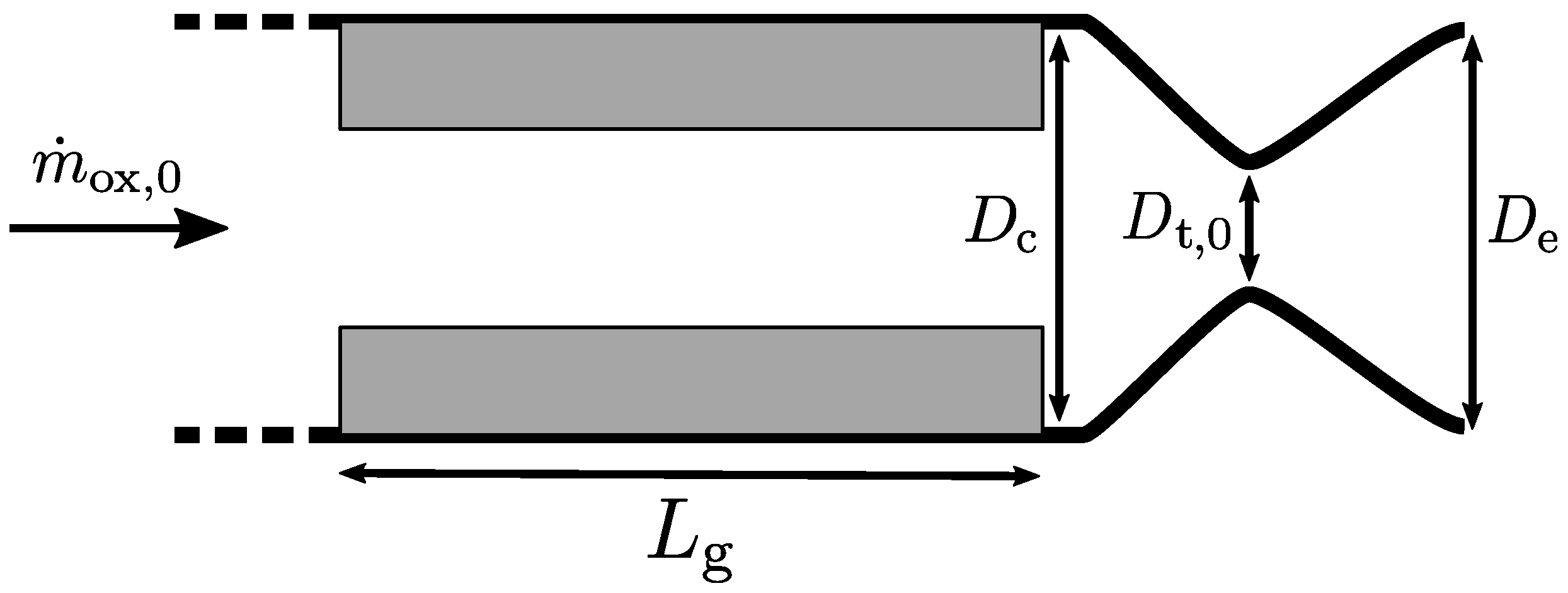
This set of parameters was chosen because it uniquely defines a preliminary HRE architecture, in line with the scope of a multidisciplinary optimization. Here, the nozzle geometry is determined by $D_{\mathrm{t},0}$ and $D_{\mathrm{e}}$, the combustion chamber and fuel grain by $L_{\mathrm{g}}$ and $D_{\mathrm{c}}$, and the engine operating conditions by the oxidizer mass flow rate ${\dot{m}}_{\mathrm{ox},0}$. A schematic description of the hybrid rocket unit design is shown in Figure 1.

In summary, the structural mass estimation relies on Mariotte’s equation for pressurized vessels (combustion chamber and tanks), empirical correlations from Larson et al. [49] and Saunders [50] for the nozzle and turbo-pump, respectively, and the model by Glatt [53] for insulation and shrouds. The turbo-pump feeding system, powered by hydrogen peroxide decomposition, is sized through a power balance as described above. While these models are approximate, they are considered adequate for the scope of a preliminary multidisciplinary optimization.

3. Machine Learning for HRE Performance Prediction

This section discusses the machine learning framework for creating a precise surrogate model to predict HRE performance.

Supervised Learning

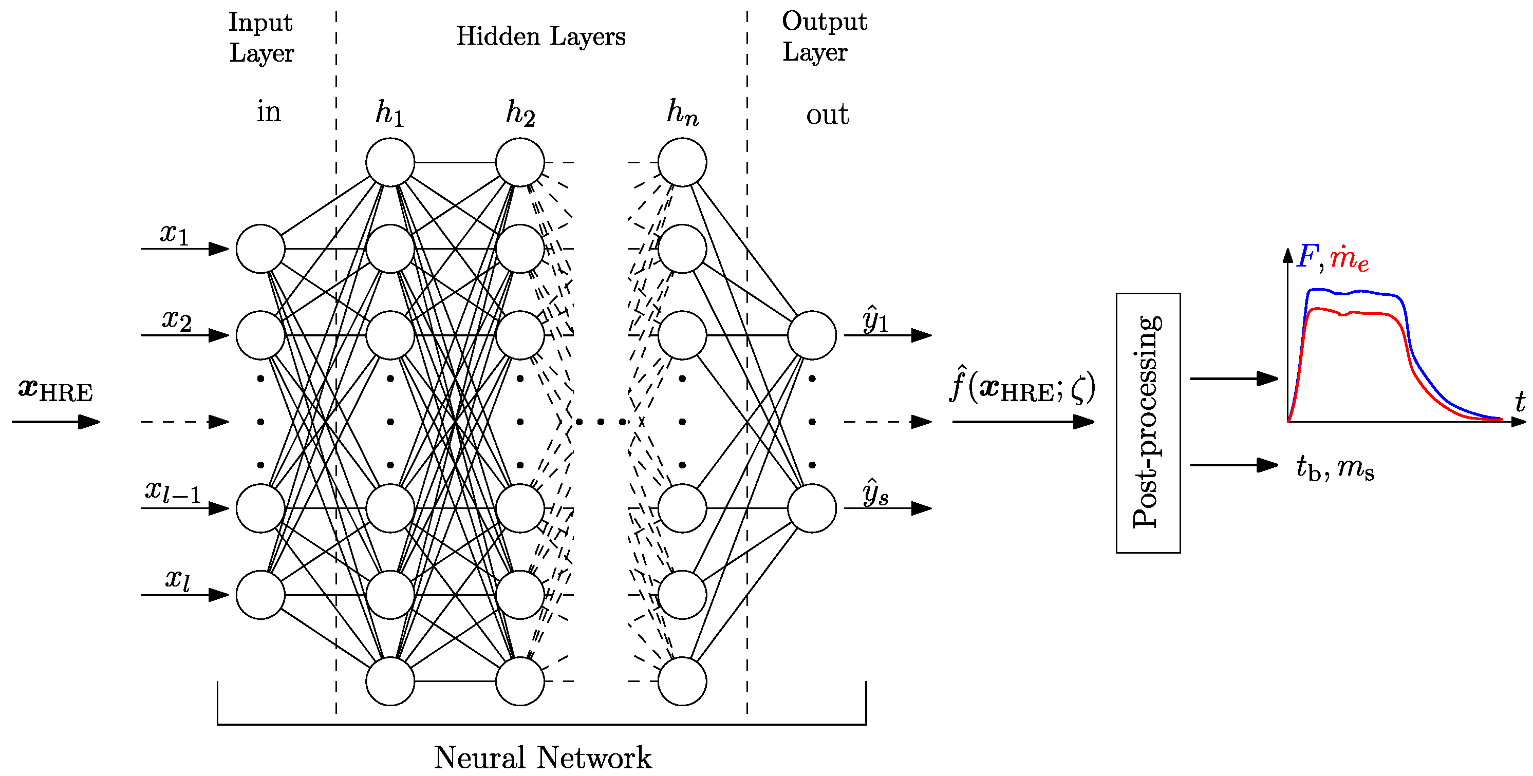
Feedforward neural networks (FNNs), inspired by brain structures, are MIMO computing systems composed of layers of neurons. Each neuron receives inputs from the previous layer and applies a non-linear activation function. The input and output layers are connected by hidden layers, as shown in Figure 2. FNNs have been proven to be universal function approximators, given sufficient data, neurons, and hidden units [57].

A supervised learning approach is generally used to teach the network how to correctly approximate a given function f based on input-output sample pairs. Given a data set, or training set, composed of N training examples $\mathcal{D}=\{({\mathit{x}}_1,{\mathit{y}}_1),({\mathit{x}}_2,{\mathit{y}}_2),\dots ,({\mathit{x}}_N,{\mathit{y}}_N)\}$, where ${\mathit{x}}_k$ is the feature vector of the k-th sample and ${\mathit{y}}_k=f\left({\mathit{x}}_k\right)$ the corresponding label, the objective is to learn a set of parameters $\zeta =\{({\mathit{W}}_{\mathrm{in}};{\mathit{b}}_{\mathrm{in}}),({\mathit{W}}_1;{\mathit{b}}_1),\dots ,({\mathit{W}}_n;{\mathit{b}}_n),({\mathit{W}}_{\mathrm{out}};{\mathit{b}}_{\mathrm{out}})\}$ such that the function

$$\widehat{f}(\mathit{x};\zeta )=f^o({\mathit{W}}_{\mathrm{out}}^T{f}^n({\mathit{W}}_n^T...f^1({\mathit{W}}_1^T{f}^i({\mathit{W}}_{\mathrm{in}}^T\mathit{x}+{\mathit{b}}_{\mathrm{in}})+{\mathit{b}}_1)+...+{\mathit{b}}_n)+{\mathit{b}}_{\mathrm{out}})$$

(20)

approximates as good as possible the “original” function f. The j-th column of the matrix ${\mathit{W}}_k$ represents the set of weights of the j-th neuron in the k-th layer, while the j-th element of the vector ${\mathit{b}}_k$ the corresponding bias. $f^k$, instead, is the activation function used in the k-th layer neurons. The dimensions of each ${\mathit{W}}_k$ matrix vary depending on the layer. The number of rows corresponds to the number of inputs (i.e., the number of neurons in the preceding layer), while the number of columns corresponds to the number of neurons in the current layer. Note that the number of neurons in the input and output layers, associated with ${\mathit{W}}_{\mathrm{in}}$ and ${\mathit{W}}_{\mathrm{out}}$, respectively, is equal to the number of inputs and outputs of the neural network. Consequently, the dimensions of these matrices are $1\times N_{\mathrm{in}}$ for ${\mathit{W}}_{\mathrm{in}}$ and $N_h^{\left(L\right)}\times N_{\mathrm{out}}$ for ${\mathit{W}}_{\mathrm{out}}$, where $N_{\mathrm{in}}$ and $N_{\mathrm{out}}$ denote the number of network inputs and outputs, respectively, and $N_h^{\left(L\right)}$ denotes the number of neurons in the last hidden layer. The number of rows for ${\mathit{W}}_{\mathrm{in}}$ is 1 since each neuron of this layer takes a single neural network input. The procedure involves splitting the initial data set into a training set $\mathcal{T}$ and a validation set $\mathcal{V}$, with sizes $N_{\mathcal{T}}={\eta }_{t}N$ and $N_{\mathcal{V}}=N-N_{\mathcal{T}}$, respectively, where ${\eta }_t$ is a hyper-parameter called “train fraction”. The training set is used to train the network, while the validation set is used to assess the network performance on unseen data. Training examples in the training set are organized into batches, each containing $n_b$ elements ($n_b$ is a hyper-parameter), and the network parameters $\zeta$ are first randomly initialized. The optimization of the parameters $\zeta$ is done by minimizing the mean squared error (MSE) between the network outputs and the training examples using stochastic gradient descent (SGD):

$$\begin{array}{cc}\hfill {\mathrm{MSE}}^{\left(1\right)}\left(\zeta \right)& ={\displaystyle \frac{1}{n_b}}\sum _{i=k_1}^{k_{n_b}}{\Vert {\mathit{y}}_i-\widehat{f}({\mathit{x}}_i;\zeta )\Vert }^2\hfill \end{array}$$

(21)

$$\begin{array}{cc}\hfill \zeta & =\zeta -\alpha {\nabla }_{\zeta }{\mathrm{MSE}}^{\left(1\right)}\left(\zeta \right)\hfill \end{array}$$

(22)

$$\begin{array}{cc}\hfill {\mathrm{MSE}}^{\left(2\right)}\left(\zeta \right)& ={\displaystyle \frac{1}{n_b}}\sum _{i=k_{n_b+1}}^{k_{2n_b}}{\Vert {\mathit{y}}_i-\widehat{f}({\mathit{x}}_i;\zeta )\Vert }^2\hfill \end{array}$$

(23)

$$\zeta =\zeta -\alpha {\nabla }_{\zeta }{\mathrm{MSE}}^{\left(2\right)}\left(\zeta \right)$$

(24)

$$\dots$$

$$\begin{array}{cc}\hfill {\mathrm{MSE}}^{\left(B\right)}\left(\zeta \right)& ={\displaystyle \frac{1}{n_b}}\sum _{i=k_{\left(B-1\right)n_b+1}}^{k_{N_T}}{\Vert {\mathit{y}}_i-\widehat{f}({\mathit{x}}_i;\zeta )\Vert }^2\hfill \end{array}$$

(25)

$$\begin{array}{cc}\hfill \zeta & =\zeta -\alpha {\nabla }_{\zeta }{\mathrm{MSE}}^{\left(B\right)}\left(\zeta \right)\hfill \end{array}$$

(26)

This B-step gradient descent optimization is repeated for M total training epochs (hyper-parameter). In this work, the Adam (adaptive moment estimation) [58] SGD algorithm is used for optimization, with a linear learning rate $\alpha ={\alpha }_i+({\alpha }_f-{\alpha }_i)m/M$, with m the current training epoch, and with ${\alpha }_i$ and ${\alpha }_f$ being hyper-parameters. The network hyper-parameters have been selected according to previous studies performed in Zavoli et al. [28,29] and are shown in

Table 2. Hyper-parameters of the supervised learning algorithm.

Hyper-Parameter	Symbol	Value
Initial learning rate	${\alpha }_i$	1 × 10−4
Final learning rate	${\alpha }_f$	1 × 10−7
Train fraction	${\eta }_t$	0.99
Batch size	$n_b$	512
N. of training epochs	M	1000

.

Figure 2 illustrates the architecture of the neural network used as a surrogate model for HRE performance prediction. The network takes the motor design variables ${\mathit{x}}_{\mathrm{HRE}}$ as input and returns 10 scalar outputs: the engine burning time $t_{\mathrm{b}}$, the dry mass $m_{\mathrm{s}}$, and the coefficients of two cubic polynomials that approximate the thrust $F\left(t\right)$ and total mass flow rate $\dot{m}\left(t\right)$ curves of the engine. With this approach, each time-dependent curve is parameterized by the network as:

$$\begin{array}{c}F\left(t\right)=a_F{x}^3+b_F{x}^2+c_{F}x+d_F\\ \dot{m}\left(t\right)=a_{\dot{m}}{x}^3+b_{\dot{m}}{x}^2+c_{\dot{m}}x+d_{\dot{m}}\\ \mathrm{with}x=t/t_{\mathrm{b}},x\in (0,1)\hfill \end{array}$$

(27)

4. Launch Vehicle Configuration

Before describing the ascent trajectory mathematical model, the general LV configuration must be defined. Assuming equal performance and structural coefficients for each stage, a simple analysis of the behavior of the payload ratio $\lambda$ with respect to the number of stages can be performed using Tsiolkovsky’s equation:

$$\lambda ={\left[\left(1+k_{\mathrm{t}}\right)e^{-\mathrm{\Delta }{v}_{\mathrm{pr}}/\left(I_{\mathrm{sp}}{g}_{0}N\right)}-k_{\mathrm{t}}-k_{\mathrm{e}}\right]}^N$$

(28)

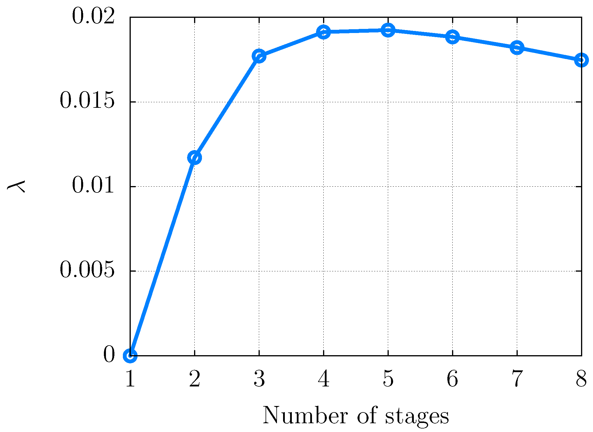
where $\mathrm{\Delta }{v}_{\mathrm{pr}}$ is the propulsive velocity increase for the target mission, N is the number of stages of the LV, $I_{\mathrm{sp}}$ is the specific impulse of the stage, $k_{\mathrm{t}}=m_{\mathrm{s},\mathrm{tk}}/m_{\mathrm{p}}$ is the relationship between the propellant-related masses over the propellant mass of the stage, and $k_{\mathrm{e}}=\left(m_{\mathrm{s}}-m_{\mathrm{s},\mathrm{tk}}\right)/m_{0,i}$ is the relationship between the engine weight of a stage over the mass of the corresponding sub-rocket. After a brief tuning for the problem at hand, values of $\mathrm{\Delta }{v}_{\mathrm{pr}}=9.7$ km/s, $I_{\mathrm{sp}}=320$ s, $k_{\mathrm{t}}=0.061$, and $k_{\mathrm{e}}=0.057$ have been selected. Results of the analysis are shown in Figure 3. The highest payload ratio is achieved with five stages. However, the payload gain from increasing the number of stages beyond three is minimal (+0.6% from two to three stages, +0.142% from three to four, and +0.011% from four to five), making the performance boost insufficient to justify the increased complexity. Moreover, as this preliminary analysis does not take into account the mass of the inter-stages, the payload ratio is expected to further decrease with the number of stages. A three-stage configuration is thus selected for the analyzed mission.

To finalize the general LV configuration, the number of HRE units for each stage must be chosen. A good starting point is to compute the optimal $\mathrm{\Delta }v$ partitioning for the selected three-stage configuration by minimizing the following cost function (the negative logarithm of the launch vehicle payload ratio):

$$\mathrm{\Lambda }\left(\mathrm{\Delta }{v}_i\right)=-\ln \left(\prod _{i=1}^3{\displaystyle \frac{e^{-\mathrm{\Delta }{v}_i/\left(I_{\mathrm{sp},i}{g}_0\right)}-k_{\mathrm{s},i}}{1-k_{\mathrm{s},i}}}\right)$$

(29)

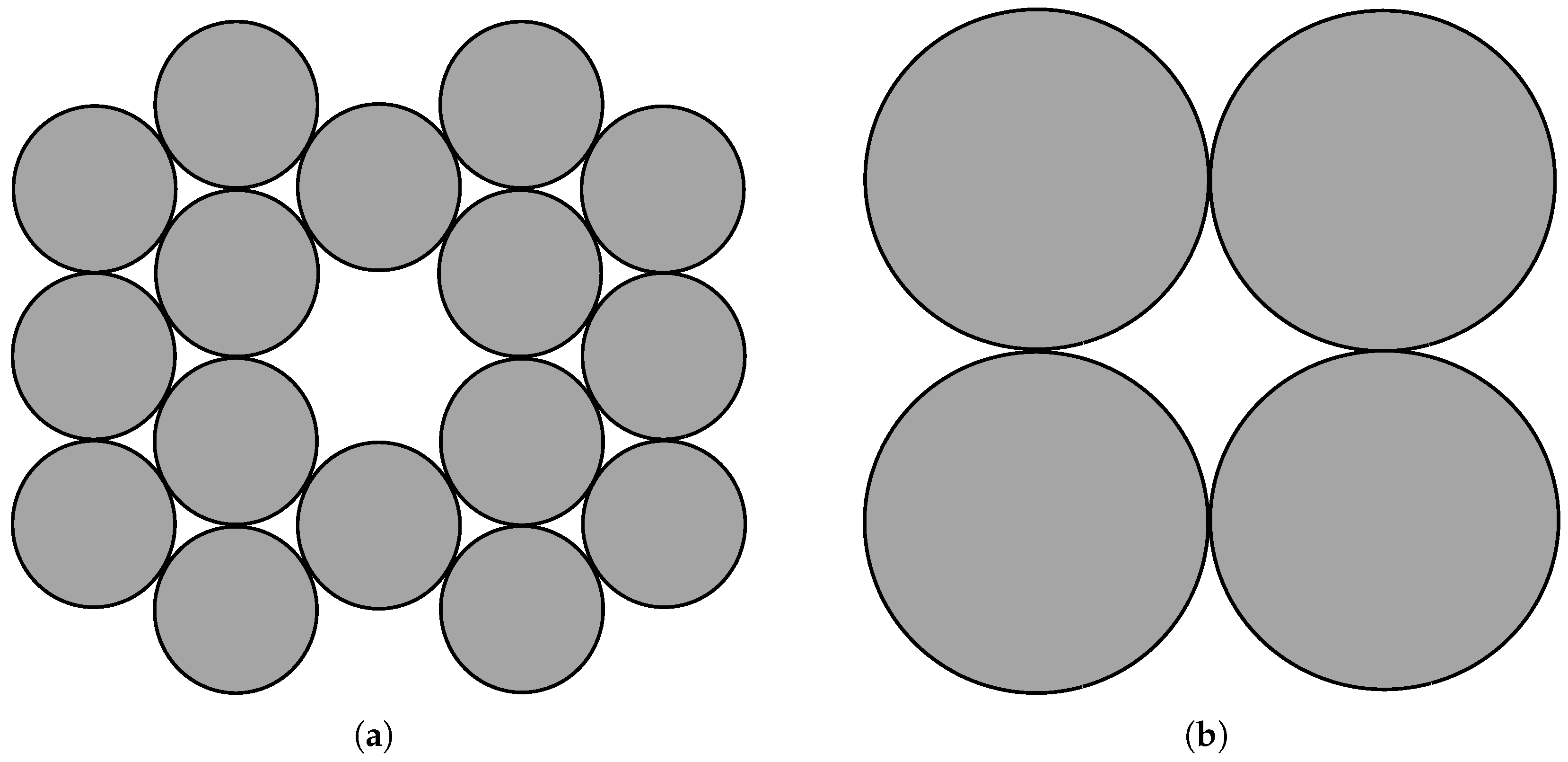
where $\mathrm{\Delta }{v}_i$, $I_{\mathrm{sp},i}$, and $k_{\mathrm{s},i}$ are, respectively, the velocity increase (optimized), specific impulse, and structural coefficient of the i-th stage, with ${\displaystyle k_{\mathrm{s},i}={\displaystyle \frac{m_{\mathrm{s},i}}{m_{\mathrm{s},i}+m_{\mathrm{p},i}}}}$. Realistic values for $I_{\mathrm{sp},i}$ and $k_{\mathrm{s},i}$ have been assumed after a brief preliminary analysis. To reproduce the optimal $\mathrm{\Delta }v$ partitioning obtained by minimizing Equation (29) ($\mathrm{\Delta }{v}_1/\mathrm{\Delta }{v}_{\mathrm{pr}}=0.28$, $\mathrm{\Delta }{v}_2/\mathrm{\Delta }{v}_{\mathrm{pr}}=0.37$, $\mathrm{\Delta }{v}_3/\mathrm{\Delta }{v}_{\mathrm{pr}}=0.35$, with $\mathrm{\Delta }{v}_{\mathrm{pr}}=9.7$ km/s) and assuming the upper stage to be constituted by a single HRE unit, approximately 12 units are needed for the first stage, and 4 units for the second stage. However, as the analysis does not take into account the effects of thrust, a 16-4-1 configuration is ultimately chosen. This adjustment is made to maximize thrust during the first stage flight, thereby reducing gravitational losses. A higher quantity of units cannot be employed for the first stage to ensure compliance with the axial acceleration constraint, which will be introduced in the following section. Disposition of HRE units in the first and second stage is shown in Figure 4.

The diameters of the stages can be computed as:

$$D_{\mathrm{stage},i}={\xi }_i\max \left(D_{\mathrm{c}},D_{\mathrm{e},i}\right)$$

(30)

where the packing ratio ${\xi }_i$ is equal to 4.62 for the first stage and 2.42 for the second stage. Note that, although maintaining the alignment of such a large number of engines might pose technical challenges, this paper focuses on theoretical analysis and does not address such a practical issue.

5. Flight Trajectory Model

This section provides a description of the ascent trajectory model, presenting the equations of motion, the adopted flight strategy, and the mission constraints, followed by the formulation of the integrated optimization problem.

5.1. Dynamical Model

A three-dimensional (3-DoF) point-mass model is employed. Under this hypothesis, the LV is considered always aligned with the direction of thrust, assuming infinitely fast attitude dynamics. The rocket state at any time is defined by position vector $\mathit{r}$, velocity vector $\mathit{v}$, and mass m. The equations of motion in an inertial reference frame are written as:

$$\begin{array}{cc}\hfill \dot{\mathit{r}}& =\mathit{v}\hfill \end{array}$$

(31)

$$\begin{array}{cc}\hfill \dot{\mathit{v}}& =\mathit{g}+{\displaystyle \frac{\mathit{D}+\mathit{F}}{m}}\hfill \end{array}$$

(32)

$$\begin{array}{cc}\hfill \dot{m}& =-{\dot{m}}_{\mathrm{e}}\hfill \end{array}$$

(33)

The Earth is approximated as a sphere, with the gravitational acceleration vector represented as ${\displaystyle \mathit{g}=-\frac{\mu }{r^3}\mathit{r}}$, where $\mu$ is the Earth’s gravitational constant. Air density ${\rho }_{\mathrm{a}}$, pressure $p_{\mathrm{a}}$, and temperature $T_{\mathrm{a}}$ are evaluated based on the altitude h, following the U.S. Standard Atmosphere 1976 model [59]. It is assumed that the atmosphere rotates rigidly with the Earth at ${\mathit{\omega }}_E=7.2921\times {10}^{-5}\mathrm{rad}/\mathrm{s}$. Thus, the relative velocity of the vehicle with respect to the atmosphere is computed as ${\mathit{v}}_{\mathrm{rel}}=\mathit{v}-{\mathit{\omega }}_E\times \mathit{r}$. Atmospheric drag is evaluated as:

$$\mathit{D}=-{\displaystyle \frac{1}{2}}{\rho }_{\mathrm{a}}{S}_{\mathrm{ref}}{C}_D\left(M\right)v_{\mathrm{rel}}{\mathit{v}}_{\mathrm{rel}}$$

(34)

where $S_{\mathrm{ref}}$ denotes the vehicle cross-sectional area and $C_D$ is the drag coefficient. Lift force is neglected because it is deemed of minor importance for the current analysis. The drag coefficient is assumed solely dependent on the Mach number of the LV and is tabulated based on data from known launcher flights for similar applications. The thrust force $\mathit{F}$ generated by the LV motors is expressed as:

$$\mathit{F}=\left(F_{\mathrm{vac}}-p_{\mathrm{a}}{A}_{\mathrm{e}}\right)\widehat{\mathit{F}}$$

(35)

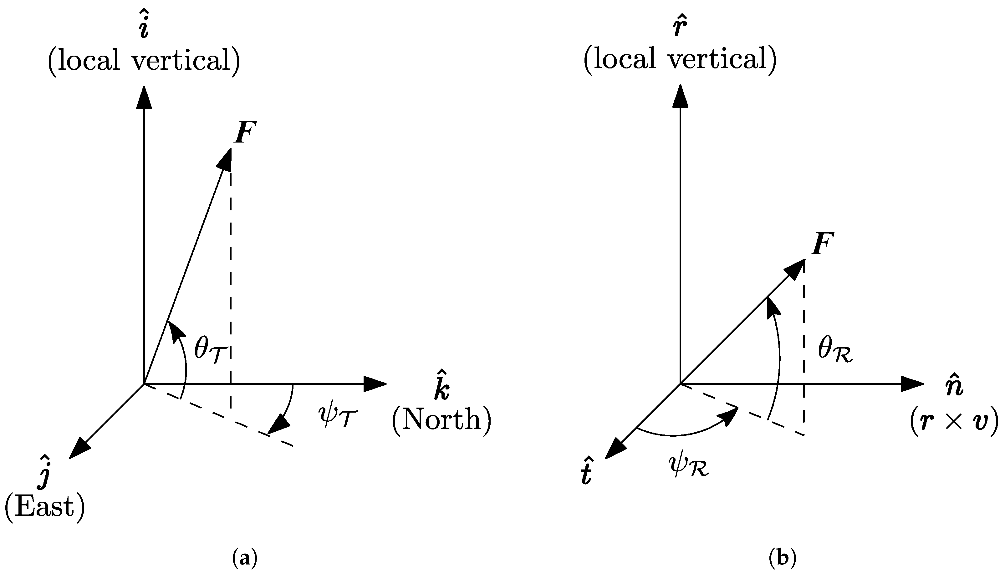
where $A_{\mathrm{e}}$ is the nozzle exit area and $F_{\mathrm{vac}}$ denotes the thrust in vacuum. When the launcher is still in close proximity to the launch base, the direction of thrust is defined in a topocentric reference frame, fixed relative to the launch base, ${\mathcal{F}}_{\mathcal{T}}=(\widehat{\mathit{i}},\widehat{\mathit{j}},\widehat{\mathit{k}})$ (Figure 5a).

$$\widehat{\mathit{F}}=sin{\theta }_{\mathcal{T}}\widehat{\mathit{i}}+cos{\theta }_{\mathcal{T}}sin{\psi }_{\mathcal{T}}\widehat{\mathit{j}}+cos{\theta }_{\mathcal{T}}cos{\psi }_{\mathcal{T}}\widehat{\mathit{k}}$$

(36)

where ${\theta }_{\mathcal{T}}$ and ${\psi }_{\mathcal{T}}$ indicate the elevation and azimuth angles in this frame. During the flight in the exo-atmospheric region, thrust is defined with in-plane and out-of-plane angles ${\theta }_{\mathcal{R}}$ and ${\psi }_{\mathcal{R}}$ of a radial-transverse-normal (RTN) local reference frame ${\mathcal{F}}_{\mathcal{R}}=(\widehat{\mathit{r}},\widehat{\mathit{t}},\widehat{\mathit{n}})$ (Figure 5b).

$$\widehat{\mathit{F}}=sin{\theta }_{\mathcal{R}}\widehat{\mathit{r}}+cos{\theta }_{\mathcal{R}}cos{\psi }_{\mathcal{R}}\widehat{\mathit{t}}+cos{\theta }_{\mathcal{R}}sin{\psi }_{\mathcal{R}}\widehat{\mathit{n}}$$

(37)

5.2. Flight Strategy

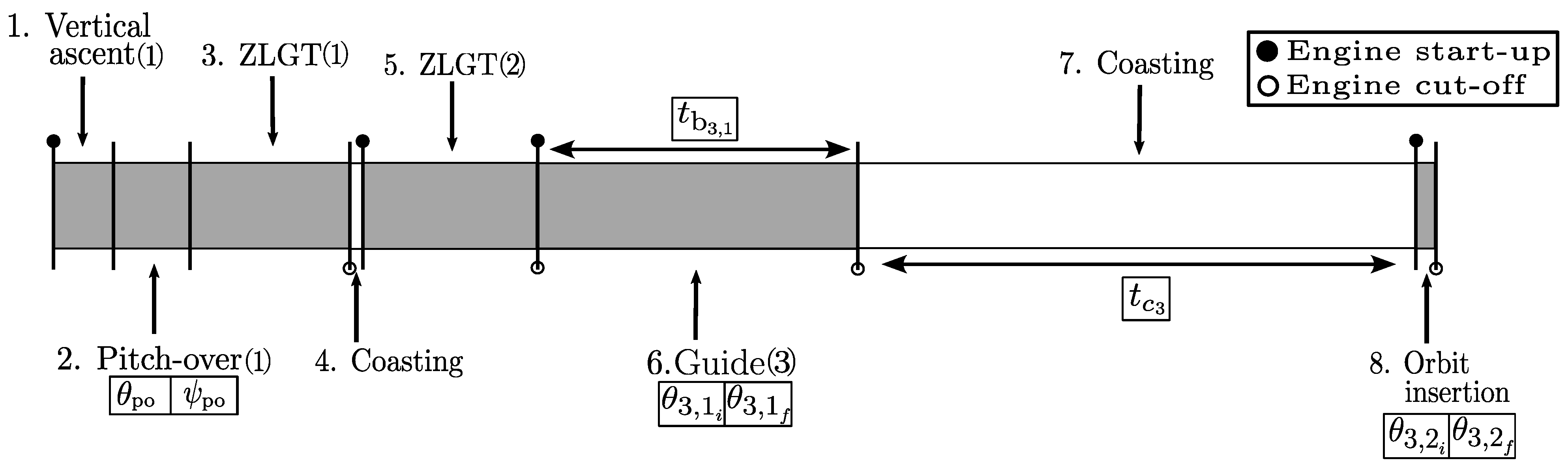
A realistic flight strategy is considered. The ascent trajectory is divided into several phases, each characterized by a specific control law, with a schematic representation shown in Figure 6. The first phase is a vertical ascent, where the thrust is directed radially until a certain distance from the launch base is reached. Next, a pitch-over maneuver is performed to rotate the LV and align it with the desired orbital plane. In a simplified 3-degree-of-freedom model, this maneuver is represented by a linearly decreasing thrust elevation angle and a constant thrust azimuth angle. The LV then follows a zero-lift gravity-turn (ZLGT) trajectory. During this phase, the thrust vector is aligned with the relative velocity to prevent the generation of lift or side force. The gravity gradually rotates the velocity vector downward. After a brief coasting, with a duration of one second to allow stage separation, the second stage is ignited, and the LV continues to follow a ZLGT trajectory. The fairing is jettisoned at the second stage cut-off. Finally, the third stage performs a burn to transition the LV into a Hohmann-like trajectory. The pitch program during this phase follows a linear law, with a null azimuth angle. After a long coasting phase, a second burn of the third stage, with another linear variation of the thrust elevation angle and a null azimuth angle, is executed to circularize the orbit and place the payload into the desired target orbit.

5.3. Constraints and Objective Function

The initial conditions of the launch vehicle depend on the geographical position of the launch base. The initial position ${\mathit{r}}_0$ is the base position, and the inertial velocity ${\mathit{v}}_0$ can be determined as ${\mathit{\omega }}_E\times {\mathit{r}}_0$. The problem goal is to maximize the LV payload $m_{\mathrm{u}}$. Hence, the objective function to minimize is designed as $-m_{\mathrm{u}}$. The LV wet mass is constrained to be equal to $m_{0,\mathrm{wet}}=m_0-m_{\mathrm{u}}$ = 55,000 kg, where $m_0$ is the lift-off mass, chosen for comparison with the declared characteristics of Vega C Light [60]. Terminal constraints are imposed to ensure payload injection into a circular orbit with a desired radius, $\tilde{r}$, and inclination, $\tilde{i}$. Tolerances, $\delta r$ and $\delta i$, are set for periapsis radii, apoapsis radii, and inclination. The right ascension of the ascending node is not directly enforced, as it can be easily adjusted by selecting the launch time. Dimensional constraints are also enforced to guarantee the LV compactness. Specifically, the diameter of a stage cannot be larger than the diameter of the preceding stage $D_{\mathrm{stage},\mathrm{i}}\le D_{\mathrm{stage},\mathrm{i}-1}$, and the nozzle exit diameter of first-stage HRE units must be smaller than the units case diameter $D_{\mathrm{c}}\ge D_{\mathrm{e},1}$. To ensure the structural integrity of the vehicle and payload during ascent, constraints on maximum axial acceleration, $a_x=\dot{\mathit{v}}·\widehat{\mathit{F}}/g_0$, and maximum heat flux exposure, ${\varphi }_q=0.5{\rho }_a{v}_{\mathrm{rel}}^3$, after fairing jettisoning are enforced in the optimization, set, respectively, to 5 g and 900 W/m². Maximum dynamic pressure and max-Q$\alpha$ are instead checked a posteriori, as they are considered of minor importance for the problem at hand.

5.4. Optimization

The resulting multidisciplinary optimization problem involves finding optimal values for the single HRE unit design parameters ${\mathit{x}}_{\mathrm{HRE}}$ (up to the nozzle throat), along with the optimal exit nozzle diameters for each of the three stages $D_{\mathrm{e},1}$, $D_{\mathrm{e},2}$, and $D_{\mathrm{e},3}$. This results in a vector of 7 design parameters:

$${\mathit{x}}_{\mathrm{HRE}}=[L_{\mathrm{g}},D_{\mathrm{c}},D_{\mathrm{t},0},{\dot{m}}_{\mathrm{ox},0},D_{\mathrm{e},1},D_{\mathrm{e},2},D_{\mathrm{e},3}]$$

(38)

where the design vector in Equation (19) is extended to include the three different exit diameters of the HRE unit used in each stage. Note that the adoption of clustering significantly streamlines the optimization process, as only the reference HRE unit has to be optimized instead of a set of HRE design parameters for each stage of the launch vehicle. For the same reason, only one surrogate model needs to be trained. The reference HRE unit of the cluster is optimized within a design space selected to provide average thrusts between 40 and 70 kN, with operating pressures between 20 and 100 bar. The resulting domain for ${\mathit{x}}_{\mathrm{HRE}}$ is shown in

Table 3. Range of variation of the HRE design parameters.

Quantity	Min	Max	Unit
$L_{\mathrm{g}}$	2.2	4.0	m
$D_{\mathrm{c}}$	0.3	0.7	m
$D_{\mathrm{t},0}$	0.06	0.15	m
${\dot{m}}_{\mathrm{ox},0}$	5	20	kg/s
$D_{\mathrm{e},i}$	0.212	1.897	m

.

Optimal values for flight mechanics variables, ${\mathit{x}}_{\mathrm{flight}}$, and thrust direction variables, ${\mathit{x}}_{\mathrm{guide}}$, also need to be determined. The flight design variables comprise the duration of the third stage first burn $t_{{\mathrm{b}}_{3,1}}$ and the duration of the following coasting phase $t_{c_3}$. The duration of the orbit insertion phase (second burn of the third stage) can be easily computed as $t_{{\mathrm{b}}_{3,2}}=t_{{\mathrm{b}}_3}-t_{{\mathrm{b}}_{3,1}}$:

$${\mathit{x}}_{\mathrm{flight}}=[t_{{\mathrm{b}}_{3,1}},t_{c_3}]$$

(39)

Lastly, 6 design variables are required to parameterize the thrust direction of the launch vehicle. These include the elevation and azimuth at the end of the pitch-over phase, ${\theta }_{\mathrm{po}}$ and ${\psi }_{\mathrm{po}}$, the elevation at the beginning and the elevation at the end of the upper stage guidance, ${\theta }_{{3,1}_i}$ and ${\theta }_{{3,1}_f}$, and the elevation angle at both the beginning and the end of the final orbital injection, that is, ${\theta }_{{3,2}_i}$ and ${\theta }_{{3,2}_f}$. Thus:

$${\mathit{x}}_{\mathrm{guide}}=[{\theta }_{\mathrm{po}},{\psi }_{\mathrm{po}},{\theta }_{{3,1}_i},{\theta }_{{3,1}_f},{\theta }_{{3,2}_i},{\theta }_{{3,2}_f}]$$

(40)

The resulting full optimization vector for the entire MDO problem includes 15 design parameters:

$${\mathit{x}}_{\mathrm{opt}}=[L_{\mathrm{g}},D_{\mathrm{c}},D_{\mathrm{t},0},{\dot{m}}_{\mathrm{ox},0},D_{\mathrm{e},1},D_{\mathrm{e},2},D_{\mathrm{e},3},t_{{\mathrm{b}}_{3,1}},t_{c_3},{\theta }_{\mathrm{po}},{\psi }_{\mathrm{po}},{\theta }_{{3,1}_i},{\theta }_{{3,1}_f},{\theta }_{{3,2}_i},{\theta }_{{3,2}_f}]$$

(41)

The optimization problem is solved using EOS (evolutionary optimization at Sapienza), an in-house evolutionary optimization code for constrained global optimization [61]. This code utilizes a multi-population, self-adaptive, $\epsilon$-constrained differential evolution algorithm with an island model for parallel execution. Previous successful applications of EOS to space trajectory optimization problems include [18,28,29,62,63].

6. Results

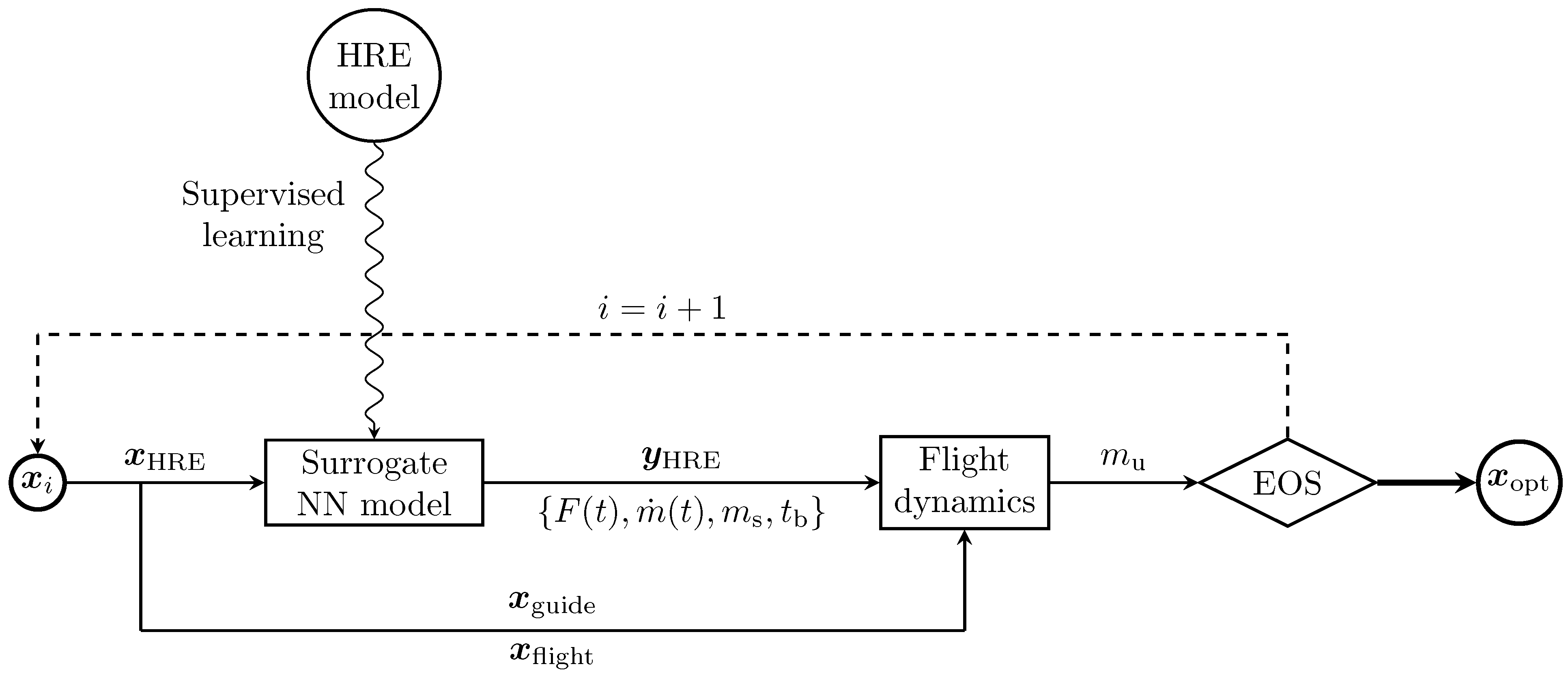
This section presents the results obtained for the formulated multidisciplinary optimization problem. A schematic representation of the procedure is shown in Figure 7.

A preliminary analysis has been carried out to assess the most suitable network architecture and number of input-output samples to ensure the reliability of the surrogate model.

6.1. Surrogate NN-Based HRE Model

Training of the NN-based surrogate HRE model has been performed with a random distribution across the design space of input-output samples, with the sample count ranging from 50,000 (50k) to 1,000,000 (1000k). An additional dataset ${\mathcal{T}}_{\mathrm{s}}$ comprising 10,000 samples has also been generated to evaluate the surrogate model performance. The network architectures considered for the present investigation are reported in

Table 4. Neurons in each layer for the investigated network configurations (I: Input, O: Output, h: hidden layer), and total number of trainable parameters, $N_{\mathrm{train}}$.

Configuration	I	h1	h2	h3	h4	h5	h6	h7	h8	h9	O	${\mathit{N}}_{\mathit{train}}$
Net1	5	64	256	64	-	-	-	-	-	-	11	34,217
Net2	5	64	256	256	64	-	-	-	-	-	11	100,009
Net3	5	64	256	512	256	64	-	-	-	-	11	297,129
Net4	5	64	256	512	512	256	64	-	-	-	11	559,785
Net5	5	64	256	512	1024	512	256	64	-	-	11	1,347,241
Net6	5	64	256	512	1024	1024	512	256	64	-	11	2,396,841
Net7	5	64	256	512	1024	2048	1024	512	256	64	11	5,544,617

. The activation function is the rectified linear unit for all neurons in the hidden layers, while the output neurons feature a linear activation function.

Regardless of the specific configuration, a symmetric pyramidal (or inverse hourglass) network structure has been adopted, as it enables a gradual increase in feature abstraction, followed by a symmetrical compression of the information back into a low-dimensionality vector. This design enables the network to learn progressively richer feature representations in the expansion phase and then compress them into distilled, high-level features before the output. Such architectures, commonly used in representation learning, were found effective in previous works on this topic [28,29,30].

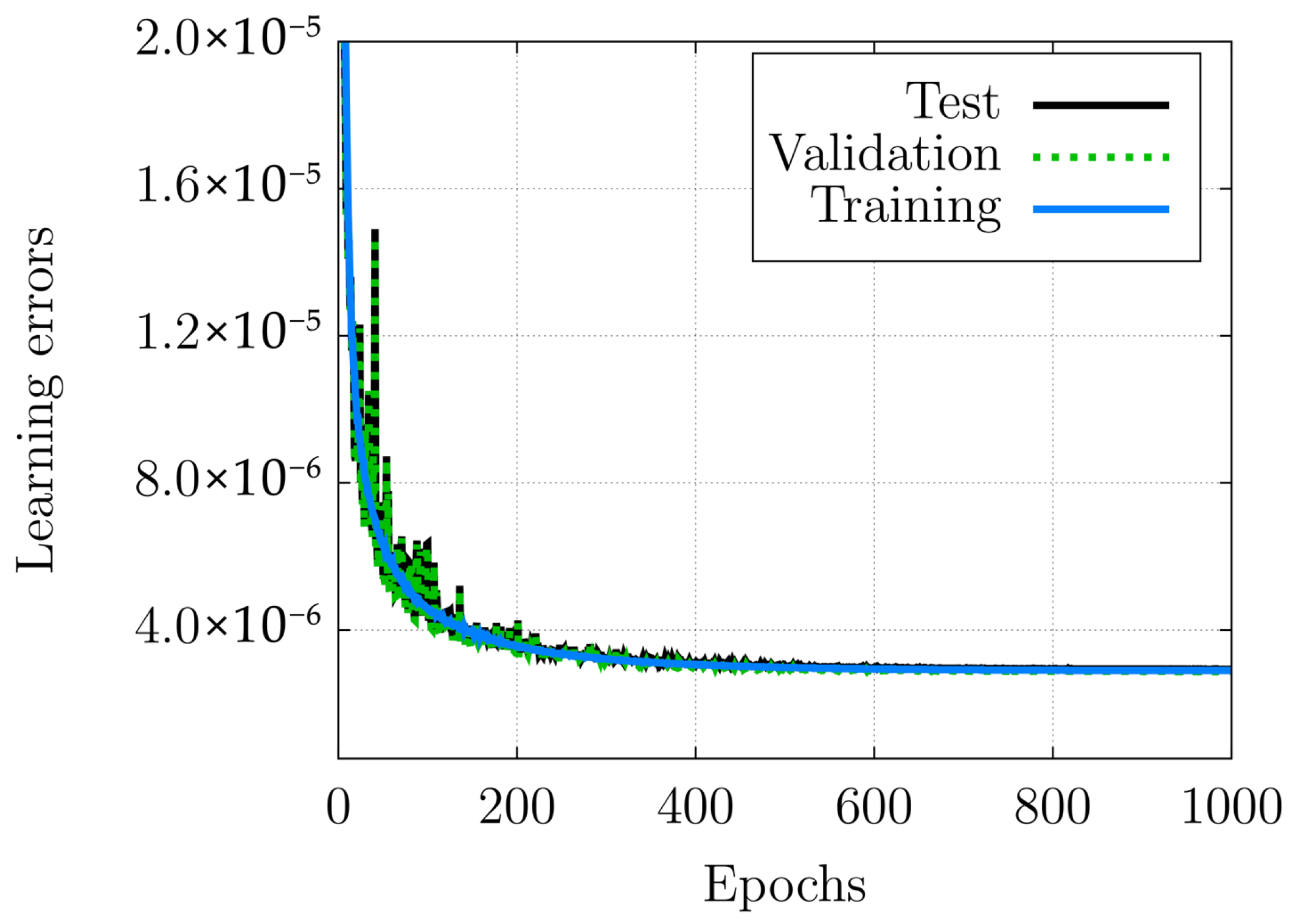
Training, validation, and test errors (or losses) for an intermediate-size network (Net4, as per Table 4, trained using 500k samples) are shown in Figure 8. Errors are computed as the mean squared error (MSE) between the true and predicted outputs, normalized between 0 and 1, with respect to the training set $\mathcal{T}$, validation set $\mathcal{V}$, and test set ${\mathcal{T}}_{\mathrm{s}}$, respectively (as per Equations (21)–(25)). Errors show a clear plateau-like behavior, with a monotonically decreasing trend followed by an asymptotic value, reached approximately around 600 epochs.

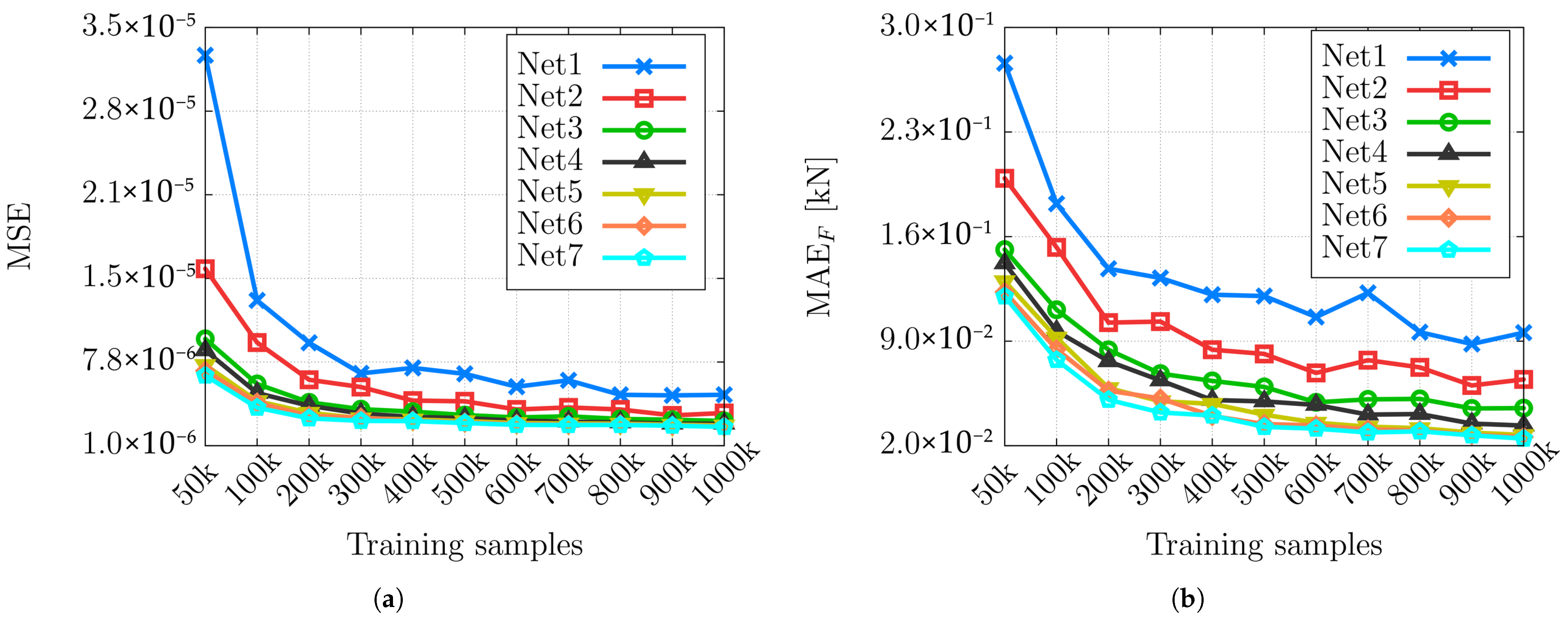
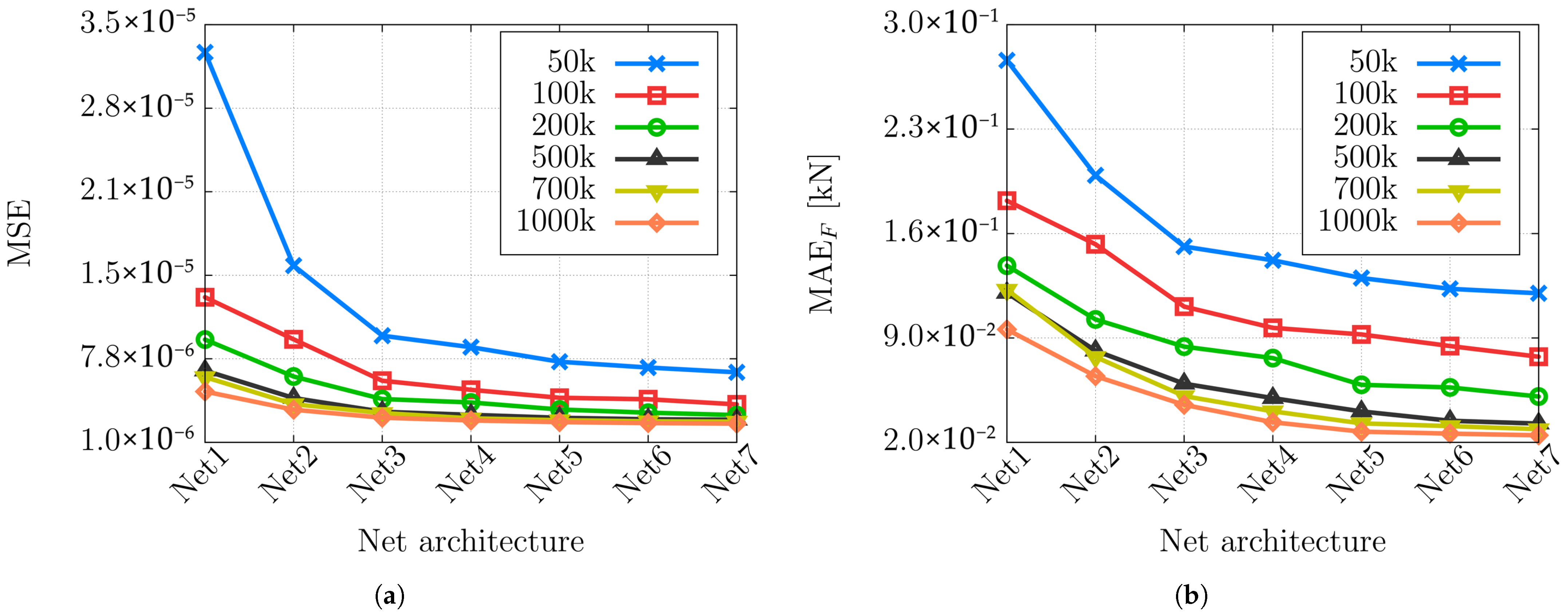
Specific metrics to assess the surrogate model performance with respect to HRE physics are also introduced: (i) ${\mathrm{MAE}}_F$, the mean absolute error between the true thrust curve (computed with the internal ballistics model, Section 2) and the thrust curve predicted by the NN using cubic polynomials, evaluated at 40 different points in time. (ii) ${\mathrm{MAE}}_{\dot{m}}$, the mean absolute error between the true and predicted mass flow rate curves, computed in the same manner as ${\mathrm{MAE}}_F$. (iii) ${\mathrm{MAE}}_{t_{\mathrm{b}}}$, the mean absolute error between the predicted and true engine burning time. (iv) ${\mathrm{MAE}}_{m_{\mathrm{s}}}$, between predicted and true structural (dry) mass of the motor. Note that a test dataset ${\mathcal{T}}_{\mathrm{s}}$ with 10,000 samples is assumed statistically sufficient to consider the mean absolute error as a reliable and robust metric for the surrogate model accuracy. Test loss and ${\mathrm{MAE}}_F$ of the trained networks for different numbers of training samples and for different network architectures are shown in Figure 9 and Figure 10.

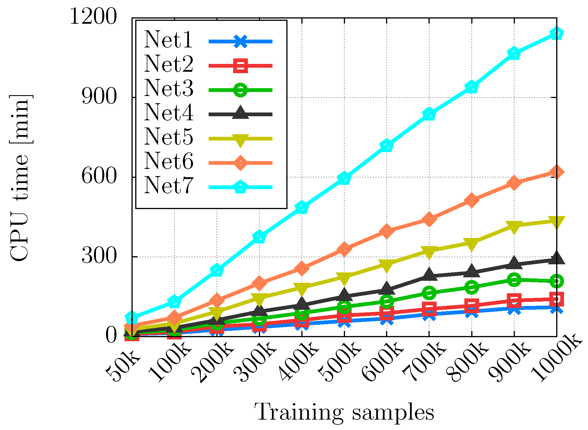
Results show a clear relationship between the dimensions of the training set, the architecture complexity, and the accuracy of the NN. In general, the accuracy tends to grow with the number of training samples. However, the benefits of using a larger dataset decrease with the dimensions of the dataset itself. A similar behavior can be seen with respect to the architecture complexity, with the prediction accuracy improving with the number of hidden layers, but with the benefits of adding layers decreasing with their number. Trends shown in Figure 9 and Figure 10 for test loss and ${\mathrm{MAE}}_F$ can be reproduced for each of the surrogate model performance metrics. It can be concluded that the relative improvement in prediction accuracy is quite small beyond intermediate-size networks and intermediate-size training datasets. For this reason, the 8-layer network architecture (Net4) and the training dataset with 500k samples are chosen as references for the present study. This choice is also considered cost-efficient, since the CPU time required to train the network grows roughly linearly with the dataset dimensions and exponentially with the network complexity, as shown in Figure 11.

Performance metrics for the configuration Net4 with different numbers of training samples are shown in

Table 5. Learning and performance parameters of the trained network for different numbers of training samples (Net4).

Training Dataset	Learning Errors			Propulsive Performance Metrics				CPU Time [min]
	Training	Validation	Test	${\mathbf{MAE}}_{\mathit{F}}$ [kN]	${\mathbf{MAE}}_{\dot{\mathit{m}}}$ [kg/s]	${\mathbf{MAE}}_{{\mathit{t}}_{\mathit{b}}}$ [s]	${\mathbf{MAE}}_{{\mathit{m}}_{\mathit{s}}}$ [kg]
50k	7.93 $\times {10}^{-6}$	9.07 $\times {10}^{-6}$	8.75 $\times {10}^{-6}$	1.42 $\times {10}^{-1}$	3.80 $\times {10}^{-2}$	4.16 $\times {10}^{-1}$	1.13 $\times {10}^0$	18.6
100k	5.04 $\times {10}^{-6}$	5.26 $\times {10}^{-6}$	5.28 $\times {10}^{-6}$	9.67 $\times {10}^{-2}$	2.40 $\times {10}^{-2}$	2.97 $\times {10}^{-1}$	9.03 $\times {10}^{-1}$	32.7
200k	4.08 $\times {10}^{-6}$	4.31 $\times {10}^{-6}$	4.25 $\times {10}^{-6}$	7.65 $\times {10}^{-2}$	1.89 $\times {10}^{-2}$	2.47 $\times {10}^{-1}$	6.94 $\times {10}^{-1}$	61.9
300k	3.50 $\times {10}^{-6}$	3.63 $\times {10}^{-6}$	3.61 $\times {10}^{-6}$	6.37 $\times {10}^{-2}$	1.54 $\times {10}^{-2}$	2.22 $\times {10}^{-1}$	6.14 $\times {10}^{-1}$	94.4
400k	3.24 $\times {10}^{-6}$	3.33 $\times {10}^{-6}$	3.34 $\times {10}^{-6}$	5.06 $\times {10}^{-2}$	1.24 $\times {10}^{-2}$	2.01 $\times {10}^{-1}$	5.47 $\times {10}^{-1}$	118.2
500k	3.18 $\times {10}^{-6}$	3.23 $\times {10}^{-6}$	3.24 $\times {10}^{-6}$	4.97 $\times {10}^{-2}$	1.20 $\times {10}^{-2}$	1.81 $\times {10}^{-1}$	4.99 $\times {10}^{-1}$	150.8
600k	2.98 $\times {10}^{-6}$	3.01 $\times {10}^{-6}$	3.04 $\times {10}^{-6}$	4.73 $\times {10}^{-2}$	1.03 $\times {10}^{-2}$	1.64 $\times {10}^{-1}$	4.38 $\times {10}^{-1}$	175.2
700k	2.90 $\times {10}^{-6}$	2.99 $\times {10}^{-6}$	2.96 $\times {10}^{-6}$	4.08 $\times {10}^{-2}$	9.37 $\times {10}^{-3}$	1.72 $\times {10}^{-1}$	4.44 $\times {10}^{-1}$	227.0
800k	2.87 $\times {10}^{-6}$	2.89 $\times {10}^{-6}$	2.89 $\times {10}^{-6}$	4.12 $\times {10}^{-2}$	9.82 $\times {10}^{-3}$	1.62 $\times {10}^{-1}$	4.43 $\times {10}^{-1}$	240.5
900k	2.74 $\times {10}^{-6}$	2.78 $\times {10}^{-6}$	2.78 $\times {10}^{-6}$	3.48 $\times {10}^{-2}$	8.48 $\times {10}^{-3}$	1.49 $\times {10}^{-1}$	3.81 $\times {10}^{-1}$	270.7
1000k	2.79 $\times {10}^{-6}$	2.85 $\times {10}^{-6}$	2.78 $\times {10}^{-6}$	3.35 $\times {10}^{-2}$	8.43 $\times {10}^{-3}$	1.54 $\times {10}^{-1}$	3.80 $\times {10}^{-1}$	289.9

. Performance metrics for different network architectures, each trained with 500k training samples, are shown in

Table 6. Learning and performance parameters of the trained network for different net configurations (500k training samples).

Config.	Learning Errors			Propulsive Performance Metrics				CPU Time [min]
	Training	Validation	Test	${\mathbf{MAE}}_{\mathit{F}}$ [kN]	${\mathbf{MAE}}_{\dot{\mathit{m}}}$ [kg/s]	${\mathbf{MAE}}_{{\mathit{t}}_{\mathit{b}}}$ [s]	${\mathbf{MAE}}_{{\mathit{m}}_{\mathit{s}}}$ [kg]
Net1	6.88 $\times {10}^{-6}$	6.90 $\times {10}^{-6}$	6.84 $\times {10}^{-6}$	1.20 $\times {10}^{-1}$	2.41 $\times {10}^{-2}$	3.73 $\times {10}^{-1}$	1.20 $\times {10}^0$	58.5
Net2	4.60 $\times {10}^{-6}$	4.63 $\times {10}^{-6}$	4.61 $\times {10}^{-6}$	8.14 $\times {10}^{-2}$	1.67 $\times {10}^{-2}$	2.52 $\times {10}^{-1}$	8.24 $\times {10}^{-1}$	79.8
Net3	3.41 $\times {10}^{-6}$	3.46 $\times {10}^{-6}$	3.49 $\times {10}^{-6}$	5.94 $\times {10}^{-2}$	1.31 $\times {10}^{-2}$	2.06 $\times {10}^{-1}$	6.03 $\times {10}^{-1}$	112.1
Net4	3.18 $\times {10}^{-6}$	3.23 $\times {10}^{-6}$	3.24 $\times {10}^{-6}$	4.97 $\times {10}^{-2}$	1.20 $\times {10}^{-2}$	1.81 $\times {10}^{-1}$	4.99 $\times {10}^{-1}$	150.8
Net5	2.93 $\times {10}^{-6}$	3.03 $\times {10}^{-6}$	3.00 $\times {10}^{-6}$	4.07 $\times {10}^{-2}$	1.06 $\times {10}^{-2}$	1.54 $\times {10}^{-1}$	4.16 $\times {10}^{-1}$	224.7
Net6	2.77 $\times {10}^{-6}$	2.86 $\times {10}^{-6}$	2.88 $\times {10}^{-6}$	3.45 $\times {10}^{-2}$	9.08 $\times {10}^{-3}$	1.54 $\times {10}^{-1}$	3.88 $\times {10}^{-1}$	329.0
Net7	2.69 $\times {10}^{-6}$	2.84 $\times {10}^{-6}$	2.84 $\times {10}^{-6}$	3.25 $\times {10}^{-2}$	9.14 $\times {10}^{-3}$	1.50 $\times {10}^{-1}$	3.72 $\times {10}^{-1}$	595.15

.

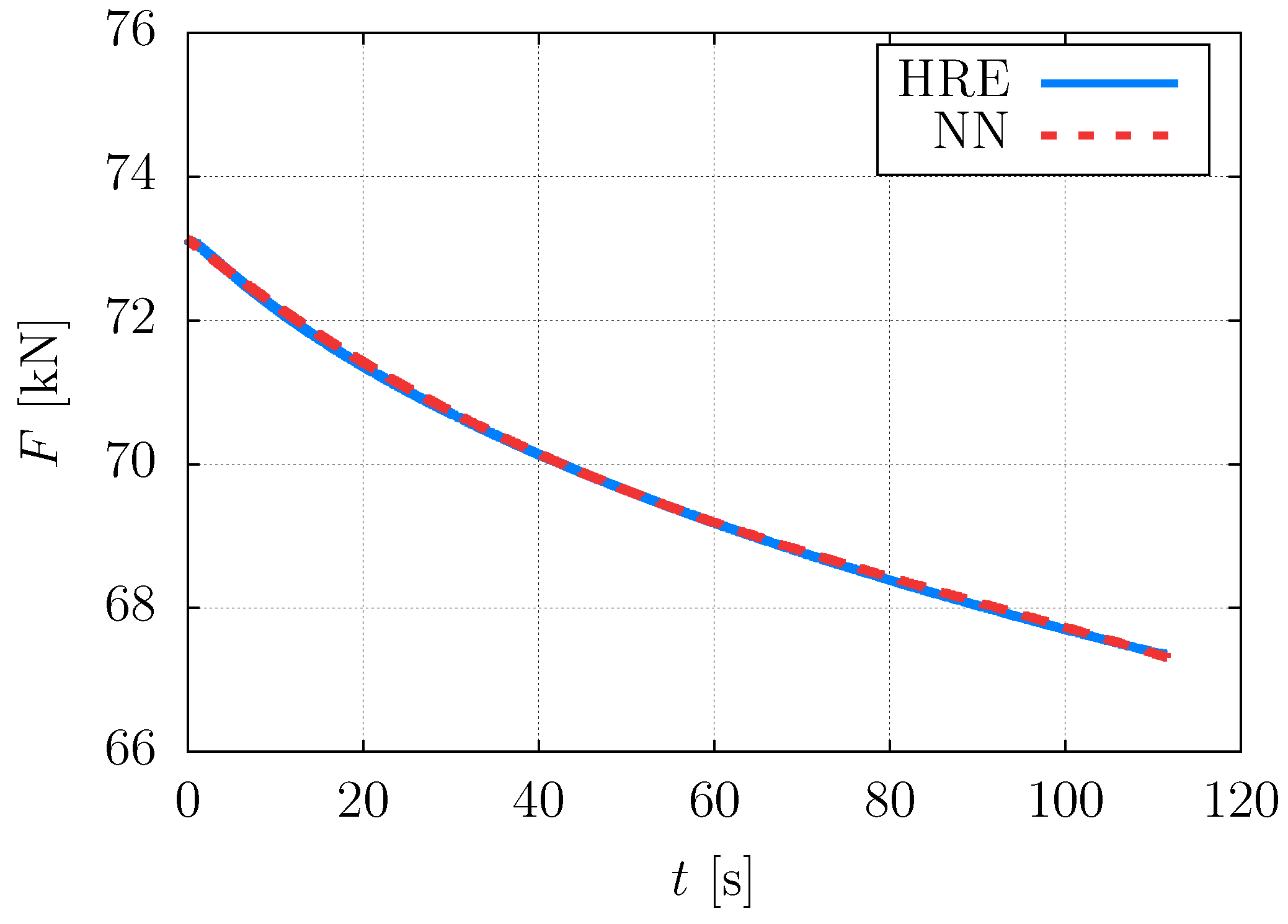
With the chosen network configuration, the prediction errors are small, with percentage errors of approximately $0.1\%$ for the main HRE performance quantities. In particular, the errors associated with the time-dependent quantities (thrust and mass flow rate), which are represented using cubic polynomial parametrizations, remain very small. Figure 12 compares the thrust curves computed with the HRE model and those reconstructed by the trained neural network for a representative engine configuration, showing that the two curves are nearly indistinguishable.

Such small errors in the HRE metrics are assumed to translate into payload ratio estimates with errors of the same order of magnitude.

Thus, a computationally efficient tool to be used within an optimization process is obtained. The initial training is the only computational cost associated with the use of the neural network, which has to be performed only once. On the other hand, the cost associated with the use of the trained network is comparable to a few matrix multiplications. The trained network can be used in the optimization process as many times as necessary, replacing the more computationally expensive physical model. Generating a training set of one million samples takes about 1 h with optimized code. When using the trained neural network, it takes approximately 10 min instead, resulting in a speedup factor of around six times. This speedup increases further with the complexity of the internal ballistics model. Note that the cost of building the database should not be used to directly compare the network-based and internal ballistics optimization approaches. Indeed, after the initial training, the network can be reused across multiple optimization runs without additional computational cost, yielding substantial savings. Moreover, the applicability of the surrogate model could also be extended to different scenarios within the same operational range of the HRE, making it a highly flexible tool. All the analyses shown in this section have been performed on a workstation equipped with an Intel^® Xeon^® W-2265 CPU with 24 parallel cores, running at a base clock speed of 3.50 GHz (1.2–4.8 GHz).

6.2. Integrated Optimization

The integrated optimization has been carried out for a three-stage modular launch vehicle with a 55-ton wet mass. A single pump-fed HRE unit is used, with the first, second, and third stages constituted by clusters of 16, 4, and 1 units, respectively. The optimal design of the single HRE unit ${\mathit{x}}_{\mathrm{HRE}}$ is searched for, along with the optimal LV thrust direction ${\mathit{x}}_{\mathrm{guide}}$ and flight parameters ${\mathit{x}}_{\mathrm{flight}}$. The final aim is to maximize the payload injection capability of the LV for a nominal mission targeting a 500 $\mathrm{k}$$\mathrm{m}$ polar circular orbit (Sun Synchronous Orbit, SSO). A relevant vehicle data are the fairing mass $m_{\mathrm{fairing}}=400\mathrm{kg}$. Inter-stage mass $m_{\mathrm{is}}$ can be computed with Equation (18), assuming a truncated cone shape with major and minor diameters equal to the connected stage diameters. The length of the inter-stage is computed as the minimal length required to cover the nozzle exit sections of the subsequent stage and at the same time to guarantee a connection angle lower than 30 degrees in order to reduce the LV drag coefficient.

Results of the optimization are shown in

Table 7. Optimum solution vector.

${\mathit{x}}_{\mathbf{flight}}$		${\mathit{x}}_{\mathbf{guide}}$		${\mathit{x}}_{\mathbf{HRE}}$
$t_{{\mathrm{b}}_{3,1}}$ [s]	100.0	${\theta }_{\mathrm{po}}$ [deg]	83.25	$L_{\mathrm{g}}$ [m]	2.82
$t_{c_3}$ [s]	679.3	${\psi }_{\mathrm{po}}$ [deg]	−2.49	$D_{\mathrm{c}}$ [m]	0.65
−		${\theta }_{{3,1}_i}$ [deg]	4.20	$D_{\mathrm{t},0}$ [m]	0.11
−		${\theta }_{{3,1}_f}$ [deg]	2.54	${\dot{m}}_{\mathrm{ox},0}$ [kg/s]	13.79
−		${\theta }_{{3,2}_i}$ [deg]	1.95	$D_{\mathrm{e},1}$ [m]	0.38
−		${\theta }_{{3,2}_f}$ [deg]	−0.92	$D_{\mathrm{e},2}$ [m]	1.25
−		−		$D_{\mathrm{e},3}$ [m]	1.64

, reporting the optimized design variables.

Table 8. Stages operating conditions.

	${\mathit{F}}_{\mathbf{vac}}^{\mathbf{max}}$ [kN]	$\overline{{\mathit{p}}_{\mathbf{c}}}$ [bar]	$\overline{\mathbf{O}/\mathbf{F}}$ [-]	$\overline{{\mathit{I}}_{\mathbf{sp}}}$ [s]	${\mathit{I}}_{\mathbf{tot}}$ [kN s]	${\mathit{t}}_{\mathbf{b}}$ [s]	${\mathit{k}}_{\mathbf{s}}$ [-]	${\mathit{k}}_{\mathbf{t}}$ [-]	${\mathit{k}}_{\mathbf{e}}$ [-]	${\mathit{L}}_{\mathbf{tot}}$ [m]	$\mathit{L}/\mathit{D}$ [-]
First, stage	1053.4	32.6	2.00	304.3	110,146.7	112.5	0.106	0.061	0.038	9.5	3.17
Second, stage	288.8	32.6	2.00	338.0	30,578.4	112.5	0.138	0.061	0.064	10.9	3.63
Third stage	73.1	32.6	2.00	342.9	7755.2	112.5	0.131	0.061	0.057	11.57	7.05

presents the operating conditions of the first, second, and third stages. Overlined quantities represent operating conditions averaged over the burn, and the specific impulse is measured in a vacuum. It should be noted that the optimized HRE units obtained in the present study exhibit $L/D$ ratios of approximately 7 (a single unit is represented by the $L/D$ ratio of the third stage), which lie well within the range identified by Dubey et al. [38] as suitable for maintaining the benefits associated with swirl injection before significant swirl decay occurs. In

Table 9. Stages mass budget.

	${\mathit{m}}_{\mathbf{ox}}$ [kg]	${\mathit{m}}_{\mathbf{fu}}$ [kg]	${\mathit{m}}_{\mathbf{c}}$ [kg]	${\mathit{m}}_{\mathbf{tk}}$ [kg]	${\mathit{m}}_{\mathbf{no}}$ [kg]	${\mathit{m}}_{\mathbf{ps}}$ [kg]	${\mathit{m}}_{\mathbf{tp}}$ [kg]	${\mathit{m}}_{\mathbf{ct}}$ [kg]	${\mathit{m}}_{\mathbf{sh}}$ [kg]	${\mathit{m}}_{\mathbf{anc}}$ [kg]	${\mathit{m}}_{\mathbf{is}}$ [kg]
First, stage	24,572.8	12,334.4	889.6	225.6	1185.6	17.6	267.2	1107.2	56	416.7	194
Second, stage	6143.2	3083.6	222.4	56.4	537.6	4.4	66.8	276.8	14	131.0	170
Third stage	1535.8	770.9	55.6	14.1	153.9	1.1	16.7	69.2	3.5	34.9	-

, the masses of the different subsystems are reported for each stage, with $m_{\mathrm{ps}}$ being the mass of the helium-based tank pressurization system, $m_{\mathrm{ct}}$ the mass of contingency reserves, and $m_{\mathrm{anc}}$ the mass of ancillary structures. Note that, although a mass of just 1.1 kg for the pressurization system may seem small, it is consistent with the use of a turbo-pump-fed system, which significantly reduces the tank pressure that needs to be maintained. Lastly,

Table 10. Launch vehicle velocity losses, propulsive $\mathrm{\Delta }v$, and mass budget.

$\mathbf{\Delta }{\mathit{v}}_{\mathbf{grav}}$ [m/s]	$\mathbf{\Delta }{\mathit{v}}_{\mathbf{aero}}$ [m/s]	$\mathbf{\Delta }{\mathit{v}}_{\mathbf{mis}}$ [m/s]	$\mathbf{\Delta }{\mathit{v}}_{\mathbf{pr}}$ [m/s]	${\mathit{m}}_{\mathbf{0}}$ [kg]	${\mathit{m}}_{\mathbf{u}}$ [kg]	$\mathit{\lambda }$ [-]
1319.9	302.0	937.6	9708.1	55,632	1003	0.018

reports the launch vehicle payload mass $m_{\mathrm{u}}$, the total velocity increment $\mathrm{\Delta }{v}_{\mathrm{pr}}$, and the cumulative gravitational $\mathrm{\Delta }{v}_{\mathrm{grav}}$, aerodynamic $\mathrm{\Delta }{v}_{\mathrm{aero}}$, and misalignment $\mathrm{\Delta }{v}_{\mathrm{mis}}$ losses.

Note that none of the optimized HRE parameters ${\mathit{x}}_{\mathrm{HRE}}$ resides at the boundaries of its design space, which suggests that further widening would not yield additional benefits.

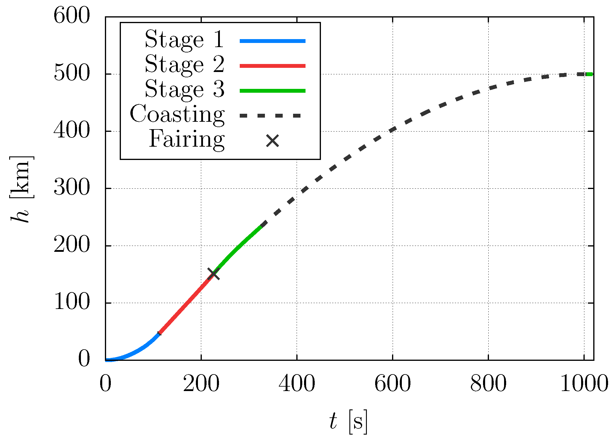
Figure 13 displays the altitude-time profile of the optimized flight trajectory. A direct ascent is flown. An altitude of approximately 151 km is reached at the end of the second stage cut-off, where the fairing is supposed to be jettisoned. The first burn of the third stage ends at an altitude of about 234 km. The acquired velocity of 7383.3 m/s is not sufficient to inject the LV into a Hohmann-like transfer orbit; rather, the optimization code suggests a shorter (ballistic) transfer arc with an apoapsis radius equal to the target orbit radius of 500 km. After this coasting phase, a brief reignition of the third stage of about ten seconds performs the injection into the final circular orbit. This direct ascent trajectory is possibly due to the relatively low altitude of the target orbit, as well as the low value of the velocity at the end of the first burn. Nevertheless, the restart capabilities of the HRE propulsion system are paramount to the success of the mission, allowing it to perform the circularization firing.

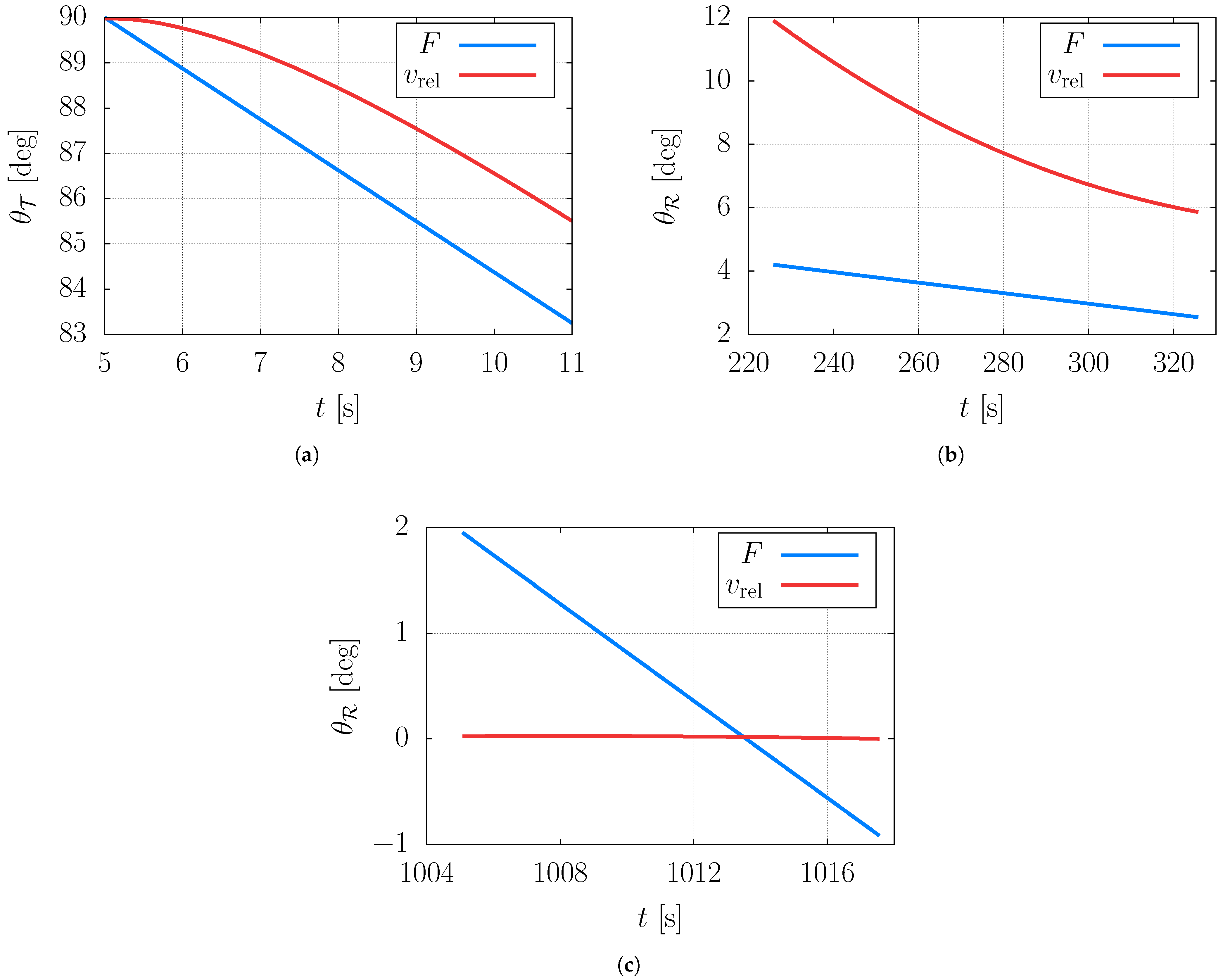
Figure 14 shows thrust elevation and flight path angle profiles during the pitch-over phase (Figure 14a, topocentric reference) and the two firings of the third stage (Figure 14b,c, RTN reference). The presence of a linear pitch law can be clearly seen in each figure, with the estimated aerodynamic angle of attack during pitch-over readily available as the difference between the two plotted curves. During orbit circularization (Figure 14c), velocity elevation approaches zero, as expected during a well-performed orbital injection.

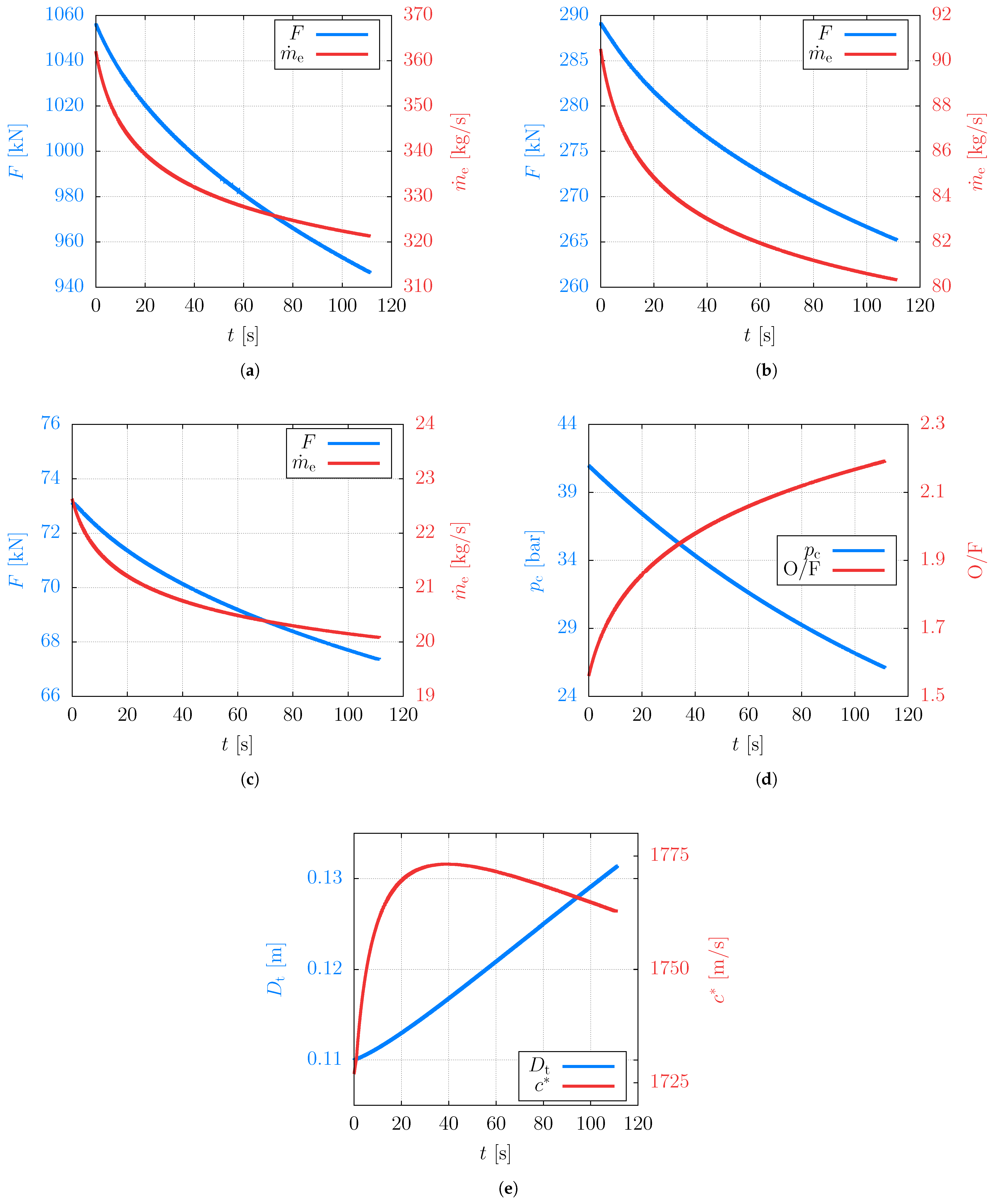
Figure 15 depicts the vacuum thrust and mass flow rate for each stage of the LV, along with the chamber pressure, mixture ratio, throat diameter, and characteristic velocity of the HRE unit. In these plots, typical patterns related to hybrid rockets can be seen. The reduction in ejected mass flow rate, thrust, and chamber pressure over time directly results from grain regression and throat erosion. Simultaneously, the increase in mixture ratio is characteristic of propellants with a mass flux coefficient n greater than 0.5. These trends are consistent with the expected behavior of hybrid rockets.

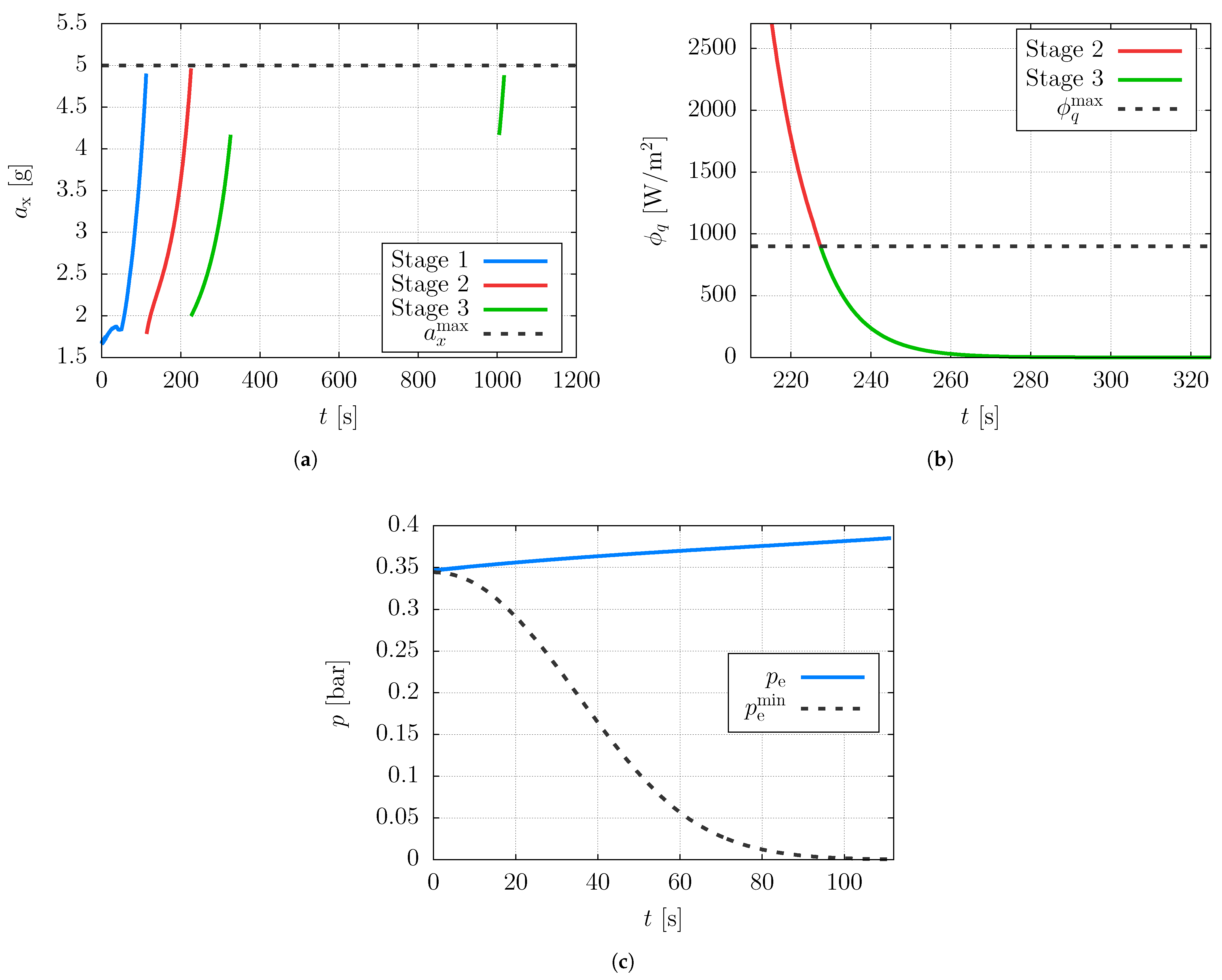
The dominant flight path constraints are shown in Figure 16. As expected, the optimal solution is attained with the LV operating at its maximum structural capabilities. Specifically, the longitudinal acceleration at cut-off of each stage is close to 5g (Figure 16a), which is the imposed limit. The fairing is jettisoned precisely once the payload heat flux exposure becomes acceptable (Figure 16b), and the first stage at lift-off operates with the nozzle flow at the boundaries of separation (Figure 16c). A noticeable “dip” in the first stage axial acceleration can be observed between 20 and 60 s in Figure 16a. This behavior is due to the launch vehicle experiencing its point of maximum aerodynamic drag around 50 s. After this point, as the drag rapidly decreases due to the reduction in air density with altitude, the increase in axial acceleration caused by the reduction of the vehicle mass related to propellant consumption becomes dominant.

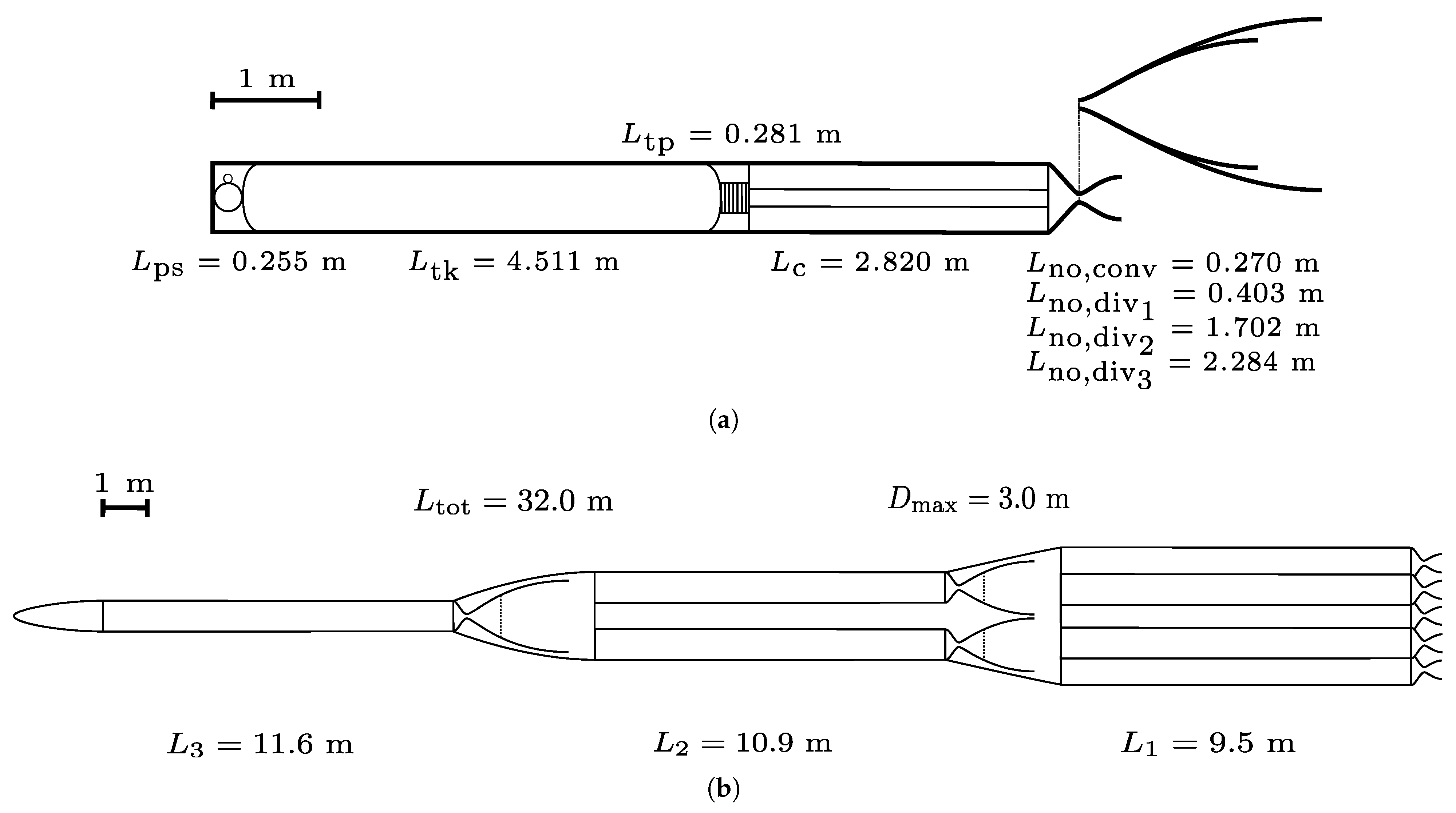
The optimized LV features a wet mass of 55 tons and a payload mass of 1003 kg ($\lambda =0.018$). It spans a length of 32.9 m, with a maximum diameter of 3 m, yielding a length-to-diameter ratio of $L/D=$10.97. When compared, for instance, to the early Vega C light [60] reference capabilities (a launch vehicle under development), which include a maximum payload mass of 300 kg with a gross mass of 55 tons ($\lambda =0.0055$) for roughly the same mission scenario, the HRE-based LV exhibits a remarkable enhancement in terms of payload ratio. This performance advantage can be mainly attributed to the higher specific impulse of HREs with respect to solid rockets, as well as HREs restart capabilities, enabling the execution of an efficient ascent trajectory. However, this is an overall comparison between two very different launchers, and it is based on the present analysis together with its assumptions; a more precise and accurate evaluation of the launch vehicle dry mass, combustion efficiency, and nozzle efficiency is warranted for obtaining a better estimate. In scale 2-D views of the optimized propulsion system are shown in Figure 17 for both the HRE unit (Figure 17a, with nozzle profiles for each of the three stages) and the entire LV (Figure 17b).

Note that such a high payload capacity of approximately 1000 kg is partially influenced by optimistic assumptions for parameters such as ${\eta }_{c^{*}}$ and ${\eta }_{C_F}$. Additionally, the second and third stages of the optimized launcher exhibit unusually high expansion ratios (130 and 220, respectively). These values result from optimistic assumptions in the nozzle mass estimation model, as well as the absence of cost constraints. Such large expansion ratios could also lead to reduced nozzle efficiencies due to increased losses, which have not been taken into account. To provide a less optimistic estimate of the LV performance, a simplified analysis was performed to evaluate the payload capacity of a launch vehicle using the same HRE units as the optimized configuration but with reduced efficiencies for ${\eta }_{c^{*}}$ and ${\eta }_{C_F}$, both set to 94%. The area ratios for the second and third stages were also reduced to 40 and 80 (shown in Figure 17b with black dotted lines), respectively, resulting in lighter nozzle and inter-stage masses. This analysis is based on Tsiolkovsky’s rocket equation, assuming a propulsive $\mathrm{\Delta }{v}_{\mathrm{pr}}$ equivalent to that of the optimized launcher (9.7 km/s). However, note that this approach does not account for the impact of such changes on velocity losses, which may further affect performance. Under these revised assumptions, the payload capacity drops to 662 kg, corresponding to a payload ratio of approximately $\lambda =0.012$. Note that the decrease in payload capacity is primarily due to the reduction in efficiencies, while the truncation of the nozzles had a rather marginal effect. This result provides a more conservative estimate of the propulsion system capabilities. Nonetheless, such a result still represents a noticeable improvement compared to the previously mentioned Vega C light reference capabilities.

7. Conclusions

In this study, an integrated optimization framework has been developed to determine the optimal hybrid rocket engine (HRE) design for a modular multistage launch vehicle targeting a 500 $\mathrm{k}$$\mathrm{m}$ polar circular orbit. A preliminary mission analysis based on Tsiolkovsky’s equation led to the selection of a three-stage launcher architecture, with stages composed of 16, 4, and 1 HRE units, respectively. To improve computational efficiency, a neural-network-based surrogate model was introduced to predict the performance of the reference HRE unit using data generated by a simplified 0-D internal ballistics model. A comprehensive parametric analysis of the training dataset size and network architecture was conducted, leading to the selection of a medium-sized network and dataset that balance predictive accuracy and computational effort. The resulting surrogate model accurately reproduces the HRE behavior, with errors of approximately 0.1% for key performance quantities. Due to the clustering approach, the same trained network can be used to estimate the performance of all stages. The use of the surrogate model provides a computational speedup of approximately six times with respect to the physics-based HRE model, while requiring training only once. The trained network can therefore be reused across multiple optimization runs and potentially extended to different mission scenarios within the same operational range. The integrated optimization results show that the proposed configuration can successfully accomplish the target mission. The optimized launcher features a wet mass of 55 tons and delivers a payload of 1003 kg ($\lambda =0.018$), demonstrating the feasibility of the proposed approach.

References

1. Wei, S.S.; Li, M.C.; Lai, A.; Chou, T.H.; Wu, J.S. A Review of Recent Developments in Hybrid Rocket Propulsion and Its Applications. Aerospace 2024, 11, 739. [Google Scholar] [CrossRef] [Scilit]
2. Aksen, U.; Aslan, A.R.; Goker, U.D. Comprehensive Six-Degrees-of-Freedom Trajectory Design and Optimization of a Launch Vehicle with a Hybrid Last Stage Using the PSO Algorithm. Appl. Sci. 2024, 14, 3891. [Google Scholar] [CrossRef] [Scilit]
3. Cai, G.; Zhu, H.; Rao, D.; Tian, H. Optimal Design of Hybrid Rocket Motor Powered Vehicle for Suborbital Flight. Aerosp. Sci. Technol. 2013, 25, 114–124. [Google Scholar] [CrossRef] [Scilit]
4. Quadros, F.D.A.; Lacava, P.T. Swirl Injection of Gaseous Oxygen in a Lab-Scale Paraffin Hybrid Rocket Motor. J. Propuls. Power 2019, 35, 896–905. [Google Scholar] [CrossRef] [Scilit]
5. Franco, M.; Barato, F.; Paccagnella, E.; Santi, M.; Battiston, A.; Comazzetto, A.; Pavarin, D. Regression Rate Design Tailoring Through Vortex Injection in Hybrid Rocket Motors. J. Spacecr. Rocket. 2020, 57, 278–290. [Google Scholar] [CrossRef] [Scilit]
6. Cai, G.; Zhao, Z.; Zhao, B.; Liu, Y.; Yu, N. Regression Rate and Combustion Performance Investigation on Hybrid Rocket Motor with Head-end Swirl Injection Under High Geometric Swirl Number. Aerosp. Sci. Technol. 2020, 103, 105922. [Google Scholar] [CrossRef] [Scilit]
7. Casalino, L.; Letizia, F.; Pastrone, D. Optimization of Hybrid Upper-Stage Motor with Coupled Evolutionary/Indirect Procedure. J. Propuls. Power 2014, 30, 1390–1398. [Google Scholar] [CrossRef] [Scilit]
8. Casalino, L.; Masseni, F.; Pastrone, D. Robust Design Approaches for Hybrid Rocket Upper Stage. J. Aerosp. Eng. 2019, 32. [Google Scholar] [CrossRef] [Scilit]
9. Casalino, L.; Masseni, F.; Pastrone, D. Deterministic and Robust Optimization of Hybrid Rocket Engines for Small Satellite Launchers. J. Spacecr. Rocket. 2021, 58, 1893–1903. [Google Scholar] [CrossRef] [Scilit]
10. Casalino, L.; Masseni, F.; Pastrone, D. Optimal Design of Electrically Fed Hybrid Mars Ascent Vehicle. Aerospace 2021, 8, 181. [Google Scholar] [CrossRef] [Scilit]
11. Casalino, L.; Masseni, F.; Pastrone, D. Optimal Design of Hybrid Rocket Small Satellite Launchers: Ground Versus Airborne Launch. J. Spacecr. Rocket. 2022, 59, 2084–2093. [Google Scholar] [CrossRef] [Scilit]
12. Messinger, T.L.; Corbiell, M.S.; Johansen, C.T. Optimization and Parametric Studies of Two-Stage-to-Orbit Liquid Oxygen/Paraffin Hybrid Rocket Vehicles. Aerosp. Sci. Technol. 2023, 140, 108495. [Google Scholar] [CrossRef] [Scilit]
13. Zhu, H.; Tian, H.; Cai, G.; Bao, W. Uncertainty Analysis and Design Optimization of Hybrid Rocket Motor Powered Vehicle for Suborbital Flight. Chin. J. Aeronaut. 2015, 28, 676–686. [Google Scholar] [CrossRef] [Scilit]
14. Pengcheng, W.; Hui, T.; Hao, Z.; Guobiao, C. Multi-Disciplinary Design Optimization with Fuzzy Uncertainties and its Application in Hybrid Rocket Motor Powered Launch Vehicle. Chin. J. Aeronaut. 2020, 33, 1454–1467. [Google Scholar] [CrossRef] [Scilit]
15. Zhu, H.; Xiao, M.; Zhang, J.; Cai, G. Uncertainty Design and Optimization of a Hybrid Rocket Motor with Mixed Random-Interval Uncertainties. Aerosp. Sci. Technol. 2022, 128, 107791. [Google Scholar] [CrossRef] [Scilit]
16. Zolla, P.; Rosa, R.; Migliorino, M.T.; Bianchi, D. Multi-disciplinary Optimization of Single-stage Hybrid Rocket with Swirl Injection for Lunar Ascent. In Proceedings of the AIAA SciTech Forum, National Harbor, MD, USA, 23–27 January 2023. AIAA Paper 2023-2349. [Google Scholar] [CrossRef] [Scilit]
17. Zolla, P.M.; Rosa, R.; Migliorino, M.T.; Bianchi, D. Multi-Disciplinary Optimization of Single-Stage Hybrid Rockets for Lunar Ascent. Acta Astronaut. 2024, 222, 493–507. [Google Scholar] [CrossRef] [Scilit]
18. Federici, L.; Zavoli, A.; Colasurdo, G.; Mancini, L.; Neri, A. Integrated Optimization of First-Stage SRM and Ascent Trajectory of Multistage Launch Vehicles. J. Spacecr. Rocket. 2021, 58, 786–797. [Google Scholar] [CrossRef] [Scilit]
19. Ampatzis, C.; Izzo, D. Machine Learning Techniques for Approximation of Objective Functions in Trajectory Optimisation. In Proceedings of the IJCAI-09 Workshop on Artificial Intelligence in Space, Pasadena, CA, USA, 17–18 July 2009. [Google Scholar]
20. Izzo, D.; Märtens, M.; Pan, B. A Survey on Artificial Intelligence Trends in Spacecraft Guidance Dynamics and Control. Astrodynamics 2019, 3, 287–299. [Google Scholar] [CrossRef] [Scilit]
21. Zavoli, A.; Federici, L. Reinforcement Learning for Robust Trajectory Design of Interplanetary Missions. J. Guid. Control. Dyn. 2021, 44, 1440–1453. [Google Scholar] [CrossRef] [Scilit]
22. Izzo, D.; Öztürk, E. Real-Time Guidance for Low-Thrust Transfers Using Deep Neural Networks. J. Guid. Control. Dyn. 2021, 44, 315–327. [Google Scholar] [CrossRef] [Scilit]
23. Shi, Y.; Wang, Z. Onboard Generation of Optimal Trajectories for Hypersonic Vehicles Using Deep Learning. J. Spacecr. Rocket. 2021, 58, 400–414. [Google Scholar] [CrossRef] [Scilit]
24. Scorsoglio, A.; Furfaro, R.; Linares, R.; Gaudet, B. Image-based Deep Reinforcement Learning for Autonomous Lunar Landing. In Proceedings of the AIAA SciTech Forum, Orlando, FL, USA, 6–10 January 2020. AIAA Paper 2020-1910. [Google Scholar] [CrossRef] [Scilit]
25. Song, Y.; Miao, X.; Cheng, L.; Gong, S. The Feasibility Criterion of Fuel-Optimal Planetary Landing Using Neural Networks. Aerosp. Sci. Technol. 2021, 116, 106860. [Google Scholar] [CrossRef] [Scilit]
26. Federici, L.; Benedikter, B.; Zavoli, A. Deep Learning Techniques for Autonomous Spacecraft Guidance During Proximity Operations. J. Spacecr. Rocket. 2021, 58, 1774–1785. [Google Scholar] [CrossRef] [Scilit]
27. Li, S.; Jiang, X. RBF Neural Network Based Second-Order Sliding Mode Guidance for Mars Entry Under Uncertainties. Aerosp. Sci. Technol. 2015, 43, 226–235. [Google Scholar] [CrossRef] [Scilit]
28. Zavoli, A.; Zolla, P.M.; Federici, L.; Migliorino, M.T.; Bianchi, D. Machine Learning Techniques for Flight Performance Prediction of Hybrid Rocket Engines. In Proceedings of the AIAA Propulsion and Energy Forum, Virtual Event, 9–11 August 2021. AIAA Paper 2021-3506. [Google Scholar] [CrossRef] [Scilit]
29. Zavoli, A.; Zolla, P.M.; Federici, L.; Migliorino, M.T.; Bianchi, D. Surrogate Neural Network for Rapid Flight Performance Evaluation of Hybrid Rocket Engines. J. Spacecr. Rocket. 2022, 59, 2003–2016. [Google Scholar] [CrossRef] [Scilit]
30. Zolla, P.M.; Zavoli, A.; Migliorino, M.T.; Bianchi, D. Surrogate Neural Network Model for Integrated Ascent Trajectory Optimization of Throttleable Hybrid Rockets. In Proceedings of the International Astronautical Congress, IAC, Baku, Azerbaijan, 2–6 October 2023. [Google Scholar]
31. Masseni, F. Towards the Integration of Surrogate Models in the Robust Optimization of Hybrid Rocket Engines. In Proceedings of the AIAA SciTech Forum, Orlando, FL, USA, 6–10 January 2025. AIAA Paper 20255-2786. [Google Scholar] [CrossRef] [Scilit]
32. Casalino, L.; Masseni, F.; Pastrone, D. Optimal Design Comparison of Hybrid Rocket for Small Satellite Launchers. In Proceedings of the AIAA Propulsion and Energy Forum, Virtual Event, 9–11 August 2021. AIAA Paper 2021-3505. [Google Scholar] [CrossRef] [Scilit]
33. Kanazaki, M.; Ito, S.; Kanamori, F.; Nakamiya, M.; Kitagawa, K.; Shimada, T. Design Optimization of Launch Vehicle Concept using Cluster Hybrid Rocket Engine for Future Space Transportation. J. Fluid Sci. Technol. 2016, 11, JFST0003. [Google Scholar] [CrossRef] [Scilit]
34. Wenzhi, H.; Hao, Z.; Wei, H.; Zhiguo, Z. Design Optimization of a Low-Cost Three-Stage Launch Vehicle with Modular Hybrid Rocket Motors. J. Phys. Conf. Ser. 2024, 2764, 012026. [Google Scholar] [CrossRef] [Scilit]
35. Tugnoli, M.; Sarret, M.; Aliberti, M. Overview on Micro Launchers. In European Access to Space: Business and Policy Perspectives on Micro Launchers; Springer International Publishing: Berlin/Heidelberg, Germany, 2019; pp. 5–28. [Google Scholar] [CrossRef] [Scilit]
36. Zolla, P.; Zavoli, A.; Migliorino, M.T.; Bianchi, D. Integrated Optimization of a Three-Stage Clustered Hybrid Rocket Launcher using Neural Networks. In Proceedings of the AIAA Scitech Forum, Orlando, FL, USA, 8–12 January 2024. AIAA Paper 2024-1184. [Google Scholar] [CrossRef] [Scilit]
37. Xia, H.; Wang, N.; Yang, J.; Wu, Y. Investigation of dynamic mixing combustion characteristics in variable thrust hybrid rocket motors. Combust. Flame 2023, 250, 112637. [Google Scholar] [CrossRef] [Scilit]
38. Dubey, A.; Kumar, R.; Biswas, S. Experimental studies on swirl injector with varying L/D ratio of hybrid rocket motor. Int. J. Heat Fluid Flow 2025, 112, 109734. [Google Scholar] [CrossRef] [Scilit]
39. Zolla, P.M.; Migliorino, M.; Bianchi, D.; Nasuti, F.; Pellegrini, R.; Cavallini, E. A Computational Tool for the Design of Hybrid Rockets. Aerotec. Missili Spaz. 2021, 100, 253–262. [Google Scholar] [CrossRef] [Scilit]
40. Veale, K.; Adali, S.; Pitot, J.; Brooks, M. A Review of the Performance and Structural Considerations of Paraffin Wax Hybrid Rocket Fuels with Additives. Acta Astronaut. 2017, 141, 196–208. [Google Scholar] [CrossRef] [Scilit]
41. Casalino, L.; Masseni, F.; Pastrone, D. Viability of an Electrically Driven Pump-Fed Hybrid Rocket for Small Launcher Upper Stages. Aerospace 2019, 6, 36. [Google Scholar] [CrossRef] [Scilit]
42. Karabeyoglu, M.A.; Zilliac, G.; Cantwell, B.J.; DeZilwa, S.; Castellucci, P. Scale-Up Tests of High Regression Rate Paraffin-Based Hybrid Rocket Fuels. J. Propuls. Power 2004, 20, 1037–1045. [Google Scholar] [CrossRef] [Scilit]
43. Gordon, S.; McBride, B.J. Computer Program for Calculation of Complex Chemical Equilibrium Compositions and Applications; Technical Report NASA-RP-1311; National Aeronautics and Space Admministration: Washington, DC, USA, 1996.
44. Pavli, A.J.; Kacynski, K.J.; Smith, T.A. Experimental Thrust Performance of a High-Area-Ratio Rocket Nozzle; Technical Report NASA-TP-2720; National Aeronautics and Space Admministration: Washington, DC, USA, 1987.
45. Stark, R. Flow Separation in Rocket Nozzles, a Simple Criteria. In Proceedings of the 41st AIAA/ASME/SAE/ASEE Joint Propulsion Conference & Exhibit, Tucson, AZ, USA, 10–13 July 2005. AIAA Paper 2005-3940. [Google Scholar] [CrossRef] [Scilit]
46. Bianchi, D.; Migliorino, M.T.; Rotondi, M.; Kamps, L.; Nagata, H. Numerical Analysis of Nozzle Erosion in Hybrid Rockets and Comparison with Experiments. J. Propuls. Power 2022, 38, 389–409. [Google Scholar] [CrossRef] [Scilit]
47. Bianchi, D.; Nasuti, F. Numerical Analysis of Nozzle Material Thermochemical Erosion in Hybrid Rocket Engines. J. Propuls. Power 2013, 29, 547–558. [Google Scholar] [CrossRef] [Scilit]
48. Migliorino, M.T.; Bianchi, D.; Nasuti, F. Graphite Nozzle Erosion Trends in Paraffin/Oxygen Hybrid Rockets. J. Propuls. Power 2022, 38, 508–522. [Google Scholar] [CrossRef] [Scilit]
49. Larson, W.J.; Henry, G.N.; Humble, R.W. Space Propulsion Analysis and Design; McGraw-Hill: New York City, NY, USA, 1995. [Google Scholar]
50. Saunders, D. A Method of Calculating the Weight and Dimensions of a Turbo Pump for Rocket Propellants; Technical Report R.P.D. 22; Royal Aircraft Establishment Farnborough: Farnborough, UK, 1949. [Google Scholar]
51. Frank, C.P.; Pinon-Fischer, O.J.; Mavris, D.N.; Tyl, C.M. Design Methodology for the Performance, Weight, and Economic Assessment of Chemical Rocket Engines. J. Aerosp. Eng. 2017, 30, 04016071. [Google Scholar] [CrossRef] [Scilit]
52. Morino, Y.; Shimoda, T.; Morimoto, T.; Ishikawa, T.; Aoki, T. Applicability of CFRP Materials to the Cryogenic Propellant Tank for Reusable Launch Vehicle (RLV). Adv. Compos. Mater. 2001, 10, 339–347. [Google Scholar] [CrossRef] [Scilit]
53. Glatt, C. WAATS: A Computer Program for Weights Analysis of Advanced Transportation Systems; Technical Report NASA-CR-2420; National Aeronautics and Space Administration: Washington, DC, USA, 1974.
54. Joseph, J.; Agrawal, G.; Agarwal, D.K.; Kumar, S.S. Analytical Study on Effect of Ullage Temperature and Helium Concentration on Cryogenic Tank Pressure During Sloshing. In Proceedings of the 25th National Symposium on Cryogenics, Hyderabad, India, 8–10 December 2014. [Google Scholar]
55. Aluminium/Aluminum 7050 Alloy (UNS A97050). Available online: https://www.azom.com/article.aspx?ArticleID=6650 (accessed on 1 March 2026).
56. Mechanical Properties of Carbon Fibre Composite Materials, Fibre/Epoxy Resin. Available online: http://www.performance-composites.com/carbonfibre/mechanicalproperties_2.asp (accessed on 1 March 2026).
57. Hornik, K.; Stinchcombe, M.; White, H. Universal Approximation of an Unknown Mapping and its Derivatives Using Multilayer Feedforward Networks. Neural Netw. 1990, 3, 551–560. [Google Scholar] [CrossRef] [Scilit]
58. Kingma, D.P.; Ba, J. Adam: A Method for Stochastic Optimization. arXiv 2014, arXiv:1412.6980. [Google Scholar]
59. NASA. US Standard Atmosphere; Technical Report NOAA-S/T-76-1562; National Oceanic and Atmospheric Administration: Washington, DC, USA, 1976.
60. Mancini, R.; Scardecchia, E.; Gallucci, S. Vega C Light, a Flexible and Low Cost Solution for Small Satellites. In Proceedings of the 8th European Conference for Aeronautics and Space Sciences (EUCASS), Madrid, Spain, 1–4 July 2019. [Google Scholar] [CrossRef]
61. Federici, L.; Benedikter, B.; Zavoli, A. EOS: A Parallel, Self-Adaptive, Multi-Population Evolutionary Algorithm for Constrained Global Optimization. In Proceedings of the IEEE Congress on Evolutionary Computation (CEC), Glasgow, UK, 19–24 July 2020. [Google Scholar] [CrossRef] [Scilit]
62. Federici, L.; Zavoli, A.; Colasurdo, G. Evolutionary Optimization of Multirendezvous Impulsive Trajectories. Int. J. Aerosp. Eng. 2021, 2021, 9921555. [Google Scholar] [CrossRef] [Scilit]
63. Federici, L.; Zavoli, A.; Colasurdo, G. Preliminary Capture Trajectory Design for Europa Tomography Probe. Int. J. Aerosp. Eng. 2018, 2018, 6890173. [Google Scholar] [CrossRef] [Scilit]
Figure 1. Hybrid rocket design parameters.
Aerospace 13 00374 g001
Figure 2. Neural network surrogate model for HRE performance prediction.
Aerospace 13 00374 g002
Figure 3. Payload ratio behavior with respect to the number of stages using Tsiolkovsky’s equation.
Aerospace 13 00374 g003
Figure 4. Clusters of HRE units (not to scale). (a) First, stage. (b) Second, stage.
Aerospace 13 00374 g004
Figure 5. Reference frames. (a) Topocentric reference frame. (b) Radial-traverse-normal reference frame.
Aerospace 13 00374 g005
Figure 6. Phases of the optimal control problem (time not to scale). In the figure, the number in parentheses indicates the stage currently firing. Black dots mark the points at which a stage is ignited, while white dots indicate the points at which a stage is shut down. Each segment represents a specific maneuver, listed together with the control parameters used to describe it.
Aerospace 13 00374 g006
Figure 7. Flowchart of the integrated optimization procedure.
Aerospace 13 00374 g007
Figure 8. Evolution of the surrogate neural network errors with the training epoch (Net4, 500k training samples).
Aerospace 13 00374 g008
Figure 9. MSE and MAE F of the trained network with respect to the dimensions of the training datasets and for different network architectures. (a) MSE. (b) MAE F .
Aerospace 13 00374 g009
Figure 10. MSE and MAE F of the trained network with respect to the network architecture and for different training datasets. (a) MSE. (b) MAE F .
Aerospace 13 00374 g010
Figure 11. Training CPU time for different training dataset dimensions and network architectures.
Aerospace 13 00374 g011
Figure 12. Comparison between a true thrust curve provided by the HRE model and the corresponding prediction from the neural network.
Aerospace 13 00374 g012
Figure 13. Ascent trajectory profile of the optimized launcher.
Aerospace 13 00374 g013
Figure 14. Thrust elevation and flight path angle during pitch-over and upper stage operation phases. (a) Pitch-over. (b) First, upper stage burn. (c) Orbit insertion.
Aerospace 13 00374 g014
Figure 15. HRE performance parameters. (a) First, stage vacuum thrust and mass flow rate. (b) Second, stage vacuum thrust and mass flow rate. (c) Third stage vacuum thrust and mass flow rate. (d) HRE unit chamber pressure and mixture ratio. (e) HRE unit throat diameter and characteristic velocity.
Aerospace 13 00374 g015
Figure 16. Flight path constraints in the optimal solution. (a) Axial acceleration during the launch vehicle flight. (b) Payload heat flux exposure during second and third stage flight. (c) Nozzle exit pressure during first stage flight.
Aerospace 13 00374 g016
Figure 17. In-scale 2D views of the optimized propulsion system. (a) HRE unit. (b) Launch vehicle (nozzle truncation with black-dotted lines).
Aerospace 13 00374 g017