


Abstract
In active debris removal missions in low Earth orbit, the semi-major axis difference between a service platform and its target can be large. Analytical relative dynamics models used in formation-flying applications typically retain only the first-order expansion in the orbital element differences; at large separations, the discarded higher-order terms—particularly the power-law dependence on the semi-major axis—introduce systematic along-track drift that degrades the propagation accuracy. This paper derives the power-law truncation correction, a closed-form additive vector that exactly compensates the truncated semi-major-axis power-law remainder, together with a consistent Jacobian correction for the extended Kalman filter covariance prediction. The state dimension and state transition matrix structure remain unchanged. Propagation tests over semi-major axis differences of 36–146 km yield ten-revolution terminal position errors of 0.008–0.065 km for the corrected models, compared with tens to hundreds of kilometers for the uncorrected first-order models and 0.1–8 km for the second-order state transition tensor. In 500-run Monte Carlo angles-only filtering experiments, the corrected filter reduces the median terminal position error by one to nearly three orders of magnitude relative to the uncorrected model. A process noise sensitivity study confirms robustness to calibration uncertainty across two orders of magnitude at a lower computational cost and with simpler implementation than higher-order tensor methods.
1. Introduction
The ongoing accumulation of space debris in low Earth orbit (LEO) poses a growing collision risk to operational satellites. As of 2024, space surveillance networks catalog approximately 40,000 objects in Earth orbit, while debris environment models estimate over one million objects larger than 1 cm [1,2]; events such as the 2021 Cosmos 1408 anti-satellite test have further accelerated this growth [3]. The highest spatial density of cataloged debris is concentrated in the 700–1000 km altitude zone [4], a region that also hosts the largest population of Earth observation and sun-synchronous satellites and is therefore a priority region for active debris removal (ADR) [5,6]. Traditional ADR missions target large cataloged objects such as defunct satellites and spent upper stages through dedicated rendezvous and capture operations [7,8]. The far larger population of small (1–10 cm) debris, however, numbers in the millions, is largely uncatalogued, and carries no prior orbital information, rendering individual rendezvous manoeuvres impractical and demanding a fundamentally different removal strategy. Non-contact removal concepts such as laser ablation from a service platform deployed in a debris-dense orbital band [9,10] address this challenge by keeping the platform in its operational orbit while debris at various altitudes within the band drifts through the effective operating range. Operating such a platform requires autonomous detection and the tracking of each target by an onboard optical sensor, followed by orbit determination from angles-only measurements, target assessment, collision risk assessment, and laser irradiation scheduling—all of which depend on accurate relative orbit propagation. Because the platform remains in its operational orbit while debris objects populate a range of altitudes across the band, the semi-major axis difference () between the platform and target typically spans tens to hundreds of kilometers, making large the prevailing operational condition.
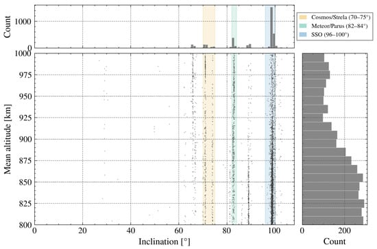
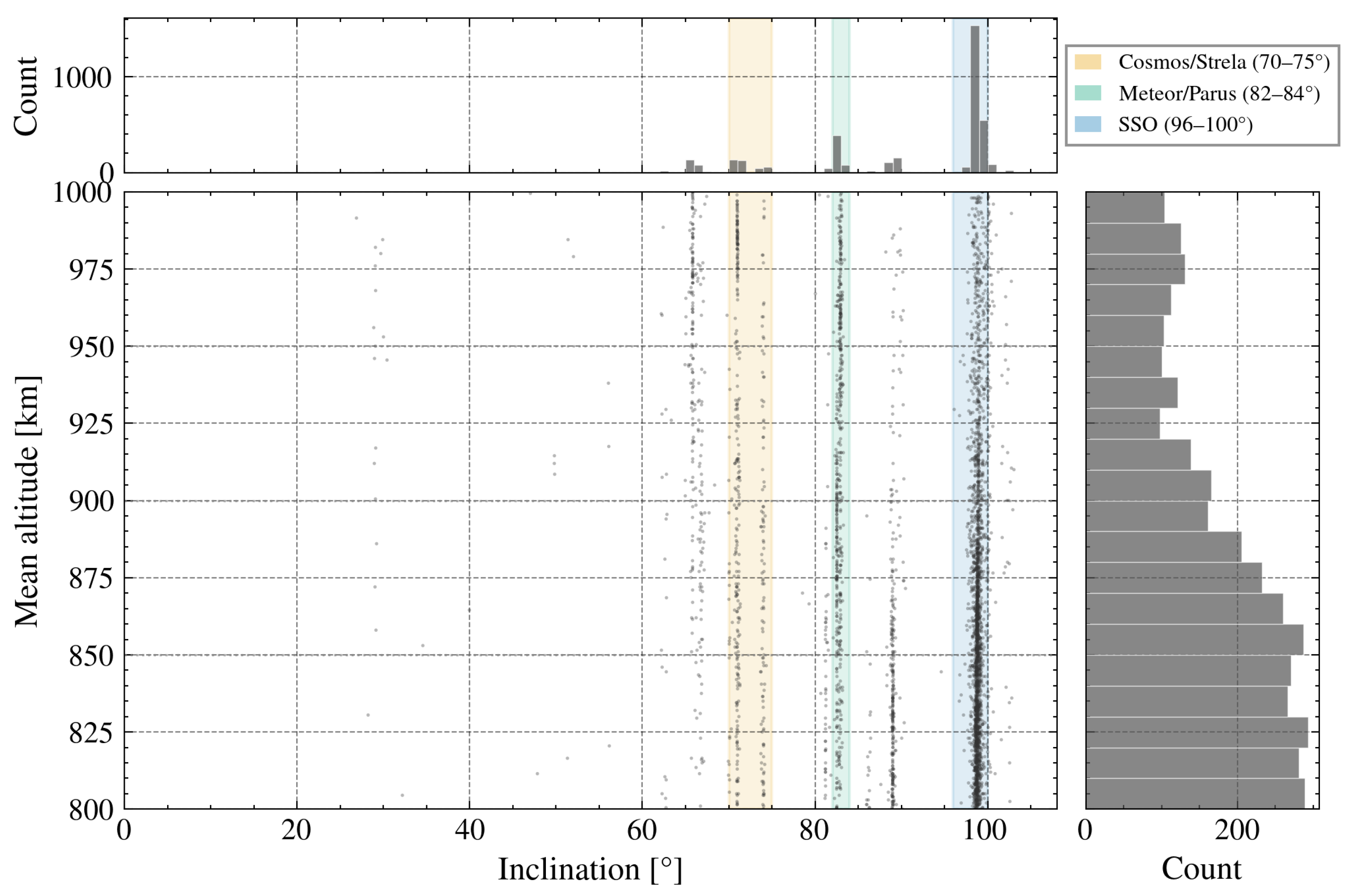
To quantify the magnitude of this separation, the CelesTrak Satellite Catalog (SATCAT) on-orbit debris database [11] was queried (filter: NAME=DEB; ONORBIT=1) for objects in the 800–1000 km altitude shell. Figure 1 shows the joint altitude–inclination distribution of N = 3742 cataloged debris objects in this shell. The Cosmos/Strela debris family near , the Meteor/Parus constellation debris near , and the dominant sun-synchronous orbit (SSO) band near form three distinct inclination clusters. The cataloged population (>10 cm) shown here represents a fraction of the total; the 1–10 cm population is estimated to be 10–100× denser (ESA MASTER model [2]), implying a substantially denser encounter environment for a service platform.
Figure 1.
Altitude–inclination distribution of cataloged debris in the 800–1000 km shell (CelesTrak SATCAT). Each point represents one cataloged object (N = 3742); shaded bands highlight three inclination clusters; and dashed lines mark platform altitudes at 850, 900, and 950 km. Marginal histograms show the one-dimensional projections.
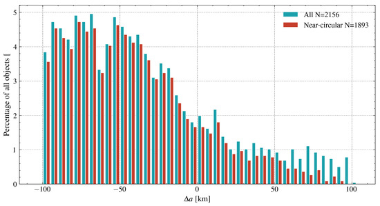
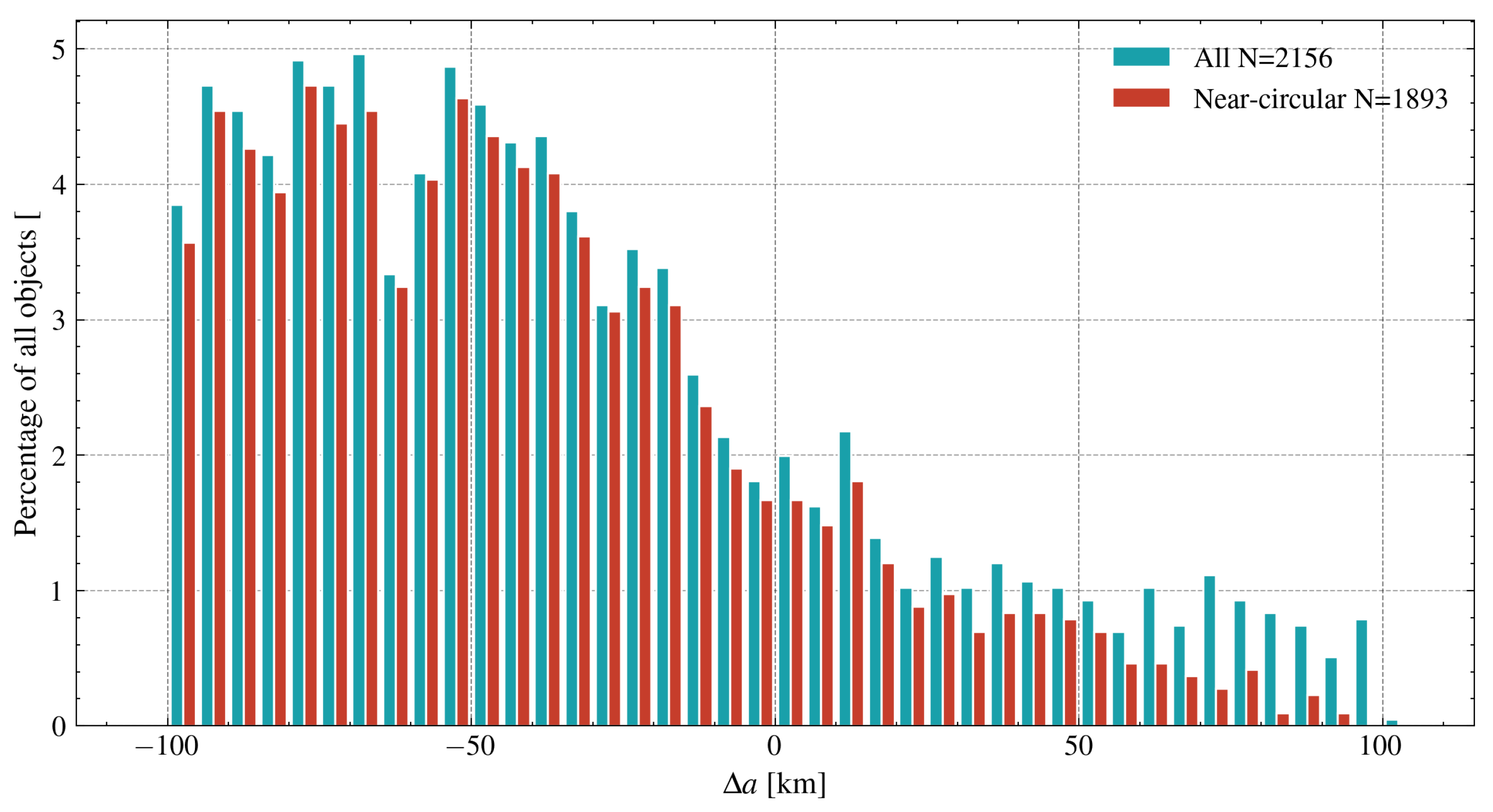
Figure 2 shows the distribution for the SSO band relative to a 900 km platform (N = 2156), for which the median is km and only 17.3% of the targets satisfy km. A sensitivity analysis across three platform altitudes (850, 900, and 950 km) and all three inclination clusters confirms that the fraction of targets with km exceeds 65% in every combination and reaches 92% in the worst case, demonstrating that large is a pervasive feature of the debris environment independent of the specific platform altitude or inclination selection.
Figure 2.
Distribution of the semi-major axis difference of cataloged debris relative to a 900 km service platform in the sun-synchronous orbit band (), altitude range 800–1000 km (CelesTrak SATCAT, query date 13 February 2026).
The onboard optical sensor provides azimuth and elevation measurements of the target relative to the platform, so a relative state estimation framework is the natural choice. In a mean element formulation, the relative orbital element (ROE) parametrization separates secular drift from periodic relative motion and places the along-track drift rate under the direct control of the dimensionless relative semi-major axis, which simplifies process model design and filter tuning. The relative dynamics are propagated through a first-order Taylor expansion of the secular rates with respect to the chief orbital elements, yielding a closed-form state transition matrix (STM). Although first-order STMs—including those that admit unbounded separations [12,13]—have been successfully applied in close formation-flying regimes, the underlying first-order linearization of the secular rates truncates the power-law dependence of mean motion and precession rates. At ADR scales where spans tens to hundreds of kilometers, this truncation biases the secular drift rates, and the resulting along-track phase error grows linearly with the propagation interval. Because this truncation error is deterministic rather than stochastic, it cannot be absorbed through process noise tuning. Periodic observation gaps caused by illumination constraints, sensor field-of-view (FOV) limitations, and unfavourable relative geometry [14] further aggravate the problem, as the filter coasts on the process model alone during each gap and truncation drift accumulates without correction. Accurate relative orbit propagation at a large is therefore essential for reliable relative state estimation in this operational regime.
The ROE parametrization—defined as the functional difference between the orbital elements of two spacecraft—derives from the eccentricity/inclination vector separation technique developed for geostationary Earth orbit (GEO) co-location [15] and subsequently adapted to LEO formation flying by D’Amico and Montenbruck [16] and D’Amico [17]. This parametrization has since become widespread in formation-flying guidance, navigation, and control (GNC) algorithm development [18,19,20]. A family of first-order STMs has been derived by differentiating the secular rates of the mean elements with respect to the chief orbit and integrating the resulting variational equation to obtain a closed-form matrix. D’Amico [17] derived a near-circular, bounded-separation STM; Gaias et al. [12] extended this to unbounded separations; Koenig et al. [13] generalized the formulation to eccentric reference orbits while retaining the first-order linearization; and the Gim–Alfriend STM [21,22] provides an equivalent first-order description in a different element set. Sullivan et al. [23,24] demonstrated that the effect of process model accuracy on filter performance exceeds the difference between filter architectures (extended Kalman filter, EKF, versus unscented Kalman filter, UKF), even at the moderate separations typical of formation flying. The first-order STM has been applied in multi-satellite swarm control [20], autonomous angles-only relative navigation [24,25], and the NASA Starling four-satellite formation flying experiment [19]. All members of this family, however, share the same structural limitation: the secular rates are linearized to first order in the orbital element differences, which truncates the power-law terms responsible for along-track drift at large separations.
An alternative derivation path starts from the Brouwer secular solution for the mean elements, differentiates the resulting closed-form expressions to obtain the STM and state transition tensor (STT), and is in principle extensible to any order. Gaias, Colombo, and Lara [26] developed a comprehensive ROE framework along this path, providing a first-order STM that includes – zonal harmonics together with a second-order STT and second-order mean-to-osculating transformation; Guffanti and D’Amico [27] extended the Gim–Alfriend geometric method to incorporate solar radiation pressure (SRP) in a completely non-singular element set, thereby broadening linear relative-motion modeling to SRP-perturbed scenarios. Yang and collaborators [14,28] derived second-order state transition tensors for -perturbed relative motion and applied them to an analytical second-order EKF for angles-only estimation. Willis et al. [29] obtained a closed-form second-order solution for relative motion in the two-body problem; while effective for short-arc Keplerian propagation, the omission of secular precession limits its applicability to multi-revolution -dominated LEO scenarios. Higher-order methods reduce truncation error by retaining additional Taylor terms at the expense of Hessian computation and tensor contraction. For large semi-major-axis separations, the first-order truncation error becomes substantial, and the second-order correction still leaves a residual that accumulates over multiple orbits. The power-law structure can, however, be evaluated exactly without Taylor expansion, yielding a closed-form correction to the dominant truncation term at negligible computational cost.
Adaptive filtering techniques such as online process noise estimation [30,31] can increase the tolerance of random process model errors but cannot remove the systematic bias introduced by the truncation of the state space model. Inflating the process noise covariance Q absorbs part of the drift and widens the estimated covariance, yet it does not address the root cause and creates a disparity between the estimated and actual covariance. Data-driven methods such as neural network-based orbit uncertainty propagation [32] and machine learning-based orbit prediction [33] can adapt to complex perturbation environments but require training data and do not preserve the closed-form STM structure required for onboard real-time evaluation.
This paper develops a power-law truncation correction (PLTC) for first-order ROE-STMs. The method constructs a closed-form additive compensation vector from the exact remainder of the truncated power-law expansion, thereby exactly compensating the truncated semi-major-axis power-law remainder and leaving the state dimension and STM structure unchanged. A consistent Jacobian correction maintains alignment between the compensated process model and the EKF covariance prediction. The correction is derived in a general form applicable to first-order STMs whose secular rates exhibit scaling, and is instantiated and validated within Gaias et al.’s [26] first-order framework, where it is compared with the Gaias second-order STT through propagation experiments and 500-trial Monte Carlo (MC) angles-only EKF simulations.
The remainder of this paper is organized as follows. Section 2 presents the general even-zonal relative dynamics model, the PLTC derivation with the formulation as a special case, and the EKF integration. Section 3 reports the propagation accuracy, Monte Carlo filtering performance, computational cost, and applicability boundaries. Section 4 summarizes the conclusions and outlines future work.
2. Method
This section develops the power-law truncation correction (PLTC) on the first-order mean-ROE framework of Gaias et al. [26]. The key observation is that, in the ADR regime considered here, the dominant deterministic error is not distributed uniformly across the STM, but is concentrated in the semi-major-axis truncation embedded in its first column. We therefore begin from the general even-zonal form of the Gaias secular solution, isolate the associated power-law remainder, and recast it as a closed-form additive correction that preserves the original state dimension and sparsity pattern. The model used in the numerical experiments then appears as a special case of the same construction; in that limit, the explicit Gaias STM is algebraically equivalent to the secular ROE STM of Koenig et al. [13]. The resulting compensated process model is embedded in an EKF without altering the nonlinear observation chain.
2.1. Relative Dynamics Model
The process model is formulated in the mean non-singular element set
where a is the semi-major axis, u is the mean argument of latitude, are the components of the eccentricity vector, i is the inclination, and is the right ascension of the ascending node. The EKF state is the mean relative orbital element vector
with denoting deputy-minus-chief differences. This parametrization is inherited directly from the ROE definition adopted by Gaias et al. [26]; it is non-singular for the near-circular LEO regime of interest and keeps the in-plane/out-of-plane coupling under tighter control than formulations based on the true argument of latitude.
After osculating-to-mean conversion, the conservative mean dynamics preserve a and i, so the secular motion is carried only by , M, and . Gaias et al. show that the chief mean orbit can therefore be written in closed form as [26]
where and . Each secular rate is the sum of retained zonal contributions,
with and denoting the Keplerian term. This form is more than a compact rewriting of the secular solution: it makes the geometry of the STM explicit. The mean eccentricity vector undergoes a planar rotation driven by the accumulated apsidal precession, while the longitudinal variables drift linearly at the sum of the secular angular rates.
A first-order expansion of Equation (3) with respect to the initial chief mean elements yields the ROE state transition matrix
where the full closed-form first-order mean-ROE STM is given by Gaias et al. [26]. Since PLTC acts only on the semi-major-axis truncation embedded in column 1, we write that column explicitly as
where
Equation (5) is the first-order ROE propagation law based on the STM of Gaias et al. [26]. When is restricted to , the full matrix reduces to the explicit form given by Gaias et al. [26]; that matrix is algebraically equivalent to the Koenig secular ROE STM, so the distinction between the two formulations is one of derivation and notation rather than underlying dynamics.
The structure that matters for PLTC is concentrated in the explicit first column . For any long-term rate , each zonal contribution may be written as
with , , , and . Equation (6) therefore represents a first-order approximation of exact power-law changes in a, whereas the remaining columns of arise from polynomial and trigonometric sensitivities in , , and i. In the ADR regime considered here, where is orders of magnitude larger than the other ROE components, this asymmetry makes the semi-major-axis truncation the dominant deterministic error source.
2.2. Power-Law Truncation Correction
Let the deputy semi-major axis at the initial epoch be . For the generic power-law contribution of Equation (8), the exact rate difference generated by the semi-major-axis offset alone is
where the subscript 0 denotes evaluation at the chief mean orbit . The first-order STM does not retain this exact change. Instead, it replaces it with the local tangent . The discrepancy is not stochastic, nor is it a high-order detail that remains uniformly small under propagation: because the secular rates integrate over time, the discarded remainder accumulates coherently into longitudinal drift.
The compensation follows from a single identity. Define the power-law remainder
and its derivative
then
The first term on the right-hand side is exactly the contribution already present in the -dependent entries of Equation (6); the second is the closed-form part discarded by linearization. Equation (12) makes the logic of PLTC precise: the method does not alter the baseline STM, but appends the missing remainder as an additive state correction. Because
the compensation is second order in the local limit and vanishes smoothly as .
The compensated propagation law in the general even-zonal case is therefore written as
with
Only the driven channels receive a correction. The conserved channels remain untouched, which preserves both the state dimension and the sparsity pattern of the original STM. The baseline first-order transport remains intact, while a closed-form nonlinear correction is added only through the semi-major-axis remainder that was truncated by the first-order expansion. The compensation is exact for that truncated power-law remainder, whereas residual mixed nonlinearities associated with phase rotation and cross-channel coupling remain represented at the baseline first-order level.
The special case used in the numerical experiments follows immediately by restricting to . Define
Then the relevant secular rates are
so that
The asymmetry across the channels is worth stressing. In the special case, is driven by two distinct exponents: m = 3/2 from the Keplerian mean motion and from the secular rates. By contrast, involve only the m = 7/2 remainder. Because the explicit Gaias matrix is equivalent to the Koenig STM, Equation (18) is also the correction to be applied when the baseline is implemented in Koenig notation.
The scale of the remainder in the special case is summarized in Table 1. The tabulated values are not introduced as a surrogate for the derivation; rather, they quantify a point that the algebra already implies. Although exceeds at fixed , the induced drift in is dominated by the Keplerian part because is much larger than . In practice, it is the mismatch in mean motion, not the precession correction, that sets the scale of the uncompensated along-track error.
Table 1.
Remainder values and their contributions to the along-track drift in the special case used in this study (ten-revolution propagation; km).
2.3. Integration of PLTC with the EKF
The filter state is the mean ROE vector . For a discrete propagation interval , the general even-zonal prediction step is written as
where and the secular rates inside are evaluated at the chief mean orbit at the previous epoch. This ordering matters. The STM and the compensation are evaluated from the same chief mean orbit and therefore use the same secular rate set consistently. In that way the compensation does not become an external bias term, but remains embedded in the same dynamical skeleton as the baseline propagation.
Because depends only on the first state component, the Jacobian correction is rank one. Differentiating Equation (15) with respect to results in
where . The corrected state transition Jacobian is therefore
with . The covariance prediction remains in standard EKF form,
but the role of Q changes materially: once the deterministic semi-major-axis truncation is removed from the process model, Q no longer needs to absorb a secular bias masquerading as stochastic uncertainty.
For the special case, Equation (20) reduces to
The Koenig and Koenig + PLTC methods reported in Section 3 instantiate the process model in this form; the Gaias-framework methods (first-order, second-order, and Gaias + PLTC) use the general even-zonal form of Equation (15) with .
The observation model is left untouched by PLTC. The sensor is a body-fixed optical camera on the servicing platform that measures azimuth and the elevation of the target in the chief radial–transversal–normal (RTN) frame, providing a bearing but no range (angles-only navigation). Given the predicted mean ROE state and the chief mean elements, the deputy mean elements are reconstructed directly from Equation (2) as
Both the mean element sets are then converted to osculating elements using the second-order KA- transformation of Gaias et al. [26],
so that the measurement model remains dynamically consistent with the mean-state process model. The inverse (osculating to mean) is obtained by traversing the three Lie-series layers in reverse order, yielding a direct analytical computation without iteration [26]. From the osculating elements, Kepler’s equation is solved to obtain the true anomaly from the mean anomaly, and the inertial positions then follow from the standard conic-section relations. The relative displacement is projected into the chief RTN frame as
with , , and . The sensor observables are azimuth and elevation,
and the measurement Jacobian is computed by forward finite differences of the full nonlinear observation chain,
following the same philosophy adopted in recent angles-only ROE navigation studies [23,25]. The update step is then the standard EKF correction. PLTC enters only through Equations (19)–(22); the measurement model, Kalman gain, and covariance update remain unchanged. This separation is operationally useful, because it confines the methodological modification to the prediction block while preserving the existing measurement-processing pipeline.
3. Results and Discussion
The preceding analysis shows that PLTC eliminates the dominant truncation drift in open-loop propagation; the question remains whether this improvement persists in a closed-loop filter where process noise, measurement noise, and covariance dynamics interact. To address this, propagation errors for five analytical methods (Koenig, Koenig + PLTC, Gaias first-order, Gaias second-order, and Gaias + PLTC) are first compared against matched truth models (Section 3.2); the three Gaias-framework methods are then tested in 500-trial Monte Carlo EKF experiments under three observation schedules (Section 3.3).
3.1. Simulation Configuration
Table 2 lists the platform orbit, truth model settings, and sensor parameters. Reference trajectories are generated with matched truth models: for the Koenig and Koenig + PLTC methods, a analytical propagator provides the truth; for the Gaias, Gaias (second), and Gaias + PLTC methods, a matched even-zonal propagator including the secular effects of , , , and serves as the truth. This matched truth approach isolates the truncation error inherent in each STM framework from force-model mismatch. The measurement noise covariance is with . All simulations were implemented in Python 3.11 with NumPy 1.26.
Table 2.
Common simulation parameters.
The process noise covariance Q for each analytical model is set to , where ⊙ denotes the element-wise product and is the one-step prediction residual against the matched truth, evaluated at the mixed-ROE initial condition of Table 3. The residual captures both stochastic perturbations and any deterministic truncation drift. This truth-based calibration represents a best case; Section 3.3.6 tests the sensitivity to Q mistuning. The calibrated diagonals are
Table 3.
Validation scenario definitions.
The initial error covariance is the same for all methods and uses the full matrix estimated for the mixed-ROE initialization, with diagonal entries . It also contains strong in-plane correlations (, , and ) and nearly decoupled out-of-plane channels. At the initial epoch (), this corresponds to equivalent RTN position standard deviations of m.
Table 3 defines the test scenarios. Propagation scenarios P1–P2 compare the model-only errors of five methods (two -framework: Koenig and Koenig + PLTC; three zonal-framework: Gaias first-order, Gaias second-order, and Gaias + PLTC); filtering scenarios F1–F3 compare the three Gaias-framework methods (Gaias first-order, Gaias second-order, and Gaias + PLTC). Each filtering scenario runs N = 500 Monte Carlo trials with initial states drawn by Latin Hypercube Sampling (LHS) from . The inverse normal cumulative distribution function (CDF) is applied to each marginal to preserve the Gaussian distribution while achieving more uniform coverage of the six-dimensional state space than standard random sampling at the same N. Because LHS introduces inter-sample stratification, the confidence bands used in the normalized estimation error squared (NEES) and normalized innovation squared (NIS) tests are treated as approximate diagnostic references rather than exact hypothesis test thresholds. Identical random sequences are used for all methods. The simulation spans 3 h at a 10 s sampling interval. Additional propagation sensitivity sweeps (eccentricity, inclination, and force–model mismatch) supporting the applicability analysis are described in Section 3.5.
3.2. Propagation Accuracy Comparison
3.2.1. Sweep (Scenario P1)
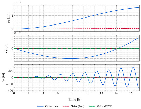
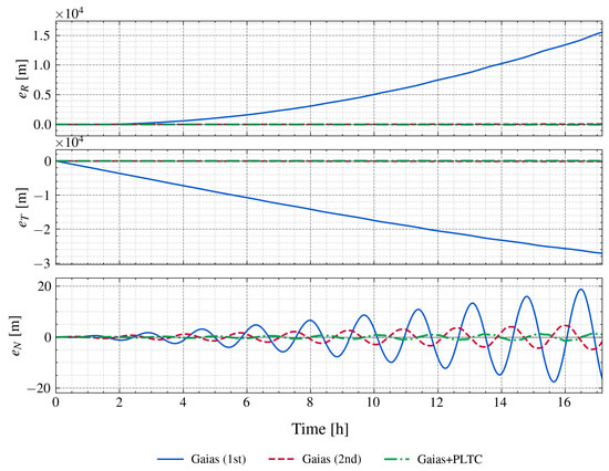
Scenario P1 sets the true initial state to and sweeps ( 36–146 km), thereby isolating the influence of the semi-major axis difference on the truncation error and allowing for direct comparison with the prediction of Section 2.1.
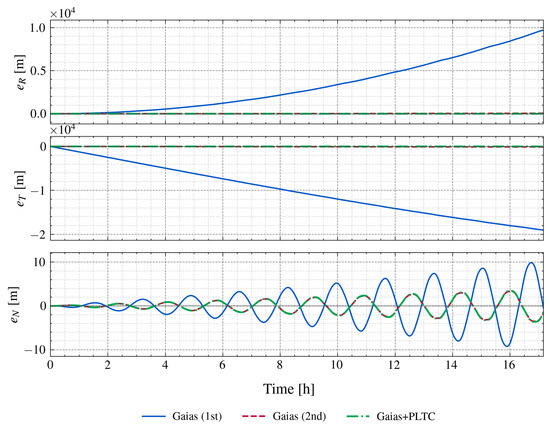
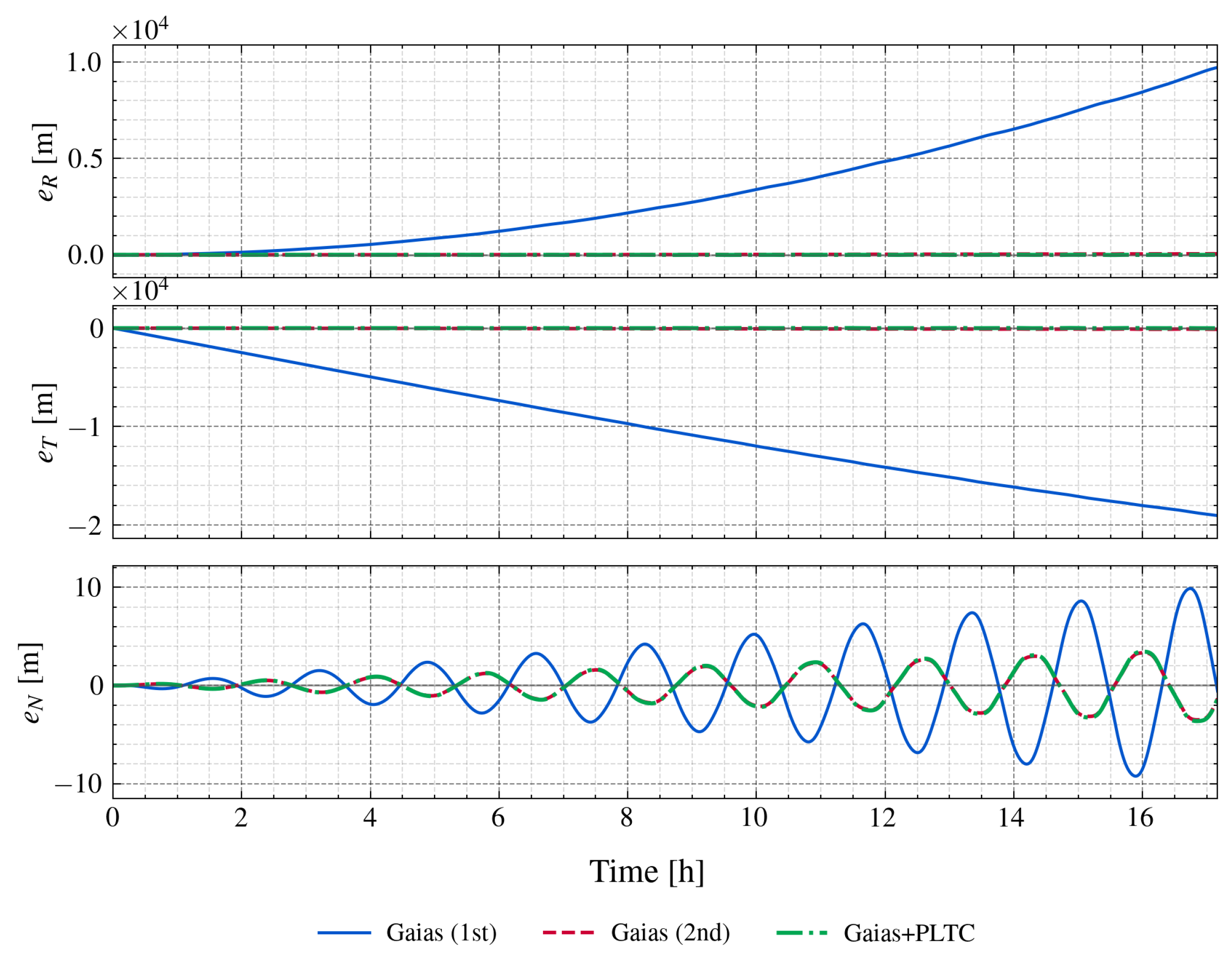
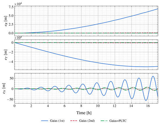
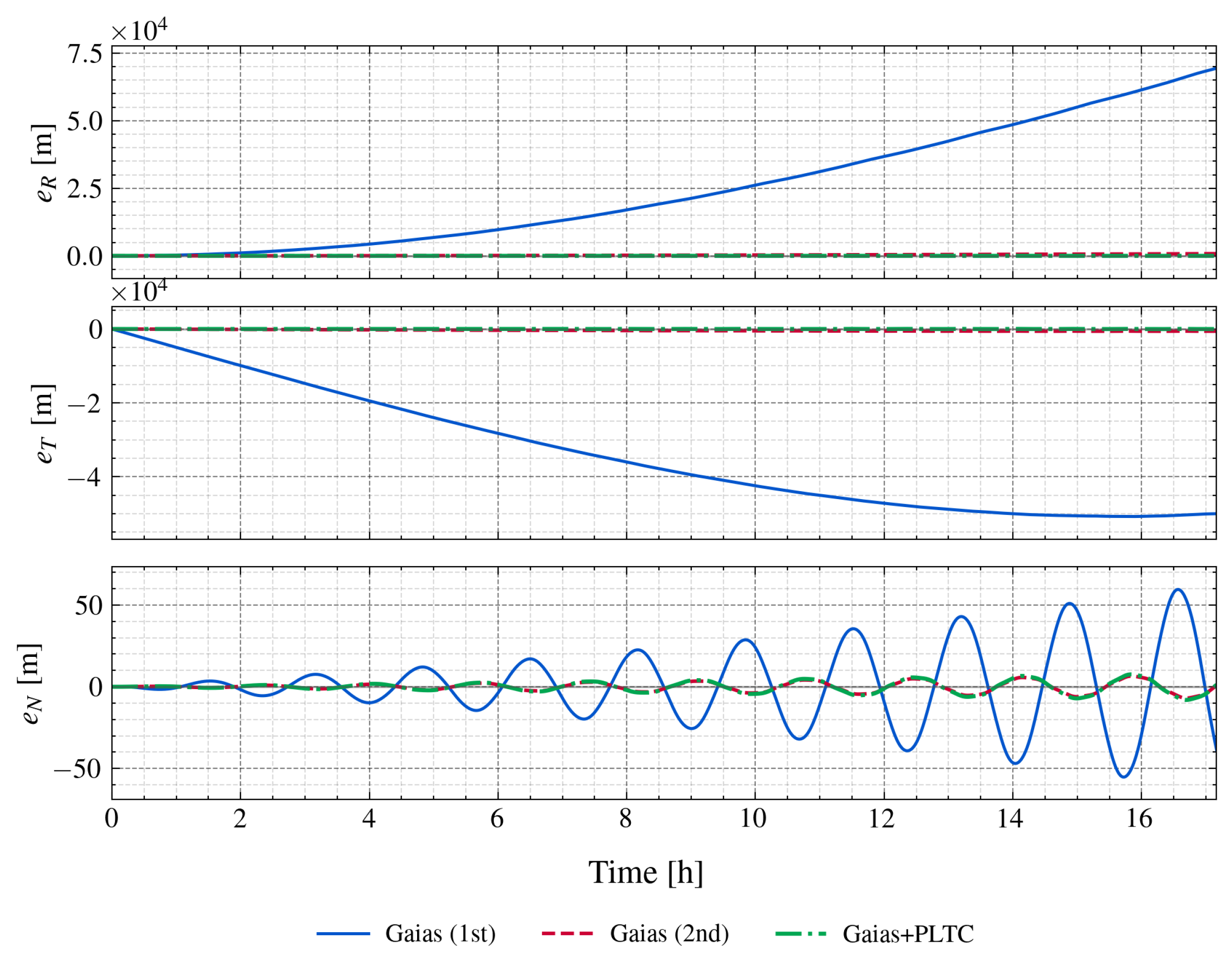
Figure 3, Figure 4 and Figure 5 present the RTN absolute error time histories for the zonal-framework methods at each , whereas Table 4 collects the terminal position error norms for all five methods, with Koenig methods evaluated against truth and Gaias methods against zonal truth.
Figure 3.
Scenario P1: ( km) propagation error RTN decomposition.
Figure 4.
Scenario P1: ( km) propagation error RTN decomposition.
Figure 5.
Scenario P1: ( km) propagation error RTN decomposition.
Table 4.
Terminal position error norm comparison (units: km; ten-revolution propagation). Koenig methods evaluated against truth; Gaias methods against zonal truth.
The error growth ratios of the first-order models (Koenig and Gaias first-order) in Table 4 closely match the prediction (ratio 4.00), confirming that first-order power-law truncation is the dominant error source in both and zonal frameworks. The near-identical terminal errors between Koenig and Gaias (first) at each (e.g., 21.389 vs. 21.378 km at ) confirm that both first-order STMs share the same truncation structure, differing only in the higher-order zonal terms that contribute negligibly to the leading error.
The Gaias second-order STT reduces the terminal error substantially (e.g., from 21.378 km to 0.128 km at ), but the residual grows rapidly with separation: from 0.128 km at to 7.977 km at , a increase consistent with the scaling of the second-order remainder. Both PLTC variants (Koenig + PLTC and Gaias + PLTC) display a distinctly different scaling behavior, with terminal errors that remain below 0.069 km across all configurations. The Gaias + PLTC method achieves the lowest errors (0.008–0.059 km), benefiting from the combination of exact power-law correction and higher-order zonal secular rates.
3.2.2. Mixed ROE Configuration (Scenario P2)
In a realistic debris-tracking mission, all ROE channels are nonzero, so the compensation must be verified under a mixed configuration. Scenario P2 uses ( km, close to the median of the cataloged debris population) with nonzero and components (Table 3). This scenario tests whether the coupling channel compensation introduces additional systematic bias and, through cross-comparison with P1, evaluates the generality of as the dominant truncation-error driver.
Figure 6 shows the results. The first-order models (Koenig: 31.2 km; Gaias (first): 31.2 km) confirm that the mixed-channel ROE components do not alter the truncation-dominated error budget. Both PLTC variants hold the error below 70 m, and Gaias + PLTC (59 m) outperforms Gaias (second) (160 m) by .
Figure 6.
Scenario P2 (mixed ROE; ) propagation error RTN component time series.
Cross-comparison with P1 confirms that is the primary error driver. For , the scaling law verified in P1 predicts a Koenig error of approximately km; the actual value is 31.2 km (deviation below 0.1%). This close agreement shows that dominates the truncation error even when and are nonzero. The Gaias + PLTC terminal error of 59 m in P2 confirms that no additional bias was introduced by the coupling channel compensation in this configuration.
3.3. Monte Carlo Filtering Validation
The propagation results establish that PLTC eliminates the leading-order truncation drift in both the and zonal frameworks. The following 500-run Monte Carlo experiments assess whether this improvement carries over to the filter solution under three observation schedules (Scenarios F1–F3). The EKF comparison focuses on the three Gaias-framework methods—Gaias (first-order), Gaias (second-order), and Gaias + PLTC—all evaluated against the matched zonal truth model. In each figure, the sample envelope (statistical spread across trials) and the posterior envelope (filter-predicted spread) are plotted together so that their agreement or divergence directly indicates filter consistency.
3.3.1. Continuous Observation (Scenario F1)
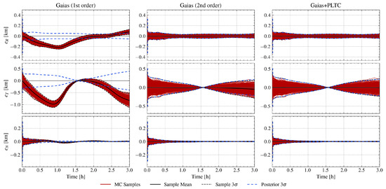
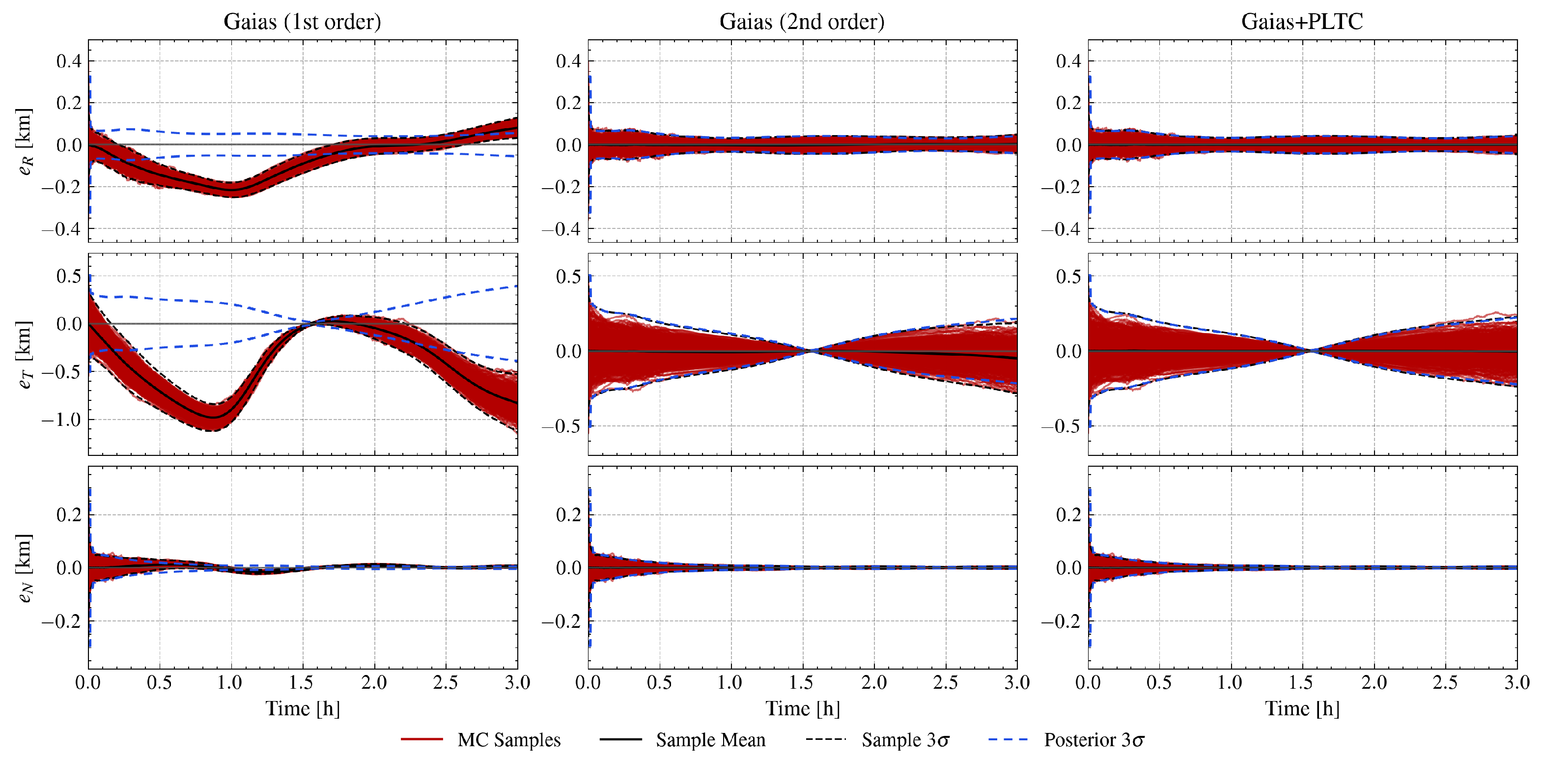
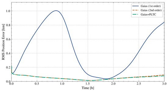
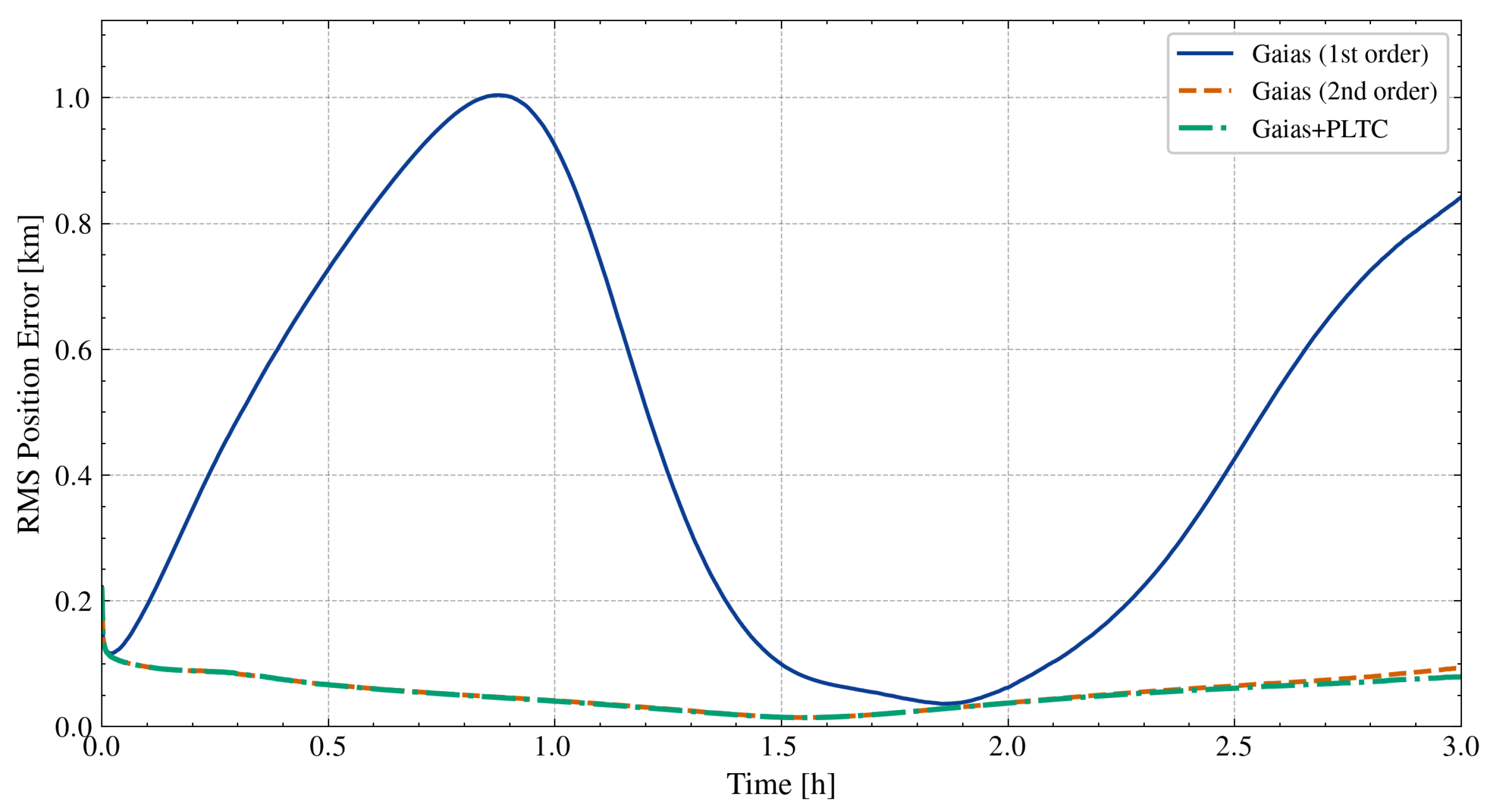
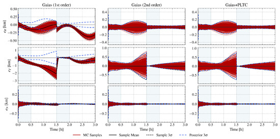
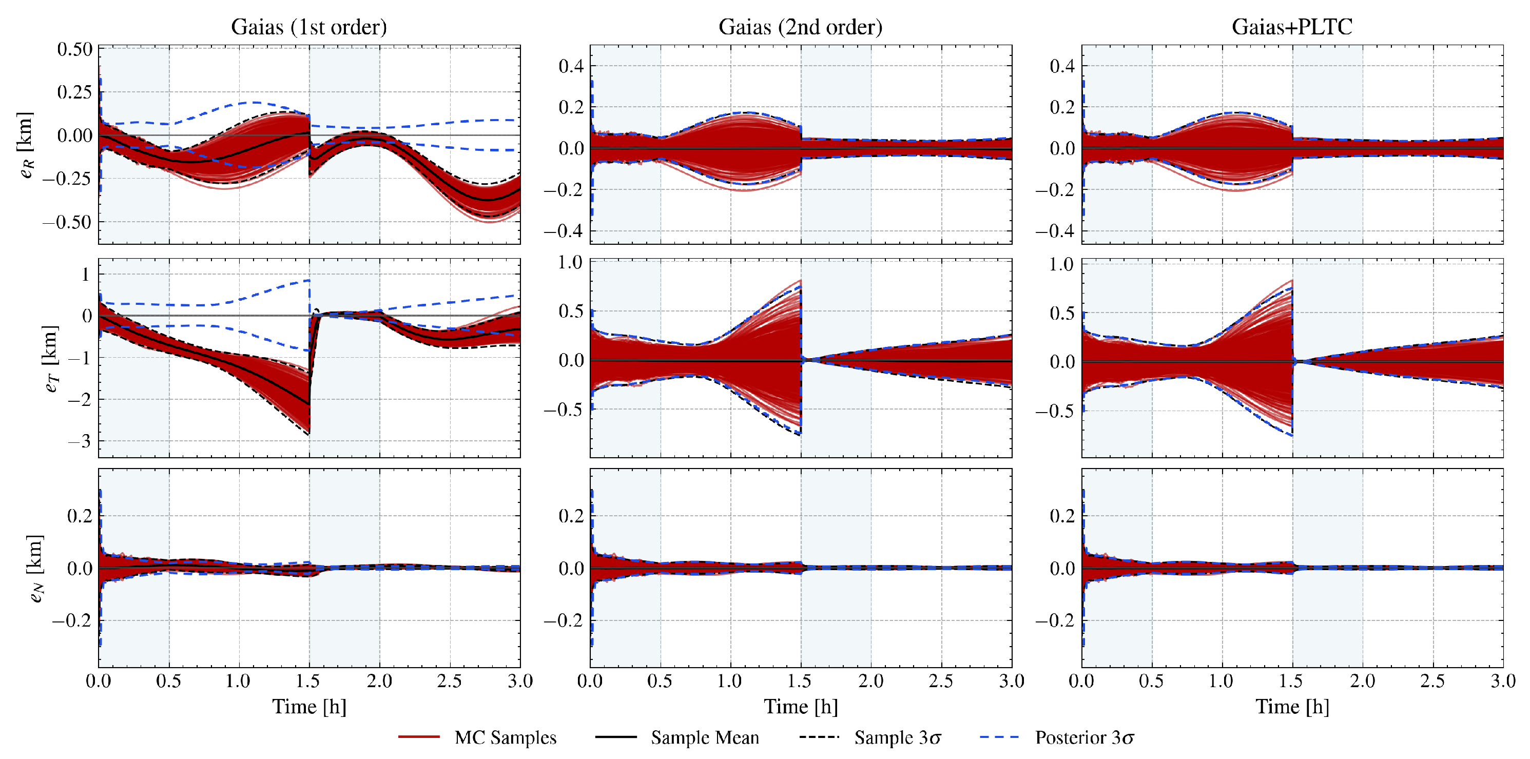
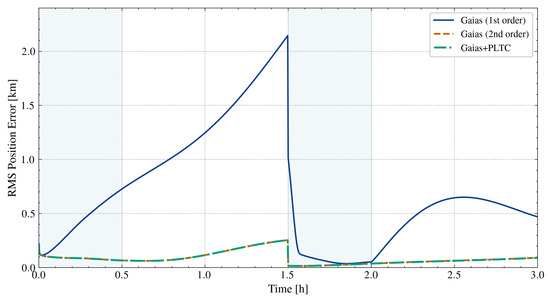
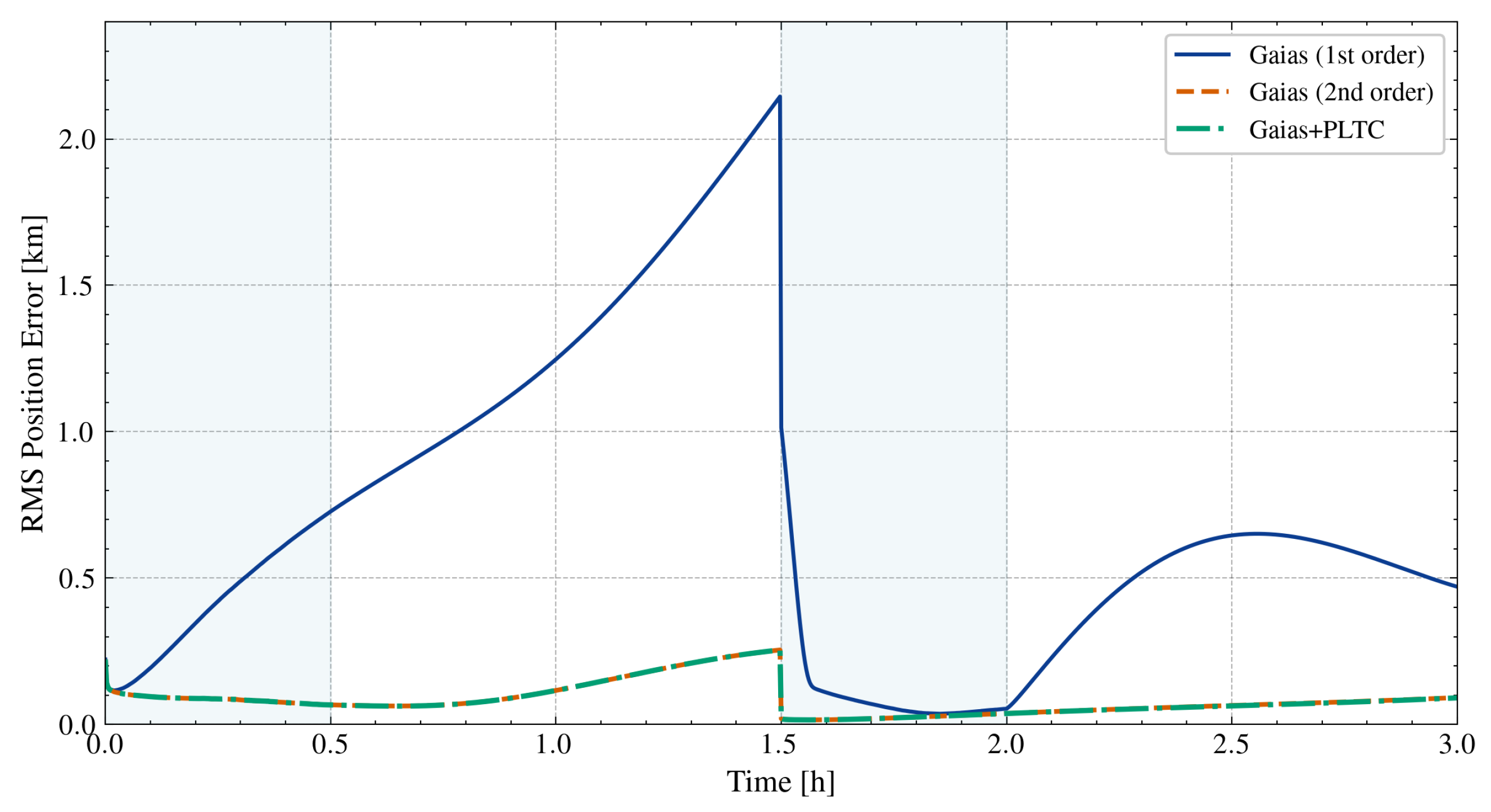
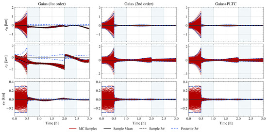
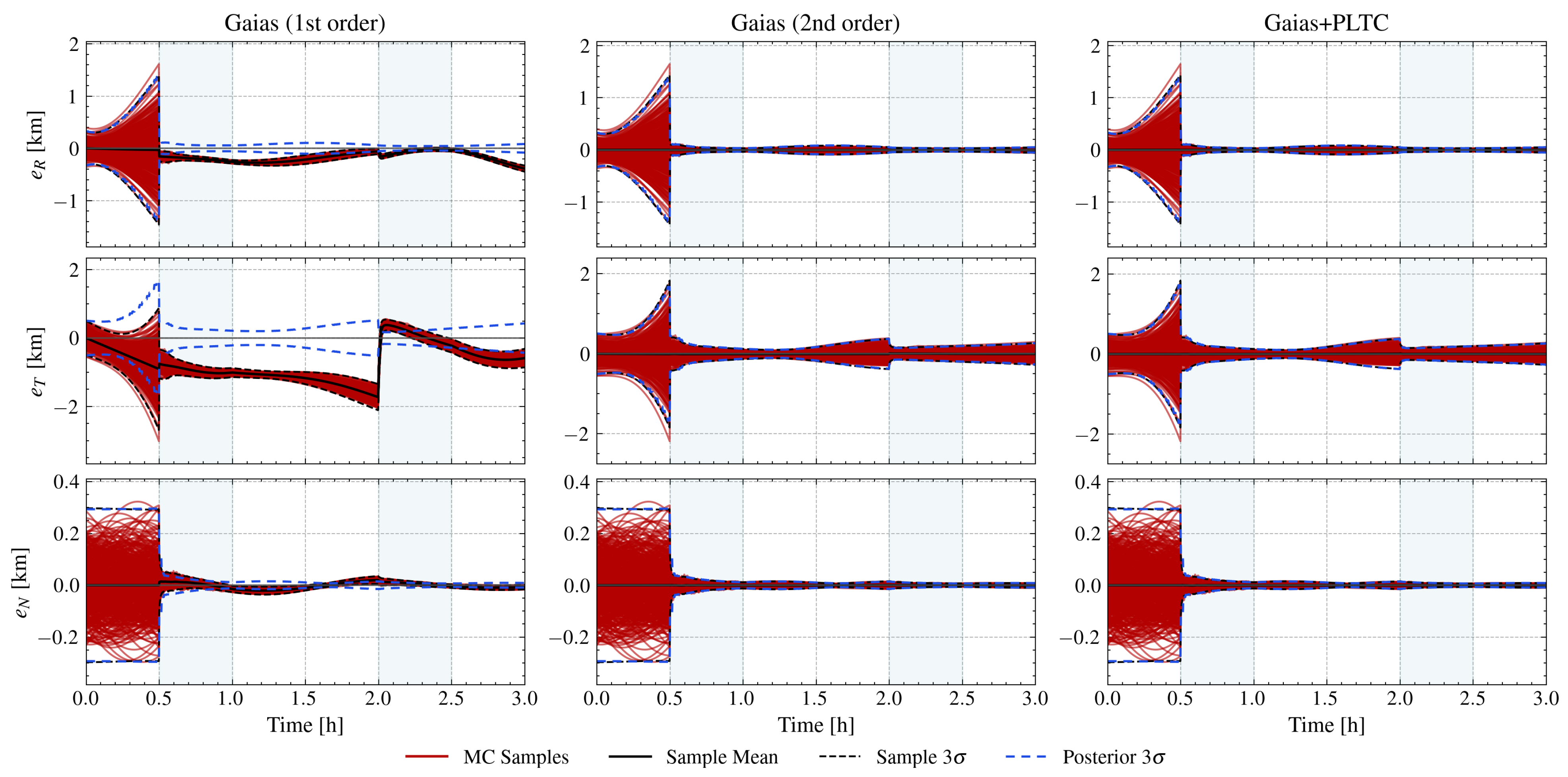
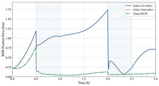
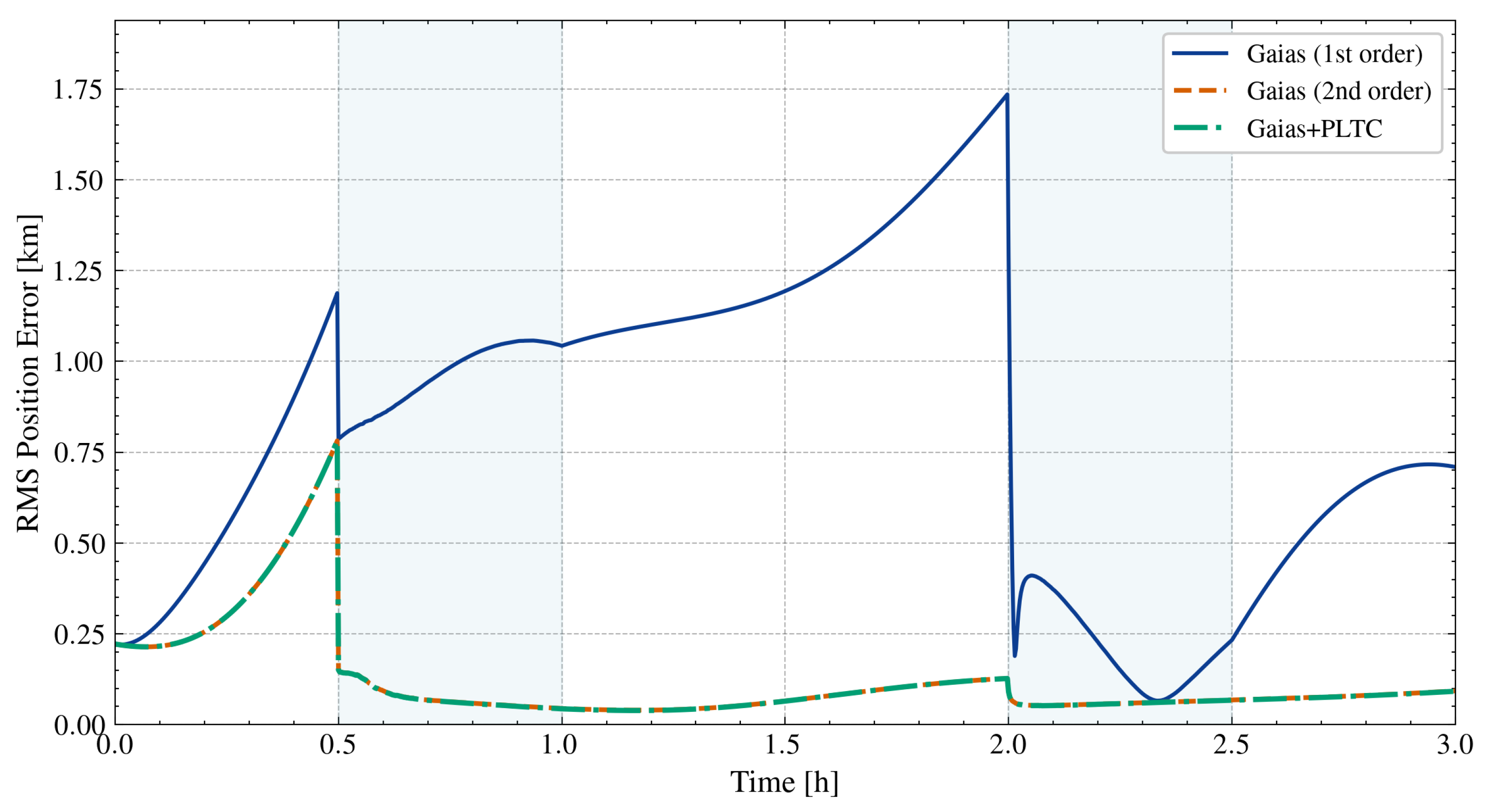
Under continuous measurements at 10 s intervals over the full 3 h window (Scenario F1), the Gaias (first-order) filter cannot fully suppress the truncation bias despite receiving the maximum possible measurement information. The terminal mean error is 836 m and the median is 839 m (hereafter P50). This reflects a structural mismatch: the inflated partially absorbs the drift, yet the deterministic component continues to accumulate between updates and eventually overwhelms the corrective capacity of the filter. The Gaias (second-order) filter substantially reduces this mismatch, achieving a terminal P50 of 63 m. Gaias + PLTC eliminates the mismatch most effectively, with a terminal P50 of 55 m. The covariance envelopes in Figure 7 and Figure 8 are consistent with this interpretation: the Gaias (first) posterior envelope falls visibly below the sample spread, while the Gaias (second) and Gaias + PLTC envelopes move much closer to the sample spread, with Gaias + PLTC showing the best agreement. The temporary collapse of the along-track (T) spread near h in Figure 7 is a phase projection effect rather than a disappearance of state uncertainty. In the near-circular ROE-to-RTN mapping, , and under continuous observations the residual errors in , , and become correlated so that this linear combination passes close to zero at that orbital phase.
Figure 7.
Scenario F1 (continuous observation) MC position error distribution (N = 500). Dotted: sample ; dashed: posterior .
Figure 8.
Scenario F1 (continuous observation) MC position RMS error evolution (N = 500).
3.3.2. Intermittent Observation (Scenarios F2 and F3)
Scenarios F2 and F3 share the same total observation time (60 min) but distribute the windows differently: F2 observes during 0–30 and 90–120 min, F3 during 30–60 and 120–150 min. This design follows the imperfect observation cases of Yang et al. [14], who tested continuous and intermittent visibility at comparable separations (25–55 km) with the same 10 s sampling; the 30-min arcs conservatively approximate the sunlit fraction available per orbit at 900 km SSO (∼68 min minus FOV and geometric exclusions).
The effect of gap placement is substantial for the uncorrected Gaias (first) filter but negligible for the corrected methods. The Gaias (first) terminal P50 differs markedly between schedules: 453 m in F2 versus 706 m in F3 (Figure 9, Figure 10, Figure 11 and Figure 12). F3 performs worse because its windows miss the initial observation period entirely, forcing the filter to coast on the biased process model from the outset. The Gaias (second) and Gaias + PLTC terminal P50 values are effectively invariant to the schedule: Gaias (second) achieves 64 m in F2 and 61 m in F3; Gaias + PLTC achieves 61 m in F2 and 60 m in F3. Once the dominant drift is removed, the remaining error is driven by observation geometry and noise, both of which average out over the same total measurement arc regardless of window placement. In both scenarios, the Gaias (first) posterior envelope underestimates the sample spread, most noticeably during the opening gap of F3, whereas the Gaias (second) and Gaias + PLTC envelopes remain much better matched, with Gaias + PLTC again giving the closest agreement.
Figure 9.
Scenario F2 (intermittent A) MC position error distribution (N = 500). Dotted: sample ; dashed: posterior .
Figure 10.
Scenario F2 (intermittent A) MC position RMS error evolution (N = 500).
Figure 11.
Scenario F3 (intermittent B) MC position error distribution (N = 500). Dotted: sample ; dashed: posterior .
Figure 12.
Scenario F3 (intermittent B) MC position RMS error evolution ().
3.3.3. Terminal Error Statistics and Cross-Scenario Summary
Table 5 shows that the Gaias (second) and Gaias + PLTC terminal P50 values remain between 55 and 64 m across all three schedules, while the Gaias (first) P50 ranges from 453 to 839 m. The Gaias (first) filter performs worst under continuous observation (F1, P50 = 839 m), where three hours of truncation bias accumulate against a continuously updated (hence small) covariance; F2 and F3 experience covariance growth during gaps that partially accommodate the drift. Both the Gaias (second) and Gaias + PLTC methods reduce the terminal error by more than an order of magnitude relative to the uncorrected first-order model, with Gaias + PLTC achieving marginally lower errors than Gaias (second) in all three schedules.
Table 5.
MC terminal position error statistics (mixed ROE config; units: m, N = 500). P90 denotes the 90th percentile.
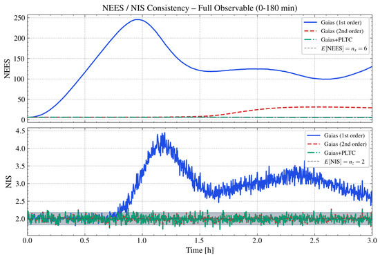
3.3.4. NEES/NIS Consistency Test
The preceding analysis quantifies position accuracy but does not directly assess statistical consistency, that is, whether the filter covariance faithfully represents the estimation error distribution. This section applies the NEES and NIS tests [34] within the MC framework.
For the i-th MC trial at epoch k, the NEES is defined as
and the NIS as
where is the innovation covariance. For a consistent filter, the N-trial average satisfies with expectation , and with expectation .
Figure 13 shows the NEES and NIS time histories for the continuous-observation baseline (F1), with 95% confidence bands shaded. The NEES of the Gaias (first) filter rises sharply, indicating that the state covariance severely underestimates the actual estimation error. The truncation drift acts as an unmodeled systematic bias that the covariance cannot represent. Gaias + PLTC, by contrast, maintains NEES close to the theoretical expectation of six throughout. The Gaias (second) model occupies an intermediate regime: its NEES is drastically lower than that of the uncorrected first-order filter, but remains above nominal because the second-order tensor removes most, but not all, of the residual process–model mismatch. On the NIS side, both Gaias (second) and Gaias + PLTC average close to the expected value of 2.0, whereas Gaias (first) shows elevated NIS values, reflecting contamination of the measurement update by the accumulated drift.
Figure 13.
Scenario F1 (continuous observation) NEES and NIS time histories (). Shaded: 95% bounds; dashed: expected values.
Table 6 summarizes the NEES/NIS statistics across all three scenarios. The Gaias (first) NEES worsens under intermittent observations because the truncation bias accumulates uncorrected during each gap and persists after observations resume—the posterior covariance, driven tight by prior updates, cannot accommodate the accumulated drift.
Table 6.
MC NEES/NIS consistency test statistics (, , and ; overline denotes the time average across the propagation arc).
Gaias + PLTC is largely unaffected by these dynamics: its time-averaged NEES remains close to the theoretical expectation of across all three scenarios, and its NIS stays close to the expected value of . Gaias (second) is still far more consistent than Gaias (first), but its time-averaged NEES remains above nominal (7.6–15.6), indicating residual model mismatch. For both corrected models, the NIS remains close to the expected value, which is operationally preferable to the Gaias (first) filter whose NEES and, under F2/F3, NIS substantially exceed the expected values.
3.3.5. Multi- Filtering Validation
The preceding experiments are restricted to a single ( km). To verify that the advantage of the corrected methods persists at larger separations, additional 500-trial Monte Carlo campaigns were conducted at (–146 km), using continuous observation (F1), the same initial covariance , and independently calibrated process noise Q for each value.
Table 7 presents the terminal median position error. Across the three pure- cases (, 73, and 146 km), the Gaias (first) and Gaias (second) errors both increase rapidly with separation, whereas the Gaias + PLTC P50 remains nearly flat at 91–93 m. The 44 km row corresponds to the mixed-ROE baseline rather than to the pure- sweep, and is included only as a reference point. Relative to Gaias (first), the improvement of Gaias + PLTC increases from at 36 km to at 73 km and at 146 km. Relative to Gaias (second), the improvement is modest at 36 km () but increases to at 73 km and at 146 km, showing that the advantage over Gaias (second) becomes more pronounced at larger separations.
Table 7.
Multi- MC terminal median position error (P50, units: m, N = 500, and F1 continuous observation).
3.3.6. Process Noise Robustness
The residual-based Q calibration folds unmodeled dynamics into the noise estimate; for the uncorrected Gaias (first) model, the deterministic truncation drift inflates by four orders of magnitude relative to the corrected models. To test whether the corrected models genuinely remove this dependence, the calibrated Q was uniformly scaled by and 200-trial Monte Carlo campaigns were run for each scaling under continuous observation (F1).
Table 8 shows that Gaias + PLTC accuracy is insensitive to Q scaling: the terminal P50 varies by only 2 m (55–57 m) as spans two orders of magnitude, and the time-averaged NEES stays between 4.9 and 6.4 (expected value: 6). The Gaias (second) model shows comparable terminal accuracy (P50: 70–73 m), but its time-averaged NEES remains above nominal (6.7–46.4), indicating residual model mismatch. The Gaias (first) terminal error varies by a factor of 12 (219–2536 m) and its NEES spans from 14 to 1809, confirming that the uncorrected filter relies on Q-inflation to partially mask the truncation bias. Reducing Q deprives the filter of this mechanism; increasing Q reduces the position error at the cost of covariance overestimation.
Table 8.
Q sensitivity: terminal P50 and time-averaged NEES under uniform Q scaling (N = 200, F1 continuous observation, and zonal truth).
3.4. Computational Efficiency and Operational Implications
Table 9 lists the per-step cost of the five analytical methods, evaluated in Python 3.11 with NumPy 1.26 on an AMD Ryzen AI 9 HX 370w; each entry is the median of 500 calls. The benchmarks show that PLTC doubles the cost of its baseline STM (Koenig + PLTC: 0.067 vs. 0.033 ms; Gaias + PLTC: 1.211 vs. 0.594 ms). The Gaias second-order tensor method costs 2.966 ms— more than Gaias + PLTC—because it must evaluate and contract a state transition tensor at each step, whereas PLTC only evaluates a six-element compensation vector and updates one column of the existing Jacobian. The entire PLTC modification lives inside the EKF prediction step; no additional state variables, covariance blocks, or tensor storage are introduced.
Table 9.
Per-step computational cost of the five analytical methods.
The reduction in terminal position error from hundreds of meters to tens of meters has direct implications for three ADR functions: (i) target reacquisition, where the order-of-magnitude reduction in along-track error is expected to narrow the sensor search corridor after measurement gaps; (ii) collision risk assessment, where a tighter and better-calibrated covariance can improve the reliability of probability-of-collision inputs; and (iii) onboard trajectory evaluation, where sub-kilometer analytical propagation accuracy over ten revolutions can reduce the reliance on numerical integration in preliminary screening of encounter geometries.
3.5. Applicability Boundaries
PLTC exactly compensates the power-law remainder but leaves the remaining first-order linearizations of the baseline STM unchanged. Because the first-order STM linearizes all ROE channels, small and are implicit prerequisites; PLTC inherits these requirements from whatever baseline it augments. The specific boundaries reported below were obtained under the simulation conditions of Section 3.1 ( km, , , 10 revolutions); they may shift at different altitudes or inclinations.
At large differential eccentricity , the first-order linearization of the STM eccentricity-coupling terms (columns 3–4) breaks down, and, because PLTC leaves these columns untouched, the resulting error grows unchecked. A sensitivity study sweeping from 0 to 0.1 (with ) across five chief eccentricities (–) shows that PLTC outperforms the Gaias second-order tensor method for and falls behind for , with the crossover largely independent of . The chief eccentricity , by contrast, enters only through the mean-to-osculating transformation [26], which expands the short-period corrections in powers of e; the baseline STM itself is closed-form in for arbitrary . A sensitivity sweep up to shows that this effect remains small, raising the terminal error from 18 m to 27 m.
The PLTC derivation evaluates all secular rates at the chief inclination; the compensation therefore assumes . As grows, the differential coupling—driven by the difference between and in the nodal and apsidal rates—accumulates over each revolution. A sensitivity sweep from to ( up to ) places the crossover with the Gaias second-order method at (); beyond , the second-order method is consistently superior. In both the eccentricity and inclination regimes where PLTC falls behind, the Gaias second-order tensor method is preferable because its full Hessian captures the cross-coupling that PLTC leaves to the baseline.
The matched truth models include only the even-zonal secular effects retained by each STM, so that the observed errors reflect truncation alone. To test robustness to force–model mismatch, an additional ten-revolution propagation experiment replaces the matched truth with a spherical harmonic gravity field (EGM96), with additional cases adding Harris–Priester differential drag (; /kg) and cannonball SRP (; /kg). Tesseral harmonics dominate the additional error, while drag and SRP each contribute at most tens of meters—as expected at 900 km. Under the full gravity + drag + SRP truth, the PLTC terminal error rises from 18 m to 226 m, yet the improvement over the uncorrected first-order model still exceeds two orders of magnitude. Over arcs substantially longer than the ten revolutions tested, these unmodeled perturbations—together with -driven drift—would require additional compensation.
4. Conclusions
This paper derives a closed-form power-law truncation correction (PLTC) for first-order ROE-STMs. The correction adds a compensation vector to the EKF prediction and updates one column of the Jacobian; the state dimension and STM structure are unchanged. It exactly compensates the truncated semi-major-axis power-law remainder, but it does not eliminate all higher-order mixed nonlinearities.
Over –146 km, the PLTC-corrected methods hold the ten-revolution propagation error to tens of meters versus tens to hundreds of kilometers for the uncorrected first-order models. In 500-run Monte Carlo filtering experiments, Gaias + PLTC reduces the median terminal error by one to nearly three orders of magnitude relative to the uncorrected model. At km, Gaias + PLTC stays below 100 m while the Gaias second-order residual reaches 1.2 km. The corrected filter maintains NEES across all observation schedules and is insensitive to Q scaling over two orders of magnitude. The PLTC overhead is the baseline STM cost and cheaper than the second-order tensor method.
The method is validated for small differential eccentricity and inclination offsets (Section 3.5), and 3 h filtering arcs at 900 km altitude. Future work will extend PLTC to eccentric orbits, develop online drag estimation, and verify timing on flight hardware.
Author Contributions
Conceptualization, S.X. and J.S.; methodology, S.X.; software, S.X.; validation, S.X.; formal analysis, S.X.; writing—original draft, S.X.; Writing—review and editing, J.S.; supervision, J.S.; and funding acquisition, J.S. All authors have read and agreed to the published version of the manuscript.
Funding
This research was funded by the the Fundamental Research Funds for the Central Universities, China (Grant No. 2042022dx0001).
Data Availability Statement
The data presented in this study are available on request from the corresponding author.
Acknowledgments
During the preparation of this manuscript, the authors used ChatGPT v5.4 for English language editing and polishing of the manuscript text. The authors have reviewed and edited the output and take full responsibility for the content of this publication.
Conflicts of Interest
The authors declare no conflicts of interest.
Abbreviations
The following abbreviations are used in this manuscript:
| ADR | Active Debris Removal |
| EKF | Extended Kalman Filter |
| LEO | Low Earth Orbit |
| NEES | Normalized Estimation Error Squared |
| NIS | Normalized Innovation Squared |
| PLTC | Power-Law Truncation Correction |
| ROE | Relative Orbital Elements |
| RTN | Radial–Transversal–Normal |
| STM | State Transition Matrix |
References
- Klinkrad, H. Space Debris: Models and Risk Analysis; Springer: Berlin/Heidelberg, Germany, 2006. [Google Scholar]
- Flegel, S.; Gelhaus, J.; Wiedemann, C.; Vörsmann, P.; Oswald, M.; Stabroth, S.; Klinkrad, H.; Krag, H. The MASTER-2009 Space Debris Environment Model. In Proceedings of the 5th European Conference on Space Debris, ESA/ESOC, Darmstadt, Germany, 30 March–2 April 2009. [Google Scholar]
- Pardini, C.; Anselmo, L. The Short-Term Effects of the Cosmos 1408 Fragmentation on Neighboring Inhabited Space Stations and Large Constellations. Acta Astronaut. 2023, 210, 465–473. [Google Scholar] [CrossRef] [Scilit]
- McKnight, D.; Witner, R.; Letizia, F.; Lemmens, S.; Anselmo, L.; Pardini, C.; Rossi, A.; Kunstadter, C.; Kawamoto, S.; Aslanov, V.; et al. Identifying the 50 Statistically-Most-Concerning Derelict Objects in LEO. Acta Astronaut. 2021, 181, 282–291. [Google Scholar] [CrossRef] [Scilit]
- Liou, J.C. An Active Debris Removal Parametric Study for LEO Environment Remediation. Adv. Space Res. 2011, 47, 1865–1876. [Google Scholar] [CrossRef] [Scilit]
- Bonnal, C.; Ruault, J.M.; Desjean, M.C. Active Debris Removal: Recent Progress and Current Trends. Acta Astronaut. 2013, 85, 51–60. [Google Scholar] [CrossRef] [Scilit]
- Ledkov, A.S.; Aslanov, V.S. Review of Contact and Contactless Active Space Debris Removal Approaches. Prog. Aerosp. Sci. 2022, 134, 100858. [Google Scholar] [CrossRef] [Scilit]
- Vasconcelos, J.; Gaggi, S.; Amaral, T.; Bakouche, C.; Cotuna, A.; Friaças, A. Close-Proximity Operations Design, Analysis, and Validation for Non-Cooperative Targets with an Application to the ClearSpace-1 Mission. Aerospace 2025, 12, 67. [Google Scholar] [CrossRef] [Scilit]
- Phipps, C.R. L’ADROIT–A Spaceborne Ultraviolet Laser System for Space Debris Clearing. Acta Astronaut. 2014, 104, 243–255. [Google Scholar] [CrossRef] [Scilit]
- Fang, Y. Low-Earth Orbit Small Space Debris Active Removal by Space-Based Pulsed Lasers. Appl. Phys. B 2024, 130, 2. [Google Scholar] [CrossRef] [Scilit]
- Kelso, T.S. CelesTrak SATCAT (Satellite Catalog). Available online: https://celestrak.org/satcat/search.php (accessed on 13 February 2026).
- Gaias, G.; Ardaens, J.S.; Montenbruck, O. Model of J2 perturbed satellite relative motion with time-varying differential drag. Celest. Mech. Dyn. Astron. 2015, 123, 411–433. [Google Scholar] [CrossRef] [Scilit]
- Koenig, A.W.; Guffanti, T.; D’Amico, S. New State Transition Matrices for Spacecraft Relative Motion in Perturbed Orbits. J. Guid. Control. Dyn. 2017, 40, 1749–1768. [Google Scholar] [CrossRef] [Scilit]
- Yang, Z.; Shang, M.; Yin, J. Analytical Second-Order Extended Kalman Filter for Satellite Relative Orbit Estimation. Aerospace 2024, 11, 887. [Google Scholar] [CrossRef] [Scilit]
- Montenbruck, O.; Kirschner, M.; D’Amico, S.; Bettadpur, S. E/I-Vector Separation for Safe Switching of the GRACE Formation. Aerosp. Sci. Technol. 2006, 10, 628–635. [Google Scholar] [CrossRef] [Scilit]
- D’Amico, S.; Montenbruck, O. Proximity Operations of Formation-Flying Spacecraft Using an Eccentricity/Inclination Vector Separation. J. Guid. Control. Dyn. 2006, 29, 554–563. [Google Scholar] [CrossRef] [Scilit]
- D’Amico, S. Autonomous Formation Flying in Low Earth Orbit. Ph.D. Thesis, Delft University of Technology (TU Delft), Delft, The Netherlands, 2010. [Google Scholar]
- Gaias, G.; Ardaens, J.S. Flight Demonstration of Autonomous Noncooperative Rendezvous in Low Earth Orbit. J. Guid. Control. Dyn. 2018, 41, 1337–1354. [Google Scholar] [CrossRef] [Scilit]
- Kruger, J.; Koenig, A.W.; D’Amico, S. Starling Formation-Flying Optical Experiment (StarFOX): System Design and Preflight Verification. J. Spacecr. Rocket. 2023, 60, 1755–1777. [Google Scholar] [CrossRef] [Scilit]
- Koenig, A.W.; D’Amico, S. Robust and Safe N-Spacecraft Swarming in Perturbed Near-Circular Orbits. J. Guid. Control. Dyn. 2018, 41, 1643–1662. [Google Scholar] [CrossRef] [Scilit]
- Gim, D.W.; Alfriend, K.T. State Transition Matrix of Relative Motion for the Perturbed Noncircular Reference Orbit. J. Guid. Control. Dyn. 2003, 26, 956–971. [Google Scholar] [CrossRef] [Scilit]
- Gim, D.W.; Alfriend, K.T. Satellite Relative Motion Using Differential Equinoctial Elements. Celest. Mech. Dyn. Astron. 2005, 92, 295–336. [Google Scholar] [CrossRef] [Scilit]
- Sullivan, J.; D’Amico, S. Nonlinear Kalman Filtering for Improved Angles-Only Navigation Using Relative Orbital Elements. J. Guid. Control. Dyn. 2017, 40, 2183–2200. [Google Scholar] [CrossRef] [Scilit]
- Sullivan, J.; Koenig, A.W.; Kruger, J.; D’Amico, S. Generalized Angles-Only Navigation Architecture for Autonomous Distributed Space Systems. J. Guid. Control. Dyn. 2021, 44, 1087–1105. [Google Scholar] [CrossRef] [Scilit]
- Kruger, J.; D’Amico, S. Observability Analysis and Optimization for Angles-Only Navigation of Distributed Space Systems. Adv. Space Res. 2024, 73, 5464–5483. [Google Scholar] [CrossRef] [Scilit]
- Gaias, G.; Colombo, C.; Lara, M. Analytical Framework for Precise Relative Motion in Low Earth Orbits. J. Guid. Control. Dyn. 2020, 43, 915–927. [Google Scholar] [CrossRef] [Scilit]
- Guffanti, T.; D’Amico, S. Linear Models for Spacecraft Relative Motion Perturbed by Solar Radiation Pressure. J. Guid. Control. Dyn. 2019, 42, 1962–1981. [Google Scholar] [CrossRef] [Scilit]
- Yang, Z.; Luo, Y.Z.; Zhang, J. Second-Order Analytical Solution of Relative Motion in J2-Perturbed Elliptic Orbits. J. Guid. Control. Dyn. 2018, 41, 2258–2270. [Google Scholar] [CrossRef] [Scilit]
- Willis, M.; Lovell, T.A.; D’Amico, S. Second Order Analytical Solution for Relative Motion on Arbitrarily Eccentric Orbits, AAS Paper 19-364. In Proceedings of the 29th AAS/AIAA Space Flight Mechanics Meeting, Ka’anapali, HI, USA, 13–17 January 2019. [Google Scholar]
- Huang, P.; Li, H.; Wen, G.; Wang, Z. Application of Adaptive Weighted Strong Tracking Unscented Kalman Filter in Non-Cooperative Maneuvering Target Tracking. Aerospace 2022, 9, 468. [Google Scholar] [CrossRef] [Scilit]
- Mu, R.; Chu, Y.; Zhang, H.; Liang, H. A Multiple-Step, Randomly Delayed, Robust Cubature Kalman Filter for Spacecraft-Relative Navigation. Aerospace 2023, 10, 289. [Google Scholar] [CrossRef] [Scilit]
- Zhou, X.; Qiao, D.; Li, X. Neural network-based method for orbit uncertainty propagation and estimation. IEEE Trans. Aerosp. Electron. Syst. 2024, 60, 1176–1193. [Google Scholar] [CrossRef] [Scilit]
- Peng, H.; Bai, X. Comparative evaluation of three machine learning algorithms on improving orbit prediction accuracy. Astrodynamics 2019, 3, 325–343. [Google Scholar] [CrossRef] [Scilit]
- Bar-Shalom, Y.; Li, X.R.; Kirubarajan, T. Estimation with Applications to Tracking and Navigation: Theory Algorithms and Software; John Wiley & Sons: Hoboken, NJ, USA, 2001. [Google Scholar]

Disclaimer/Publisher’s Note: The statements, opinions and data contained in all publications are solely those of the individual author(s) and contributor(s) and not of MDPI and/or the editor(s). MDPI and/or the editor(s) disclaim responsibility for any injury to people or property resulting from any ideas, methods, instructions or products referred to in the content. |
© 2026 by the authors. Licensee MDPI, Basel, Switzerland. This article is an open access article distributed under the terms and conditions of the Creative Commons Attribution (CC BY) license.