


Abstract
The high-speed and high-Reynolds-number conditions encountered in actual flight, coupled with the performance requirements for both low-speed climb and high-speed cruise, pose challenges for boundary-layer transition prediction and optimization in laminar design. Consequently, there are still relatively few mature and applicable high-speed laminar airfoils available. To address the insufficient validation of Reynolds-averaged Navier-Stokes (RANS) models under actual high-speed and high-Reynolds-number (Re > 107) flight conditions, the practical fidelity of the most commonly used transition model as well as NASA CFL3D solver is systematically assessed based on NASA HSNLF(1)-0213 and Honda SHM-1 high-speed business jet laminar airfoils. To the best of the authors’ knowledge, since there is no available geometry data for the SHM-1 airfoil, this is the first systematic analysis of this airfoil from a perspective other than the design team. Results demonstrate that the transition model could accurately capture natural transition and separation-induced transition at Reynolds numbers up to 16.2 × 10⁶, while also exhibiting strong robustness against variations in Mach and Reynolds number. Using the HSNLF(1)-0213 as the baseline airfoil and the design conditions of SHM-1, a multi-objective drag-reduction optimization considering climb and cruise performance was then conducted based on the Isight platform. The optimal airfoil achieves 9.53% climb drag reduction and 9.21% cruise drag reduction, revealing that aft-loading and strong favorable pressure gradients are essential to balance lift characteristics and sustain extensive laminar flow at high Reynolds numbers.
1. Introduction
Achieving high-benefit laminar design for large transport aircraft wings through aerodynamic optimization alone is challenging, owing to extremely high Reynolds number (Re) limitations. For small business jets, however, the scenario is distinct. Skin friction drag accounts for about 40% of the total drag of a small business jet, with the wing contributing approximately 61.7% [1,2]. During high-speed flights, the wing Reynolds number of business jets is typically around 2 × 10⁷ [3]. Passive laminar control could enable a large range for the laminar boundary layer, making laminar wing design highly promising for small, high-speed business jets [1,4]. When the swept angle of the wing is not significantly large for the subsonic Mach number (Ma), the laminar characteristics of the airfoil become crucial. The Dornier 228 universal transport is a typical example, in which the Do A-5 supercritical airfoil [5], as well as the trapezoidal wing with leading edge (LE) sweepback of 0° inboard and 8° outboard, is the key design element. As part of the “Wing of New Technology for General Aviation Aircraft” program, this airfoil achieved over x/c = 50% (where x means a streamwise position along the airfoil’s chord length c) laminar flow on the surface and reduced drag by up to 30% at the design point Ma = 0.37 and Reynolds number based on mean aerodynamic chord ReMAC = 7.8 × 10⁶ [5]. The HondaJet lightweight business jet features a 27° leading-edge-sweepback, and natural-laminar-flow (NLF) wing with the SHM-1 laminar airfoil [6], which is designed to extend laminar flow to x/c = 42% on the upper surface and x/c = 63% on the lower surface close to the critical Mach number. This kind of design achieved balanced low-speed climb performance (Ma = 0.31, ReMAC = 13.6 × 10⁶, lift coefficient CL = 0.35) and high-speed cruise efficiency (Ma = 0.69, ReMAC = 11.7 × 10⁶, CL = 0.26) [6]. The Phantom 3500 efficient business jet, whose maiden flight is planned in 2027, also benefits greatly from its 23° leading-edge-sweepback, super-NLF wing and an optimized airfoil [7]. Over x/c = 75% and stable laminar flow on the surface in a wide range of conditions (Ma = 0.6~0.9 and Re = 8.0 × 10⁶~15.0 × 10⁶) has been claimed by its manufacturer Otto Aerospace, which reduces the transonic drag and increases to 35% fuel efficiency, combined with a seamless, windowless composite fuselage [8]. It can be seen that laminar design is an important path to improve the flight efficiency of high-speed business jets, and laminar airfoil design is the critical stage in this process.
The foundation of laminar airfoil design is boundary-layer transition prediction, which is a classic topic. Chen et al. [9] used neural networks and random forests to map the flow parameters to transition intermittency, forming a so-called data-driven transition model. Shi et al. [10] introduced the adjoint method and analytical reverse algorithm differentiation (RAD) for derivative computation into linear stability theory (LST)-based eigenvalue problems in the eN method. Zhao [11] examined the supersonic mode evolution of boundary-layer transition under high-temperature conditions via linear parabolized stability equations (LPSE). Despite these physics-based or artificial-intelligence (AI)-based advancements in recent years, a pure RANS approach is still the dominant computational fluid dynamics (CFD) method for industrial applications. Commercial CFD software, such as ANSYS Fluent and Siemens STAR-CCM+, has adopted the transition model [12,13] in earlier versions, which offers reliable predictions for natural, bypass and separation-induced transitions.
However, the transition model was developed mainly based on correlations derived from experimental data of low-Reynolds-number boundary-layer transitions, which is also true for its applications. Catalano et al. [14] conducted numerical analysis of the incompressible flow around the SD7003 airfoil at a low Reynolds number of 6.0 × 10⁴. Both a RANS-based transition model and large eddy simulation (LES) accurately captured the separation bubble formed on the upper surface. Wang et al. [15] calibrated and validated the transition model using NLR-7301 airfoil and a high-lift trapezoidal wing at Reynolds number from 3.6 × 10⁵ to 3.34 × 10⁶. Nikolaos et al. [16] investigated the promising application potential of the NLF(1)-0416 airfoil for low-speed unmanned aerial vehicles (UAV) by transition model, indicating an extended laminar flow over x/c = 30% at Reynolds numbers from 1.0 × 10⁶ to 2.0 × 10⁶. Robitaille et al. [17] applied the transition model to design adaptive laminar airfoils in transonic conditions. They found that adaptive skin systems provided a larger range of laminar flow at medium Reynolds numbers (2.7 × 10⁶~3.1 × 10⁶), while a minimal range was possible at high Reynolds numbers, such as 12.0 × 10⁶. However, validation under Reynolds numbers exceeding 107 is insufficient, which will greatly affect the reliability of the transition model for use in practical engineering, especially in the high-speed business jet airfoil design mentioned earlier. Actually, as with the turbulence models that were rapidly developed in the 1970s and 1980s, whose high reliability has been established in engineering applications only in the past decade, the RANS transition models still require extensive validation studies focusing on actual flight conditions.
This study adopted representative high-speed laminar airfoils of business jets to further validate the fidelity of the transition model in boundary-layer transition prediction at actual flight conditions with high Reynolds numbers. The basic accuracy of the transition model, as well as the adopted numerical methods in the CFD solver, was firstly verified using a standard case from the AIAA 1st CFD Transition Modeling and Prediction Workshop (TMPW-1) [18], with optimal grid parameters established via grid convergence analysis. Then, the laminar flow behavior of two high-speed laminar flow airfoils, NASA HSNLF(1)-0213 and Honda SHM-1, at flight conditions (Re > 107), was predicted by the transition model, and compared with wind tunnel and flight test data. The effect of high Reynolds number on laminar characteristics was then discussed. Based on an assessment of these cases, a multi-objective optimization design for the high-speed business jet laminar airfoil was conducted, where the low-speed climb and high-speed cruise performances were considered simultaneously.
2. Basic Validation of the Transition Model
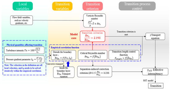
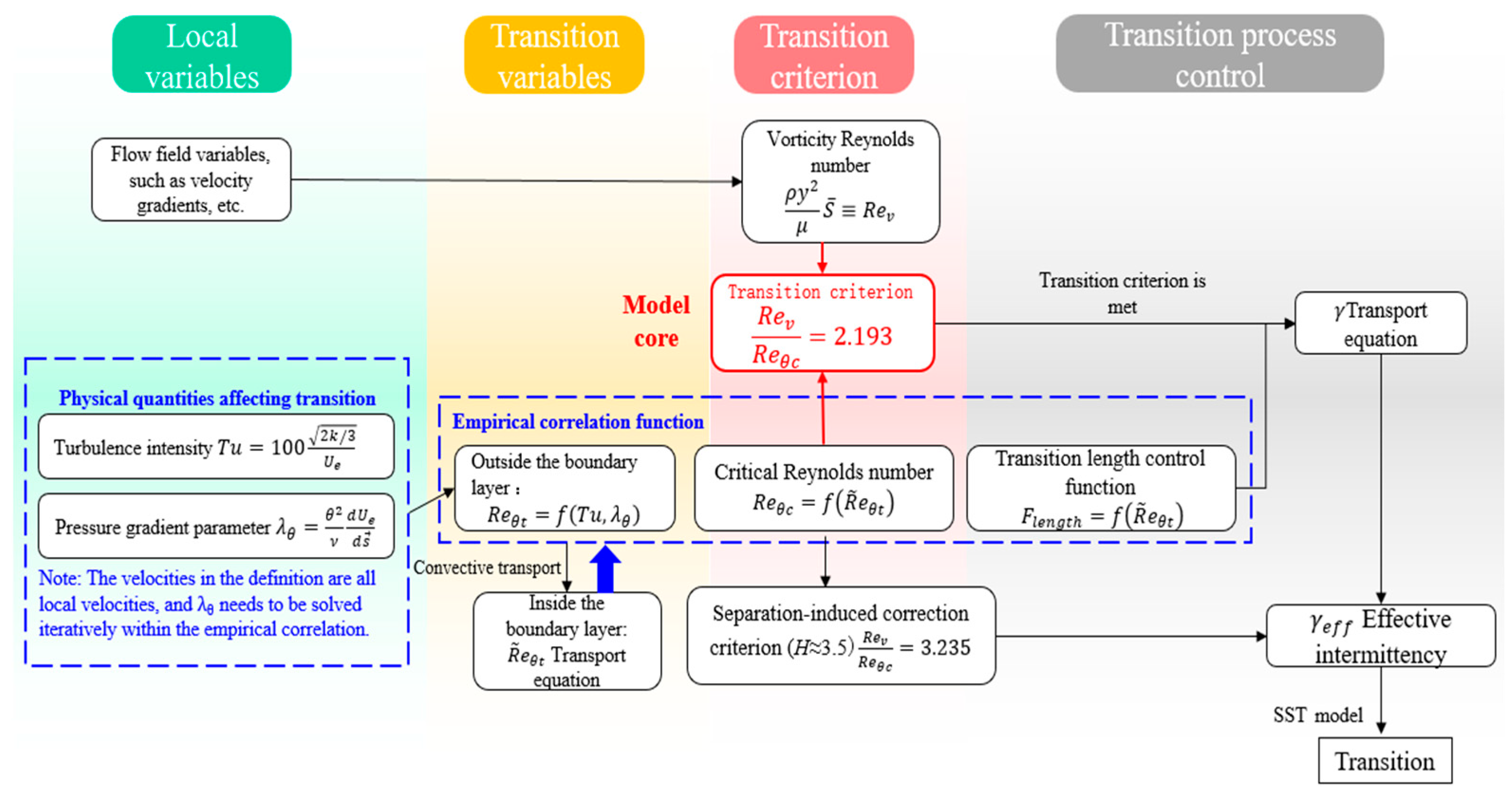
Starting in 2006, Langtry and Menter introduced the local correlation-based transition model [12,13], whose logical structure is reorganized by the authors as shown in Figure 1. The model uses transport equations to capture the transport effects of the model variables in the boundary layer during transition, especially their relationship with the external potential flow. This framework aligns with physical flow characteristics and ensures localization. The introduction of empirical correlations derived from extensive experimental data facilitates the integration of various transition mechanisms and factors into the model. As a result, the transition model has been widely applied and further developed recently [19].
Figure 1.
Logical structure of the transition model.
2.1. Numerical Methods and Case Description
All calculations in this work utilized the CFL3D solver [20] for structured grid, developed by NASA Langley Research Center (LaRC) in the early 1980s and open-sourced on GitHub in 2017. The CFL3D solves the three-dimensional, compressible, unsteady RANS equations within a finite-volume framework. The CFL3D solver supports various turbulence models, as well as the transition model based on the k-ω shear-stress-transport (SST) model. All the model equations and variables can be found on the NASA LaRC Turbulence Modeling Resource (TMR) website [19]. In this work, the convective terms of governing equations are handled with the Roe scheme and third-order MUSCL interpolation, while the viscous terms are discretized using a second-order central difference scheme. Temporal advance is achieved through an implicit approximate factorization (AF) method, which balances computational accuracy and efficiency. Message Passing Interface (MPI) parallel architecture with multigrid strategy is used to speed up the iteration. For the sake of text conciseness, the convergence history is only displayed in the first validation case below, while the remaining cases are guaranteed convergence by the authors. It should be noted that the transport equations for turbulence and transition models are solved separately from the RANS governing equations. During each iteration, the current flow field data is used to solve the turbulence and transition models, resulting in the eddy viscosity coefficient. This coefficient is then input into the RANS equations to determine the flow field for the next step. Because the flow is steady, the iterative process will converge to a solution. Furthermore, before the flow reaches the airfoil, the initial freestream turbulence intensity will decay due to transport, making the turbulence level at the LE differ from experimental conditions. Therefore, a so-called ambient source term [21] was introduced into the production term of turbulent kinetic energy to suppress the decay of freestream turbulence intensity in all the cases.
Standard case of NASA NLF(1)-0416 airfoil from (TMPW-1) was firstly used to verify the numerical methods in the NASA CFL3D solver, establishing optimal grid parameters via convergence analysis. Wind tunnel testing of the NASA NLF(1)-0416 general aviation airfoil (relative thickness 16%) was performed in the NASA Langley Low-Turbulence Pressure Tunnel (LTPT) [22]. The Reynolds number during testing ranged from 1.0 × 10⁶ to 9.0 × 10⁶, with Mach numbers from 0.1 to 0.4. The case at the conditions of Ma = 0.1 and Re = 4.0 × 10⁶ has extensive experimental data, which was also used in the AIAA 1st CFD Transition Modeling and Prediction Workshop (TMPW-1). The freestream turbulence intensity was set to 0.15% as suggested from AIAA TMPW-1 [23], while the viscosity ratio RT,inf was 12 from the authors’ experience. Owing to high background noise levels at high Reynolds numbers, the experiment only recorded TOLs at Re ≤ 4.0 × 10⁶ and small angles of attack [22].
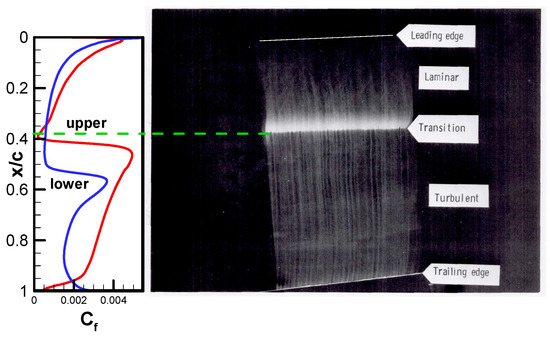
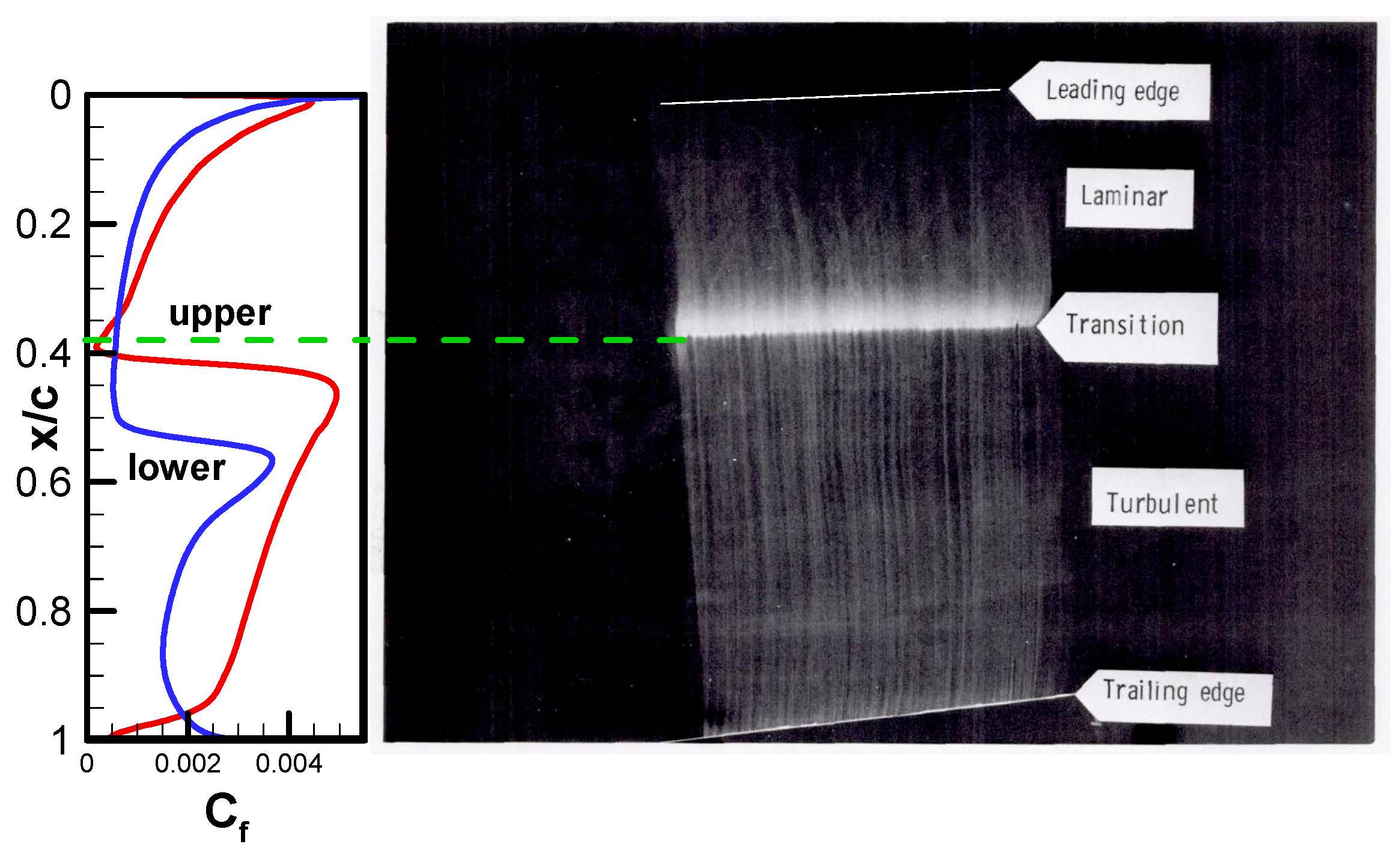
Based on the experiment, the TOL on the upper surface is roughly between x/c = 25% and 40%, while the FPG on the lower surface is quite extensive. The airfoil’s relatively large leading-edge radius makes the pressure gradient less affected by changes in the angle of attack. As the angle of attack increases, the TOL on the upper surface shifts forward slowly, and the separation bubble on the upper surface vanishes at Re = 4.0 × 10⁶. Figure 2 includes an oil-flow visualization photograph of the upper surface at Ma = 0.29, Re = 4.0 × 10⁶ and α = 0°, indicating that the transition occurs at around x/c = 35% to 40% without a separation bubble forming. The predicted result (curves on the left of Figure 2, by fine mesh in Table 1) accurately reflects this behavior.
Figure 2.
Comparison of oil-flow visualization [22] on the upper surface and predicted skin friction coefficient at Ma = 0.29, Re = 4.0 × 10⁶ and α = 0° (from the fine mesh).
Table 1.
Mesh sequence parameters of the NLF(1)-0416 airfoil for grid convergence analysis.
2.2. Grid Convergence Analysis
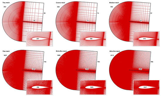
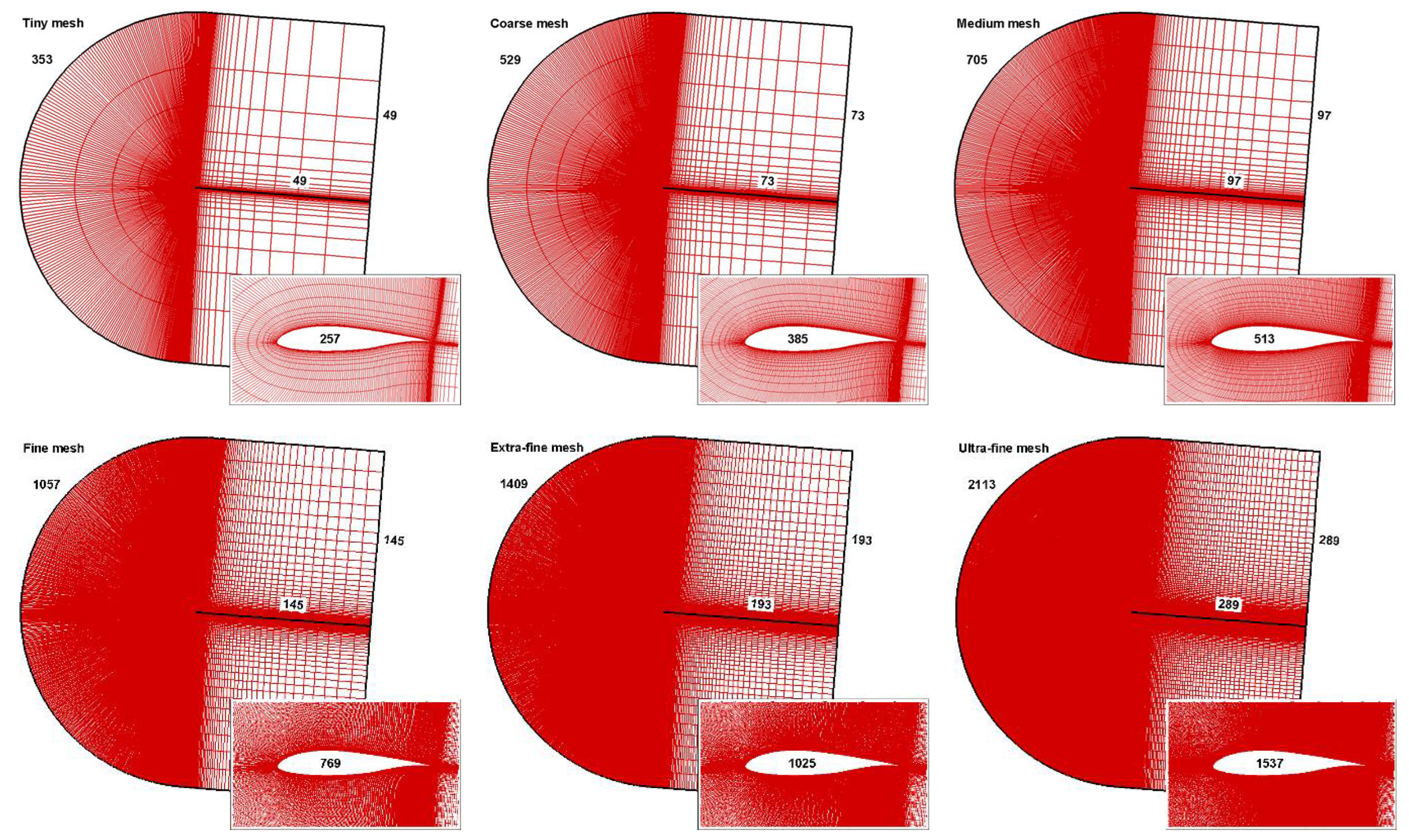
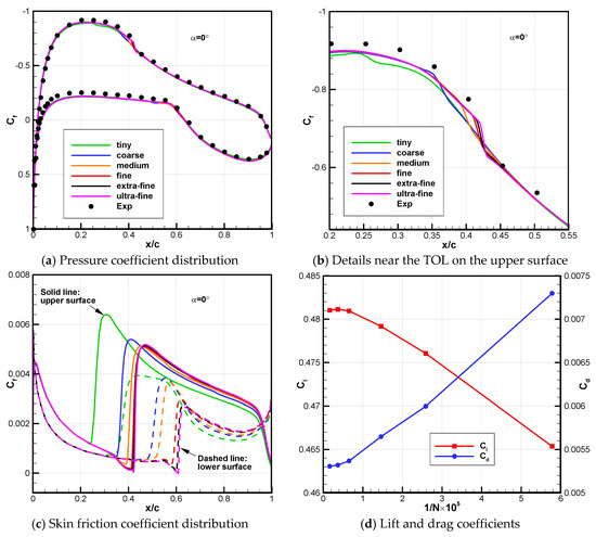
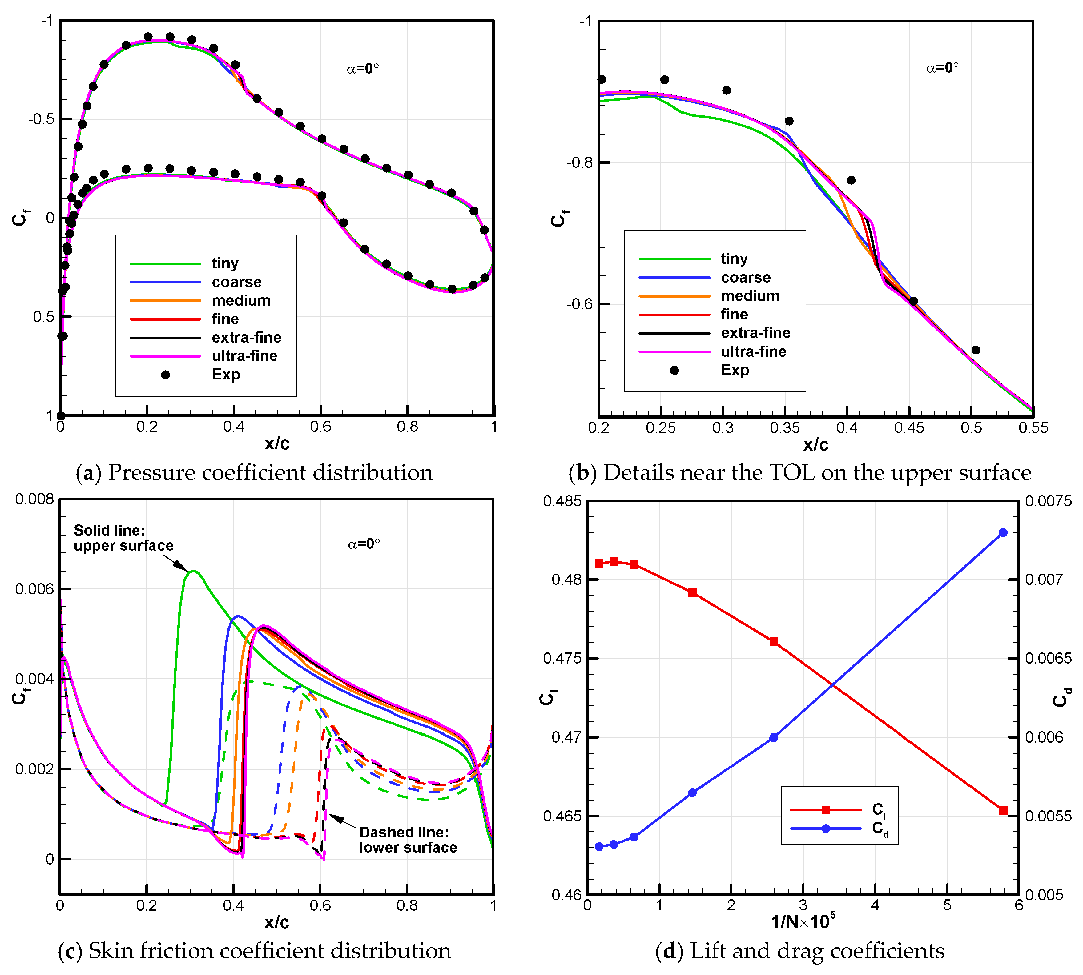
Grid convergence analysis was conducted using the standard mesh sequence (Figure 3) provided by the AIAA TMPW-1 [18]. The computational domain was rotated based on the bisector direction of the airfoil’s trailing edge angle. The parameters of different mesh in Table 1 are similar to the self-developed S809 mesh sequence. However, for high Reynolds numbers, smaller grid scales normal to the wall are required to ensure enough grid points within the thinner boundary layer. Figure 4 shows the grid convergence results for Ma = 0.1, Re = 4.0 × 10⁶ and α = 0°, where differences in pressure coefficient distribution are minor (Figure 4a) and mainly near the TOL on the upper surface (Figure 4b). More significant variation appears in TOL predictions (Figure 4c), which shift downstream as the mesh is refined and tend to converge starting from the fine mesh. This pattern is also reflected in the convergence of lift and drag coefficients (Figure 4d).
Figure 3.
Mesh sequence of the NLF(1)-0416 airfoil for grid convergence analysis.
Figure 4.
Grid convergence results for the NLF(1)-0416 airfoil at Ma = 0.1, Re = 4.0 × 10⁶ and α = 0°.
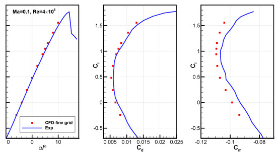
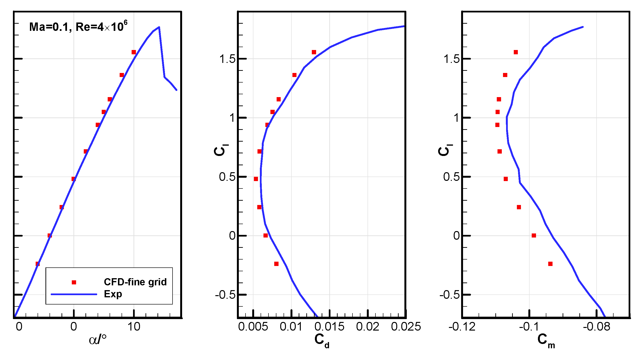
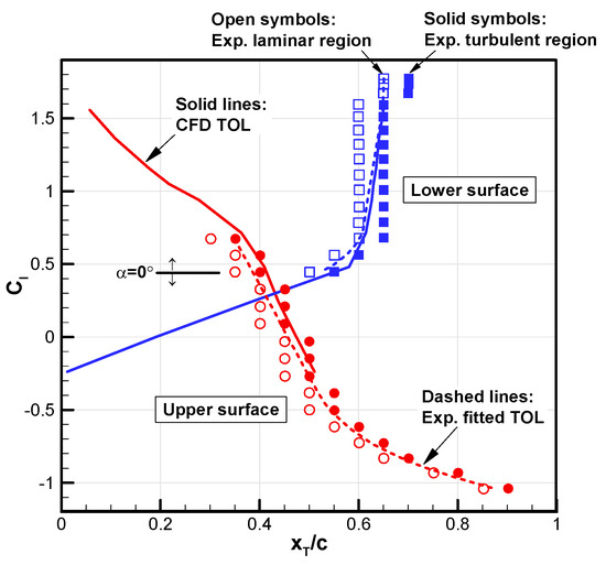
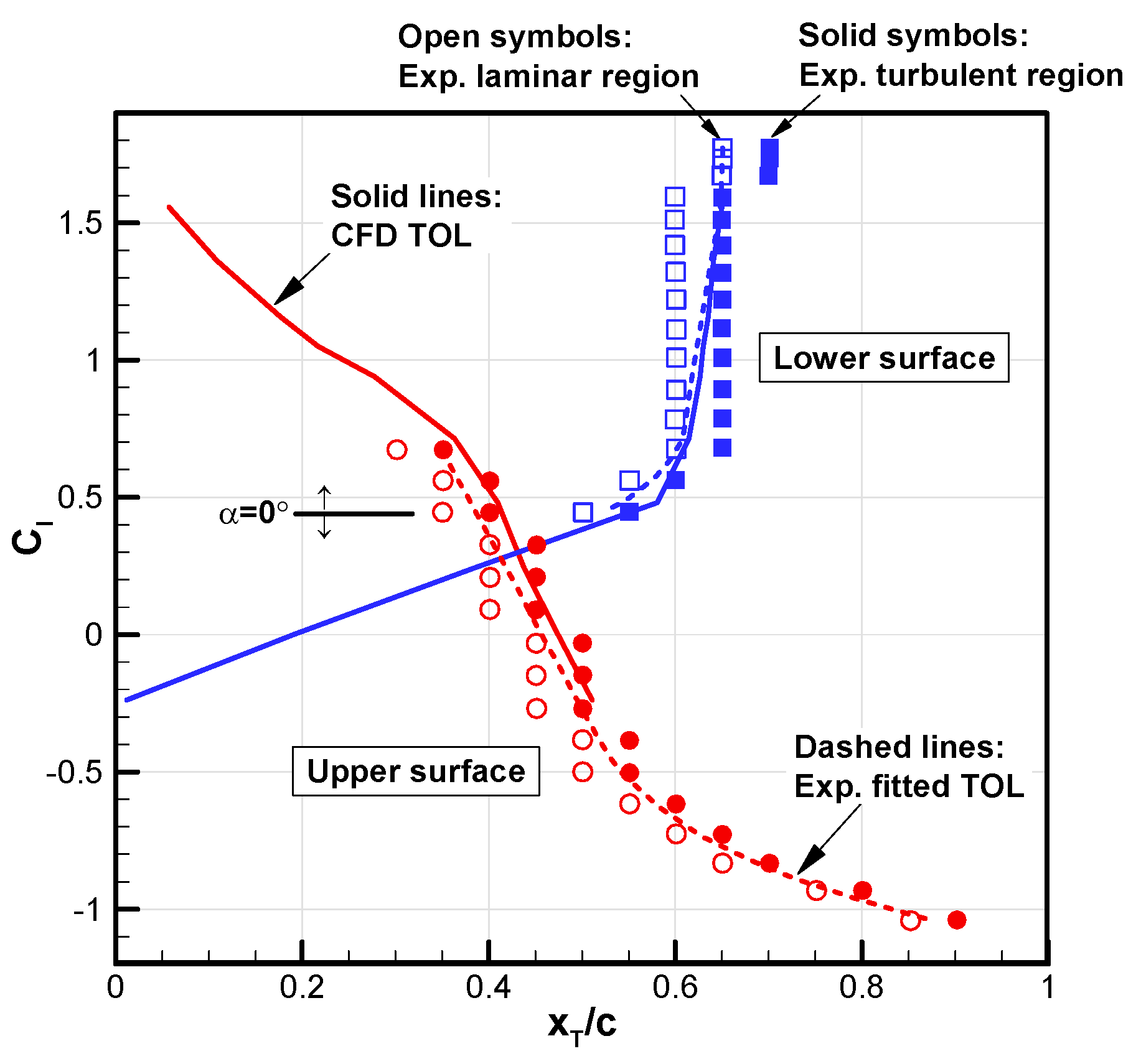
Figure 5 shows the predicted aerodynamic coefficients at Ma = 0.1 and Re = 4.0 × 10⁶ using the fine mesh. The lift and drag coefficients closely match the experimental data, while the moment coefficient shows some differences. Additionally, Figure 6 shows a comparison between the predicted and experimental TOLs for the NLF(1)-0416 airfoil at different lift coefficients (corresponding to different angles of attack). Here, the open and solid symbols represent the experimentally measured start (laminar region) and end (turbulent region) of the transition zone, respectively, together defining the zone of TOL. The dashed line is the fitted TOL curve provided in the experimental reference [22]. It can be observed that the predicted TOLs generally fall within the experimental zone and are in close agreement with the fitted curve. This validates the fundamental predictive capability of the transition model using the fine mesh.
Figure 5.
Comparisons of predicted aerodynamic coefficients with experimental data for the NLF(1)-0416 airfoil at Ma = 0.1 and Re = 4.0 × 10⁶.
Figure 6.
Comparison of predicted transition onset locations with experimental data for the NLF(1)-0416 airfoil at Ma = 0.1 and Re = 4.0 × 10⁶.
2.3. Validation at Higher Reynolds Number
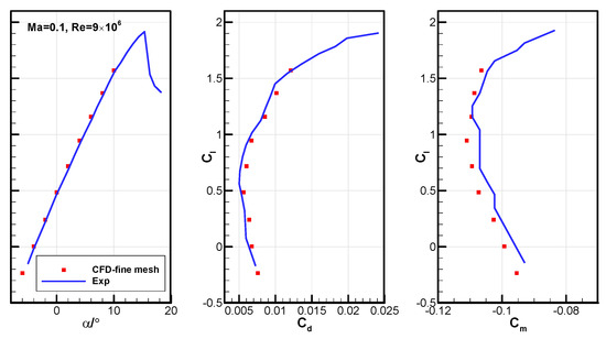
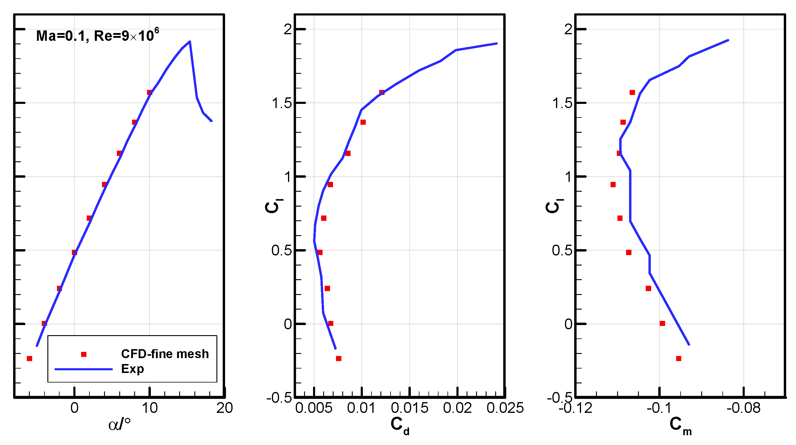
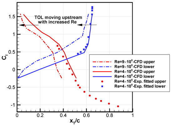
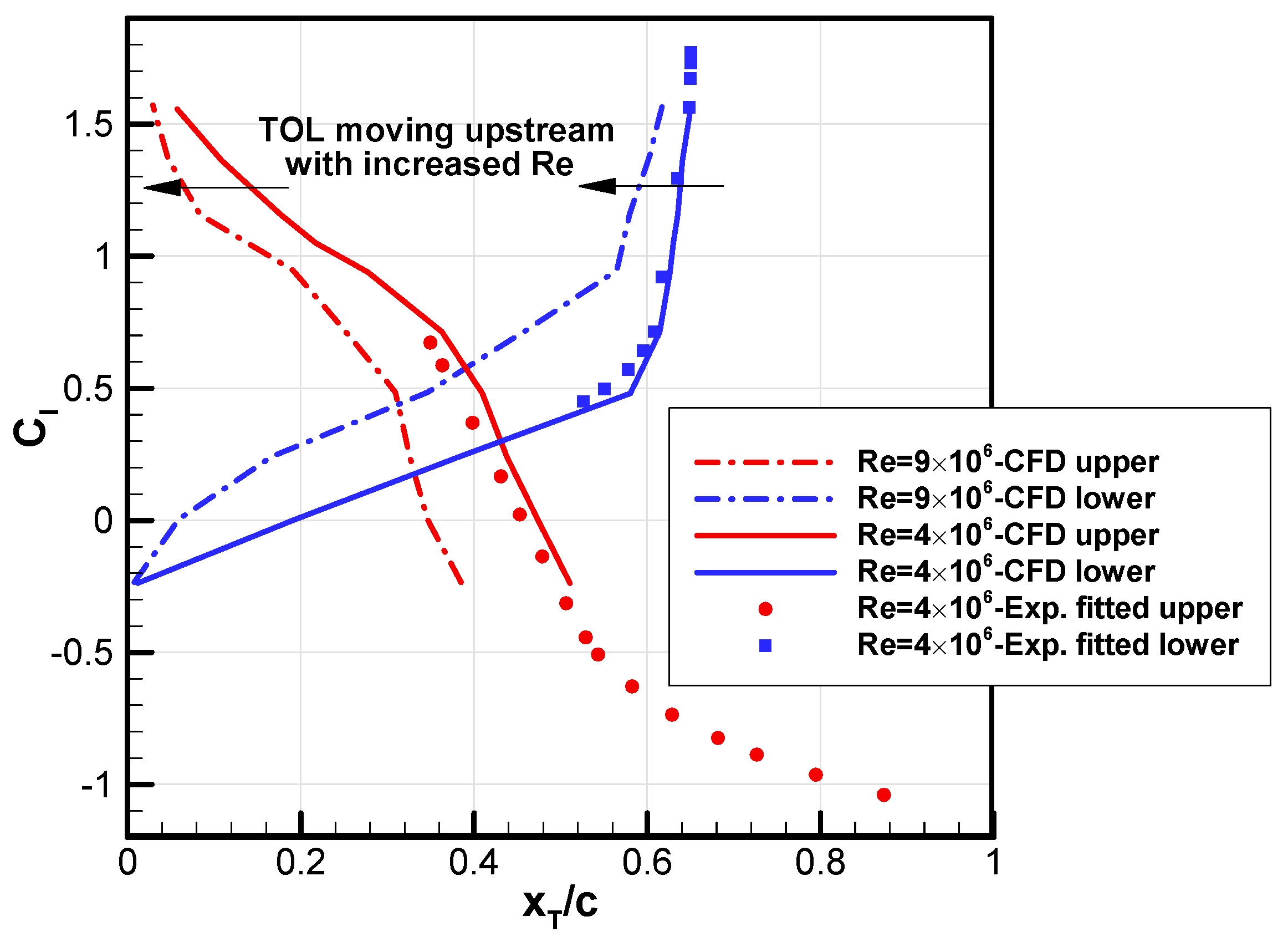
When the Reynolds number increased to 9.0 × 10⁶, the aerodynamic coefficients still closely matched the experimental data (Figure 7), while the TOLs on both the upper and lower surfaces shifted upstream at the higher Reynolds number as expected (Figure 8). Based on the results from the above cases, it is reasonable to conclude that the fine mesh level is suitable for boundary-layer transition predictions using the transition model at medium (about 5.0 × 10⁶) and larger (about 10 × 106) Reynolds numbers.
Figure 7.
Comparisons of predicted aerodynamic coefficients with experimental data for the NLF(1)-0416 airfoil at Ma = 0.1 and Re = 9.0 × 10⁶.
Figure 8.
Comparisons of predicted transition onset locations for the NLF(1)-0416 airfoil at Re = 4.0 × 10⁶ and Re = 9.0 × 10⁶.
3. Fidelity Assessment at High-Reynolds-Number Flight Conditions
Modern business jets typically operate under high-speed and high-Reynolds number conditions. The ability to predict transitions accurately in these flows is crucial for applying transition models to laminar design.
3.1. NASA HSNLF(1)-0213 High-Speed Laminar Airfoil
The successful development of the NLF-series airfoils motivated NASA to pursue high-speed NLF. Starting in 1984, some LaRC departments collaborated on designing the HSNLF (High-Speed Natural-Laminar-Flow) (1)-0213 airfoil, including a subsequent three-dimensional design for an unswept wing of a single-engine, high-speed business jet [24,25]. The design point is Ma = 0.7, Re = 11.0 × 10⁶, Cl = 0.25–0.26 (around α = −0.953°). The HSNLF(1)-0213 airfoil features a high drag-divergence Mach number and a low nose-down pitching moment. However, its 13%c thickness limits wing volume, which could impact the flight range in practical use [26].
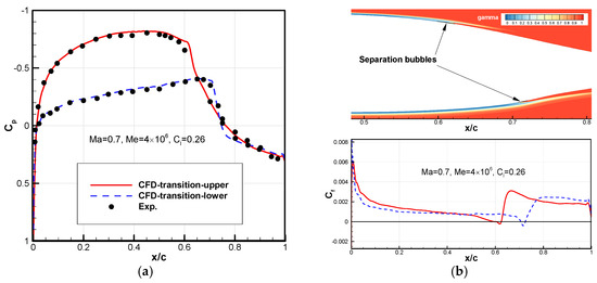
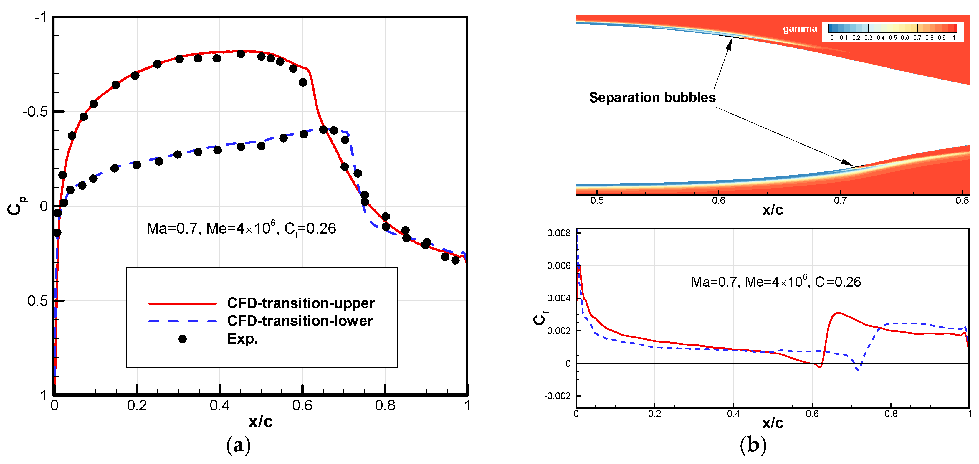
The grid parameters were the same as the fine mesh listed in Table 1 and Table 2, except that the height of the first grid layer normal to the wall was set to 1.5 × 10⁻⁶c to keep the dimensionless wall-normal grid spacing y+ below 1 across the entire surface considering higher Reynolds number. Since the experiment in the NASA Langley 6 × 28-inch Pressurized Transonic Tunnel did not provide the turbulence level conditions, a freestream turbulence intensity of 0.03% was assumed and verified by a prediction at Ma = 0.7, Re = 4.0 × 10⁶ and Cl = 0.26, with the viscosity ratio RT,inf = 5.0. Figure 9 shows the pressure and skin-friction coefficient distributions with the contour of intermittency γ. Transition induced by small separation bubbles is observed on both the upper and lower surfaces, occurring at the designed minimum pressure point. The predicted drag coefficient 0.0043 closely matches the design value 0.0041 [24].
Table 2.
Validation conditions of the SHM-1 airfoil with corresponding comparable experimental data.
Figure 9.
Predicted results of the HSNLF(1)-0213 airfoil at Ma = 0.7, Re = 4.0 × 10⁶ and Cl = 0.26. (a) Comparison of pressure coefficient distribution with experimental data; (b) intermittency γ near the airfoil with skin friction coefficient distribution.
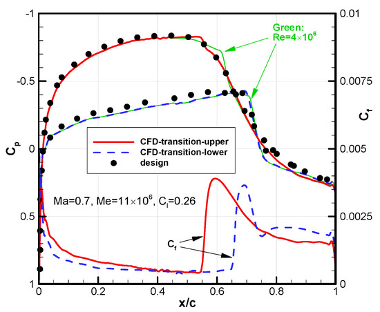
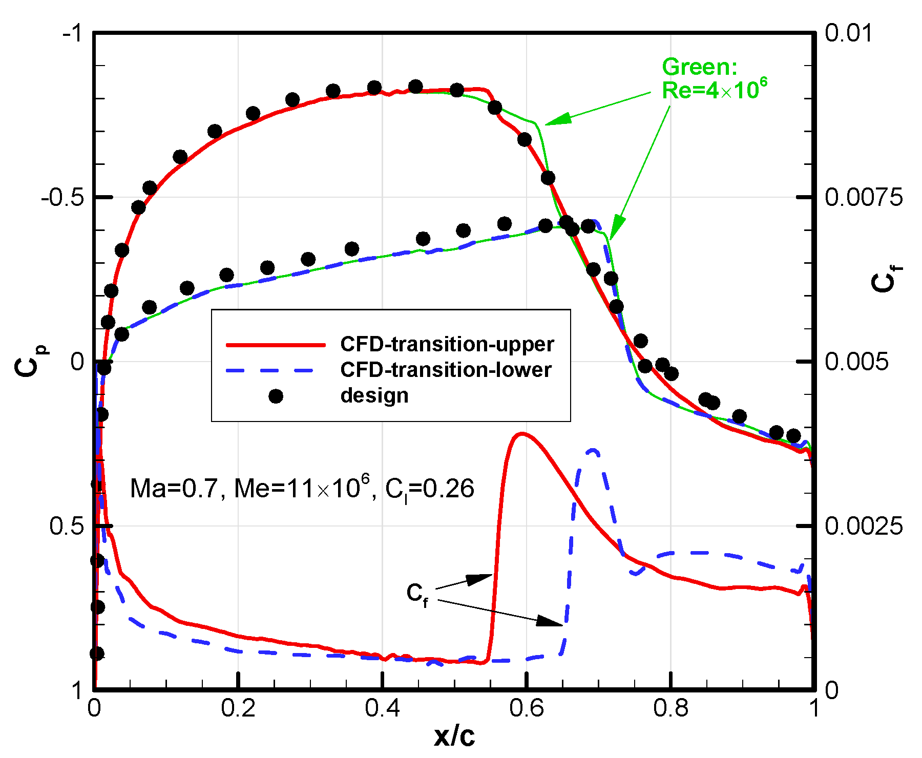
With a higher Reynolds number, Re = 11.0 × 10⁶, it is evident that the pressure distribution aligns well with the experimental data (Figure 10). Compared to the case of Re = 4.0 × 10⁶, the TOLs (shown in the skin friction coefficient distribution) have moved approximately 10%c upstream on both surfaces due to a natural transition near the minimum pressure points.
Figure 10.
Pressure and skin friction coefficient distributions on the HSNLF(1)-0213 airfoil at Ma = 0.7, Re = 11.0 × 10⁶ and Cl = 0.26.
3.2. Honda SHM-1 Natural Laminar Airfoil
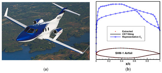
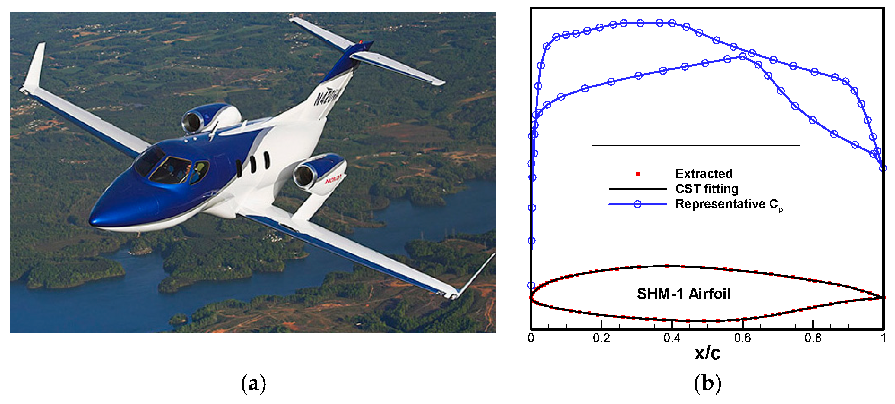
In the early 21st century, the Honda Research and Development (R&D) department launched the development of an advanced light business jet, called the HondaJet [6] (Figure 11a). It featured integrally machined skin to achieve NLF for both the wing and the fuselage nose. The airfoil was designed to balance low-speed climb performance (Ma = 0.31, Re = 13.6 × 10⁶, Cl = 0.35) with high-speed cruise efficiency (Ma = 0.69, Re = 11.7 × 10⁶, Cl = 0.26). The target for the drag-divergence Mach number was set above 0.7, and the relative thickness was 15%c to provide sufficient fuel volume. This NLF airfoil, designated as SHM-1 [26], featured laminar flow extending to x/c = 42% on the upper surface and x/c = 63% on the lower surface (both near the minimum pressure points, Figure 11b) close to the critical Mach number. This study extracted the geometry points from Ref. [26], and applied the class/shape function transformation (CST) method to fit and reconstruct the SHM-1 airfoil (Figure 11b).
Figure 11.
The HondaJet high-speed light business jet and SHM-1 airfoil. (a) The HondaJet [6]; (b) the SHM-1 airfoil with a typical pattern of pressure distribution.
Honda conducted transonic tests in the ONERA 0.56 m × 0.78 m wind tunnel and, due to the small aircraft size, performed low-speed tests on a full-scale wing in the Honda 5 m × 3.5 m wind tunnel. At the same time, flight tests were carried out by modifying a T-33 aircraft wing under actual flight conditions. The TOLs on the wing surface were recorded with an infrared camera inside the cockpit, and static pressure orifices measured the pressure coefficient. As a result, the experimental data for the SHM-1 airfoil is relatively abundant [6,26]. This paper validates transonic flight conditions (Table 2) and compares results with data from flight test and other solvers based on stability theory [6]. Since the Reynolds number during flight reached over 16 × 106, the height of the first grid layer normal to the wall was further reduced to 0.9 × 10⁻⁶c based on the earlier fine mesh distribution. The freestream turbulence intensity was set to 0.03% due to the high-altitude flight environment, with the viscosity ratio RT,inf = 10.
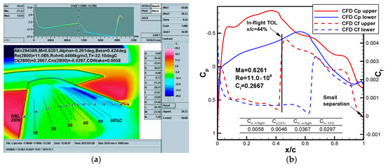
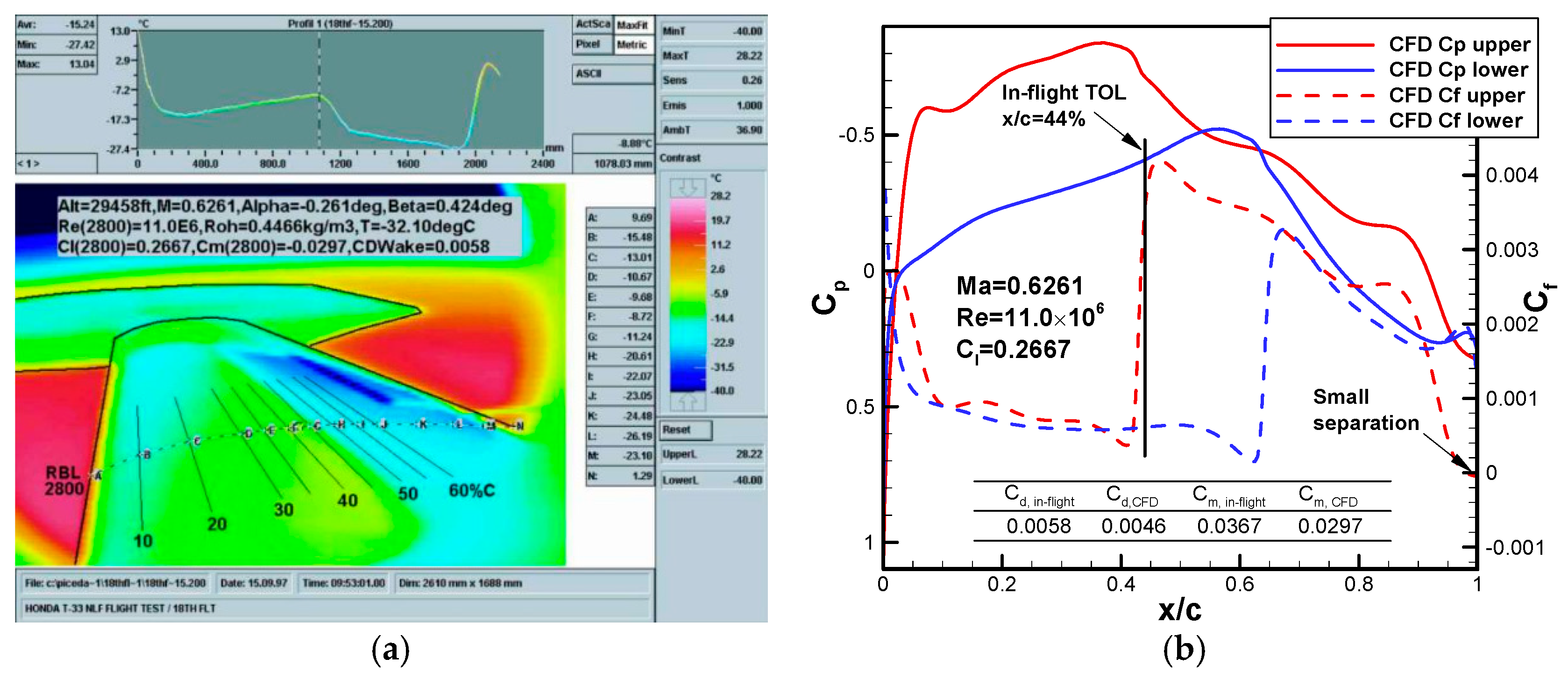
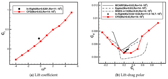
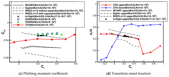
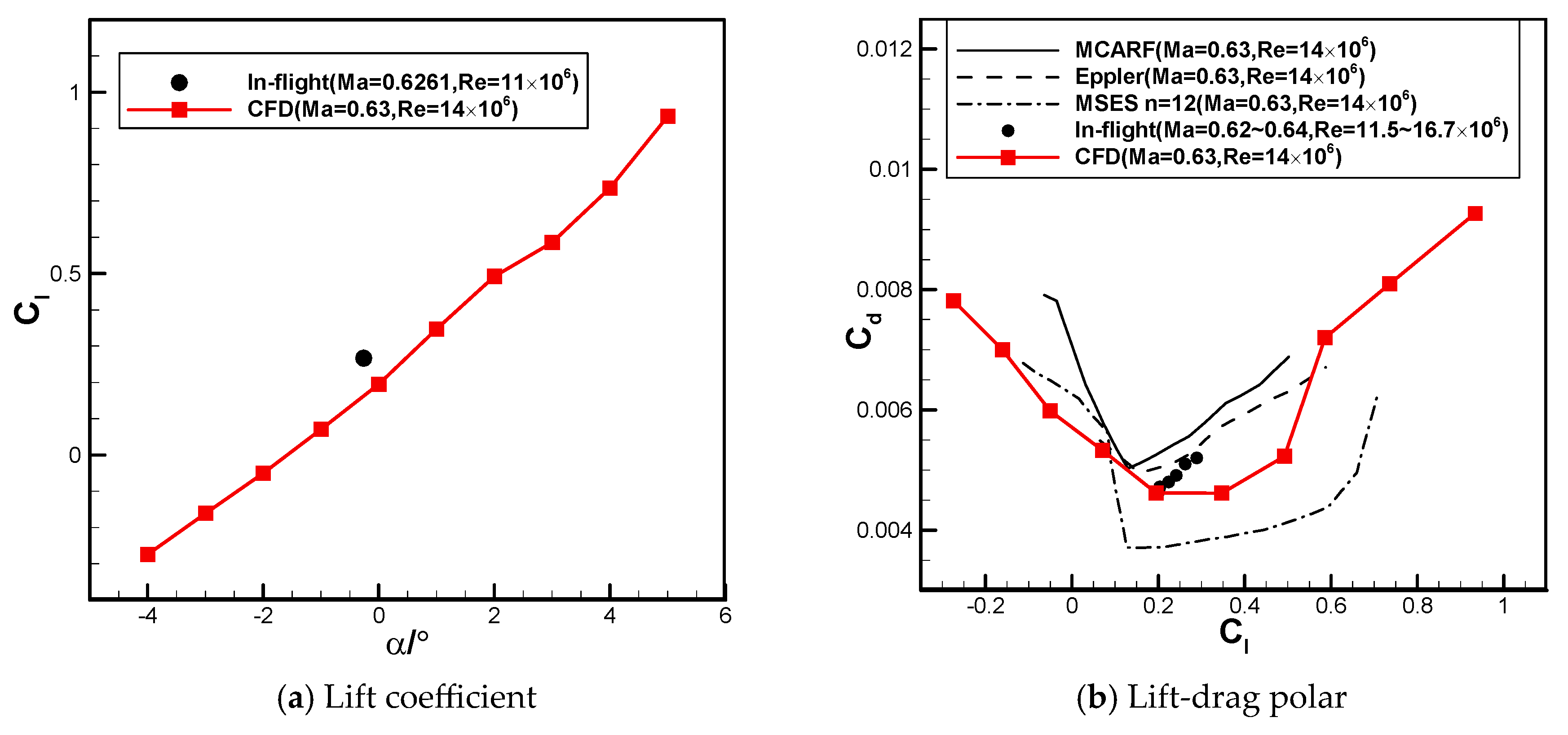
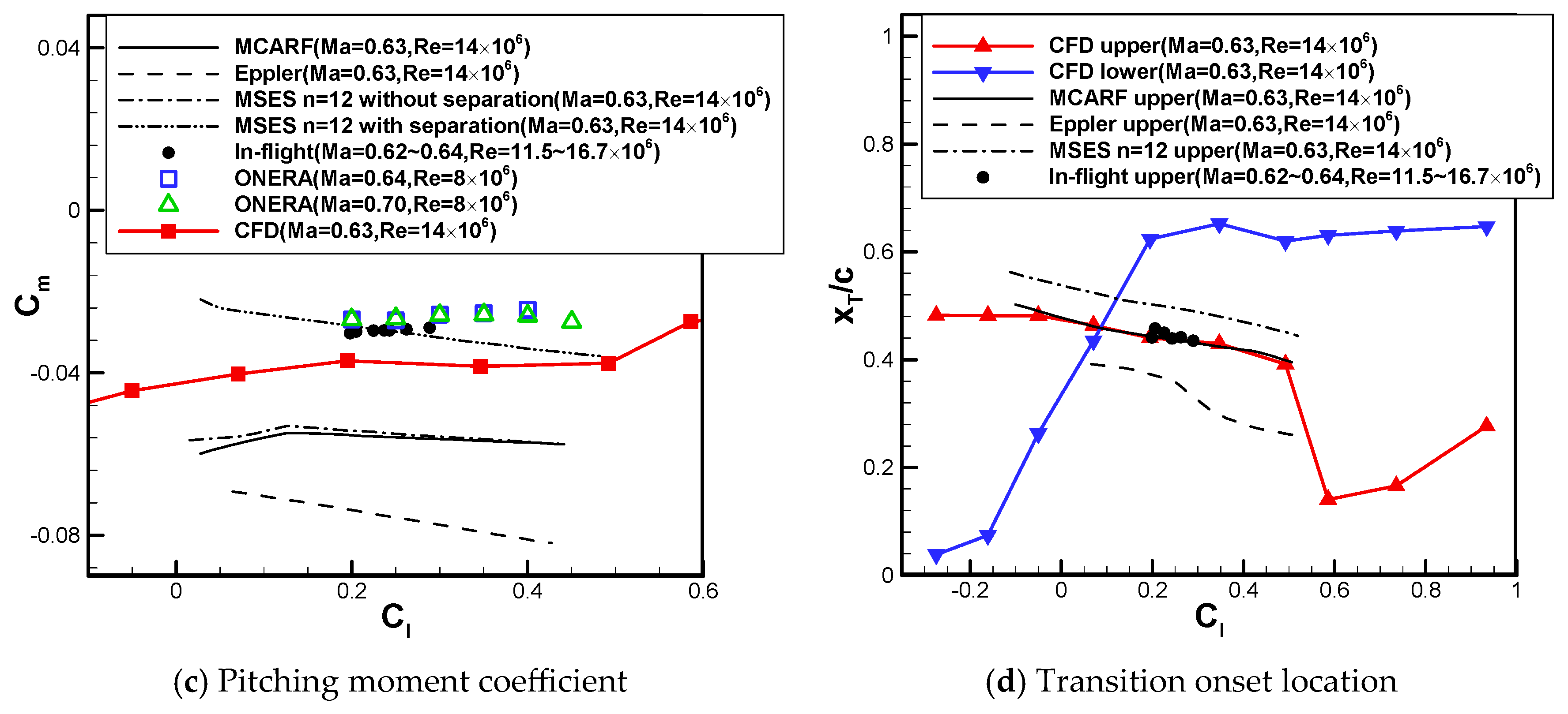
The Mach number for Case 1 falls within the subcritical regime, below the level of the typical cruise Mach number 0.69. Figure 12a displays the temperature of the wing upper surface captured via in-flight infrared photography, with the TOL roughly at x/c = 44%. The simulation results shown in Figure 12b support this, also indicating that the transition occurs near x/c = 63% on the lower surface, aligning with the designed laminar characteristics. For another case under subcritical conditions (Case 2), the predicted aerodynamic characteristics are fairly close to both in-flight and wind tunnel data, and generally fall within the range of other solvers’ results [6,26] (Figure 13a–c). Any deviations from experimental data may be due to variations in reconstructed airfoil shape or incompletely consistent with the flight/wind-tunnel conditions. Nonetheless, as shown in Figure 13d, the predicted TOLs on the upper surface match the flight test data well, again confirming the model’s fidelity at subcritical conditions.
Figure 12.
Comparison of predicted results with in-flight test for the SHM-1 airfoil at Ma = 0.6261, Re = 11.6 × 10⁶ and Cl = 0.2667 (Case 1). (a) Real-time wing surface temperature from infrared camera [26]; (b) comparison of predicted surface coefficient distributions with in-flight TOL.
Figure 13.
Comparison of predicted results with data from different sources for the SHM-1 airfoil at Ma = 0.63, Re = 14 × 106 and α = −4°~5° (Case 2).
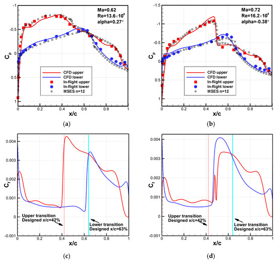
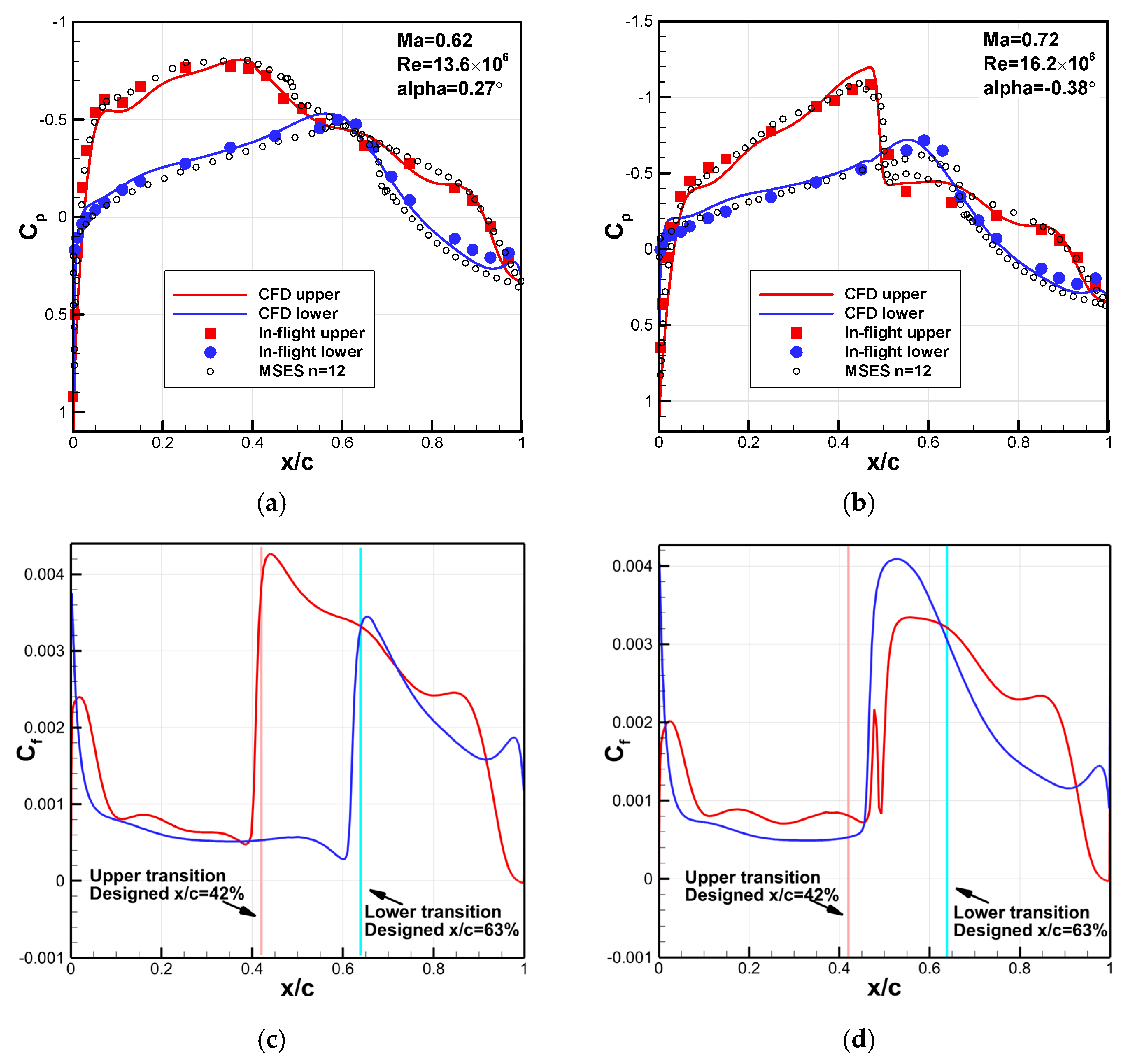
Based on Figure 14a,b, the transition model still reasonably predicts pressure patterns under subcritical (Case 3) and supercritical (Case 4) conditions, which is better than the results from the MSES solver. However, the predicted TOL (Figure 14d) differs significantly from the design expectation (Figure 14c) for supercritical conditions (Case 4), since both Mach and Reynolds numbers exceed the design values (Ma = 0.69, Re = 11.7 × 10⁶). The pressure coefficient distribution (Figure 14b) shows that the stronger favorable pressure gradient on the upper surface should delay transition. However, the intense shock wave causes fluctuations in skin friction, leading to a transition at that point (Figure 14d).
Figure 14.
Comparison of predicted results with in-flight test for the SHM-1 airfoil under subcritical and supercritical conditions. (a) Pressure coefficient distribution at Ma = 0.62, Re = 13.6 × 10⁶ and α = 0.27° (Case 3); (b) pressure coefficient distribution at Ma = 0.72, Re = 16.2 × 10⁶ and α = −0.38° (Case 4); (c) skin friction coefficient distribution at Ma = 0.62, Re = 13.6 × 10⁶ and α = 0.27° (Case 3); (d) skin friction coefficient distribution at Ma = 0.72, Re = 16.2 × 10⁶ and α = −0.38° (Case 4).
3.3. Effect of High Reynolds Number on Laminar Characteristics
Transition predictions for the NLF(1)-0416, HSNLF(1)-0213 and SHM-1 airfoils can also indicate the influence of higher Reynolds number on laminar characteristics for airfoil design. As the freestream Reynolds number of the NLF(1)-0416 airfoil rises from 4 × 10⁶ to 9 × 10⁶, the TOLs on both the upper and lower surfaces shift upstream by 10%~20%c across the entire range of computed angles of attack (Figure 8). For the HSNLF(1)-0213 airfoil, increasing the Reynolds number from 4 × 10⁶ to 11 × 106 results in minimal changes to the overall surface pressure distribution shape. Transition onset locations on both surfaces move upstream by about 10%c, yet laminar flow still extends over more than x/c = 50% (Figure 10). Regarding the SHM-1 airfoil in Figure 14, when flight conditions go beyond the design point to a supercritical state (Mach number rising from 0.62 to 0.72, Reynolds number from 13.6 × 10⁶ to 16.2 × 10⁶), a favorable pressure gradient remains on the upper surface. However, transition occurs due to shock wave formation. On the lower surface, transition also occurs earlier with increased Reynolds number, but the laminar flow region stays above x/c = 40%.
For laminar airfoil design, a consensus has been reached on the design concept [6,7], that a gentle favorable pressure gradient is retained from the leading edge to suppress the instabilities growth in the boundary layer, followed by a gently varying adverse pressure recovery to avoid flow separation. Using this kind of pressure distribution, for low-speed or transonic laminar airfoil design, higher Reynolds numbers do not fundamentally eliminate laminar flow characteristics based on the above findings. Notably, the compressibility effects of increased Mach number can enhance the boundary layer stability, making laminar characteristics robust against variations in Mach and Reynolds numbers.
4. Multi-Objective Aerodynamic Optimization
Based on the above validation and assessment results, the transition model is fully reliable for predicting high-speed and high-Reynolds-number boundary-layer transition. In this section, a multi-objective drag optimization is conducted for high-speed business jet laminar airfoil design. The HSNLF(1)-0213 airfoil is used as a baseline reference, and its performance is used to formulate the constraints. The design conditions are given based on the climb and cruise flight conditions of the SHM-1 airfoil, where the design AOA is calculated based on the lift design conditions (see Section 3.2).
4.1. Isight-Based Optimization Framework
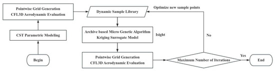
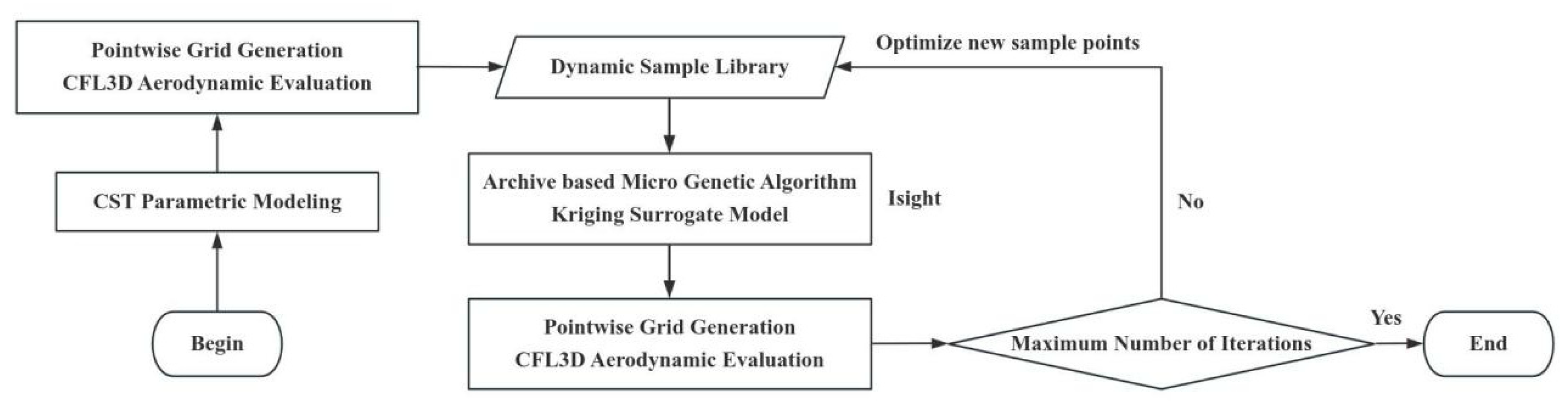
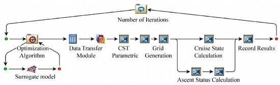
The optimization design framework built on the SIMULIA Isight platform [27] is shown in Figure 15. The class/shape function transformation (CST) method is used for airfoil shape parameterization. The structured mesh is generated using Pointwise v17.3 software and computed in parallel using the transition model in CFL3D solver for aerodynamic performance. Initial (dynamic) sample library is constructed through Latin hypercube sampling (LHS). In the Isight platform, the Archive-Based Micro Genetic Algorithm (AMGA) [28] is employed for optimization based on the variable-precision Kriging surrogate model. The newly optimized sample point is then added to the dynamic sample library after CFD evaluation. This library is used to construct a new surrogate model for the next round of optimization. The accuracy of the surrogate model continuously improves (i.e., variable-precision) as the dynamic sample library expands, accelerating optimization convergence toward the optimal solution. AMGA is a highly efficient variant of small-scale genetic algorithms. Its core feature lies in employing a micro-fixed population alongside an external archive to preserve historically superior solutions, thereby balancing the algorithm’s search capability with computational efficiency. During each iteration, local search is employed to refine the optimal solution, with high-performing individuals stored in the archive. When population diversity becomes insufficient, the algorithm reintroduces quality solutions from the archive to revitalize the search, effectively preventing premature convergence.
Figure 15.
Optimization design framework based on SIMULIA Isight platform.
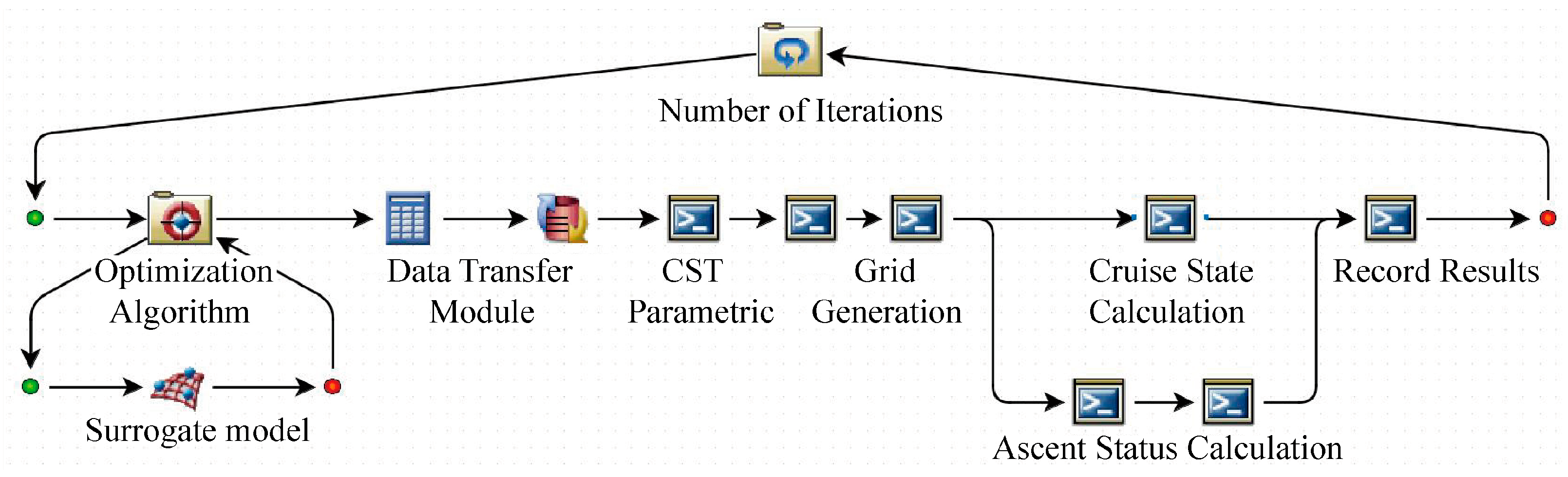
Figure 16 further illustrates the optimization design workflow in Isight. The optimization process runs cyclically based on a predetermined number of iterations, with its core being the loop of the optimization algorithm and surrogate model. This loop performs optimization searches using variable-precision surrogate models constructed from dynamic sample libraries. The optimal solution obtained from each optimization round enters the objective function evaluation process to obtain climb and cruise performances.
Figure 16.
Isight Platform Optimization Design Process.
4.2. Mathematical Model and Parameter Settings of Optimization
Setting HSNLF(1)-0213 as the baseline airfoil, lift/thickness-constrained multi-objective drag-reduction optimization was conducted for both climb (Ma = 0.31, Re = 13.6 × 10⁶ and α = 1.7°) and cruise (Ma = 0.69, Re = 11.7 × 10⁶ and α = 0.7°) flight conditions. The optimization mathematical model is shown in Equation (1). The baseline lift coefficients CL,climb = 0.31138 for climb condition and CL,cruise = 0.28936 for cruise condition, along with the maximum relative thickness t/c = 0.132, serve as constraints. The baseline HSNLF(1)-0213 airfoil has low-drag performance, being CD,climb = 0.00531 and CD,cruise = 0.00477, at climb and cruise conditions. Nine-order CST with respectively 10 parameters for the upper and lower surfaces of the airfoil are selected as design-variable vector xu and xl, with xui,max and xui,min and xli,max and xli,min denoting the upper and lower bounds of each design variable, where i = 0,1, …,9. The design space (i.e., variation range of each design variable) is set as ±10% disturbance around the baseline value.
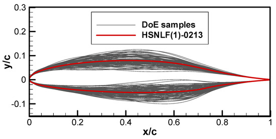
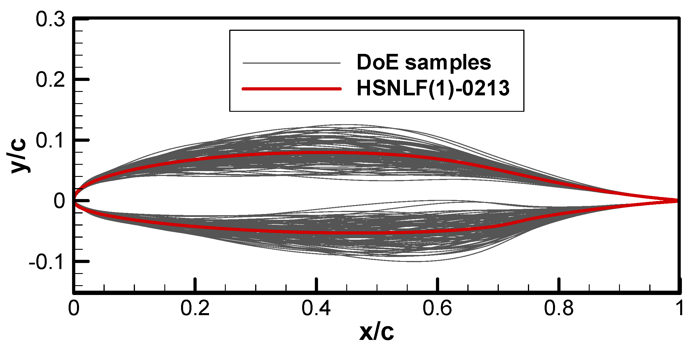
One hundred initial samples were firstly generated through the design of experiment (DoE) using Latin hypercube sampling (LHS). The airfoil shape of all the initial samples is integrated in Figure 17. The population size of AMGA was set to 40 with maximum 500 times function evaluations based on Kriging model in generation evolution. The archive size is limited to 500. The maximum number of optimization iteration is 200 with a Pareto solution set size of 100. In all the CFD evaluations, a freestream turbulence intensity of 0.03% was assumed with the viscosity ratio RT,inf = 5.0.
Figure 17.
All the initial samples by DoE using LHS.
4.3. Optimization Results and Discussion
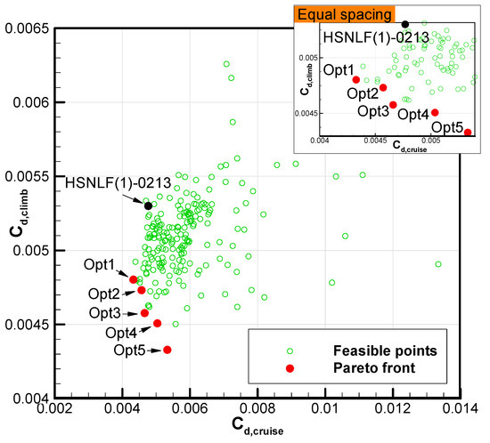
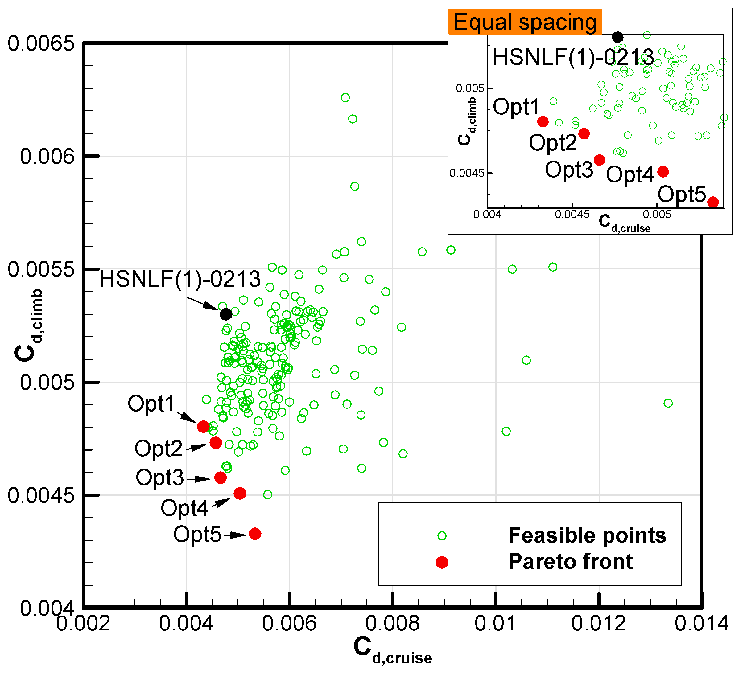
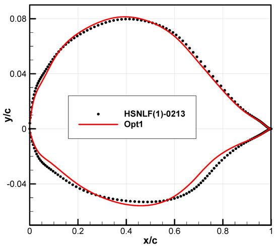
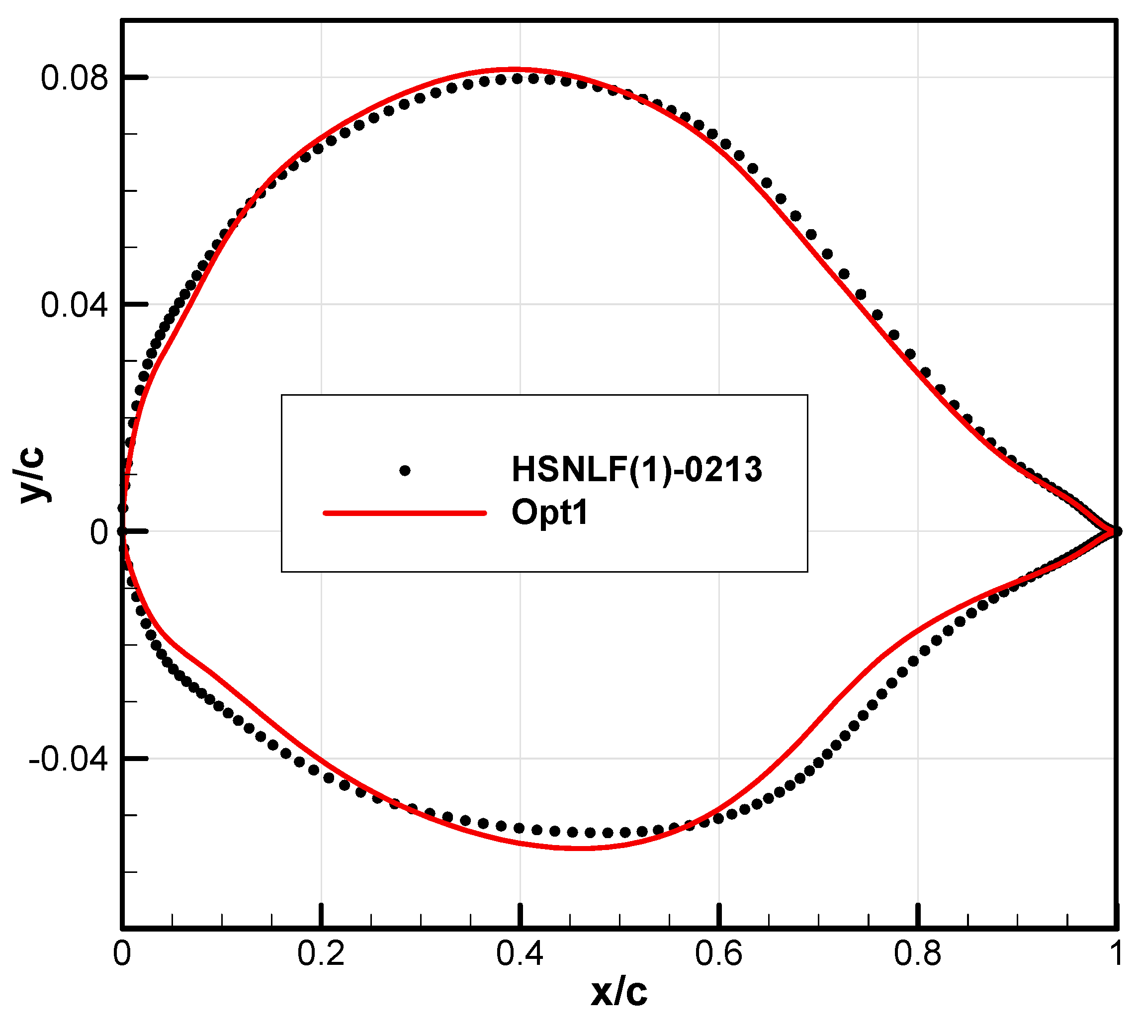
The multi-objective optimization result is shown in Figure 18; all solutions (marked by green circles) satisfy constraints and thus, are all feasible solutions. Red solid circles mark the Pareto frontier points, while the black solid circle is the drag performance of baseline HSNLF(1)-0213 airfoil. Due to changes in the cruise design conditions and considering the climb conditions simultaneously, the performance of the HSNLF(1)-0213 airfoil under the design conditions of this work is not optimal. Among all the Pareto frontier points, three marked designs with Opt1 to Opt3 are Pareto superior to the baseline. Although the climb drag of the Opt1 airfoil is not optimized, its cruise drag has been significantly improved. This can be seen from the enlarged diagram with equal spacing in Figure 18. Therefore, Opt1 was selected as the optimal design. The performance of Opt1 airfoil is CD,climb = 0.00480 and CD,cruise = 0.00433, with reductions of 9.53% and 9.21%, respectively, compared to the baseline values. After optimization, the lift not only meets the constraints but also increases slightly, resulting in a more significant improvement in the lift-drag ratio, with increases of 12.19% for climbing and 11.92% for cruising, respectively. The shape comparison between the optimized and baseline HSNLF(1)-0213 airfoil is shown in Figure 19. It can be observed that after optimization, the leading-edge radius is reduced, which lowers the leading-edge pressure peaks on both the upper and lower surfaces, mainly due to lift constraints. Subsequently, an obvious “concave” region appears on both the upper and lower surfaces within x/c = 0.05–0.1 from the leading edge. As can be seen from the following analysis of pressure distribution changes, this design exerts beneficial effects on both surfaces. The thickness of the optimized airfoil increases slightly to 0.137c, while the position of maximum thickness remains essentially unchanged (x/c = 0.42–0.43). The upper surface of the rear part is basically unchanged, but the lower surface exhibits obvious aft-loading characteristics to meet the lift constraint. This is similar to the SHM-1 airfoil (Figure 11b).
Figure 18.
Multi-objective optimization results with Pareto front and baseline reference.
Figure 19.
Shape comparison before and after optimization.
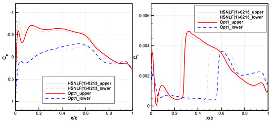
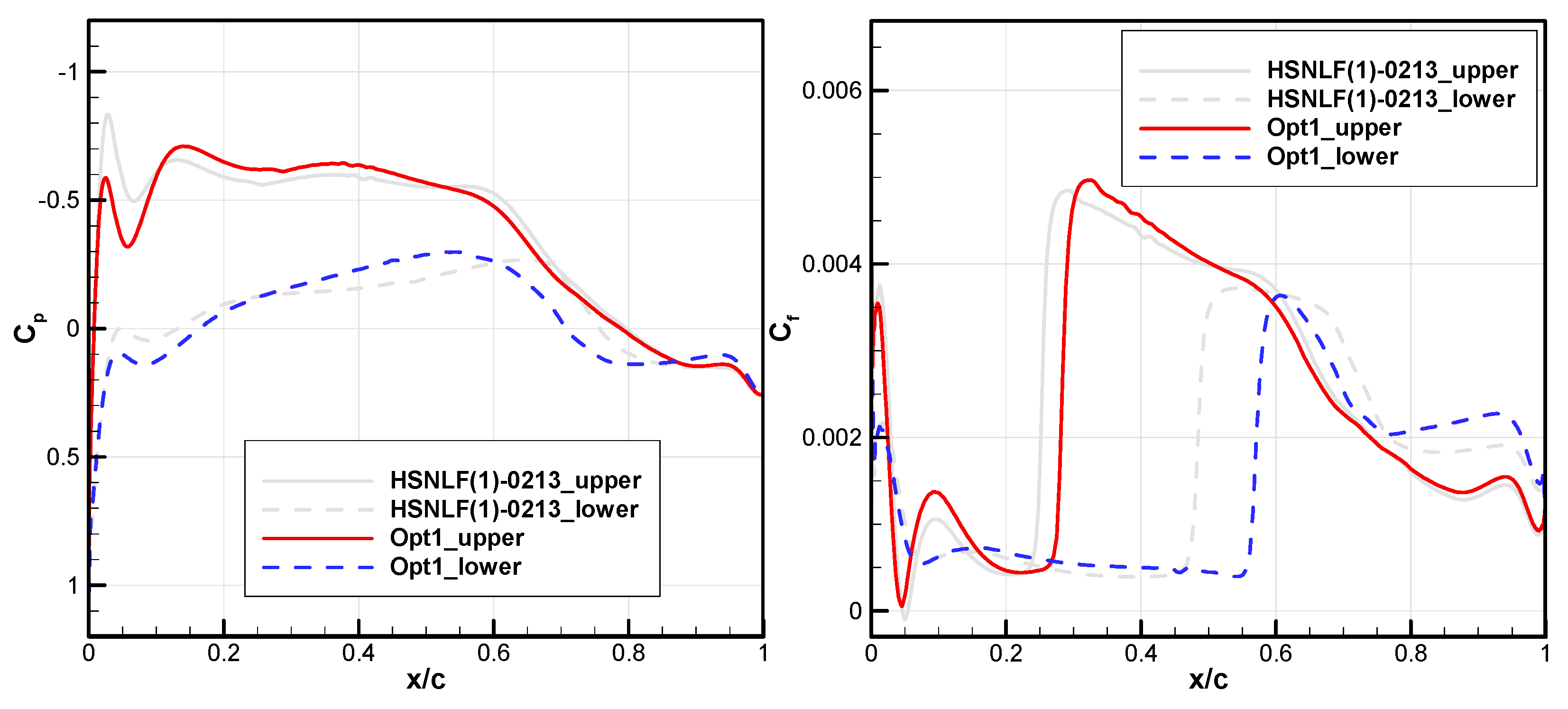
A comparison of pressure coefficients and skin friction coefficients at climb conditions is shown in Figure 20, where solid lines represent the upper surface and dashed lines represent the lower surface. For the upper surface of optimized airfoil, the aforementioned “concave” region reduces the leading-edge suction peak and prevents possible transition induced by the separation bubble, which is present at x/c = 0.05 of the HSNLF(1)-0213 airfoil. The subsequent pressure distribution pattern does not change significantly. The slightly gentler adverse pressure gradient of the optimized airfoil causes the transition position to move slightly downstream from x/c = 0.25 to 0.3. For the lower surface of optimized airfoil, the “concave” region generates larger pressure near the leading edge, providing a pressure difference reserve for a subsequent wide range of favorable pressure gradients while satisfying lift constraints. In contrast, HSNLF(1)-0213 airfoil does not sustain a continuous favorable pressure gradient within this range. This delays the TOL from x/c = 0.5 of the baseline airfoil to x/c = 0.6 of the optimized one. From the relationship between the pressure distribution patterns and TOLs on both upper and lower surfaces, it can be concluded that a favorable pressure gradient is essential for maintaining laminar flow at high Reynolds numbers (Re = 13.6 × 10⁶). In addition, the aft-loading phenomenon of optimized airfoil is obviously required to meet the constraint of lift.
Figure 20.
Comparison of pressure and skin friction coefficient at climb conditions.
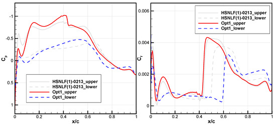
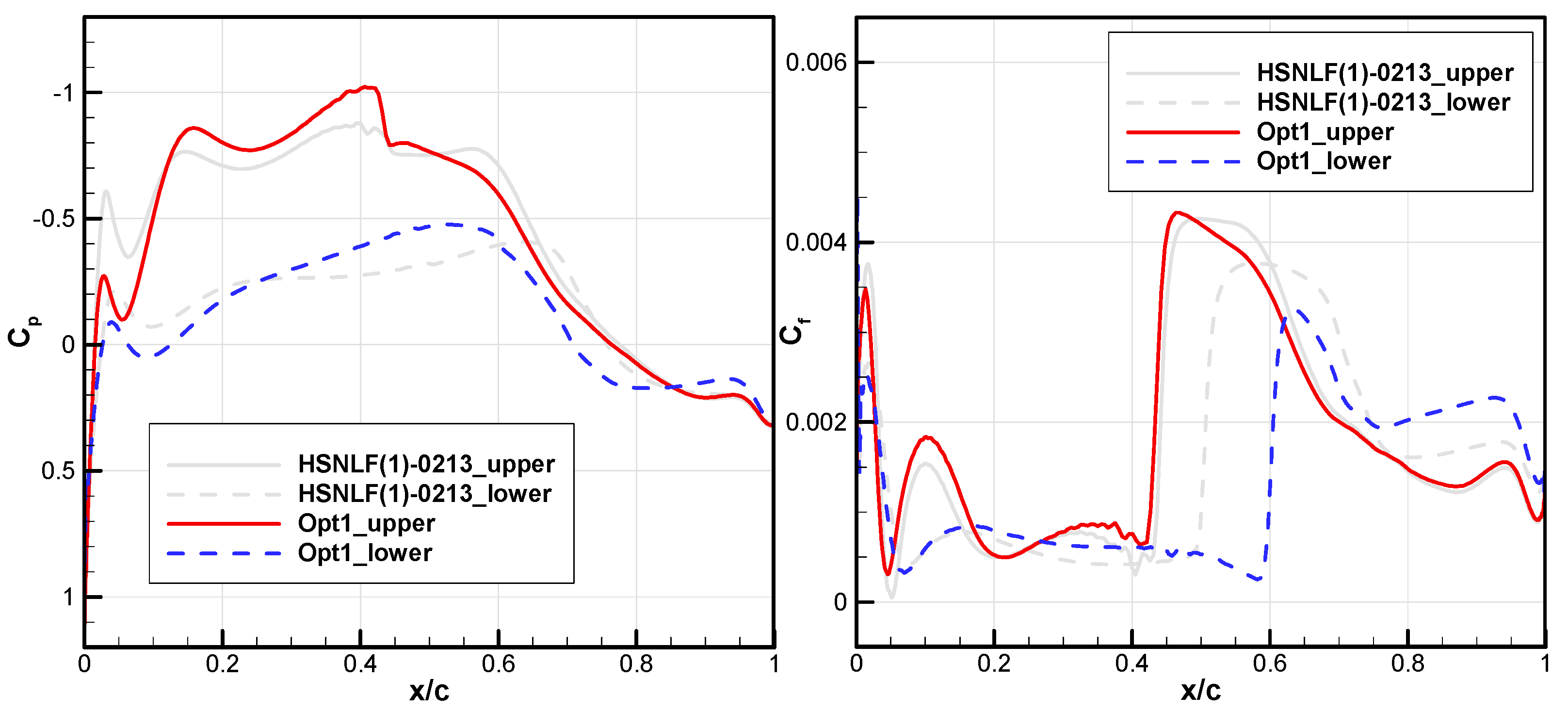
A comparison of pressure coefficients and skin friction coefficients at cruise condition is shown in Figure 21. Since the AOA under cruise condition vary significantly from the design conditions of the HSNLF(1)-0213 airfoil itself (around α = −0.953°), the pressure distribution under cruise conditions also differs significantly from that in Figure 10. At this time, the TOL on the upper surface of the optimized airfoil remains basically unchanged at x/c = 0.45, even moving upstream slightly, and a weak shock wave is generated due to a lower suction peak and strong pressure recovery to meet the life constraint. In contrast, due to the same mechanism as for the climb condition (a widely ranging favorable pressure gradient due to the “concave” region), the lower surface exhibits a strong accelerating flow up to x/c = 0.55. This allows the laminar flow to be maintained until about x/c = 0.6. Since the TOL on the lower surface of the optimized airfoil is more downstream, the friction drag is much smaller, which offsets the impact of shock-wave drag, resulting in a decrease in total cruise drag.
Figure 21.
Comparison of pressure and skin friction coefficient at cruise conditions.
Overall, whether in low-speed or high-speed conditions, the maintenance of laminar flow at higher Reynolds numbers requires a more favorable pressure gradient than under lower Reynolds number conditions. This is consistent with the ideal pressure distribution pattern obtained in Section 3.3. In addition, a special shape appears in this case, namely the leading-edge “concave” region. According to the optimization results, on the upper surface, this region can prevent possible transitions caused by local separation bubbles. However, an excessively low suction peak imposes a burden on lift maintenance (thus, aft-loading is essential), and could form a shock wave due to strong pressure recovery at high speed, which weakens the overall drag reduction benefit. On the lower surface, it can provide a considerable pressure difference reserve, generate a wide range of favorable pressure gradient, and significantly delay the TOL.
5. Conclusions
Based on a detailed prediction fidelity assessment of the transition model under high-speed actual flight conditions with a high Reynolds number, this paper conducts a multi-objective drag-reduction optimization on a high-speed business jet laminar airfoil, considering climb and cruise conditions. The main conclusions are as follows:
- (1)
- Validation with the AIAA TMPW-1 standard test case, e.g., the NLF(1)-0416 airfoil, shows that the transition model converges well with grid refinement. It is concluded that a fine mesh can offer adequate resolution.
- (2)
- For high Reynolds numbers above 107, e.g., the HSNLF(1)-0213 and SHM-1 high-speed laminar airfoils, the transition model also demonstrates reliable predictive accuracy for natural transitions and transitions caused by small separation bubbles. The prediction results show satisfactory agreement with design expectations, experimental observations or flight tests, which strongly confirms the effectiveness of the transition model at transonic flight conditions.
- (3)
- Higher Reynolds numbers do not fundamentally eliminate laminar flow characteristics. In other words, the aerodynamic advantages of laminar flow at the design point are not entirely lost with moderate increases in Reynolds number.
- (4)
- The multi-objective optimization based on the fully assessed transition model yields an optimal airfoil with 9.53% climb drag reduction and 9.21% cruise drag reduction. The result demonstrates that aft-loading with wide range of favorable pressure gradients is essential to sustain extensive laminar flow and balance lift, which offers a validated engineering design framework for high-speed business jet laminar airfoils under high-Reynolds-number flight conditions.
Author Contributions
Conceptualization, Y.D. and J.Y.; methodology, Y.D. and B.Z.; software, B.Z.; validation, Q.X.; formal analysis, J.Y. and B.Z.; investigation, Y.D. and J.Y.; resources, H.Z.; data curation, J.Y., H.Z. and Q.X.; writing—original draft preparation, Y.D. and J.Y.; writing—review and editing, Y.D.; visualization, Y.D. and B.Z.; supervision, Y.D.; project administration, Y.D.; funding acquisition, Y.D. All authors have read and agreed to the published version of the manuscript.
Funding
This research was funded by National Natural Science Foundation of China with grant number 12202284.
Institutional Review Board Statement
Not applicable.
Informed Consent Statement
Not applicable.
Data Availability Statement
The original contributions presented in this study are included in the article. Further inquiries can be directed to the corresponding author.
Conflicts of Interest
The authors declare no conflict of interest.
References
- Li, J.; Zhao, Y.; Wang, W.; Xie, L.; Zhang, H.; Wang, L.; Yuan, L.; Tan, Y.; Ning, Y. Overall Aerodynamic Technology Challenges and Development Prospects for the Next-Generation Supersonic Transport. Acta Aeronaut. Astronaut. Sin. 2025, 46, 532069. (In Chinese) [Google Scholar] [CrossRef]
- Sun, Y.; Smith, H. Review and prospect of supersonic business jet design. Prog. Aerosp. Sci. 2017, 90, 12–38. [Google Scholar] [CrossRef] [Scilit]
- Hua, J.; Zhong, M.; Zheng, S.; Wang, G.; Wang, H.; Bai, J. Design and database applications of CAE-AVM model cruise configuration. Acta Aerodyn. Sin. 2022, 40, 133–147. (In Chinese) [Google Scholar] [CrossRef]
- Yuan, J.; Sun, J.; Li, L.; Yu, S.; Nie, H.; Gao, L.; Han, Z.; Qian, Z. Progress of supersonic aircraft laminar flow layout design and evaluation technologies. Acta Aeronaut. Astronaut. Sin. 2022, 43, 526316. (In Chinese) [Google Scholar] [CrossRef]
- Dornier 228 Advanced Commuter (AC) Facts & Figures. RUAG Aerospace Services GmbH. Available online: https://www.dornier228.com (accessed on 4 April 2026).
- Fujino, M. Design and Development of the HondaJet. J. Aircr. 2005, 42, 755–764. [Google Scholar] [CrossRef] [Scilit]
- Thomas, B. ‘Wonderment’ Defined—UP.Summit Showcases Mobility Advancements. Aircraft Owners and Pilots Association (AOPA). 2 October 2025. Available online: https://aopa.org/news-and-media/all-news/2025/october/02/wonderment-defined# (accessed on 4 April 2026).
- Whitney, J. Phantom 3500 Swaps Windows for Super-Efficient Transonic Flight. Military + Aerospace Electronics. 20 May 2025. Available online: https://www.militaryaerospace.com/commercial-aerospace/article/55291318/phantom-3500-swaps-windows-for-super-efficient-transonic-flight (accessed on 4 April 2026).
- Chen, Y.; Wang, S.; Liu, W. Data-Driven Transition Models for Aeronautical Flows with a High-Order Numerical Method. Aerospace 2022, 9, 578. [Google Scholar] [CrossRef] [Scilit]
- Shi, Y.; Song, C.; Chen, Y.; Rao, H.; Yang, T. Complex standard eigenvalue problem derivative computation for laminar–turbulent transition. AIAA J. 2023, 61, 3404–3418. [Google Scholar] [CrossRef] [Scilit]
- Zhao, Z.; Chen, X.; Wang, L.; Fu, S. Evolution and development of flow transition and supersonic modes under high-temperature gas effects. Acta Aerodyn. Sin. 2024, 42, 75–83. (In Chinese) [Google Scholar] [CrossRef]
- Menter, F.; Langtry, R.; Likki, S.; Suzen, Y.; Huang, P.; Völker, S. A Correlation Based Transition Model Using Local Variables Part 1: Model Formulation. ASME J. Turbomach. 2006, 128, 413–422. [Google Scholar] [CrossRef] [Scilit]
- Langtry, R.; Menter, F. Correlation-Based Transition Modeling for Unstructured Parallelized Computational Fluid Dynamics Codes. AIAA J. 2009, 47, 2894–2906. [Google Scholar] [CrossRef] [Scilit]
- Catalano, P.; Tognaccini, R. RANS analysis of the low-Reynolds number flow around the SD7003 airfoil. Aerosp. Sci. Technol. 2011, 15, 615–626. [Google Scholar] [CrossRef] [Scilit]
- Wang, Y.; Zhang, Y.; Li, S.; Meng, D. Calibration of a transition model and its validation in low-speed flows with high-order numerical method. Chin. J. Aeronaut. 2015, 28, 704–711. [Google Scholar] [CrossRef] [Scilit]
- Lampropoulos, N.K.; Sarris, I.E.; Antoniou, S.; Ziogas, O.; Panagiotou, P.; Yakinthos, K. Aerodynamic Performance of a Natural Laminar Flow Swept-Back Wing for Low-Speed UAVs Under Take Off/Landing Flight Conditions and Atmospheric Turbulence. Aerospace 2025, 12, 934. [Google Scholar] [CrossRef] [Scilit]
- Robitaille, M.; Mosahebi, A.; Laurendeau, É. Design of adaptive transonic laminar airfoils using the transition model. Aerosp. Sci. Technol. 2015, 46, 60–71. [Google Scholar] [CrossRef] [Scilit]
- AIAA Transition Modeling and CFD Vision 2030, NASA Langley Research Center. Available online: http://transitionmodeling.larc.nasa.gov (accessed on 4 April 2026).
- The Langtry-Menter 4-Equation Transitional SST Model, Turbulence Modeling Resource. Available online: https://turbmodels.larc.nasa.gov/langtrymenter_4eqn.html (accessed on 4 April 2026).
- Krist, S.; Biedron, R.; Rumsey, C. CFL3D User’s Manual-Ver. 5.0, 2nd ed.; NASA Langley Research Center: Hampton, VA, USA, 1998. Available online: https://ntrs.nasa.gov/api/citations/19980218172/downloads/19980218172.pdf (accessed on 4 April 2026).
- Spalart, P.; Rumsey, C. Effective Inflow Conditions for Turbulence Models in Aerodynamic Calculations. AIAA J. 2007, 45, 2544–2553. [Google Scholar] [CrossRef] [Scilit]
- Somers, D. Design and Experimental Results for a Natural-Laminar Flow Airfoil for General Aviation Applications; NASA-TP-1861; NASA Technical Publication: Washington, DC, USA, 1981.
- Coder, J. Standard Test Cases for Transition Model Verification and Validation in Computational Fluid Dynamics. In Proceedings of the 2018 AIAA Aerospace Sciences Meeting, Kissimmee, FL, USA, 8–12 January 2018. [Google Scholar]
- Viken, J.; Viken, S.; Pfenninger, W.; Morgan, H., Jr.; Campbell, R. Design of the Low Speed NLF(1)-0414F and the High Speed HSNLF(1)-0213 Airfoils with High-Lift Systems. In Research in Natural Laminar Flow and Laminar-Flow Control; NASA CP-2487 Part 3; National Aeronautics and Space Administration (NASA): Washington, DC, USA, 1987; pp. 637–671. [Google Scholar]
- Viken, J. Boundary-Layer Stability and Airfoil Design. In Laminar Flow Aircraft Certification; NASA-CP-2413; NASA Langley Research Center: Hampton, VA, USA, 1985; pp. 1–30. [Google Scholar]
- Fujino, M.; Yoshizaki, Y.; Kawamura, Y. Natural-Laminar-Flow Airfoil Development for a Lightweight Business Jet. J. Aircr. 2003, 40, 609–615. [Google Scholar] [CrossRef] [Scilit]
- Tian, Y.; Quan, J.; Liu, P.; Li, D.; Kong, C. Mechanism/structure/aerodynamic multidisciplinary optimization of flexible high-lift devices for transport aircraft. Aerosp. Sci. Technol. 2019, 93, 104813. [Google Scholar] [CrossRef] [Scilit]
- Tiwari, S.; Koch, P.; Fadel, G.; Deb, K. AMGA: An archive-based micro genetic algorithm for multi-objective optimization. In Proceedings of the 10th Annual Conference on Genetic and Evolutionary Computation, Atlanta, GA, USA, 12–16 July 2008; pp. 729–736. [Google Scholar] [CrossRef] [Scilit]

Disclaimer/Publisher’s Note: The statements, opinions and data contained in all publications are solely those of the individual author(s) and contributor(s) and not of MDPI and/or the editor(s). MDPI and/or the editor(s) disclaim responsibility for any injury to people or property resulting from any ideas, methods, instructions or products referred to in the content. |
© 2026 by the authors. Licensee MDPI, Basel, Switzerland. This article is an open access article distributed under the terms and conditions of the Creative Commons Attribution (CC BY) license.