An Online Trajectory Optimization Method for the TAEM Phase Based on an Analytical Lateral Path and Equivalent Dynamic Decoupling

Abstract

Rapid and robust trajectory planning for the Terminal Area Energy Management (TAEM) phase of horizontal-landing Reusable Launch Vehicles (RLVs) is critical but challenging due to large initial deviations, stringent terminal constraints, and strong model nonlinearities. To address the limitations of existing methods in convergence reliability and computational speed, this paper proposes a novel online trajectory optimization framework based on analytical lateral planning and equivalent dynamic decoupling. First, a cubic Bézier curve is employed to parameterize the lateral ground track, enabling the rapid generation of analytical expressions for the lateral states that strictly satisfy boundary constraints. Leveraging these analytical solutions, the original six-degree-of-freedom dynamics are exactly decoupled and reduced to a lower-dimensional model governing only the longitudinal motion. To further mitigate nonlinearity, the third derivative of height with respect to range is introduced as a virtual control variable, transforming the problem into a smoother form. The resulting equivalent longitudinal optimization problem is then efficiently solved using the Gauss Pseudospectral Method. Numerical simulations demonstrate that the proposed method significantly outperforms traditional approaches in computational efficiency: it generates feasible trajectories satisfying all constraints within 0.26 s (3$\sigma$ value). Furthermore, the method exhibits remarkable insensitivity to initial guesses, achieving stable convergence even with simple linear initialization. This approach provides a robust and real-time capable solution for complex TAEM trajectory optimization problems characterized by high nonlinearity and multiple constraints.

1. Introduction

The new generation of RLV, typically utilizing a lifting-body configuration, possesses the capability to traverse the dense atmosphere, near space, and low Earth orbit. This enables low-cost, high-efficiency orbital delivery and ultra-long-range cargo transportation [1,2], garnering widespread attention in the aerospace community. Upon mission completion, an RLV re-enters the atmosphere and executes a precision landing at a designated airport, akin to an aircraft, thereby reducing launch costs through reusability. The vehicle’s unique lifting-body geometry provides superior aerodynamic performance, facilitating extensive lateral maneuvering and high-precision trajectory control during reentry, which enhances both deployment flexibility and recovery capabilities. Moreover, the ability to operate from conventional airports eliminates reliance on specialized launch and landing infrastructure. Compared to traditional expendable launch systems, RLV offers distinct advantages in terms of cost-effectiveness, reliability, and operational responsiveness [3,4]. However, realizing these benefits relies heavily on the generation of feasible and robust flight paths, making trajectory planning a determinant factor for mission success. Consequently, advanced research into RLV trajectory design, guidance, and control has emerged as a critical focal point in recent years.

The reentry trajectory of an RLV typically comprises three distinct phases: the Initial Re-entry (IRE) phase, the Terminal Area Energy Management (TAEM) phase, and the Approach and Landing (A&L) phase [5]. Among these, the TAEM phase represents one of the most critical and challenging phases of the return mission. During this phase, the vehicle must glide under unpowered conditions, relying solely on the modulation of the angle of attack and bank angle to precisely guide six state variables—height, velocity, position, heading angle, and flight path angle—to the stringent entry corridor of the Approach and Landing Interface (ALI). The inherent complexities arising from multiple path constraints, strong dynamic nonlinearities, and the underactuated nature of the vehicle present significant technical hurdles for online trajectory planning [6]. Consequently, the development of autonomous, precise, and robust online trajectory planning algorithms is paramount for ensuring the safe and efficient reuse of RLVs.

The baseline strategy for trajectory planning in the RLV TAEM phase was established by the Space Shuttle program [7], which decouples the reference trajectory into separate longitudinal and lateral profiles. The lateral ground track is geometrically constructed by splicing distinct segments—namely, the acquisition phase, straight-line flight, heading alignment cone, and pre-final phase—to satisfy terminal constraints. Longitudinally, the trajectory is defined by energy and height profiles, which are tracked during flight by modulating the angle of attack and speed brake, while the bank angle controls the lateral path. Building upon this pioneering framework, subsequent research has focused on enabling online planning capabilities. Kluever et al. [8,9] significantly reduced the computational burden by simplifying the planning problem into the online solution of a few key geometric parameters. Further advancements have introduced techniques such as the energy-tube concept [10], dynamic pressure protection method [11], Equivalent Wings Level Range [12], the Energy Dissipation Circle (EDC) [13], and sliding mode control theory [14] and so on [15,16,17]. These developments have, to a certain extent, improved computational efficiency and adaptability to initial state deviations. However, such methods suffer from inherent limitations, including the lack of optimality in longitudinal profiles, the rigidity of fixed lateral ground tracks, and the complexity of piecewise logic design, making them difficult to adapt to complex and variable flight scenarios.

To overcome the limitations of planning methods in adaptability and optimality, researchers have extensively investigated numerical trajectory optimization techniques [18]. Various approaches have been explored for the TAEM phase, including combining direct transcription with differential flatness [19], integrating the Gauss pseudospectral method with the direct shooting method [20], Chebyshev pseudospectral methods [21], and applying pseudospectral methods augmented with feedback linearization [22]. However, these nonlinear optimization strategies generally suffer from low computational efficiency, rendering them unsuitable for onboard applications. With the emergence of convex optimization theory, some scholars have applied convexification techniques to trajectory planning for TAEM. Convex optimization is highly promising for online implementation due to its fast computation. However, its practical onboard application is still hindered by its high sensitivity to the initial guess and the heavy computational burden of solving complex formulations. Considering the limited processing power of current On-Board Computers (OBCs), these drawbacks can significantly degrade convergence reliability. Therefore, exploring alternative real-time methods that are robust and computationally lightweight remains necessary.

Synthesizing the limitations of existing approaches reveals a fundamental trade-off in TAEM trajectory planning: between real-time feasibility and trajectory optimality. On the one hand, traditional planning methods, characterized by their structured design and low computational load, have inherent potential for online application; however, their lack of optimality and limited adaptability fail to fully exploit the vehicle’s maneuvering capabilities. On the other hand, while numerical optimization methods excel in handling complex constraints and seeking optimal solutions, their prohibitive computational costs make it difficult to break free from the conventional paradigm of ‘offline design followed by online tracking’. Addressing this conflict by developing a novel methodology that simultaneously achieves real-time performance, optimality, and high adaptability represents a critical challenge that urgently needs to be resolved.

To address these challenges, this paper proposes a novel online trajectory optimization framework based on analytical lateral planning and equivalent dynamic decoupling. The methodology begins by utilizing a cubic Bézier curve to parameterize the lateral ground track. Analytical expressions for the lateral position, heading angle, and curvature are derived directly from the initial states and terminal constraints. These analytical solutions are then substituted into the vehicle’s dynamic equations, rigorously reducing the original six-degree-of-freedom system to a three-dimensional model. Furthermore, the third derivative of height with respect to range is introduced as a new virtual control variable to mitigate the longitudinal dynamics’ nonlinearity further. Finally, the Gauss Pseudospectral Method (GPM) is employed to solve the simplified optimization problem efficiently. Numerical simulations are conducted to validate the effectiveness, adaptability, and computational efficiency of the proposed method.

The main contributions of this work are summarized as follows:

(1) A cubic Bézier curve is innovatively employed to design the lateral trajectory, enabling the rapid derivation of analytical expressions for lateral states and curvature based on boundary conditions. This approach not only enhances the flexibility and adaptability of the path planning but also effectively circumvents the discontinuity issues in the heading angle rate inherent in traditional geometric splicing methods.

(2) By leveraging the analytical lateral solutions, the complex coupled dynamics are equivalently reduced to a simplified model governing only the longitudinal motion. Additionally, designing the third derivative of height with respect to range as the control variable significantly lowers the problem’s dimensionality and nonlinearity. These improvements drastically enhance computational efficiency and reduce sensitivity to initial guesses, thereby making the online application of GPM-based trajectory optimization feasible.

The remainder of this paper is organized as follows. Section 2 establishes the vehicle’s point-mass dynamics model. Section 3 details the analytical parameterization of the lateral motion using a cubic Bézier curve, which enables the equivalent decoupling of lateral and longitudinal dynamics and achieves the primary dimensionality reduction. In Section 4, a virtual control variable is introduced to simplify the longitudinal dynamics further, thereby formulating an optimization problem suitable for rapid solution. Section 5 offers the numerical simulation and analysis. Finally, Section 6 concludes the paper.

2. Description of TAEM Trajectory Planning Problem

During the TAEM phase of an RLV’s reentry mission, the flight range is relatively short, rendering the effects of Earth’s rotation and curvature negligible for trajectory planning purposes [8]. Furthermore, compared to the initial reentry phase, TAEM guidance places greater emphasis on the relative position and velocity between the vehicle and the landing site. Consequently, an airport-fixed coordinate system is established to describe the vehicle’s motion. Unlike the Earth-centered coordinate systems used in earlier orbital or reentry phases, this local frame is specifically adopted for the TAEM phase because it allows for direct and convenient formulation of terminal alignment constraints relative to the runway. The origin of this coordinate system is located at the runway threshold. The x-axis is aligned with the runway centerline, pointing in the direction of the landing approach; the y-axis is perpendicular to the x-axis and points vertically upwards; and the z-axis completes the right-handed system.

The vehicle’s equations of motion in the airport-fixed coordinate system are as follows:

$$\left\{\begin{array}{cc}\hfill \dot{x}=& Vcos\gamma cos\psi \hfill \\ \hfill \dot{y}=& Vsin\gamma \hfill \\ \hfill \dot{z}=& Vcos\gamma sin\psi \hfill \\ \hfill \dot{V}=& {\displaystyle \frac{-D}{m}}-gsin\gamma \hfill \\ \hfill \dot{\gamma }=& {\displaystyle \frac{L}{mV}}cos\sigma -{\displaystyle \frac{g}{V}}cos\gamma \hfill \\ \hfill \dot{\psi }=& {\displaystyle \frac{L}{mVcos\gamma }}sin\sigma \hfill \\ \hfill \dot{S}=& Vcos\gamma \hfill \end{array}\right.$$

(1)

where V is the magnitude of the velocity, $\gamma$ is the flight path angle, defined as the angle between the velocity vector and the $xoz$-plane, positive upwards. $\psi$ is the heading angle, defined as the angle between the projection of the velocity vector onto the $xoz$-plane and the x-axis, positive counter-clockwise. x, y and z are the position coordinates in the airport-fixed frame, with y equal to height h. In this paper, the term ‘height’ (h) refers to the vertical distance relative to the runway threshold level (i.e., altitude above field elevation), unless otherwise specified. $\sigma$ is the bank angle, $\alpha$ is the angle of attack, m is the mass, g represents the acceleration of gravity, and its value is set to 9.8 m/s², L and D are the lift and drag forces, respectively, which can be calculated using the following formulas

$$\begin{array}{cc}\hfill L=& q{S}_{\mathrm{ref}}{C}_L\hfill \\ \hfill D=& q{S}_{\mathrm{ref}}{C}_D\hfill \end{array}$$

(2)

where q is the dynamic pressure, $S_{\mathrm{ref}}$ is the characteristic area, $C_L$ and $C_D$ represent the aerodynamic lift coefficient and drag coefficient concerning angle of attack $\alpha$ and Mach number Ma.

TAEM constraints include path constraints and terminal state constraints. The path constraints are given by

$$\begin{array}{cc}\hfill q=& {\displaystyle \frac{1}{2}}\rho V^2<q_{max}\hfill \\ \hfill \dot{Q}=& k_Q{\rho }^{0.5}{V}^{3.15}\le {\dot{Q}}_{max}\hfill \\ \hfill n=& \sqrt{L^2+D^2}\le n_{max}\hfill \end{array}$$

(3)

where q, $\dot{Q}$, and n are the dynamic pressure, the heating rate and the aerodynamic load, $q_{max}$, ${\dot{Q}}_{max}$ and $n_{max}$ are the prescribed maximum limits on the dynamic pressure, the heating rate and the aerodynamic load respectively, $\rho$ is the atmospheric density, which is calculated using the 1976 U.S. Standard Atmosphere model, $k_Q$ is the heat transfer coefficient.

The constraints of terminal states and flight time are set as

$$\begin{array}{c}x=x_f,y=y_f,z=z_f\hfill \\ V=V_f,\gamma ={\gamma }_f,\psi ={\psi }_f.\hfill \end{array}$$

(4)

3. Lateral Trajectory Design and Model Decoupling Based on Bézier Curve

Direct trajectory optimization for RLVs faces significant challenges related to high computational loads and convergence difficulties. To mitigate these issues and reduce the problem scale, this section introduces a novel methodology combining Bézier-curve-based lateral trajectory design with equivalent dynamic decoupling. The procedure unfolds as follows: First, in Section 3.1, a feasible lateral ground track is parameterized using a cubic Bézier curve, yielding analytical solutions for the lateral states. Subsequently, in Section 3.2, these analytical solutions are substituted into the governing equations to derive closed-form expressions for the bank angle and lift force required to track the lateral path. Furthermore, the third derivative of height with respect to range is introduced as a virtual control variable to streamline the dynamics further. Through these analytical simplifications, the original six-state dynamic model is reduced to a three-state model. All variables, except for the primary longitudinal states, are expressed analytically, thereby significantly reducing the complexity of the subsequent trajectory optimization problem.

3.1. Lateral Trajectory Design Based on Bézier Curve

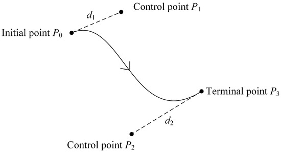
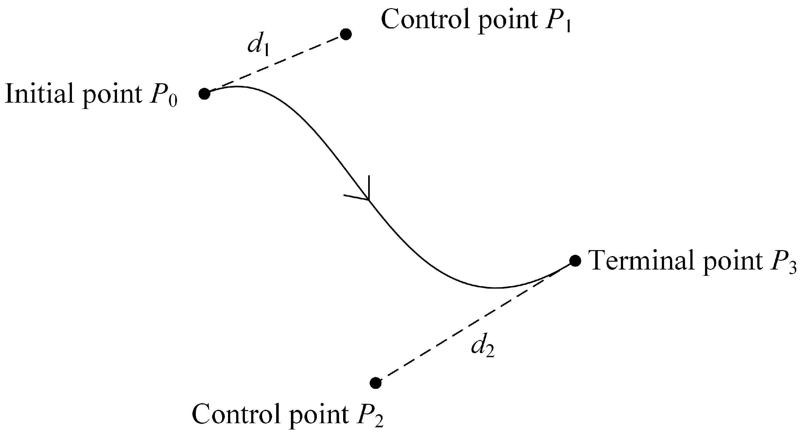
The primary objective of this section is to achieve the decoupling of lateral and longitudinal dynamics by obtaining an analytical representation of the lateral trajectory. To achieve this goal, the chosen parametric curve must simultaneously satisfy the requirements for matching boundary conditions and ensuring trajectory quality. The cubic Bézier curve demonstrates unique advantages in both of these aspects. First, regarding boundary conditions, the planning of the vehicle’s lateral trajectory is constrained by four boundary conditions: the initial position $\left(x_0,z_0\right)$, initial heading ${\psi }_0$, final position $\left(x_f,z_f\right)$, and final heading ${\psi }_f$. A cubic Bézier curve can satisfy these four boundary conditions and also allows for control over the curvature radii at the start and end points of the path, ensuring that the lateral trajectory complies with the vehicle’s flight capability constraints. Second, in terms of trajectory quality, a cubic Bézier curve possesses sufficient degrees of freedom to generate various smooth turning trajectories, from straight lines to S-shaped curves, which is adequate to cover the vast majority of reasonable flight paths in the TAEM phase. The shape of a cubic Bézier curve is illustrated in Figure 1.

Figure 1. Illustration of a cubic Bézier curve.

A cubic Bézier curve is determined by four points: ${\mathbf{P}}_0$, ${\mathbf{P}}_1$, ${\mathbf{P}}_2$, and ${\mathbf{P}}_3$. Here, ${\mathbf{P}}_0$ and ${\mathbf{P}}_3$ are the start and terminal points of the curve, respectively, while ${\mathbf{P}}_1$ and ${\mathbf{P}}_2$ are two adjustable control points. The direction of the line segment ${\mathbf{P}}_0{\mathbf{P}}_1$ determines the direction at the start of the curve, and the length of ${\mathbf{P}}_0{\mathbf{P}}_1$ determines the radius of curvature at the start of the curve. The direction of the line segment ${\mathbf{P}}_2{\mathbf{P}}_3$ determines the direction at the terminal of the curve, and the length of ${\mathbf{P}}_2{\mathbf{P}}_3$ determines the radius of curvature at the terminal of the curve. The parametric expression for any point on the curve is

$$\mathbf{P}\left(\tau \right)={\mathbf{P}}_0{(1-\tau )}^3+3{\mathbf{P}}_1\tau {(1-\tau )}^2+3{\mathbf{P}}_2{\tau }^2(1-\tau )+{\mathbf{P}}_3{\tau }^3,\tau \in [0,1]$$

(5)

where $\tau$ is a parameter ranging from 0 to 1. When $\tau =0$, $\mathbf{P}\left(\tau \right)$ is the start point, when $\tau =1$, $\mathbf{P}\left(\tau \right)$ is the terminal point. The other symbols in the formula are defined as follows:

$$\begin{gathered} {\mathbf{P}}_0=\left[\begin{array}{c}{x}_0\\ z_0\end{array}\right],{\mathbf{P}}_1=\left[\begin{array}{c}{x}_1\\ z_1\end{array}\right]=\left[\begin{array}{c}{x}_0+d_{1}cos{\psi }_0\\ z_0+d_{1}sin{\psi }_0\end{array}\right], \\ {\mathbf{P}}_2=\left[\begin{array}{c}{x}_2\\ z_2\end{array}\right]=\left[\begin{array}{c}{x}_f-d_{2}cos{\psi }_f\\ z_f-d_{2}sin{\psi }_f\end{array}\right],{\mathbf{P}}_3=\left[\begin{array}{c}{x}_f\\ z_f\end{array}\right] \end{gathered}$$

(6)

where $\left(x_0,z_0\right)$ is the initial position, $\left(x_f,z_f\right)$ is the final position, $d_1$ and $d_2$ are the lengths of the line segments ${\mathbf{P}}_0$${\mathbf{P}}_1$ and ${\mathbf{P}}_2$${\mathbf{P}}_3$, respectively. ${\psi }_0$ is the initial heading angle, and ${\psi }_f$ is the final heading angle.

The heading angle at any point on the curve is

$$\psi \left(\tau \right)=arctan\left({\displaystyle \frac{z^{\prime }}{x^{\prime }}}\right)$$

(7)

where

$$\begin{array}{cc}\hfill x^{\prime }\left(\tau \right)& =-3x_0{(1-\tau )}^2+3x_1(1-4\tau +3{\tau }^2)+3x_2(2\tau -3{\tau }^2)+3x_f{\tau }^2\hfill \\ \hfill z^{\prime }\left(\tau \right)& =-3z_0{(1-\tau )}^2+3z_1(1-4\tau +3{\tau }^2)+3z_2(2\tau -3{\tau }^2)+3z_f{\tau }^2\hfill \end{array}$$

(8)

The curvature at a point on the curve is

$$\kappa \left(\tau \right)={\displaystyle \frac{x^{\prime }\left(\tau \right)z^{″}\left(\tau \right)-z^{\prime }\left(\tau \right)x^{″}\left(\tau \right)}{{\left({\left(x^{\prime }\left(\tau \right)\right)}^2+{\left(z^{\prime }\left(\tau \right)\right)}^2\right)}^{3/2}}}$$

(9)

where

$$\begin{array}{cc}\hfill x^{″}& =6x_0(1-\tau )+6x_1(6\tau -4)+6x_2(1-3\tau )+6x_f\tau \hfill \\ \hfill z^{″}& =6z_0(1-\tau )+6z_1(6\tau -4)+6z_2(1-3\tau )+6z_f\tau \hfill \end{array}$$

(10)

Since there is no analytical formula for the length of a Bézier curve, the total length $S_{\mathrm{all}}$ can be obtained using numerical integration.

In the TAEM trajectory planning problem, point ${\mathbf{P}}_0$ is the start of the TAEM phase, and point ${\mathbf{P}}_3$ is the terminal. The direction of the segment ${\mathbf{P}}_0{\mathbf{P}}_1$ is the vehicle’s initial heading angle, and the direction of ${\mathbf{P}}_2{\mathbf{P}}_3$ is its final heading angle.

The lengths $d_1$ and $d_2$ of the segments ${\mathbf{P}}_0{\mathbf{P}}_1$ and ${\mathbf{P}}_2{\mathbf{P}}_3$ are determined by the vehicle’s turning capability. To estimate the feasible curvature at the initial and terminal points, we can assume the vehicle is in a specific flight state (e.g., at the angle of attack for maximum lift-to-drag ratio and a 40° bank angle). By substituting the height and velocity at the initial and terminal points into the aerodynamic Formula (2), we can obtain the recommended lift forces $L_0$ and $L_f$. This allows for the calculation of the available curvature radii at the initial and terminal points:

$$\left\{\begin{array}{cc}\hfill {\left.{\displaystyle \frac{\mathrm{d}\psi }{\mathrm{d}S}}\right|}_{S=0}& ={\displaystyle \frac{L_{0}sin{\sigma }_0}{m{V}_0^2{cos}^2{\gamma }_0}}\hfill \\ \hfill {\left.{\displaystyle \frac{\mathrm{d}\psi }{\mathrm{d}S}}\right|}_{S=S_{\mathrm{all}}}& ={\displaystyle \frac{L_{f}sin{\sigma }_f}{m{V}_f^2{cos}^2{\gamma }_f}}\hfill \end{array}\right.$$

(11)

By combining the analytical expression for curvature radius (9) with the curve expressions (5) and (6), the values of $d_1$ and $d_2$ can be determined from the following system of equations:

$$\left\{\begin{array}{cc}\hfill \kappa \left(0\right)& ={\left.{\displaystyle \frac{\mathrm{d}\psi }{\mathrm{d}S}}\right|}_{S=0}\hfill \\ \hfill \kappa \left(1\right)& ={\left.{\displaystyle \frac{\mathrm{d}\psi }{\mathrm{d}S}}\right|}_{S=S_{\mathrm{all}}}\hfill \end{array}\right.$$

(12)

3.2. Simplification of the Dynamics Model Based on the Analytical Solution of Lateral States

Substituting the analytical expressions for the lateral states derived in Section 3.1 into the original governing equations transforms and reduces the six-dimensional dynamics model to a three-dimensional one. However, the resulting reduced model still exhibits strong nonlinear coupling between the state variables and the control inputs. To address this, this section defines a new virtual control variable to further simplify and decouple the longitudinal dynamics.

Since the trajectory during the TAEM phase is not sensitive to time, we can use the range S as the independent variable for the dynamics, transforming Equation (1) into

$$\left\{\begin{array}{c}{\displaystyle \frac{\mathrm{d}x}{\mathrm{d}S}}=cos\psi \hfill \\ {\displaystyle \frac{\mathrm{d}h}{\mathrm{d}S}}=tan\gamma \hfill \\ {\displaystyle \frac{\mathrm{d}z}{\mathrm{d}S}}=sin\psi \hfill \\ {\displaystyle \frac{\mathrm{d}V}{\mathrm{d}S}}=-{\displaystyle \frac{D}{mVcos\gamma }}-{\displaystyle \frac{g}{V}}tan\gamma \hfill \\ {\displaystyle \frac{\mathrm{d}\gamma }{\mathrm{d}S}}={\displaystyle \frac{Lcos\sigma }{m{V}^{2}cos\gamma }}-{\displaystyle \frac{g}{V^2}}\hfill \\ {\displaystyle \frac{\mathrm{d}\psi }{\mathrm{d}S}}={\displaystyle \frac{Lsin\sigma }{m{V}^2{cos}^2\gamma }}\hfill \end{array}\right.$$

(13)

From the ground track, we have obtained analytical expressions for the airport-frame positions x, z, the heading angle $\psi$, and the curvature radius $\kappa$. By simplifying the dynamics to the longitudinal plane, we get

$$\left\{\begin{array}{c}{\displaystyle \frac{\mathrm{d}h}{\mathrm{d}S}}=tan\gamma \hfill \\ {\displaystyle \frac{\mathrm{d}V}{\mathrm{d}S}}=-{\displaystyle \frac{D}{mVcos\gamma }}-{\displaystyle \frac{g}{V}}tan\gamma \hfill \\ {\displaystyle \frac{\mathrm{d}\gamma }{\mathrm{d}S}}={\displaystyle \frac{Lcos\sigma }{m{V}^{2}cos\gamma }}-{\displaystyle \frac{g}{V^2}}\hfill \end{array}\right.$$

(14)

In the current longitudinal formulation, the undetermined variables related to range are lift L, drag D, and bank angle $\sigma$. To further streamline the dynamics, we proceed with the following simplification.

From (14), we have

$$\gamma =arctan\left({\displaystyle \frac{\mathrm{d}h}{\mathrm{d}s}}\right)$$

(15)

Differentiating (14) with respect to range gives the derivative of the flight path angle with respect to range

$${\displaystyle \frac{\mathrm{d}\gamma }{\mathrm{d}S}}={\displaystyle \frac{\frac{{\mathrm{d}}^{2}h}{\mathrm{d}{S}^2}}{1+{\left(\frac{\mathrm{d}h}{\mathrm{d}S}\right)}^2}}={\displaystyle \frac{{\mathrm{d}}^{2}h}{\mathrm{d}{S}^2}}{cos}^2\gamma$$

(16)

We design the second derivative of height with respect to range as a new virtual control variable:

$$\omega ={\displaystyle \frac{{\mathrm{d}}^{2}h}{\mathrm{d}{S}^2}}$$

(17)

The longitudinal dynamics equations can be further simplified to

$$\left\{\begin{array}{c}{\displaystyle \frac{\mathrm{d}h}{\mathrm{d}S}}=tan\gamma \hfill \\ {\displaystyle \frac{\mathrm{d}V}{\mathrm{d}S}}=-{\displaystyle \frac{D}{mVcos\gamma }}-{\displaystyle \frac{g}{V}}tan\gamma \hfill \\ {\displaystyle \frac{\mathrm{d}\gamma }{\mathrm{d}S}}=\omega {cos}^2\gamma \hfill \end{array}\right.$$

(18)

At this stage, the dynamics model has been transformed into a three-dimensional system with significantly reduced nonlinearity. In this formulation, the control variable is $\omega$, and the state vector comprises $[h,V,\gamma ]$. Since m and g are constants, the only remaining undetermined variable is the drag force D. To determine the analytical expression for D and ensure that the vehicle’s actual flight path strictly conforms to the designed lateral trajectory, the following derivation is performed.

During flight, the vehicle’s dynamics must satisfy

$${\displaystyle \frac{\mathrm{d}\psi }{\mathrm{d}S}}={\displaystyle \frac{Lsin\sigma }{m{V}^2{cos}^2\gamma }}$$

(19)

And on the kinematic level, it must satisfy

$${\displaystyle \frac{\mathrm{d}\psi }{\mathrm{d}S}}=\kappa$$

(20)

Combining (19) and (20) yields

$$Lsin\sigma =\kappa m{V}^2{cos}^2\gamma$$

(21)

From the dynamic Equation (14), the flight path angle satisfies

$$Lcos\sigma =m{V}^{2}cos\gamma \left({\displaystyle \frac{\mathrm{d}\gamma }{\mathrm{d}S}}+{\displaystyle \frac{g}{V^2}}\right)$$

(22)

Substituting (22) into (21) gives

$$tan\sigma ={\displaystyle \frac{\kappa cos\gamma }{\frac{\mathrm{d}\gamma }{\mathrm{d}S}+\frac{g}{V^2}}}$$

(23)

Therefore, the analytical expression for the bank angle is

$$\sigma =arctan\left({\displaystyle \frac{\kappa cos\gamma }{\omega {cos}^2\gamma +\frac{g}{V^2}}}\right)$$

(24)

Combining the dynamic (14) with (16) yields

$$C_L={\displaystyle \frac{mcos\gamma (\omega V^2{cos}^2\gamma +g)}{q{S}_{\mathrm{ref}}cos\sigma }}$$

(25)

Based on the lift coefficient $C_L$ and the current Mach number Ma, the corresponding angle of attack $\alpha$ for that coefficient can be determined, and subsequently, the corresponding drag coefficient $C_D$ can be found. To accelerate the computation, we employ a neural network (NN) surrogate model [23]. This model is designed to bypass the iterative process by directly mapping the required lift coefficient $C_L$ and the current Mach number Ma to the corresponding angle of attack $\alpha$ and drag coefficient $C_D$.

The surrogate model is a fully connected Multi-Layer Perceptron (MLP), the architecture of which is detailed in Table 1. The network was trained offline using a comprehensive dataset extracted from the vehicle’s aerodynamic database. The dataset comprised 3721 samples, evenly distributed to cover the full operational range of Mach numbers and angles of attack. We utilized the Bayesian Regularization algorithm (trainbr) for network training. Unlike standard backpropagation, Bayesian Regularization incorporates adaptive weight penalties to naturally prevent overfitting, eliminating the need for a separate validation dataset or early stopping criteria. The training process minimized the Mean Squared Error (MSE) and successfully converged to an exceptionally precise mapping.

Table 1. Architecture and Training Parameters of the NN Surrogate Model.

Parameter	Value/Description
Model Type	Multi-Layer Perceptron (MLP)
Input Layer Neurons	2 ($C_L$, Ma)
Hidden Layers	2
Hidden Layer Neurons	10, 10
Output Layer Neurons	2 ($\alpha ,C_D$)
Training Dataset Size	3721 samples
Training Algorithm	Bayesian Regularization

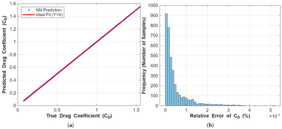
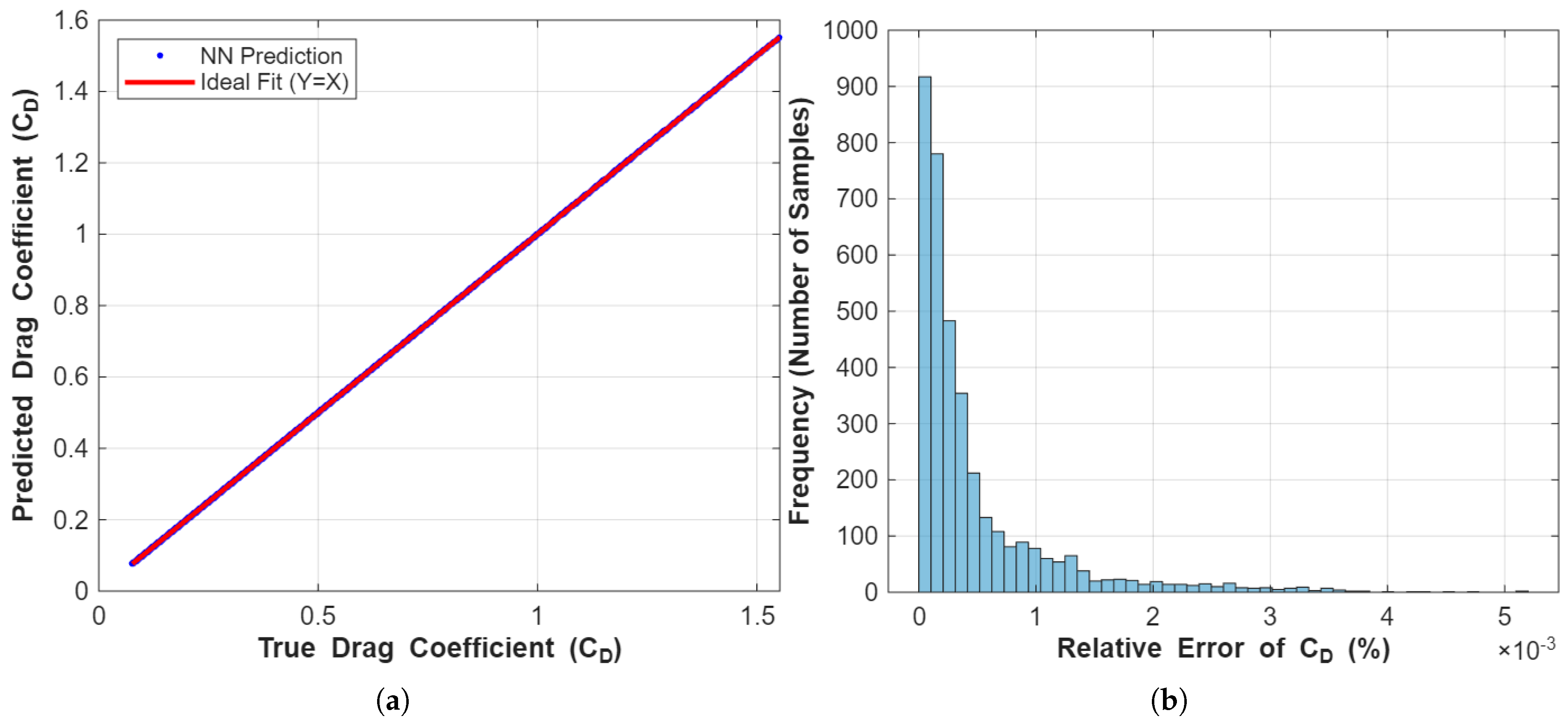
To visually validate the accuracy of the neural network surrogate model, its prediction performance on the aerodynamic dataset is evaluated. Figure 2 illustrates the regression fit and the relative error distribution of the predicted drag coefficient ($C_D$). As shown in Figure 2a, the network predictions perfectly align with the ideal baseline ($Y=X$), indicating a highly precise mapping. Furthermore, the histogram in Figure 2b demonstrates that the relative prediction errors are heavily concentrated near zero, with the maximum relative error strictly bounded below 0.005%. Beyond the exceptional precision, the implementation of this surrogate model provides a remarkable computational advantage. Traditional aerodynamic table look-up procedures, which require iterative solving to determine angle of attack and drag coefficient, are computationally expensive. By mapping the inputs ($C_L,\mathrm{Ma}$) directly to ($\alpha ,C_D$) via the pre-trained neural network, the computational time for each evaluation is reduced from several milliseconds to mere microseconds—an improvement of over two orders of magnitude. This tremendous boost in computational efficiency is a crucial enabler for the rapid online generation of the TAEM trajectory.

Figure 2. Performance validation of the neural network surrogate model: (a) Regression plot of the predicted $C_D$ versus the true $C_D$ from the aerodynamic database. (b) Histogram of the relative prediction error for $C_D$.

The drag force is then calculated as

$$D=q{S}_{\mathrm{ref}}{f}_D(C_L,V)$$

(26)

At this point, all unknown parameters in the dynamic Equation (18), except the state variables, have been analytically expressed.

4. Longitudinal Trajectory Optimization Using the Gauss Pseudospectral Method

Following the analytical dimensionality reduction and model simplification detailed in Section 3, the originally complex trajectory optimization problem has been transformed into an optimal control problem characterized by a low state dimension and reduced dynamic nonlinearity. For such problems, the Gauss Pseudospectral Method (GPM) serves as a potent and efficient numerical solution tool. The selection of this method is primarily based on two key advantages: first, its global polynomial approximation property endows it with spectral convergence accuracy [24,25], allowing for high-precision solutions with a relatively small number of discretization nodes; second, it can uniformly transform differential dynamic constraints, path constraints, and terminal constraints into algebraic constraints within a Nonlinear Programming (NLP) framework, demonstrating strong capability in handling multi-constraint problems. Therefore, this paper employs the GPM to solve the simplified longitudinal optimization problem, aiming to achieve a unified balance between computational efficiency and solution accuracy.

4.1. Optimization Model Formulation

This section constructs the optimization model. Since the value of the angle of attack is inherently related to the variable $\omega$, to ensure the continuity of the angle of attack profile, $\omega$ is treated as a state variable, and its derivative with respect to range, $u=d\omega /dS$, is introduced as the control variable. Consequently, the state vector for the optimization model is defined as $\mathbf{x}={[h,V,\gamma ,\omega ]}^T$, and the control variable is u. The corresponding dynamics model is given by

$$\left\{\begin{array}{c}{\displaystyle \frac{\mathrm{d}h}{\mathrm{d}S}}=tan\gamma \hfill \\ {\displaystyle \frac{\mathrm{d}\gamma }{\mathrm{d}S}}=\omega {cos}^2\gamma \hfill \\ {\displaystyle \frac{\mathrm{d}V}{\mathrm{d}S}}=-{\displaystyle \frac{D}{mVcos\gamma }}-{\displaystyle \frac{g}{V}}tan\gamma \hfill \\ {\displaystyle \frac{\mathrm{d}\omega }{\mathrm{d}S}}=u\hfill \end{array}\right.$$

(27)

The path constraints are

$$\left\{\begin{array}{c}q\le q_{max}\hfill \\ \dot{Q}\le {\dot{Q}}_{max}\hfill \\ n\le n_{max}\hfill \end{array}\right.$$

(28)

where q, $\dot{Q}$, and n are the dynamic pressure, heating rate, and load factor of the vehicle, respectively; $q_{max}$, ${\dot{Q}}_{max}$, and $n_{max}$ are their maximum allowable values.

Furthermore, during the flight, the required drag coefficient is derived from the required lift coefficient. If the required lift coefficient falls outside the vehicle’s permissible range, it indicates that the current trajectory exceeds the vehicle’s aerodynamic capability envelope and is therefore infeasible. Consequently, the optimization constraint for the lift coefficient is formulated as

$$C_{L_{min}}\le C_L\le C_{L_{max}}$$

(29)

where $C_{L_{min}}$ and $C_{L_{max}}$ are the minimum and maximum lift coefficients the vehicle can provide.

The terminal constraints are

$$h\left(S_{\mathrm{all}}\right)=h_f,\gamma \left(S_{\mathrm{all}}\right)={\gamma }_f,V\left(S_{\mathrm{all}}\right)=V_f$$

(30)

During the glide of an unpowered TAEM, both the range and terminal velocity of the aircraft are fixed values, and as mentioned earlier, its trajectory is relatively insensitive to flight time. Therefore, the optimization problem is neither solved by maximizing the range or terminal velocity, nor by minimizing the flight time. To minimize control energy and suppress drastic attitude oscillations, the performance index is designed as the integral of the squared virtual control variable u. This physically ensures the smoothness and engineering feasibility of the resulting trajectory:

$$J={\int }_0^{S_{\mathrm{all}}}{u}^2\mathrm{d}S$$

(31)

It is important to note that the total range $S_{\mathrm{all}}$ is a pre-determined fixed constant calculated from the lateral Bézier curve length obtained in Section 3.1. Therefore, this optimization is formulated strictly as a fixed-independent-variable problem. By employing a standard pseudospectral optimization solver to address this problem, the optimal sequences for the control variables u and $\omega$ are obtained. In the online application phase, only the optimized $\omega$ sequence is required to determine the bank angle and angle of attack analytically. The specific procedure is as follows: First, the lateral trajectory is generated based on the initial and terminal states. Then, the bank angle is calculated using (24), followed by the computation of the required lift coefficient via (25). Finally, the required angle of attack $\alpha$ is solved using (26) based on the required lift. This process yields the complete set of actual flight control commands.

4.2. Initialization of the Optimization

Since the trajectory optimization problem has been significantly simplified in the preceding sections, resulting in a drastic reduction in both dimensionality and nonlinearity, the solution’s sensitivity to the initial guess is markedly reduced. Consequently, the initial guesses for the state and control variables can be simply set as follows:

$$\mathbf{X}={[{\mathbf{x}}_0,{\mathbf{x}}_1,\dots ,{\mathbf{x}}_N]}^T,\mathbf{u}={[u_0,u_1,\dots ,u_N]}^T$$

(32)

where

$$\begin{array}{c}{\mathbf{x}}_i=\left[\begin{array}{c}{h}_0-i\left(h_0-h_f\right)/N\\ {\gamma }_0-i\left({\gamma }_0-{\gamma }_f\right)/N\\ V_0-i\left(V_0-V_f\right)/N\\ 0\end{array}\right]\\ u_i=0\end{array}i=0,1,\dots ,N$$

4.3. Algorithm Flow

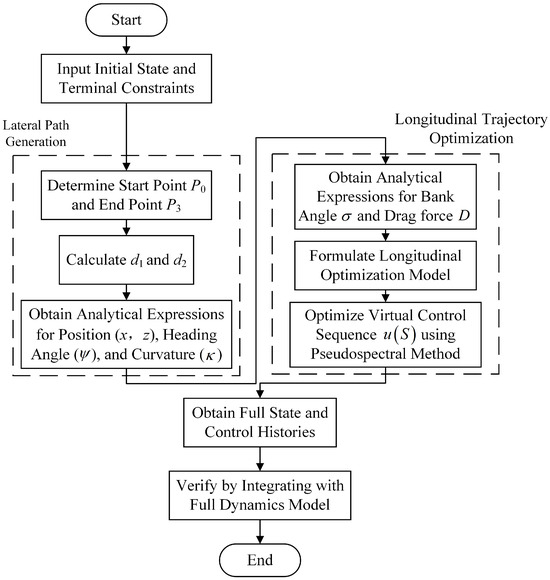
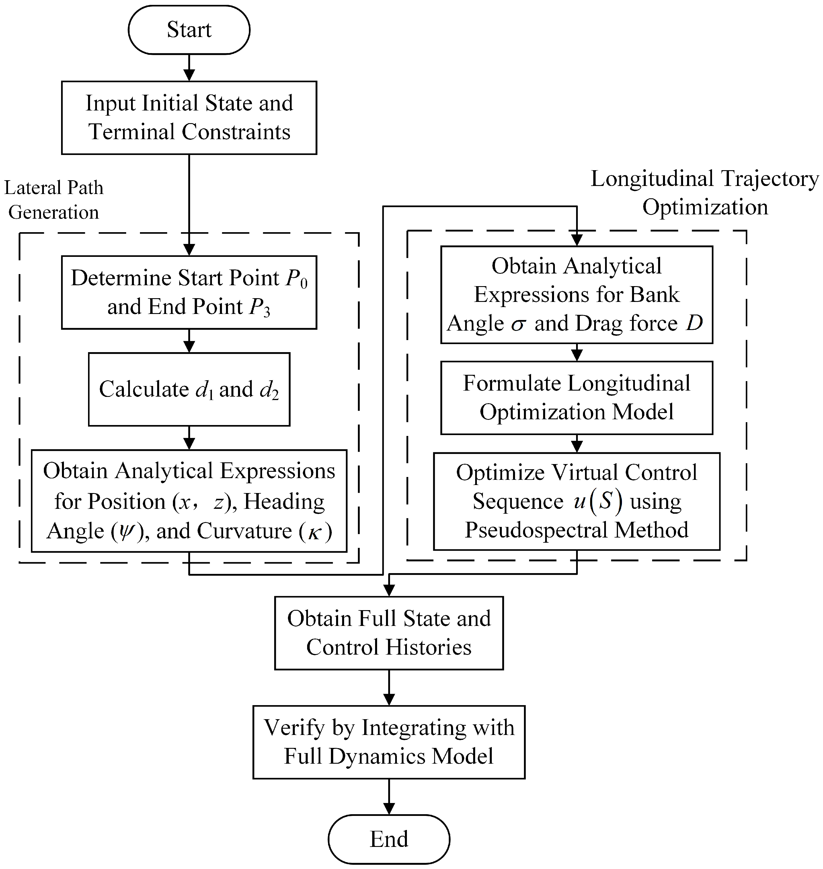
The flowchart of the proposed online trajectory optimization algorithm for the TAEM phase, which is based on analytical lateral planning and dynamic decoupling, is illustrated in Figure 3. The algorithm takes the vehicle’s current real-time state and the mission-specified terminal constraints as inputs. It outputs a complete flight trajectory satisfying all constraints along with the corresponding sequence of control commands. Given its high computational efficiency, this algorithm is designed not merely for a single offline execution but can be executed periodically (e.g., every few seconds) during the flight as a receding horizon update to continuously correct for environmental disturbances. The specific steps are detailed as follows:

Figure 3. Flowchart of the trajectory optimization algorithm.

Step 1:

Analytical Generation of Lateral Trajectory. Based on the initial input and terminal constraints for position and heading, the geometric control points ${\mathbf{P}}_0,{\mathbf{P}}_1,{\mathbf{P}}_2,{\mathbf{P}}_3$ of the cubic Bézier curve are calculated using (6)–(12). Utilizing these control points, analytical expressions for the position $\left(x\right(S),z(S\left)\right)$, heading $\psi \left(S\right)$, and curvature $\kappa \left(S\right)$ with respect to range S are constructed according to (5), (7), and (9).

Step 2:

Rapid Optimization of Longitudinal Trajectory. The curvature function $\kappa \left(S\right)$ obtained in the previous step is substituted into (24) to derive the analytical expression for the bank angle, which is then used in (27) to determine the analytical expression for drag. Based on these derivations, the optimization model described by (28)–(32) is formulated, with initial guesses determined by (34). Subsequently, a standard pseudospectral solver is invoked to rapidly solve this model, generating the optimal virtual control sequence $\omega \left(S\right)$ and the longitudinal state profiles for the current flight condition.

Step 3:

Synthesis of Real Control Commands. The analytical expression for the bank angle and the angle of attack $\alpha$, solved via (25) and (26), are substituted into the full dynamics model (1). The trajectory is then integrated to verify whether the terminal deviations satisfy the accuracy requirements.

5. Numerical Simulation and Analysis

This section presents a comprehensive simulation validation of the proposed TAEM trajectory planning method using the CAV-H vehicle model [26], and the CPU of the computer used for the simulation is Intel i7-11800H (2.30 GHz). The simulation study is organized into three parts. The first part involves trajectory planning under nominal conditions, where the rationality of the planned trajectory is verified by integrating it with the complete dynamics model. The second part consists of Monte Carlo simulations incorporating dispersions in initial positions and states, demonstrating the method’s capability to adapt to deviations propagated from the re-entry phase. The third part conducts a comparative analysis between the proposed method, a profile-based method using a height-dynamic pressure corridor, and the traditional Gauss Pseudospectral Method applied to the complete dynamics model. This comparison aims to substantiate the superiority of the proposed approach in terms of both computational efficiency and solution accuracy.

5.1. Nominal Case Simulation

The initial and terminal states for the vehicle in the nominal case are shown in Table 2.

Table 2. Initial and terminal states of the vehicle.

State	Position (km)	Height (km)	Velocity (m/s)	Flight-Path Angle (deg)	Heading Angle (deg)
Initial State	(95, 120)	27	1500	−2	230
Target State	(10, 0)	4	200	−20	180

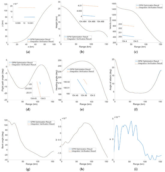
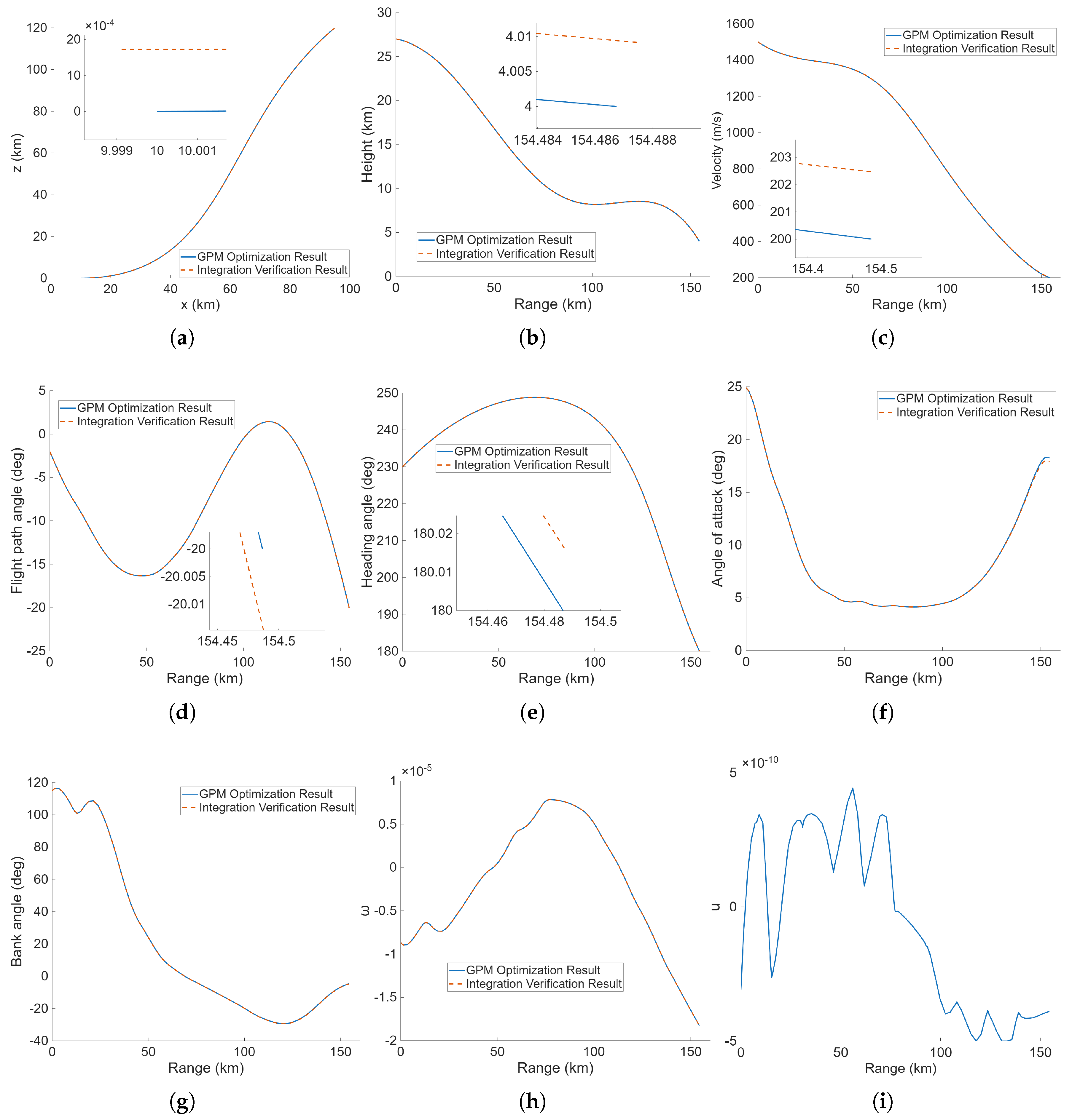
As illustrated in Figure 4, the proposed method successfully generates a reasonable trajectory tailored for the energy management scenario. Throughout the flight, the attitude angles—angle of attack and bank angle—remain smooth and free of abrupt changes, which supports flight stability.

Figure 4. Nominal trajectory simulation diagrams: (a) Ground track. (b) Height vs. range profile. (c) Velocity vs. range profile. (d) Flight path angle vs. range. (e) Heading angle vs. range. (f) Angle of attack vs. range. (g) Bank angle vs. range. (h) $\omega$ vs. range. (i) u vs. range.

The optimized $\omega$ sequence is extracted and applied to the full dynamics model to verify the optimization results via integration. The solution obtained from the GPM (solid line) exhibits a high degree of overlap with the true trajectory obtained by integrating the full dynamics model (dashed line), indicating that the simplified model and the optimization method possess high fidelity. The terminal errors from the integration verification are as follows: height error of 9.13 m, velocity error of 2.46 m/s, flight path angle error of 0.015°, heading angle error of 0.016°, and position error of 1.7 m. The computation time is 0.15 s. The small terminal errors and high computational efficiency demonstrate that the proposed method fully meets the design requirements for TAEM trajectory planning.

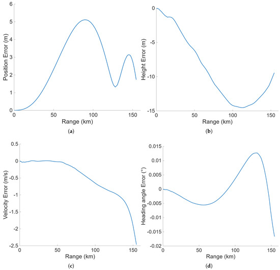
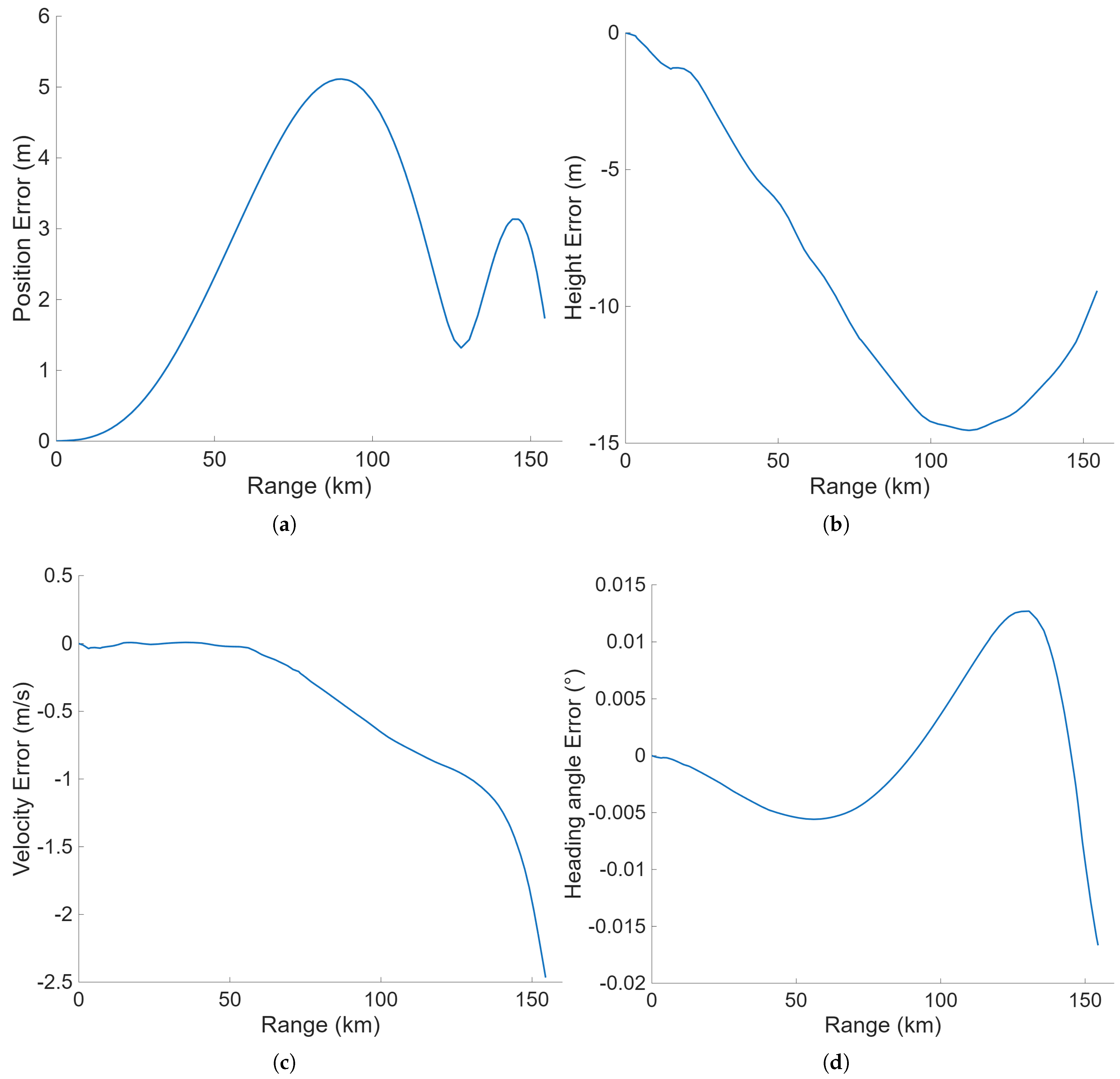
To further illustrate the trajectory tracking accuracy throughout the entire flight, Figure 5 presents the continuous state error profiles (differences between the integration results of the full dynamics and the optimized profiles). As shown, the tracking errors for Position, height, velocity, and heading angle remain tightly bounded at a minimal level across the entire range. This confirms that the dynamically decoupled model maintains exceptionally high fidelity dynamically.

Figure 5. Flowchart of the trajectory optimization algorithm: (a) Position error. (b) Height error. (c) Velocity error. (d) Heading angle error.

5.2. Monte Carlo Targeting Simulation Under Initial State Deviations

When an RLV enters the TAEM phase, its state is subject to significant deviations due to the accumulation of navigation errors, atmospheric model uncertainties, and aerodynamic parameter dispersions during the preceding re-entry phase. To comprehensively and systematically evaluate the reliability and performance consistency of the proposed online planning algorithm in an environment approximating real flight conditions, this section designs a Monte Carlo simulation experiment covering a wide range of initial state dispersions. Referencing the design specifications of the NASA Space Shuttle [7] and related research [27,28], a $3\sigma$ initial state deviation model is constructed as shown in Table 3. This model represents a typical re-entry terminal dispersion footprint and holds practical engineering significance. The experiment generated a total of 2000 random initial state points following a Gaussian distribution, aiming to statistically evaluate the algorithm’s convergence, computational efficiency, and trajectory accuracy.

Table 3. Range of initial state deviation.

State Variable	Mean	$3\mathit{\sigma }$ Value
Initial Height (km)	27	4.5
Initial Velocity (m/s)	1500	600
Initial Flight Path Angle (deg)	−2	3

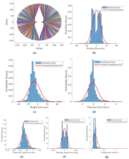
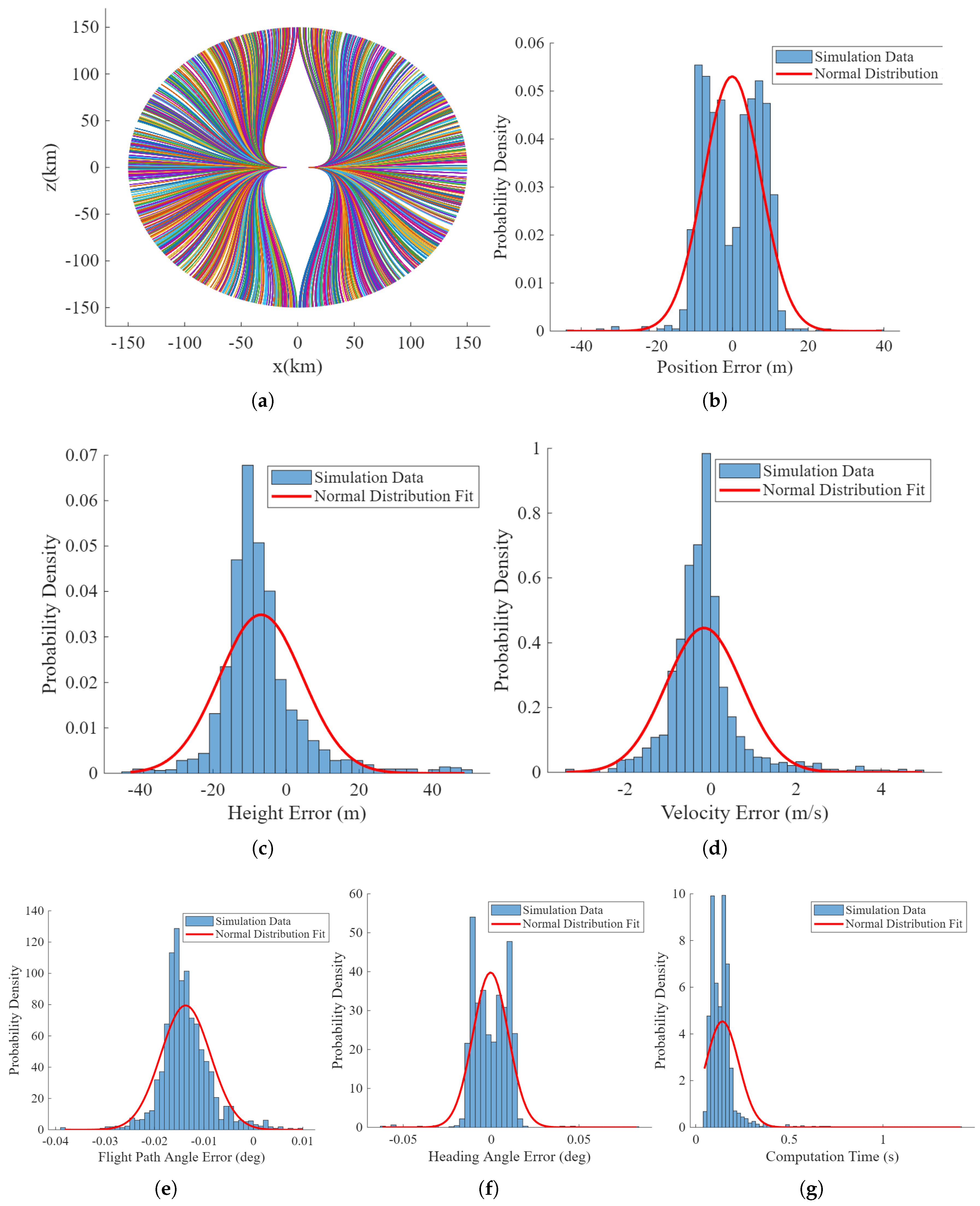
In the 2000 Monte Carlo targeting simulations, the proposed algorithm successfully converged in 1996 cases, achieving a convergence rate of 99.8%, which demonstrates its excellent reliability under complex initial conditions. Figure 6 presents the results of the targeting simulation. Figure 6a shows the ground tracks for all cases, where the vehicle’s starting points are uniformly distributed on a circle with a radius of 150 km centered at the airport, and the vehicles ultimately reach the airport runway from either a positive or negative direction based on their initial positions. Figure 6b–f display the error distribution histograms for the terminal states (position, height, velocity, flight path angle, and heading angle) of the successful simulation cases. Table 4 summarizes the mean, standard deviation, and other statistics of these terminal state errors. The mean values of all terminal state errors are close to zero, and the $3\sigma$ error ranges are extremely small (e.g., position error of 22.56 m and velocity error of 2.69 m/s). These results indicate that the terminal precision achieved by the proposed method is well within the acceptable tolerances for the subsequent approach and landing phase, validating its high accuracy.

Figure 6. Performance statistics from Monte Carlo simulation: (a) Ground track. (b) Terminal position error distribution. (c) Terminal height error distribution. (d) Terminal velocity error distribution. (e) Terminal flight path angle error distribution. (f) Terminal heading angle error distribution. (g) Computation time distribution.

Table 4. Statistical results of terminal state errors.

State Variable	Mean	Standard Deviation ($\mathit{\sigma }$)	$3\mathit{\sigma }$ Value	Max Error
Terminal Height Error (m)	−6.86	11.44	34.31	48.86
Terminal Velocity Error (m/s)	−0.15	0.9	2.69	4.97
Terminal Position Error (m)	−0.1	7.52	22.56	43.75
Terminal Flight Path Angle Error (deg)	−0.014	0.005	0.15	0.038
Terminal Heading Angle Error (deg)	−2.9 × 10−4	0.01	0.03	0.082
Absolute Computation Time per Run (s)	0.14	0.08	0.26	1.41

The computational efficiency of the algorithm is a key metric for assessing its potential for online application. Figure 6g illustrates the distribution histogram of the computation times for the 2000 simulation runs. As can be observed from the figure, the computation times are highly concentrated and do not exhibit significant dispersion or long-tail phenomena, despite the large variations in initial states. It should be noted that the computation time reported here represents the absolute, true execution time for a single complete optimization run, rather than a relative difference between methods.

5.3. Comparative Simulation

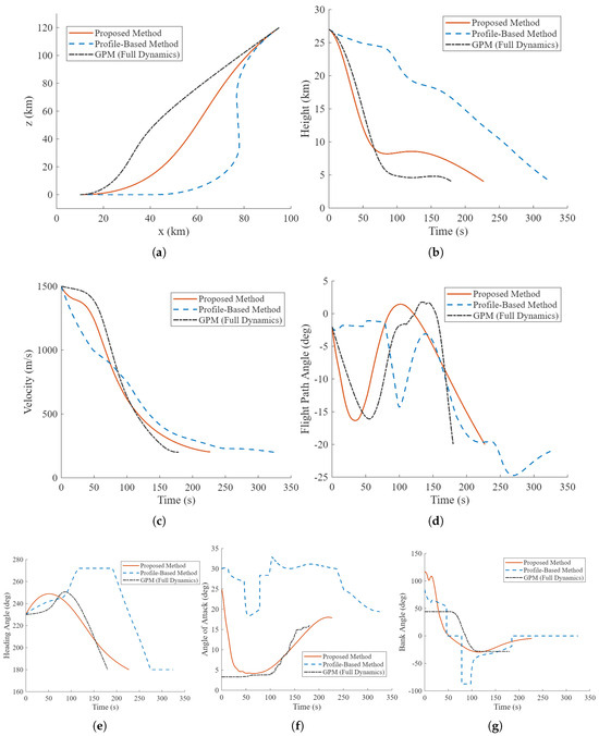
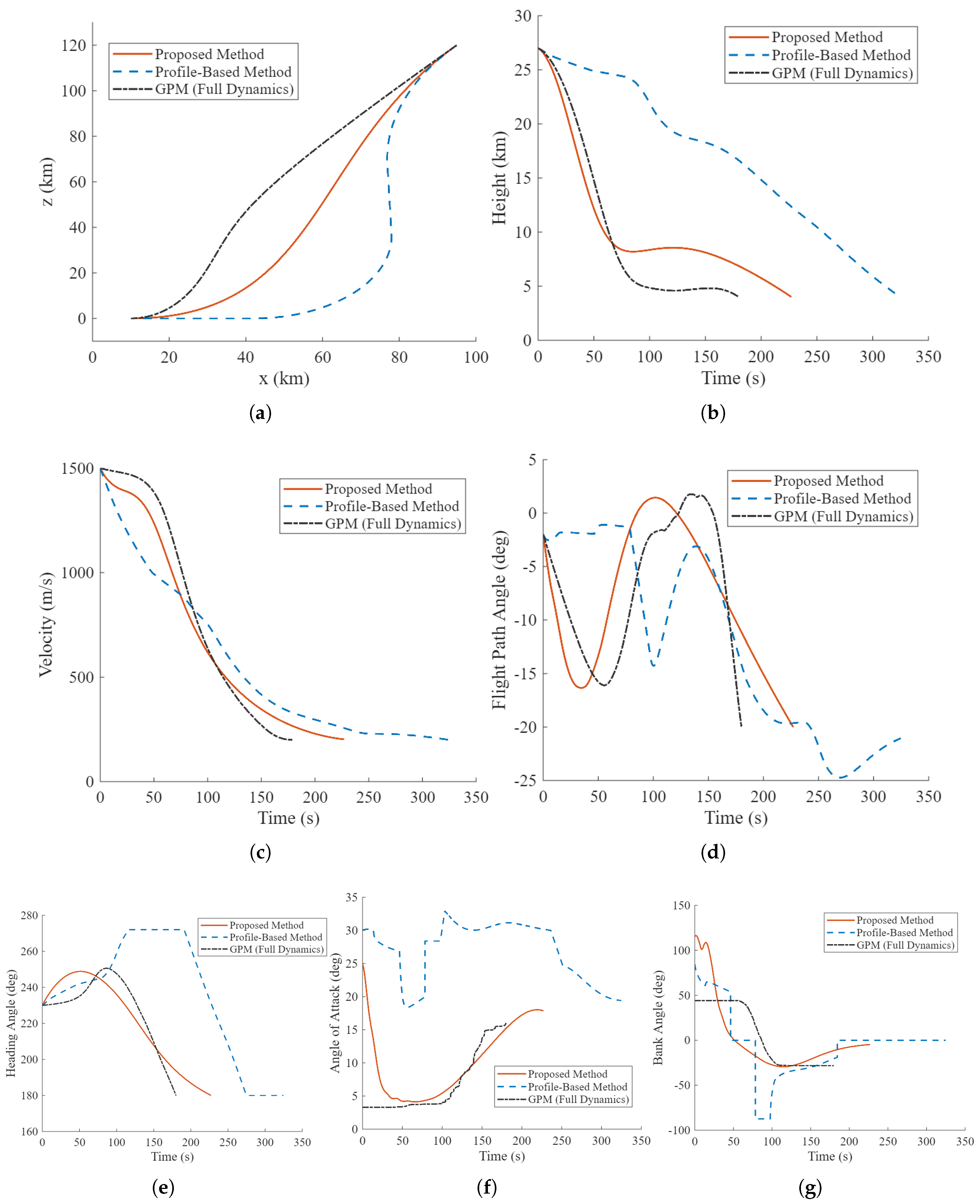
This section conducts a comparative simulation study to demonstrate the advancement of the proposed method by benchmarking it against a profile-based planning method (which utilizes a height-dynamic pressure corridor) and the traditional Gauss Pseudospectral Method applied to the complete dynamics model. The simulation conditions are identical to those used in the nominal case simulation. To ensure a fair and transparent comparison, both the proposed method and the traditional Full Dynamics GPM employed the same number of discretization nodes, and the results are presented as Figure 7 and Table 5.

Figure 7. Simulation diagrams for method comparison: (a) Ground track. (b) Height vs. time. (c) Velocity vs. time. (d) Flight path angle vs. time. (e) Heading angle vs. time. (f) Angle of attack vs. time. (g) Bank angle vs. time.

Table 5. Terminal errors of different methods.

	Proposed Method	Profile-Based Method	GPM (Full Dynamics)
Terminal Position Error (m)	1.97	12.35	1.3
Terminal Height Error (m)	9.13	2.3	−1.93
Terminal Velocity Error (m/s)	2.46	0.24	−0.011
Terminal Flight Path Angle Error (deg)	−0.015	−1.05	0.006
Terminal Heading Angle Error (deg)	−0.016	0.02	−0.013
Absolute Computation Time per Run (s)	0.15	1.21	4.53

From the simulation results presented above, it is evident that the profile-based planning method exhibits a significant terminal flight path angle error. This is attributed to the method’s inherent limitation in constraining the terminal flight path angle. Furthermore, since the planning process requires iterative tuning of design parameters, the computation time remains relatively long. The iteration process is also highly sensitive to the initial guess, leading to poor convergence robustness.

On the other hand, the GPM based on the full dynamics model, while capable of obtaining a high-precision optimal solution, suffers from a computation time as high as 4.53 s. Directly solving the original strongly coupled, nonlinear model results in an extremely complex solution space for the optimization problem. Starting from a simple linear initial guess, the solver requires a large number of iterations to find a feasible solution and may even fail to converge. This makes it ill-suited for online planning tasks.

In contrast, the method proposed in this paper achieves a significant reduction in computation time compared to both the profile-based method and the traditional GPM, while maintaining high terminal accuracy. These characteristics demonstrate its great potential for online applications.

6. Conclusions

This paper proposes a novel online trajectory optimization method for the RLV TAEM phase, integrating analytical lateral planning with equivalent dynamic decoupling. By parameterizing the lateral path with a cubic Bézier curve and introducing a virtual control variable, the complex six-degree-of-freedom problem is rigorously reduced to a simplified longitudinal optimization model, which is then efficiently solved using the Gauss Pseudospectral Method. Simulation results validate that the proposed method achieves stable convergence with simple linear initialization and generates feasible trajectories within 0.26 s ($3\sigma$). The approach demonstrates superior computational efficiency and robustness compared to traditional profile-based and full-dynamics optimization methods, satisfying stringent terminal constraints with high precision. The core concept of “analytical decoupling” provides a robust solution for real-time trajectory planning under strong nonlinearities. While the current algorithm achieves a 0.15 s computation time on a standard desktop CPU, evaluating its performance on space-qualified On-Board Computers (OBCs) is critical. Although OBCs possess lower clock speeds, the current evaluation was conducted in a high-level prototyping environment. By translating the algorithm into highly optimized, compiled languages (e.g., C/C++) standard for flight software, the execution speed will be significantly accelerated. This software-level optimization is expected to fully offset the hardware limitations, ensuring that the trajectory generation can be reliably completed in sub-second times (<1 s) on actual flight processors. Future work will extend this framework by integrating it into a closed-loop simulation (control-in-the-loop Monte Carlo) with an active attitude control system, further verifying its robustness under complex atmospheric disturbances and no-fly zone constraints.

References

- Hanson, J. A plan for advanced guidance and control technology for 2nd generation reusable launch vehicles. In Proceedings of the AIAA Guidance, Navigation, and Control Conference and Exhibit, Monterey, CA, USA, 5–8 August 2002. [Google Scholar]
- National Research Council. Reusable Launch Vehicle: Technology Development and Test Program; The National Academies Press: Washington, DC, USA, 1995.
- Freeman, D.C.; Talay, T.A.; Austin, R.E. Reusable launch vehicle technology program. Acta Astronaut. 1997, 41, 777–790. [Google Scholar] [CrossRef]
- Musk, E. Making humans a multi-planetary species. New Space 2017, 5, 46–61. [Google Scholar] [CrossRef]
- Tewari, A. Atmospheric and Space Flight Dynamics; Birkhäuser: Boston, MA, USA, 2007. [Google Scholar]
- Horneman, K.; Kluever, C. Terminal area energy management trajectory planning for an unpowered reusable launch vehicle. In Proceedings of the AIAA Atmospheric Flight Mechanics Conference and Exhibit, Providence, RI, USA, 16–19 August 2004. [Google Scholar]
- Moore, T.E. Space Shuttle Entry Terminal Area Energy Management; NASA Technical Memorandum NASA-TM-104744; NASA Lyndon B. Johnson Space Center: Houston, TX, USA, 1991.
- Kluever, C.A. Terminal guidance for an unpowered reusable launch vehicle with bank constraints. J. Guid. Control. Dyn. 2007, 30, 162–168. [Google Scholar] [CrossRef]
- Kluever, C.; Horneman, K.; Schierman, J. Rapid terminal-trajectory planner for an unpowered reusable launch vehicle. In Proceedings of the AIAA Guidance, Navigation, and Control Conference, Chicago, IL, USA, 10–13 August 2009. [Google Scholar]
- De Ridder, S.; Mooij, E. Terminal area trajectory planning using the energy-tube concept for reusable launch vehicles. Acta Astronaut. 2011, 68, 915–930. [Google Scholar] [CrossRef]
- Liang, Z.; Li, Q.; Ren, Z. Onboard planning of constrained longitudinal trajectory for reusable launch vehicles in terminal area. Adv. Space Res. 2016, 57, 742–753. [Google Scholar] [CrossRef]
- Kluever, C.A. Simple analytical terminal area guidance for an unpowered reusable launch vehicle. J. Guid. Control. Dyn. 2022, 45, 740–747. [Google Scholar] [CrossRef]
- Lan, X.-J.; Liu, L.; Wang, Y.-J. Online trajectory planning and guidance for reusable launch vehicles in the terminal area. Acta Astronaut. 2016, 118, 237–245. [Google Scholar] [CrossRef]
- Mu, L.; Xie, G.; Yu, X.; Wang, B.; Zhang, Y. Robust guidance for a reusable launch vehicle in terminal phase. IEEE Trans. Aerosp. Electron. Syst. 2022, 58, 1996–2011. [Google Scholar] [CrossRef]
- Mu, L.; Yu, X.; Zhang, Y.M.; Li, P.; Wang, X. Onboard guidance system design for reusable launch vehicles in the terminal area energy management phase. Acta Astronaut. 2018, 143, 62–75. [Google Scholar] [CrossRef]
- Mao, X.; Yu, B.; Shi, Y.; Li, R. Real-time online trajectory planning and guidance for terminal area energy management of unmanned aerial vehicle. J. Ind. Manag. Optim. 2023, 19, 1945–1962. [Google Scholar] [CrossRef]
- Wang, J.; Shao, Y.; Chen, C.; Wang, Z. The design of the flight corridor for the terminal area energy management phase of gliding hypersonic unmanned aerial vehicles. Symmetry 2025, 17, 72. [Google Scholar] [CrossRef]
- Dong, Q.; Zhang, C. Trajectory optimization for RLV in TAEM phase using adaptive Gauss pseudospectral method. Sci. China Inf. Sci. 2018, 62, 10206. [Google Scholar] [CrossRef]
- Poustini, M.J.; Esmaelzadeh, R.; Adami, A. A new approach to trajectory optimization based on direct transcription and differential flatness. Acta Astronaut. 2015, 107, 1–13. [Google Scholar] [CrossRef]
- Wei, Z.; Cheng, Y.; Guo, X.; Liu, S. Hybrid trajectory optimization method and tracking guidance for variable-sweep missiles. Math. Probl. Eng. 2021, 2021, 6669618. [Google Scholar] [CrossRef]
- Mukundan, V.; Maity, A.; Kumar, S.R.; Rajeev, U.P. Terminal phase descent trajectory optimization of reusable launch vehicle. IFAC-PapersOnLine 2022, 55, 37–42. [Google Scholar] [CrossRef]
- Mu, L.; Cao, S.; Wang, B.; Zhang, Y.; Feng, N.; Li, X. Pseudospectral-based rapid trajectory planning and feedforward linearization guidance. Drones 2024, 8, 371. [Google Scholar] [CrossRef]
- Wei, C.; Zhang, Y.; Pu, J.; Zhang, F. Online entry trajectory planning with simultaneous constraints on terminal full-states, flight time and no-fly zones. Aerosp. Sci. Technol. 2026, 168, 111019. [Google Scholar] [CrossRef]
- Fahroo, F.; Ross, I.M. Direct trajectory optimization by a Chebyshev pseudospectral method. In Proceedings of the 2000 American Control Conference, Chicago, IL, USA, 28–30 June 2000; pp. 3860–3864. [Google Scholar]
- Garg, D.; Patterson, M.; Hager, W.W.; Rao, A.V.; Benson, D.A.; Huntington, G.T. A unified framework for the numerical solution of optimal control problems using pseudospectral methods. Automatica 2010, 46, 1843–1851. [Google Scholar] [CrossRef]
- Phillips, T.H. A Common Aero Vehicle (CAV) Model, Description, and Employment Guide; Schafer Corp. for Air Force Research Laboratory and Air Force Space Command: Arlington, VA, USA, 2003. [Google Scholar]
- Shen, Z.; Lu, P. Onboard generation of three-dimensional constrained entry trajectories. J. Guid. Control. Dyn. 2003, 26, 111–121. [Google Scholar] [CrossRef]
- Hu, Y.; Gao, C.; Li, J.; Jing, W.; Chen, W. A novel adaptive lateral reentry guidance algorithm with complex distributed no-fly zones constraints. Chin. J. Aeronaut. 2022, 35, 128–143. [Google Scholar] [CrossRef]
Disclaimer/Publisher’s Note: The statements, opinions and data contained in all publications are solely those of the individual author(s) and contributor(s) and not of MDPI and/or the editor(s). MDPI and/or the editor(s) disclaim responsibility for any injury to people or property resulting from any ideas, methods, instructions or products referred to in the content. |
© 2026 by the authors. Licensee MDPI, Basel, Switzerland. This article is an open access article distributed under the terms and conditions of the Creative Commons Attribution (CC BY) license.