


Abstract
The strategy developed to carry out a scaled test program aimed at reproducing the behavior of skin heat exchangers to alleviate the heat dissipation requirements in future hybrid electric propulsion regional aircrafts is presented. The test program is intended to reproduce the dimensionless thermal response characterizing the skin heat exchanger on a predefined nominal cruise flight operation, while conducting the tests in a wind tunnel operating at low velocities and near-standard atmospheric conditions. For that purpose, dimensional analysis is used to define the geometrical scale and approach flow conditions in the wind tunnel test program, so that the dimensionless parameters describing the skin heat exchanger thermal response resemble the ones taking place under nominal flight conditions. The validation of the scaling strategy is achieved by comparing dimensionless parameters characterizing the turbulent momentum and heat transfer processes taking place at the skin heat exchanger/airflow interface surface in the flight and wind tunnel environments, by using CFD analysis based on two-equation and SST RANS turbulence modeling. The comparison reveals that the adopted wind tunnel strategy is indeed capable of closely reproducing the heat transfer process taking place in the flight environment, thus paving the way to achieve mid TLR validation of the skin heat exchanger technology.
1. Introduction
Regional aircrafts based on hybrid electric propulsion (HERA) are one of the key elements to reduce carbon emissions in the short and medium range aircraft operation, having in mind the ambitious objective set in the Strategic Research and Innovation Agenda (SRIA) [1], which entails a 50% emission reduction in Green House Gas (GHG) with respect to current state of the art technology for HERA. Conceptual studies indicate that hybrid electric propulsion leads to heavier aircrafts than the thermal ones, and HERA only makes sense in a scenario of cutting CO2 emissions [2]. Different ongoing HERA projects are already being developed, aiming at having platform airworthiness by the late-2020s for small 20 seats concepts and by the mid-2030s for 50–100 seats and distances less than 500 km. For this latter application, HERA should include hybrid electric propulsion based on batteries or fuel cells as energy sources, supported by SAF or hydrogen burning for the thermal source, to reach up to 90% lower emissions while being fully compliant with International Civil Aviation Organization (ICAO) noise rules.
To be successful, HERA development will need to integrate and enable disruptive technologies including high voltage MW scale electrical distribution, new hybrid electric propulsion and related new energy storage at low GHG generation, and high-capacity thermal management. Regarding this latter aspect, HERA will have to face very demanding on-board thermal management issues, as heat dissipation requirements in these aircrafts are expected to undergo order of magnitude increases with respect to current needs, typically escalating from levels to close to figures. As a result, advanced compact, lightweight, and highly efficient heat dissipation concepts will need to be developed in order to meet the stringent heat management requirements attached to HERA.
One of the concepts being investigated is the skin heat exchanger (SHX), which uses the skin of the aircraft and the airflow sweeping over it as the heat sink process. To meet the high heat dissipation capacity and compact architecture demanded by highly efficient HERA designs, SHX systems will need to incorporate phase change in the aircraft bound cooling circuit. Reviews of conceptual designs for thermal management in HERA [3,4] indicate that SHX combined with a gas/liquid cooling circuit including phase change could offer significant benefits, minimizing drag penalties induced by alternative ram air driven heat exchangers. Furthermore, conceptual design studies point out that ram air could not address alone the high-demanding heat dissipation required by HERA without incurring unacceptable penalties on aircraft aerodynamics [5,6]. However, in order to complement or to be a meaningful alternative to conventional heat drain concepts, SHX technology must demonstrate high enough heat exchange fluxes to offset its weight and size penalties.
A potential hurdle for the integration of SHX technology in HERA could be the introduction of composite materials in aircraft structures [7], which have proved to reduce fuel consumption by 12% in the last generation of aircrafts but which could limit efficient heat transfer from the aircraft skin [3], though additive manufacturing with metals [7] or aluminum skin could offer a good trade-off solution for SHX heat dissipation surfaces. A more detailed conceptual study on the impact of SHX on aircraft aerodynamics [8] postulates that friction drag decreases on turbulent boundary layers acting as SHX heat sinks, even though the study considered simple heat transfer coefficients based on flat plate correlations [9,10,11,12]. Further assessment of the SHX potential aerodynamic performance on lifting surfaces has been conducted with the help of CFD studies [13,14,15,16] incorporating one and two-equation RANS turbulent models, including Spalart–Allmaras, and SST closures [17,18], where the ability of CFD simulations to track heat transfer and aerodynamic coefficients was validated against experimental data of icing devices on wing profiles [19] with some degree of success. The optimal position of SHX installed on the lifting surfaces seems to be at the pressure side [13,14], where a smaller impact on the aerodynamic performances is expected. However, heating both the suction and pressure sides of the wing [15,16] could degrade aerodynamic efficiency by up to 15% at high surface temperatures [15], due to the negative impact on the suction side of the aerodynamic profiles. Furthermore, heat transfer delivered by SHX could be compromised at low velocities and high power-demanding regimes, such as take-off or climbing [13,14]. These flight regimes could require a temporary back-up heat sink process like one based on the fuel delivery system, or else SHX could take advantage of the high-speed slipstream from the propellers [15]. An alternative to lifting surface installation of SHX is the sponsons surfaces for the landing gear, offering a close to zero pressure gradient (ZPG) environment which could reduce friction drag and allow an efficient installation of the SHX hardware.
Conceptual studies for the selection of the working fluid in the coolant circuit of SHX have placed the focus on the family of HFO coolants [20,21] with change of phase models [21,22], which are categorized as ozone-friendly, low global warming potential. Semi-empirical correlations for heat transfer coefficients on pipes and flat plates have demonstrated that HFO-1234yf and 1233zd exhibit great potential for reducing the size of the SHX surface. With regard to the relative coolant and airflow directions, semi-empirical procedures [21,23] concluded that parallel co-flows demonstrate superior mechanical and heat transfer performances than counter-flow configurations. For the cooling circuit geometries, current advances in additive manufacturing make possible introducing complex designs based on Triply Periodic Minimal Surfaces (TPMS) and wavy or riblet cooling channel topologies [24,25,26]. However, considering the present onboard flight application and that the focus of this study is on establishing the strategy for conducting scaled SHX tests, simple cooling conduits with a square cross section seem to be a good choice for the coolant duct, based on a compromise between optimizing heat transfer and pressure drop coefficients with minimum weight and size penalties [20,21,23,27].
Increasing the SHX TRL level beyond conceptual studies calls for preliminary, dedicated experimental validation programs that can reproduce the main features of the SHX operation in nominal flight operation. Due to the present conceptual stage of HERA aircrafts, very little SHX dedicated experimental data is available in the open literature relevant to this application. An air–air surface heat exchanger for mild heat sink requirements has been experimentally characterized in ground conditions [28], showing its potential as an aerodynamically optimized heat sink to be used for cooling aircraft electronic equipment. Furthermore, a preliminary characterization of an air/liquid SHX concept based on a folded core aircraft skin has been characterized under natural convection heat transfer regime by using temperature sensitive paints and one-dimensional analytical models, concluding that the optimal pitch between consecutive cooling channels is of the order of the channel’s characteristic size [29].
More representative experimental environments require an external to aircraft airflow characterized by Mach numbers with nominal flight pressure and temperature levels. In addition, the boundary layer of the airflow sweeping over the SHX airflow exposed surface should be turbulent with realistic boundary layer scales. Performing the early SHX development tests while matching all these airflow conditions is not feasible using wind tunnels operating at near-standard atmospheric conditions. As a result, it is necessary to develop a test strategy to reproduce the SHX operation to be found in the nominal flight conditions while using near-standard, atmospheric wind tunnel test benches. The aim of this work is to develop such strategy for setting a wind tunnel test environment that would establish close physical similarity with the results achieved by SHX under nominal HERA flight conditions, by using a low-speed wind tunnel operating at near-standard atmospheric conditions as the SHX external airflow generation system.
2. SHX Airflow Modeling
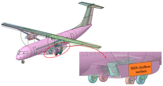
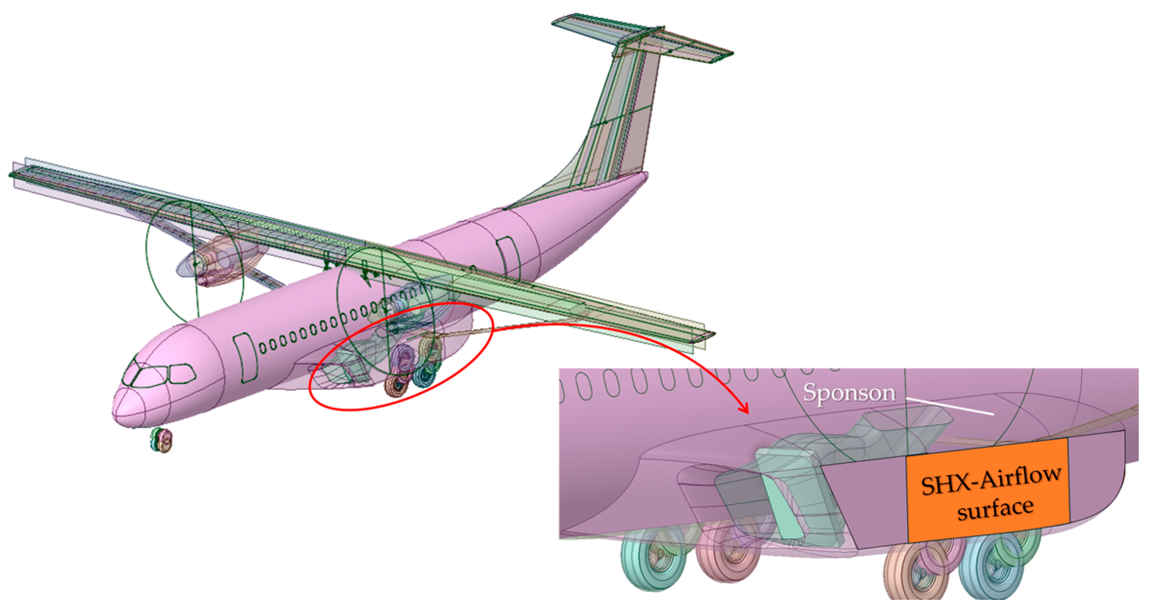
In SHX architectures, either the fuselage or the lifting surfaces can be used as surfaces to dissipate heat to the airflow sweeping the aircraft. For HERA architectures, although lifting surfaces can be considered as potential installation sites, aerodynamic performance issues indicate that the sponsons used as fairing for the aft landing gear could be the optimal choice to base the SHX airflow exposed surfaces [13,14,15]. This option has many advantages, as it allows locating the SHX elements away from the cabin to minimize SHX integration problems while benefiting both from relatively thin yet turbulent boundary layer development to augment the heat transfer coefficient and provide enough surface to achieve heat dissipation levels of the order of . Figure 1 shows the sponson installation zone to locate the airflow exposed SHX surface in a conceptual HERA design. With this arrangement, the expected available SHX heat dissipation area would be of the order of per sponson, and the leading edge of the SHX airflow exposed surface could be located at distances from the sponson leading edge of the order of , thus ensuring a turbulent yet thin boundary layer sweeping over the SHX airflow exposed surface.
Figure 1.
HERA concept and airflow exposed SHX surface using the sponson location as SHX installation site.
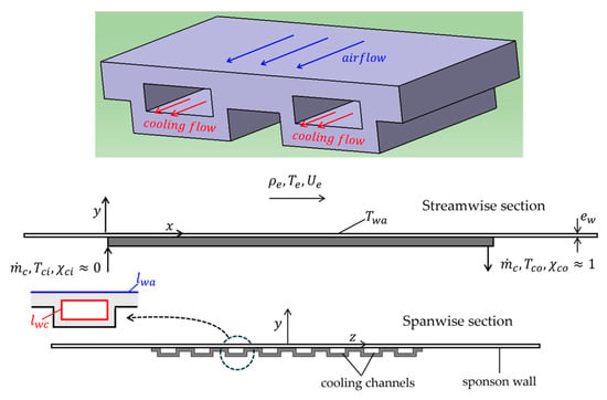
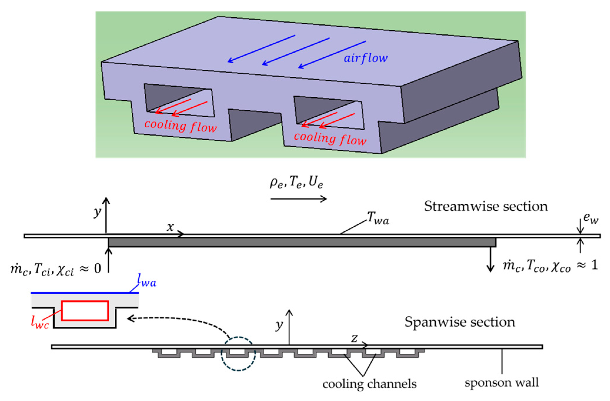
A SHX conceptual basic geometry is shown in Figure 2. The cooling fluid flows over several parallel cooling channels which are also exposed through the sponson wall to the aircraft exterior airflow, with exterior unperturbed properties of density, temperature and velocity respectively given by . This airflow is limited by the sponson wall having temperature . For the schematic design shown in Figure 2, each cooling channel exhibits a rectangular cross section as previous studies [20,21,23,27] indicate that it could offer benefits to maximize the heat transfer from the cooling fluid while ensuring not too large penalties in pressure drop, weight and size. To achieve high heat fluxes and thus a compact layout, the SHX operates the cooling fluid allowing phase change in the cooling channels. Thus, the cooling fluid with mass flow rate enters the SHX cooling channels as a slightly superheated vapor with temperature and liquid mass fraction , and leaves it as a slightly subcooled liquid with temperature and liquid mass fraction . Figure 2 also shows the coordinate system used to describe the SHX/airflow heat transfer, having its origin on the SHX wall exposed to the airflow and at the streamwise location where the leading edge of the SHX is placed, with the axis running parallel to the external airflow streamwise direction and the axis being normal to the SHX wall exposed to the airflow and pointed towards the latter.
Figure 2.
SHX schematic view, showing a segment of the SHX and streamwise and spanwise sections with cooling channel detail.
The sponson wall is represented in Figure 2 as the surface denoted with wall thickness . Each cooling channel has effective heat exchange perimeters in contact with the cooling fluid and with the external airflow respectively denoted as , with . Except for local spanwise end effects, each cooling channel can be considered to operate under periodic spanwise conditions. Table 1 summarizes the main nominal flight operating parameters, with subscripts respectively denoting SHX exterior airflow and cooling channel fluid conditions. These correspond to HERA operating in nominal cruise at ISA flight level FL250 and exterior Mach number , as described in [20]. A nominal design with characteristic distance of between the sponson leading edge and the SHX leading edge is considered to provide space to accommodate the different hardware components included in the SHX system with minimum aerodynamic penalty.
Table 1.
SHX main operating parameters for HERA application at nominal flight conditions [20].
The requirement set in Table 1 for the SHX/airflow dissipated heat flux implies that considering two independent SHX units with characteristic surface each of means a total heat dissipation of at least can be achieved.
2.1. SHX Description Simplification
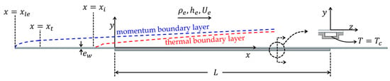
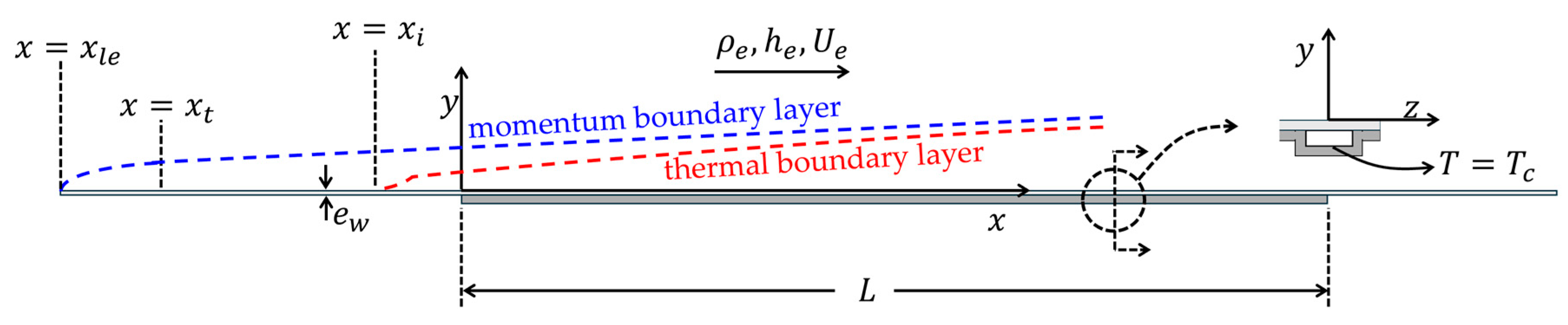
As a result of the phase change, the SHX cooling channel operates almost at isobaric and isothermal conditions. Thus, the temperature in the SHX solid wall in contact with the cooling fluid can be considered to take a uniform value in all its length, corresponding to the cooling fluid condensation temperature at pressure . In addition, the airflow established over the sponson surface can be considered to develop as a zero-pressure gradient (ZPG) turbulent boundary layer, as schematically depicted in Figure 3.
Figure 3.
Airflow momentum boundary layer, shown as broken blue line and thermal boundary layer, shown as broken red line, developing over the sponson and SHX surfaces exposed to the airflow.
The SHX of length L spans the streamwise coordinates . As stated above, a uniform temperature boundary condition can be prescribed at the SHX solid wall limiting the fluid cooling channels. For the solid SHX and sponson walls not exposed to the airflow or to the cooling fluid an adiabatic boundary condition can approximately be considered. The airflow momentum boundary layer will have its origin at the leading edge of the sponson, . Shorty after it, the boundary layer will undergo transition to turbulence at a streamwise location denoted as in Figure 3. As a result of heat conduction taking place through the sponson wall, the airflow thermal boundary layer will be initiated upstream of the SHX, at a location denoted as in Figure 3. Likewise, some heat exchange to the airflow will also take place downstream from the SHX, at locations verifying .
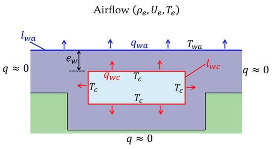
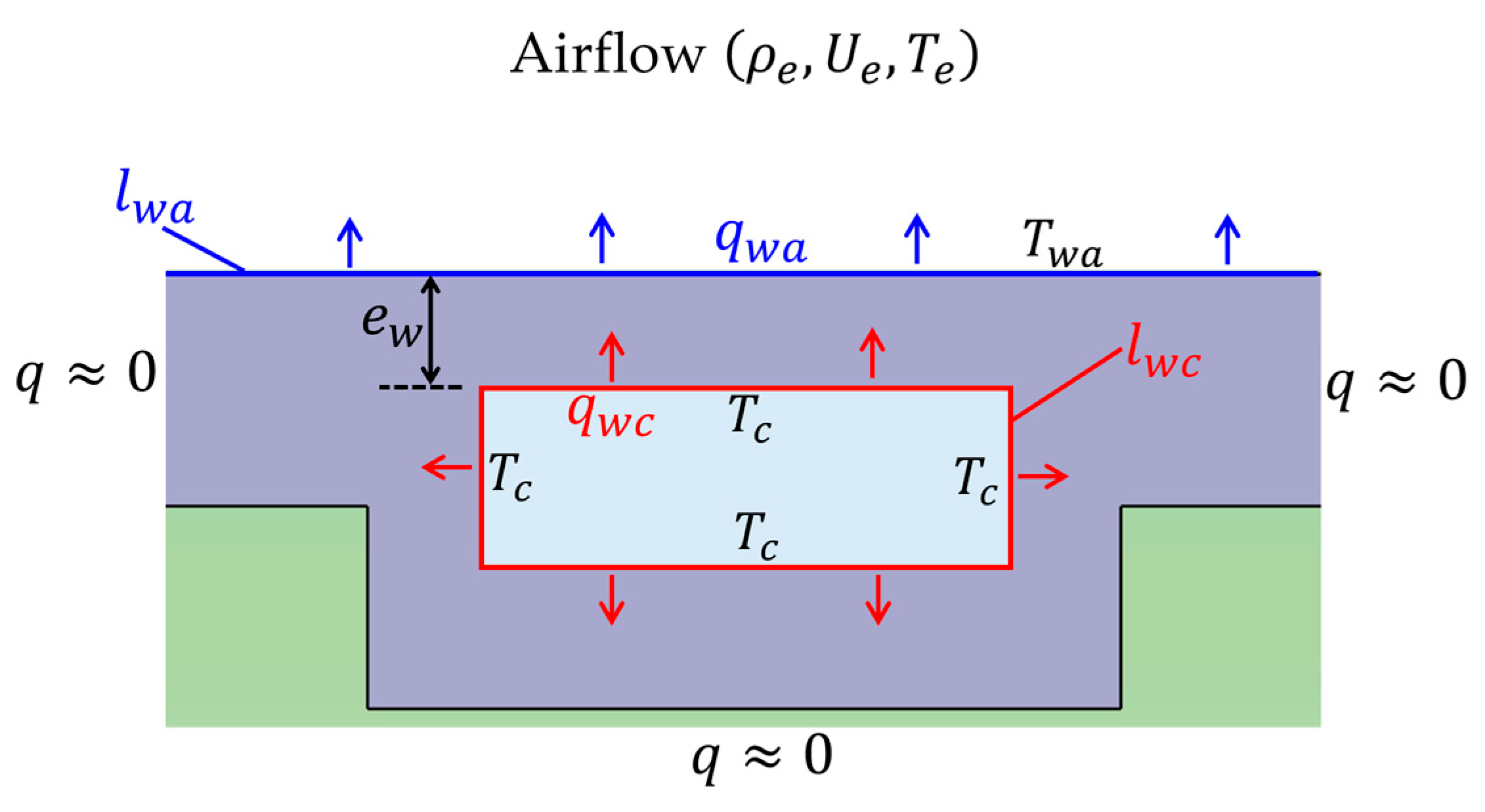
Considering the streamwise segment covered by the SHX, an estimate of the spanwise averaged solid wall temperature exposed to the airflow can be given after establishing the balance between the heat exchanged between the SHX solid wall on both its airflow and cooling fluid interfaces, as schematically depicted in Figure 4. Denoting respectively as the average heat flux in the perimeter of the cooling channel and the spanwise average heat flux at the SHX/airflow wall, and considering the limit , the heat exchanged between the cooling channel and the SHX solid wall is eventually dissipated into the external airflow by the heat exchanged at the SHX solid wall in contact with the airflow. This implies:
with being a characteristic value of the Stanton number for the SHX–airflow heat exchange process, and with denoting the heat conductivity of the solid SHX/sponson wall. Expression (1) can be rearranged to give:
Figure 4.
Schematic representation of the heat flux path in the SHX, showing a cross-stream cut of the SHX subject to cooling fluid and external air flows. Red arrows: cooling fluid to SHX solid wall heat flux. Blue arrows: SHX solid wall to external airflow heat flux.
The estimate given in (2) for the dimensionless parameter follows after considering values presented in Table 1 and SHX solid wall parameters , , .
The first important implication of estimate (2) is that, except for local spanwise end effects, the spanwise modulation of the airflow magnitudes should be weak and thus the airflow boundary layer should be almost two-dimensional. This suggests defining airflow magnitudes that are averaged along the spanwise direction , in a spanwise interval equal to half the spanwise separation between consecutive cooling channels. In what follows it will be assumed that airflow magnitudes have been spanwise averaged in this fashion.
A second important implication of (2) is that, considering values given in Table 1, we can write for the airflow:
with being the temperature difference taking place across the airflow boundary layer, which also heats up from the combined action of compressibility effects and of the reduced velocities taking place near the solid wall. Denoting as the airflow temperate increment due to this effect, and according to the flight operation values given in Table 1, it follows:
Expression (4) indicates that the airflow temperature increase resulting from the flight Mach number and viscous heating is an order of magnitude smaller than the one established by the SHX operation. Thus, the equations describing the development of the airflow boundary layer can be approximated in the first instance by considering the limit , with airflow compressibility effects only showing through the heating of the SHX solid wall by the SHX cooling flow.
2.2. Airflow and SHX Solid Wall Differential Equations Description
For the laminar case and with the momentum and thermal boundary layers sharing the same origin, it is possible to define a change in variables such as the Stewartson transformation [12] that will define an equivalent incompressible boundary layer to account for non-negligible Mach number effects. However, such transformations are based on simplifications taken for the molecular transport terms that cannot be applied to the turbulent boundary layer because of its multiscale character and the difficulty to properly handle the turbulent stresses and energy fluxes. In addition, in the present context, the momentum and thermal boundary layers do not share the same origin. Thus, and having in mind (4), the limit will be considered for the equations governing the mean airflow boundary layer and the solid wall temperature, which in that case can be written as:
In these expressions and respectively denote Favre and time averaged magnitudes, with being the Cartesian velocity components, denoting the airflow density, enthalpy and temperature, and describing the SHX solid wall temperature. In addition, respectively denote the dynamic molecular and turbulent viscosities, whereas represent the molecular and turbulent Prandtl numbers. The thermodynamics closure for the above equations can be expressed as:
The simplified viscosity law introduced in (6) is very accurate for temperatures close to [30]. As viscous effects for the system of Equation (5) are only significant in the turbulent wall layer, characterized by temperatures close to , the simplified viscosity law included in (6) should be very representative.
A turbulent closure for Equation (5b,c) can be proposed by introducing two scales characterizing the development of the turbulent boundary layer, namely the wall friction velocity and its global thickness given by the Rotta–Clauser length scale [31], which are defined as:
With these two scales, a local model for the turbulent viscosity can be proposed [32] to give:
The system (5)–(7) must be complemented with appropriate boundary conditions. If the airflow inlet is defined at a location sufficiently upstream from the SHX, the airflow boundary conditions become:
with denoting the dimensionless velocity profile of the ZPG, adiabatic turbulent boundary layer.
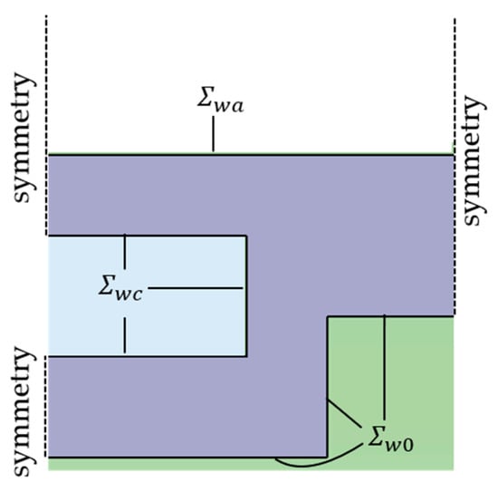
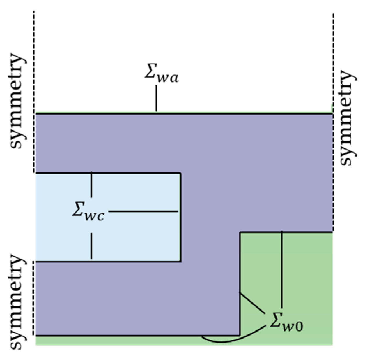
The surfaces defining the boundaries of the SHX solid wall (Figure 5) can be classified as the solid wall–airflow boundary, ; the solid wall–cooling channel boundary, ; and the solid wall not in contact with either the external airflow or the cooling fluid, . If the geometry of the cooling fluid channel and the inter-channel separation are of the order of the sponson wall thickness , surfaces introduce two characteristic lengths: the SHX streamwise length , and the sponson wall thickness . Boundary conditions at the solid wall boundary not in contact with the airflow can then be specified as:
Figure 5.
Schematic view of surfaces defining the boundaries of the SHX solid wall.
In addition, the compatibility of temperature and heat flux must be imposed at the solid wall/airflow interface surface :
Upstream and downstream of the SHX, Equation (5d) can be integrated along the directions to give a one-dimensional equation for the streamwise evolution of the cross-stream averaged sponson wall temperature :
with again representing a characteristic value of the Stanton number for the SHX/airflow heat transfer. Equation (9) defines a characteristic length that sets the scale for the length upstream and downstream from the SHX where the cross-stream averaged sponson wall temperature relaxes to the value imposed by the external flow:
At streamwise locations the sponson wall temperature should approach the exterior airflow temperature. Thus, this location can be selected to specify, using expressions (8c), the state of the adiabatic, ZPG turbulent boundary layer approaching the SHX. Considering , it results in:
2.3. Dimensional Analysis and Dimensionless Formulation
Dimensional analysis of the system (5)–(7) with boundary conditions (8) and definition (11) allows the writing of the following generic dependence for the unknowns:
The dimensionless formulation of the airflow/SHX solid wall problem can be achieved by selecting an appropriate set of parameters. Specifically, exterior airflow magnitudes and the boundary layer thickness at can be used for that purpose:
Using these magnitudes as the set to render a dimensionless expression of the airflow/SHX solid wall problem, leads to the definition of the following dimensionless variables:
The additional dimensional parameters that appear in (12) generate a number of controlling dimensionless parameters. Specifically:
The parameter appears when writing the dimensionless expression of the temperature and heat flux continuity condition (8f) at the sponson wall/airflow interface surface:
The dimensionless parameters that appear in (15a,b) have been classified according to their impact in the dimensionless formulation of the airflow/SHX solid wall heat transfer process. Thus, parameters and control the development of the airflow boundary layer and thus they should be carefully matched in a scaled test program. Assuming that the exterior airflow conditions are given, matching these two parameters sets the appropriate scale for the thickness of the boundary layer approaching the SHX. In turn, this value determines the geometrical scale of the wind tunnel tests, including the characteristic thickness setting the sponson and SHX solid walls.
Matching the parameters that appear in (15b) is less critical. In particular, the parameter is just the ratio between the thermal conductivities of the SHX solid wall and of the airflow at temperature . For the value of this temperature given in Table 1 and it follows . This very large order of magnitude ensures that the parameter that appears in expression (2) remains small and that the temperature of the airflow/SHX solid wall interface surface becomes close to . Thus, as long as the specific value adopted by should have a secondary effect in the airflow/SHX heat transfer process, only leading to small deviations in the dimensionless temperature and heat flux values for the airflow solution. Small discrepancies of will also have a secondary impact in the specific value of the location where to specify the initial conditions for the approaching turbulent boundary layer, as its impact is somewhat smoothed by the presence of the root square in definition (15b).
Regarding the specification of the initial state for the airflow boundary layer at , recall that the streamwise position is defined as the location where the laminar to turbulent transition takes place over the sponson wall. Furthermore, since over the streamwise segment the turbulent boundary layer develops under adiabatic equilibrium conditions, it can be written as:
Considering the above discussion, the dimensionless dependence of the airflow and of the SHX solid wall temperature can be written as:
The dimensionless friction velocity, boundary layer thickness, and turbulent viscosity become:
Expression (18) give the dependence of the dimensionless airflow magnitudes and solid wall temperature, which allows proposing the appropriate scaling of wind tunnel tests conducted at near-standard atmospheric conditions to reproduce the heat transfer process taking place over the sponson wall in nominal flight operation. Considering that the parameters are independent of the airflow operation conditions, the following constraints should be enforced to ensure physical similarity of the airflow/SHX heat transfer process between the wind tunnel scale tests and the nominal flight operation:
- Geometrical similarity
- Identical values of key dimensionless parameters, namely, .
- Large enough value of the dimensionless parameter , .
With the conditions given in Table 1, only the initial value of the boundary layer thickness needs to be specified at streamwise location to fully define the magnitude set given in (13) for the nominal flight operation. The evolution of the boundary layer upstream of the SHX can be estimated by considering a characteristic distance separating the leading edges of the sponson and of the SHX, and that the sponson wall behaves as a flat plate. Selecting as a safe margin to install the SHX with minimum aerodynamic penalty, the evolution of the boundary layer over the sponson wall would include first a short laminar development followed by a transition process and a posterior turbulent development. The transition Reynolds number based on the distance from the sponson leading edge will depend on the free stream turbulence level and on the sponson’s leading edge region geometry. Considering a characteristic transition Reynolds number based on the exterior airflow properties and on development distance of the order of [12], the location of transition for nominal flight operation verifies:
The evolution of the ZPG sponson boundary layer after transition can be estimated by considering the logarithmic friction law and von Karman’s boundary layer equation [33]:
Rearranging these equations gives the evolution of the Reynolds number defined by the exterior airflow properties and development distance as a function of a Reynolds number constructed from the product :
The lower bound for the integral in (22) can be taken with a characteristic value at transition , although for development distances verifying any value of this Reynolds number selected in the range will have negligible impact in the evolution of expression (22). Equations (21a) and (22) then give the evolution of the two scales characterizing the turbulent boundary layer that develops over the sponson wall upstream of the SHX. These equations can be applied to determine these two scales at station given in (11). For the nominal flight conditions, considering a sponson wall made of aluminum alloy with it results in:
Solving Equations (21a) and (22) for leads to establishing the scales of the turbulent boundary layer at for the nominal flight operation:
3. Wind Tunnel Scaled Test Specification
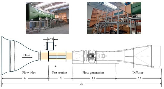
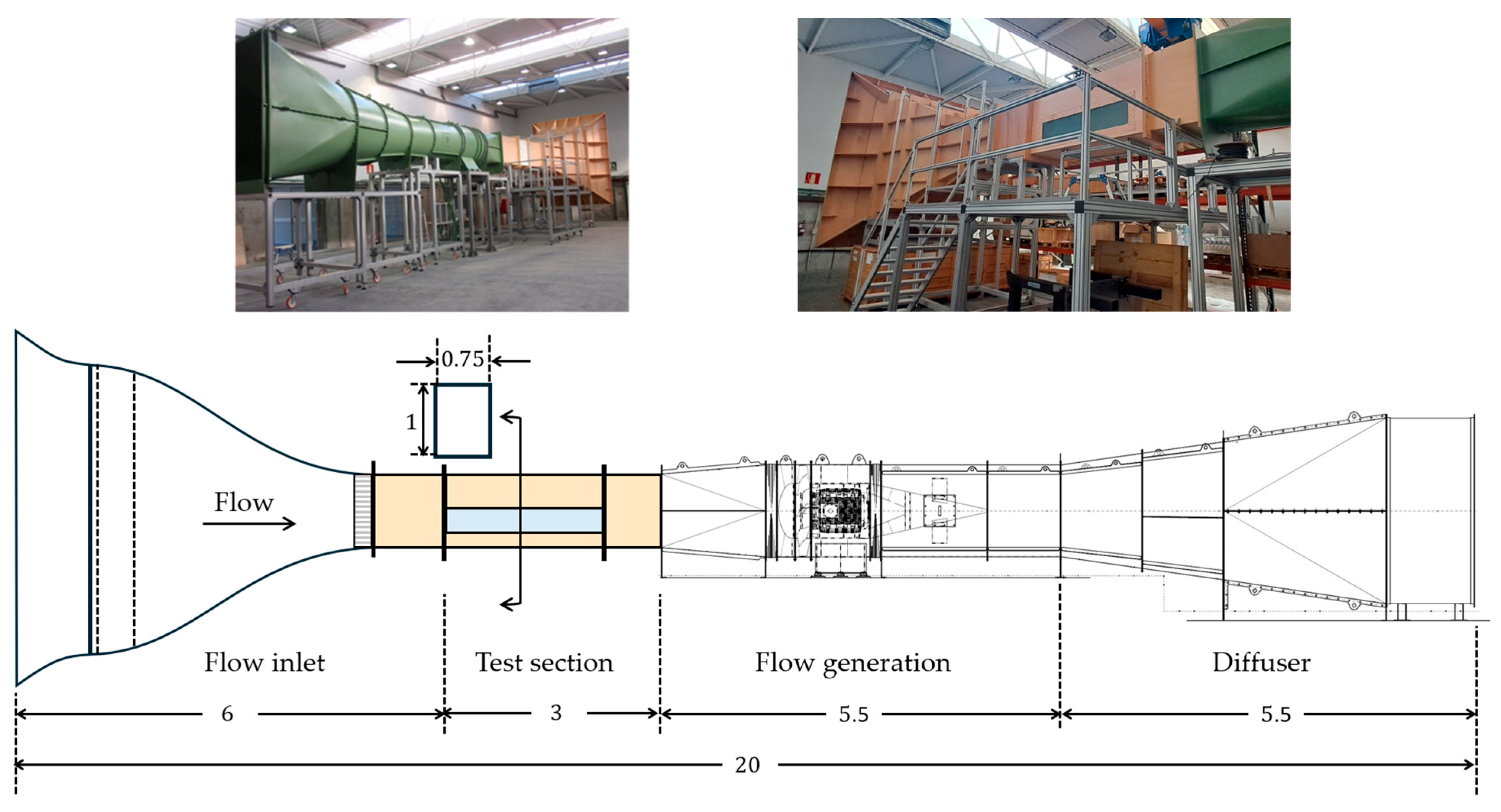
The facility to carry out the SHX scaled tests (Figure 6) is an open return, suction type wind tunnel operating at near-standard atmospheric conditions, with nominal free stream pressure, temperature and density respectively given by . The airflow is generated by an axial fan linked to a synchronous electric motor powered by a computer controlled, variable frequency drive. The test section, located downstream of a contraction, has a streamwise length with a rectangular cross section. At maximum drive, the free stream airflow velocity achieves a value close to , with a characteristic turbulent intensity . The integration of the SHX within the test section can be selected to best reproduce the key dimensionless parameters characterizing the nominal flight operation, in particular the turbulent boundary layer scales of the approaching flow defined at streamwise location . The SHX/airflow surface is to be placed horizontally across the span of the wind tunnel cross section and along its streamwise length, leading to a 1 m height between the SHX airflow exposed wall and the upper wind tunnel wall, which should establish a negligible streamwise pressure gradient due to boundary layer growth along the SHX extension.
Figure 6.
BV4 wind tunnel. Top: general view (left) and flow inlet and test section view (right). Bottom: longitudinal sketch with dimensions in .
As already mentioned, and according to the dimensional analysis presented in the previous section, physical similarity of the airflow established over the SHX between the flight operation and the wind tunnel scaled tests requires geometrical similarity of the SHX design and matching of the different key dimensionless parameters that appear in expression (18). These include the temperature ratio , and the Reynolds number . Denoting with subscripts respectively, the nominal flight and the wind tunnel operations, imposing the matching of these parameters implies:
Considering and the nominal flight operation values given in Table 1, fulfilling requirement (25a) leads to:
Assuming that the maximum free stream velocity is used in the wind tunnel tests and with , , requirement (25b) for Reynolds number matching establishes the length scale ratio between the two operating conditions:
The above expression indicates that the wind tunnel tests must be performed at a close to 2:1 length scale ratio relative to flight operation mode. Assuming that this scaling ratio is also applied to the sponson and to the SHX solid walls, and that a similar aluminum alloy is used for them in the flight and wind tunnel hardware, the ratio of the streamwise locations selected for the specification of the approaching flow conditions verifies:
Expression (28) indicates that the dimensionless position where the approaching flow boundary layer parameters should be matched is very similar in the wind tunnel and in the flight operation. Since the similarity in the boundary layer development establishes matching the values of the dimensionless streamwise coordinate, the dimensionless location to establish the approaching flow conditions for the wind tunnel tests will be approximated as:
For the wind tunnel tests, considering the above expression together with the values given in (24) and the 2:1 length scaling ratio found in (27) gives the following specification for the approaching turbulent boundary layer:
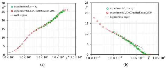
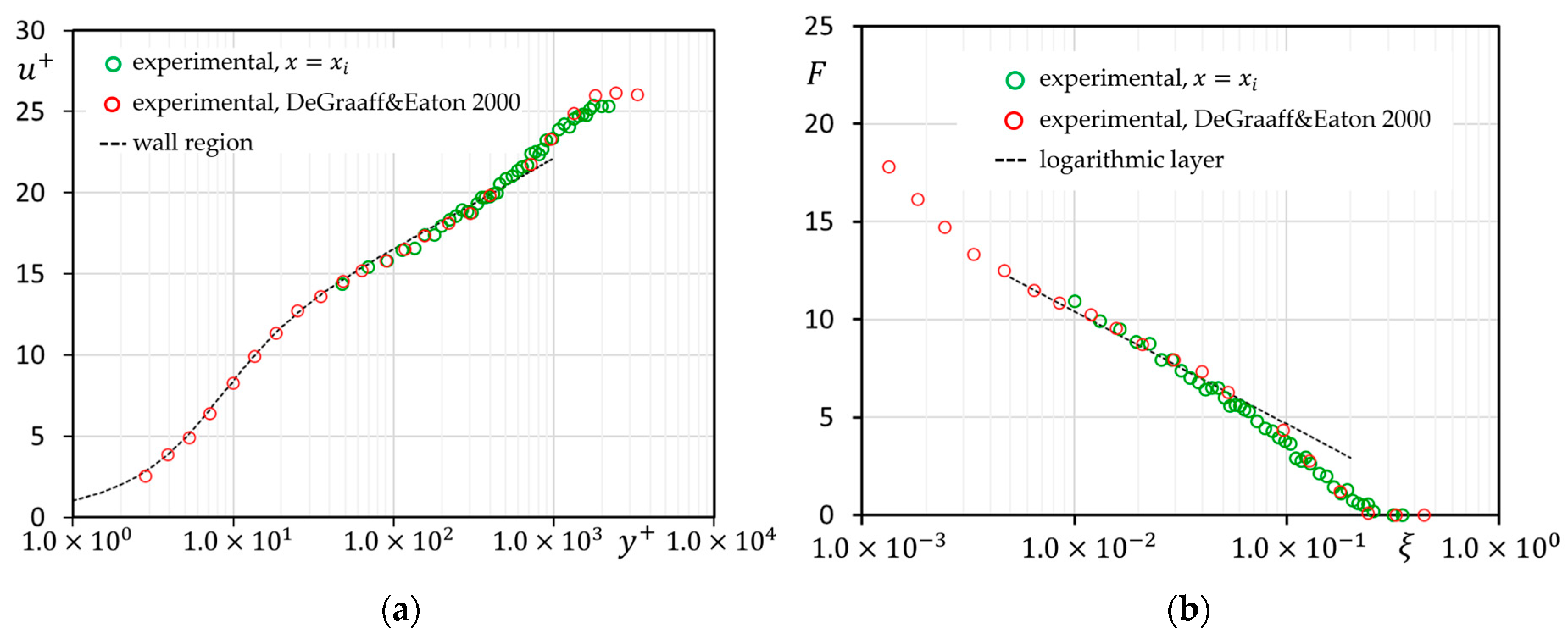
The location of streamwise station should be selected within the test section to give the boundary layer thickness and friction velocity established in expression (30) for the wind tunnel operating at the selected exterior velocity . Figure 7 shows hot-wire measurements conducted within the wind tunnel boundary layer, at the wind tunnel streamwise location selected to match the conditions given in (30).
Figure 7.
Approaching boundary layer velocity profiles for the wind tunnel tests, obtained at the streamwise location verifying (30). (a) Wall region scaling: DeGraaff & Eaton [34]; wall region [32]. (b) Velocity defect region scaling: Degraaff & Eaton [34]; logarithmic layer [35].
The wall region scaling gives the mean velocity and wall distance rendered dimensionless with wall magnitudes constructed from the exterior flow kinematic viscosity. For the velocity defect region, the scales are used to construct the dimensionless magnitudes:
Expression (30) provide for the wind tunnel data. The wind tunnel results are compared in Figure 7 to reference ZPG boundary layer experimental data obtained at [34], to the wall region description matching experimental data [32], and to the logarithmic layer scaling of the velocity defect layer [35]. The wind tunnel experimental data indicates that the approaching turbulent boundary layer compares well with the expected equilibrium profiles characterizing a ZPG turbulent boundary layer of similar development. Furthermore, the resulting turbulent scales obtained from this data provide an almost perfect match to the conditions given in (30). Specifically, the boundary layer scales obtained from the wind tunnel data shown in Figure 7 verify:
These results allow positioning the origin of the SHX in the wind tunnel tests that will be consistent with the expected turbulent properties of the airflow approaching the SHX in nominal flight operation.
Assuming that a similar aluminum alloy is used for the sponson and SHX solid walls in both wind tunnel tests and flight hardware, the following values of the dimensionless solid wall thermal conductivity are obtained:
The resulting values are close to each other and both . As already discussed, this should ensure a secondary effect of the specific value adopted by the solid wall dimensionless thermal conductivity on the airflow solution.
The imposed physical similarity between the nominal flight operation and the wind tunnel tests implies that similar results should be obtained for dimensionless parameters characterizing the airflow momentum and thermal boundary layers, and thus for the spanwise averaged friction coefficient , Stanton , and Nusselt numbers:
The magnitudes and that appear in the above definitions represent spanwise averaged values, since they are based in dimensionless airflow magnitudes that are also spanwise averaged. For the definition of the Stanton number, an effective exterior enthalpy is introduced, aimed at partially incorporating back the secondary role played by the exterior airflow Mach number:
For , the effective exterior enthalpy becomes the static exterior airflow enthalpy . This would be consistent with the approximate boundary layer Equation (5) that describes the limit . For , the effective exterior enthalpy becomes the stagnation enthalpy of the exterior airflow, which for a ZPG boundary layer would be the proper exterior reference enthalpy to define the Stanton number with non-negligible exterior Mach number effects. The value is then taken as a compromise to consider both limits. Finally, in the definition of the Nusselt number (34c), represents the streamwise coordinate of the virtual origin for the thermal boundary layer, defined as the streamwise station upstream of the SHX where the airflow surface heat flux drops to 1% of the peak value taking place at .
Table 2 summarizes the main parameters characterizing the airflow over the SHX for both the nominal flight operation and the wind tunnel scaled tests. The SHX length for the wind tunnels must be compatible with the test section space available in the BV4 wind tunnel, and is chosen as , equivalent to a SHX length for flight operation of
Table 2.
Main parameters characterizing the airflow over the SHX for the nominal flight operation and for the wind tunnel scaled tests.
4. CFD Validation of Wind Tunnel Test Scaling
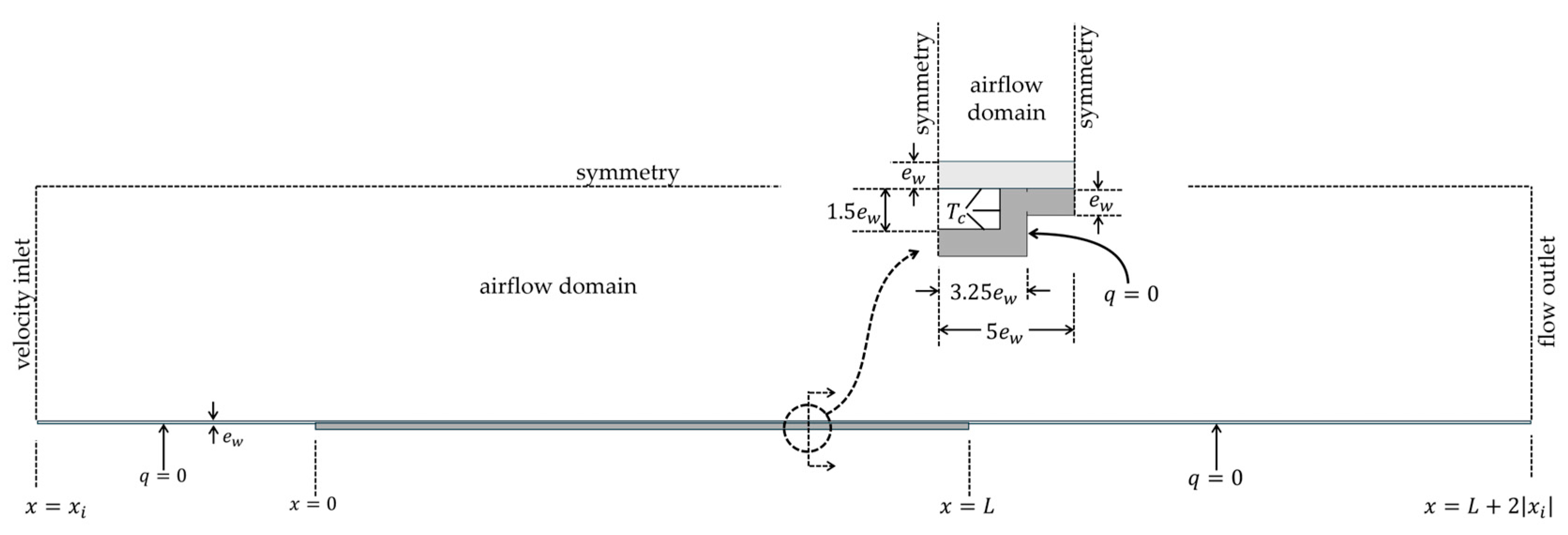
Numerical validation of the presented wind tunnel tests’ strategy can be carried out by CFD modeling of the airflow developing over a model of the SHX. A schematic view of the computational domain and boundary conditions used for these numerical studies is shown in Figure 8.
Figure 8.
CFD analysis of airflow development over SHX. Computational domain and boundary conditions for airflow and solid wall temperature development over SHX.
The computational domain includes thermal modeling of the sponson and SHX solid walls. Its inlet is located at the streamwise station where the approaching flow Reynolds number defined in (15a) matches both the flight operation and the wind tunnel tests. The temperature distribution in the solid walls is simultaneously solved by assuming an adiabatic boundary condition for the solid walls not exposed to airflow or to cooling fluid, and by setting a prescribed temperature at the cooling fluid channel.
Regarding the airflow, velocity inlet conditions including the inlet boundary layer with turbulent magnitudes are prescribed at . To properly model the inlet boundary layer, an independent numerical simulation is carried out on a ZPG boundary layer, and flow profiles obtained at the streamwise station of this simulation that match the inlet boundary layer thickness and friction velocity are taken as inlet boundary condition for the airflow. Symmetry conditions are applied at a cross-stream height , which matches the mid height of the wind tunnel cross section. Finally, a flow outlet boundary condition is prescribed at , which is considered sufficient to guarantee a negligible streamwise gradient of the flow, since according to expressions (9)–(11) a boundary layer developing under adiabatic wall should be established at distances of the order of downstream from the SHX trailing edge, and thus heat transfer effects should be significant only for streamwise stations verifying .
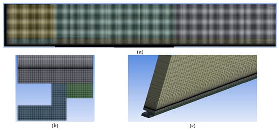
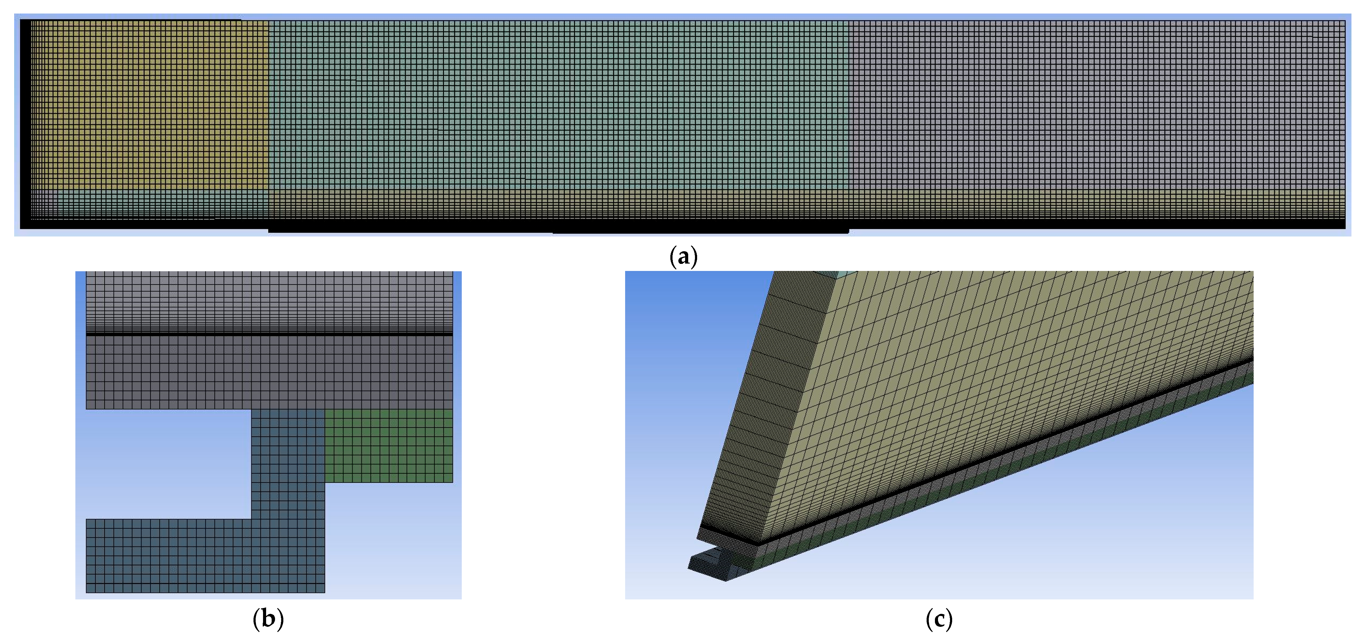
The numerical simulations were performed using the pressure-based solver of the CFD code Fluent from ANSYS version 2025R1, with second order discretization and coupled pressure–velocity treatment which allows the description of compressibility effects due to the airflow Mach number. The airflow was simulated with air taken as perfect gas. Two similar numerical grids were constructed to define the flight nominal and the wind tunnel test cases. Each numerical grid was developed around hexahedral cells and included clustering to properly resolve the boundary layer and possible streamwise gradients developing at the inlet region of the computational domain. Each resulting grid included a total of . The normal to wall size of the airflow cell in contact with the solid wall verifies , which allows resolving the viscous sublayer within the turbulent boundary layer.
Figure 9 shows some views of the numerical grid constructed for the airflow and for the sponson and SHX solid walls. Two-equation RANS models were selected to describe the turbulent flow development. Specifically, numerical simulations using both standard and SST models were performed to explore possible sensitivity of results obtained in the nominal flight and scaled test environments to the choice of the turbulent model. As the boundary layer develops under ZPG conditions, only local end thermal effects taking place at the leading and trailing edges of the SHX are expected to generate significant differences in the results of the numerical simulations using the two turbulence closures. Numerical simulations based on the model will be used to compare the airflow response in the nominal flight and scaled test environments. In addition, a comparison of wall friction and Stanton number given by the two different turbulence models will also be discussed.
Figure 9.
Details of the numerical grid used in the CFD validation studies. (a) Grid cut along the symmetry plane z = 0. (b) Cross-stream cut through the airflow wall region and SHX solid wall. (c) 3D view of the airflow near wall region and SHX solid wall.
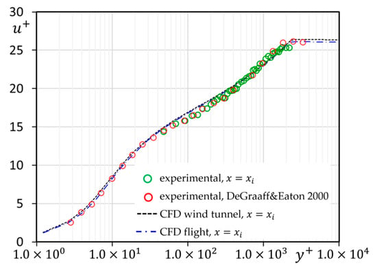
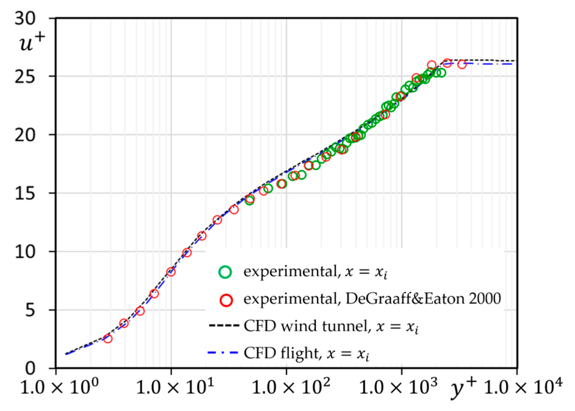
As already mentioned, for each turbulence model and operation environment, a precursor numerical simulation was performed over a ZPG boundary layer developing under adiabatic wall conditions, to obtain the flow profiles reproducing the boundary layer scales to be applied at the inlet of the computational domain shown in Figure 8. Figure 10 gives the mean velocity profiles resulting from the precursor simulation using the turbulence model, which reproduce the characteristics of a ZPG boundary layer and verify the turbulent scales set in Table 2 for the approaching boundary layer thickness and friction velocity. Almost identical profiles at the inlet are obtained when considering the SST turbulence closure. The results of the applied inlet velocity profiles for the CFD simulations of nominal flight and wind tunnel operation are very similar and practically coincide with the experimental data obtained in the assigned streamwise inlet coordinate for the experimental wind tunnel data.
Figure 10.
Mean velocity profile applied in the CFD numerical simulations at the inlet of the computational domain, . CFD inlet profiles given by the turbulence model for both nominal flight and wind tunnel scaled test environments, compared to wind tunnel experimental data obtained at the streamwise coordinate , and to reference experimental data for a ZPG adiabatic boundary layer of similar Reynolds number (DeGraaff & Eaton 2000, [34]).
A grid sensitivity analysis was performed to ensure grid independence in the CFD results. Starting with the reference grid described above, coarse and refined grids were constructed, characterized respectively by half and double spatial resolution in the three spatial coordinates.
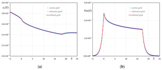
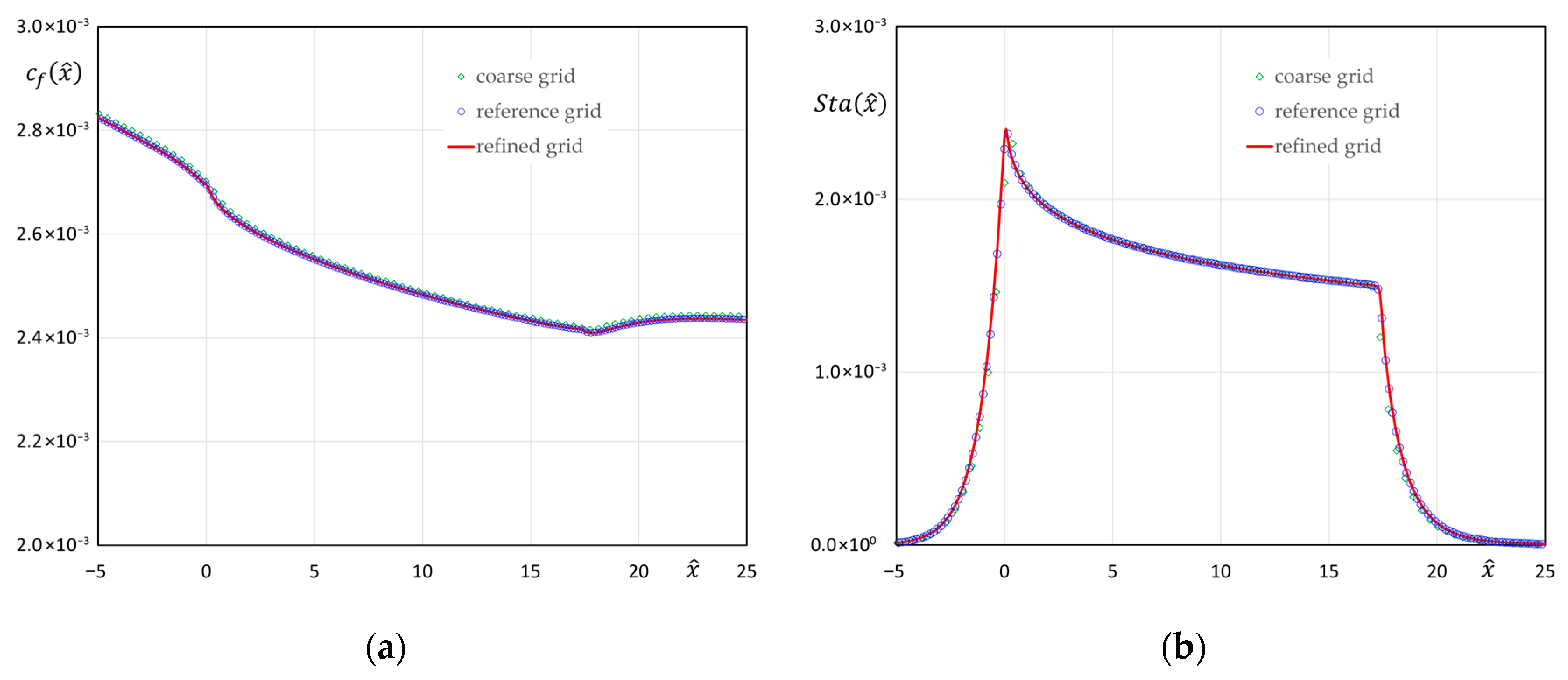
Figure 11 shows a comparison of the wall friction coefficient and Stanton numbers obtained using the turbulence model in the coarse, reference, and refined grids for the nominal flight operation environment. Whereas there is a slight difference between results given in the coarse and reference grids, the refined and reference grid results practically coincide, with similar trends also found using the SST turbulence model. Following these results, the reference grid will be used in the CFD analysis for the rest of the study.
Figure 11.
Grid sensitivity analysis performed for the turbulence model simulations. Dimensionless streamwise evolution of the wall friction coefficient and Stanton number for the nominal flight operation as given in the coarse, reference, and refined grids. (a) Wall friction coefficient. (b) Stanton number.
Table 3 summarizes the main characteristics of the boundary layer defined at the inlet dimensionless coordinate for both nominal flight and wind tunnel scaled test environments, confirming that the Reynolds number is closely matched between the different CFD simulations, and with the experimental wind tunnel data.
Table 3.
Main parameters defining the inlet boundary layer for the nominal flight and wind tunnel CFD simulations, and for the experimental wind tunnel conditions.
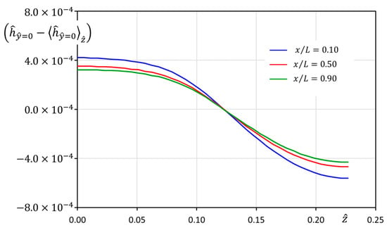
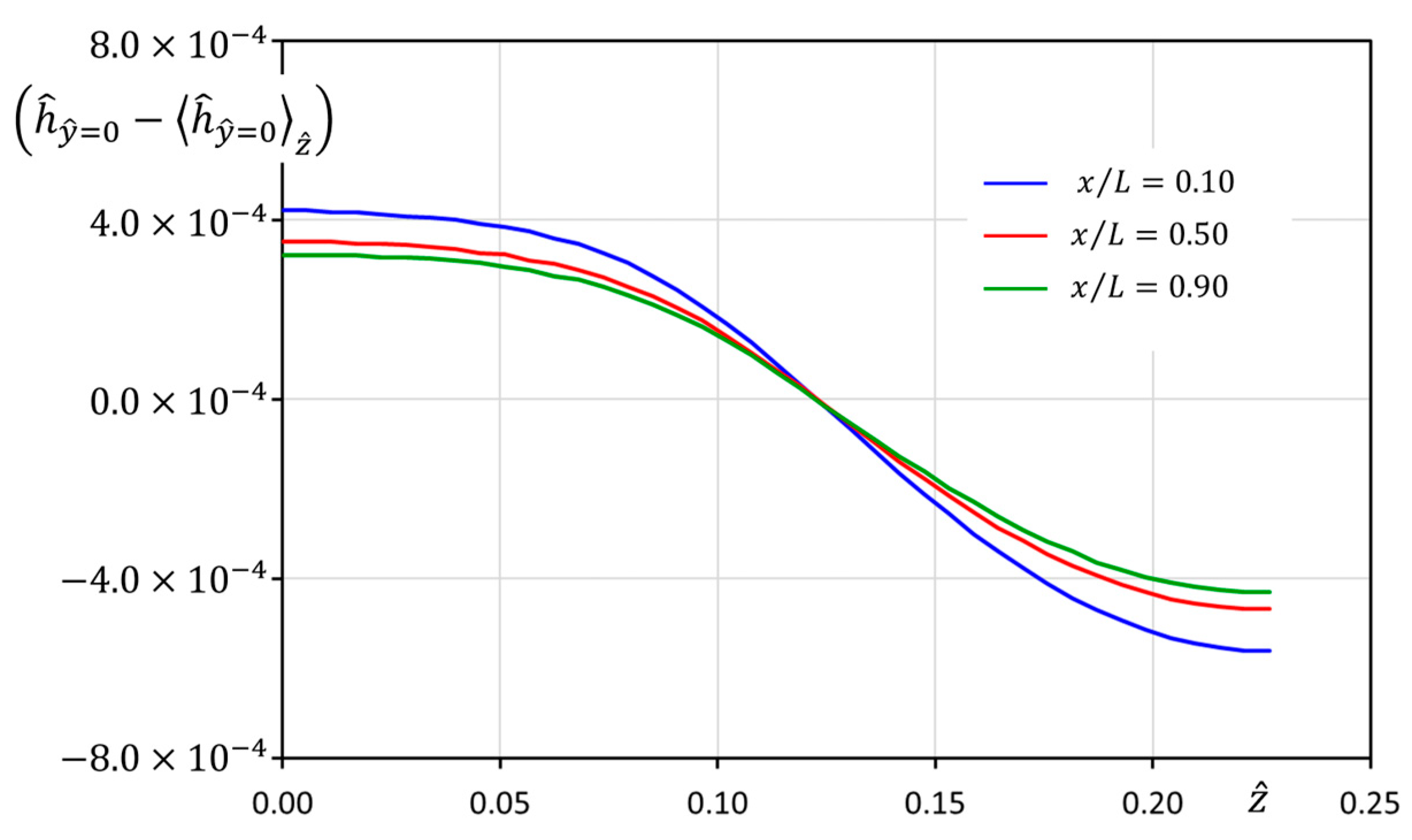
The assumption used in the study of the airflow having a weak spanwise dependence can be checked in Figure 12, showing the spanwise modulation of the dimensionless airflow enthalpy over the SHX solid wall at different streamwise locations. The results from the numerical simulations reveal that this modulation is , thus supporting the simplification introduced in the dimensional analysis presented above, based on averaging the mean airflow magnitudes along the spanwise coordinate.
Figure 12.
Spanwise modulation of the airflow wall enthalpy for nominal flight operation conditions at different streamwise locations.
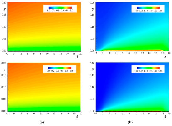
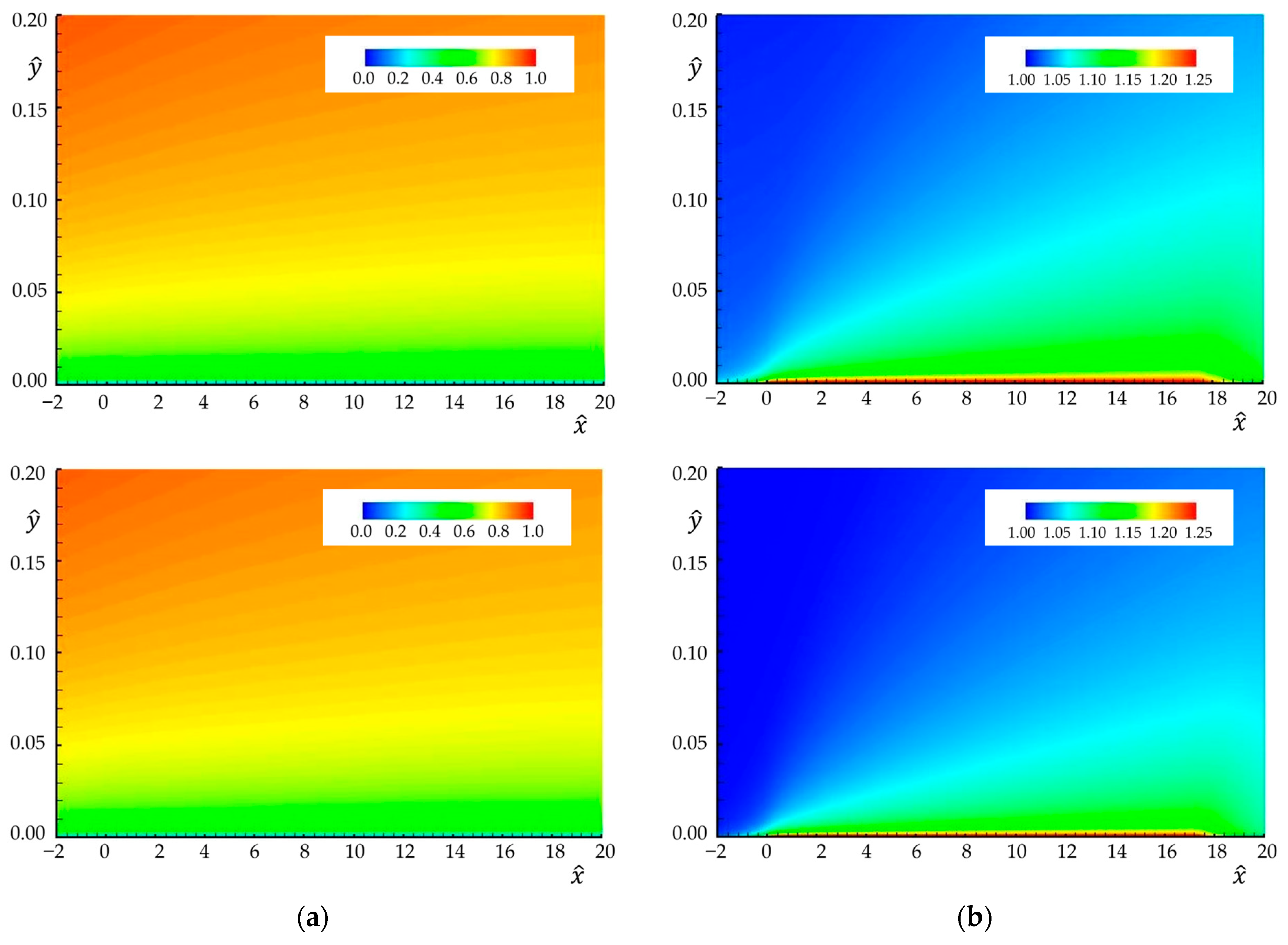
Dimensionless contour maps of the mean axial velocity and enthalpy developing over the SHX for both the nominal flight and scaled wind tunnel test environments are presented in Figure 13, where the dimensionless normal to wall distance has been greatly expanded to better show the boundary layer development.
Figure 13.
Contour maps of the CFD simulated boundary layer developing over the SHX. Results from turbulence model simulations. (a) Dimensionless mean axial velocity . (b) Dimensionless enthalpy . (Top): nominal flight environment. (Bottom): wind tunnel scaled test environment. SHX located in the segment .
The dimensionless mean velocity contour maps for the flight and wind tunnel scaled test environments exhibit a remarkable resemblance down to the wall layer, possibly indicating that the evolution of the friction coefficient should be very similar in both operating conditions. For the dimensionless enthalpy map, some differences are apparent in the external region of the thermal boundary layer, with somewhat higher levels at a given dimensionless wall distance characterizing the nominal flight results. This is to be expected as compressibility effects in the nominal flight simulation lead to residual temperature increases as the velocity is decreased in the external region of the boundary layer.
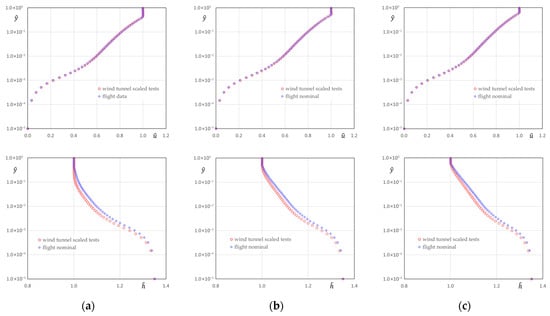
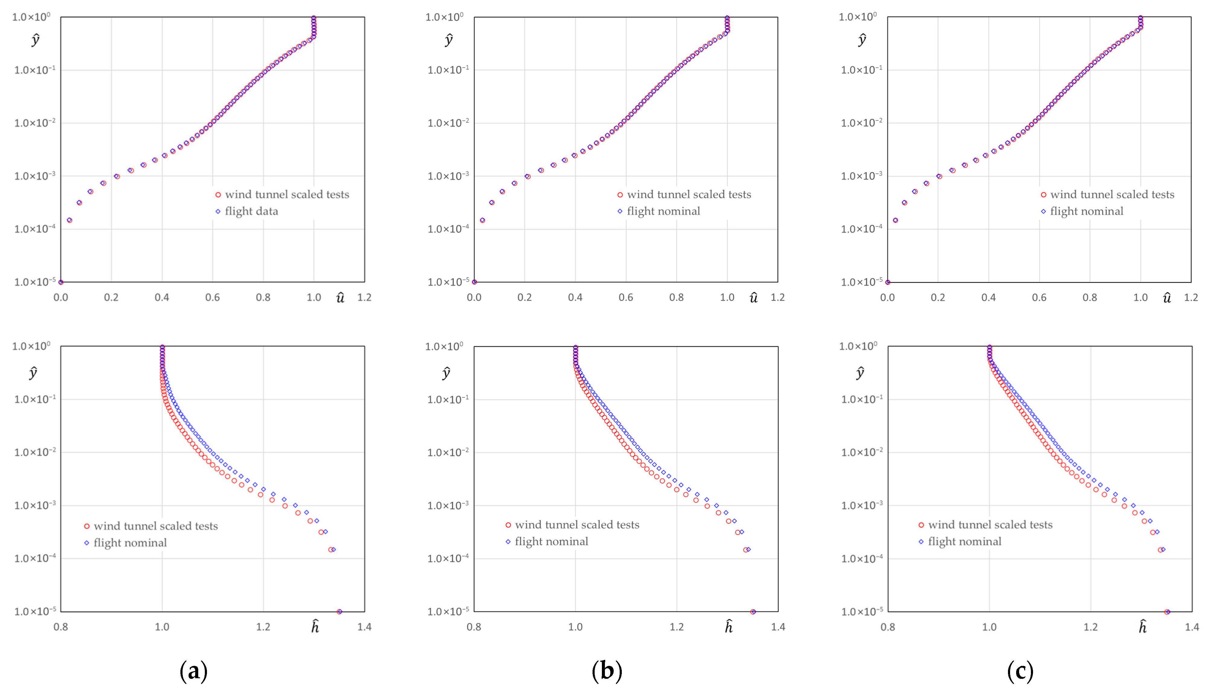
A more detailed analysis of these results can be derived by inspecting boundary layer profiles of the dimensionless mean velocity and enthalpy at specific locations over the SHX length. To this end, Figure 14 shows these profiles at coordinates or A logarithmic scale is used for the wall distance to highlight the wall layer, which defines the friction and heat transfer properties of the boundary layer. The mean velocity exhibits an almost perfect match for the two different environments in the different streamwise locations. Regarding the dimensionless enthalpy, the wall layer shows very similar, although some differences are revealed in the velocity defect region. As already mentioned, these differences are expected because of residual effects generated by the external Mach number in the nominal flight environment. Figure 14 also highlights the progressive streamwise evolution of the enthalpy profile in the velocity defect region, which tends to acquire a linear trend as it becomes progressively heated by the turbulent transport terms.
Figure 14.
Comparison of CFD results in the airflow boundary layer developing over the SHX for nominal flight and wind tunnel scaled test environments. (Upper row): dimensionless mean velocity profiles. (Lower row): dimensionless mean enthalpy profiles. (a) . (b) . (c) .
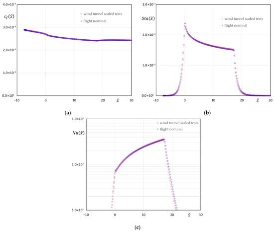
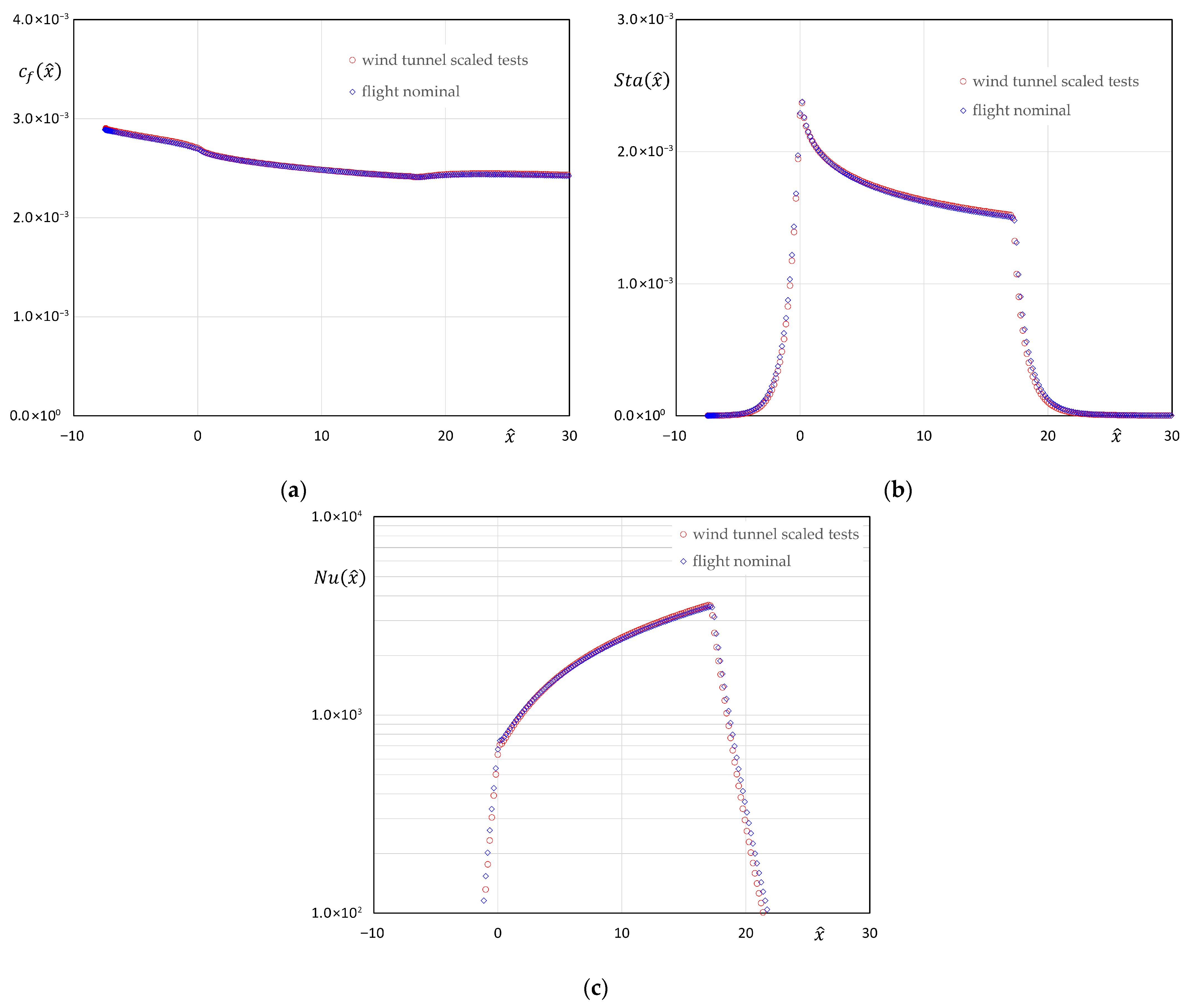
A confirmation of the global equivalence between the dimensionless airflow evolution for the nominal flight and wind tunnel scaled test environments is presented in Figure 15, showing the streamwise evolution of the wall friction coefficient and of the Stanton and Nusselt numbers defined in expression (34).
Figure 15.
Streamwise evolution of the spanwise averaged wall friction coefficient, Stanton, and Nusselt numbers in the SHX airflow boundary layer, showing CFD results from the flight nominal and wind tunnel test environment. (a) Wall friction coefficient. (b) Stanton number. (c) Nusselt number.
As expected from mean velocity results shown in Figure 14, the wall friction coefficient exhibits a remarkable equivalence in both environments. In addition, the definition of an effective exterior enthalpy given in (35) provides a way to compensate for the residual differences in the dimensionless enthalpy that appear in Figure 14. Figure 15 also gives information on the dimensionless relaxation distance that characterizes the heat transfer taking place upstream and downstream of the SHX, due to heating of the sponson wall. This value is compatible with the selected streamwise location defined in (24) to establish the approach flow conditions, which require negligible wall heat transfer effects. Integrating the data shown in Figure 15b and dividing it by the length of the SHX provides an average value of the Stanton number, which shows a difference between the nominal flight and the wind tunnel scaled tests. Finally, changing the value of the dimensionless solid wall thermal conductivity so that both environments share the value defined for the wind tunnel scaled tests leads to a negligible modification of the airflow magnitudes and thus of the SHX wall friction coefficient and of the Stanton and Nusselt numbers. This observation confirms the already suspected secondary role played by the parameter in the evolution of the airflow boundary layer developing over the SHX. All the above results seem to indicate the adequacy of the strategy proposed for the wind tunnel scale test program, aimed at providing a good assessment of the expected SHX thermal behavior in the nominal flight operation.
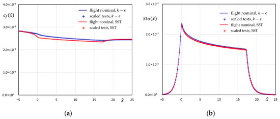
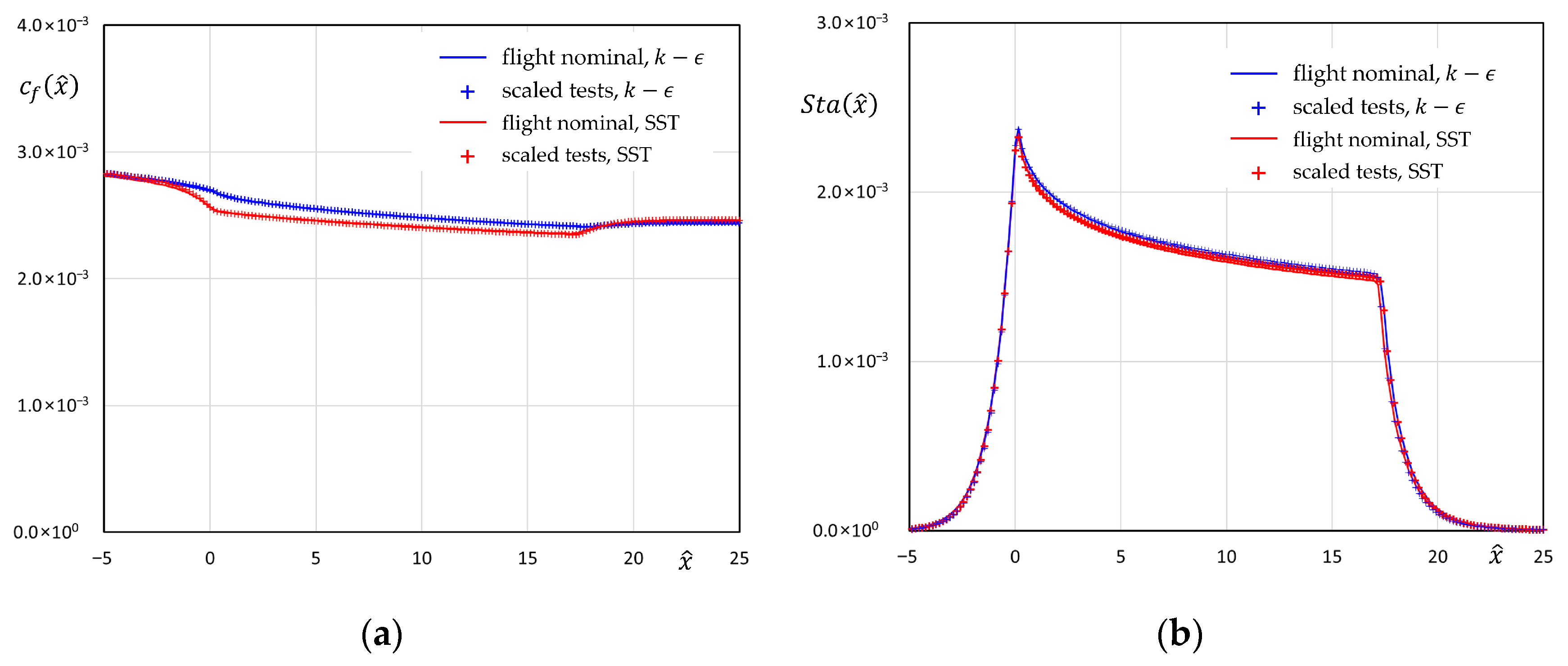
The impact of the turbulence model used in the numerical simulations is explored in Figure 16, where results for the friction coefficient and Stanton number given by the and SST models are shown for both the nominal flight and wind tunnel scaled test environments. Regarding the sensitivity of the CFD predictions to the turbulence closure, the streamwise evolution of the friction coefficient over the SHX shows a 5% decrease in the values given by the SST model with respect to the results produced by the turbulence model. The origin of these differences stems from the enhanced momentum boundary layer growth that the SST turbulent model gives at the leading edge of the SHX, where the boundary condition established over the cooling fluid channel leads to a sudden increase in the heat flux at the SHX wall in contact with the airflow. This localized heat flux peak generates a local growth in the momentum boundary layer and a corresponding decrease in the wall friction coefficient, with higher impact in the results given by the SST turbulence closure. The differences in the Stanton number given by the two turbulence closures are much smaller, with the SST turbulence model showing 1% decreases with respect to the closure in the region covered by the SHX surface.
Figure 16.
Streamwise evolution of wall friction coefficient and Stanton number given by and SST turbulence models in the flight nominal and wind tunnel scaled test environments. (a) Wall friction coefficient. (b) Stanton number.
Despite these differences, the friction coefficient and Stanton and Nusselt number given in the nominal flight and wind tunnel scaled test environments by the SST turbulence model show a similar trend to what was discussed for the numerical simulations, namely, a very close evolution of these parameters in the two different environments. Thus, the CFD validation of the wind tunnel test scaling procedure developed in the previous sections can be extended to results given by the SST turbulence closure.
5. Conclusions
Current conceptual studies performed for future HERA applications reveal a significant demand for thermal dissipation which should be ideally met while minimizing aerodynamic, weight, and energy penalties. In this context, SHXs that use the aircraft external airflow as a heat sink coupled to phase change cooling circuits provide an attractive means of partially meeting the challenges for heat dissipation. Presently, only conceptual studies have been developed to determine the potential of this technology. Increasing the present TRL beyond these studies requires undertaking an experimental test program in a relevant environment, that must strive to reproduce the operating conditions found in nominal flight operation. For SHX technology this implies reproducing the airflow velocity, pressure, temperature, and wall surface boundary layer development. Alternatively, the technology demonstration can be achieved using wind tunnel facilities operated at near-standard atmospheric conditions provided that physical similarity can be demonstrated between the two operation environments. In this context, the present study has established the following significant conclusions:
- The airflow Mach number plays a secondary role compared to the surface heating expected to take place over the SHX surface exposed to the airflow. This allows considering the use of low-speed wind tunnels to characterize the SHX thermal response.
- Except for local spanwise end effects, the SHX to airflow heat transfer is characterized by negligible spanwise modulation, leading to no significant three-dimensional boundary layer effects. This allows a two-dimensional analysis of the thermal and momentum boundary layers.
- The dimensional analysis of the airflow boundary layer leads to the identification of two critical dimensionless parameters controlling the SHX/Airflow heat transfer process, namely, the cooling flow to exterior airflow temperature ratio and the Reynolds number based on the external flow properties and the global turbulent boundary layer thickness of the flow approaching the SHX.
- Establishing the Reynolds number equivalence between nominal flight and wind tunnel test environments leads to fixing the geometrical scale between both operational conditions, defining the strategy to conduct scaled tests in a low-speed wind tunnel environment operated at near-standard atmospheric conditions.
- Using two-equation RANS turbulence closures, CFD numerical simulations validate the proposed scaled test strategy, leading to differences in the Stanton and Nusselt numbers between the wind tunnel tests and the nominal flight environments.
Author Contributions
Conceptualization, methodology, writing-original draft preparation, project administration, funding acquisition, B.J.L.; software, data curation, validation, E.G.-M. Writing-review and editing, investigation, resources, formal analysis, B.J.L. and E.G.-M. All authors have read and agreed to the published version of the manuscript.
Funding
This research was partially funded by Clean Aviation Joint Undertaking, grant agreement 101102008 Thermal Management for the Hybrid Electric Regional Aircraft (TheMa4HERA) under the Horizont Europe 2.5 Climate Energy and Mobility research program (https://cordis.europa.eu/project/id/101102008 accessed on 8 April 2026).
Data Availability Statement
Data are available on request from the authors.
Acknowledgments
The authors greatly acknowledge the support of the TheMa4HERA consortium partners for enabling the publication of this paper. Within this consortium, the authors are especially grateful to the interaction with the colleagues at Airbus Defence and Space-SA for providing the conceptual rendering of the SHX installation in HERA and preliminary data related to the SHX flight operation environment and geometry.
Conflicts of Interest
The authors declare no conflicts of interest.
Abbreviations
| CFD | Computational fluid dynamics |
| GHG | Green House Gas |
| HERA | Hybrid electric propulsion regional aircraft |
| HFO | Hydrofluoroolefin |
| ICAO | International Civil Aviation Organization |
| RANS | Reynolds averaged Navier–Stokes equations |
| SAF | Synthetic aviation fuel |
| SHX | Skin heat exchanger |
| SRIA | Strategic Research and Innovation Agenda |
| TPMS | Triply Periodic Minimal Surfaces |
| TRL | Technology Readiness Level |
| ZPG | Zero pressure gradient |
Nomenclature
| Mathematical accents | |
| Favre’s average | |
| Time average | |
| Dimensionless magnitude | |
| Subscripts | |
| e | Exterior airflow condition |
| ft | Nominal flight operation |
| i | Origin of the thermal boundary layer |
| wt | Nominal wind tunnel operation |
| Greek symbols | |
| ∆ | Global thickness of the turbulent boundary layer, [m] |
| Global thickness of the turbulent boundary layer at the origin of the thermal boundary layer, [m] | |
| SHX/airflow surface temperature deviation factor | |
| Heat capacity ratio | |
| Karman’s constant | |
| Molecular dynamic viscosity, | |
| Turbulent dynamic viscosity, | |
| Molecular kinematic viscosity, | |
| Molecular kinematic viscosity of the exterior airflow | |
| Surface of a boundary | |
| Surface of the solid wall–airflow boundary | |
| Surface of the solid wall–cooling channel boundary | |
| Surface of the solid wall not in contact with either the external airflow or the cooling fluid | |
| Dimensionless wall distance expressed in defect region scaling | |
| ) of SHX | |
| Regular nomenclature | |
| Effective exterior enthalpy factor | |
| Friction coefficient | |
| Dimensionless velocity defect expressed in defect region scaling | |
| Dimensionless velocity profile at the origin of the thermal boundary layer | |
| the surface of the solid wall–cooling channel boundary | |
| the surface of the solid wall not in contact with either the external airflow or the cooling fluid | |
| Mach number | |
| ] | |
| Exponent of the viscosity law as a function of the temperature | |
| Local value of the Nusselt number | |
| Prandtl number | |
| Turbulent Prandtl number | |
| Heat flux taking place at the SHX cooling channel wall, averaged over its cross-stream perimeter | |
| Local value of the Stanton number | |
| Characteristic value of the Stanton number SHX | |
| ] | |
| ] | |
| ] | |
| Cross-stream averaged sponson wall temperature, | |
| Turbulent intensity of the free stream | |
| Dimensionless flow velocity expressed in wall region scaling | |
| ] | |
| ] | |
| ] | |
| ] | |
| ] | |
| ] | |
| Dimensionless normal to wall distance expressed in wall region scaling | |
| Dimensionless normal to wall size of numerical grid cell expressed in wall region scaling |
References
- Kürten, B.; Cappelletto, M.; Zorgno, M.; Carpino, G.; Magnussøn, A.; Flæten, J.; Areng, M. Sustainable Blue Economy Partnership—Strategic Research and Innovation Agenda; Sustainable Blue Economy Partnership (SBEP): Brussels, Belgium, 2024. [Google Scholar] [CrossRef]
- Pettes-Duler, M.; Roboam, X.; Sareni, B. Integrated Optimal Design for Hybrid Electric Powertrain of Future Aircrafts. Energies 2022, 15, 6719. [Google Scholar] [CrossRef] [Scilit]
- Coutinho, M.; Afonso, F.; Souza, A.; Bento, D.; Gandolfi, R.; Barbosa, F.R.; Lau, F.; Suleman, A. A Study on Thermal Management Systems for Hybrid–Electric Aircraft. Aerospace 2023, 10, 745. [Google Scholar] [CrossRef] [Scilit]
- Coutinho, M.; Bento, D.; Souza, A.; Cruz, R.; Afonso, F.; Lau, F.; Suleman, A.; Barbosa, F.R.; Gandolfi, R.; Affonso, W.J.; et al. A review on the recent developments in thermal management systems for hybrid-electric aircraft. Appl. Therm. Eng. 2023, 227, 120427. [Google Scholar] [CrossRef] [Scilit]
- Broatch, A.; Olmeda, P.; García-Tíscar, J.; Felgueroso, A.; Chávez-Modena, M.; González, L.M.; Gelain, M.; Couilleaux, A. Experimental aerothermal characterization of surface air-cooled oil coolers for turbofan engines. Int. J. Heat Mass Transf. 2022, 190, 122775. [Google Scholar] [CrossRef] [Scilit]
- Broatcha, A.; García-Tíscar, J.; Felgueroso, A.; Chávez-Modena, M.; González, L.M.; Valero, E. Numerical and experimental analysis of rounded fins for high speed air-cooled heat exchangers. Int. J. Heat Mass Transf. 2023, 201, 123575. [Google Scholar] [CrossRef] [Scilit]
- Afonso, F.; Sohst, M.; Diogo, C.M.A.; Rodrigues, S.S.; Ferreira, A.; Ribeiro, I.; Marques, R.; Rego, F.F.C.; Sohouli, A.; Portugal-Pereira, J.; et al. Strategies towards a more sustainable aviation: A systematic review. Prog. Aerosp. Sci. 2023, 137, 100878. [Google Scholar] [CrossRef] [Scilit]
- Kellermann, H.; Habermann, A.L.; Hornung, M. Assessment of Aircraft Surface Heat Exchanger Potential. Aerospace 2020, 7, 1. [Google Scholar] [CrossRef] [Scilit]
- Haaland, S.E. Simple and Explicit Formulas for the Friction Factor in Turbulent Pipe Flow. J. Fluids Eng. 1983, 105, 89–90. [Google Scholar] [CrossRef] [Scilit]
- Incropera, F.P.; DeWitt, D.P.; Bergman, T.L.; Lavine, A.S. Principles of Heat and Mass Transfer, 7th ed.; International Student Version; Wiley: Singapore, 2013. [Google Scholar]
- Schultz-Grunow, F. New Frictional Resistance Law for Smooth Plates; Luftfahrtforschung: Bonn, Germany, 1940; Volume 17, pp. 239–246. Available online: https://digital.library.unt.edu/ark:/67531/metadc63129/m2/1/high_res_d/19930094430.pdf (accessed on 30 January 2026).
- Schlichting, H.; Gersten, K. Boundary-Layer Theory; Springer: Berlin/Heidelberg, Germany, 2017. [Google Scholar]
- Abreu, R.; Santos, P.; Afonso, F.; Suleman, A. A study on the potential of skin heat exchangers for hybrid-electric aircraft. Appl. Therm. Eng. 2025, 280, 128096. [Google Scholar] [CrossRef] [Scilit]
- Kallath, H.; Kholi, F.K.; Ha, M.Y.; Min, K.J.; Chetwynd-Chatwin, J. Computational Study on the Aerodynamics of a Surface-Heated Wing for Thermal Management. AIAA J. 2020, 58, 4339–4356. [Google Scholar] [CrossRef] [Scilit]
- Habermann, A.L.; Khot, A.; Lampl, D.E.; Perren, C. Aerodynamic Effects of a Wing Surface Heat Exchanger. Aerospace 2023, 10, 407. [Google Scholar] [CrossRef] [Scilit]
- Li, B.; Sun, Q.; Xiao, D.; Zhang, W. Numerical Investigation of the Aerofoil Aerodynamics with Surface Heating for Anti-Icing. Aerospace 2022, 9, 338. [Google Scholar] [CrossRef] [Scilit]
- Menter, F.R. Two-equation eddy-viscosity turbulence models for engineering applications. AIAA J. 1994, 32, 1598–1605. [Google Scholar] [CrossRef] [Scilit]
- Spalart, P.R.; Allmaras, S.R. A one-equation turbulence model for aerodynamic flows. In Proceedings of the 30th Aerospace Sciences Meeting and Exhibit, Reno, NV, USA, 6–9 January 1992. [Google Scholar] [CrossRef] [Scilit]
- Poinsatte, P.E. Heat Transfer Measurements from a NACA 0012 Airfoil in Flight and in the NASA Lewis Icing Research Tunnel; NASA Contractor Report 4278; NASA: Washington, DC, USA, 1990. Available online: https://ntrs.nasa.gov/citations/19900009887 (accessed on 28 January 2026).
- Felgueroso, A.; González-Nieves, I.; Díaz-Barja, M.; García-Rodríguez, J. Numerical modeling of a two-phase Skin Heat Exchanger for Hybrid-Electric Regional Aircraft. In Proceedings of the AIAA Aviation Forum and ASCEND, Las Vegas, NV, USA, 29 July–2 August 2024. [Google Scholar]
- Chaquet, J.M.; Torres, G. Efficient Phase-Change Fluid Model Applied to a Skin Heat Exchanger 3D Steady Thermal Simulation. In Proceedings of the TSAS2025: “Towards Sustainable Aviation” Summit, Toulouse, France, 28–30 January 2025. [Google Scholar]
- Shah, M.M. A General Correlation for Heat Transfer during Flow Condensation inside Pipes. Heat Mass Transf. 1979, 22, 547–556. [Google Scholar] [CrossRef] [Scilit]
- Torres, G.; Chaquet, J.M.; Jauntsarats, O.; Carrasco, D. Thermo-Mechanical Simulation of a Skin Heat Exchanger Considering Phase-Change Thermal Boundary Conditions. In Proceedings of the ASME Turbo Expo 2025, Turbomachinery Technical Conference and Exposition, Memphis, TN, USA, 16–20 June 2025; GT2025-151667; ASME: New York, NY, USA, 2025. [Google Scholar] [CrossRef] [Scilit]
- Oh, S.H.; Kim, J.E.; Jang, C.H.; Kim, J.; Park, C.Y.; Park, K. Multifunctional gradations of TPMS architected heat exchanger for enhancements in flow and heat exchange performances. Sci. Rep. 2025, 15, 19931. [Google Scholar] [CrossRef] [Scilit]
- Kaur, I.; Singh, P. State-of-the-art in heat exchanger additive manufacturing. Int. J. Heat Mass Transf. 2021, 178, 121600. [Google Scholar] [CrossRef] [Scilit]
- Favero, G.; Bonesso, M.; Rebesan, P.; Dima, R.; Pepato, A.; Mancin, S. Additive manufacturing for thermal management applications: From experimental results to numerical modeling. Int. J. Thermofluids 2021, 10, 100091. [Google Scholar] [CrossRef] [Scilit]
- Schaefer, S.; Quaium, F.; Muhsal, N.; Speerforck, A.; Thieleck, F.; Becker, C. Integration of a Cooling System Architecture with a Skin Heat Exchanger for High Thermal Loads in Fuel Cell Powered Aircraft. In Proceedings of the 19th International Refrigeration and Air Conditioning Conference, Purdue, IN, USA, 10–14 July 2022; Available online: https://docs.lib.purdue.edu/iracc/2347/ (accessed on 30 January 2026).
- Pang, L.P.; Dang, X.M.; Cheng, J. Study on Heat Transfer Performance of Skin Heat Exchanger. Exp. Heat Transf. 2015, 28, 317–327. [Google Scholar] [CrossRef] [Scilit]
- Larschow, M.T.; Thissen, S.; Gugliuzza, J.; Zistler, S.; Carosella, S.; Middendorf, P.; Poser, R. Concept of composite folded core skin heat exchanger with experimental investigation of surface temperatures using temperature-sensitive paints. Aerospace 2026, 13, 246. [Google Scholar] [CrossRef] [Scilit]
- Cebeci, T.; Bradshaw, P. Physical and Computational Aspects of Convective Heat Transfer; Springer: Berlin/Heidelberg, Germany, 1988. [Google Scholar] [CrossRef] [Scilit]
- Pirozzoli, S.; Smits, A.J. Outer-layer universality of the mean velocity profile in turbulent wall-bounded flows. Phys. Rev. Fluids 2023, 8, 064067. [Google Scholar] [CrossRef] [Scilit]
- Wilcox, D.C. Turbulence Modeling for CFD; DCW Industries: La Cañada, CA, USA, 2006; ISBN 978-1928729082. [Google Scholar]
- Tennekes, H.; Lumley, J.L. A First Course in Turbulence; MIT Press: Cambridge, MA, USA, 2018; ISBN 978-0262536301. [Google Scholar]
- DeGraaff, D.B.; Eaton, J.K. Reynolds-number scaling of the flat-plate turbulent boundary layer. J. Fluid Mech. 2000, 422, 319–346. [Google Scholar] [CrossRef] [Scilit]
- Pope, S.P. Turbulent Flows; Cambridge University Press: Cambridge, UK, 2000; ISBN 9780521598866. [Google Scholar]

Disclaimer/Publisher’s Note: The statements, opinions and data contained in all publications are solely those of the individual author(s) and contributor(s) and not of MDPI and/or the editor(s). MDPI and/or the editor(s) disclaim responsibility for any injury to people or property resulting from any ideas, methods, instructions or products referred to in the content. |
© 2026 by the authors. Licensee MDPI, Basel, Switzerland. This article is an open access article distributed under the terms and conditions of the Creative Commons Attribution (CC BY) license.