Shock-Aware Constrained Optimization of the RAE2822 Transonic Airfoil via a Two-Channel vSDF Surrogate with Closed-Loop CFD Verification

Abstract

Shock-aware aerodynamic shape optimization of transonic airfoils requires surrogate models that capture both integral aerodynamic trends and shock-relevant pressure distribution features. This study addresses drag-oriented optimization of the RAE2822 transonic airfoil under a lift-targeted condition with baseline relative thickness feasibility, rather than strict target pressure inverse design. Each airfoil is parameterized by a 16-dimensional CST vector and mapped to a two-channel vertical signed distance field representation of the upper- and lower-surface $C_p$ curves, from which shock descriptors, including the shock location indicator $x_s$ and the pressure jump magnitude $\Delta C_p$, are extracted in a deterministic, implementation-consistent manner. To quantify the reliability of surrogate-derived shock metrics, a held-out uncertainty analysis is performed on 500 samples. The surrogate achieves MAE/RMSE values of 0.00474/0.00602 for $C_L$ and $4.66\times {10}^{-4}/6.33\times {10}^{-4}$ for $C_D$, while the recovered shock-related quantities yield 0.00201/0.01598 for $x_s$ and 0.00200/0.00336 for $\Delta C_p$. Scatter plots and error histograms show tight one-to-one trends for most samples, with limited outliers mainly associated with locally ambiguous pressure gradient patterns. Overall, the surrogate is more reliable for capturing shock intensity trends than for prescribing an exact shock location; accordingly, $x_s$ is interpreted as a trend-level descriptor, whereas $\Delta C_p$ is treated as the more stable engineering indicator inside the optimization loop. The trained surrogate is embedded in a differential evolution optimizer with soft penalties on lift deviation and thickness feasibility violation, and selected designs are re-evaluated through closed-loop SU2 RANS simulations. CFD verification shows that the optimized design reduces drag from $C_D=0.01463$ to $C_D=0.01229$ (a 16.0% reduction) and reduces the shock jump from $\Delta C_p=0.239$ to $\Delta C_p=0.046$ (an 80.7% reduction). For the optimized design, the prediction-to-CFD differences are $\Delta C_L=+0.0042$ and $\Delta C_D=+0.00012$. These results support an engineering-oriented and auditable shock-aware closed-loop optimization workflow, with final design conclusions established by CFD verification rather than surrogate-predicted shock location alone.

1. Introduction

Transonic airfoil design remains a central problem in aerodynamic optimization because small geometric perturbations can alter shock location and shock strength, thereby changing wave drag levels and, in adverse cases, aggravating shock-induced boundary-layer interaction and loss of performance. Classical aerodynamic design theory established that gradient-based and control-theoretic frameworks can efficiently exploit high-dimensional design spaces, especially when coupled with adjoint information and high-fidelity flow solvers [1,2]. However, for practical transonic design, repeated viscous CFD evaluations are still computationally expensive, particularly when global exploration, multi-start search, trade-off analysis, or robustness-oriented studies are required. As a result, surrogate-based aerodynamic optimization has become an important route for reducing the number of expensive CFD calls while retaining acceptable physical fidelity for engineering decision-making [3,4,5,6,7].

At the methodology level, aerodynamic optimization performance depends not only on the optimizer itself but also on geometry parameterization, model fidelity management, and the treatment of design constraints. Parametric shape representations such as class-shape transformation (CST) provide compact and smooth descriptions of airfoil geometry and have become widely adopted in aerodynamic design [8,9]. On this basis, variable-fidelity and physics-informed surrogate strategies have been developed to accelerate shape optimization while preserving acceptable accuracy in the neighborhood of the design optimum [10,11,12,13,14,15,16]. In transonic applications, these considerations are especially important because feasibility requirements such as lift retention, thickness preservation, and low-speed or off-design constraints can strongly influence the practical relevance of a numerically optimized geometry [17,18].

With the rapid development of machine learning, data-driven aerodynamic analysis and optimization have advanced from conventional response-surface approximations to neural surrogates capable of predicting aerodynamic coefficients, surface pressure distributions, and even full flow fields. Early neural network studies demonstrated that data-driven models could support inverse design and rapid performance estimation for airfoils and wings [19]. Later work showed that machine learning could be integrated more directly into aerodynamic optimization pipelines through fast airfoil analysis, inverse design, gradient-enhanced neural surrogates, and data-efficient hybrid modeling strategies [7,20,21,22,23,24]. These developments substantially reduce marginal evaluation cost, but they also expose an important issue in transonic regimes: scalar-only prediction of $C_L$ or $C_D$ is often insufficient for trustworthy design guidance, because transonic performance is governed by localized pressure distribution features associated with shock formation, compression, and recovery.

Accordingly, recent studies have increasingly focused on predicting pressure distributions or flow fields rather than only integral coefficients. Deep-learning-based models have been used for rapid $C_p$ prediction on airfoils, supercritical-airfoil flow-field reconstruction, and transonic flow-field inference around airfoils [25,26,27,28]. More recent work has extended this direction to graph neural networks for surface pressure prediction on complex geometries, neural fields for aircraft aerodynamics, deep-learning frameworks for steady transonic flow-field prediction, probabilistic models emphasizing shock-wave regions, and predictive models specialized for transonic airfoil flow [29,30,31,32,33]. Operator-learning and physics-constrained latent models have also been introduced for supercritical-airfoil prediction tasks, further indicating that the field is moving from purely geometric regression toward physically structured flow representations [34]. Overall, the literature shows clear progress in fast aerodynamic inference, yet the requirements of engineering optimization remain stricter than those of standalone prediction: the surrogate must support reproducible feature extraction, stable optimization behavior, and credible closed-loop comparison against CFD.

In parallel, generative and inverse-design methods have opened another important branch of research. Conditional generative models, generative adversarial networks, and deep-learning-assisted global optimization have been used to synthesize airfoils or accelerate inverse design under prescribed performance tendencies [35,36,37,38,39]. These studies are highly relevant because they demonstrate how learned latent spaces can compress shape information, guide design search, and improve sampling efficiency. Nevertheless, many existing frameworks are oriented toward geometry generation, target matching, or direct field approximation, whereas practical transonic aerodynamic optimization often requires a more explicit linkage between predicted pressure distributions and shock-relevant engineering metrics. In other words, for drag-oriented transonic design, it is not enough to reconstruct a visually plausible pressure curve; the model must also support deterministic extraction of quantities that are physically meaningful for optimization, such as shock position indicators and shock-strength descriptors, while remaining auditable under closed-loop CFD verification.

These observations motivate the present study. Rather than treating transonic airfoil design as a strict target pressure inverse-design problem, this work addresses a drag-oriented aerodynamic shape optimization problem for the RAE2822 airfoil under a lift-targeted condition with baseline-relative thickness feasibility. The central idea is to use the pressure distribution as a physics-informative intermediate state, from which shock-related metrics can be extracted in a deterministic and code-consistent manner and then embedded into the optimization objective. It should be emphasized that, in the present dataset, sampled $C_p\left(x\right)$ values are indeed available directly from CFD post-processing. Therefore, the motivation for adopting an image-derived two-channel vSDF representation is not data accessibility per se, but the need for a regression target that is more suitable for shock-sensitive optimization. In transonic regimes, direct pointwise regression of $C_p\left(x\right)$ may be vulnerable to local oscillations or smeared discontinuity-like transitions near shocks, which can in turn reduce the robustness of downstream shock metric extraction. By contrast, the proposed vSDF representation converts the pressure curves into a smoother field while preserving their geometric structure through the zero-level sets of the upper and lower channels. This makes the representation particularly convenient for deterministic curve recovery and reproducible computation of shock-related descriptors within the optimization loop. The present work therefore adopts the vSDF formulation as an engineering-oriented representation choice for robust feature recovery, rather than claiming that it is universally superior to all direct $C_p\left(x\right)$ regression strategies. To this end, each airfoil is parameterized by a 16-dimensional CST vector, and a multi-task surrogate is trained to predict both aerodynamic coefficients and a two-channel vertical signed distance field (vSDF) representation of the upper- and lower-surface $C_p$ curves. This representation is designed to stabilize the learning and recovery of pressure distribution features with sharp local gradients, which is essential in transonic flows where shock signatures dominate the drag trend. The surrogate is then embedded into a differential evolution optimizer with soft penalties on lift deviation and thickness feasibility violation, and the resulting candidate designs are re-evaluated by SU2 RANS in a closed loop.

The main contributions of this work are as follows. First, a two-channel vSDF representation of upper- and lower-surface $C_p$ curves is introduced for transonic airfoil surrogate modeling, enabling stable curve recovery and reducing sensitivity to rendering-style variations. Second, a deterministic and implementation-consistent procedure is established to extract shock-related descriptors from the recovered pressure distribution, allowing the optimization to penalize shock intensity in a reproducible manner. Third, an engineering-oriented closed-loop CFD verification workflow is constructed so that surrogate-guided improvements can be assessed against high-fidelity RANS results rather than remaining at the surrogate-only level. Under this formulation, the present work emphasizes auditable drag reduction with shock mitigation and feasibility preservation, instead of claiming exact prescription of an absolute shock location.

The remainder of this paper is organized as follows. Section 2 presents the dataset construction, geometry parameterization, surrogate architecture, shock metric extraction procedure, optimization formulation, and CFD verification strategy. Section 3 reports surrogate accuracy, optimization results, trade-off behavior, and closed-loop CFD validation. Section 4 discusses the engineering implications and limitations of the proposed workflow, and Section 5 summarizes the main conclusions.

2. Methodology

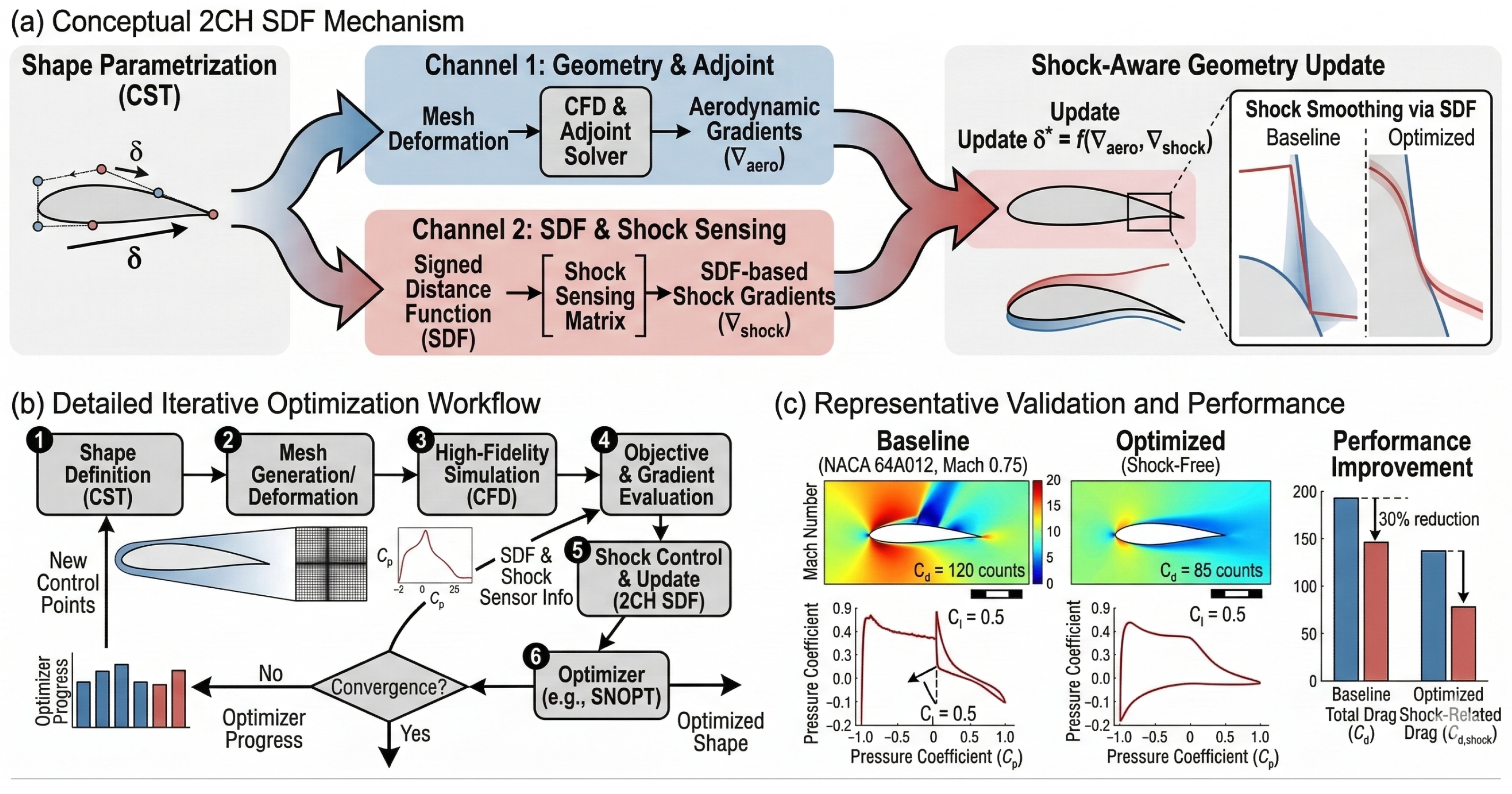
Section 2 describes the end-to-end workflow summarized in Figure 1. Starting from SU2 RANS simulations, we build a cached dataset containing CST parameters, aerodynamic coefficients, and consistent $C_p$-plot images. A multi-task surrogate is trained to map CST inputs to a two-channel vSDF pressure representation and to $(C_L,C_D)$. The surrogate is then embedded into a differential evolution optimizer under a lift-targeted, soft-penalty feasibility formulation. Finally, selected optimized designs are re-meshed and re-evaluated using SU2 RANS in a closed loop, and post-processing scripts generate publication-ready comparisons between surrogate predictions and CFD results.

The canonical notation used throughout the paper is summarized in

Table 1. Canonical notation used throughout the paper.

Symbol/Label	Meaning
$\mathrm{Pred}$/$\mathrm{CFD}$/$\mathrm{GT}$	surrogate prediction/CFD verification/ground truth (dataset)
$C_L,C_D$	lift and drag coefficients
$x_s$	shock location extracted from recovered upper-surface $C_p\left(x\right)$
$\Delta C_p$	shock-jump magnitude (code-consistent neighborhood average)
S	shock score (top-fraction mean of $|d{C}_p/dx|$ in window)
$J\left(a\right)$	scalarized objective with soft penalties (lift targeting + thickness feasibility)

.

2.1. Problem Setup and Data

This work targets shock-aware scalarized optimization with soft-penalty feasibility for the RAE2822 transonic airfoil under a fixed operating condition consistent with the SU2 RANS setup used to generate the dataset (

Table 2. Dataset summary and CFD operating condition used in this work. Grid statistics (cell/node counts and representative wall-resolution indicators) are reported for reproducibility.

Category	Item	Value/Source
Dataset	Number of samples N	5000
Dataset	CST dimension	16 (8 upper + 8 lower)
Dataset	$C_p$ plot resolution	$512\times 512$
CFD condition	Solver/turbulence model	RANS/SST
CFD condition	Mach number	0.729
CFD condition	Reynolds number	$6.5\times {10}^6$
CFD condition	Angle of attack (deg)	2.31
CFD condition	Free-stream temperature (K)	288.15
CFD condition	Grid size	$N_{\mathrm{cells}}=17,839$, $N_{\mathrm{nodes}}=12,778$
CFD condition	$Y^{+}$	1.341

). Airfoil geometry is parameterized by a 16-dimensional CST vector $\mathbf{a}\in {\mathbb{R}}^{16}$ (8 coefficients for the upper surface and 8 for the lower surface). For each sampled geometry, SU2 provides supervision signals including (i) aerodynamic coefficients $(C_L,C_D)$ and (ii) a rendered $C_p$ plot image. The dataset contains $N=5000$ CST-perturbed airfoils around the RAE2822 baseline, generated with controlled, bounded coefficient perturbations and basic geometric sanity checks (e.g., non-negative thickness and smooth trailing-edge behavior). For reproducibility, the CST perturbation bounds and rejection criteria are recorded together with the cache metadata. Specifically, each coefficient is sampled within prescribed bounds $a_i\in [a_i^{min},a_i^{max}]$ (exported in cst_bounds.json), and a candidate geometry is rejected if it violates any of the following deterministic checks on a fixed chordwise grid: (i) non-negative thickness $t\left(x\right)\ge 0$ for all sampled x; (ii) no near-singular thickness segments (to prevent mesh collapse); and (iii) smooth trailing-edge behavior under the adopted CST/TE parameterization. These rules prevent non-physical shapes and reduce solver failure bias in the supervised dataset while keeping the sampling neighborhood engineering-relevant. The dataset is split into training/validation/test subsets with ratios $0.8/0.1/0.1$ using a fixed random seed for reproducibility.

The adoption of an image-based $C_p$ extraction pipeline—while seemingly indirect when raw CFD data are available—is deliberately engineered to ensure broader forward compatibility. This pipeline enables ingestion and vectorization of legacy aerodynamic data from historical literature, where only graphical plots are accessible, thereby expanding the surrogate’s applicability in practical engineering scenarios.

2.2. Grid Independence Study

Prior to executing the closed-loop optimization, a grid independence study was conducted on the baseline RAE2822 airfoil. Three grids (coarse/medium/fine) with $N_{\mathrm{cells}}=7500/18,000/30,000$ were evaluated. The medium grid was selected because the medium-to-fine relative differences were below $0.2\%$ for both $C_L$ and $C_D$, while providing a practical turnaround time for the closed-loop verification.

2.3. From $C_p$ Image to Two Curves and Two-Channel Vertical SDF (vSDF)

To enable stable learning of sharp transonic features (e.g., shocks), the $C_p$ plot image is converted into two 1D curves and then into a compact field representation. It is noted that direct numerical regression of sampled $C_p\left(x\right)$ is also feasible in principle, since the CFD data provide the pressure distribution explicitly. However, for the present shock-aware optimization task, the representation is required not only to reconstruct the pressure curve itself, but also to support robust downstream extraction of local shock-related descriptors. In transonic conditions, pointwise regression of $C_p\left(x\right)$ may be sensitive to steep local gradients and can produce locally oscillatory or overly smoothed predictions near shock regions, which are unfavorable for stable estimation of quantities such as shock position indicators and pressure jump magnitude. The proposed two-channel vSDF representation instead maps the upper and lower pressure curves into bounded signed-distance-like fields whose zero-level sets retain the target curve geometry, while the field itself remains smoother and more regression-friendly. We therefore adopt this representation as an optimization-oriented compromise between geometric fidelity, numerical stability, and deterministic post-processing consistency.

2.3.1. Extract Upper/Lower $C_p$ Curves from the $C_p$ Image

From a cropped $C_p$ curve panel with a uniform background, curve pixels are detected by simple intensity thresholding and color filtering. For each chordwise image column, the topmost detected curve pixel defines the upper-surface trace $y_u\left(x\right)$, and the bottommost pixel defines the lower-surface trace $y_l\left(x\right)$. Columns with missing detections are filled by linear interpolation in x, and the resulting discrete traces are smoothed with a short moving-average filter to suppress isolated pixel noise while preserving the shock-induced jump structure.

2.3.2. Build a Vertical Signed Distance Field (vSDF) for Each Curve

For each curve trace $y_{\mathrm{curve}}\left(x\right)$ defined on the image grid (with $y=0$ at the top row), a vertical signed distance field $\mathrm{vSDF}(y,x)$ is constructed as

$$\mathrm{vSDF}(y,x)=\mathrm{clip}\left({\displaystyle \frac{y-y_{\mathrm{curve}}\left(x\right)}{\beta }}, -1, 1\right),$$

(1)

where $\beta$ (set to $\beta =12$ pixels in this work) scales the signed vertical distance to a normalized range, and $\mathrm{clip}(·)$ bounds the target field to $[-1,1]$ for numerically stable learning. Stacking the upper and lower channels yields the two-channel target field

$${\mathrm{SDF}}_2(y,x)=\left[{\mathrm{vSDF}}_{\mathrm{upper}}(y,x),{\mathrm{vSDF}}_{\mathrm{lower}}(y,x)\right].$$

(2)

This representation preserves curve geometry while providing a smooth, regression-friendly field whose zero level set corresponds to the target curve.

The corresponding vSDF conversion and curve-recovery pipeline is illustrated in Figure 2.

2.4. Multi-Task Surrogate: CST(16) $\to \{2\mathrm{ch}\mathrm{vSDF},C_L,C_D\}$

A single neural surrogate is trained to predict both the pressure distribution representation and the aerodynamic coefficients:

• Input: CST vector $\mathbf{a}\in {\mathbb{R}}^{16}$ (normalized to zero mean and unit variance using training-set statistics).
• Outputs: predicted two-channel vSDF field ${\widehat{\mathrm{SDF}}}_2$ and scalar coefficients $({\widehat{C}}_L,{\widehat{C}}_D)$.

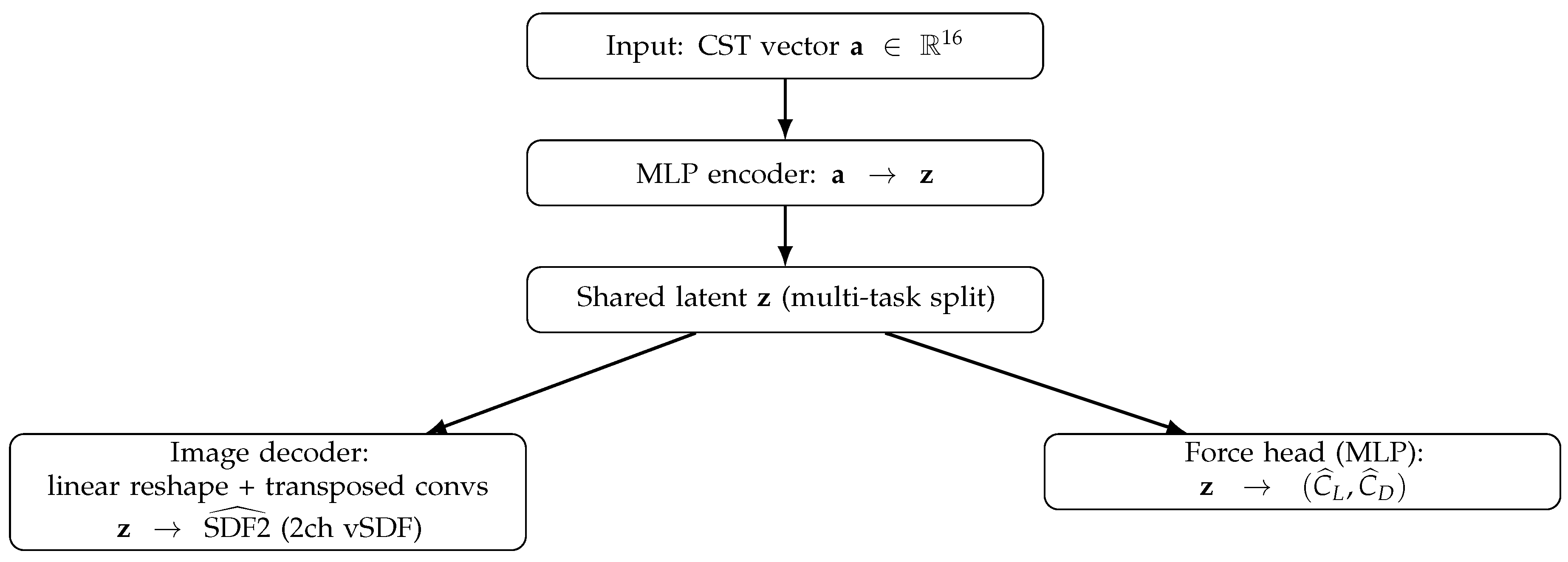
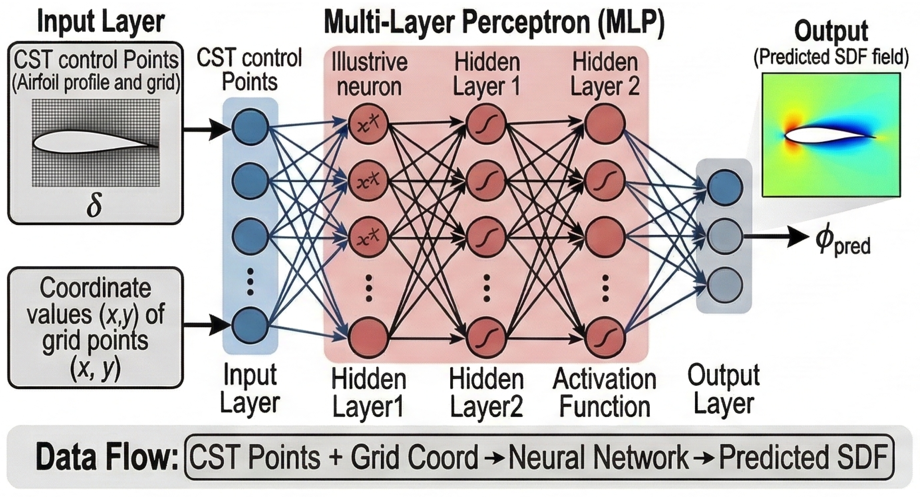
As illustrated in Figure 3, the network uses a shared latent representation produced by an MLP encoder, which is decoded by an image-field decoder into ${\widehat{\mathrm{SDF}}}_2$ while a lightweight regression head predicts $({\widehat{C}}_L,{\widehat{C}}_D)$. The vSDF output is bounded by a $tanh(·)$ activation to match the target range $[-1,1]$.

Implementation summary. (i) An MLP maps $\mathbf{a}$ to a latent vector $\mathbf{z}$. (ii) A linear projection reshapes $\mathbf{z}$ into a small spatial feature map of size $(C\times G\times G)$ with $G=8$ by default. (iii) A sequence of transposed convolutions upsamples features to the target resolution (e.g., $512\times 512$), using GroupNorm and SiLU activations with lightweight residual blocks. (iv) A final 2-channel convolution produces ${\widehat{\mathrm{SDF}}}_2$. (v) A separate MLP head regresses $({\widehat{C}}_L,{\widehat{C}}_D)$ from $\mathbf{z}$.

A simplified task-flow view of the same surrogate is shown in Figure 4.

2.5. Training Loss Functions

The training objective combines image-field fidelity and force regression to ensure that the surrogate is accurate both in integral coefficients and in shock-relevant pressure features. The overall loss is defined as

$$\mathcal{L}=w_{\mathrm{sdf}}{\mathcal{L}}_{\mathrm{sdf}}+w_{\mathrm{grad}}{\mathcal{L}}_{\mathrm{grad}}+w_{\mathrm{sign}}{\mathcal{L}}_{\mathrm{sign}}+w_{\mathrm{force}}{\mathcal{L}}_{\mathrm{force}},$$

(3)

where $(w_{\mathrm{sdf}},w_{\mathrm{grad}},w_{\mathrm{sign}},w_{\mathrm{force}})$ are fixed scalar weights, and all loss weights and scaling constants (including $w_{\mathrm{lower}}$ and ${\lambda }_{cd}$) are listed explicitly in

Table 3. Reproducibility table of surrogate loss weights and scaling constants (implementation-consistent).

Symbol/Name	Meaning	Value in This Work
$w_{\mathrm{sdf}}$	vSDF regression weight in Equation (3)	1.0
$w_{\mathrm{grad}}$	Gradient consistency weight in Equation (3)	0.10
$w_{\mathrm{sign}}$	Sign consistency weight in Equation (3)	0.15
$w_{\mathrm{force}}$	Force regression weight in Equation (3)	0.20
$\alpha$	Near-curve focusing in Equations (4) and (5)	10
k	Sign margin sharpness in Equation (7)	10
${\lambda }_{cd}$	Drag scaling in Equation (8)	100
$w_{\mathrm{lower}}$	Extra weight on lower-channel image losses	0.5
Huber $\beta$	Huber transition parameter in Equation (8)	0.5

for reproducibility.

2.5.1. vSDF Regression Loss (Weighted SmoothL1)

To emphasize accuracy near the curve (i.e., near the zero level set where $\mathrm{SDF}\approx 0$), a distance-based weight is applied so that errors close to the curve are penalized more heavily:

$$w(y,x)=exp\left(-\alpha \left|{\mathrm{SDF}}_{\mathrm{GT}}(y,x)\right|\right),$$

(4)

$${\mathcal{L}}_{\mathrm{sdf}}=\mathbb{E}\left[w·\mathrm{SmoothL1}\left({\mathrm{SDF}}_{\mathrm{Pred}},{\mathrm{SDF}}_{\mathrm{GT}}\right)\right],$$

(5)

where $\alpha$ is a focusing coefficient (set to $\alpha =10$ in this work) that balances near-curve fidelity and numerical stability.

2.5.2. Gradient Consistency Loss

To improve local geometric consistency of the predicted fields, we additionally match finite-difference gradients in both x and y directions:

$$L_{\mathrm{grad}}=\mathrm{SmoothL1}\left({\nabla }_x{\mathrm{SDF}}^{\mathrm{Pred}}-{\nabla }_x{\mathrm{SDF}}^{\mathrm{GT}}\right)+\mathrm{SmoothL1}\left({\nabla }_y{\mathrm{SDF}}^{\mathrm{Pred}}-{\nabla }_y{\mathrm{SDF}}^{\mathrm{GT}}\right).$$

(6)

2.5.3. Sign Consistency via BCE on SDF Sign

Because the vSDF sign indicates whether a pixel lies above or below the curve, a sign consistency term is included to discourage sign flips that can corrupt curve recovery. We use a logistic classification loss on the sign:

$${\mathcal{L}}_{\mathrm{sign}}=\mathbb{E}\left[w·\mathrm{BCEWithLogits}\left(-k{\mathrm{SDF}}_{\mathrm{Pred}},\mathbb{I}({\mathrm{SDF}}_{\mathrm{GT}}\le 0)\right)\right],$$

(7)

where k controls the margin sharpness (set to $k=10$ in our implementation) and $\mathbb{I}(·)$ denotes the indicator function.

2.5.4. Force Regression Loss

The force regression loss incorporates both lift and drag. Since $C_D$ is typically two orders of magnitude smaller than $C_L$, a scaling factor ${\lambda }_{cd}$ is applied to prevent the drag term from being under-emphasized:

$${\mathcal{L}}_{\mathrm{force}}=\mathrm{Huber}\left({\widehat{C}}_L-C_L\right)+\mathrm{Huber}\left({\lambda }_{cd}\left({\widehat{C}}_D-C_D\right)\right),$$

(8)

with ${\lambda }_{cd}=100$ in this work.

Quantitative prediction diagnostics for shock-related quantities are reported in the Section 3.

2.6. Shock Metric Extraction and Engineering Alignment

A key requirement for shock-aware optimization is an automatic and reproducible shock indicator derived from the predicted pressure distribution. In this work, the shock metrics are extracted from the recovered upper-surface $C_p\left(x\right)$ curve using a fixed procedure consistent with the implementation, thereby enabling both surrogate-driven optimization and consistent comparison with CFD post-processing.

2.6.1. Recover $C_p$ Curve from vSDF (Soft-Argmin)

For each chordwise location x, the curve pixel coordinate $y\left(x\right)$ is recovered by a soft-argmin over $\left|\mathrm{SDF}\right(y,x\left)\right|$, which provides a smooth and robust alternative to a hard $argmin$:

$$w\left(y\right)=exp\left(-\kappa \left|\mathrm{SDF}\right(y,x\left)\right|\right),y\left(x\right)={\displaystyle \frac{{\sum }_{y}w\left(y\right)y}{{\sum }_{y}w\left(y\right)}},$$

(9)

where $\kappa$ controls the sharpness of the recovery (set to $\kappa =25$ in this work).

2.6.2. Map Pixel y to $C_p$ and Smooth

After recovering the curve pixel coordinate $y\left(x\right)$ on an image of height H, we map it to $C_p\left(x\right)$ using the same linear mapping as in the implementation:

$$C_p\left(x\right)=C_{p,min}+\left(C_{p,max}-C_{p,min}\right){\displaystyle \frac{y\left(x\right)}{H-1}},y\in [0,H-1].$$

(10)

Note that plotting conventions may invert the vertical axis for visualization; the mapping above defines the numerical correspondence between pixel coordinates and $C_p$ values used for metric computation.

Sign-convention sanity check. To remove any ambiguity from visualization-dependent axis inversion, we validate the numerical mapping in Equation (10) using two deterministic anchor points: the top pixel row $y=0$ maps to $C_{p,min}$ and the bottom row $y=H-1$ maps to $C_{p,max}$ by construction. All reported shock metrics are computed from the numerically recovered $C_p\left(x\right)$ under Equation (10), independent of plotting inversion used for presentation. As an additional check, we verify on the baseline case that the recovered $C_p$ orientation is consistent with the CFD convention across all exported plots (i.e., the recovered pressure levels match the CFD-derived curve after resampling onto the common chordwise grid).

The resulting $C_p\left(x\right)$ is then smoothed by a 1D moving-average filter (window length $k_{\mathrm{smooth}}=31$) before evaluating $|d{C}_p/dx|$.

The smoothing step is applied before shock metric extraction in all phases of the pipeline (training-time evaluation, surrogate-side optimization, and CFD post-processing) to ensure that $(S,x_s,\Delta C_p)$ are computed under an identical, code-consistent operator sequence.

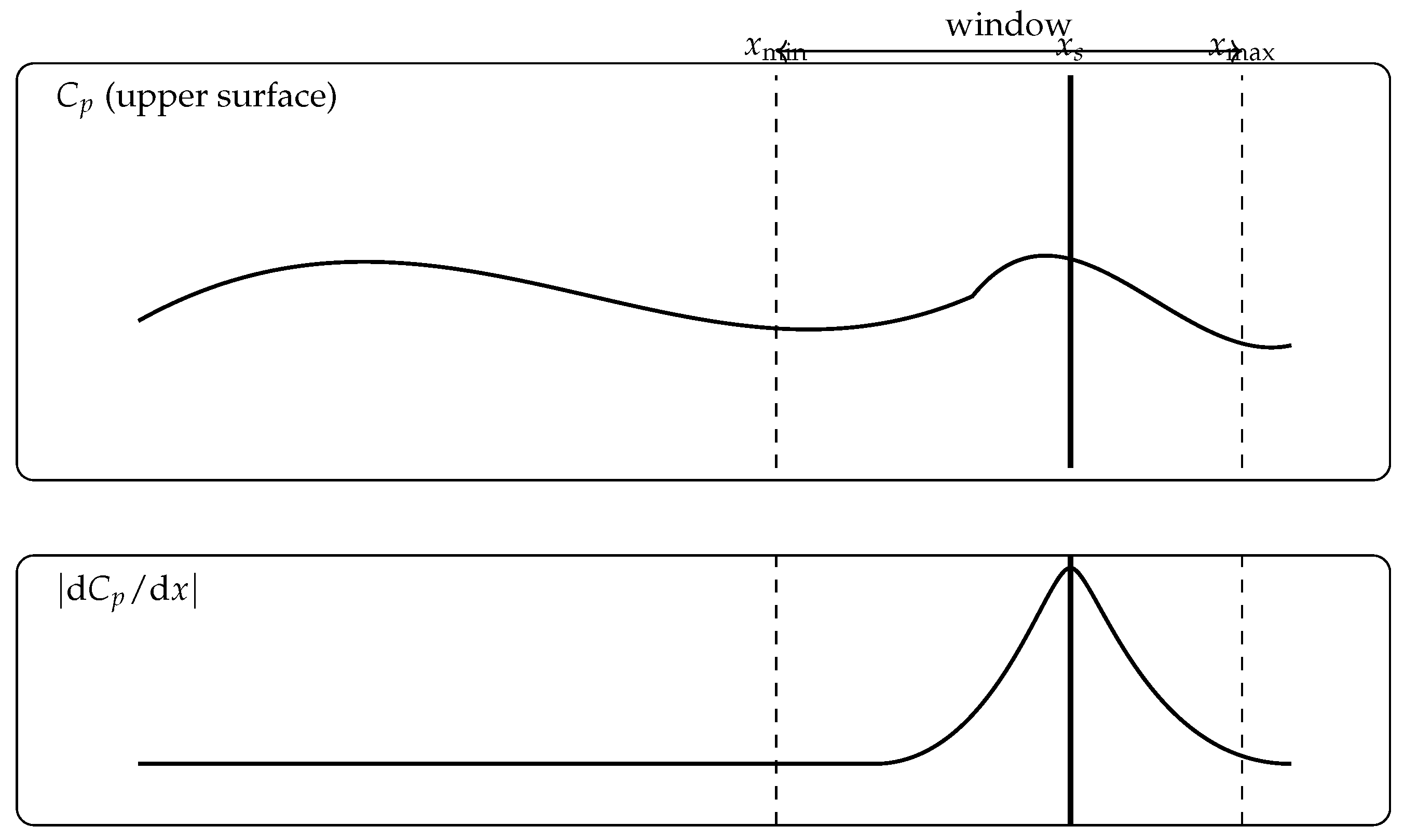
2.6.3. Define Shock Score Within a Chordwise Window

We compute the magnitude of the chordwise pressure gradient on a uniform grid $x\in [0,1]$ with spacing $\Delta x=1/(W-1)$. Using a standard centered difference for interior points,

$${\left.{\displaystyle \frac{d{C}_p}{dx}}\right|}_i\approx {\displaystyle \frac{C_{p,i+1}-C_{p,i-1}}{2\Delta x}},$$

(11)

we restrict attention to a chordwise window $x\in [x_{min},x_{max}]$ to avoid spurious leading-/trailing-edge gradients. The shock score is defined as the mean of the top fraction $p_{\mathrm{top}}$ of $\left|d{C}_p/dx\right|$ values inside this window:

$$S={\displaystyle \frac{1}{\left|T\right|}}\sum _{i\in T}\left|{\left.{\displaystyle \frac{d{C}_p}{dx}}\right|}_i\right|,$$

(12)

In implementation, the chordwise window $[x_{min},x_{max}]$ is mapped to index bounds $i_0=\lfloor \mathrm{clip}(x_{min},0,1)(W-1)\rfloor$ and $i_1=\lfloor \mathrm{clip}(x_{max},0,1)(W-1)\rfloor$ on the uniform grid. If the window becomes too short (e.g., $i_1\le i_0+5$), the full domain $[0,1]$ is used as a deterministic fallback. To suppress spurious leading-/trailing-edge peaks, the peak search excludes a small index margin near the window boundaries: we define $m=max\{3,\lfloor 0.01n\rfloor \}$ where n is the number of samples in the final window, and search the maximum-gradient index only on $[i_0+m,i_1-m]$ when $2m<n$. The shock location $x_s$ is taken at the maximum-gradient index inside the (possibly margin-trimmed) window; in the event of equal maxima (multi-peak ties), we break ties deterministically by selecting the smallest index (most-upstream location) to ensure reproducibility. Finally, as a robustness check against residual boundary artifacts, if the selected peak index falls within the excluded margin region (which can only occur when $2m\ge n$), the algorithm reverts to the full-window argmax with the same deterministic tie-breaking.

To quantify shock strength, we compute a code-consistent pressure jump using symmetric chordwise neighborhoods around the detected shock index. Let $i_p$ denote the peak-gradient index and define a window half-width $w=max(3,\lfloor 0.015W\rfloor )$. The upstream and downstream means are ${\overline{C}}_{p,\mathrm{L}}=\mathrm{mean}{\left\{C_{p,i}\right\}}_{i=i_p-w}^{i_p-1}$ and ${\overline{C}}_{p,\mathrm{R}}=\mathrm{mean}{\left\{C_{p,i}\right\}}_{i=i_p}^{i_p+w-1}$, respectively, and the shock jump magnitude is

$$\Delta C_p=\left|{\overline{C}}_{p,\mathrm{R}}-{\overline{C}}_{p,\mathrm{L}}\right|.$$

(13)

The corresponding extraction window and peak-detection rule are illustrated in Figure 5.

2.7. Optimization Formulation and Soft-Penalty Feasibility

We solve a scalarized optimization problem using differential evolution (DE) to reduce sensitivity to local minima and to handle the nonconvex, shock-sensitive response surface. Let a denote the CST vector and let the surrogate-predicted quantities entering Equation (14) be those defined above. The target lift coefficient is $C_L^{*}$; $R\left(a\right)$ is a small quadratic regularizer that discourages excessive deviation from the baseline parameters; and $P_{\mathrm{thick}}\left(a\right)$ penalizes thickness feasibility violation.

$$J\left(\mathbf{a}\right)=w_{cd}{\widehat{C}}_D\left(\mathbf{a}\right)+w_{\mathrm{shock}}\widehat{S}\left(\mathbf{a}\right)+w_{cl}{\left({\widehat{C}}_L\left(\mathbf{a}\right)-C_L^{*}\right)}^2+w_{\mathrm{reg}}R\left(\mathbf{a}\right)+w_{\mathrm{thick}}{P}_{\mathrm{thick}}\left(\mathbf{a}\right),$$

(14)

Under this formulation, drag reduction remains the primary optimization objective, while lift targeting and thickness preservation are enforced through soft penalties. The shock term introduces a physics-based preference for weaker transonic pressure jumps. Accordingly, the problem is interpreted as drag-oriented, lift-targeted aerodynamic shape optimization with thickness feasibility control, rather than strict target pressure inverse design.

Selected candidates from different $w_{\mathrm{shock}}$ settings are then re-evaluated using CFD, forming a closed-loop verification that quantifies surrogate bias and confirms true aerodynamic gains. In the revised manuscript, rather than displaying the full dense sweep directly, a representative subset of weight levels is retained to construct a compact Pareto-like trade-off view that more clearly reveals the role of the scalarization weight in the drag–shock compromise.

A recurring challenge in surrogate-based ASO is that DE can exploit low-sensitivity regions of the surrogate and generate mathematically favorable yet physically unrealistic airfoils, especially extremely thin shapes that appear to reduce drag. Such solutions are undesirable for practical aircraft design and can also degrade robustness in downstream CFD verification. To prevent this failure mode, we explicitly impose a baseline-relative chordwise thickness lower-bound condition through a soft-penalty feasibility term.

2.7.1. Baseline-Relative Thickness Lower-Bound Condition (Soft-Penalty Feasibility)

Let $t(a,x)$ denote the chordwise thickness distribution of a candidate airfoil, computed from the CST geometry as the distance between upper and lower surfaces. Let $t_0\left(x\right)$ be the baseline (RAE2822) thickness distribution evaluated on the same chordwise grid ${\left\{x_j\right\}}_{j=1}^{N_x}$. We enforce a baseline-relative lower bound

$$t(a,x_j)\ge \eta t_0\left(x_j\right),j=1,\dots ,N_x,$$

(15)

where $0<\eta \le 1$ is a user-specified feasibility factor (implementation parameter thick_min_frac). This feasibility condition is imposed via a soft penalty

$$P_{\mathrm{thick}}\left(a\right)={\displaystyle \frac{1}{N_x}}\sum _{j=1}^{N_x}{\left[max\left(0,\eta -{\displaystyle \frac{t(a,x_j)}{max(t_0\left(x_j\right),ϵ)}}\right)\right]}^2,$$

(16)

with a small $ϵ$ to avoid division by zero. For reporting and feasibility auditing, we additionally record

$$t_{min\_ratio}\left(a\right)=\underset{j}{min}{\displaystyle \frac{t(a,x_j)}{max(t_0\left(x_j\right),ϵ)}}.$$

(17)

For feasibility auditing in sweep experiments, we report (i) the thickness feasibility factor $\eta$ (implementation parameter thick_min_frac), (ii) the lift-tolerance ${ϵ}_{CL}$ used to judge lift-target compliance, and (iii) the sweep-level compliance rate defined as

$${\mathrm{CR}}_{CL}={\displaystyle \frac{1}{N_{\mathrm{sweep}}}}\sum _{r=1}^{N_{\mathrm{sweep}}}\mathbb{I}\left(\left|C_{L,r}^{\mathrm{Pred}}-C_L^{*}\right|\le {ϵ}_{CL}\right).$$

To interpret optimization behavior under scalarization, we additionally report the effective contribution ratios of each objective term (drag, shock, lift-targeting, regularization, thickness penalty) for the highlighted design and summarized statistics over sweep runs.

2.7.2. DE Settings

Population size $N_p$, maximum generations $G_{max}$, and the random seed are controlled by de_popsize, de_maxiter, and de_seed, respectively (with de_seed = 0 in this work). DE is implemented using scipy.optimize.differential_evolution. The final solution can optionally be refined by the built-in local search (setting polish=True).

2.8. Robust Closed-Loop CFD Verification and Fallback Strategies

To validate surrogate-proposed optima and close the engineering loop, we employ a fully automated CFD verification workflow based on SU2 Reynolds-averaged Navier–Stokes (RANS) simulations. Once the optimizer outputs the final geometry, the pipeline automatically performs geometry export, viscous mesh generation, SU2 execution, and post-processing of $(C_L,C_D)$ and shock-related metrics. This automation eliminates manual intervention in routine verification while preserving strict consistency of operating conditions between optimization and high-fidelity assessment.

In practice, heuristic optimizers can occasionally produce geometries that are numerically difficult for transonic CFD, due to local curvature extremes, near-singular thickness distributions, or mesh-quality degradation. To prevent such cases from breaking the pipeline, we implement a two-tier fallback mechanism.

Tier 1: Solver parameter relaxation. If divergence is detected from SU2 residual history, the workflow automatically restarts the case with progressively reduced Courant–Friedrichs–Lewy (CFL) numbers and disables multigrid acceleration. In particular, the CFL value is decreased through a predefined schedule (e.g., from 10.0 down to 0.2), and multigrid is switched off to prioritize numerical stability over convergence speed.

Tier 2: Progressive geometry blending. If the solver still diverges after Tier 1, the failed geometry is gradually blended toward the baseline RAE2822 in fixed 5% increments:

$${\mathbf{CST}}_{\mathrm{blend}}=(1-\alpha ){\mathbf{CST}}_{\mathrm{opt}}+\alpha {\mathbf{CST}}_{\mathrm{base}},\alpha \in \{0.05,0.10,\dots ,1.00\}.$$

(18)

For each updated $\alpha$, the pipeline re-meshes and re-runs SU2 until convergence is achieved. The first converged candidate is accepted as the CFD-verifiable output for that optimization run.

This staged degradation strategy significantly improves end-to-end robustness: even when the nominal optimum is not directly solvable, the framework still returns a reliable and verifiable improved design without human tuning, thereby bridging theoretical optimization and practical engineering deployment.

Measured robustness statistics. To avoid conflating solver robustness interventions with aerodynamic performance claims, we distinguish (a) directly converged optimized shapes (Tier-0/Tier-1 only) from (b) blended fallback shapes (Tier-2 invoked). Across sweep runs, we report the fallback frequency (fraction of cases requiring Tier-2) and the distribution of the accepted blending factor $\alpha$ (e.g., median and interquartile range), so robustness gains are quantified rather than only described. A compact definition of these robustness statistics is provided in

Table 4. Definitions of closed-loop CFD robustness statistics reported over sweep runs.

Item	Definition	Notes
Tier-2 usage rate	$N_{\text{Tier2}}/N_{\mathrm{sweep}}$	fraction of runs requiring geometry blending
Accepted $\alpha$ (median [P25,P75])	summary over accepted $\alpha$ values in Tier-2 cases	for Tier-2 cases only
Directly converged runs	$N_{\text{Tier0}}+N_{\text{Tier1}}$	Tier-0/Tier-1 only

, and the corresponding numerical values can be generated from the sweep logs using the released post-processing scripts.

3. Results

Numerical reporting convention. Reported values are rounded to a level appropriate for CFD-based engineering comparison. In this paper, $C_L$ and $C_m$ are reported to four decimal places, $C_D$ to five decimal places, $L/D$ to two decimal places, and $(x_s,\Delta C_p)$ to three decimal places unless additional digits are necessary to avoid ambiguity. Percentage changes are reported to one decimal place in the main baseline-vs-selected comparison and to two decimal places in the supplementary multi-incidence comparison when finer separation is needed. This convention is intended to support consistent within-study comparison and should not be interpreted as implying physical certainty beyond the fidelity of the underlying simulations.

3.1. Surrogate Training Performance

On the held-out test set ($N_{\mathrm{test}}=500$), the proposed multi-task surrogate achieves MAE/RMSE values of 0.00474/0.00602 for $C_L$ and $4.66\times {10}^{-4}/6.33\times {10}^{-4}$ for $C_D$. For the recovered $C_p$ curves, the upper- and lower-surface errors are MAE/RMSE = 0.00345/0.00871 and $0.00170/0.01953$, respectively. More importantly for the present optimization task, the shock-related quantities extracted from the recovered upper-surface $C_p$ curve yield MAE/RMSE values of 0.00201/0.01598 for the shock location indicator $x_s$ and 0.00200/0.00336 for the shock-jump metric $\Delta C_p$, as summarized in

Table 5. Quantitative accuracy metrics of the surrogate model on the held-out test set ($N_{\mathrm{test}}=500$).

Metric	MAE	RMSE
$C_L$	0.00474	0.00602
$C_D$	4.66 $\times {10}^{-4}$	6.33 $\times {10}^{-4}$
$C_{p,\mathrm{upper}}$ (curve)	0.00345	0.00871
$C_{p,\mathrm{lower}}$ (curve)	0.00170	0.01953
Shock location $x_s$	0.00201	0.01598
Shock jump $\Delta C_p$	0.00200	0.00336

.

These statistics are reported here not only as standard predictive-accuracy metrics, but also as an explicit uncertainty analysis for the shock-related surrogate outputs used inside the optimization loop. In the present framework, the optimizer does not act on a visually interpreted pressure curve; rather, it acts on deterministic shock descriptors extracted from the recovered pressure representation. Therefore, the predictive reliability of $(x_s,\Delta C_p)$ is directly relevant to the credibility of the optimization process. The test-set error levels indicate that the surrogate remains sufficiently accurate for engineering-oriented trend assessment of shock behavior, while also revealing a clear asymmetry between the two shock-related quantities: $\Delta C_p$ is predicted more tightly and consistently than the absolute shock location $x_s$.

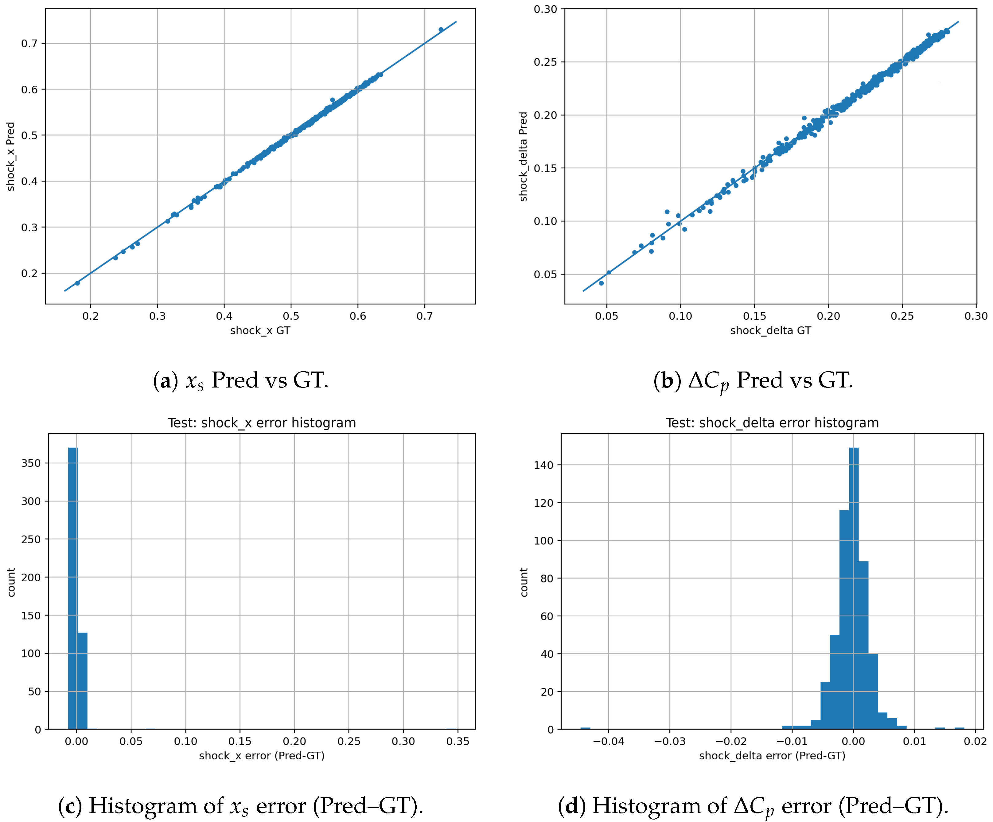
Figure 6 further visualizes the prediction quality and error distribution of these two quantities. The scatter plots show that both $x_s$ and $\Delta C_p$ follow the one-to-one trend closely for most samples, whereas the error histograms remain concentrated around zero with limited tails. At the same time, the larger spread observed for $x_s$ is physically reasonable in transonic pressure curves, because a shock location detector may become more sensitive when the local pressure gradient is broad, weak, or contains multiple nearby extrema. By contrast, the jump magnitude $\Delta C_p$ is a more aggregated descriptor of the local compression intensity and is therefore less sensitive to small positional ambiguity.

To facilitate interpretation, the correspondence between objective terms, reported metrics, and the main discussion/conclusion claims is summarized in

Table 6. Crosswalk from objective terms to reported metrics and supported claims.

Objective Term	Reported Metric(s)	Supported Claim in Section 4 and Section 5
$w_{cd}{C}_D$	$C_D$ (Pred/CFD), $\Delta C_D$	Drag reduction is preserved under CFD verification
$w_{\mathrm{shock}}S$	S, $\Delta C_p$, $x_s$	Shock intensity is mitigated; S– $\Delta C_p$ linkage is evidenced
$w_{cl}{(C_L-C_L^{*})}^2$	$|C_L-C_L^{*}|$, compliance rate	Lift-targeted soft-penalty feasibility across sweep cases
$w_{reg}R\left(a\right)$	$R\left(a\right)$/parameter distance	Avoids extreme CST deviations and stabilizes optimization
$w_{thick}{P}_{\mathrm{thick}}$	$t_{min\_ratio}$, $P_{\mathrm{thick}}$	Prevents unrealistic thin designs; enforces feasibility

.

From the standpoint of optimization sensitivity, the results in Table 5 and Figure 6 imply that the shock-related surrogate outputs should not be interpreted uniformly. The relatively tighter distribution of $\Delta C_p$ errors indicates that shock-intensity variation is captured more robustly than exact shock position. This distinction is important because the present optimizer uses shock-related quantities inside a scalarized objective. In consequence, the revised manuscript interprets $x_s$ primarily as a trend-level descriptor of the compression pattern, whereas $\Delta C_p$ is treated as the more stable engineering indicator of shock mitigation. The final design conclusions are therefore based on surrogate-guided search combined with closed-loop CFD verification, rather than on surrogate-predicted shock location alone.

3.2. Shock-Aware Optimization Results (Surrogate-Based)

For the selected $w_{\mathrm{shock}}=0.45$ case under the lift-targeted setting ($C_L^{*}=0.746$), the surrogate identifies a drag-reduced design with the following predicted characteristics:

• $C_{L,\mathrm{Pred}}=0.7271$ (vs. baseline: $-2.5\%$),
• $C_{D,\mathrm{Pred}}=0.01217$ (vs. baseline: $-16.8\%$),
• $x_{s,\mathrm{Pred}}=0.740$ and $\Delta C_{p,\mathrm{Pred}}=0.026$ (vs. baseline: $-89.1\%$ for $\Delta C_p$),
• ${(L/D)}_{\mathrm{Pred}}=59.74$.

The highlighted design ($w_{\mathrm{shock}}=0.45$) is summarized not only by $(C_L,C_D,x_s,\Delta C_p)$ but also by a fully traceable objective decomposition. All terms are exported by the optimization script in opt/best_info.json and are reported in

Table 7. Objective-term breakdown for the highlighted design ($w_{\mathrm{shock}}=0.45$).

Term	Definition	Value
Drag term	$w_{cd}{C}_D$	$0.009939$
Shock term	$w_{\mathrm{shock}}S$	$0.778565$
Lift targeting	$w_{cl}{(C_L-C_L^{*})}^2$	$0.050368$
Regularization	$w_{reg}R\left(a\right)$	$6.41\times {10}^{-6}$
Thickness penalty	$w_{thick}{P}_{\mathrm{thick}}\left(a\right)$	$0.037993$
Total	$J\left(a\right)$	$0.876872$

.

3.3. Drag–Shock Trade-Off and Representative Pareto-like Analysis

A key advantage of the proposed framework is that the shock penalty weight $w_{\mathrm{shock}}$ acts as a physically interpretable control parameter that explicitly regulates the balance between drag reduction and shock mitigation. In many transonic optimizations, the influence of shock control remains implicit in the final drag-oriented objective. By contrast, the present formulation retains an explicit shock-related penalty term, allowing the effect of different scalarization choices to be examined directly.

To address the reviewer’s concern regarding manually tuned scalarization weights, a parametric sweep of $w_{\mathrm{shock}}$ was performed. For each prescribed weight, an independent optimization was carried out using the differential evolution (DE) optimizer, and the resulting design was subsequently validated through closed-loop CFD simulations. Because each run still corresponds to a scalarized single-objective optimization, the resulting solution set is described here as a Pareto-like trade-off rather than a strict mathematical Pareto front. Nevertheless, this analysis provides a transparent and practically meaningful view of how the manually specified shock penalty shifts the final design toward different drag–shock compromises.

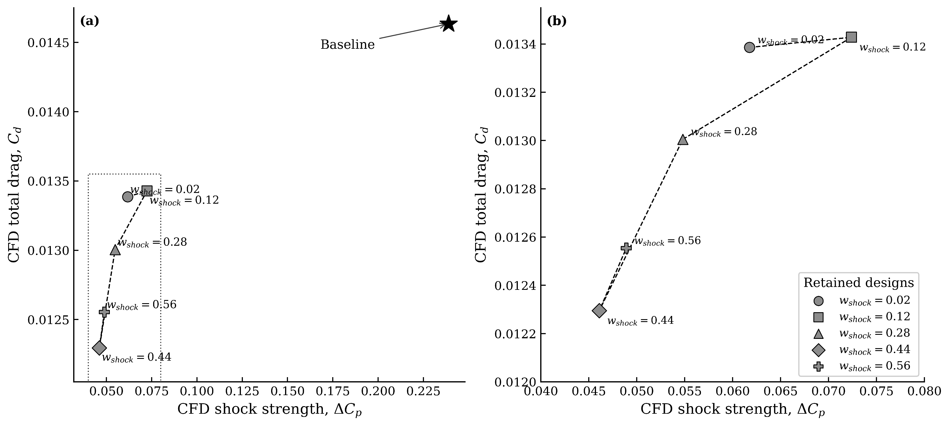
For clarity, instead of showing the entire dense sweep, five representative weight levels were retained,

$$w_{\mathrm{shock}}=0,0.10,0.30,0.45,0.55,$$

which span the design spectrum from weak to strong shock penalization. This reduced representation is sufficient to reveal the underlying trade-off trend while keeping the figure concise and easy to interpret.

As shown in Figure 7, increasing the shock penalty weight systematically shifts the optimized solutions away from the baseline and toward a lower-shock regime. When $w_{\mathrm{shock}}$ is small ($w_{\mathrm{shock}}=0$ or $0.10$), the optimization remains relatively drag-oriented and the resulting shock suppression is limited. As the shock penalty increases, the solutions move toward weaker shock intensity and improved pressure recovery characteristics. This trend confirms that the final design behavior is not governed by an arbitrary single weight choice, but by a systematic and interpretable drag–shock compromise.

Table 8. Representative retained solutions from the $w_{\mathrm{shock}}$ sweep.

${\mathit{w}}_{\mathbf{shock}}$	Pred_${\mathit{C}}_{\mathit{L}}$	Pred_${\mathit{C}}_{\mathit{D}}$	CFD_${\mathit{C}}_{\mathit{L}}$	CFD_${\mathit{C}}_{\mathit{D}}$	Pred_${\mathit{C}}_{\mathit{D}}$/Init (%)	CFD_${\mathit{C}}_{\mathit{D}}$/Init (%)
0	0.7794	0.0136	0.7917	0.0134	93.1099	91.5169
0.10	0.7644	0.0132	0.7670	0.0131	90.3317	89.3996
0.30	0.7418	0.0126	0.7473	0.0129	86.4384	88.3507
0.45	0.7271	0.0122	0.7313	0.0123	83.1900	84.0270
0.55	0.7165	0.0121	0.7209	0.0122	82.7237	83.1868

lists the aerodynamic coefficients of the retained representative designs. The low-weight case ($w_{\mathrm{shock}}=0$) provides only limited overall improvement relative to the baseline, indicating that weak shock penalization is insufficient to fully exploit the shock-aware design space. As the shock penalty increases to intermediate levels, both drag reduction and shock alleviation become more pronounced. In particular, the retained case at $w_{\mathrm{shock}}=0.45$ provides a balanced compromise between low drag and effective shock suppression and is therefore selected as the main representative design in the present study. The higher-weight case ($w_{\mathrm{shock}}=0.55$) further emphasizes shock mitigation while maintaining a comparable drag level, illustrating the controllability of the scalarized optimization framework.

Overall, the representative Pareto-like analysis demonstrates that the final optimized design should not be interpreted as the result of an arbitrary scalarization choice. Instead, it is selected from a CFD-verified family of solutions spanning different shock penalty levels, and thus represents a deliberate compromise between drag reduction and shock mitigation. This considerably improves the transparency of the optimization framework and directly addresses the concern regarding manually tuned scalarization weights.

3.4. Closed-Loop CFD Verification

We perform CFD verification on the selected design from Section 3.2 ($w_{\mathrm{shock}}=0.45$):

• Baseline CFD (RAE2822 reference): $C_{L,\mathrm{CFD},\mathrm{base}}=0.7461$, $C_{D,\mathrm{CFD},\mathrm{base}}=0.01463$, $x_{s,\mathrm{CFD},\mathrm{base}}=0.542$, and $\Delta C_{p,\mathrm{CFD},\mathrm{base}}=0.239$.
• Optimized CFD: $C_{L,\mathrm{CFD},\mathrm{opt}}=0.7313$, $C_{D,\mathrm{CFD},\mathrm{opt}}=0.01229$, $x_{s,\mathrm{CFD},\mathrm{opt}}=0.479$, and $\Delta C_{p,\mathrm{CFD},\mathrm{opt}}=0.046$.
• CFD-verified improvements: $\Delta C_{D,\mathrm{CFD}}=-0.00234$ ($-16.0\%$ relative to baseline), $\Delta {(\Delta C_p)}_{\mathrm{CFD}}=-0.193$ ($-80.7\%$ relative to baseline), $\Delta x_{s,\mathrm{CFD}}=-0.063$, and ${(L/D)}_{\mathrm{CFD}}$ improves from 51.00 to 59.49.

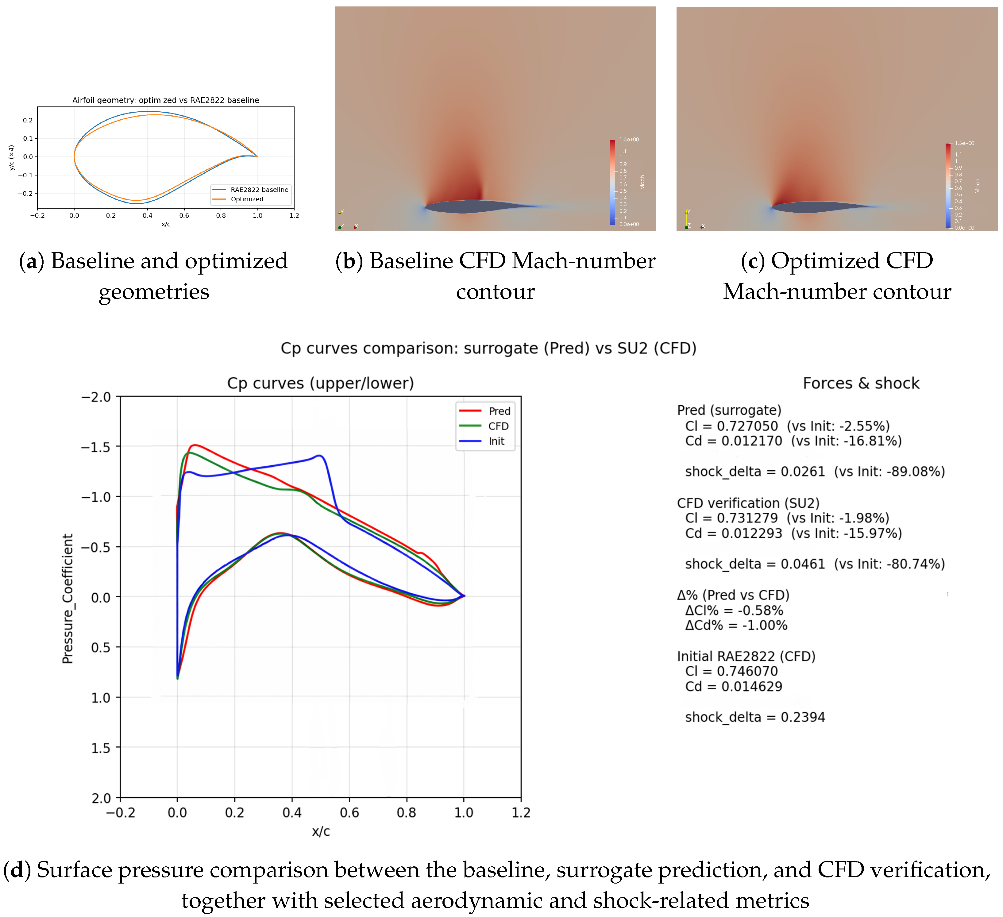
Beyond the scalar reductions in drag and shock intensity, it is necessary to examine whether the optimized state remains aerodynamically meaningful in the context of transonic airfoil design. Figure 8 therefore presents the selected design using complementary views of geometry, CFD flow field, and surface pressure distribution. The baseline and optimized geometries are first compared directly, followed by the corresponding CFD Mach number contours under the same operating condition and color scale. The pressure distribution comparison then links the geometric modification to the observed redistribution of the upper-surface compression–recovery pattern and the weakening of the shock jump.

The results in Figure 8 support the interpretation that the optimized airfoil constitutes a physically meaningful transonic redesign rather than a geometry favored only by the surrogate. At the same time, the discrepancy between surrogate-predicted and CFD-verified $x_s$ should be interpreted together with the test-set uncertainty analysis reported earlier. Specifically, the held-out error statistics and the scatter/histogram distributions in Figure 6 indicate that the present surrogate is more reliable for capturing shock intensity variation than for prescribing an exact shock location. For this reason, the revised manuscript treats the agreement in $\Delta C_p$ reduction and drag reduction under CFD verification as stronger evidence of design success, while interpreting $x_s$ primarily as a trend-level descriptor of the upper-surface compression pattern. Likewise, the local plateau/wiggle observed on the optimized upper-surface $C_p$ curve is interpreted here as a redistributed compression–recovery pattern, not as direct evidence of flow separation, because no dedicated separation diagnostic is included in the present study. The pitching moment coefficient is reported for the CFD-evaluated cases to assess whether the drag reduction is accompanied by a pitching moment penalty, whereas the present surrogate is trained only to predict $(C_L,C_D)$ and the pressure distribution representation.

A direct comparison of the predicted and CFD-verified aerodynamic/shock metrics for the selected design is provided in

Table 9. Comparison of aerodynamic coefficients, pitching moment, and shock indicators for the selected design ($w_{\mathrm{shock}}=0.45$).

Airfoil	Source	${\mathit{C}}_{\mathit{L}}$	${\mathit{C}}_{\mathit{D}}$	${\mathit{C}}_{\mathit{m}}$	$\mathit{L}/\mathit{D}$	${\mathit{x}}_{\mathit{s}}$	$\mathbf{\Delta }{\mathit{C}}_{\mathit{p}}$
Baseline (RAE2822)	CFD	0.7461	0.01463	0.0898	51.00	0.542	0.239
Optimized ($w_{\mathrm{shock}}=0.45$)	Pred	0.7271	0.01217	—	59.74	0.740	0.026
Optimized ($w_{\mathrm{shock}}=0.45$)	CFD	0.7313	0.01229	0.0939	59.49	0.479	0.046

.

The pitching moment coefficient is reported only for the CFD-evaluated cases because the present surrogate is trained to predict $(C_L,C_D)$ and the pressure distribution representation, rather than $C_m$ directly.

3.5. Additional CFD Validation Under Nearby Off-Design Conditions

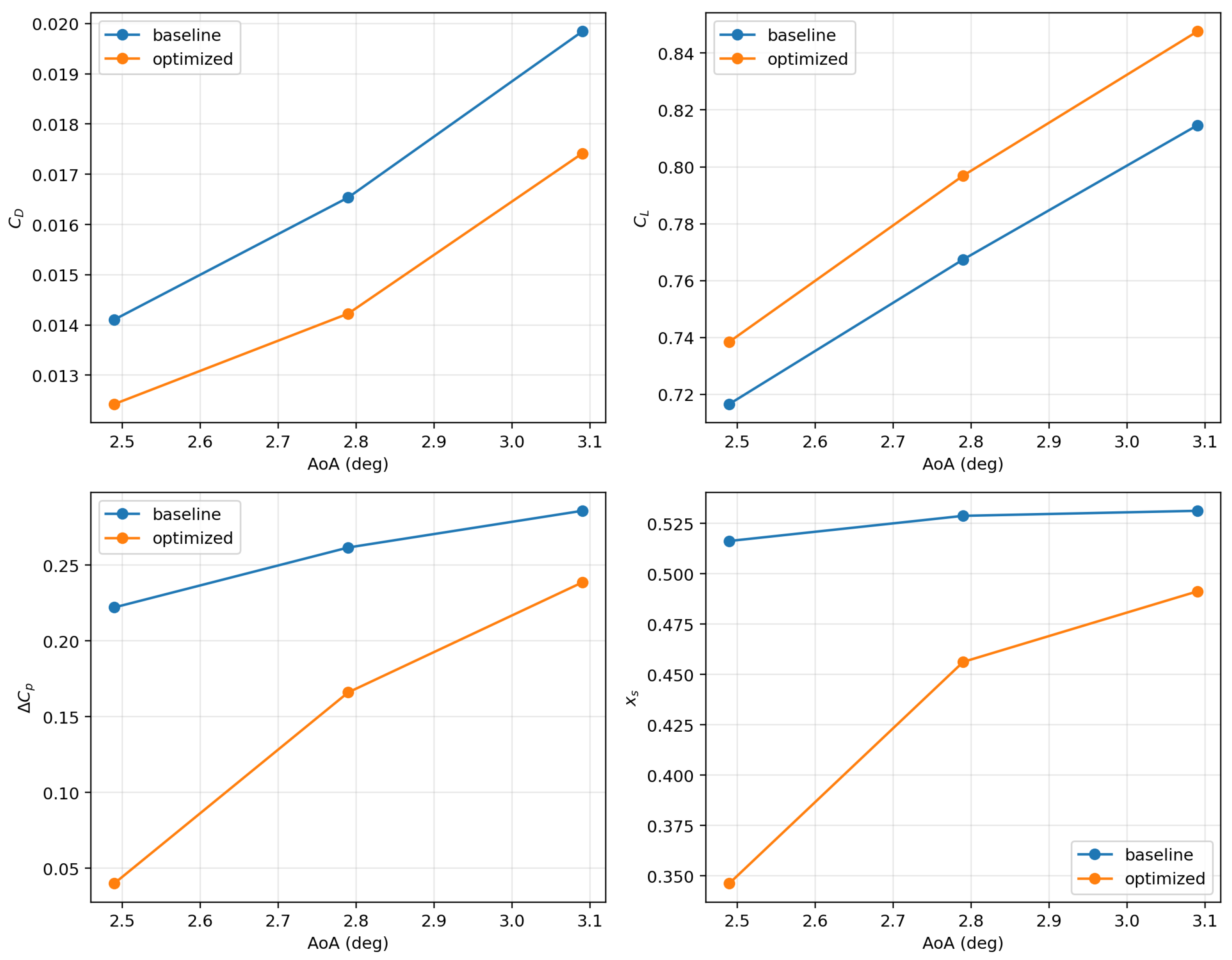
To further examine whether the selected optimized airfoil remains effective beyond the nominal design incidence, additional closed-loop CFD validations were performed under three nearby fixed-incidence conditions, namely ${\alpha }_0-0.3^{\circ }$, ${\alpha }_0$, and ${\alpha }_0+0.3^{\circ }$. In the present study, these additional validations were conducted at fixed incidences rather than under re-trimmed equal-lift conditions, so the purpose of this analysis is to assess nearby off-design robustness in a controlled sense, rather than to establish a fully trimmed multi-condition performance envelope.

Table 10. Closed-loop CFD comparison under three nearby AoA conditions.

Geometry	AoA (Deg)	${\mathit{C}}_{\mathit{L}}$	${\mathit{C}}_{\mathit{D}}$	${\mathit{x}}_{\mathit{s}}$	$\mathbf{\Delta }{\mathit{C}}_{\mathit{p}}$	$\mathbf{\Delta }{\mathit{C}}_{\mathit{D}}$ vs. Baseline (%)
baseline	2.490	0.716582	0.014105	0.5162	0.2220	–
optimized	2.490	0.738461	0.012423	0.3463	0.0400	−11.92
baseline	2.790	0.767441	0.016538	0.5288	0.2615	–
optimized	2.790	0.796923	0.014226	0.4563	0.1660	−13.98
baseline	3.090	0.814592	0.019844	0.5312	0.2858	–
optimized	3.090	0.847590	0.017415	0.4912	0.2385	−12.24

summarizes the CFD results for both the baseline and optimized airfoils. At all three incidences, the optimized airfoil maintains a lower drag coefficient than the baseline, with drag reductions of 11.92%, 13.98%, and 12.24%, respectively. At the same time, the shock jump metric $\Delta C_p$ is also reduced at all three incidences, although the magnitude of shock mitigation decreases as the angle of attack increases. Specifically, the reduction in $\Delta C_p$ is 81.98% at $\alpha =2.{49}^{\circ }$, 36.52% at $\alpha =2.{79}^{\circ }$, and 16.55% at $\alpha =3.{09}^{\circ }$. This indicates that the optimized geometry preserves the overall tendency toward weaker compression and lower drag under nearby off-design conditions, while the shock suppression advantage becomes progressively less pronounced as the incidence moves upward from the nominal operating point.

Figure 9 provides a compact comparison of the main aerodynamic and shock-related quantities across the three incidences. The baseline airfoil exhibits the expected increase in $C_L$, $C_D$, and $\Delta C_p$ as the angle of attack increases, while the optimized airfoil follows the same overall trend but remains consistently below the baseline in drag and generally below it in shock intensity. The gap in $\Delta C_p$ between the two geometries is especially large at the lower incidence and becomes smaller at the higher incidence, which is consistent with the interpretation that the present optimized geometry is most effective near the nominal design neighborhood rather than uniformly across a broad range of incidences.

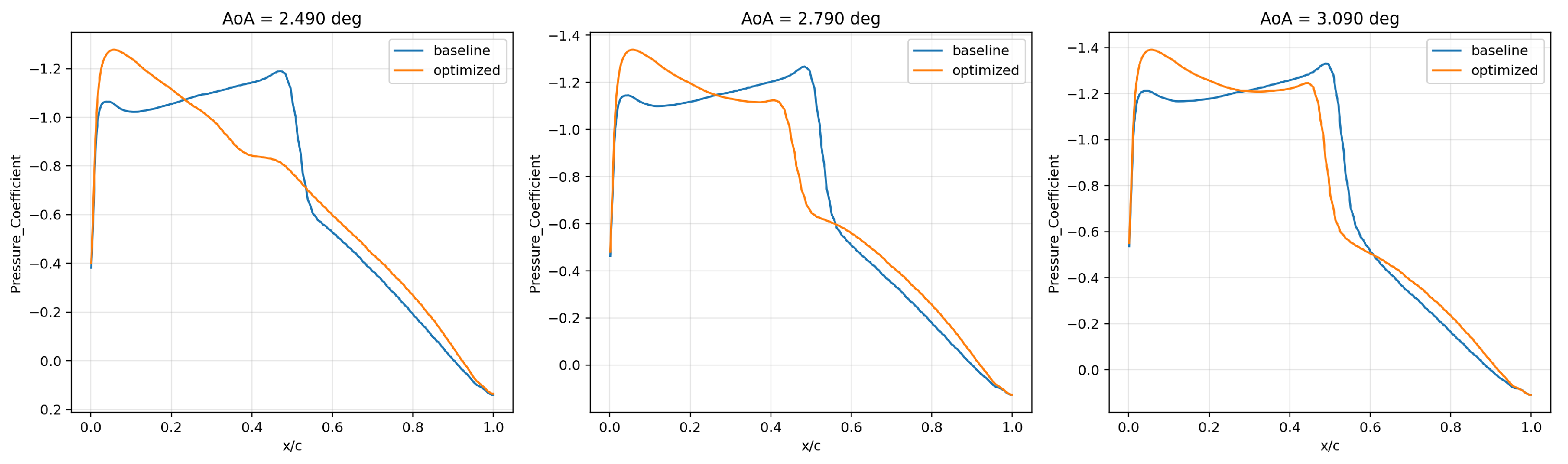
The upper-surface pressure distributions are compared in Figure 10. At $\alpha =2.{49}^{\circ }$, the optimized airfoil shows a much weaker compression pattern than the baseline, and the identified shock jump becomes very small. At $\alpha =2.{79}^{\circ }$, the optimized airfoil still exhibits a visibly weaker shock than the baseline, but the difference is less extreme than that at the lower incidence. At $\alpha =3.{09}^{\circ }$, the optimized airfoil continues to show a favorable trend, although the local compression pattern becomes stronger and the shock mitigation margin is further reduced. These curve-level observations are consistent with the quantitative results in Table 10: the drag advantage remains stable across the three tested incidences, whereas the shock-intensity advantage gradually diminishes as AoA increases.

Overall, these additional multi-incidence CFD results strengthen the interpretation that the proposed framework does not merely produce a single-point numerical improvement. Instead, the selected optimized geometry retains lower drag and generally weaker shock intensity within a nearby off-design incidence range around the nominal operating condition. At the same time, the present results also show that this robustness is local rather than uniform: as the incidence increases, the shock mitigation benefit gradually weakens, even though the drag benefit remains clearly observable.

4. Discussion

The combined geometry, flow-field, and pressure distribution evidence indicates that the selected design constitutes a physically meaningful transonic redesign. Relative to the baseline airfoil, it weakens the upper-surface shock, reduces drag, and preserves a lift level close to the target operating condition. The additional reporting of $C_m$ is useful because it shows whether the drag benefit is obtained at the expense of a substantial pitching moment penalty. More importantly, the revised manuscript now makes explicit that the reliability of the shock-aware optimization loop should be evaluated at two different levels: the prediction uncertainty of the surrogate-derived shock metrics themselves, and the sensitivity of the final design interpretation to the corresponding prediction errors.

At the first level, the test-set statistics in Table 5 and the distributions in Figure 6 provide a direct uncertainty characterization for the shock-related surrogate outputs. These results show that both $x_s$ and $\Delta C_p$ can be recovered with good consistency on the held-out dataset, but also that the two quantities do not have the same robustness. The absolute shock location $x_s$ exhibits a visibly larger spread than the shock jump metric $\Delta C_p$, which is consistent with the underlying physics of transonic pressure curves: when the local pressure gradient becomes broad, weak, or contains multiple nearby extrema, a deterministic peak detector may shift its selected location even though the overall compression intensity remains similar. By contrast, $\Delta C_p$ is a more aggregated measure of the local jump strength and is therefore less sensitive to small positional ambiguity.

At the second level, the closed-loop CFD results clarify the design sensitivity implications of this error structure. The present workflow is more reliable for mitigating shock strength than for prescribing an exact shock position. In this sense, the shock location indicator should be interpreted primarily as a trend-level descriptor that helps characterize the compression pattern, whereas the stronger engineering conclusion of the present study lies in the consistent reduction in shock intensity and drag under closed-loop CFD verification. This is precisely why the revised manuscript no longer treats shock location agreement as a standalone success criterion. Instead, the final assessment of the selected design is based on the combined evidence of reduced $C_D$, reduced $\Delta C_p$, and physically interpretable pressure-redistribution behavior after CFD re-evaluation.

Two methodological implications follow from these results. First, the two-channel vSDF representation improves the stability of curve recovery and shock metric extraction in regions with steep pressure gradients. For the present optimization task, this property is more important than pixel-level image similarity, because the optimizer depends on preserving the local shock signature that governs wave drag trends. Second, closed-loop CFD verification remains essential. Even modest surrogate bias in $\Delta C_p$ or local ambiguity in $x_s$ can distort the apparent drag–shock trade-off obtained from surrogate-only sweeps and can therefore affect design ranking if CFD is not used as the final arbiter.

The thickness feasibility constraint is also essential from an engineering standpoint. Without it, the optimizer may exploit unrealistically thin sections that appear favorable to the surrogate but are of limited practical value and may be numerically fragile in downstream CFD. The adopted baseline-relative lower-bound formulation introduces a transparent feasibility parameter, $\eta$, and allows the resulting designs to be audited directly through tmin_ratio and $P_{\mathrm{thick}}$ together with the achieved drag reduction and shock mitigation metrics. The remaining surrogate-to-CFD discrepancies can be attributed to several sources, including limited training coverage near extreme geometries, rendering and curve extraction artifacts in the $C_p$ supervision, and CFD numerical sensitivity under shock-dominated conditions.

In addition, the supplementary fixed-incidence CFD validations under ${\alpha }_0\pm 0.3^{\circ }$ provide a more explicit view of the robustness boundary of the selected design. The optimized airfoil maintains lower drag than the baseline at all three tested incidences and also preserves a weaker shock signature in terms of $\Delta C_p$. However, the magnitude of shock mitigation decreases noticeably as AoA increases, indicating that the robustness demonstrated here should be interpreted as local off-design robustness around the nominal operating point rather than as uniform multi-condition superiority. This distinction is important because the present manuscript is intended to establish a controlled and auditable shock-aware optimization workflow, not to claim broad generality across all operating conditions.

5. Conclusions

This paper presents an engineering-oriented, closed-loop framework for drag-oriented, shock-aware scalarized optimization with soft-penalty feasibility for the RAE2822 transonic airfoil. A multi-task neural surrogate maps 16-dimensional CST parameters to a two-channel vSDF representation of upper/lower $C_p$ curves and aerodynamic coefficients, enabling deterministic recovery of shock descriptors for feature-aware optimization. The surrogate is embedded in a differential evolution optimizer under a lift-targeted formulation with a baseline-relative thickness penalty, and selected designs are verified by SU2 RANS.

An explicit uncertainty analysis on a held-out test set of 500 samples shows that the recovered shock-jump metric $\Delta C_p$ is predicted more tightly and consistently than the absolute shock location indicator $x_s$. Accordingly, the workflow is more reliable for controlling shock-intensity trends than for prescribing exact shock position. The final engineering conclusions are therefore drawn from surrogate-guided search combined with closed-loop CFD verification, rather than from surrogate-predicted shock location alone.

CFD verification confirms meaningful drag reduction together with substantial shock-intensity mitigation under the adopted lift-targeted, thickness-feasible formulation. Additional fixed-incidence validations at ${\alpha }_0-0.3^{\circ }$, ${\alpha }_0$, and ${\alpha }_0+0.3^{\circ }$ show that the selected design maintains lower drag and generally weaker shock intensity within a nearby off-design neighborhood. The drag reduction remains at approximately 12–14% across the three tested incidences, while the shock mitigation advantage weakens as AoA increases. These results indicate local off-design robustness, rather than uniform multi-condition superiority.

The main takeaways are:

• The two-channel vSDF representation provides a stable pressure surrogate that supports robust curve recovery and shock metric extraction, which are necessary for feature-aware optimization.
• A fixed, code-consistent procedure for extracting $(x_s,\Delta C_p)$ enables reproducible shock-aware objectives and consistent surrogate-to-CFD comparisons.
• The revised uncertainty analysis shows that $\Delta C_p$ is a more stable shock-related engineering descriptor than exact $x_s$, which clarifies how the surrogate outputs should be interpreted inside the optimization loop.
• By jointly predicting aerodynamic coefficients and reconstructing the pressure field, the surrogate supports rapid design search with a drag–shock composite objective and a thickness penalty, while closed-loop CFD verification provides the final basis for design acceptance.

Future work will extend the workflow to multiple operating conditions, multiple airfoil or wing geometries, and eventually three-dimensional configurations, while also investigating higher-fidelity or uncertainty-aware surrogates to further improve reliability in shock-dominated regimes. The representative Pareto-like analysis also improves interpretability of the scalarized setting by showing that the selected design is chosen from a CFD-verified drag–shock compromise family rather than from an isolated single-weight result.