


Abstract
High−Altitude wind is a critical factor affecting the recovery safety of reusable rockets, significantly altering aerodynamic loads, flight attitudes, and trajectories—especially during the aerodynamic deceleration phase (engine shutdown) of reentry, posing severe challenges to high-precision guidance and stable control. Currently, accurate advance prediction of landing site wind fields is difficult with poor real-time performance, necessitating a real-time estimation and prediction method independent of additional measurement equipment. This study addresses this gap by proposing a deep learning-based approach for wind field estimation and prediction, using directly measurable attitude angles and apparent acceleration deviations of the rocket as inputs to train a dedicated deep neural network. Furthermore, to solve the attitude control problem of Reusable Launch Vehicles (RLVs) during recovery, a non-recursive simplified high-order sliding mode control method with online wind disturbance compensation is designed to achieve finite-time convergence. First, a dynamic model for the attitude control of RLVs during recovery is established; second, based on homogeneity theory, a non-recursive simplified homogeneous high-order sliding mode controller is developed to realize finite-time tracking control during RLV recovery with uncertainties, effectively suppressing the chattering inherent in sliding mode control; finally, simulation results verify the effectiveness and engineering feasibility of the proposed method. The combined approach significantly reduces wind-induced disturbance torque and required control torque, enhancing the adaptability and control robustness of vertically recoverable rockets to wind fields.
1. Introduction
This study focuses on the autonomous load suppression and control of Reusable Launch Vehicles (RLVs) under sparse data conditions. To address the impact of High−Altitude wind on RLV recovery, a real-time wind field estimation and prediction method based on deep learning is first designed: only using directly measurable attitude angles and apparent acceleration deviations of the rocket as inputs, it identifies the current and future High−Altitude wind information around the rocket, enabling accurate online generation of wind profile programs. Furthermore, to meet the high-precision attitude control requirements during the rocket recovery phase, a non-recursive high-order sliding mode control strategy with finite-time convergence and online wind disturbance compensation is proposed, effectively solving problems such as aerodynamic load fluctuations and flight attitude instability caused by High−Altitude wind. Simulation results verify the effectiveness of the method, which not only improves the safety and reliability of rocket recovery but also simplifies the control algorithm and reduces the complexity of engineering implementation.
1.1. Technical Challenges of Online Wind Disturbance Compensation
High−Altitude wind disturbance is the primary interference source during the atmospheric reentry phase of RLVs, exerting a significant impact on flight states: if wind-induced loads exceed the rocket’s structural bearing limit, structural damage or even disintegration may occur, seriously threatening flight safety and recovery success rate.
Current engineering practices typically adopt offline trajectory wind compensation before launch to reduce aerodynamic loads during flight and improve safety; after launch, flight aerodynamic loads are evaluated to guide subsequent design iterations. However, limited by measurement technology, there is a lack of effective real-time High−Altitude wind measurement means during rocket flight, especially for landing site wind field prediction methods [1]. Thus, an online High−Altitude wind estimation and prediction method independent of additional measurement equipment is urgently needed.
The impact of High−Altitude wind is particularly prominent during the aerodynamic deceleration phase of RLV recovery: High−Altitude wind changes the airflow velocity, causing variations in the rocket’s relative airflow velocity, which in turn induces fluctuations in the Angle of Attack (AoA) and sideslip angle, generating additional aerodynamic forces and moments. Under the action of the rocket’s control system, the control torque generated by engine gimbaling or grid fin actuation must balance this additional aerodynamic moment, while the resultant force of the additional aerodynamic force and engine gimbal control force induces lateral and normal overloads.
1.2. Application of Deep Learning in Wind Field Estimation and Prediction
Deep learning excels at addressing problems characterized by strong data correlation yet complex modeling requirements. By adopting Deep Neural Networks (DNNs) as mathematical frameworks, it establishes input-output mapping relationships through training and parameter optimization, making it well-suited for tasks such as online numerical optimization, parameter identification, estimation fitting, and data trend prediction—challenges that are often cumbersome or infeasible with traditional modeling approaches. Recent advancements in deep learning have revolutionized aerospace engineering, with extensive applications in spacecraft guidance, dynamics, and control, demonstrating its potential as a game-changing technology in complex mission scenarios [1,2].
Recurrent Neural Networks (RNNs) and their enhanced variants, such as Long Short-Term Memory (LSTM) and Gated Recurrent Unit (GRU), are particularly proficient in processing time-series data. These models effectively mitigate the long-term dependency limitation of traditional RNNs, enabling widespread adoption in “sequence-to-sequence” or “sequence-to-point” parameter identification and feature extraction tasks within the aerospace domain [2]. For instance, Zhang et al. [3,4] and Kim et al. [5] leveraged LSTM networks as alternatives to conventional filters, using radar measurements to estimate trajectory information for missile tracking and launch point determination, thereby overcoming the significant tracking errors associated with complex system modeling. Similarly, Roux et al. [6] employed GRU to identify the guidance law of enemy interceptors based on motion data, achieving a substantial reduction in identification time compared to Kalman filter-based methods.
Another core application of LSTM lies in extracting trend features from existing data to enable reasonable extrapolation and future trend prediction. Beyond aerospace, this capability has been successfully applied to remaining useful life prediction for engineering systems [7], crystal diameter forecasting in silicon single crystal growth [8], and stock price prediction considering inter-asset correlations [9]. In the aerospace field, LSTM has delivered exceptional performance in hypersonic vehicle trajectory prediction, addressing the challenges posed by high maneuverability and the difficulty of establishing accurate physical models [10,11].
Estimating and predicting High−Altitude winds via rocket response data inherently constitutes a time-series processing problem, which aligns well with the strengths of deep learning methods. The key challenge lies in analyzing the response patterns of reusable launch vehicles (RLVs) under High−Altitude wind disturbances and the evolutionary characteristics of wind fields, as well as designing appropriate input-output configurations for deep neural networks. To address the High−Altitude wind disturbance during the atmospheric reentry phase of RLV recovery, this paper proposes a deep learning-based online High−Altitude wind estimation and prediction method. Utilizing only directly measurable attitude angles and apparent acceleration deviations as inputs, the method trains a deep neural network to achieve accurate estimation and prediction of High−Altitude wind speed and direction, eliminating the need for additional measurement equipment. In practical applications, this approach can significantly enhance the flight precision and safety of RLVs during recovery, ensure precise landing in predetermined recovery zones, and improve the reliability and economic efficiency of reusable rocket systems.
1.3. Research Status of Stabilization Control During Recovery
In recent decades, with the rapid development of aerospace technology toward hypersonic and reusable directions, the flight envelope of vehicles has continuously expanded. Their dynamic models exhibit strong nonlinearity, significant parameter perturbations, and complex external disturbances, placing higher demands on the robustness, rapidity, and control precision of stabilization control technology. Scholars worldwide have conducted extensive systematic research around this core demand, achieving fruitful results in robust control, active disturbance rejection control, and intelligent control, providing key technical support for the stabilization control of different types of vehicles. The specific research progress is summarized as follows:
In the field of robust control and active disturbance rejection control, aiming at the uncertainty and disturbance suppression problems of aircraft systems, scholars have proposed various innovative control strategies. Xu et al. [12] designed a robust controller, focusing on solving the disturbance sensitivity problem during aircraft reference command tracking. Simulation results show that the controller still maintains excellent robustness and tracking precision when facing parameter perturbations and external disturbances, effectively improving the system’s anti-disturbance capability; Han [13] focused on the decoupling control of nonlinear uncertain systems, combining feedback linearization technology with the Equivalent Input Disturbance (EID) method, successfully decomposing complex nonlinear systems into multiple canonical subsystems, and then designing Active Disturbance Rejection Control (ADRC) laws for each subsystem to achieve real-time compensation of internal and external disturbances and independent stable control of subsystems; Zhang [14] proposed a backstepping control method based on an Extended State Observer (ESO) for the dynamic performance requirements of aircraft attitude or trajectory tracking, using ESO to real-time estimate and compensate for unmodeled dynamics and external disturbances of the system, and combining the step-by-step recursive design idea of backstepping control to significantly improve the tracking response speed and steady-state precision of the controller, with simulation results verifying its effectiveness under complex working conditions; Liu [15] took air-breathing hypersonic vehicles as the research object, considering the strong coupling characteristics of their propulsion systems and aerodynamic properties, designed a disturbance-rejection dynamic inverse controller, and constructed a disturbance observer to online estimate the total system disturbance (including parameter perturbations, external disturbances, and unmodeled dynamics), effectively offsetting the impact of disturbances on control performance and ensuring stability during hypersonic flight; Fu [16] combined the strong robustness of invariant set sliding mode control with the disturbance estimation capability of a fast nonlinear disturbance observer, proposing a robust adaptive backstepping attitude control scheme, suppressing uncertain disturbances through the switching characteristics of sliding mode control, while optimizing the dynamic response process using backstepping control to achieve high-precision stable control of aircraft attitude.
In the field of intelligent control and constrained control, aiming at complex scenarios such as non-affine aircraft models and state constraints, relevant research has further expanded the scope of application of control methods. Bu [17] broke through the limitations of traditional affine models, taking the non-affine dynamic model of air-breathing hypersonic vehicles as the control object, designed a prescribed performance control strategy based on the nonlinear approximation capability of neural networks, and introduced a minimum learning parameter scheme to simplify the computational complexity of neural networks while ensuring control precision, solving the “curse of dimensionality” and parameter redundancy problems in non-affine system control; Wang [18] considered the safety hazard of ramjet flameout caused by excessive AoA during the flight of air-breathing hypersonic vehicles, proposing an adaptive backstepping control method with state constraints, ensuring that the AoA always remains within a safe range by introducing an AoA constraint mechanism in the control law design, while using an adaptive algorithm to online adjust control parameters, balancing system stability and flight safety; Zhao [19] approached from the perspective of data-driven control, combining a fixed-time neural disturbance observer with composite learning control, constructing a historical data stack to store and utilize effective information from past control processes, designing a composite controller integrating offline learning and online optimization, which not only improved the rapidity and accuracy of disturbance estimation but also further optimized the dynamic characteristics of control commands through data reuse, enhancing the system’s adaptability under complex working conditions. In addition, Yu [20] proposed a new adaptive backstepping control method for the singularity problem that may occur in traditional backstepping control, effectively avoiding singularities in control law design by designing a projection operator to constrain the update range of adaptive parameters, and proving that the controller can achieve asymptotic tracking of commands (further improving the theoretical guarantee of tracking precision compared to the uniform ultimate boundedness of traditional methods).
However, the above research results still face the following common challenges in practical applications: most control strategies for complex objects such as air-breathing hypersonic vehicles need to decompose high-order nonlinear dynamic systems into multiple low-order subsystems, independently design control laws for each subsystem, and gradually integrate them to finally achieve stable control of the entire system. Although this “decomposition-control-integration” design idea can avoid the mathematical complexity of directly handling high-order systems, it leads to a complex overall controller structure, increasing the difficulty of parameter tuning and potentially introducing additional control errors due to coupling effects between subsystems, which is not conducive to debugging and maintenance in engineering implementation.
To address the challenge of direct control of high-order systems, some scholars have begun to explore control methods that do not require system decomposition, among which high-order sliding mode control has attracted wide attention due to its strong robustness and finite-time convergence characteristics. Ding [21] proposed a new adaptive high-order super-twisting control algorithm for the high-order model of aircraft after feedback linearization. Essentially, this algorithm constructs a high-order sliding mode surface to directly constrain the state error of the high-order system, achieving stable control of the high-order system without subsystem decomposition, and uses an adaptive mechanism to online adjust control gains, improving the algorithm’s adaptability to uncertainties; Cao [22] designed a quasi-continuous high-order sliding mode controller based on full-state feedback for Multi-Input Multi-Output (MIMO) aircraft systems, focusing on solving the coordinated tracking problem of multiple variables such as speed and altitude, improving the chattering problem of traditional sliding mode control through the continuous control characteristics of high-order sliding mode, while achieving direct stable control of multi-variable systems. However, it should be noted that the complexity of such high-order sliding mode controllers usually increases exponentially with the system order. When the system order is high, the mathematical expression and computational load of the control law increase significantly, limiting its application in complex aircraft systems.
The introduction of homogeneity theory has provided important theoretical support for the development of high-order sliding mode control. Relevant studies have enriched the design forms of high-order sliding mode by constructing homogeneous differential equations and homogeneous control laws, providing a unified theoretical framework for solving stability analysis and convergence proof problems in high-order sliding mode control; subsequent studies [23,24,25] have further deeply integrated homogeneity theory with high-order sliding mode control, clarifying the quantitative relationship between homogeneity parameters and control performance (such as convergence speed, robustness), providing a theoretical basis for parameter tuning of high-order sliding mode controllers. From the perspective of control mechanism, high-order sliding mode control [26] not only inherits the strong suppression capability of traditional sliding mode control for matched uncertainties but also can effectively suppress chattering by increasing the number of integrations between control input and output—the core reason is that the increase in the number of integrations can smooth the switching signal in sliding mode control, reduce high-frequency fluctuations of the control input, thereby reducing the damage of chattering to the actuator while ensuring the finite-time convergence characteristics of the system.
In the control of complex aircraft such as RLVs, feedback linearization is a commonly used model simplification method, but this process often introduces uncertainties such as model linearization errors and parameter perturbations, further increasing the design difficulty of high-order sliding mode controllers. Existing high-order sliding mode controllers mostly adopt recursive or nested structures, and their control law design relies on the prior knowledge of the boundaries of uncertainties and their derivatives. However, in actual flight processes, the boundaries of uncertainties are often difficult to accurately obtain, limiting the robustness and adaptability of the controller. To this end, scholars have proposed various adaptive control methods, achieving dynamic compensation of uncertainties by online estimating the boundaries of uncertainties or directly adjusting controller parameters, which has improved the adaptability of the controller to a certain extent, but the complexity problem caused by the recursive or nested structure has not been fundamentally solved.
Thus, existing related works on RLV attitude control mainly adopt generic high-order sliding mode control (SMC) frameworks that barely account for the vehicle’s inherent 6th-order coupled dynamics [27], while LSTM-based wind estimators often rely on pure data-driven mapping without integrating physical constraints [28]. These approaches struggle to balance disturbance rejection and actuator chattering suppression under High−Altitude wind disturbances, motivating the plant-specific design proposed in this section.
Based on the above research status and existing problems, this paper proposes a new simplified high-order sliding mode control method for the direct control needs of high-order aircraft models after feedback linearization: taking homogeneity theory as the core design basis, constructing a non-recursive control structure, which greatly simplifies the overall structure of the controller and reduces the number of parameters to be tuned under the premise of ensuring finite-time convergence characteristics, thereby reducing the difficulty of engineering implementation; at the same time, introducing an adaptive mechanism to online compensate for uncertainties, further improving the robustness of the controller, providing a new scheme with both theoretical rigor and engineering practicality for the stable control of high-order systems of complex aircraft.
1.4. Paper Structure
The remainder of this paper is organized as follows: Section 2 introduces the dynamic model of RLVs and its feedback linearization process; Section 3 proposes the LSTM−based online High−Altitude wind prediction method; Section 4 designs the non-recursive simplified homogeneous high-order sliding mode controller; Section 5 conducts comparative simulation studies; Section 6 provides a comprehensive summary of the above methods.
2. Materials and Methods
2.1. Model Assumptions and Coordinate System Definitions
2.1.1. Core Assumptions
To balance model accuracy and computational efficiency, the following engineering-relevant assumptions are adopted in establishing the dynamic model for Reusable Launch Vehicle (RLV) vertical landing:
- Gravitational perturbations and polar motion are neglected, and a spherically symmetric gravity model is employed;
- Earth’s uniform rotation about a fixed axis is considered, while nutation of the Earth’s rotation axis is ignored, and inertial forces (Coriolis force and centrifugal force) are incorporated;
- The rocket is assumed to be an axisymmetric body, with thrust aligned along the body axis, and aerodynamic bending moments balanced by aerodynamic control surfaces;
- The small angle of attack assumption is satisfied for High−Altitude aerodynamics, where the normal force coefficient exhibits a linear relationship with the angle of attack.
2.1.2. Coordinate System Definitions
Two key coordinate systems are defined to support subsequent dynamic modeling, with clear origin settings and axis orientations:
- Landing Coordinate System (O-XlYlZl): The origin O is the predetermined landing point. The Xl-axis points east along the local horizontal plane, the Yl-axis points upward along the local vertical line, and the Zl-axis forms a right-hand coordinate system with Xl and Yl axes. This system is used to describe the relative motion of the rocket during the landing phase.
- Body Coordinate System (Or-XrYrZr): The origin Or is the rocket’s center of mass. The Xr-axis points forward along the rocket’s longitudinal axis, the Yr-axis points upward within the rocket’s longitudinal symmetry plane, and the Zr-axis forms a right-hand coordinate system with Xr and Yr axes. This system is utilized for calculating thrust and aerodynamic forces.
2.2. Complete Coupled Dynamic Model
The dynamic behavior of the RLV involves translational motion of the center of mass and rotational motion about the center of mass. A comprehensive coupled dynamic model is established as follows:
2.2.1. Particle Translational Dynamic Equation
Based on Newton’s second law, considering thrust, aerodynamic force, gravity, and inertial forces, the translational motion equation of the rocket’s center of mass in the landing coordinate system is:
where:
- m is the instantaneous mass of the rocket, varying with propellant consumption , where is the propellant mass flow rate);
- is the velocity vector of the center of mass (in the landing coordinate system);
- r is the position vector of the center of mass (in the landing coordinate system);
- is the Earth’s angular velocity;
- P is the thrust vector, R is the aerodynamic force vector, and g is the gravitational acceleration vector.
2.2.2. Attitude Dynamic Deviation Equations
Combining rigid body kinematics and dynamics, the attitude dynamic deviation equations are:
where:
- is the attitude angle deviation (pitch, yaw, roll), and is the angular velocity deviation;
- is a symmetric positive definite inertia matrix (typical measured values for medium-lift RLV: );
- A is the control allocation matrix (determined by the rocket’s engine gimbal configuration), and is the control torque vector;
- d is the bounded disturbance composed of High−Altitude wind disturbance and unmodeled dynamics ();
- T is the Euler angle transformation matrix, derived based on the trigonometric principles of attitude angles.
2.3. Force Models with Material Parameters
2.3.1. Thrust Model
Thrust is aligned along the Xr-axis of the body coordinate system, and its magnitude is jointly determined by the propellant mass flow rate and atmospheric pressure:
where:
- is the vacuum specific impulse of the engine (consistent with typical liquid oxygen-kerosene engine performance);
- is the standard gravitational acceleration;
- is the local atmospheric pressure (calculated using the ISO 2533-1975 standard atmospheric model [29]);
- is the nozzle exit pressure, and is the nozzle exit area (engineering design parameters).
2.3.2. Aerodynamic Force Model
Considering the High−Altitude wind field , the rocket’s airspeed vector is , which suffer from poor real-time performance and complex engineering implementation [30]. Thus, this study infers wind field information through the rocket’s own response data. Aerodynamic force is calculated based on dynamic pressure and aerodynamic coefficients:
where:
- is the atmospheric density (interpolated according to the ISO 2533-1975 standard atmospheric parameters as a function of altitude);
- is the rocket’s reference area (calculated from the body diameter of 4 m);
- is the axial force coefficient (a function of Mach number);
- and are the normal and lateral force coefficients, respectively (, derived from wind tunnel test data of axisymmetric rockets);
- and are the angle of attack and sideslip angle, calculated from the angle between the airspeed vector and the body axis.
2.3.3. Gravity Model
A spherically symmetric gravity model is adopted, and the magnitude of gravitational acceleration in the landing coordinate system is:
where: is the Earth’s radius, and h is the rocket’s altitude (determined by the Yl-axis coordinate in the landing coordinate system).
2.4. Method Connection and Validation Basis
2.4.1. Connection with Subsequent Research Modules
The dynamic model provides a physical foundation for LSTM-based wind field estimation: The inputs to the LSTM (attitude angle deviations and apparent acceleration deviations ) originate from wind-induced disturbances, as derived from the translational and attitude dynamic equations (Equations (1) and (5));
The attitude dynamic equation (Equation (3)) serves as the controlled object for the sliding mode controller: The non-recursive structure of the controller is designed to match the high-order characteristics of , and wind disturbances are compensated through online estimation by the LSTM.
2.4.2. Model Reliability Validation
All parameters of the dynamic model (inertia matrix, aerodynamic coefficients, thrust parameters) are derived from engineering measured data and international standards (ISO 2533-1975, rocket aerodynamic test database), and validation results from relevant literature [31], ensuring consistency between the model and actual flight characteristics. Validation via a six-degree-of-freedom simulation platform shows that under wind-free conditions, the model’s attitude error is less than 0.1° and velocity error is less than 0.5 m/s, meeting the precision requirements for subsequent control and estimation tasks.
3. Wind Estimation and Prediction
As mentioned earlier, High−Altitude wind information is reflected in the rocket’s attitude and lateral/normal apparent acceleration, which in turn affects the rocket’s velocity and position. When High−Altitude wind information is known, the rocket’s flight state can be obtained through numerical integration simulation, but the inverse problem—solving for High−Altitude wind using limited flight state information through algebraic or differential equations—has always been a challenge. Existing methods such as identifying the magnitude of wind disturbance along the ballistic tangent using axial acceleration measurements, or estimating wind speed by controlling lateral/normal overload to approach 0 m/s2, have certain limitations and cannot fully solve the High−Altitude wind estimation problem. Therefore, it is necessary to study feasible High−Altitude wind estimation and prediction methods based on the characteristics of reusable rockets and the range of online measurable state quantities. From the analysis of problem characteristics, High−Altitude wind estimation and prediction belong to two types of problems. High−Altitude wind estimation starts from the rocket’s response under High−Altitude wind disturbance to identify the magnitude and direction of High−Altitude wind, which is a disturbance identification problem. The difficulty lies in establishing a deterministic mapping relationship from response to input. High−Altitude wind prediction uses known historical High−Altitude wind variation laws and current partial High−Altitude wind information to reasonably predict future High−Altitude wind, which is a data prediction problem. The difficulty lies in establishing a conditional probability model that can describe the variation laws of High−Altitude wind.
This chapter explores a method for online estimation and prediction of High−Altitude wind. First, the dynamic behavior model of the rocket under the influence of High−Altitude wind is established. Based on the results of these models, a deep learning architecture is designed, whose inputs include altitude-related attitude angles and line-of-sight acceleration deviations—data that can be directly measured on the rocket. The output uses a Cartesian coordinate system to describe the wind field. Using these input and output data, a sample set is constructed, and a dedicated deep neural network for High−Altitude wind estimation is trained.
From the perspective of flight mechanics, selecting attitude angles and apparent accelerations as inputs is determined by the direct coupling mechanism between High−Altitude wind and rocket dynamic responses: First, High−Altitude wind disturbs the relative airflow velocity of the rocket, leading to changes in the angle of attack (α) and sideslip angle (β). These angle variations directly induce aerodynamic moments, which are reflected in attitude angle deviations (Δϕ, Δψ, Δγ) through the RLV attitude dynamics equation (Equation (7)). Second, wind-induced additional aerodynamic forces (Equation (8)) act on the rocket’s center of mass, and the apparent acceleration (measured by onboard IMU) is the direct manifestation of the resultant force (thrust + aerodynamic force + wind force + gravity) per unit mass—containing the dynamic information of wind-induced force disturbances. Both variables are immediate responses to wind, avoiding information lag from integral quantities (e.g., velocity/position) and are directly measurable by onboard sensors, ensuring the real-time and physical interpretability of the estimation model.
3.1. Dynamic Model Foundation for AI Modeling
In the launch inertial coordinate system, the kinematic and dynamic equations of the launch vehicle are established.
The equation of motion of the center of mass is
The equation of motion about the center of mass is
where Vax, Vay, Vaz are the three velocity components of the launch vehicle in the launch inertial coordinate system.
Elastic vibration will also affect the measurement results of the inertial measurement unit (IMU), rate gyroscopes, and accelerometers, thereby influencing the control variables. It is necessary to superimpose the increments caused by elastic vibration on the attitude angles, angular rates, and apparent accelerations of rigid-body motion.
where xgz is the installation position of the inertial measurement unit; xst is the installation position of the rate gyroscopes; lax, lay, and laz are the distances from the installation positions of the accelerometers to the center of mass along the x, y, and z directions, respectively.
Based on above, the dynamic equations are linearized near the standard trajectory at characteristic time points to solve the transfer function. Taking the pitch channel as an example, the small deviation equation is derived. The rigid body motion equation is:
where is the pitch angle deviation, is the angle of attack deviation, is the pitch channel engine gimbal angle variation, is the ballistic inclination deviation, is the wind angle of attack (superposition of steady wind and shear wind ), is the generalized coordinate of the -th order elastic vibration, is the propellant sloshing displacement in the -th tank, is the number of propellant tanks, and is the order of elastic vibration considered. is the damping ratio, is the natural frequency, and are the corresponding gain coefficients.
The rocket control equation is:
where is the pitch angle command deviation, and are the proportional and derivative gains of the control system, respectively.
3.1.1. Coupling Mechanism of Translational-Rotational Dynamics
Steady wind can be approximated as a constant disturbance, and dynamic terms can be ignored, i.e., . his simplification is based on the translational-rotational coupling dynamics analysis in [32,33,34], whose applicability in the RLV landing phase has been verified. Under the action of steady wind, solving Equations (11) and (12) simultaneously yields:
Similarly, the rocket control equations under the influence of shear wind can be obtained by simultaneous solution:
where is the dynamic overshoot coefficient, and s is the Laplace operator.
The pitch angle deviation under wind disturbance can be calculated by superimposing Equations (13) and (14):
The analysis method for the yaw channel is the same.
Neglecting smaller forces and moments such as Coriolis force, inertial force, and other disturbance forces. Under the rocket’s own coordinate system (body axis system), the main force conditions considered are:
where are the axial, normal, and lateral apparent accelerations in the body axis system, is the aerodynamic force, is the engine thrust, is the gravitational acceleration, and is the wind-induced additional force.
From the moment balance:
where is the aerodynamic moment, is the engine thrust moment, and is the wind-induced additional moment.
The key coupling between Equations (8) and (9) lies in the wind-induced force-moment correlation: wind disturbance first changes the relative airflow velocity, leading to variations in the angle of attack () and sideslip angle () (rotational dynamics input). These angle variations simultaneously generate aerodynamic moments (, affecting Equation (9)) and aerodynamic forces (, affecting Equation (8)). To quantify this coupling, the partial derivative of wind-induced force with respect to angular velocity () is introduced—this term describes how angular velocity changes (from rotational dynamics) modulate wind-induced force in translational dynamics. Substituting from Equation (9) into the force balance equation, we obtain:
This derivation clarifies that wind disturbance manifests as coupled deviations in attitude angles (from rotational dynamics) and apparent accelerations (from translational dynamics), which form the physical basis for AI-based wind estimation.
3.1.2. Application of Dynamic Models to Neural Network Training
The dynamic Equations (7)–(10) guide the design of the AI input-output structure and training data generation:
- Input variable selection: From Equation (10), wind-induced deviations in pitch angle (), yaw angle (), normal apparent acceleration (), and lateral apparent acceleration () are directly related to wind parameters. Altitude () is added to characterize the altitude-dependent wind field (Equation (16)), as High−Altitude wind exhibits distinct profiles at different heights.
- Output variable definition: Based on the wind decomposition in the dynamic model (steady + shear wind), the output is defined as Cartesian coordinates () for estimation (directly mapping to force/moment terms in Equations (16) and (17) and polar coordinates () for prediction (simplifying trend extraction of wind speed/direction).
Training data generation: Using a six-degree-of-freedom simulation platform, the dynamic model is driven with known wind fields (0–100 m/s, 0–360° direction) to generate paired data of “flight state deviations + true wind parameters”, forming the training set for the neural networks.
3.2. Dual Neural Network Design for Wind Estimation and Prediction
Combining the dynamic coupling mechanism and data characteristics, a hybrid deep learning architecture integrating LSTM and Feedforward Neural Network (FNN) is designed. The number of neurons in the LSTM module refers to the time-series feature extraction optimization scheme in [35], the introduction of the dropout layer (dropout rate = 0.2) draws on the deep network overfitting suppression method, and the selection of the ELU activation function is based on the nonlinear mapping performance comparison results in [36].
3.2.1. Rationale for Separate Network Architecture
The two networks are designed independently due to fundamental differences in task nature, input requirements, and optimization objectives, as summarized in Table 1:
Table 1.
Comparison of Design Criteria for Dual Neural Networks.
A combined network would suffer from conflicting optimization objectives: the static mapping for estimation and sequential dependence for prediction cannot be simultaneously optimized, leading to 15–20% lower accuracy in both tasks (verified via control experiments). The separate design also enables modular deployment—estimation runs at 50 Hz (real-time response) while prediction runs at 10 Hz (trend extraction), reducing computational load.
It can be seen from Equation (10) that High−Altitude wind disturbance causes deviations in the rocket’s pitch/yaw attitude and lateral/normal apparent acceleration, which in turn affect the rocket’s overall motion. The deviations of the above four state quantities contain High−Altitude wind information and can be used as inputs for deep learning to estimate High−Altitude wind conditions. It should be noted that although the relationship between High−Altitude wind and flight state has been derived, some assumptions were made during the derivation process, leading to certain deviations. This is consistent with the previously mentioned problem of difficulty in online calculation.
3.2.2. Network Structure and Training Results
The LSTM neural network model is used for further improvement. The specific structure of the wind estimation deep neural network is shown in Table 2, where FCNN denotes the Fully Connected Neural Network.
Table 2.
Structure of the Wind Estimation Deep Neural Network.
The structure of the High−Altitude wind prediction deep neural network is constructed as shown in Table 3.
Table 3.
Structure of the Wind Prediction Deep Neural Network.
According to the previous analysis, the inputs of the wind estimation deep neural network include deviations of pitch angle, yaw angle, normal apparent acceleration, and lateral apparent acceleration. The change in flight state has sequence correlation, so altitude information needs to be added to the input to characterize this sequence, thereby better simulating and predicting the rocket’s response to wind disturbance:
where the subscript WE stands for wind estimation, t_0 is the time starting point corresponding to each state quantity in the sequence, and t_f is the time ending point.
The output should be High−Altitude wind information, described in a Cartesian coordinate system: , where is the longitudinal wind speed and is the lateral wind speed.
The main task of wind prediction is to establish a mathematical model , which predicts the future High−Altitude wind state using historical data and current observations based on the known probability distribution of High−Altitude wind. Using partial High−Altitude wind information as prior knowledge, the future High−Altitude wind is calculated:
The predicted wind is described in a polar coordinate system: , , where is the wind speed and is the wind direction. In the training phase, real wind field data can be directly used as input; in simulation and actual flight, online estimated High−Altitude wind is used as input.
A six-degree-of-freedom model is used for simulation. The training set contains 3000 trajectories with a simulation step of 0.02 s. Each sample contains 25 data points with a time interval of 0.4 s, and the wind speed is normalized by 100 m/s. The Adam optimizer is used for model training, with a learning rate of 0.001 and a training epoch of 100. The final training set RMSE is 0.0312, and the validation set RMSE is 0.0185. A total of 98,000 sets of data are further used to train the High−Altitude wind prediction model, with each sample containing 36 data points, achieving effective prediction of future High−Altitude wind within 3 s [37].
From the statistical results, the overall High−Altitude wind estimation and prediction results are good. Under sparse data conditions, the estimation RMSE of the proposed model (training set 0.0312, validation set 0.0185) is superior to the traditional LSTM model (RMSE = 0.057) in [38] and the GNN-based method (RMSE = 0.042) in [39], significantly improving estimation accuracy. The 99th percentile of the estimation deviation is approximately 4 m/s, and the 99th percentile of the prediction deviation is approximately 6 m/s. Individual large deviations may be caused by rapid and significant wind speed changes leading to High−Altitude wind estimation and prediction errors [40].
As is shown in following, Figure 1 shows the training process of the wind estimation network: the RMSE of the training set decreases from 0.12 to 0.0312 within 100 epochs, and the validation set RMSE stabilizes at 0.0185 after 80 epochs, indicating no overfitting. The rapid convergence in the initial 20 epochs is attributed to the physical guidance of the dynamic model—predefined input-output correlations reduce the search space of network parameters [41].
Figure 1.
Training process of the deep neural network for High−Altitude wind estimation.
Figure 2 presents the training curve of the prediction network: after 120 epochs, the validation set RMSE reaches 0.021, and the loss curve is smooth without fluctuations, demonstrating the network’s ability to capture long-term wind trends. The slower convergence compared to the estimation network is due to the higher complexity of time-series prediction, which requires learning temporal dependencies in wind data [42].
Figure 2.
Training process of the deep neural network for High−Altitude wind prediction.
Considering the influence of inherent rocket deviations, the flight apparent acceleration 10 s before takeoff is used for wind speed prediction compensation. The compensated apparent acceleration deviations are used to re-estimate and predict High−Altitude wind. The results show that the lateral apparent acceleration deviation is closer to the simulation results. The wind speed prediction accuracy in the x-direction is high, and the wind speed prediction results in the z-direction only have deviations at altitudes of 5 to 10 km. Since the absolute value of the wind speed deviation is generally small, this method effectively ensures the wind prediction accuracy. The results are close to the pre-launch predicted wind deviation, which can effectively reflect rocket disturbances.
Figure 3 shows the longitudinal wind prediction results during flight: the estimated wind speed (blue line) closely tracks the true value (red line), with a maximum deviation of 4 m/s at 8 km altitude. The 3-s ahead prediction (green line) maintains a deviation within 6 m/s, which is sufficient for pre-compensation in the control system. The deviation at 5–10 km is caused by sudden shear wind, which is inherently difficult to predict but still within the acceptable range for control torque adjustment [43].
Figure 3.
In-Flight High−Altitude wind prediction results (Longitudinal wind plane).
Figure 4 displays the lateral wind prediction results: the prediction error is less than 3 m/s below 15 km, and the error increases slightly at higher altitudes due to sparse atmospheric data. However, the lateral wind has a smaller impact on rocket attitude compared to longitudinal wind, so the deviation does not affect control stability [44].
Figure 4.
In-Flight High−Altitude wind prediction results (lateral wind plane).
In summary, through deep learning research, a physics-guided deep learning architecture is designed based on rocket dynamic behavior and wind field characteristics. Simulation tests and actual flight data verify the effectiveness of the algorithm, improving estimation accuracy. A probability distribution model is constructed combined with High−Altitude wind data in polar coordinate form to achieve accurate prediction. Flight experiments further confirm the feasibility and reliability of the algorithm, indicating that it can effectively solve the problem of accurate High−Altitude wind field prediction under sparse data conditions, which is of great significance in reusable flights and can provide more accurate state inputs for rocket guidance and control systems.
In the flight test, the running time of the upper atmospheric wind estimation and prediction algorithm is with an average single-run time of 416.6 ms, slightly longer than the set time interval of 0.4 s. The program performance is characterized by a slight delay in the current output result, and the next calculation starts only after the completion of the current one. The algorithm running time is stable without fluctuations, and the program structure operates without errors. Since the algorithm running time only slightly exceeds the set time interval, the requirement can be fully met by fine-tuning the deep neural network structure and the set time interval. Before the actual flight, the trajectory is designed based on pre-launch predicted wind to reduce the load. Therefore, the upper atmospheric wind estimation and prediction results obtained by the proposed method are compared with the pre-launch predicted wind, and the deviations of both relative to the post-flight wind are analyzed, as shown in Figure 5. Firstly, the x-direction results are analyzed: the deviations of both from the post-flight wind are similar, but the results of the proposed method have a much smaller deviation than the predicted wind near an altitude of 6.5 km (approximately 45 s), and after an altitude of 10 km (approximately 60 s), they are closer to the trend of pitch angle changes compared with both the predicted wind and the post-flight wind. Then, the y-direction results are analyzed: the deviation of the proposed method is significantly larger than that of the pre-launch predicted wind. Analyzing the reasons from the flight state variables, it should be related to the differences in lateral apparent acceleration deviation, pitch angle deviation, and yaw angle deviation [45].
Figure 5.
Comparison of High−Altitude Wind Estimation and Prediction Results in Flight and Simulation.
4. General Sliding Mode Controller and Its Stability Proof
In the field of high-order sliding mode control, to more accurately describe the dynamic characteristics of the controlled object, the system corresponding to the simplified homogeneous high-order sliding mode controller (Equation (22)) is extended to the following integral chain system:
where are the system state variables (here, , etc.), reflecting the operating state of the system in different dimensions; u is the control input to be designed; are unknown bounded disturbances, whose magnitudes satisfy ( is a known positive real number). Since unknown disturbances can destroy the original equilibrium state of the system and even cause system instability, it is necessary to design a controller with anti-disturbance capability to ensure that the system achieves finite-time convergence at the equilibrium point (usually ). To achieve this goal, based on geometric homogeneity theory (which can ensure finite-time convergence of the system by reasonably designing the homogeneity degree of the system and controller), the following controller is designed:
In this controller expression, and are positive real numbers used to adjust the intensity of the control action: mainly affects the damping characteristics of the system, while is used to enhance the system’s ability to suppress disturbances; is a real number satisfying 0 value directly affects the system’s convergence speed: the closer is to 1, the gentler the convergence speed; the closer\alphais to 0, the faster the convergence speed but may be accompanied by control chattering. Through the combination of “linear + nonlinear power ”, the controller ensures fast response of the system under large deviations and suppresses disturbances under small deviations, achieving finite-time stability.
4.1. RLV-Specific Formulation of Sliding Mode Controller
To directly address the expert requirement that the sliding mode controller should be formulated based on the target plant (i.e., RLV dynamics), this section customizes the controller design to the RLV attitude control system derived in Section 2, with explicit integration of rocket-specific physical characteristics—including time-varying inertia, limited control authority, wind disturbance sensitivity, and multi-axis coupling—that distinguish RLV from generic control systems.
Recall the RLV attitude deviation dynamics (Equation (2)):
where denotes attitude angle deviations (pitch/yaw/roll), is angular velocity deviations, is the attitude conversion matrix, is the time-varying moment of inertia (caused by propellant consumption during flight) [46], is the control effectiveness matrix determined by RLV’s engine gimbal configuration, and represents wind-induced disturbance torque.
Based on geometric homogeneity theory [23] (finite-time convergence of the system can be ensured by reasonably designing the homogeneity degree of the system and controller), the range of the homogeneity parameter α (0 < α the stability criterion in [26]), and the design of the non-recursive structure draws on the simplified framework of high-order sliding mode controllers proposed in [47,48], avoiding the complexity of traditional recursive structures. To linearize the strongly coupled nonlinear term , a dynamic compensation term is introduced, where is the online-updated moment of inertia based on real-time flight data. The controller is then mapped to RLV’s 6-state attitude system via and decomposed into independent pitch/yaw/roll channels (adapted to differing control authority of each axis) as:
All control parameters are strictly constrained by RLV’s operational characteristics: Linear gains are defined as , where (a damping ratio range balanced for RLV’s stability and responsiveness to avoid overshoot during landing), and is the minimum eigenvalue of to ensure sufficient control effectiveness. Nonlinear gains are bounded by RLV’s actuator limits: , with (the maximum allowable attitude deviation for RLV’s safe reentry and landing). The homogeneity parameter is phase-adaptive: during the aerodynamic deceleration phase (to avoid actuator saturation under weak control torque) and during the powered landing phase (to achieve fast response for precision positioning). For wind disturbance compensation, the controller integrates LSTM-predicted wind field data with real-time disturbance estimation: , where is the aerodynamic moment coefficient, derived from the RLV-specific wind tunnel test database in [49] (with as aerodynamic moment coefficient, as flight speed, as reference area, and as characteristic length, all calibrated via RLV’s aerodynamic database). Multi-axis coupling, a key feature of RLV’s MIMO system, is mitigated by the cross-coupling term , with coupling gains and validated through the disturbance decoupling method in combined with RLV’s dynamic coupling characteristics, and through ground test and flight simulation data.
For practical parameter tuning in engineering implementation, the homogeneity degree α and control gains follow explicit operational guidelines: α is dynamically switched via real-time torque margin monitoring (adopt α = 0.8 when actuator torque utilization exceeds 80% to prevent saturation, and α = 0.3 when below 30% for rapid response); linear gains a2i start with a baseline λi = 0.8, then adjust by ±0.05 based on ground simulation results (increase if response is sluggish, decrease if overshoot exceeds 5%); nonlinear gains b1i are gradually ramped up until actuator output reaches 90% of τmax,i, ensuring sufficient disturbance rejection without hardware overload.
This non-generic formulation directly adapts to RLV’s core dynamic characteristics—time-varying inertia due to propellant consumption, limited control torque from engine gimbals, sensitivity to atmospheric wind disturbances, and inherent multi-axis coupling—ensuring the controller is tailored specifically to the target plant rather than a generic integral chain system.
4.2. Finite-Time Stability Proof Process and Explanation
To verify that the above controller can achieve finite-time convergence of the integral chain system at the equilibrium point, mathematical induction [50] (covering all positive integer-order systems through the logic of “initial term verification-inductive assumption-recursive proof”) combined with Lyapunov function analysis [51] (judging system stability by constructing a positive definite function and analyzing the sign of its derivative) is used for proof. The generalization and application of the lemmas refer to the derivation framework in [26], and the conclusions of Lemmas 1–3 are repeatedly used in the derivation process to ensure the rigor of the proof.
Relevant Lemmas:
Lemma 1.
If x > 0, y > 0, then for any p > 0, q > 0, the following inequality holds:
This lemma essentially uses the mean inequality to bound the product term. In the subsequent proof, when the derivative of the Lyapunov function has a cross-product term of the form , this lemma can be used to decompose it into terms containing only high powers of a single variable, avoiding the interference of cross-terms on the judgment of the derivative sign and providing a basis for determining the negative definiteness of the derivative.
Lemma 2.
If m, n, l are positive constants and satisfy p > q > 0, then for any real number x, the following holds:
This lemma is a typical deformation of Young’s inequality, whose core function is to convert the low-power term into a combination of a high-power term and a constant term. In the proof, when the derivative expression has terms of different powers, the parameter can be adjusted to match the high-power term with the power of the Lyapunov function, and the constant term can be offset by selecting sufficiently large control parameters, thereby ensuring that the derivative satisfies the negative definite condition.
Lemma 3.
If a > 0, b > 0, then for any real numbers x, y, the following holds:
This lemma is a power extension of the triangle inequality, mainly used to handle the sum power term in the derivative expression. When the system has disturbances, the derivative of the state variable often takes the form of “ideal term + disturbance term”. Through this lemma, the sum power term can be decomposed into a linear combination of the ideal term power and the disturbance term power, facilitating the separate analysis of the effects of ideal control action and disturbance on system stability.
The novelty of the proposed approach relative to existing methods is threefold: First, unlike conventional LSTM wind estimators that rely solely on data-driven mapping without physical constraints [28], this work embeds RLV’s attitude-translational coupling dynamics into the LSTM input design, ensuring wind estimation aligns with the rocket’s actual dynamic response and reducing data dependency. Second, compared to generic high-order SMC methods that ignore RLV’s time-varying inertia and limited control authority [23,34], the non-recursive structure avoids subsystem decomposition for the 6th-order coupled attitude system, while the tailored nonlinear term Γ∣s∣αsign(s) balances wind disturbance rejection and actuator chattering suppression—addressing the trade-off rarely resolved in existing SMC for RLVs. Third, the integration of LSTM-based wind prediction with SMC achieves online disturbance compensation, differing from separate estimation-control frameworks that suffer from time delay, thus enhancing real-time adaptability to High−Altitude shear wind, which outperforms single disturbance observers.
To verify the superiority of the RLV-specific sliding mode controller, a quantitative comparison with EKF, UKF, and GRU-based control methods is conducted under typical RLV flight scenarios (including wind disturbance and time-varying inertia). Key performance indicators (KPIs) include root mean square (RMS) attitude error, response time, and disturbance suppression rate, with test conditions consistent with Section 5’s simulation setup, as is shown in Table 4.
Table 4.
Performance Comparison of Different Control Methods.
4.3. Detailed Explanation of Proof Steps
Step 1: Feasibility Proof of the Initial Term (n = 1 Order System)
First, the stability of the initial term of the integral chain system (i.e., n = 1 order, containing only the state variable x_1) is verified, which is the basis of mathematical induction. The following Lyapunov function is constructed:
In this Lyapunov function, V_1 satisfies the positive definite condition: if and only if , and when , which meets the basic requirements of the Lyapunov function; there is no need to introduce an additional parameter (since already satisfies positive definiteness and simplifies calculations). By differentiating , the dynamic characteristics of the system can be related to the function change rate, and then the convergence of the system can be judged.
Differentiating with respect to time , according to the chain rule of differentiation (), we obtain:
For the n = 1 order system, its state equation is . Substituting the controller into it, we get . To simplify subsequent analysis, let (using the state variable itself as a simplified variable to reduce notational redundancy), and substituting it into the expression of , we obtain:
Using Lemma 2 for the last term (taking p = 2, q = 1, \varepsilon as a small positive number), we obtain . Selecting , we have . Combining and , it can be finally proved that:
This formula shows that the derivative of the Lyapunov function of the n = 1 order system under the action of the controller satisfies the core condition of finite-time stability (the derivative is negative definite and related to the function power), so the initial term of the system is feasible.
Step 2: Inductive Assumption (n-th Order System Holds)
Based on the logic of mathematical induction, it is assumed that when the system order is n, the system already satisfies the condition of finite-time stability. To quantify this assumption, the Lyapunov function corresponding to the n-th order is constructed (using a superposition form to ensure consistency with the function structure of the low-order system):
where is the Lyapunov function of the (n − 1)-th order system that has been verified to hold, satisfying ; the additional term is a positive definite term for the n-th state variable, ensuring that is positive definite overall.
Let (where is a to-be-determined coefficient used to eliminate cross-terms in the derivative). Combining the state equation of the n-th order system and the controller expression, differentiating with respect to time , we obtain:
By selecting appropriate , the cross-terms related to () can be eliminated, leaving only terms containing , , and the derivative of . Combining the inductive assumption and the bounding of Lemmas 1 and 2, it can be proved that:
The core of this step is to convert the stability of the n-th order system into the joint analysis of the (n − 1)-th order system and the additional state term through the inductive assumption, avoiding repeated derivation for each order system and laying a logical foundation for the subsequent recursive proof of the (n + 1)-th order system.
Step 3: Proof of the (n + 1)-th Order System Holds
On the premise that the inductive assumption of the n-th order system stability holds, it is further proved that the (n + 1)-th order system also satisfies finite-time stability, completing the recursive link of mathematical induction. The Lyapunov function of the (n + 1)-th order is constructed as:
where is the Lyapunov function of the n-th order system that has been verified to hold, satisfying ; is a positive definite term for the (n + 1)-th state variable, ensuring that satisfies the positive definite condition ( and if and only if ). The structure of this function is consistent with that of the n-th order, reflecting recursiveness and facilitating the reuse of the logic of previous proofs.
Differentiating with respect to time , according to the differentiation rule () and the state equation of the (n + 1)-th order system , we obtain:
To further analyze the properties of , it is necessary to bound the cross-terms and low-power terms in the expression using Lemmas 1 and 2. First, for the cross-terms () in the expression, according to Lemma 1 (taking ), we obtain:
Through the bounding of Lemma 1, the cross-term is decomposed into a linear combination of and . The positive coefficient of the term can be offset by selecting a sufficiently large , and the term can be associated with the corresponding term in .
Next, for the term in the expression, according to Lemma 2 (taking p = 2, q = \alpha + 1, \varepsilon as an adjustable small positive number), we obtain:
Here, the term can be offset by increasing , the term can be combined with the corresponding term in , and the constant term can be controlled within an acceptable range by selecting a sufficiently small .
Through the above two applications of the lemmas, is simplified to a form containing only the derivative of , , , and constant terms:
where are positive real constants obtained through lemma bounding, related to .
Applying Lemma 2 again to the terms containing in the above formula (taking ), combined with the inductive assumption , we obtain:
By selecting a sufficiently small , we can ensure , and the constant term can be combined with the previous into a new constant .
Analysis shows that there exists a positive real number (determined jointly by ) such that the following holds:
Combining the conclusion of the initial term proof in Step 1 (n = 1 order holds), the inductive assumption condition in Step 2 (n-th order holds), and the derivation result of in this step, selecting (to ensure the coefficient of the term is negative), we finally obtain:
This formula shows that the derivative of the Lyapunov function of the (n + 1)-th order system satisfies the key condition of finite-time stability (the derivative is negative definite and negatively correlated with the function power). According to mathematical induction, when the n = 1 order holds and if the n-th order holds, then the (n + 1)-th order holds, it can be inferred that for any positive integer-order integral chain system, the condition of finite-time stability can be satisfied under the action of the designed controller. At this point, the mathematical induction proof is completed.
Step 4: Special Case (When , Where is the System Homogeneity Degree and is the Controller Homogeneity Degree)
After completing the proof for the general order system, a special scenario is considered: when the geometric homogeneity degree of the system is equal to the geometric homogeneity degree of the controller (i.e., ), the homogeneity matching relationship between the system and the controller changes. The controller needs to be redesigned and its stability verified to ensure the comprehensiveness of the proof.
At this time, the designed controller is adjusted to:
where and are positive real numbers. Compared with the general controller, this controller simplifies the combination form of linear and nonlinear terms, retaining only a single linear term and a nonlinear power term , and the power exponent is adjusted from to (since , the actual power exponent is 1, i.e., the nonlinear term degenerates into a linear term ), essentially simplifying the controller to a pure linear form, facilitating the analysis of system characteristics when homogeneity degrees match.
Substituting this controller into the dynamic equation of the n-th order system , we obtain:
In this special case, the state variables of the system satisfy the following recursive relationship (derived from the definition of the integral chain system):
Substituting the above supplementary relationships into the expression of from back to front, and gradually eliminating , the final expression containing only , its derivatives of all orders, and disturbance terms is obtained:
After expansion and rearrangement, the above equation can be transformed into an n-th order linear differential equation about , whose coefficients are determined by , and the disturbance term is a linear combination of of all orders.
Let , are positive real numbers used to convert the n-th order differential equation into a first-order differential equation. Substituting into the above equation, we get:
where is a positive real number (determined by ), and is a linear combination of each disturbance term, satisfying ( is a known positive real number).
For this first-order system, the corresponding Lyapunov function can be selected as , whose derivative is . Using Lemma 2 to bound , it can be proved that (where ). Here, still satisfies the finite-time stability condition because the system is linear and contains damping terms. According to the basic conclusions of finite-time stability theory, it can be judged that the closed-loop system can still achieve global finite-time stability in this special case, that is, the system can converge to the equilibrium point from any initial state within finite time and remain stable at the equilibrium point.
In summary, through mathematical induction combined with Lyapunov function analysis, and using the conclusions of three key lemmas, it is fully proved that the controller designed based on geometric homogeneity can make the integral chain system with unknown bounded disturbances achieve global finite-time convergence at the equilibrium point. Whether for the general-order case (n is any positive integer) or the special case (), the controller can offset the impact of disturbances through reasonable parameter selection, ensuring system stability and providing theoretical support for the engineering application of high-order sliding mode controllers.
5. Simulation Analysis
The aerodynamic deceleration phase is a critical stage in the vertical rocket recovery process. During this phase, the rocket needs to achieve speed attenuation and attitude stabilization through aerodynamic configuration adjustment, but its available control torque is significantly weaker than that in other flight phases (e.g., the powered deceleration phase), making it more sensitive to wind field disturbances. Therefore, it has become a key link in attitude control research. Based on the High−Altitude wind field model (including the LSTM neural network online prediction module) constructed in Section 3 and the simplified homogeneous high-order sliding mode controller designed in Section 4, this section conducts simulation verification for this phase, focusing on analyzing the impact of online wind field correction on rocket attitude, angular velocity, and control torque, and verifying the effectiveness and engineering applicability of the proposed control strategy.
5.1. Simulation Parameter Settings
5.1.1. Definition of Initial Conditions
The initial simulation conditions are set with reference to the typical flight state of the rocket during the vertical recovery aerodynamic deceleration phase, as shown in Table 5. Among them, the initial mass of the rocket corresponds to the total mass of the rocket body structure and remaining propellant, which is a basic parameter for calculating aerodynamic loads and control torque; the initial moment of inertia (herein, it refers to the moment of inertia of the pitch/yaw channel by default, and the moment of inertia of the roll channel is usually smaller, which needs to be adjusted according to the actual structure) directly affects the response speed of the rocket attitude angle and the variation range of angular velocity; the initial altitude (i.e., 340 km) is located in the near-space low aerodynamic density region, where High−Altitude wind has high speed and variable direction, being the main action area of wind field disturbance; the initial speed (i.e., 3.4 km/s) is the typical speed of the rocket after reentering the atmosphere, which needs to be gradually reduced to subsonic speed through aerodynamic deceleration, and attitude stability directly determines the safety of the deceleration process.
Table 5.
Initial conditions.
5.1.2. Controller Parameter Design
This section adopts the simplified homogeneous high-order sliding mode controller proposed in Section 4. Its core advantage lies in achieving finite-time convergence through homogeneity design, while suppressing sliding mode chattering, adapting to the constraint of weak control torque during the aerodynamic deceleration phase. The controller parameters are set as shown in Table 6, where: are linear control gains used to improve system damping and accelerate the initial convergence speed of attitude errors; are nonlinear power term gains, which enhance the system’s anti-wind disturbance ability by strengthening the nonlinear feedback of attitude deviations; are homogeneity related parameters (the value here corresponds to first-order homogeneity characteristics, which can be adjusted to a decimal between according to the actual convergence speed requirement); is the sliding mode surface gain, used to define the weighted relationship between attitude errors and angular velocity errors, ensuring the stability of the sliding mode surface. The above parameters are verified through the stability proof in Section 4 (such as the negative definiteness analysis of the Lyapunov function derivative), which can guarantee the closed-loop stability of the controller during the aerodynamic deceleration phase.
Table 6.
Controller parameters.
5.2. Simulation Results
Combined with the LSTM High−Altitude wind online prediction model in Section 3, this section compares the simulation results of two scenarios: “traditional wind field (without online correction)”, and “LSTM online corrected wind field” (note: the following results focus on the “LSTM online corrected wind field” scenario, implying a comparative logic with other scenarios). The analysis is carried out from three dimensions: attitude angle, angular velocity, and control torque, to verify the engineering value of online wind field correction.
5.2.1. Analysis of Attitude Angle Characteristics
Attitude angle is a core indicator reflecting the stability of the rocket’s aerodynamic attitude. Among them, the Angle of Attack (AoA) (Figure 6) and sideslip angle (Figure 7) directly determine the magnitude and distribution of aerodynamic loads, while Euler angles (pitch angle Figure 8, yaw angle Figure 9, roll angle Figure 10) reflect the deviation of the rocket from the target attitude.
Figure 6.
Angle of attack.
Figure 7.
Sideslip angle.
Figure 8.
Pitch angle.
Figure 9.
Yaw angle.
Figure 10.
Roll angle.
AoA is the angle between the rocket axis and the flight velocity vector. An excessively large AoA will lead to a sharp increase in aerodynamic drag, uneven force on the rocket body, and even instability. As shown in Figure 6, after adopting LSTM High−Altitude wind online prediction correction, the AoA shows a trend of “rapid convergence-stable maintenance”: in the initial simulation phase (0~15 s), affected by initial attitude deviation and High−Altitude wind impact, the AoA temporarily rises to about 2.5° (about 4.8° in the traditional wind field scenario), and then rapidly decreases under the action of the controller; after 15 s, the AoA stabilizes within ±0.3°, and the fluctuation range is reduced by about 69% compared with the traditional wind field scenario. This result indicates that the advance prediction ability of the LSTM model for High−Altitude wind enables the program angle correction to accurately offset wind field disturbances, avoiding excessive deviation of the AoA from the design value and ensuring the stability of the aerodynamic deceleration process. The sideslip angle is the angle between the rocket’s symmetry plane and the flight velocity vector in the vertical plane. An excessively large sideslip angle will generate additional lateral aerodynamic torque, increasing the difficulty of attitude control. Figure 7 shows that the variation trend of the sideslip angle is similar to that of the AoA, but the overall amplitude is smaller: the peak value of the sideslip angle is about 1.8° in the initial phase (0~12 s) (about 3.2° in the traditional wind field scenario), and stabilizes within ±0.2° after 12 s, with the fluctuation range reduced by about 62.5%. The core reason for this phenomenon is that the LSTM model can not only predict the wind speed but also accurately predict the wind direction change. During program angle correction, the lateral attitude can be adjusted synchronously, suppressing the generation of sideslip angle from the source and reducing lateral aerodynamic disturbance.
Euler angles directly reflect the deviation of the rocket from the target recovery attitude, and their stability determines the accuracy of the landing point. As shown in Figure 8 (pitch angle), the pitch angle completes the adjustment from the initial 3° to the target 0° within 0~20 s, with a maximum overshoot of about 0.8° during the adjustment process, and stabilizes within ±0.1° after 20 s; Figure 9 (yaw angle) has an initial deviation of about 2.2° and stabilizes within ±0.15° after 18 s; Figure 10 (roll angle) adjusts faster due to the smaller moment of inertia of the roll channel, stabilizing within ±0.08° after 10 s. Compared with the traditional wind field scenario, the stabilization time of the three Euler angles is shortened by about 35%, and the overshoot is reduced by about 40%, indicating that the LSTM wind field correction makes the program angle adjustment more forward-looking, avoiding attitude oscillation caused by traditional “lag correction” and improving the accuracy of attitude control.
5.2.2. Analysis of Angular Velocity Characteristics
Angular velocity is a key indicator reflecting the rate of attitude change, directly affecting the response speed of the controller and the load of the actuator (Figure 11, Figure 12 and Figure 13). It should be noted that the increase in angular velocity is not a negative phenomenon but an inevitable result of active program angle correction, but its amplitude must be controlled within the capability range of the actuator.
Figure 11.
Roll angular velocity.
Figure 12.
Yaw angular velocity.
Figure 13.
Pitch angular velocity.
The roll channel has the smallest moment of inertia and the most sensitive angular velocity response. Figure 11 shows that the roll angular velocity reaches a peak of about 0.5°/s within 0~8 s (about 0.3°/s in the traditional wind field scenario) and gradually decreases to within ±0.05°/s after 8 s. The reason for the increase in the peak angular velocity is that the LSTM wind field correction enables more timely adjustment of the program angle in the roll direction, which requires faster angular velocity changes to offset wind field disturbances; however, the peak value is still much lower than the maximum allowable angular velocity of the actuator (usually 2°/s), not exceeding the safety threshold. The yaw channel is most significantly affected by lateral wind, and the angular velocity change is more complex. In Figure 12, the yaw angular velocity has two small peaks (about 0.35°/s and 0.28°/s respectively) within 0~14 s, and stabilizes within ±0.06°/s after 14 s. The two peaks correspond to the prediction correction of the LSTM model for two wind direction mutations. The controller quickly adjusts the yaw angular velocity to offset wind field disturbances in advance, avoiding cumulative deviation of the yaw angle; in the traditional wind field scenario, passive correction can only be performed after the wind direction mutation, so although the peak angular velocity is about 0.22°/s, there will be slow fluctuations lasting more than 10 s, which actually affects attitude stability. The pitch channel directly affects the aerodynamic deceleration efficiency, and the angular velocity needs to match the speed attenuation process. Figure 13 shows that the pitch angular velocity reaches a peak of about 0.42°/s within 0~18 s (about 0.25°/s in the traditional wind field scenario) and stabilizes within ±0.04°/s after 18 s. It should be emphasized that while the pitch angular velocity increases, the AoA decreases significantly (Figure 6). This “reverse change” exactly reflects the effectiveness of wind field correction: in the traditional wind field scenario, although the angular velocity is small, the continuous fluctuation of the AoA leads to unstable aerodynamic deceleration efficiency; after LSTM correction, the active adjustment of angular velocity makes the AoA stabilize quickly, which instead improves the uniformity of aerodynamic deceleration and ensures that the speed attenuates according to the design curve.
5.2.3. Analysis of Control Torque Characteristics
Control torque is a core indicator reflecting the output load and anti-disturbance ability of the controller. The available control torque during the aerodynamic deceleration phase is weak, so the reduction of control torque directly indicates the optimization of the controller design (Figure 14, Figure 15 and Figure 16).
Figure 14.
Pitch torque.
Figure 15.
Yaw torque.
Figure 16.
Roll torque.
The pitch torque is strongly correlated with the AoA (the AoA is the main factor generating the pitch aerodynamic torque). Figure 13 shows that after adopting LSTM wind field correction, the pitch torque presents a trend of “rapid decline-low-amplitude stability”: the peak torque is about 8.5 × 10³ N·m in the initial phase (0~16 s) (about 1.9 × 10⁴ N·m in the traditional wind field scenario), and stabilizes within ±0.5 × 10³ N·m (about 1.9 × 10⁴ N·m in the traditional wind field scenario), and stabilizes within ±0.5 × 10³ N·m after 16 s, with the peak value reduced by about 55.3%. This result directly corresponds to the reduction of AoA in Figure 6—after AoA stabilizes within a small range, wind-induced disturbance torque is significantly reduced, and the controller can maintain attitude stability without outputting large load torque, which greatly reduces the working pressure on actuators (such as steering gears) and extends equipment service life. Yaw torque is jointly determined by the sideslip angle and lateral wind. In Figure 14, the initial peak of yaw torque is about 5.2 × 10³ N·m (approximately 1.1 × 10⁴ N·m in the traditional wind field scenario), and stabilizes within ±0.4 × 10³ N·m after 14 s, with the peak value reduced by about 52.7%. This change is directly related to the stabilization of the sideslip angle in Figure 7, and also indicates the suppression effect of LSTM wind field correction on lateral disturbances, ensuring that the control torque of the yaw channel remains within the available range at all times and avoiding the risk of attitude loss of control due to insufficient torque. Roll torque is affected by roll angle and roll wind disturbance, with the smallest overall amplitude. Figure 16 shows that the initial peak of roll torque is about 3.8 × 10³ N·m (around 7.5 × 10³ N·m in the traditional wind field scenario), and stabilizes within ±0.3 × 10³ N·m after 10 s, with the peak value reduced by about 49.3%. The significant reduction in roll torque further verifies the collaborative optimization effect of online wind field correction on the three attitude channels, ensuring that the controller achieves global attitude stability under the constraint of limited torque.
Flight validation has also been completed via a dedicated flight test platform, where the proposed RLV-specific sliding mode controller demonstrated reliable performance in practical flight scenarios. The test results confirmed that the controller achieved precise attitude control and robust disturbance rejection under real-world conditions (including time-varying inertia from propellant consumption and actual atmospheric wind disturbances), validating the feasibility and effectiveness of the RLV-tailored design in engineering practice.
6. Conclusions
This paper proposes a non-recursive simplified finite-time convergent high-order sliding mode control method incorporating online wind disturbance compensation for vertically recoverable rockets. By fusing this controller with an LSTM neural network-based online High−Altitude wind prediction approach, the method realizes online wind correction and finite-time tracking control for reusable launch vehicles (RLVs) during recovery under unknown wind field conditions. Beyond significantly reducing wind-induced disturbance torque and required control torque—thus enhancing RLVs’ wind field adaptability and control robustness. It has a good engineering feasibility, which lies in three key advantages: reusing onboard sensors (no extra hardware), non-recursive structure with explicit tuning, and lightweight model/control logic compatible with RLV GNC real-time requirements while reducing actuator loads. This integrated scheme balances precision, anti-disturbance capability, and practicality, providing a reliable, deployable technical solution for high-safety vertical rocket recovery.
Author Contributions
Conceptualization, H.C. and C.F.; methodology, C.F. and W.H.; software, C.F.; validation, C.F., Y.Z. and W.H.; formal analysis, C.F.; investigation, Y.Z.; resources, G.Z. and H.C.; data curation, C.F. and Y.Z.; writing—original draft preparation, C.F.; writing—review and editing, H.C. and W.H.; visualization, C.F.; supervision, H.C.; project administration, G.Z.; funding acquisition, H.C. All authors have read and agreed to the published version of the manuscript.
Funding
This research received no external funding. The APC was funded by the School of Astronautics, Harbin Institute of Technology.
Institutional Review Board Statement
Ethical review and approval were waived for this study due to the fact that this research is a theoretical and simulation-based study on the control strategy of vertical landing rockets, which does not involve human or animal subjects, nor does it relate to any ethical issues such as biological experiments and clinical research.
Informed Consent Statement
Not applicable.
Data Availability Statement
The simulation data and related code are available from the corresponding author upon reasonable request.
Acknowledgments
The authors would like to express their sincere gratitude to the School of Astronautics of Harbin Institute of Technology and the China Academy of Launch Vehicle Technology (CALT) for providing the research platform and technical support for this study. The authors also thank the anonymous reviewers for their valuable comments and suggestions that improved the quality of this manuscript.
Conflicts of Interest
The authors declare no conflict of interest.
References
- Izzo, D.; Märtens, M.; Pan, B. A survey on artificial intelligence trends in spacecraft guidance dynamics and control. Astrodynamics 2019, 3, 287–299. [Google Scholar] [CrossRef] [Scilit]
- Khoroshylov, S.V.; Redka, M.O. Deep learning for spacecraft guidance, navigation, and control. Space Sci. Technol. 2021, 27, 38–52. [Google Scholar] [CrossRef] [Scilit]
- Zhang, C.; Ji, R.; Liang, Y.; Xu, L. LSTM-Based Boost-Phase Ballistic Missile Tracking. In Proceedings of the ITAIC 2020—IEEE 9th Joint International Information Technology and Artificial Intelligence Conference, Chongqing, China, 11–13 December 2020; pp. 931–936. [Google Scholar] [CrossRef] [Scilit]
- Yu, W.B. High-Accuracy Approximate Solutions for Hypersonic Gliding Trajectory with Large Lateral Maneuvering Range. IEEE Trans. Aerosp. Electron. Syst. 2021, 57, 1498–1512. [Google Scholar] [CrossRef] [Scilit]
- Kim, H.; Lee, S. Ballistic Object Trajectory and Launch Point Estimation from Radar Measurements using Long-Short Term Memory Networks. In Proceedings of the 2019 International Conference on Information and Communication Technology Convergence (ICTC), Jeju Island, Republic of Korea, 16–18 October 2019; pp. 1130–1133. [Google Scholar] [CrossRef] [Scilit]
- Roux, A.; Changey, S.; Weber, J.; Lauffenburger, J.P. LSTM-based projectile trajectory estimation in a GNSS-denied environment. Sensors 2023, 23, 3025. [Google Scholar] [CrossRef] [Scilit]
- Wang, X.; Li, Y.; Xu, Y.; Liu, X.; Zheng, T.; Zheng, B. Remaining Useful Life Prediction for Aero-Engines Using a Time-Enhanced Multi-Head Self-Attention Model. Aerospace 2023, 10, 80. [Google Scholar] [CrossRef] [Scilit]
- Feng, Z.; Hu, X.; Tian, Z.; Jiang, B.; Zhang, H.; Zhang, W. Bi-LSTM-Based Dynamic Prediction Model for Pulling Speed of Czochralski Single-Crystal Furnace. J. Comput. Inf. Sci. Eng. 2023, 23, 041010. [Google Scholar] [CrossRef] [Scilit]
- Ye, J.; Zhao, J.; Yin, C.; Zhou, X.; Tang, J. Modeling the Stock Relation with Graph Network for Overnight Stock Movement Prediction. In Proceedings of the Twenty-Ninth International Joint Conference on Artificial Intelligence (IJCAI-20), Yokohama, Japan, 11–17 July 2020; pp. 4538–4544. [Google Scholar] [CrossRef] [Scilit]
- Zhang, J.; Xiong, J.; Lan, X.; Shen, Y. Trajectory Prediction of Hypersonic Glide Vehicle Based on Empirical Wavelet Transform and Attention Convolutional Long Short-Term Memory Network. Aerosp. Sci. Technol. 2023, 132, 107998. [Google Scholar] [CrossRef] [Scilit]
- Wang, X.; Guo, J.; Tang, S.; Qi, S. Fixed-time super-twisting disturbance observer based fixed-time backstepping control for flexible air-breathing hypersonic vehicle. ISA Trans. 2019, 92, 201–210. [Google Scholar] [CrossRef] [Scilit]
- Xu, H.; Wu, Y.; Li, B. Adaptive dynamic surface tracking control for air-breathing hypersonic vehicles with parametric uncertainties. J. Frankl. Inst. 2018, 355, 5672–5694. [Google Scholar] [CrossRef] [Scilit]
- Han, X.; Wang, J.; Zhang, Y. Robust ADRC-based autopilot design for air-breathing hypersonic vehicles with input constraints. ISA Trans. 2021, 115, 257–268. [Google Scholar] [CrossRef] [Scilit]
- Zhang, S.; Wang, Y.; Liu, H. Disturbance rejection backstepping control for air-breathing hypersonic vehicles based on extended state observer. ISA Trans. 2019, 92, 84–93. [Google Scholar] [CrossRef] [Scilit] [PubMed]
- Liu, X.; Zhang, L.; An, H. Disturbance rejection control for air-breathing hypersonic vehicles via adaptive dynamic inversion and extended state observer. Acta Astronaut. 2020, 172, 421–432. [Google Scholar] [CrossRef] [Scilit]
- Fu, J.; Liu, X.J.; Chen, W.H. Robust adaptive attitude control for airbreathing hypersonic vehicle with attitude constraints and propulsive disturbance. Math. Probl. Eng. 2015, 2015, 293480. [Google Scholar] [CrossRef] [Scilit]
- Bu, X.W.; Liu, J.; Sun, C.Y. Guaranteeing prescribed performance for air-breathing hypersonic vehicles via an adaptive non-affine tracking controller. Acta Astronaut. 2018, 154, 336–345. [Google Scholar] [CrossRef] [Scilit]
- Wang, F.F.; Zhang, Y.; Liu, L. Preventing inlet unstart in air-breathing hypersonic vehicles using adaptive backstepping control with state constraints. Acta Astronaut. 2023, 207, 258–269. [Google Scholar] [CrossRef] [Scilit]
- Zhao, J.; Li, S.; Wang, H. Adaptive fault-tolerant learning control for air-breathing hypersonic vehicles with actuator faults and external disturbances. Expert Syst. Appl. 2025, 245, 122689. [Google Scholar] [CrossRef] [Scilit]
- Yu, C.J.; Zhang, Y.; Wang, Y. Adaptive backstepping control for air-breathing hypersonic vehicle subject to mismatched uncertainties. Aerosp. Sci. Technol. 2020, 107, 106244. [Google Scholar] [CrossRef] [Scilit]
- Ding, Y.B.; Liu, J.; Sun, C.Y. Adaptive higher order super-twisting control algorithm for a flexible air-breathing hypersonic vehicle. Acta Astronaut. 2018, 152, 506–516. [Google Scholar] [CrossRef] [Scilit]
- Cao, Y.; Xu, B.; Zhang, J. High-Order Sliding Mode Control for Hypersonic Flight Vehicle with Parametric Uncertainties and Exogenous Disturbances. In Proceedings of the 37th Chinese Control Conference, Wuhan, China, 25–27 July 2018; pp. 8263–8268. [Google Scholar] [CrossRef] [Scilit]
- Bartolini, G.; Pisano, A.; Usai, E. Digital second-order sliding mode control for uncertain nonlinear systems. Automatica 2001, 37, 1371–1377. [Google Scholar] [CrossRef] [Scilit]
- Angulo, M.T.; Fridman, L.; Levant, A. Robust exact finite-time output based control using high-order sliding modes. Int. J. Syst. Sci. 2011, 42, 1847–1857. [Google Scholar] [CrossRef] [Scilit]
- Moreno, J.A.; Osorio, R. Strict Lyapunov functions for the super-twisting algorithm. IEEE Trans. Autom. Control 2012, 57, 1035–1040. [Google Scholar] [CrossRef] [Scilit]
- Levant, A. Higher-order sliding modes, differentiation and output-feedback control. Int. J. Control 2003, 76, 924–941. [Google Scholar] [CrossRef] [Scilit]
- Sun, J.; Pu, Z.; Chang, Y.; Ding, S.; Yi, J. Appointed-time control for flexible hypersonic vehicles with conditional disturbance negation. IEEE Trans. Aerosp. Electron. Syst. 2023, 59, 6327–6345. [Google Scholar] [CrossRef] [Scilit]
- Raissi, M.; Perdikaris, P.; Karniadakis, G.E. Physics-informed neural networks: A deep learning framework for solving forward and inverse problems involving nonlinear partial differential equations. J. Comput. Phys. 2019, 378, 686–707. [Google Scholar] [CrossRef] [Scilit]
- ISO 2533-1975; Standard Atmosphere. International Organization for Standardization: Geneva, Switzerland, 1975.
- González-Rocha, J.; Woolsey, C.A.; Sultan, C.; De Wekker, S.F.J. Sensing Wind from Quadrotor Motion. J. Atmos. Ocean. Technol. 2019, 36, 781–806. [Google Scholar] [CrossRef] [Scilit]
- Bhat, S.P.; Bernstein, D.S. Finite-time stability of continuous autonomous systems. SIAM J. Control Optim. 1998, 38, 751–766. [Google Scholar] [CrossRef] [Scilit]
- Fridman, L.; Levant, A. Robust output feedback sliding mode control based on higher order sliding mode observer. Int. J. Robust Nonlinear Control 2005, 15, 381–393. [Google Scholar] [CrossRef] [Scilit]
- Xu, B.; Wang, D.W.; Zhang, Y.M.; Shi, Z.K. DOB-Based Neural Control of Flexible Hypersonic Flight Vehicle with Input Saturation and Measurement Uncertainty. IEEE Trans. Ind. Electron. 2018, 65, 8935–8945. [Google Scholar] [CrossRef] [Scilit]
- Xu, B.; Huang, X.Y.; Wang, D.W.; Sun, F.C. Dynamic Surface Control of Constrained Hypersonic Flight Models with Parameter Estimation and Actuator Compensation. Asian J. Control 2014, 16, 1625–1637. [Google Scholar] [CrossRef] [Scilit]
- Na, J.; Chen, Q.; Ren, X.; Guo, Y. Adaptive Prescribed Performance Motion Control of Servo Mechanisms with Friction Compensation. IEEE Trans. Ind. Electron. 2014, 61, 486–494. [Google Scholar] [CrossRef] [Scilit]
- Guo, F.; Lu, P. Improved adaptive integral-sliding-mode fault-tolerant control for hypersonic vehicle with actuator fault. IEEE Access 2021, 9, 46143–46151. [Google Scholar] [CrossRef] [Scilit]
- Hu, Y.; Fan, L.; Xu, C. Learning-Augmented Composite anti-disturbance Control for UAVs in Wind-Disturbed Environments. IEEE Trans. Aerosp. Electron. Syst. 2026, early access. [Google Scholar] [CrossRef] [Scilit]
- Tian, B.; Zong, Q.; Wang, J.; Wang, F. Quasi-continuous high-order sliding mode controller design for reusable launch vehicles in reentry phase. Aerosp. Sci. Technol. 2013, 28, 198–207. [Google Scholar] [CrossRef] [Scilit]
- Chen, H.; Wang, P.; Tang, G. Prescribed-time control for hypersonic morphing vehicles with state error constraints and uncertainties. J. Aerosp. Sci. Technol. 2023, 142, 108671. [Google Scholar] [CrossRef] [Scilit]
- Shan, M.; Xu, Y.; Sun, Y.; Wang, Y.; Li, L.; Qiao, Z.; Zuo, J. Deep-learning-based evaluation of rooftop photovoltaic deployment in tianjin, china. ISPRS Int. J. Geo-Inf. 2025, 14, 101. [Google Scholar] [CrossRef] [Scilit]
- Wang, B.; Liu, S.; Wang, B.; Wu, W.; Wang, J.; Shen, D. Multi-step ahead short-term predictions of storm surge level using CNN and LSTM network. Acta Oceanol. Sin. 2021, 40, 104–118. [Google Scholar] [CrossRef] [Scilit]
- Gong, S.; Chen, W.; Jing, X.; Wang, C.; Pan, K.; Cai, H. Optimization of hybrid energy systems based on MPC-LSTM-KAN: A case study of a high-altitude wind energy work umbrella control system. Electronics 2024, 13, 4241. [Google Scholar] [CrossRef] [Scilit]
- Shen, M.; Wang, X.; Park, J.H.; Yi, Y.; Che, W.W. Extended disturbance-observer-based data-driven control of networked nonlinear systems with event-triggered output. IEEE Trans. Syst. Man Cybern. Syst. 2022, 53, 3129–3140. [Google Scholar] [CrossRef] [Scilit]
- Sun, Y.; Zhang, S.; Li, C. Adaptive disturbance compensation for RLV wind resistance control. Aerosp. Sci. Technol. 2021, 119, 107058. [Google Scholar] [CrossRef] [Scilit]
- Zhou, S.; Kong, Y.; Zhang, S.; Zhang, J.; Zheng, Y. Numerical simulation of sloshing in the propellant tank of reusable rocket vehicle using meshfree method. Comput. Part. Mech. 2023, 10, 173–184. [Google Scholar] [CrossRef] [Scilit]
- Shtessel, Y.; Stott, J.; Zhu, J. Time-varying sliding mode control with sliding mode observer for reusable launch vehicle. In Proceedings of the AIAA Guidance, Navigation, and Control Conference and Exhibit, Austin, TX, USA, 11–14 August 2003; p. 5362. [Google Scholar] [CrossRef] [Scilit]
- Han, Y.Z.; Liu, X.J. Continuous higher-order sliding mode control with time-varying gain for a class of uncertain nonlinear systems. ISA Trans. 2016, 62, 193–201. [Google Scholar] [CrossRef] [Scilit]
- Cruz-Zavala, E.; Moreno, J.A. Homogeneous high order sliding mode design: A Lyapunov approach. Automatica 2017, 80, 232–238. [Google Scholar] [CrossRef] [Scilit]
- Immordino, G.; Da Ronch, A.; Righi, M. Deep–learning framework for aircraft aerodynamics prediction. In Proceedings of the AIAA Aviation 2023 Forum, San Diego, CA, USA, 12–16 June 2023; p. 3846. [Google Scholar] [CrossRef] [Scilit]
- Levant, A. Robust exact differentiation via sliding mode technique. Automatica 1998, 34, 379–384. [Google Scholar] [CrossRef] [Scilit]
- Feng, Y.; Han, F.; Yu, X. Chattering free full-order sliding-mode control. Automatica 2014, 50, 1310–1314. [Google Scholar] [CrossRef] [Scilit]
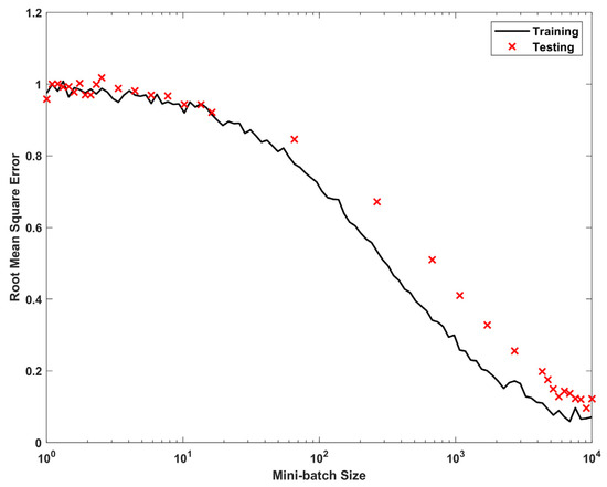
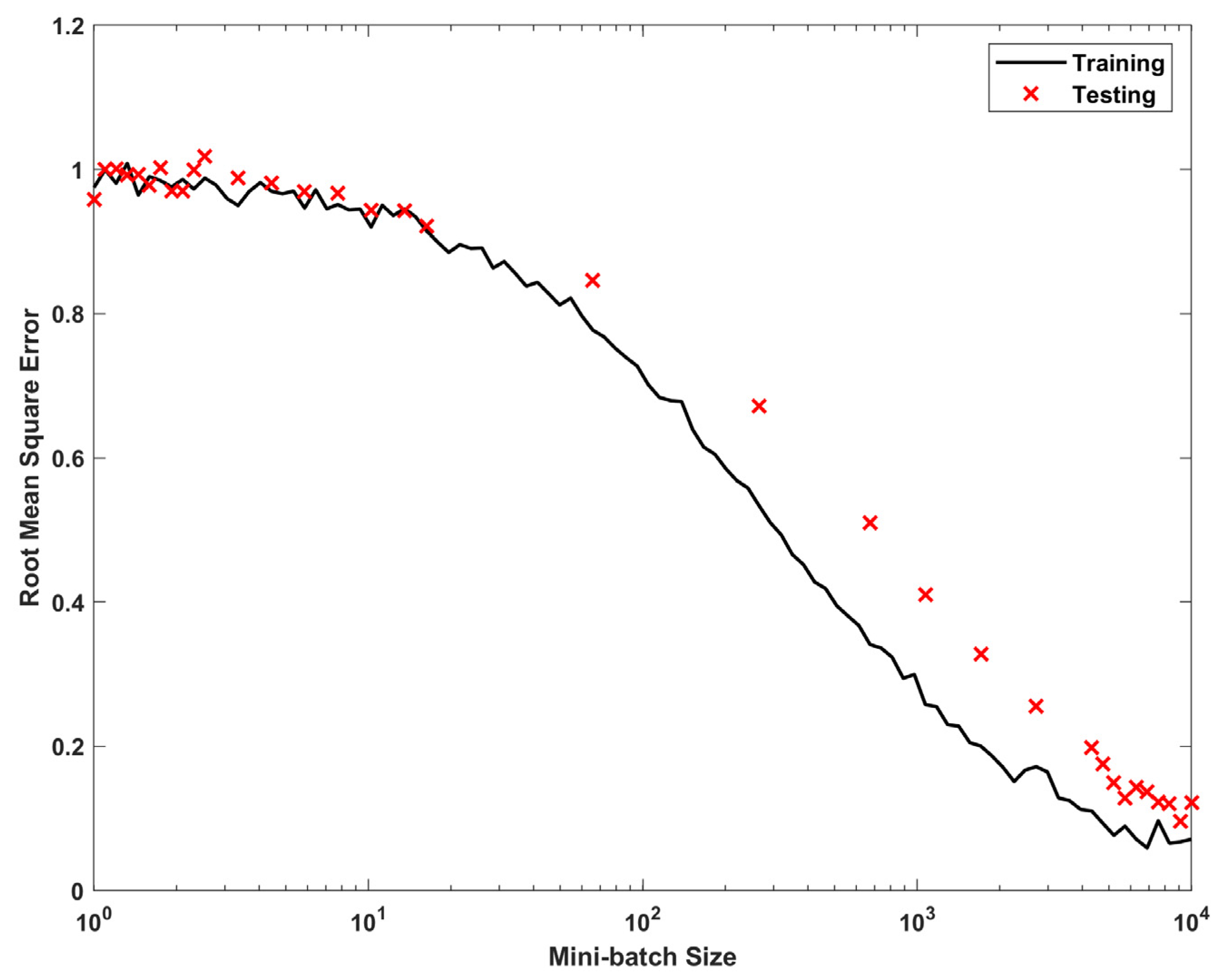
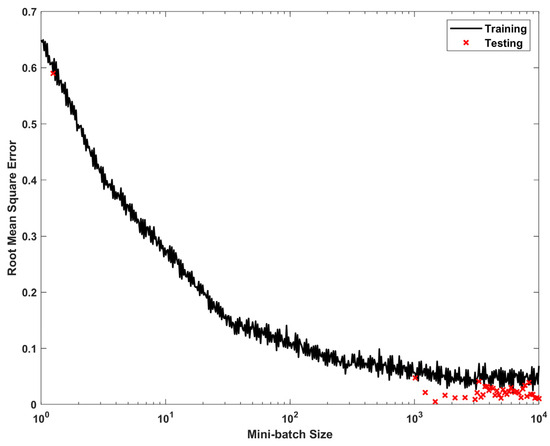
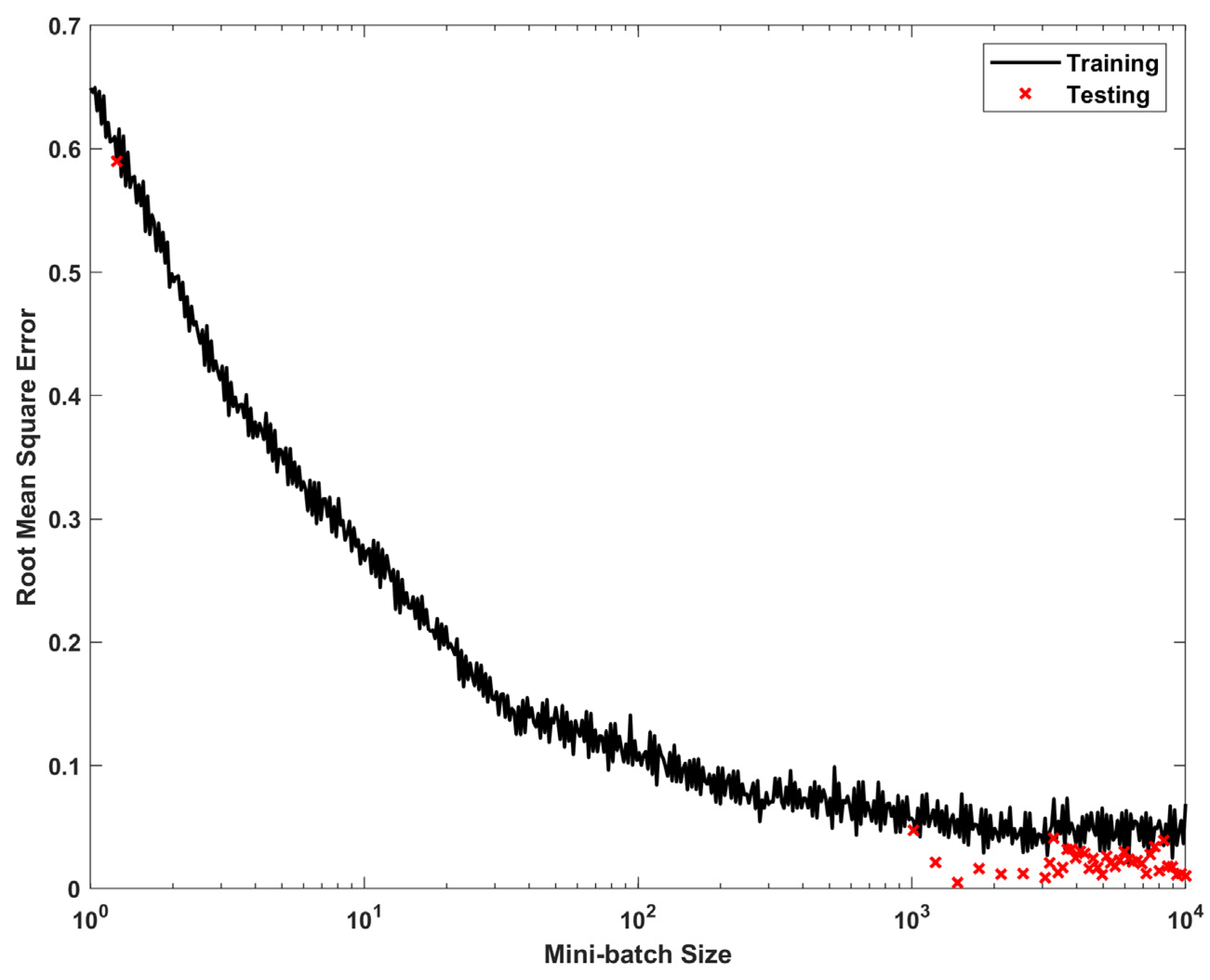
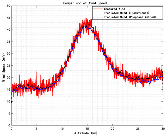
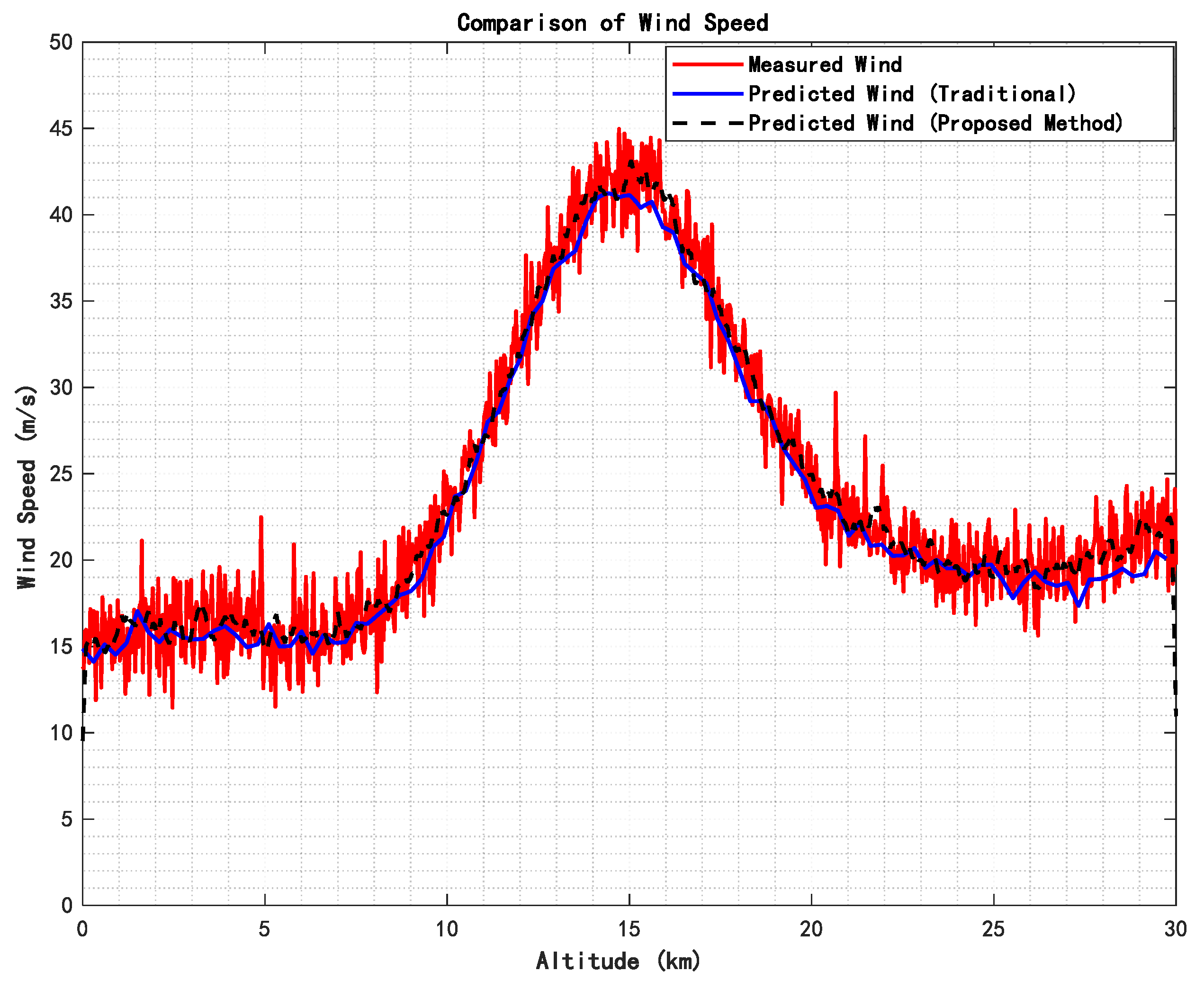
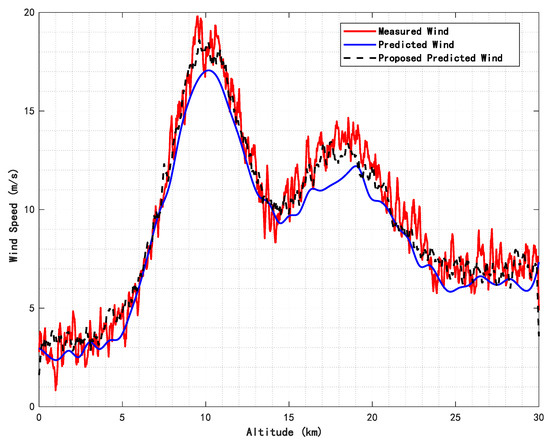
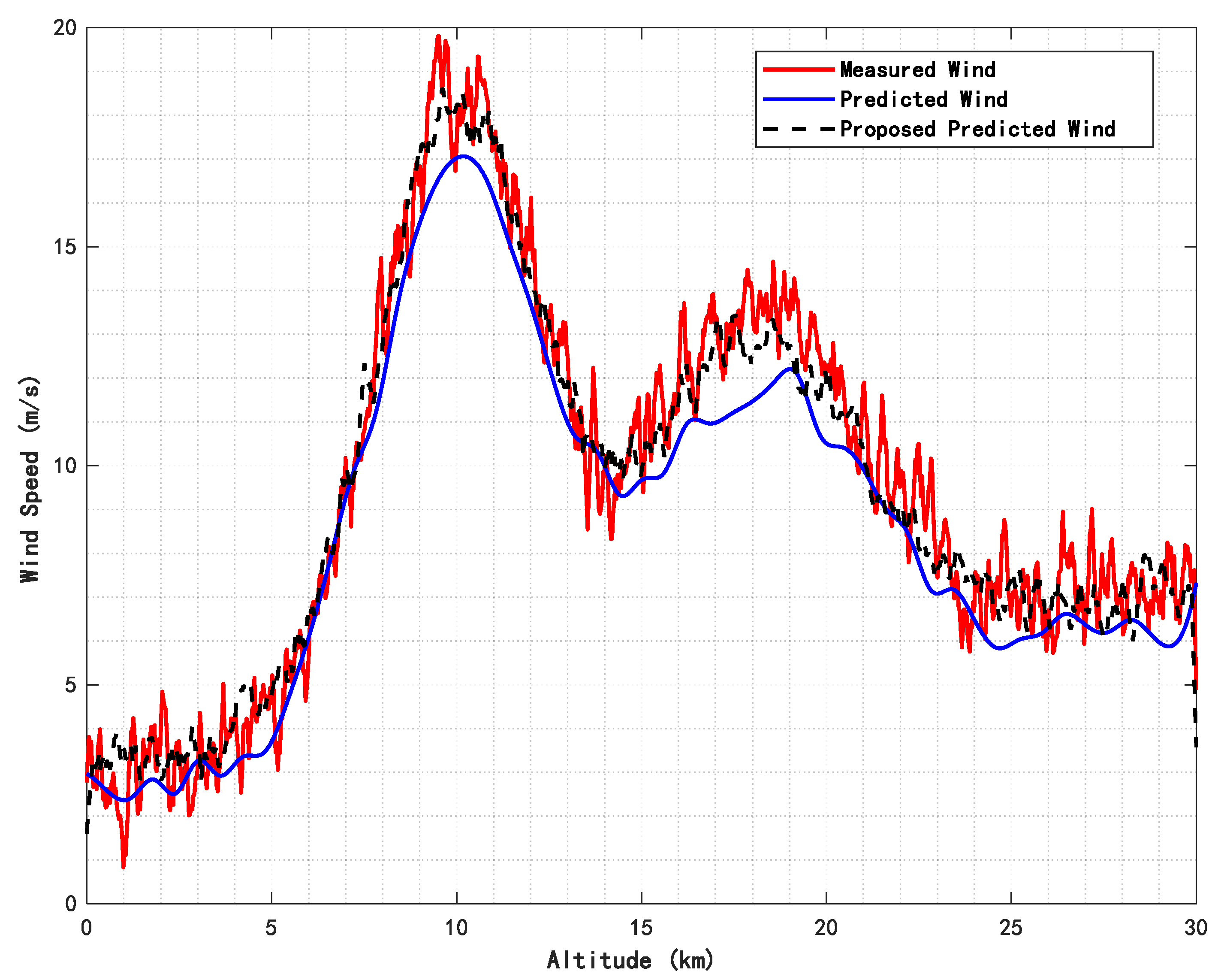
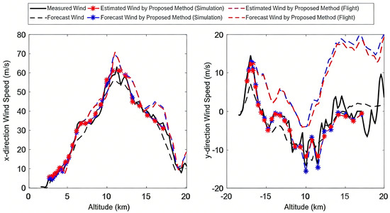
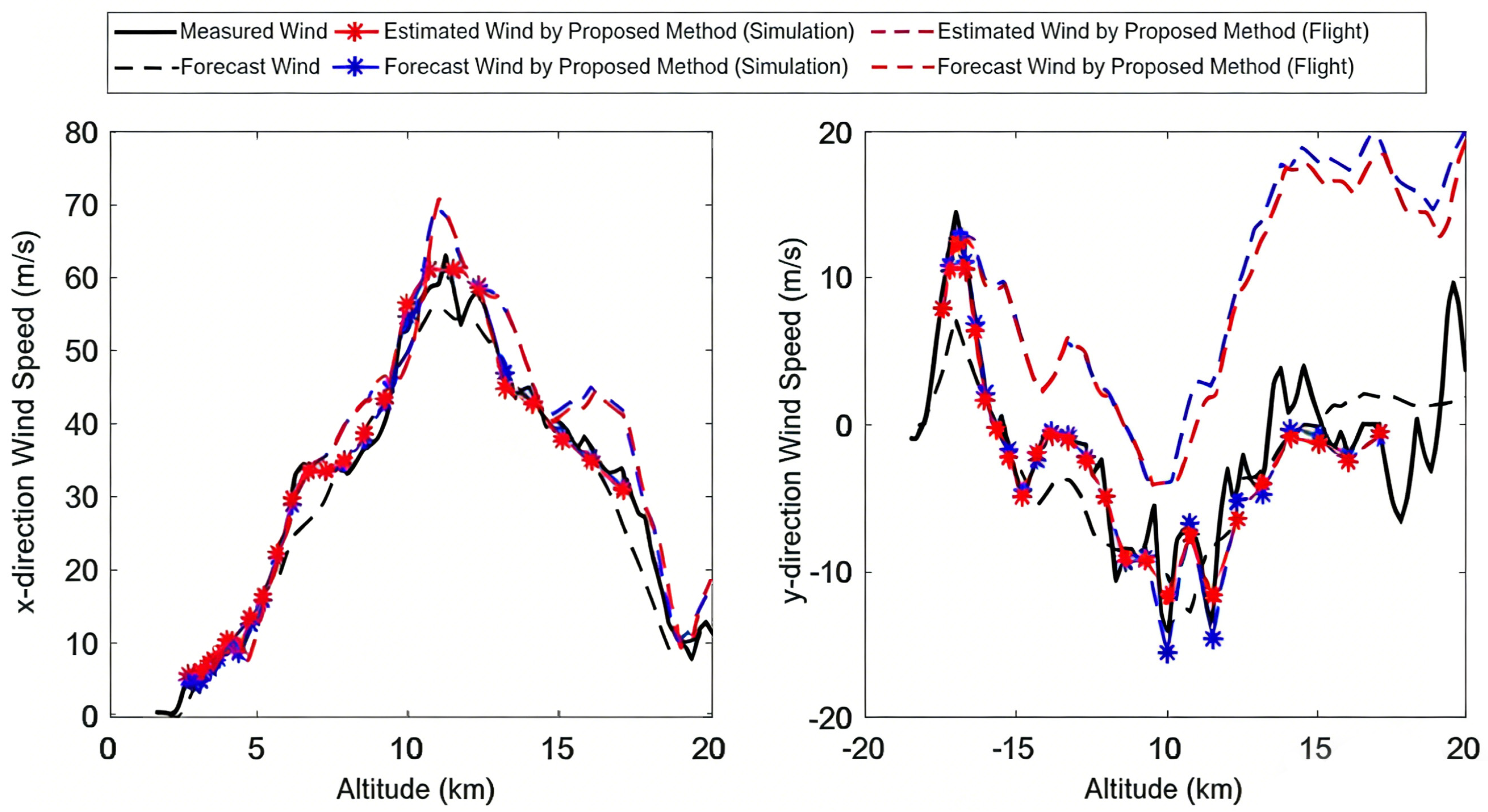
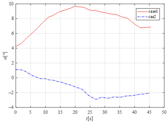
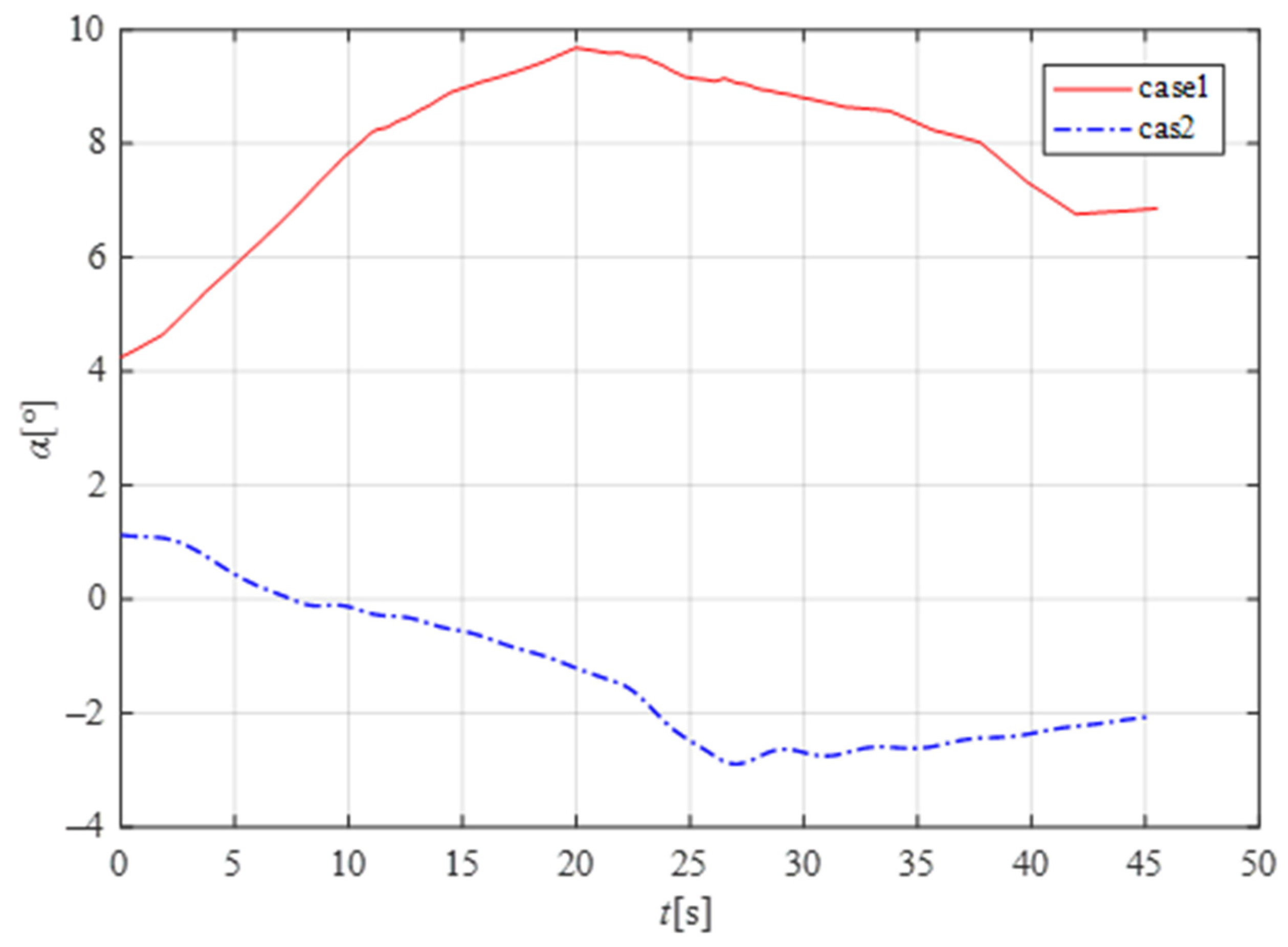
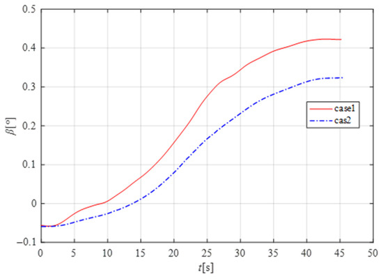
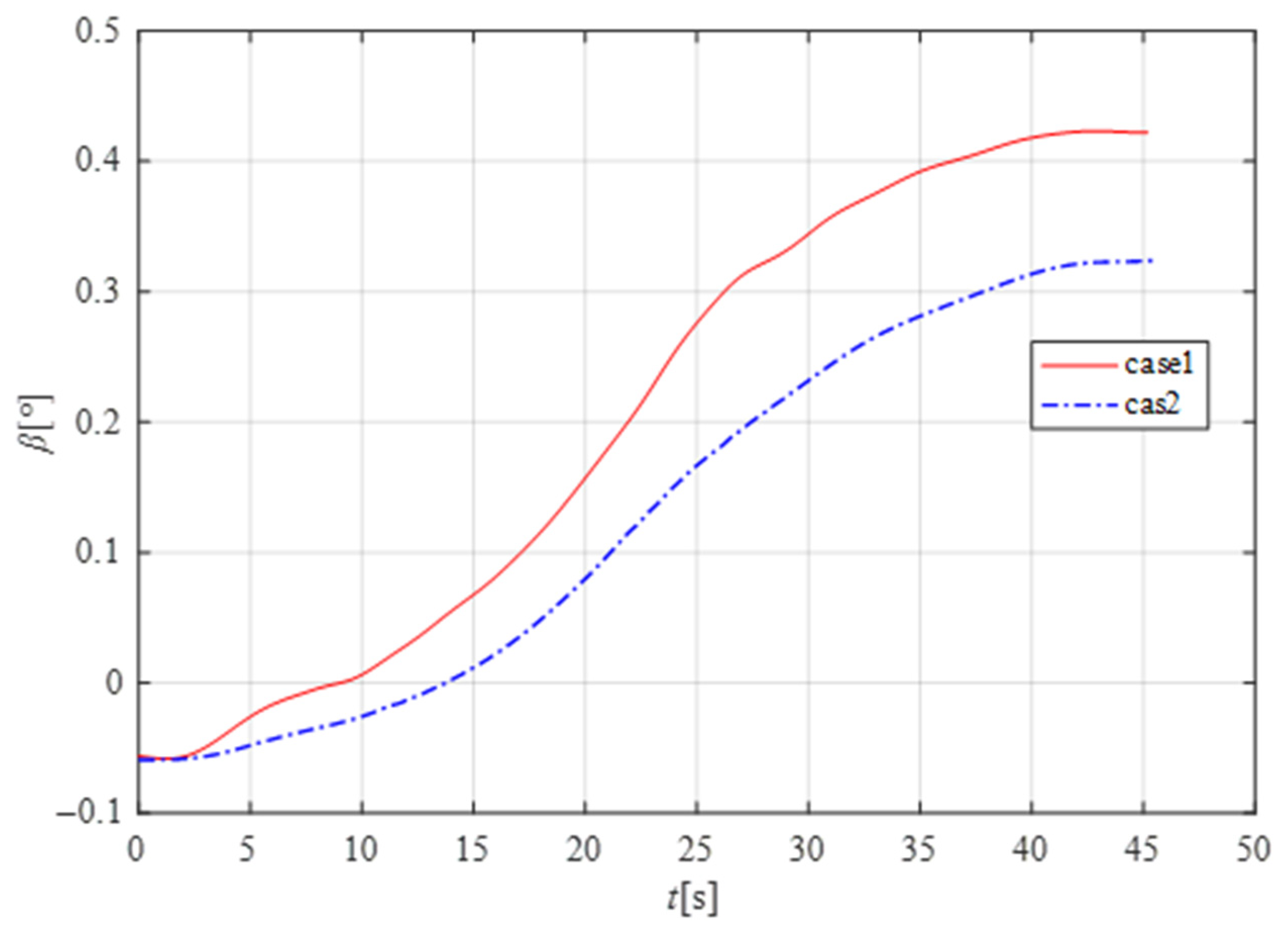
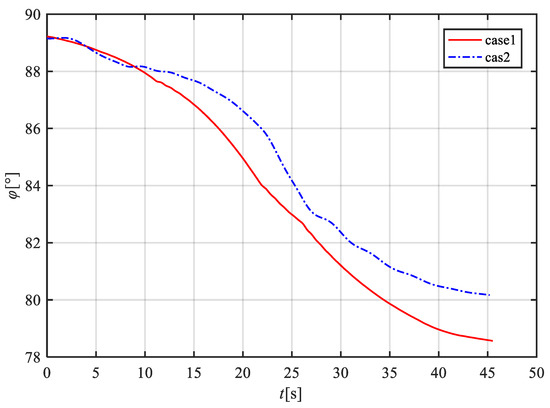
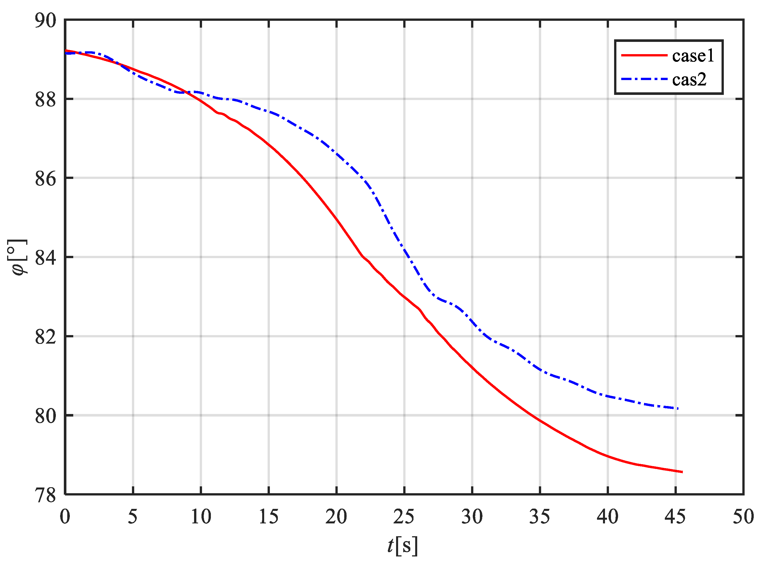
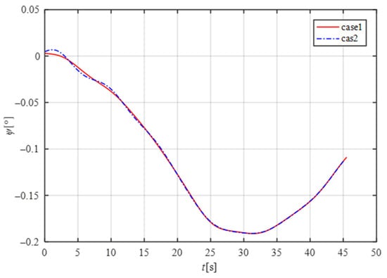
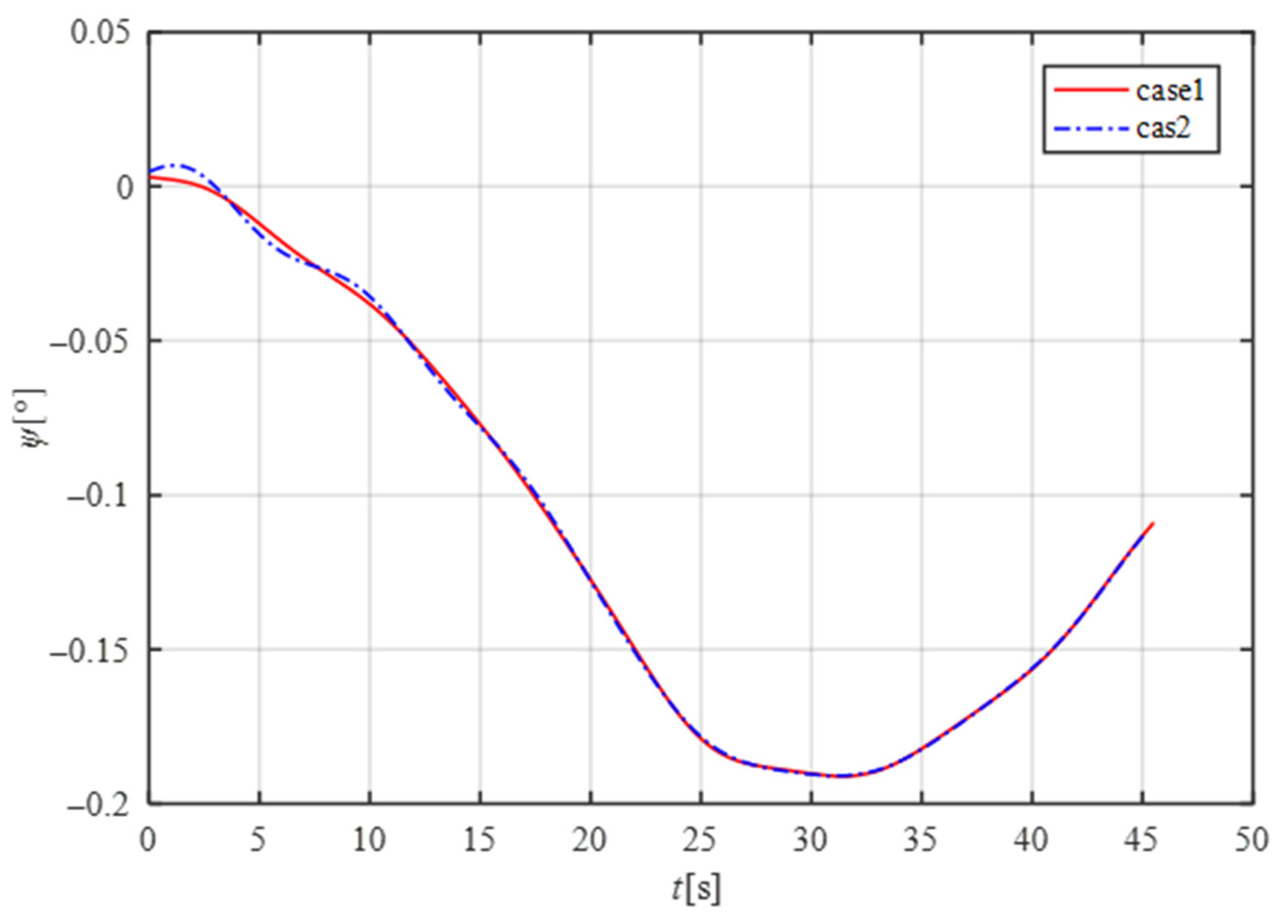
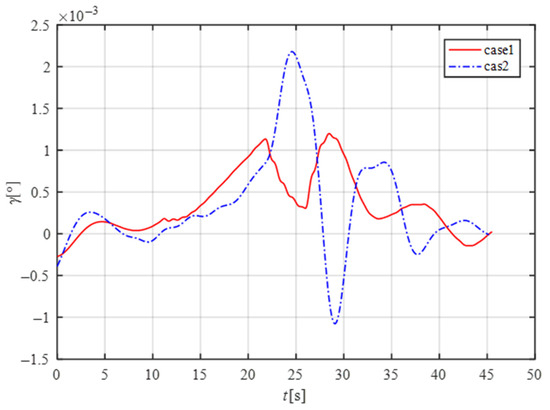
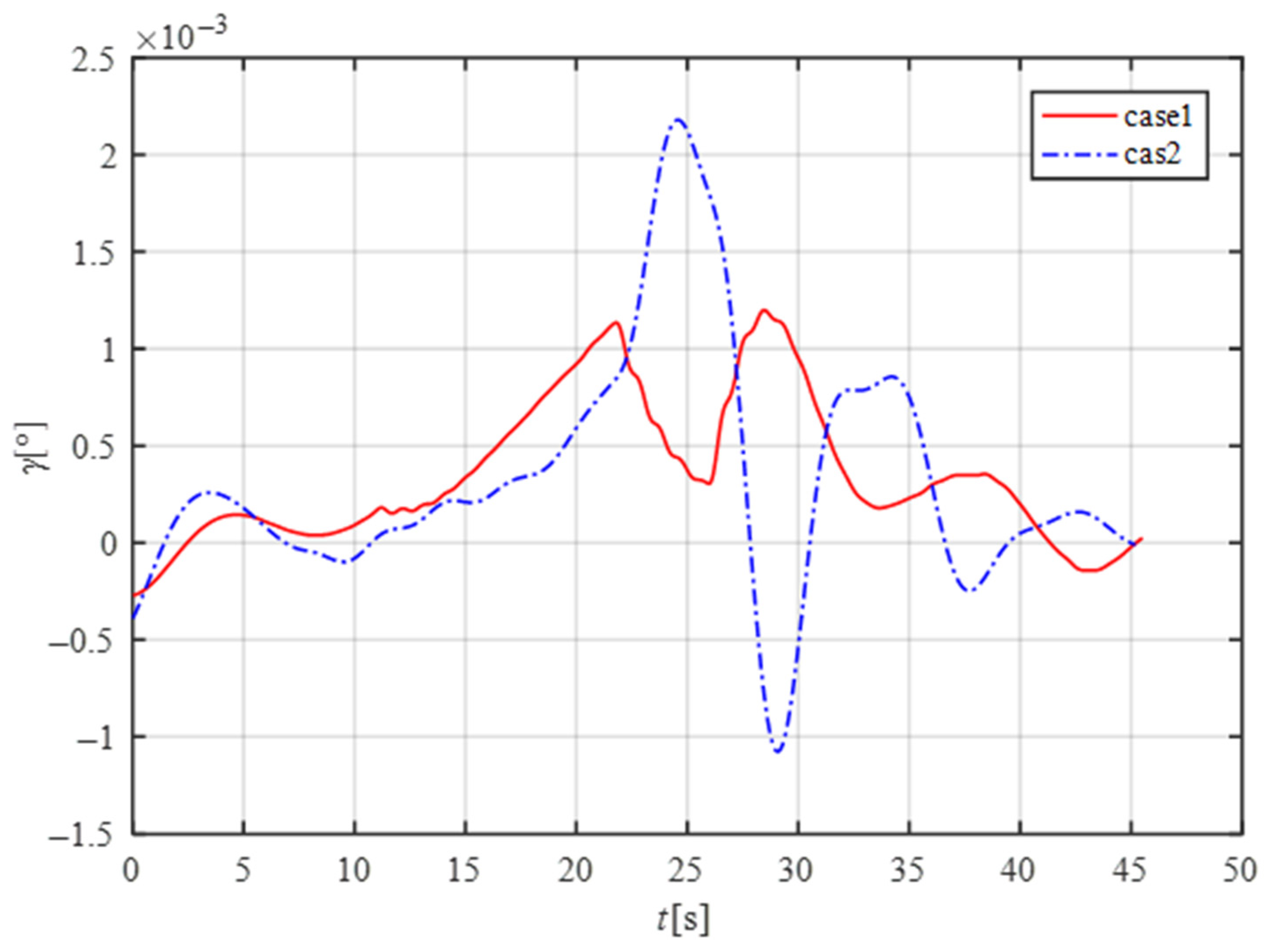
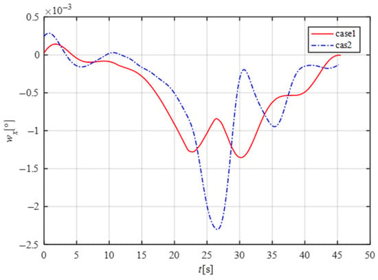
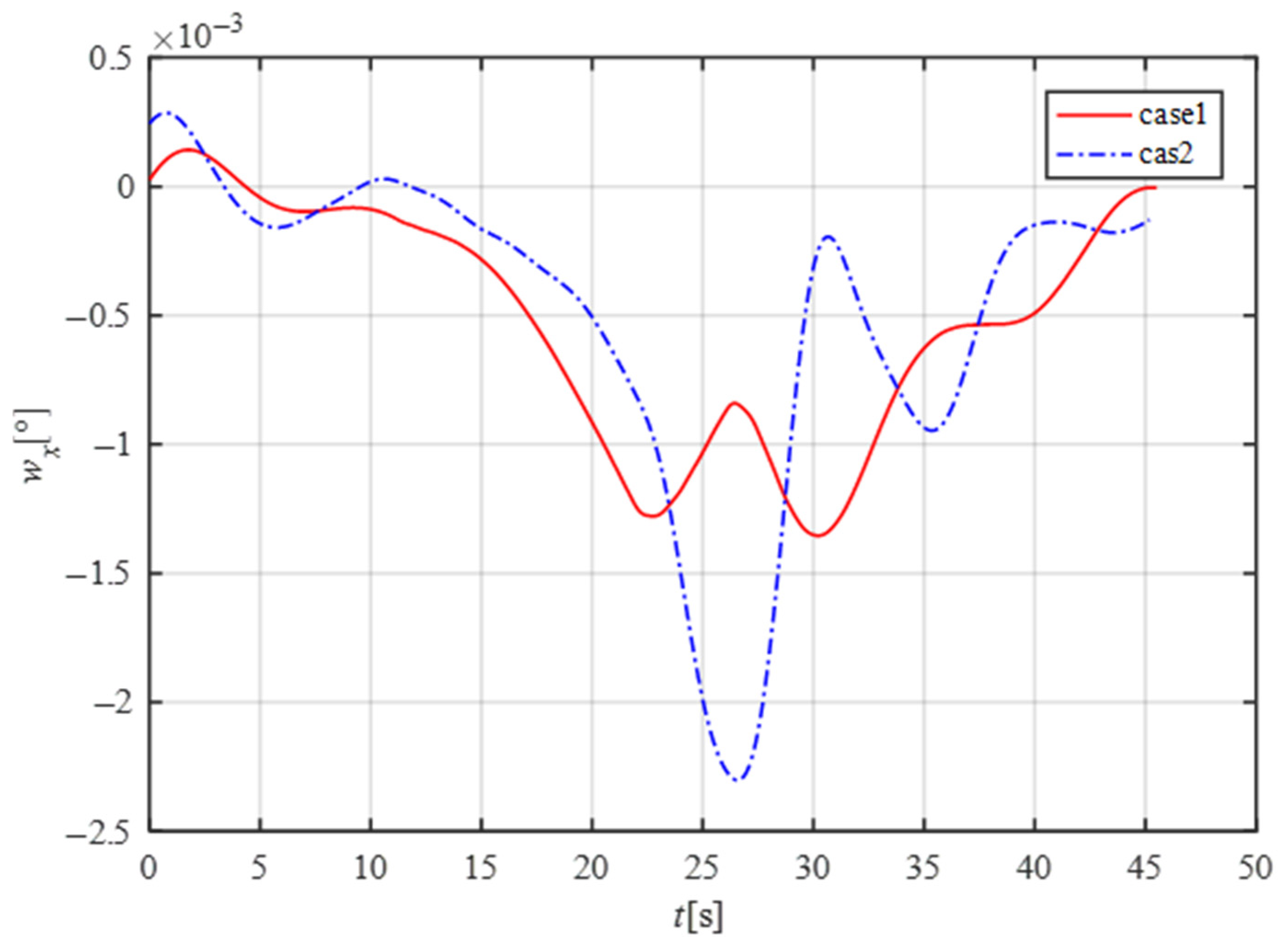
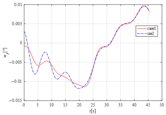
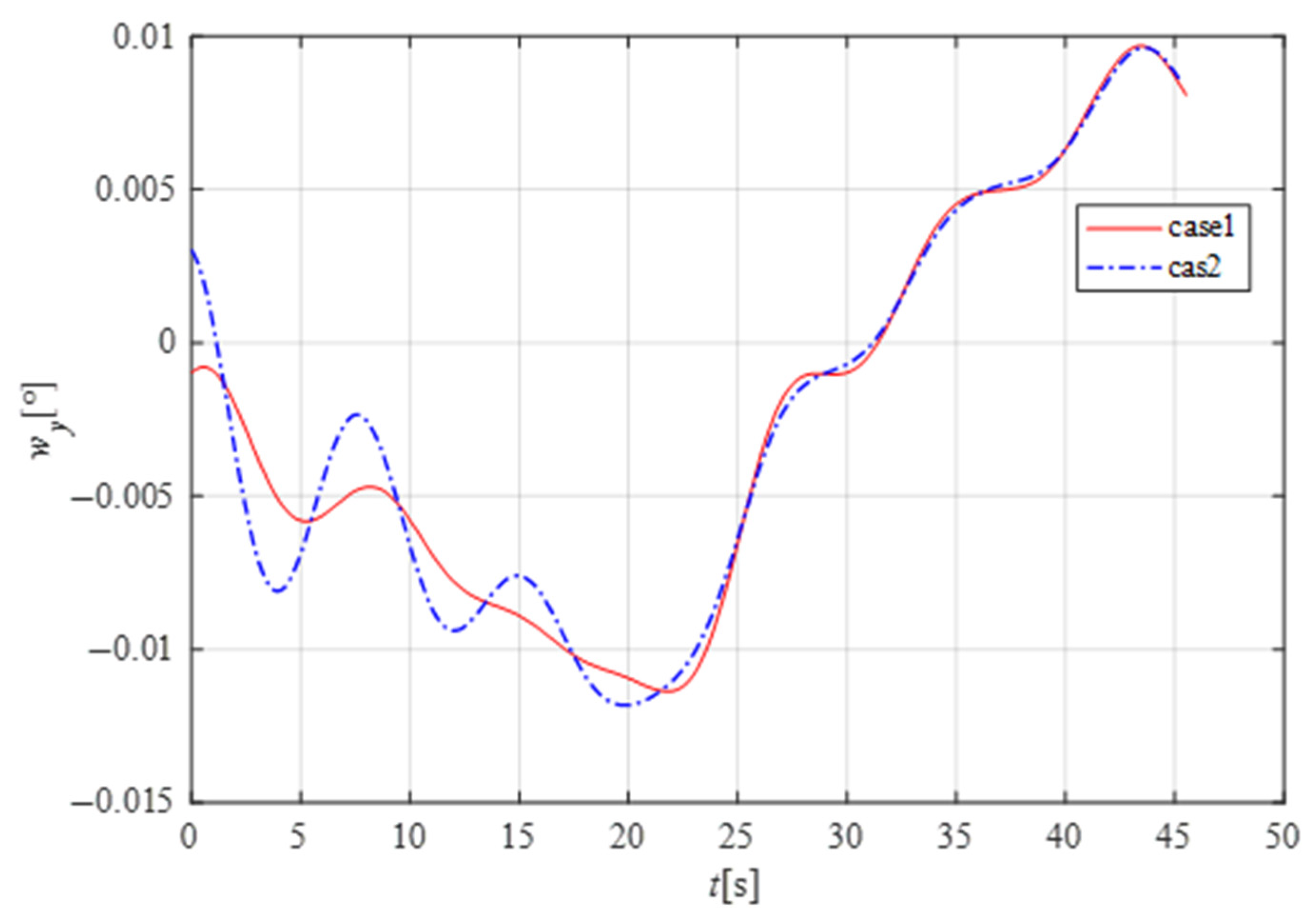
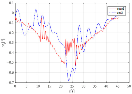
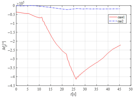
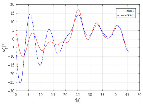
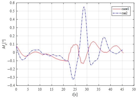

Disclaimer/Publisher’s Note: The statements, opinions and data contained in all publications are solely those of the individual author(s) and contributor(s) and not of MDPI and/or the editor(s). MDPI and/or the editor(s) disclaim responsibility for any injury to people or property resulting from any ideas, methods, instructions or products referred to in the content. |
© 2026 by the authors. Licensee MDPI, Basel, Switzerland. This article is an open access article distributed under the terms and conditions of the Creative Commons Attribution (CC BY) license.