An Infrared Star Identification Algorithm Based on Ordered Angular Distance Verification

Abstract

Short-wave infrared star sensors have become a key technology for all-time attitude determination within the atmosphere, in which the star identification algorithm plays a fundamental role. However, due to the limited number of detectable stars in infrared images, achieving robust and accurate identification remains challenging. To address this issue, this paper proposes a star identification algorithm based on ordered angular distance verification. The algorithm first extracts radial and adjacency features via full-field-of-view sorting to mitigate the impact of “edge loss”. It then employs a fast initial matching that combines hash table lookup with binary search, substantially reducing the number of candidate navigation stars requiring detailed matching. Subsequently, a local search matching procedure corrects index misalignment caused by false or missing stars, while angular distance invariance verification prevents false matches; the combination of these mechanisms significantly enhances the algorithm’s robustness. In simulations using 5000 star images, the proposed algorithm achieves an identification rate of 99.48%. It maintains a rate above 96% under position noise, magnitude noise, and false stars. The average processing time per star image is 10.57 ms, approximately 39% of that required by the conventional grid algorithm (27.01 ms). The simulation results demonstrate that the proposed algorithm achieves high identification accuracy and maintains strong robustness in complex noise environments.

1. Introduction

Star sensors, with their high precision for attitude determination, have been extensively deployed in various space navigation missions [1,2,3]. With continuous advancements in star sensor technology, their application domains are progressively expanding from space to environments within the atmosphere, such as aerial platforms and sea-level scenarios [4]. When operating in these atmospheric conditions, however, traditional visible-light star sensors suffer from significant limitations: their performance is highly susceptible to atmospheric environments, restricting their use to clear nights with an unobstructed field of view (FOV) and minimal ambient light [5,6]. In recent years, research on short-wave infrared (SWIR) focal plane detectors has opened up new possibilities for overcoming these atmospheric limitations [7]. Compared to visible light, SWIR radiation offers advantages including lower atmospheric scattering and higher penetration capability [8,9], which contributes to its greater adaptability to complex weather conditions. Moreover, the daytime sky background radiation intensity in this band is considerably lower than in the visible spectrum. Consequently, the application of SWIR detectors (0.9–1.7 μm) to star sensors has become a significant research focus in the field [10,11], for day-night star stellar navigation.

Star identification is a critical step in all-time navigation for SWIR star sensors, as its identification performance directly determines the correctness of the attitude solution and the real-time capability of the system. Owing to limitations in the inherent material properties and manufacturing processes of SWIR detectors, the resulting star images are often degraded by noise [12]. While image processing techniques can enhance the overall quality of these star images, they cannot fully correct star point distortion, which in turn compromises the centroid extraction accuracy. Furthermore, to suppress intense daytime sky background radiation, all-time star sensors typically employ long focal length designs, which reduce the FOV, diminishing the number of captured stars and increasing the difficulty of identification [13]. Additionally, to ensure sufficient navigation stars within the FOV, the navigation star catalog must be expanded accordingly [14]. This expansion places more stringent performance demands on the star identification algorithm.

Currently, most star identification algorithms are primarily designed for visible-light star images acquired by satellite platforms. The most widely employed star identification algorithm in engineering practice is the triangle algorithm proposed by Liebe [15]. Despite its simplicity, this method relies on low-dimensional feature vectors. As the number of navigation stars grows, the recognition process becomes susceptible to redundant matching and misidentification. To address this issue, Mortari et al. [16] proposed the pyramid algorithm, which builds upon the triangle algorithm by introducing a fourth star to construct higher-dimensional feature descriptors. This approach effectively reduces matching redundancy and improves identification accuracy. However, although the pyramid algorithm exhibits certain robustness against false stars, its time overhead increases significantly as the number of false stars grows. Moreover, when the navigation star database is large, it still cannot completely avoid redundant matching.

Padgett et al. [17] introduced a grid-based algorithm, which encodes star patterns by overlaying a grid for feature matching. While computationally efficient, this method is highly dependent on the correct selection of the nearest neighbor star. To overcome the matching failures of the grid algorithm, Xu et al. [18] proposed an improved algorithm that incorporates the angular distance feature. This enhancement significantly boosts the identification rate and robustness of the original grid algorithm, while the introduced computational complexity inevitably increases the identification time. Zhang et al. [19] proposed a matching method that utilizes both radial and cyclic features of observed stars. In their approach, radial features are employed solely for initial matching to screen candidate stars, while subsequent matching relies exclusively on cyclic features. However, this method suffers from the same dependence on correct initial edge selection as the grid algorithm. Moreover, its identification accuracy is also prone to a sharp decline under conditions of low star density. Sun et al. [20] proposed an improvement to Zhang’s algorithm by calculating the matching degree between reference stars and navigation stars through cumulative angle and distance verification. Although this algorithm achieves a high identification rate and demonstrates strong robustness against noise interference, it involves a complex identification process that is time-consuming.

As neural network technology continues to advance, deep learning-based star identification algorithms have gradually become a research hotspot. Wang et al. [21] employed a convolutional neural network (CNN) based on Vgg16 with data augmentation to achieve robust star identification against various noises. However, its reliance on multiple orientation attempts incurs computational overhead. To address the degradation of identification accuracy caused by poor star point positioning under dynamic conditions, Han et al. [22] proposed an end-to-end star identification network based on the attention mechanism. Their method encodes the positional information of star points and focuses on extracting relative position features. Although it exhibits strong robustness against position noise, the algorithm suffers from long identification time and high memory consumption due to its complex network structure.

Despite continuous innovations in star identification algorithms, a prominent gap remains in the research on algorithms for infrared star images, which are characterized by narrow FOV and a relatively limited number of identifiable stars [23,24,25]. To address the distinct challenges of infrared star images, this paper proposes an identification algorithm that achieves real-time performance while remaining robust against false stars, position noise, and magnitude noise. The algorithm begins by sorting neighboring stars in ascending order of their angular distance from the reference star and selects the k-nearest to form a sequence. Rotation-invariant features are then constructed by calculating both the angular distances from each star to the reference star and the angular distances between consecutive stars within the sequence. Using these features, fast initial matching is first performed via a hash table to efficiently filter candidate navigation stars. A local search matching algorithm is then employed to compute the matching scores between the reference star and each candidate, with the candidate achieving the highest score selected as the final identification result. Once the reference star is successfully identified, the stars in its neighboring star sequence are also identified. This process increases the number of reliably identified stars and provides a foundation for higher-precision attitude determination.

2. Algorithm Description

In this section, the implementation details of the star identification algorithm based on ordered-feature matching are elaborated. It first outlines the feature extraction principles for navigation stars, then describes the construction and structure of the navigation database. Finally, it presents the process of star identification, including feature extraction from star images, feature matching, and the overall identification process.

2.1. Feature Extraction and Navigation Database Construction

2.1.1. Feature Extraction for Navigation Star

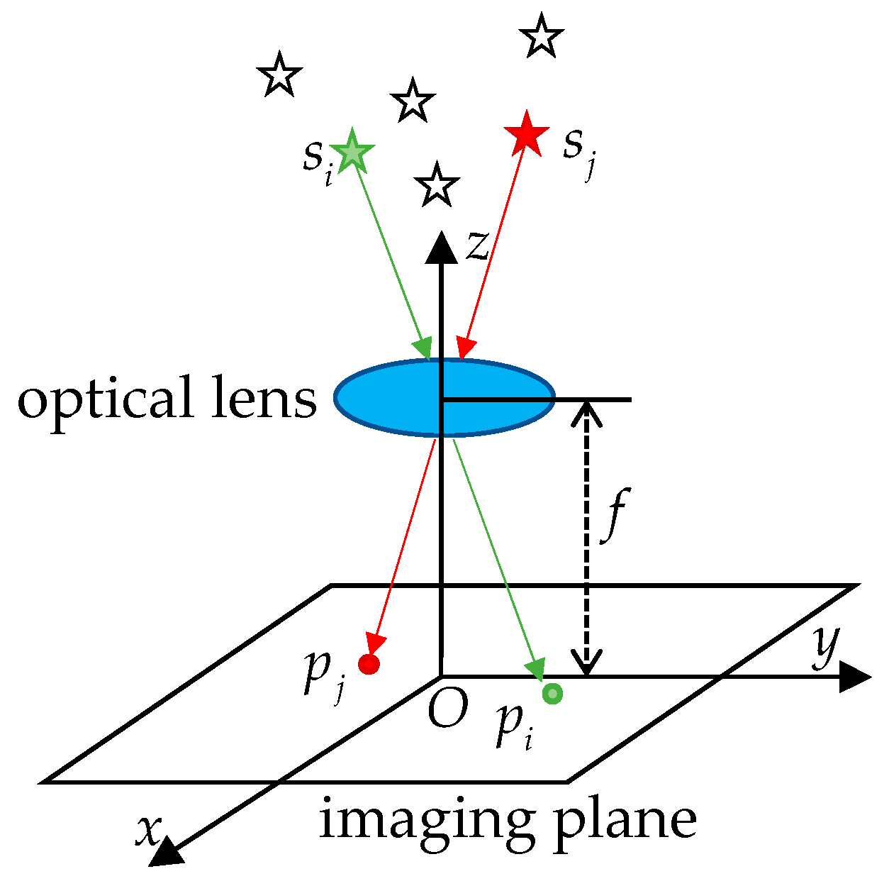
Compared to visible-light star images, infrared star images typically contain fewer stars and pose greater identification challenges. Therefore, efficient feature extraction from navigation stars is a crucial prerequisite for utilizing the information in infrared star image and enhancing star identification accuracy. The feature extraction algorithm proposed in this paper is based on the imaging model of the star sensor. As shown in Figure 1, the coordinate system $O-xyz$ represents the star sensor coordinate system, which coincides with the imaging coordinate system.

Let $s_i$ and $s_j$ denote two stars on the celestial sphere, with ${\alpha }_i$ and ${\alpha }_j$ being their right ascension, ${\delta }_i$ and ${\delta }_j$ being their declination. Their direction vectors in the celestial coordinate system, $v_i$ and $v_j$, are expressed as

$$v_i=\left[\begin{array}{c}\cos {\alpha }_i\cos {\delta }_i\\ \sin {\alpha }_i\cos {\delta }_i\\ \sin {\delta }_i\end{array}\right] ,v_j=\left[\begin{array}{c}\cos {\alpha }_j\cos {\delta }_j\\ \sin {\alpha }_j\cos {\delta }_j\\ \sin {\delta }_j\end{array}\right].$$

(1)

Assuming $p_i$ and $p_j$ are the image points corresponding to stars $s_i$ and $s_j$, with $(x_i,y_i)$ and $(x_j,y_j)$ being their ideal centroid coordinates, and $f$ being the focal length of the star sensor, the unit vector expressions for $s_i$ and $s_j$ in the star sensor coordinate system are

$$w_i={\displaystyle \frac{1}{\sqrt{x_i^2+y_i^2+f^2}}}\left[\begin{array}{c}-x_i\\ -y_i\\ f\end{array}\right],w_j={\displaystyle \frac{1}{\sqrt{x_j^2+y_j^2+f^2}}}\left[\begin{array}{c}-x_j\\ -y_j\\ f\end{array}\right].$$

(2)

The angular distance between the stars $s_i$ and $s_j$ in the celestial coordinate system is

$$d_{ij}=\arccos (v_i·v_j).$$

(3)

The angular distance between the imaging points $p_i$ and $p_j$ in the star sensor coordinate system is

$$d_{ij}^{\prime }=\arccos (w_i·w_j).$$

(4)

According to imaging principles, under ideal conditions, $d_{ij}^{\prime }$ should equal $d_{ij}$. Owing to the invariance of angular distance during the imaging process, it serves as an ideal feature for constructing star pattern models.

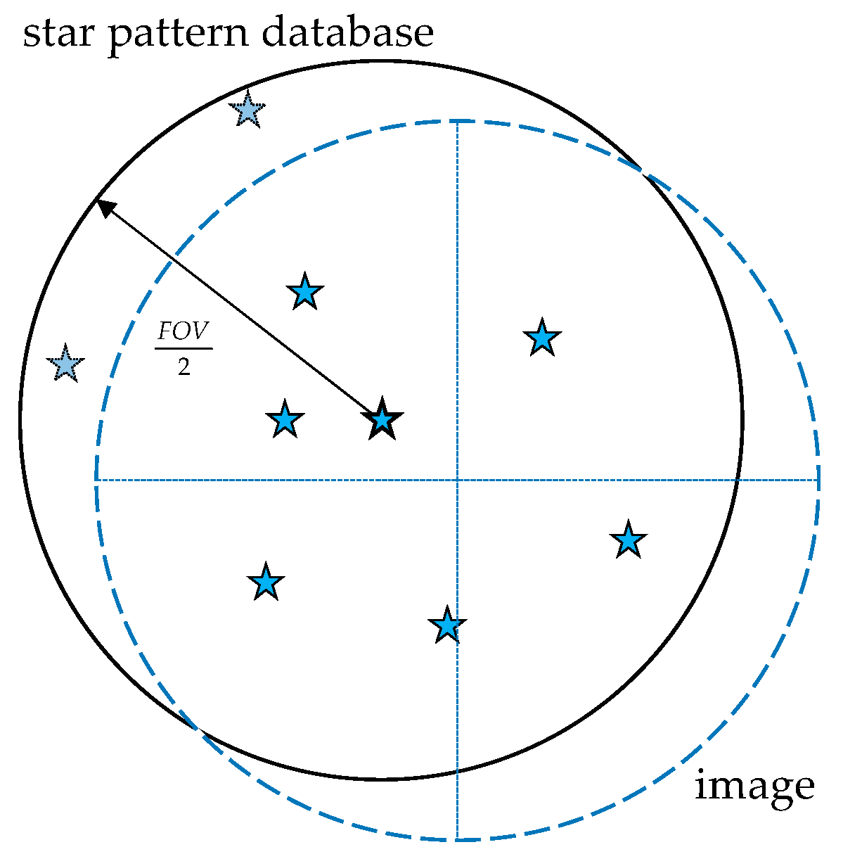
However, a practical challenge arises when constructing star patterns based on this invariant angular distance. As shown in Figure 2, when the observed primary star is not located at the origin, neighboring stars at greater distances may fall outside the observation FOV. This leads to a situation where the observation vector lacks some elements compared to the pattern vector, a phenomenon referred to as “edge loss” [26]. To mitigate the distortion of features caused by edge loss, existing pattern-based identification algorithms typically construct feature vectors for navigation stars within a fixed radius smaller than the FOV [27,28]. However, in conditions of a narrow FOV and a finite number of stars, this method severely limits the number of usable stars, resulting in inadequate feature dimensions, which in turn leads to lower identification accuracy. To address this limitation, a feature construction method using full-FOV sorting is presented.

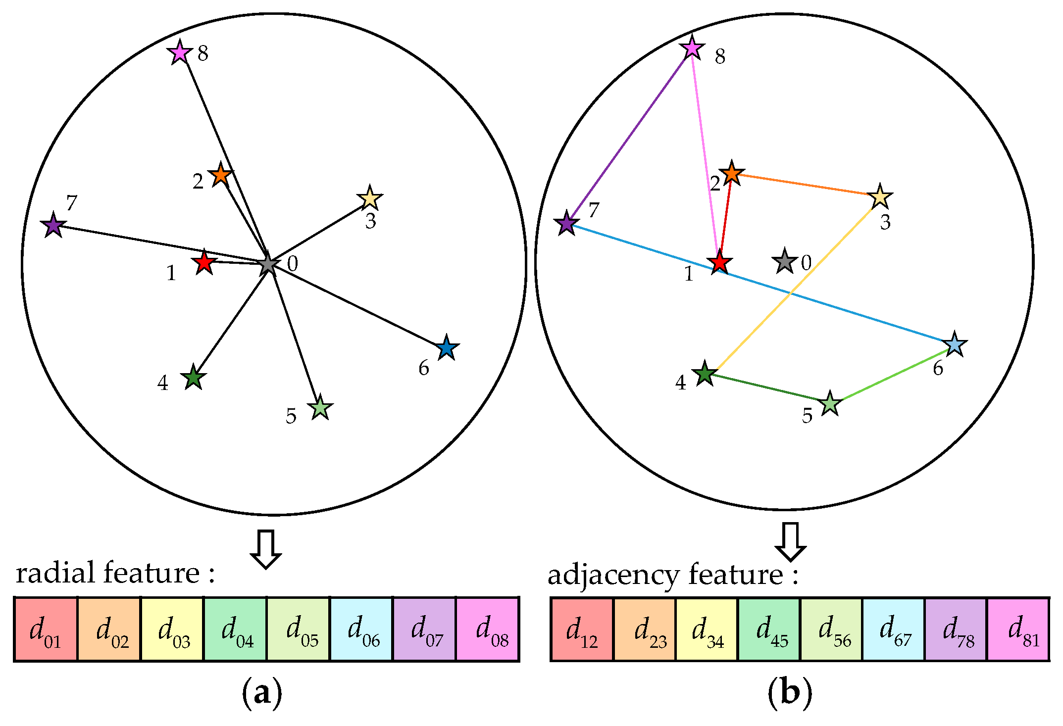
Based on the imaging model of the star sensor, the proposed algorithm constructs pattern feature for a navigation star using celestial coordinates. As shown in Figure 3, with the navigation star $S_0$ as the center, up to $k$ nearest stars within its FOV are selected as neighboring stars. These are then sorted in ascending order of their angular distance from $S_0$, forming the neighboring star sequence $S=\{S_1,S_2,\dots ,S_n\}$ where $n\le k$ corresponds to the actual number of available stars. Each adjacent pair in the sequence (including the last and the first) is defined as feature neighbors. The radial feature vector $V_{\mathrm{Nr}}=[d_{01},d_{02},\dots ,d_{0n}]$ is formed by sequentially calculating the angular distance between each star in $S$ and the navigation star $S_0$. Simultaneously, the adjacency feature vector $V_{\mathrm{Na}}=\left[d_{12},d_{23},\dots ,d_{n1}\right]$ is constructed by sequentially calculating the angular distance between each star and its subsequent star in $S$, including the angular distance between the last star and the first one. Here, $d_{ij}$ denotes the angular distance between $S_i$ and $S_j$, calculated using Equation (3).

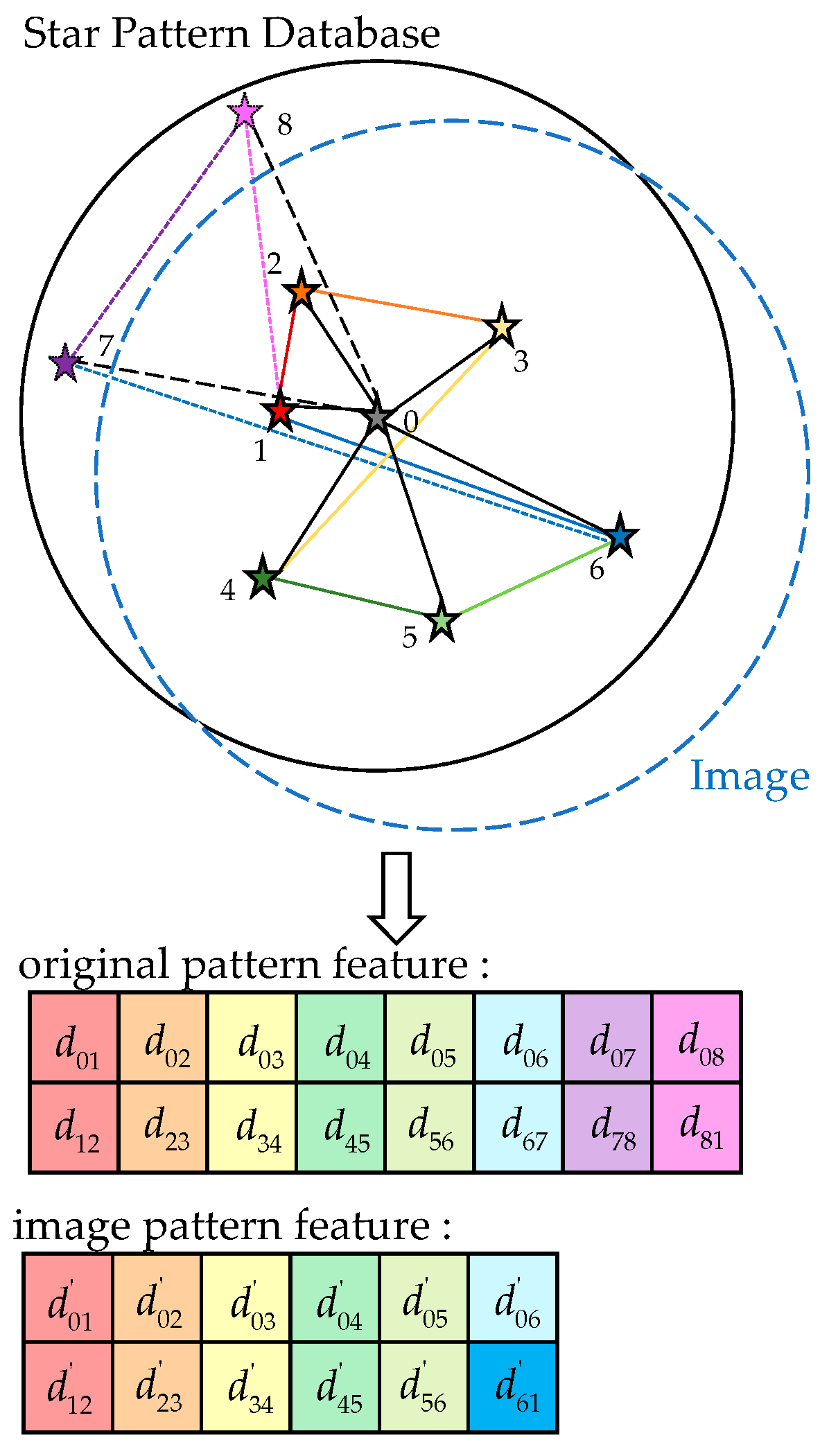
This method demonstrates considerable robustness to the loss of edge stars, as it fully utilizes the remaining star information while preserving the features of the closest stars. As shown in Figure 4, when edge stars (Star 7, Star 8) are lost, although the corresponding positional pattern features are affected, the navigation star’s feature information is retained to the greatest extent possible.

2.1.2. Construction of the Navigation Database

This section illustrates the construction of a navigation database using a star sensor with a FOV of ${4.312}^{°}\times {4.312}^{°}$, a limiting magnitude of 4 Mv, and a detection range in the short-wave infrared band (1.0 μm–1.7 μm). The Two Micron All-Sky Survey (2MASS) All-Sky Point Source Catalog serves as the fundamental catalog. By incorporating filter parameters, the H-band magnitude data is directly utilized as the instrumental magnitude. After excluding variable stars and unresolved binary stars, stars with magnitudes ≤ 4 Mv are selected based on the sensitivity threshold of the star sensor, yielding a final navigation star catalog of 10,441 stars. Taking each navigation star as center, stars within the star sensor’s FOV are identified as its neighbors. The radial and adjacency features of these navigation stars are then extracted using the method described in Section 2.1.1, and assembled into a pattern feature database. As shown in

Table 1. Basic structure of the navigation database.

Navigation Star Table	Pattern Database
Star Index	Radial Feature
Right Ascension	Adjacency Feature
Declination	Neighbor Star Indices

, the basic structure of the navigation database primarily comprises two parts: a navigation star catalog, comprising star indices, right ascension, and declination data; and a pattern feature database, containing radial features, adjacency features, and neighbor star indices for each navigation star.

Meanwhile, to enhance identification efficiency, a hash table based on radial feature quantization is constructed for initial matching. First, the radial feature elements $d_{\mathrm{r}i}$ of each navigation star are quantized by mapping the angular distance values into integer keys

$$q_i=⌊{\displaystyle \frac{d_{\mathrm{r}i}}{{\epsilon }_{\mathrm{d}}}}⌋,$$

(5)

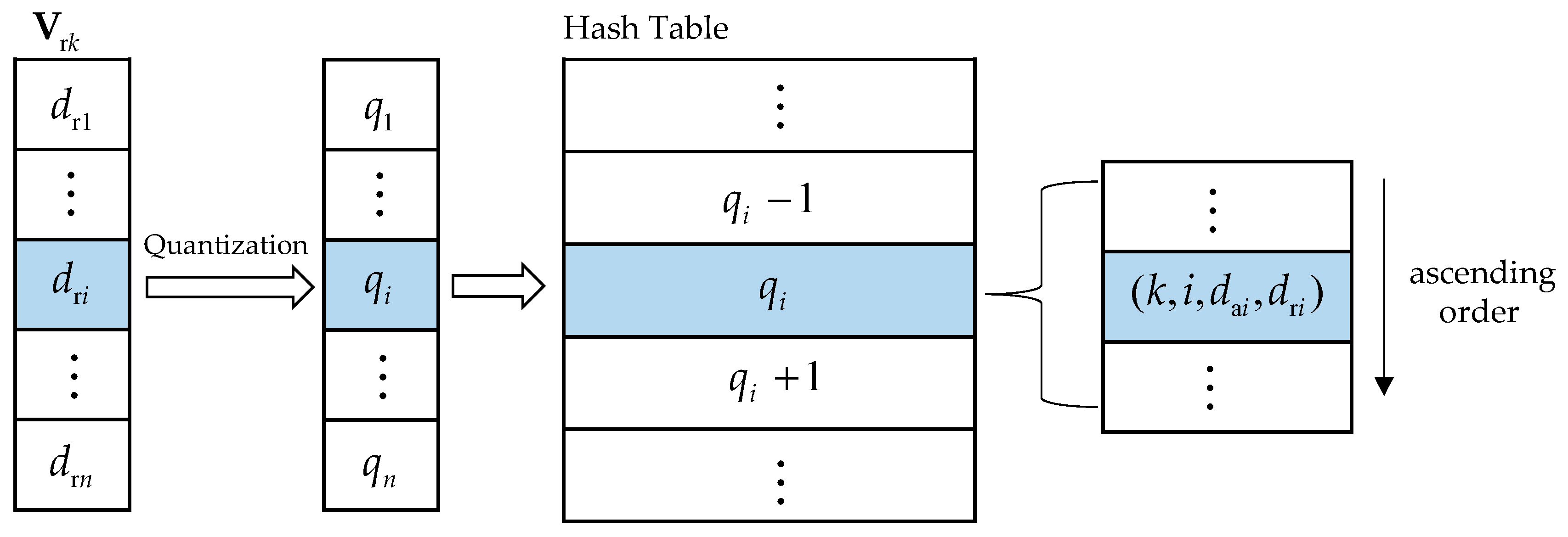
where $⌊\cdot ⌋$ denotes the floor function and ${\epsilon }_{\mathrm{d}}$ is the matching error threshold. Each quantization key corresponds to a storage unit, which stores a list of tuples containing the navigation star index k, the neighbor star sequence number i, the adjacency feature value $d_{\mathrm{a}i}$, and the radial feature value $d_{\mathrm{r}i}$. To enable fast matching of adjacency features, the tuples within each list are sorted in ascending order of adjacency feature values. The detailed construction process of the hash table is illustrated in Figure 5, where ${\mathrm{V}}_{\mathrm{r}k}$ denotes the radial feature vector of the k-th navigation star.

2.2. Star Identification Algorithm Design

2.2.1. Feature Extraction for Star Image

The star identification process begins by selecting the star point closest to the image center as the reference star $S_{\mathrm{R}0}$. Then, the angular distances between $S_{\mathrm{R}0}$ and all other stars within its FOV are calculated using Equation (4). Up to $k$ stars with the smallest angular distances are chosen as neighboring stars; these are then sorted in ascending order to form a sequence $\{S_{\mathrm{R}1},S_{\mathrm{R}2},\dots ,S_{\mathrm{R}m}\}$ where $m\le k$ denotes the actual number of neighboring stars available. A radial feature vector $V_{\mathrm{Rr}}=[d_{01}^{\prime },d_{02}^{\prime },\dots ,d_{0m}^{\prime }]$ is generated from the angular distances between each star in this sequence and the reference star, while an adjacency feature vector $V_{\mathrm{Ra}}=[d_{12}^{\prime },d_{23}^{\prime },\dots ,d_{m1}^{\prime }]$ is formed by calculating the angular distances between all adjacent star pairs in the sequence. Here, $d_{ij}^{\prime }$ denotes the angular distance between $S_{\mathrm{R}i}$ and $S_{\mathrm{R}j}$, calculated using Equation (4). The constructed features have the following properties:

• Uniqueness: A high-dimensional feature characterizing the local spatial structure of the reference star is generated from angular distances of finite stars. Owing to its strong discriminative capacity, this feature significantly reduces redundant matches and lowers the potential for false matches, even when searching through extensive navigation star catalogs.
• Stability: As the feature is composed of angular distances, it is inherently scale-invariant during imaging. Moreover, the feature pattern exhibits considerable robustness against “edge loss”.
• Ordered Sequence: The feature sequence is systematically arranged in ascending order of the angular distance between neighboring stars and the reference star. This ordering ensures that the matching process can proceed through a sequential comparison according to the index order, thereby effectively reducing the computational complexity.

2.2.2. Initial Matching

To improve the efficiency of star matching, initial matching of a reference star against navigation stars is performed using the hash table. For each position u in the reference star’s feature sequence, its radial feature value $d_{\mathrm{r}u}^{\prime }$ and adjacency feature value $d_{\mathrm{a}u}^{\prime }$ are obtained, and the quantized value $q_u^{\prime }$ of the radial feature is calculated using Equation (5). To mitigate the impact of quantization errors, the search range is expanded to three adjacent quantization units $\{q_u^{\prime }-1,q_u^{\prime },q_u^{\prime }+1\}$.

Within each unit, leveraging the ordered arrangement of adjacency features, a binary search is conducted to identify all navigation star entries that satisfy

$$\left|d_{\mathrm{a}v}-d_{\mathrm{a}u}^{\prime }\right|\le {\epsilon }_{\mathrm{d}},$$

(6)

where $d_{\mathrm{a}v}$ is the adjacency feature value corresponding to the v-th position in that navigation star’s feature sequence, as stored in the hash table. Further verification is then performed to check whether its corresponding radial feature $d_{\mathrm{r}v}$ meets

$$\left|d_{\mathrm{r}v}-d_{\mathrm{r}u}^{\prime }\right|\le {\epsilon }_{\mathrm{d}}.$$

(7)

If both conditions are satisfied, the navigation star index is added to the candidate star set. The matched feature positions (u,v) between the current reference star and the navigation star are recorded, with no duplicate entries recorded for the same navigation star.

This stage, through hash table lookup based on quantized features, reduces the number of navigation stars requiring further detailed matching by approximately two orders of magnitude, laying the foundation for enhancing the overall efficiency of the algorithm.

2.2.3. Detailed Matching

Local Search Matching for Feature Sequences

To address the index misalignment between feature sequences caused by false or missing stars, the algorithm employs a local search strategy based on the ordering of radial features, aiming to establish correct correspondences between the reference star and candidate star feature sequences.

Let the radial and adjacency feature vectors of the reference star be $V_{\mathrm{Rr}}=[d_{\mathrm{r}1}^{\prime },d_{\mathrm{r}2}^{\prime },\dots ,d_{\mathrm{r}m}^{\prime }]$ and $V_{\mathrm{Ra}}=[d_{\mathrm{a}1}^{\prime },d_{\mathrm{a}2}^{\prime },\dots ,d_{\mathrm{a}m}^{\prime }]$, respectively, those of a candidate star currently being matched be $V_{\mathrm{Cr}}=[d_{\mathrm{r}1},d_{\mathrm{r}2},\dots ,d_{\mathrm{r}n}]$ and $V_{\mathrm{Ca}}=[d_{\mathrm{a}1},d_{\mathrm{a}2},\dots ,d_{\mathrm{a}n}]$, with m and n denoting their respective feature dimensions. The matching then starts from the beginning of the sequences.

Let the current matching positions in the reference and candidate star feature sequences be i and j, respectively. Since the matching of adjacency features depends on successful radial feature matching at the corresponding positions, the algorithm begins at the candidate star index j and proceeds forward along its radial feature sequence to identify all indices t that satisfy the constraint

$$\left|d_{\mathrm{r}t}-d_{\mathrm{r}i}^{\prime }\right|\le {\epsilon }_{\mathrm{d}}.$$

(8)

Due to the ordering of the radial features, the search terminates upon first encountering $d_{\mathrm{r}t}-d_{\mathrm{r}i}^{\prime }>{\epsilon }_{\mathrm{d}}$. All such indices t constitute the set $T_{\mathrm{r}i}$.

Subsequently, for each candidate index t in the set $T_{\mathrm{r}i}$, the algorithm verifies its adjacency feature to determine if it satisfies the threshold condition

$$\left|d_{\mathrm{a}t}-d_{\mathrm{a}i}^{\prime }\right|\le {\epsilon }_d.$$

(9)

All such indices t constitute the set $T_{\mathrm{a}i}$. Based on the index set results, the algorithm proceeds as follows:

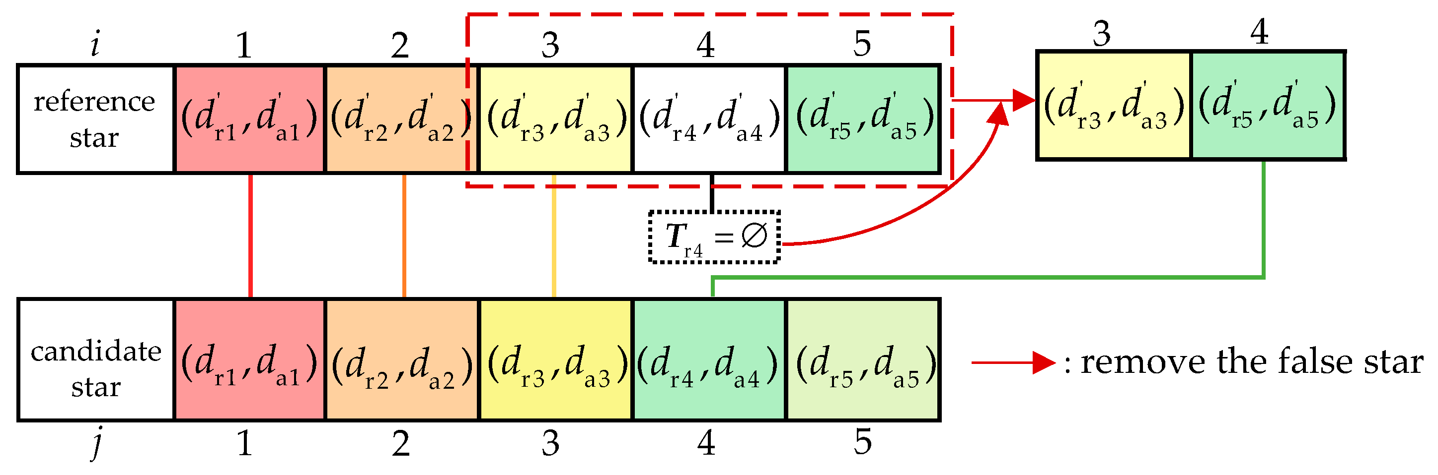
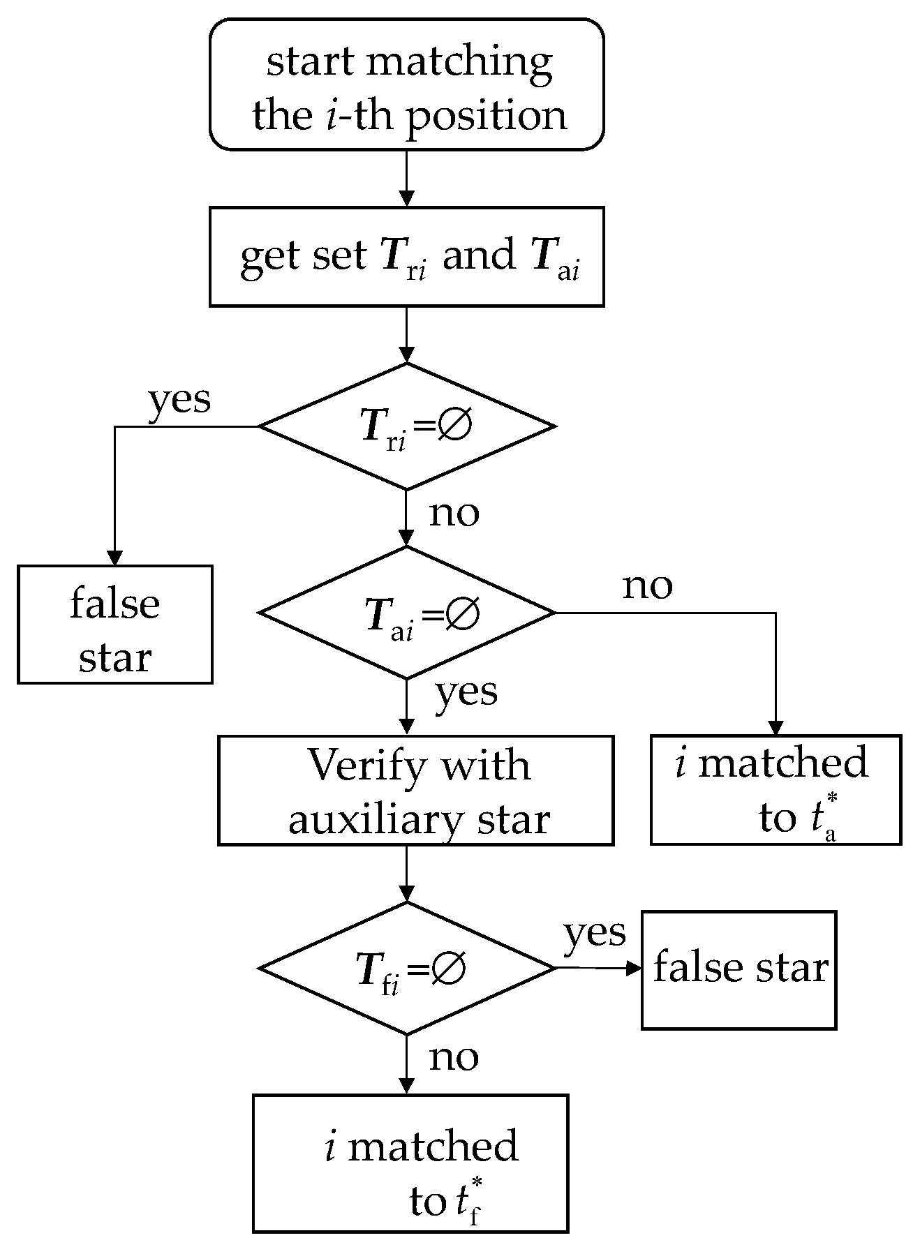
• If $T_{\mathrm{r}i}=\varnothing$, the star at the i-th position in the reference sequence is considered a false star. To preserve alignment for subsequent matching, the feature at this position is removed, and the algorithm proceeds to the next position (corresponding to $T_{\mathrm{r}4}=\varnothing$ in the example of Figure 6).

  Figure 6. Schematic of false star processing. The numbers 1 to 5 indicate the positions in the feature sequences. Identical colors denote matched positions between the reference and candidate sequences: the same shade of a color indicates a match in both radial and adjacency features, while different shades of the same color indicate a match in radial features only. The red dashed box highlights a false star to be removed, showing its original context.

  Figure 6. Schematic of false star processing. The numbers 1 to 5 indicate the positions in the feature sequences. Identical colors denote matched positions between the reference and candidate sequences: the same shade of a color indicates a match in both radial and adjacency features, while different shades of the same color indicate a match in radial features only. The red dashed box highlights a false star to be removed, showing its original context.
• If $T_{\mathrm{r}i}\ne \varnothing$ and $T_{\mathrm{a}i}\ne \varnothing$, the index $t\in T_{\mathrm{a}i}$ that minimizes $\left|d_{\mathrm{r}t}-d_{\mathrm{r}i}^{\prime }\right|+\left|d_{\mathrm{a}t}-d_{\mathrm{a}i}^{\prime }\right|$ is selected and denoted as $t_{\mathrm{a}}^{*}$. The star at the i-th position in the reference sequence is then matched to the star at the $t_{\mathrm{a}}^{*}$-th position in the candidate sequence.
• If $T_{\mathrm{r}i}\ne \varnothing$ but $T_{\mathrm{a}i}=\varnothing$, the star at the i-th position in the reference sequence is potentially matched to a star with an index in $T_{\mathrm{r}i}$. Further verification is then performed using the auxiliary star corresponding to the feature position pair (u,v) obtained during initial matching.

Invariant Angular Distance Verification with Auxiliary Stars

In Case 3, where the radial feature matches but the adjacency feature does not meet the threshold condition, the algorithm performs invariant angular distance verification using the auxiliary star for each candidate index in $T_{\mathrm{r}i}$ to avoid false matches.

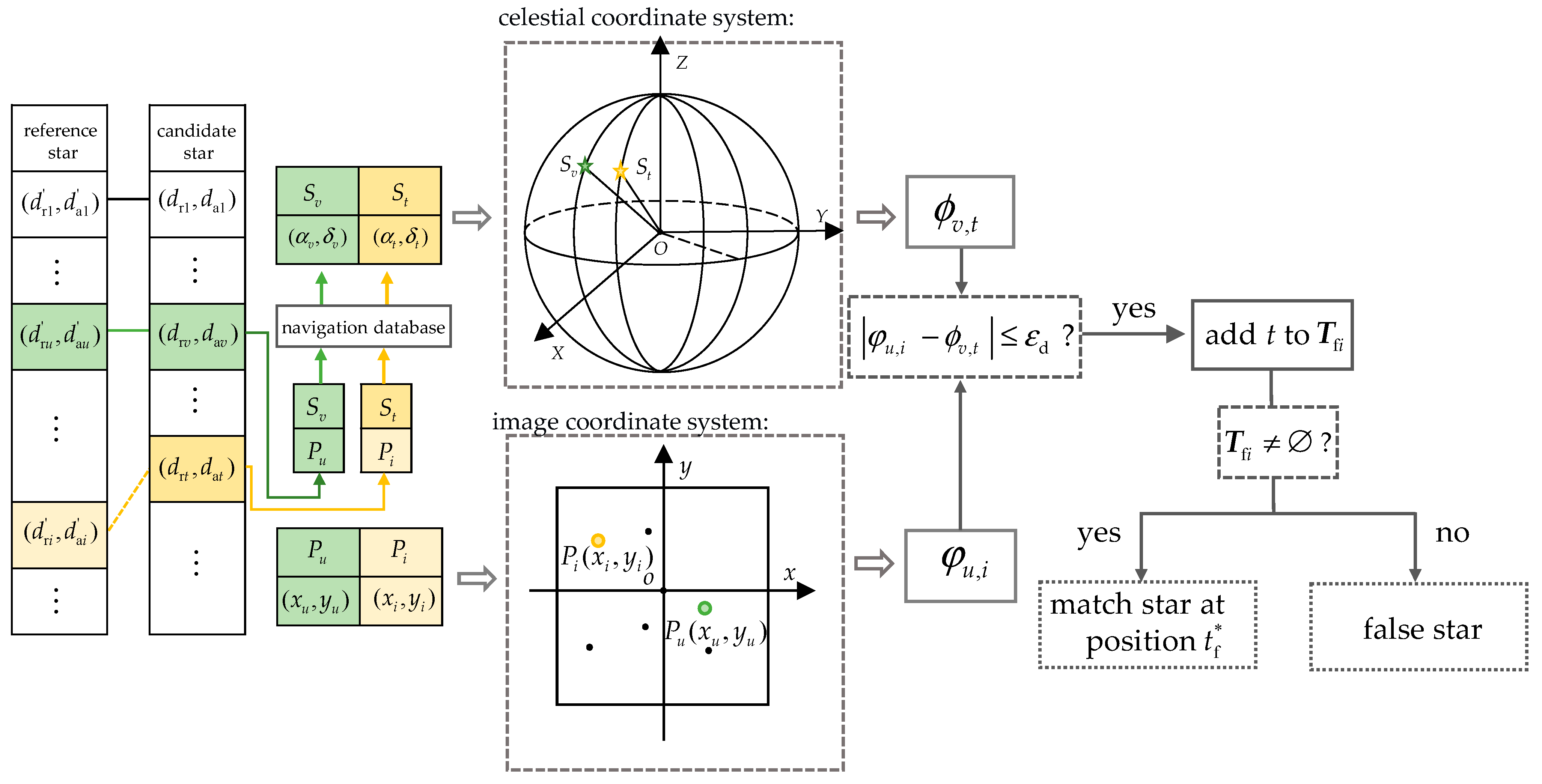
As shown in Figure 7, for each index $t\in T_{\mathrm{r}i}$, the right ascension and declination of the neighboring star $S_t$, denoted as $({\alpha }_t,{\delta }_t)$, are retrieved from the navigation database. Meanwhile, the right ascension and declination of the auxiliary star $S_v$, denoted as $({\alpha }_v,{\delta }_v)$, are also obtained. Their spherical angular distance ${\varphi }_{v,t }$ is then calculated using Equation (3). Simultaneously, the image coordinates $(x_u,y_u)$ and $(x_i,y_i)$ of the corresponding neighboring stars are extracted from the star image, and their observed angular distance ${\phi }_{u,i }$ is computed via Equation (4).

If the difference between the two angular distances satisfies the threshold condition

$$\left|{\varphi }_{v,t }-{\phi }_{u,i }\right|\le {\epsilon }_{\mathrm{d}},$$

(10)

The index t passes the verification. All indices that pass verification form the set $T_{\mathrm{f}i}$. If $T_{\mathrm{f}i}\ne \varnothing$, the index $t_{\mathrm{f}}^{*}\in T_{\mathrm{f}i}$ that minimizes the sum of the absolute radial feature deviation and the absolute auxiliary angular distance deviation is selected. The star at the i-th position in the reference sequence is then confirmed to match the star at the $t_{\mathrm{f}}^{*}$-th position in the candidate sequence. If $T_{\mathrm{f}i}=\varnothing$, the star at the i-th position in the reference sequence is considered a false star and removed from the sequence. This dual-verification mechanism effectively prevents false matches, thereby significantly enhancing the algorithm’s robustness.

To preserve positional correspondence, once the feature at reference position i is matched with that at candidate position j, the next reference feature at position i + 1 is compared with candidate features starting from position j + 1. The process terminates when i > m or j > n. The total number of successfully matched feature pairs is recorded as the matching score N_match, which quantifies the similarity between the feature sequences of the reference and candidate stars.

Robustness to False and Missing Stars

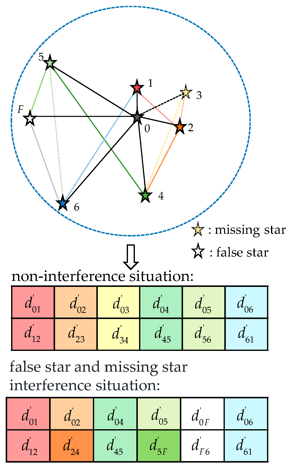
As illustrated in Figure 8, in practical star images, false or missing stars disrupt the sequential correspondence between the reference and correct navigation feature sequences by introducing extra elements or causing omissions. Additionally, such a star alters the adjacency feature of its preceding feature neighbor, but the radial feature of that neighbor remains unaffected.

To address the aforementioned impacts caused by false or missing stars—namely, the misalignment of the feature sequence and the alteration of a preceding feature neighbor’s adjacency feature—the algorithm employs local search matching combined with auxiliary star verification, as illustrated in Figure 9. First, through local search, the algorithm obtains the radial match set $T_{\mathrm{r}i}$ and the adjacency match set $T_{\mathrm{a}i}$ for the current feature of the reference star. If $T_{\mathrm{r}i}=\varnothing$, the star is considered a false star and is directly removed, thereby resolving the sequence misalignment caused by the false star. If $T_{\mathrm{r}i}\ne \varnothing$ and $T_{\mathrm{a}i}=\varnothing$, the star may be a preceding feature neighbor affected by a false or missing star. In this case, the algorithm performs angular distance invariance verification for each candidate position in $T_{\mathrm{r}i}$ based on the auxiliary star, and the positions that pass verification form the set $T_{\mathrm{f}i}$. If $T_{\mathrm{f}i}\ne \varnothing$, the optimal match is selected from it, allowing the star to be correctly identified despite the interference. Through the above mechanism, the algorithm effectively handles the impacts of false and missing stars.

2.2.4. Overall Star Identification Workflow

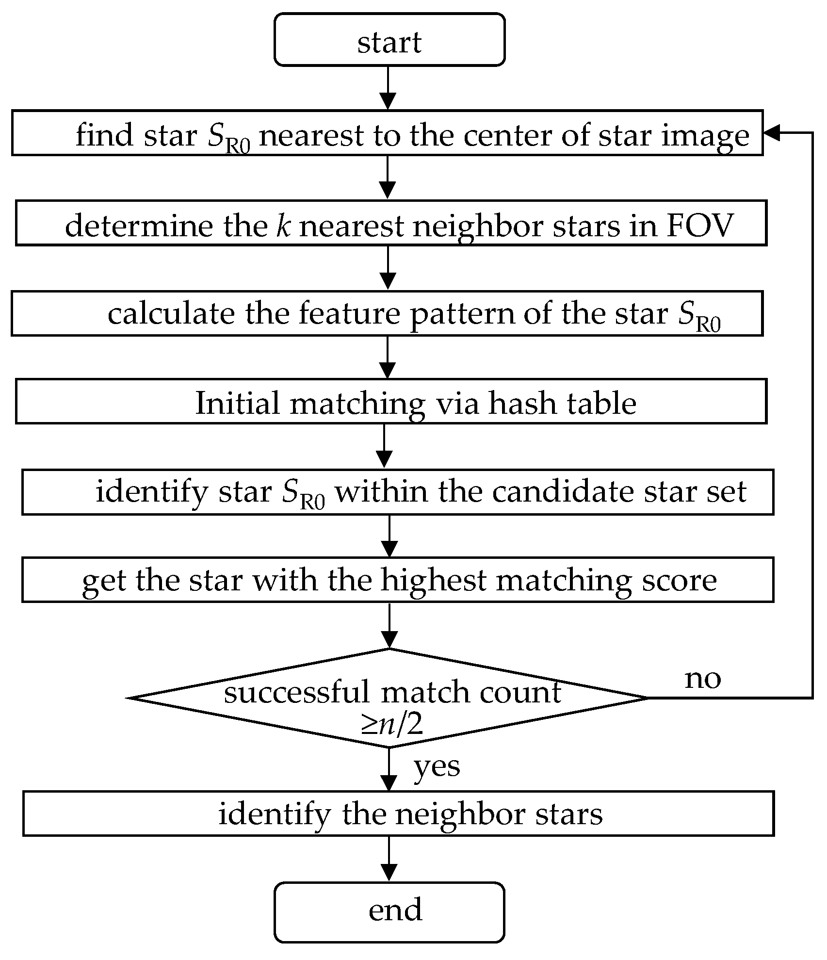
As shown in Figure 10, the overall star identification workflow is as follows. First, using the method described in Section 2.2.1, pattern features are extracted from the star image for the reference star. Then, an initial matching step based on a hash table and binary search is performed to quickly filter a set of candidate navigation stars, thereby reducing the number of stars that require detailed matching. Next, feature matching is carried out for each candidate star. While calculating the match score for each feature position, if the cumulative number of feature positions with zero scores exceeds $m/2$ (where $m$ denotes the feature dimension of the reference star), the matching process for the current candidate star is terminated early.

After iterating through all candidate stars, the one with the highest matching score is selected. If multiple candidate stars share the highest score, that with the shortest feature length is chosen as the final match. Finally, the algorithm verifies whether this highest score is greater than or equal to $n/2$ (where $n$ denotes the feature dimension of the candidate star). If the threshold is met, the reference star is considered successfully identified, and the algorithm proceeds to identify its neighbor stars based on the indices stored in the navigation database. Otherwise, the identification fails, and the algorithm returns to the start to select a new reference star.

3. Implements and Results

The performance of the proposed algorithm is evaluated through comprehensive simulations and real star image tests. The simulation experiments have three objectives: to demonstrate the algorithm’s applicability across different sensor configurations, to determine the optimal value for the key parameter k, and to verify its robustness against position noise, magnitude noise, and false stars in comparison with established reference algorithms. Finally, the algorithm’s effectiveness is validated using real captured star images.

3.1. Simulation Experiment Validation

To evaluate the performance of the proposed algorithm, simulation experiments were conducted based on the 2MASS star catalog. Simulated star images with random boresight orientations were generated using Monte Carlo method on the PyCharm 2024.1.4 platform. All experiments were completed on a computer equipped with an Intel Core i5-12490F processor with a base frequency of 3.7 GHz. The simulation experiments incorporate three primary types of error:

• Position noise: imperfections in the star sensor’s optical system—such as optical distortion, principal point offset, focal length error, and star spot deformation due to image noise or motion blur—lead to deviations in the measured star centroid positions. To simulate these deviations, Gaussian noise with zero mean and standard deviations ranging from 0 to 2 pixels in increments of 0.5 pixels was added to both the x and y coordinates of each star in the simulated images. This range comprehensively considers the effects of optical system calibration errors, detector readout noise, dark current noise, and the stripe non-uniformity specific to short-wave infrared detectors on centroid localization. By applying gradually increasing noise levels, the simulation systematically evaluates algorithm performance from ideal conditions to scenarios with significant interference.
• Magnitude noise: during star sensor imaging, error sources such as stray light and inherent sensor limitations introduce inaccuracies in the measured intensity of starlight. To simulate this effect, Gaussian noise with zero mean and standard deviations ranging from 0 to 0.3 mag in increments of 0.05 mag was added to the instrumental magnitude of each star in the simulated images. This range is derived from the theoretical relationship between magnitude measurement error and signal-to-noise ratio, taking into account the noise characteristics of short-wave infrared InGaAs sensors and fluctuations in atmospheric background radiation. The gradually increasing noise levels enable a comprehensive evaluation of the algorithm’s robustness across varying interference intensities.
• False star interference: during star sensor imaging, false stars (pseudo-stellar objects) may appear in the star image due to planets, variable stars, stray light within the FOV, or defective pixels. To simulate this interference, six sets of experiments were conducted, and a specific percentage of false stars (relative to the number of true stars) was introduced into each set, with the percentage increasing from 0% to 50% in increments of 10%. All false stars were within the detectable magnitude range of the sensor.

3.1.1. Performance Under Varying FOV and Magnitude Limit

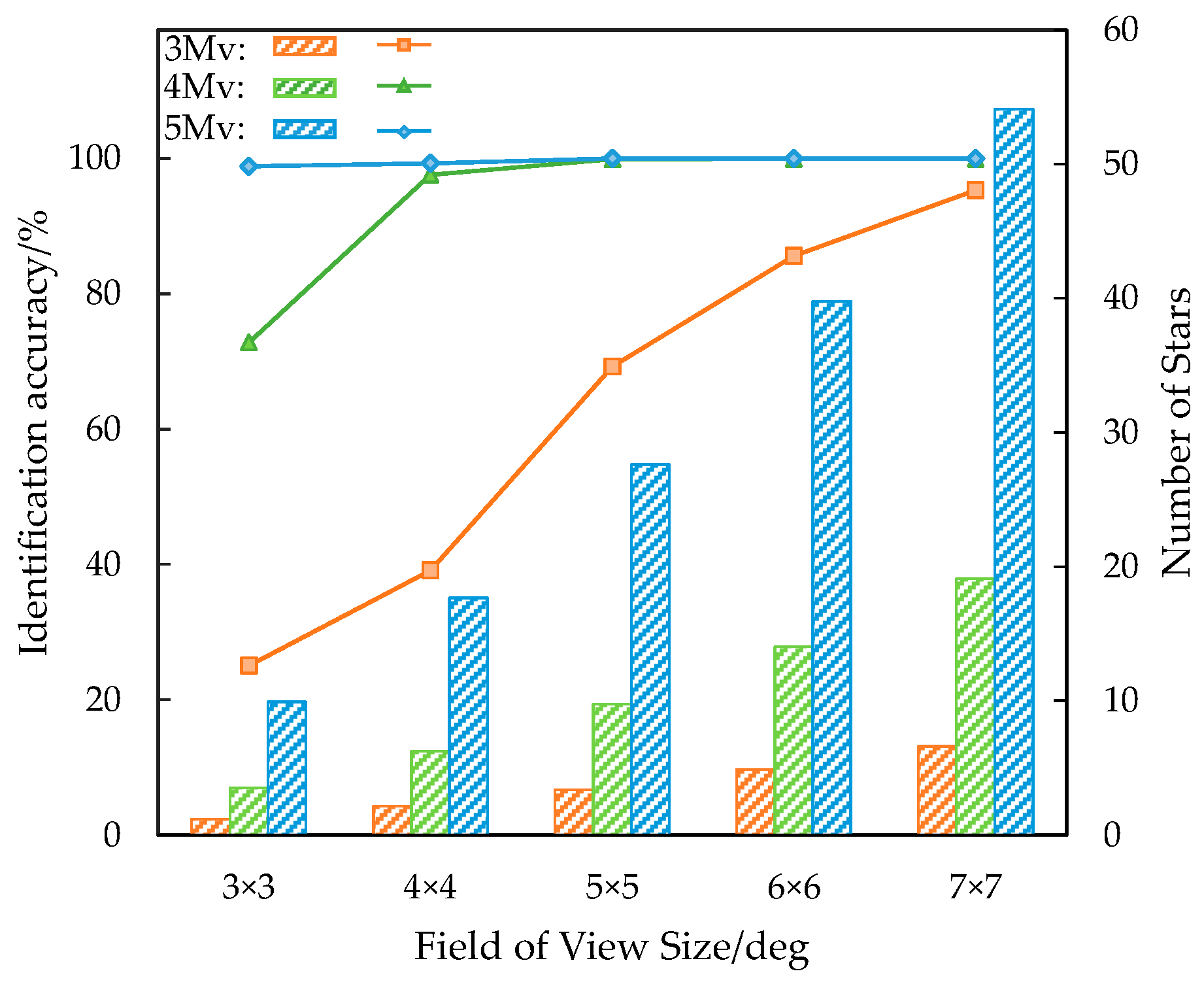
Simulation experiments were conducted to assess the algorithm’s adaptability to different sensor configurations by examining the effects of limiting magnitude and FOV. Three limiting magnitudes were tested: 3 Mv, 4 Mv, and 5 Mv. For each, the FOV was increased from $3^{\circ }\times 3^{\circ }$ to $7^{\circ }\times 7^{\circ }$ in steps. For each resulting parameter combination, the average number of stars within the FOV was calculated, and 5000 simulated star images with random boresight orientations were generated. The proposed algorithm was applied to these images, and its identification accuracy was statistically evaluated.

As shown in Figure 11, an increase in the FOV and limiting magnitude results in a greater average number of stars within the FOV, which is accompanied by an improvement in the identification accuracy of the proposed algorithm. Specifically, for an FOV of $4^{°}\times 4^{°}$ and a limiting magnitude of 4 Mv, the average number of stars is 6.25, corresponding to an identification accuracy of 97.62%. When the average number of stars increases to 9.76, the accuracy reaches 99.90%. These results demonstrate that the proposed algorithm is not only effective in narrow FOV with fewer stars but also maintains robust performance in wide FOVs with a greater number of stars.

3.1.2. Parameter Selection Analysis for the Number of Nearest Neighbors

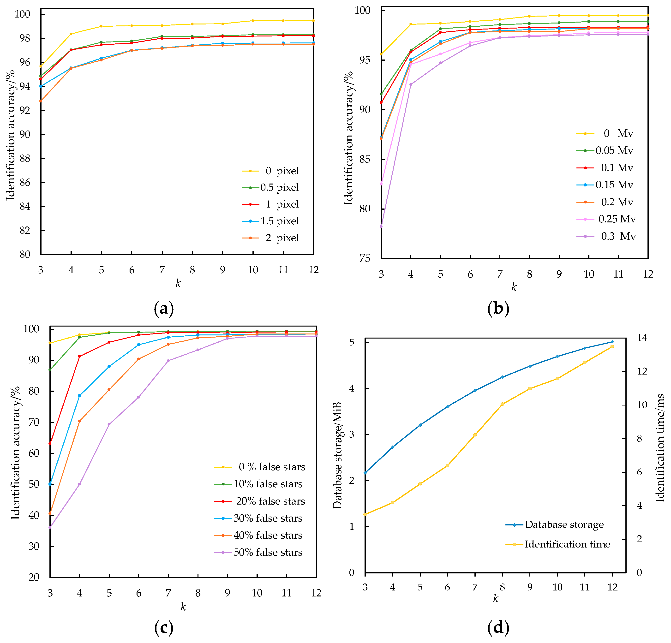
The FOV and limiting magnitude were fixed at ${4.312}^{\circ }\times {4.312}^{\circ }$ and 4 Mv, respectively, resulting in an average of 6.48 stars per image. To determine the optimal value for the key parameter ($k$, the number of nearest neighbors), experiments were conducted under three typical types of noise. For each intensity level of the three noise types (position error, magnitude error, and false star interference), a test set of 5000 simulated star images with random boresight orientations was generated. The algorithm’s identification accuracy was then evaluated across these test sets by systematically varying k. In addition, the navigation database memory usage and the average identification time per star image were recorded as functions of k.

As shown in Figure 12, under different noise disturbances, the identification accuracy first increases significantly and then gradually levels off as the number of neighboring stars k increases. When k is small, the feature pattern dimension is insufficient, making the algorithm susceptible to noise interference. As $k$ increases to 7–10, the uniqueness of the constructed star pattern features is enhanced, leading to a notable improvement in the robustness of the algorithm. When $k$ is further increased (11–12), the improvement in identification performance tends to plateau. Concurrently, both the identification time per frame and the navigation database storage increase with k. Balancing identification accuracy, computational efficiency, and storage overhead, $k=10$ is selected as the optimal parameter value.

In practical applications, the selection of parameters for different sensor configurations should follow a systematic approach: under the expected noise conditions (including position error, magnitude error, and false star ratio), the variation of identification accuracy with k is analyzed through simulated star images, and the smallest k value at which the identification accuracy plateaus while the computational cost remains acceptable is selected. This strategy ensures that the value of k is appropriately matched to the specific sensor characteristics and operational environment.

3.1.3. Performance Under Different Noise

To comprehensively evaluate the performance of the proposed algorithm, this section presents a comparative analysis between the proposed algorithm and five representative star identification algorithms under noisy conditions, with the optimal parameter k = 10. The selected algorithms cover different technical approaches: the triangle algorithm [15] and the grid algorithm [17] are widely adopted as classical baseline methods in practical engineering applications, serving to assess fundamental performance; the pyramid algorithm [16], as a geometry-based algorithm that has demonstrated strong robustness in recent studies, is employed to evaluate algorithmic stability under complex interference; the dynamic angle matching (DAM) algorithm [20] is included for comparison due to its conceptual similarity to the proposed algorithm and its proven robustness; in addition, to align with current research frontiers, an end-to-end deep learning-based star identification algorithm [22] is also included for comparison.

For each intensity level of the three noise types (position error, magnitude error, and false star interference), a test set of 5000 simulated star images with random boresight orientations was generated. The identification accuracy of all six algorithms was then evaluated and compared for each test set.

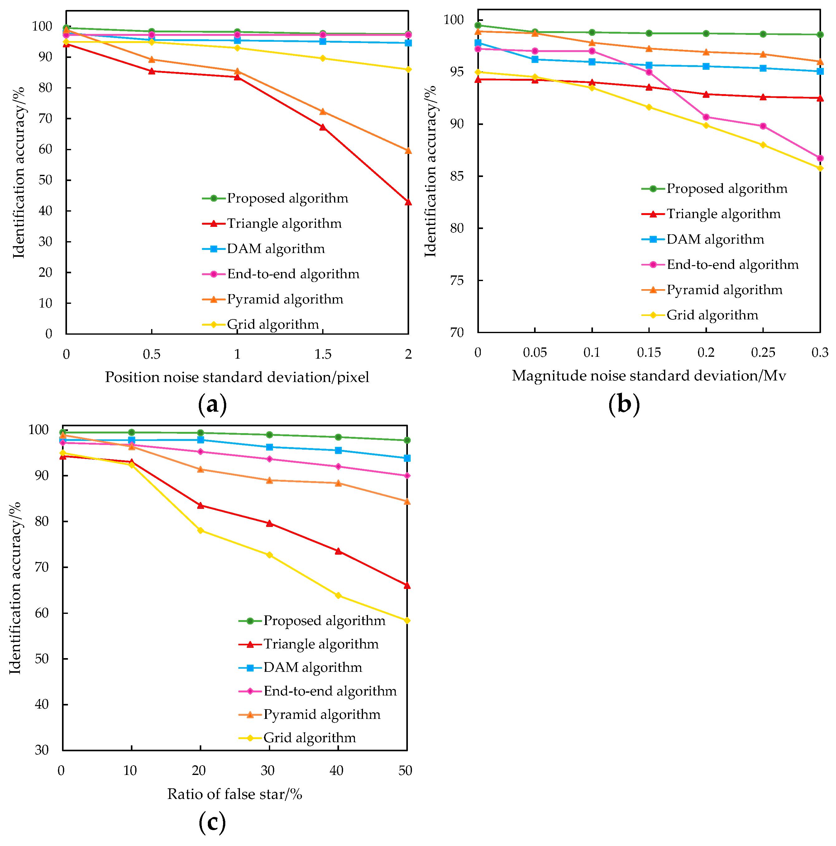
As shown in Figure 13, the performance of all six identification algorithms degrades to varying degrees as the noise intensity increases.

Figure 13a shows the performance under position noise. At the maximum noise level of 2 pixels, the triangle algorithm and the pyramid algorithm exhibit the most significant degradation, with their accuracy dropping to 42.92% and 59.62%, respectively. The grid algorithm achieves an accuracy of 85.96%, and the DAM algorithm reaches 94.56%. In contrast, under the same noise conditions, the proposed algorithm maintains an identification accuracy of 97.52%, which is comparable to that of the end-to-end algorithm (97.22%) and significantly outperforms the other methods, demonstrating strong robustness to star centroid deviations.

Figure 13b presents the results under magnitude noise. When the magnitude noise standard deviation reaches 0.3 Mv, the grid algorithm declines to 85.78%. The end-to-end algorithm also drops to 86.74%. In contrast, the triangle algorithm and the pyramid algorithm maintain relatively high accuracy levels of 92.52% and 96.02%, respectively. Under the same conditions, the proposed method achieves an identification accuracy of 98.60%, demonstrating strong robustness against magnitude noise.

Figure 13c illustrates the performance under false star interference. As the proportion of false stars increases from 0% to 50%, the triangle algorithm and the pyramid algorithm exhibit gradually decreasing accuracy, falling to 66.10% and 84.42%, respectively, at the maximum false star ratio. The grid algorithm, which relies on binary encoding of star patterns, is most vulnerable to false star interference, with its accuracy dropping to 58.38%. The proposed algorithm maintains the highest accuracy throughout, reaching 97.76% under the same condition.

3.1.4. Performance Comparison Under Combined Noise Interference

The memory usage of the star sensor’s navigation database directly impacts spacecraft storage and resource allocation, while the efficiency of the star identification algorithm is critical for real-time attitude determination. To comprehensively evaluate algorithm performance, simulated star images were generated incorporating combined interference: position noise (zero mean, standard deviation of 1 pixel), magnitude noise (zero mean, standard deviation of 0.15 Mv), and a false star ratio of 30%. Using this combined noise configuration, 5000 simulated star images with random boresight orientations were generated. All six algorithms were applied to this dataset, and the following metrics were recorded for each: average identification time per image, identification accuracy, and navigation database memory usage. The results are presented in

Table 2. Performance comparison of six algorithms.

Technique	Identification Accuracy/%	Average Time/ms	Database Storage /MiB
Grid Algorithm	70.36	27.01	1.21
Triangle Algorithm	80.72	30.39	11.34
Pyramid Algorithm	84.64	44.52	11.34
DAM Algorithm	95.20	179.82	2.59
End-to-end Algorithm	92.06	132.87	32.22
Proposed Algorithm	96.12	10.57	4.70

.

3.2. Field Experiment Validation

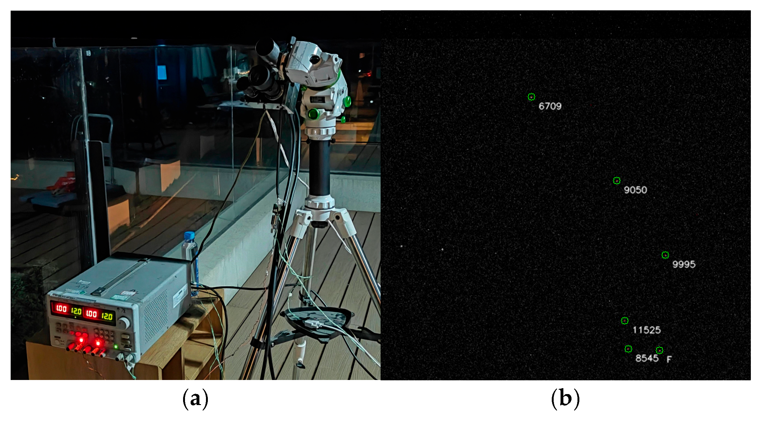
To validate the practical performance of the algorithm, field experiments were conducted at an open-air site in Guanshan Pasture, Baoji City, Shaanxi Province, China (elevation approximately 2200 m). The experiments were carried out under clear weather conditions with a visibility of approximately 30 km and a temperature of around 20 °C. The experimental setup consisted of an InGaAs SWIR camera (Figure 14a), the key specifications of which are listed in

Table 3. Camera parameters.

Parameter	Value
FOV/°	4.312 × 4.312
Array Size/pixel	512 × 512
Pixel Size/μm	15 × 15
Focal Length/mm	102
F-number/-	1.4
Sensor Model	A976515M1-B

.

From the captured star images, 97 frames containing at least four detectable stars were selected for testing, yielding an identification accuracy of 95.88%. This result validates the effectiveness of the proposed algorithm under actual observation conditions. A specific example is shown in Figure 14b: for the selected reference star within its field of view, five neighboring stars (including one false star) were detected, four of which were correctly identified.

4. Discussion

4.1. Analysis of Position Noise Results

Under the influence of position noise (Figure 13a), the triangle algorithm and the pyramid algorithm exhibit a significant decline in identification accuracy. This decline is primarily attributable to their reliance on precise angular distance matching in large-scale navigation star catalogs, where the angular distance tolerance must be set relatively tight to control redundant matches. When position noise causes the measured angular distances between observed stars to deviate from their theoretical values, true matching star pairs are excluded as they fall outside the tolerance range, leading to identification failure. Although the pyramid algorithm extends the matching primitive from three to four stars to increase feature dimensionality, it remains sensitive to position noise under a tight tolerance threshold. The grid algorithm suffers from encoding errors caused by star centroid shifts, with its identification accuracy dropping to 85.96%. The DAM algorithm constructs higher-dimensional features; however, it inherently relies on the imaging coordinates of stars to build these features, which introduces a systematic bias relative to the catalog features. Consequently, the introduction of position noise compounds this inherent bias, further degrading its identification performance. The end-to-end star identification algorithm first extracts local features from star neighborhoods through convolutional layers and then integrates them into high-dimensional global feature vectors via a Transformer encoder, demonstrating robust performance under position noise with an identification accuracy maintained at 97.22%. At the maximum noise level, the proposed algorithm achieves an identification accuracy of 97.52%, exhibiting strong robustness to star centroid deviations. This advantage stems from its high-dimensional feature construction, which preserves matching uniqueness within a practical tolerance range.

4.2. Analysis of Magnitude Noise Results

As shown in Figure 13b, under magnitude noise, the grid algorithm exhibits a notable performance degradation, with its accuracy dropping to 85.78% at a magnitude noise standard deviation of 0.3 Mv. This decline is primarily attributed to star loss or spurious stars caused by magnitude noise, leading to errors in nearest neighbor selection and subsequent identification failure. At the same noise level, the end-to-end algorithm also experiences a significant performance decline, with its accuracy falling to 86.74%. This is primarily because severe magnitude noise results in substantial loss of detectable stars, disrupting the inherent spatial structure of the star image and introducing deviations in the extracted global features. In contrast, the triangle algorithm and the pyramid algorithm demonstrate strong robustness, benefiting from the verification mechanism embedded in their identification strategies: if the currently selected stars fail to yield a valid match or produce redundant matches due to noise, the combination is automatically discarded and alternative stars are reselected for identification. Compared with the other algorithms, the proposed method maintains an identification accuracy above 98.60% under the same magnitude noise conditions, exhibiting strong robustness against magnitude noise. This advantage stems from its local search matching mechanism, which preserves the positional correspondence between the reference star and the correct navigation star feature sequence even in the presence of false or missing stars caused by magnitude errors, thereby ensuring accurate identification.

4.3. Analysis of False Star Interference Results

As shown in Figure 13c, under increasing proportions of false stars, the identification accuracy of all evaluated algorithms declines. The triangle algorithm and the pyramid algorithm are susceptible to misidentification due to erroneous feature patterns introduced by false stars, while the grid algorithm suffers from encoding errors, leading to a notable performance degradation. In contrast, the proposed algorithm demonstrates strong robustness against false star interference by handling two distinct scenarios. When a true star serves as the reference star, false stars may appear among its neighbors, disrupting the original neighborhood feature structure. To mitigate this issue, the algorithm incorporates an angular distance invariance verification during local search matching: if the radial feature matches but the adjacency feature does not, the candidate position is further verified using an auxiliary star. This mechanism enables the algorithm to filter out false star interference while still correctly identifying affected neighboring stars. When a false star itself is selected as the reference star, the algorithm applies a matching validity verification to exclude it. Specifically, the number of successfully matched feature pairs is counted. If this count reaches or exceeds half the feature dimension of the candidate star (i.e., n/2), the reference star is deemed successfully identified; otherwise, identification is deemed failed and another star is reselected as the reference. This mechanism effectively prevents misidentification caused by false stars, whether they appear as neighbors or as the reference star itself.

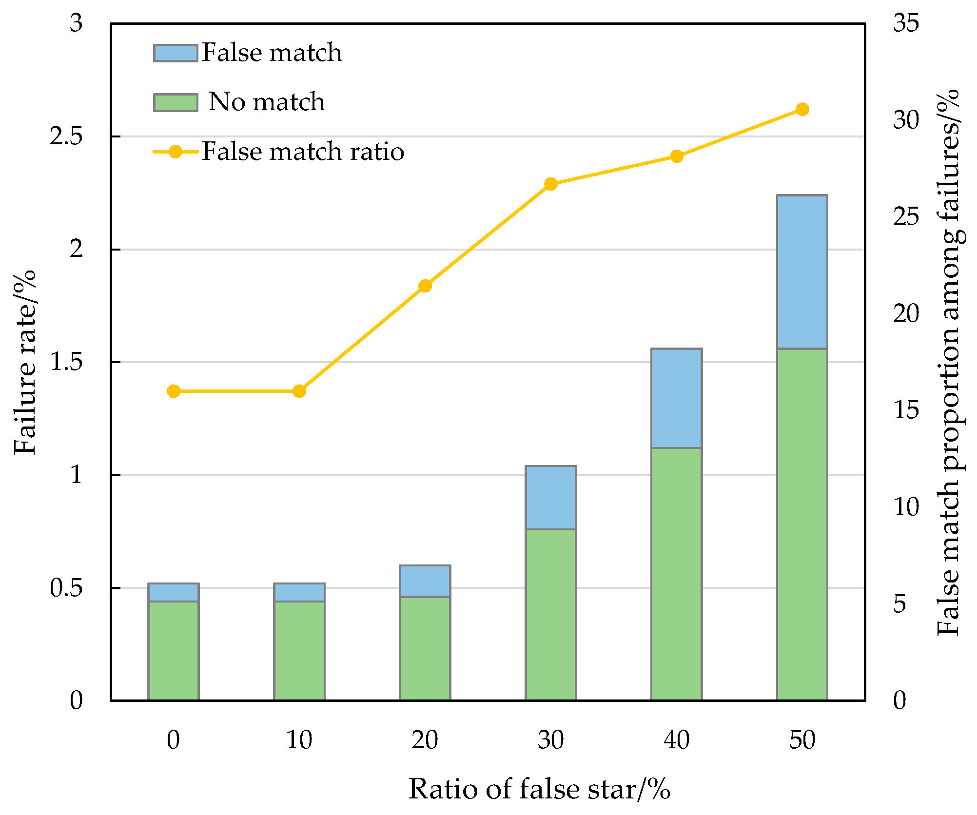
To quantitatively evaluate the effectiveness of these mechanisms in suppressing false matches, the proportion of false matches among identification failures is further analyzed. As shown in Figure 15, this proportion increases gradually with the false star ratio. Nevertheless, it remains below 31% across all tested conditions, demonstrating that the algorithm effectively limits false matches to a low level even under increasing false star interference, thereby preventing erroneous attitude determination.

4.4. Comprehensive Performance Analysis

As shown in Table 2, under combined noise interference, the triangle algorithm and the pyramid algorithm exhibit poor identification performance due to their sensitivity to position noise. Similarly, the grid algorithm suffers a significant drop in accuracy, as noise interference leads to encoding errors. The end-to-end algorithm is sensitive to star loss and thus performs poorly in the presence of magnitude noise. In contrast, both the proposed algorithm and the DAM algorithm demonstrate strong robustness, owing to their well-designed adaptive mechanisms. However, the DAM algorithm requires 179.82 ms per frame for identification, which limits its real-time applicability. The proposed algorithm achieves a much lower processing time of only 10.57 ms per frame. This efficiency gain is primarily attributed to the fast initial matching implemented via a hash table based on quantized features, which substantially reduces the number of navigation stars requiring subsequent detailed matching. In terms of storage overhead, the navigation database of the proposed algorithm occupies a relatively larger space due to the construction of the hash table. Experimental results indicate that the proposed algorithm achieves an effective balance among identification accuracy, computational efficiency, and storage requirements.

4.5. Limitations and Future Work

While the proposed algorithm exhibits robustness against various types of noise interference, a thorough analysis of its limitations and the experimental design is necessary for an objective evaluation of its practical applicability and for identifying future directions for improvement.

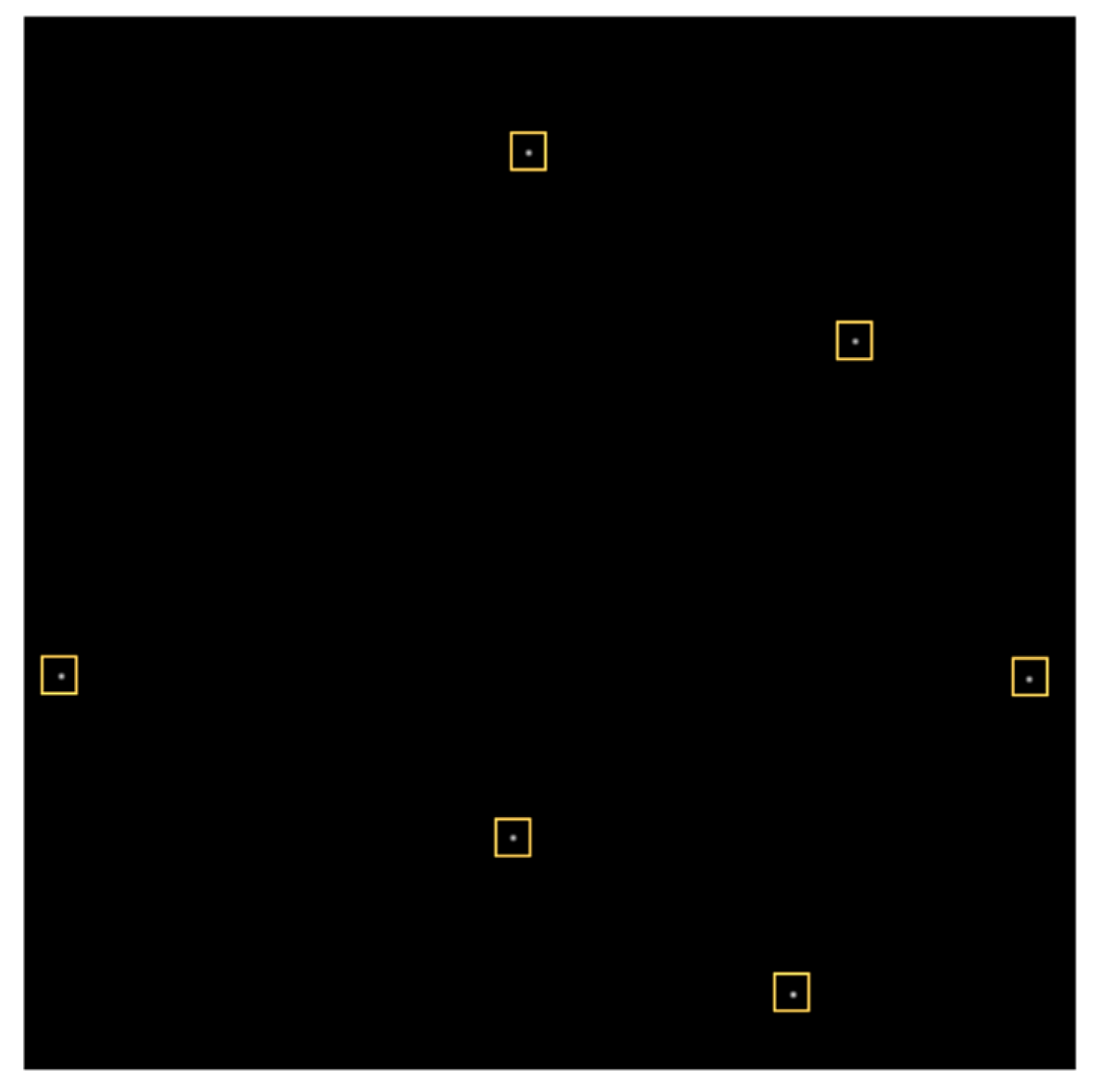
Under ideal simulation conditions, the algorithm achieves an identification accuracy of 99.48%, corresponding to a failure rate of 0.52%. Analysis of the failed star images reveals a common characteristic: the stars in these images are all located near the edge of the field of view, far from the image center. When a reference star is close to the field edge, its neighboring stars often fall outside the field of view, resulting in significant degradation of the feature vector. During the initial matching stage, the radial and adjacency feature pairs at each position in the feature sequence fail to match the corresponding feature pairs of the correct navigation star. As a result, the correct navigation star is excluded from the candidate set, ultimately causing identification failure. Figure 16 illustrates an example of such matching failures under ideal conditions. This finding reveals an inherent limitation of the current algorithm: the effectiveness of the initial matching mechanism depends, to some extent, on the integrity of the local star pattern around the reference star. When the reference star itself is located near the edge of the field of view, the number of available neighboring stars is inherently limited. Under such conditions, the algorithm may fail even in the absence of noise interference. It should be noted that, as the boresight orientations were generated using a Monte Carlo method, the probability of all stars being positioned at the field edge is extremely low; consequently, the practical impact of this limitation is minimal.

During field observations, the algorithm’s identification accuracy drops to 95.88%, compared to 99.48% achieved under ideal simulation conditions. This performance degradation can be attributed to several factors. First, when a reference star is located far from the field center, the integrity of its feature pattern is inherently compromised. If, in addition, defective pixels (which are characteristic of short-wave infrared detectors) appear within the reference star’s field of view, or if magnitude instability causes some observed stars to appear fainter than the 4 Mv limiting magnitude, the feature pattern is further degraded, ultimately resulting in identification failure.

Regarding the experimental design, the simulation validation in this study employed a Monte Carlo method with 5000 randomly generated boresight orientations. While this approach ensures statistical significance, it may not fully cover all regions of the celestial sphere, particularly those with extremely sparse star distributions. This limitation suggests that the algorithm’s performance in such sparse star fields requires further validation. Additionally, the scope of the field experiments is limited: the tests were conducted at a single location (Guanshan Pasture) under a single weather condition (clear weather), and only a limited number of valid star images were acquired. Therefore, the observed identification rate of 95.88% is insufficient to fully demonstrate the algorithm’s stability under more diverse observational conditions. More comprehensive evaluations (such as performance under different weather conditions, at different times, or in various observational environments) were not conducted due to the constraints inherent to ground-based observations.

In summary, future work will focus on the following aspects: optimizing the initial matching mechanism to enhance the algorithm’s adaptability when the reference star is located near the edge of the field of view; conducting larger-scale field experiments under more diverse conditions to accumulate a more extensive dataset of real star images and more comprehensively evaluate the algorithm’s practical performance; exploring more efficient simulation validation methods, such as full-sphere traversal tests, to further verify the algorithm’s applicability under different star distributions; obtaining precise noise models of the specific short-wave infrared sensor through laboratory calibration, thereby enabling more accurate simulation parameters for position and magnitude noise; and testing the algorithm on an embedded platform comparable to actual flight hardware to obtain a more accurate assessment of its runtime and real-time performance.

5. Conclusions

This paper proposes a two-stage star identification algorithm for infrared star images based on rotation-invariant features. After constructing radial and adjacency features from a sorted sequence of neighboring stars, the algorithm first employs a hash table for fast initial matching to generate candidate star sets, and then applies a local search procedure combined with auxiliary star verification to ensure reliable identification under complex interference. Experimental results show that the proposed algorithm outperforms several representative methods in both robustness and real-time performance, providing a practical solution for star identification in images with a limited number of stars.

References

1. Yi, J.; Ma, Y.; Long, H. On-orbit high-precision calibration for deep-coupled parameters of star sensor and gyroscope systems. Opt. Express 2024, 32, 32187–32209. [Google Scholar]
2. Ramos-Alcaraz, G.E.; Alonso-Arévalo, M.A.; Nuñez-Alfonso, J.M. Star-Identification System Based on Polygon Recognition. Aerospace 2023, 10, 748. [Google Scholar] [CrossRef] [Scilit]
3. Sun, T.; Yang, K.; Han, Y. Review of star identification algorithms under visible light conditions. Opt. Tech. 2023, 49, 469–475. [Google Scholar]
4. Wang, H.; Wang, B.; Gao, Y. Near-Earth space star map simulation method for short-wave infrared star sensors. Infrared Phys. Technol. 2022, 127, 10447. [Google Scholar] [CrossRef] [Scilit]
5. Wang, B.; Wang, H.; Mao, X. Optical system design method of near-earth short-wave infrared star sensor. IEEE Sens. J. 2022, 22, 22169–22178. [Google Scholar] [CrossRef] [Scilit]
6. Wang, W.; Wei, X.; Li, J. Noise suppression algorithm of short-wave infrared star image for daytime star sensor. Infrared Phys. Technol. 2017, 85, 382–394. [Google Scholar] [CrossRef] [Scilit]
7. Liao, Z.; Dong, Z.; Wang, H. Analysis of flow field aero-optical effects on the imaging by near-earth space all-time short-wave infrared star sensors. IEEE Sens. J. 2022, 22, 15044–15053. [Google Scholar] [CrossRef] [Scilit]
8. Wu, L.; Xu, Q.; Wang, H. Guide Star Selection for the Three-FOV Daytime Star Sensor. Sensors 2019, 19, 1457. [Google Scholar] [CrossRef] [Scilit]
9. Wang, W.; Wei, X.; Li, J. Optical Parameters Optimization for All-Time Star Sensor. Sensors 2019, 19, 2960. [Google Scholar] [CrossRef] [Scilit] [PubMed]
10. Yan, J.; Jiu, B.; Liu, H. Prior Knowledge-Based Simultaneous Multibeam Power Allocation Algorithm for Cognitive Multiple Targets Tracking in Clutter. IEEE Trans. Signal Process. 2014, 63, 512–527. [Google Scholar] [CrossRef] [Scilit]
11. Wang, W.; Wei, X.; Li, J. Guide star catalog generation for short-wave infrared (SWIR) All-Time star sensor. Rev. Sci. Instrum. 2018, 89, 075003. [Google Scholar] [CrossRef] [Scilit]
12. Parra, F.; Meza, P.; Torres, S.N. Modeling and compensating non-uniformity in push-broom NIR hyperspectral imaging system. Infrared Phys. Technol. 2014, 63, 204–210. [Google Scholar] [CrossRef] [Scilit]
13. Pan, Y.; Wang, H.; Jing, N. Parameter selection and optical design of all-day star sensor optical system. Acta Photonica Sin. 2016, 45, 157–163. [Google Scholar]
14. Liao, Y.; Zhang, L. A short-wave infrared star identification algorithm based on double features. Electron. Opt. Control 2024, 31, 56–61. [Google Scholar]
15. Liebe, C.C. Pattern recognition of star constellations for spacecraft applications. IEEE Aerosp. Electron. Syst. Mag. 2002, 8, 31–39. [Google Scholar] [CrossRef] [Scilit]
16. Mortari, D.; Samaan, M.A.; Bruccoleri, C. The pyramid star identification technique. Navigation 2004, 51, 171–183. [Google Scholar] [CrossRef] [Scilit]
17. Padgett, C.; Kreutz-Delgado, K. A grid algorithm for autonomous star identification. IEEE Trans. Aerosp. Electron. Syst. 1997, 33, 202–213. [Google Scholar] [CrossRef] [Scilit]
18. Xu, Y.; Zhang, Y.; Ye, Z. An improved grid algorithm based on angular distance feature for star identification. Navig. Position. Timing 2024, 11, 97–105. [Google Scholar]
19. Zhang, G.; Wei, X.; Jiang, J. Full-sky autonomous star identification based on radial and cyclic features of star pattern. Image Vision Comput. 2008, 26, 891–897. [Google Scholar] [CrossRef] [Scilit]
20. Sun, X.; Zhang, R.; Shi, C. Star identification algorithm based on dynamic angle matching. Acta Opt. Sin. 2021, 41, 1610001. [Google Scholar] [CrossRef] [Scilit]
21. Wang, H.; Wang, Z.; Wang, B. An artificial intelligence enhanced star identification algorithm. Front. Inf. Technol. Electron. Eng. 2020, 21, 1661–1670. [Google Scholar] [CrossRef] [Scilit]
22. Han, J.; Yang, X.; Xu, T. An End-to-End Identification Algorithm for Smearing Star Image. Remote Sens. 2021, 13, 4541. [Google Scholar] [CrossRef] [Scilit]
23. Yu, W.; Qu, H.; Zhang, Y. A high-accuracy star centroid extraction method based on Kalman filter for multi-exposure imaging star sensors. Sensors 2023, 23, 7823. [Google Scholar] [CrossRef] [Scilit]
24. Rijlaarsdam, D.; Yous, H.; Byrne, J. A survey of lost-in-space star identification algorithms since 2009. Sensors 2020, 20, 2579. [Google Scholar] [CrossRef] [Scilit] [PubMed]
25. Zheng, X.; Shen, J.; Wei, Z. Star map simulation and platform influence of airborne star sensor based on J-band data of 2MASS catalog. Infrared Phys. Technol. 2020, 111, 03541. [Google Scholar] [CrossRef] [Scilit]
26. Xing, F.; You, Z.; Sun, T. APS CMOS Star Sensor System: Principles and Implementation Methods; National Defense Industry Press: Beijing, China, 2017; pp. 128–129. [Google Scholar]
27. Gao, Y.; Zhao, J.; Chen, T. Radial neighbor feature with compensate code star pattern recognition algorithm. Opt. Precis. Eng. 2017, 25, 1627–1634. [Google Scholar] [CrossRef] [Scilit]
28. Wei, X.; Wen, D.; Song, Z. A star identification algorithm based on radial and dynamic cyclic features of star patterns. Adv. Space Res. 2019, 63, 2245–2259. [Google Scholar] [CrossRef] [Scilit]
Figure 1. Schematic of star sensor imaging model. Stars (red and green star symbols) represent real celestial objects, and their corresponding image points on the sensor plane are shown as circular dots of the same color.
Aerospace 13 00256 g001
Figure 2. Schematic of “edge loss”. Star symbols represent imaged star points. Blue stars are those successfully imaged within the FOV, while light-blue stars represent stars that fall outside the FOV and are lost. The arrow indicates the radius of the circular FOV, labeled as “FOV/2”.
Aerospace 13 00256 g002
Figure 3. Schematic diagram of the feature construction method: (a) Radial feature construction; (b) Adjacency feature construction. The central star labeled 0 represents the navigation star S 0 . The numbers 1 to 8 indicate the neighboring stars sorted in ascending order of angular distance from S 0 .
Aerospace 13 00256 g003
Figure 4. Impact of the edge loss on pattern features. The central star labeled 0 represents the navigation star S 0 . The numbers 1 to 8 indicate the neighboring stars sorted in ascending order of angular distance from S 0 . Solid lines represent successfully observed angular distances used for feature construction. Dashed lines represent angular distances that are lost due to edge stars falling outside the FOV.
Aerospace 13 00256 g004
Figure 5. Hash table construction. Blue highlights the processing flow of a radial feature value: quantization to a key, mapping to a hash bucket, and storage of the corresponding tuple.
Aerospace 13 00256 g005
Figure 7. Principle of auxiliary verification. Star symbols represent stars in the celestial coordinate system; circular dots represent their imaged points in the image coordinate system. Different colors (yellow and green) distinguish two stars, with the same colors used in the left feature sequences to indicate their corresponding entries. The two shades of yellow indicate a pending match. Solid lines denote established matches; dashed lines indicate the position to be verified. The question mark represents the decision condition.
Aerospace 13 00256 g007
Figure 8. Schematic of a star image affected by false and missing stars. The central star labeled 0 represents the reference star. The numbers 1 to 6 indicate the neighboring stars sorted in ascending order of angular distance from star 0. Solid lines represent observed angular distances. Dashed lines indicate angular distances that are missing due to missing stars.
Aerospace 13 00256 g008
Figure 9. Flowchart of the local search matching mechanism.
Aerospace 13 00256 g009
Figure 10. Flow chart for star image identification.
Aerospace 13 00256 g010
Figure 11. Identification accuracy of the algorithm under different magnitude limits and FOVs.
Aerospace 13 00256 g011
Figure 12. Algorithm performance under different k values: (a) Identification accuracy under position noise; (b) identification accuracy under magnitude noise; (c) identification accuracy under false star interference; (d) memory usage of the navigation database and average identification time per image.
Aerospace 13 00256 g012
Figure 13. Identification accuracy of six algorithms under different noise interference: (a) position noise; (b) magnitude noise; (c) false stars interference.
Aerospace 13 00256 g013
Figure 14. Field experiment: (a) Observation equipment; (b) Identification result of the star image.
Aerospace 13 00256 g014
Figure 15. Decomposition of identification failures under false star interference.
Aerospace 13 00256 g015
Figure 16. Example of identification failure under ideal conditions. The stars are enclosed in boxes to highlight their positions for better visibility.
Aerospace 13 00256 g016