


Abstract
The high cost of Computational Fluid Dynamics (CFD) limits coupled CFD/Computational Structural Dynamics (CSD) simulations of rotorcraft. This study develops a data-driven Reduced-Order Model (ROM) using Dynamic Mode Decomposition with Control (DMDc) to simultaneously predict lift, drag, and pitching-moment coefficients (Cl, Cd, and Cm) for an airfoil-flap system. Complete input degrees of freedom (complete-DOF inputs) comprise the plunge velocity, pitch, flap deflection, and time-varying Mach number. A sliding-window rolling strategy incorporates flow-field memory and enables independent long-horizon prediction without output feedback. Standard DMDc and Hankel-DMDc use identical CFD data. Reconstruction tests progress from a single primary motion to complete-DOF inputs, followed by independent complete-DOF prediction. For pitch-amplitude scaling factors λα = 0.6–1.5, neither model accumulates error or diverges over 1.2 s of continuous prediction. Two local ROMs cover Ma = 0.20–0.40 and Ma = 0.30–0.50. Interpolating their outputs within the overlap extends coverage to Ma = 0.20–0.50. The framework supports efficient unsteady sectional load prediction for conventional rotors and smart rotors with active trailing-edge flaps, providing a basis for future ROM/CSD coupling. Applicability limits, including deep dynamic stall, and potential applications are discussed.
1. Introduction
Helicopters, Electric Vertical Takeoff and Landing (eVTOL) aircraft, and other rotorcraft are used for applications such as low-altitude transport [1], search and rescue, and agriculture [2]. Rotorcraft rely on their rotors to generate lift and propulsive force. The rotors also provide the primary means of flight control. Rotor design, performance improvement, and the development of advanced configurations require accurate and efficient aerodynamic calculations. The missions, structures, and motions of rotorcraft produce strongly unsteady flows [3]. In steady forward flight, for example, asymmetric inflow over the rotating blades produces periodic unsteady aerodynamic loads. Elastic blade deformation can cause sectional plunge and pitch, and sections of a smart rotor within the active trailing-edge flap span also experience controlled flap deflection. The rotor moves with the airframe during maneuvers, further changing local inflow and motion. These conditions motivate the inclusion of sectional plunge, pitch, flap deflection, and a time-varying freestream as model inputs. Computational Fluid Dynamics (CFD) can resolve these flows, but its computational cost limits its use in simulations coupled with Computational Structural Dynamics (CSD), as well as in design optimization and active control. Efficient aerodynamic models generally follow two routes: (1) physics-based models with explicit expressions and (2) data-driven Reduced-Order Models (ROMs) constructed from CFD results [4,5]. Here, an efficient aerodynamic model computes loads for prescribed motion and inflow without solving the flow field again, reducing the load computation time relative to direct CFD.
Physics-based models with explicit expressions commonly include empirical models [6], frequency-domain models [7], and Rational Function Approximation (RFA) [8]. They are computationally efficient and have explicit mathematical forms. These features make them convenient to incorporate into structural equations [9]. Their formulations nevertheless rely on prescribed expressions, potential-flow assumptions, or empirical corrections. In implementations of the widely used Leishman–Beddoes (L-B) model [6], plunge can be represented solely through its contribution to the equivalent angle of attack. However, pure plunge and pure pitch can produce different pitching-moment responses even when they yield the same equivalent angle of attack over time. The equivalent angle of attack alone does not account for the separate effects of pitch rate and pitch acceleration on the pitching moment. These effects are included in Theodorsen’s unsteady thin-airfoil theory [7]. Myrtle and Friedmann were among the earliest to apply RFA to rotor unsteady aerodynamics. They first approximated the aerodynamic transfer function in the frequency domain. An inverse Laplace transform then yielded a time-domain state-space model [10]. Subsequent work by Patt, Liu, Padthe, and Chia extended RFA to time-varying freestream conditions, Gurney flaps, and vibration and noise control [11,12,13,14].
Advances in CFD, experimental techniques, and data science have made CFD datasets for training ROMs more accessible. These data have enabled researchers to construct ROMs from CFD results. Such models can reduce the computational cost of parameter studies, design optimization, and aeroelastic analysis. An aerodynamic ROM retains the dominant dynamics in a lower-dimensional representation, allowing for rapid reconstruction or prediction of flow fields or aerodynamic loads without repeatedly running CFD simulations. In the mid-to-late 1990s, Dowell [15] proposed representing high-dimensional flows using a small number of dominant modes. This was an early representative contribution to aerodynamic ROMs. Silva [16] used digital filtering to identify aerodynamic impulse responses and built a low-dimensional input–output model. These studies provided a basis for the early development of aerodynamic ROMs. Subsequent data-driven research on unsteady aerodynamics developed several major routes. These include the Surrogate-Based Recurrence Framework (SBRF), multiple-input/multiple-output (MIMO) state-space identification, and parameterized modeling across Mach numbers. More recent work has also examined sparse identification, neural networks, feature extraction, and flow-field prediction [4,5,17].
SBRF uses a surrogate model to predict the current aerodynamic loads from motion, inflow, and previous loads. The predicted loads are then fed back as inputs for the next step. Existing SBRF-based ROMs can be divided broadly into two groups. One retains Kriging as the mapping method. The other replaces Kriging with a nonlinear mapping model, such as a Radial Basis Function Neural Network (RBFNN). Glaz et al. developed a Kriging-based reference model in the SBRF line of research [18]. Its inputs covered coupled airfoil pitch and plunge motions together with time-varying freestream conditions. The model used output feedback to capture aerodynamic memory. Glaz et al. subsequently extended SBRF to dynamic stall and swept flows [19,20]. P. Liu et al. applied SBRF to dynamic-stall prediction for a wind turbine airfoil [21]. H. Liu et al. coupled an SBRF model with a two-dimensional airfoil structural model to analyze aeroelastic responses [22]. Li et al. constructed an SBRF ROM for mild dynamic stall. They emphasized that initialization with static aerodynamic loads reduces the initial error in recursive prediction [23]. Stradtner and Bekemeyer developed an SBRF-based unsteady ROM for performance and stability assessment of a three-dimensional wing [24]. Kou and Zhang developed a recurrent RBFNN ROM with output feedback. They used particle swarm optimization to improve its generalization [25].
MIMO state-space identification uses multiple input and output time series to identify low-dimensional state-evolution and output equations. The resulting model predicts several aerodynamic coefficients simultaneously from motion and inflow inputs. Huang et al. developed a nonlinear ROM using a finite Wiener-type cascade. The cascade combined a dynamic linear module with a static nonlinear module. Its predictive accuracy was tested using a two-dimensional (2D) airfoil flutter case [26]. Liu et al. extended a MIMO state-space ROM to a three-dimensional (3D) wing with a control surface. They used modal superposition to calculate the transonic aeroelastic response [27]. Huang et al. subsequently constructed a nonlinear state-space ROM. The model was used to analyze the transonic behavior of a 3D wing, and its results were compared with CFD [28]. Yang et al. also developed a nonlinear state-space ROM. They identified its linear component using the Eigensystem Realization Algorithm (ERA) [29]. This ROM was later used to construct a 2D airfoil aero-servo-elastic system for active control of transonic buffet [30]. Autoregressive models with exogenous inputs (ARX) have also been applied to ROM identification [31,32]. Kou and Zhang used an RBFNN to predict the nonlinear residual of an ARX model. The resulting ROM placed the ARX model and RBFNN in parallel [33].
Several approaches have been proposed to build ROMs that operate across a wide Mach number range. Two main approaches are weighted blending of local ROMs and parameterization by operating condition. Skujins and Cesnik [34] linearly interpolated the outputs of local ROMs. This provided a continuous transition between different Mach number ranges. Winter and Breitsamter [35] built several local ROMs and blended their outputs using fuzzy validity functions. They used the blended model to predict the flutter boundary of the AGARD 445.6 wing. Other researchers have treated the Mach number as a prescribed operating parameter in a ROM. They used data from several discrete Mach number conditions to train one parameterized model. Kou and Zhang [36] used a recurrent RBFNN, whereas Li et al. [37] used a Long Short-Term Memory (LSTM) network. Both prescribed the Mach number as a fixed operating parameter and obtained ROMs that span multiple Mach number conditions. In a related approach, Immordino et al. [38] treated the Mach number and mean angle of attack (AOA) as operating parameters. They interpolated the Volterra kernels for different conditions using a Fully Connected Neural Network (FCNN) or Gaussian Process Regression (GPR) and then constructed a ROM.
Beyond parameterized modeling, researchers have developed ROMs through sparse identification, neural networks, and methods for extracting flow features and predicting flow fields. Sun et al. used Sparse Identification of Nonlinear Dynamics with Control (SINDYc) to develop a ROM with explicit equations [39]. The scalar expression reported in that study, however, computes only one output [39]. Candon et al. used sparse Volterra kernels and nonlinear fluid oscillators to describe aerodynamic memory and transonic buffet dynamics [40,41,42]. Deep learning methods have also been applied to airfoil aerodynamic prediction and deep dynamic-stall modeling. These methods include Recurrent Neural Networks (RNNs), Convolutional Neural Networks (CNNs), and Kolmogorov–Arnold Gated Recurrent Networks (KA-GRNs) [43,44,45]. In addition, ROMs based on autoencoders and nonlinear invariant manifolds extract low-dimensional flow features. They have been used for both reconstruction and prediction of unsteady flow fields [46,47].
This study focuses on sectional loads on an airfoil-flap system undergoing motion in multiple degrees of freedom in a time-varying freestream, without reconstructing the full flow field. To predict lift, drag, and pitching moment coefficients simultaneously, this study uses Dynamic Mode Decomposition with Control (DMDc) to identify state evolution and the influence of external inputs from CFD data. Delay embedding and sliding-window recursion enable long-horizon prediction without output feedback. Studies combining Proper Orthogonal Decomposition (POD) and DMDc have applied these methods to 2D airfoil aerodynamic prediction, separated-flow control, and prediction of surface pressure on a 3D wing [48,49,50]. These studies show that DMDc can represent unsteady flows driven by external inputs. Most existing applications, however, concern flow-field prediction for fixed-wing configurations or specific control tasks.
Rotor unsteady aerodynamics involves multiple inputs, strong coupling, broad parameter ranges, multiple time scales, and strong dependence on the history of motion and inflow (here termed flow-field memory). Existing modeling approaches face several limitations. (1) The amount of data required by interpolation and surrogate models grows rapidly as the input dimension and parameter range increase. Their extrapolation errors are also difficult to control. (2) In SBRF models with output feedback, one-step errors can accumulate over time. This can cause prediction drift and other stability issues [51]. (3) Deep neural networks often have complex architectures and high training costs. They also commonly lack explicit physical constraints or stability guarantees. Their long-horizon predictions may therefore become nonphysical. (4) Many existing ROMs consider only a few motion degrees of freedom or assume fixed freestream conditions. To address these limitations, this study makes four contributions:
- An end-to-end DMDc-based model maps motion and freestream inputs to aerodynamic responses. It predicts multiple aerodynamic coefficients simultaneously.
- Complete-DOF inputs are defined for rotor unsteady aerodynamics. The input vector includes motion in multiple degrees of freedom and a time-varying freestream. Input delays and delay embedding of the system state represent flow-field memory.
- A sliding-window rolling prediction strategy is proposed without output feedback. It enables independent long-horizon prediction of aerodynamic loads.
- Local ROMs defined over overlapping parameter ranges are blended to extend the Mach number envelope. In the overlap, neither local ROM needs to extrapolate. This avoids introducing extrapolation error into the blending step.
2. DMDc-Based Reduced-Order Modeling Framework
The unsteady aerodynamic loads on the airfoil-flap system depend on its motion, the time-varying freestream, and the history of the flow field. This study models the main airfoil and trailing-edge flap as a discrete dynamical system driven jointly by motion and freestream inputs. Its outputs are the lift coefficients, drag coefficients, and pitching moment coefficients (Cl, Cd, and Cm). This system serves as the common basis for the DMDc models developed in the following sections. A general nonlinear discrete dynamical system can be written as:
where xk denotes the system state at discrete time k. uk and yk are the external input and aerodynamic output, respectively. Fq and Gy denote the state-evolution and output-mapping operators. In the aerodynamic setting, the nonlinear equations in Equation (1) represent the CFD solver based on the Navier–Stokes equations. The state vector xk contains discrete flow variables at each grid point, such as density, velocity components, and energy. Its dimension therefore scales with the number of grid points and defines the order of the Full-Order Model (FOM). Obtaining a resolved solution generally requires a large full-order state. This study identifies the system’s input–output relationship from CFD time series to construct an aerodynamic ROM. During prediction, the ROM computes aerodynamic coefficients from prescribed inputs without repeatedly solving the complete flow field. This substantially reduces the computational cost.
Unsteady flow depends strongly on its history, partly because of fluid inertia. Even under identical instantaneous motion and inflow conditions, different motion and inflow histories can lead to different aerodynamic loads. This study assembles the input samples into a delay vector uk. The model can then use information within the input window to capture flow-memory effects. To facilitate ROM/CSD coupling, the ROM uses the airfoil pitch angle, flap deflection angle, and freestream Mach number directly, without taking their time derivatives. The plunge input is the plunge velocity. This formulation is compatible with the CSD module in integrated helicopter aeroelastic analysis software. The CSD module can directly supply the inputs required for uk, while the ROM returns Cl, Cd, and Cm. During coupled analysis, the ROM avoids repeatedly solving the governing flow equations, substantially reducing computational cost.
2.1. Degrees of Freedom and Dynamical System Representation
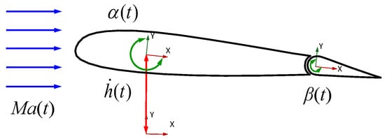
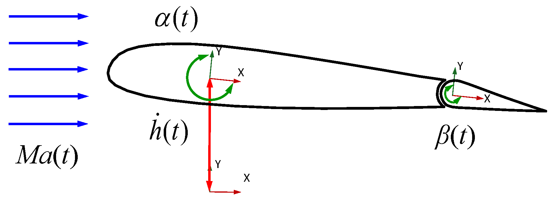
Figure 1 illustrates the complete-DOF inputs of the airfoil-flap system. They comprise plunge velocity , pitch angle α(t), flap-deflection angle β(t), and time-varying Mach number Ma(t). represents the instantaneous physical input vector of the airfoil-flap system.
Figure 1.
Complete-DOF inputs of the airfoil-flap system.
The drag coefficient Cd cannot be neglected in rotor aeroelastic analysis. Under realistic conditions, the aerodynamic coefficients are also coupled and subject to mutual constraints. Rather than constructing a separate ROM for each coefficient, this study combines Cl, Cd, and Cm into a single output vector. The three aerodynamic components are then identified and predicted simultaneously. This formulation is intended to improve the interpretability and deployment flexibility of the ROM. The output vector is expressed as:
let uk denote the instantaneous complete-DOF inputs at time tk. This study concatenates the current input with its preceding Nin samples to construct the input-delay vector uk:
where Nin denotes the input-delay order. The input history contained in uk enables DMDc to identify the system’s unsteady dynamics. This section combines the complete-DOF inputs and the three aerodynamic coefficient outputs into a unified input–output system. Section 2.2 briefly describes the construction of the DMDc ROMs.
2.2. DMDc-Based Reduced-Order Modeling
This study uses DMDc to identify low-dimensional aerodynamic models from the CFD-generated input–output time series. Standard DMDc serves as the baseline model. Hankel-DMDc extends this formulation by introducing output delay embedding. Both methods use the same motion inputs and aerodynamic outputs to ensure a consistent comparison.
2.2.1. Standard DMDc
Standard DMDc assumes that the system state and input vector satisfy the following state equation:
where A ∈ ℝn×n denotes the system state matrix, and B ∈ ℝn×l denotes the control matrix. xk ∈ ℝn×1 and uk ∈ ℝl×1 are the system state and input vectors, respectively. For Standard DMDc, the aerodynamic output is directly taken as the state, xk = y(tk). Here, the inputs are the prescribed motion and freestream quantities, and the outputs are the lift, drag, and pitching moment coefficients. The m state snapshots and corresponding input snapshots are assembled into the following matrices, taking the input delays into account:
where Nin denotes the input-delay order. According to Equation (4), the system matrices with inputs satisfy the following approximate relation:
where the matrices A and B provide the best fit to the snapshot data in Equations (5)–(7). The current-state snapshot matrix X and the lagged-input snapshot matrix Ƴ are stacked vertically. Singular value decomposition (SVD) is applied to the augmented matrix to identify the state and input matrices, with X′ as the fitting target. The algorithm for determining A and B is described in Ref. [52]. After identification, A and B remain fixed. The state is advanced at each step using Equation (4) and the corresponding delayed input. The resulting state gives the aerodynamic coefficients without rerunning CFD. The low-order model thus uses only input–output data to predict the loads rather than reconstructing the full flow-field state.
2.2.2. Hankel-DMDc
Standard DMDc constructs its state vector xk using only the current aerodynamic output. Unsteady flow exhibits pronounced memory effects and inertia. To represent this memory and the response lag of unsteady flow, Hankel-DMDc embeds the current output together with Nout preceding output samples into the system state vector:
where Nout denotes the output-delay embedding order. Following the Standard DMDc procedure in Section 2.2.1, consecutive states are used to construct the Hankel-state snapshot matrices. Applying the same augmented-matrix construction and singular value decomposition procedure gives:
where AH and BH denote the Hankel-state transition and control matrices, respectively. S is the output-selection matrix used to extract the aerodynamic coefficients at the latest time step from the delayed state. This formulation incorporates the history of aerodynamic load evolution into the system state without introducing additional input variables. By retaining past inputs and aerodynamic outputs, Hankel-DMDc implicitly represents the history dependence of unsteady flow.
2.3. Sliding-Window Rolling Prediction Strategy
Recursive models with output feedback, such as SBRF, are commonly used to model flow memory. In long-horizon autoregressive prediction, SBRF feeds the predicted output from the preceding time step back into the input. This may cause one-step errors to accumulate, leading to prediction drift or stability problems.
This study proposes a sliding-window rolling prediction strategy without output feedback to avoid these problems and SBRF’s dependence on prior data for initialization. Hankel delay embedding implicitly represents the historical-output information used by feedback models. The augmented state contains information from multiple time steps. Its internal evolution preserves temporal relationships in unsteady aerodynamic loads. The preceding predicted output therefore does not need to be explicitly fed back into the input. Thus, this strategy recasts SBRF’s dependence on historical outputs as the evolution of an augmented state.
The DMDc model has stable dynamics, as indicated by the eigenvalues of A. The influence of the initial value y(0) therefore decays rapidly, improving model applicability and robustness. For Hankel-DMDc, each predicted state contains aerodynamic information from several consecutive time steps. Each recursion extracts only the aerodynamic load at the latest time in the window as the output. The delay window then advances by one time step:
where the superscript denotes a ROM-predicted value, and the predicted output vector is defined as . This strategy performs step-by-step rolling prediction based on the delayed state. It does not predict an entire future signal in parallel at each time step. The model also requires no output feedback. The initial system state vector is set to zero at the start of prediction. Section 4.4 examines initial-condition decay, error accumulation, and long-horizon stability using independent-prediction results.
3. CFD Solutions
This study selects the NACA 23012 airfoil based on the BO105 rotor parameters. A moving overset mesh discretizes the computational domain. The far-field boundary is located 30 chord lengths c from the airfoil and 40 chord lengths c downstream in the wake region. The flow field is computed by solving the unsteady Reynolds-averaged Navier–Stokes (URANS) equations and the Spalart–Allmaras (S-A) turbulence model. Before the main simulations, mesh and time-step sensitivity tests were conducted using the validation case described below.
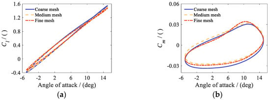
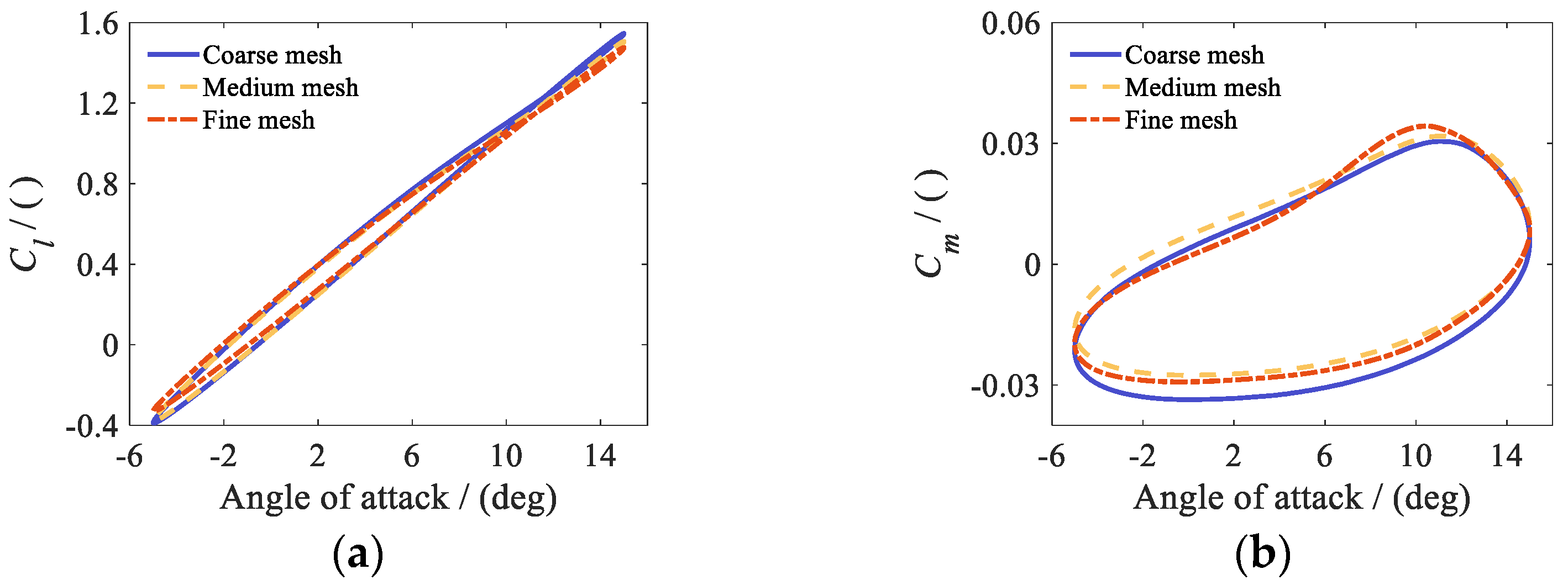
The mesh comparison used coarse, medium, and fine meshes of approximately 39,000, 55,000, and 91,000 cells, respectively. Figure 2a,b show that the medium and fine meshes give similar hysteresis loops and peak values for the lift and pitching moment coefficients. Relative to the fine mesh, the differences in Cl and Cm were 2.26% and 4.25% for the coarse mesh and 1.40% and 3.70% for the medium mesh. The relative differences are computed using the same range-normalized mean absolute error as in Equation (14).
Figure 2.
Comparison of CFD results for three mesh resolutions: (a) lift coefficient Cl; (b) pitching moment coefficient Cm.
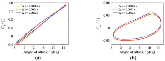
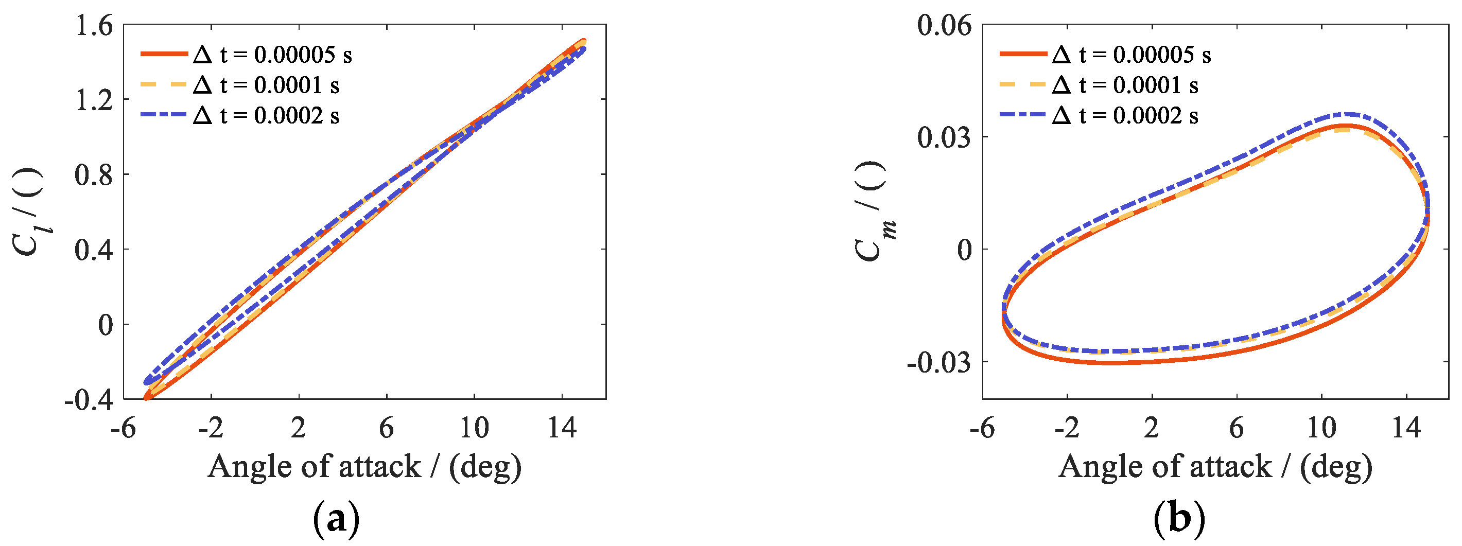
Figure 3.
Comparison of CFD results for three physical time steps: (a) lift coefficient Cl; (b) pitching moment coefficient Cm.
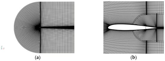
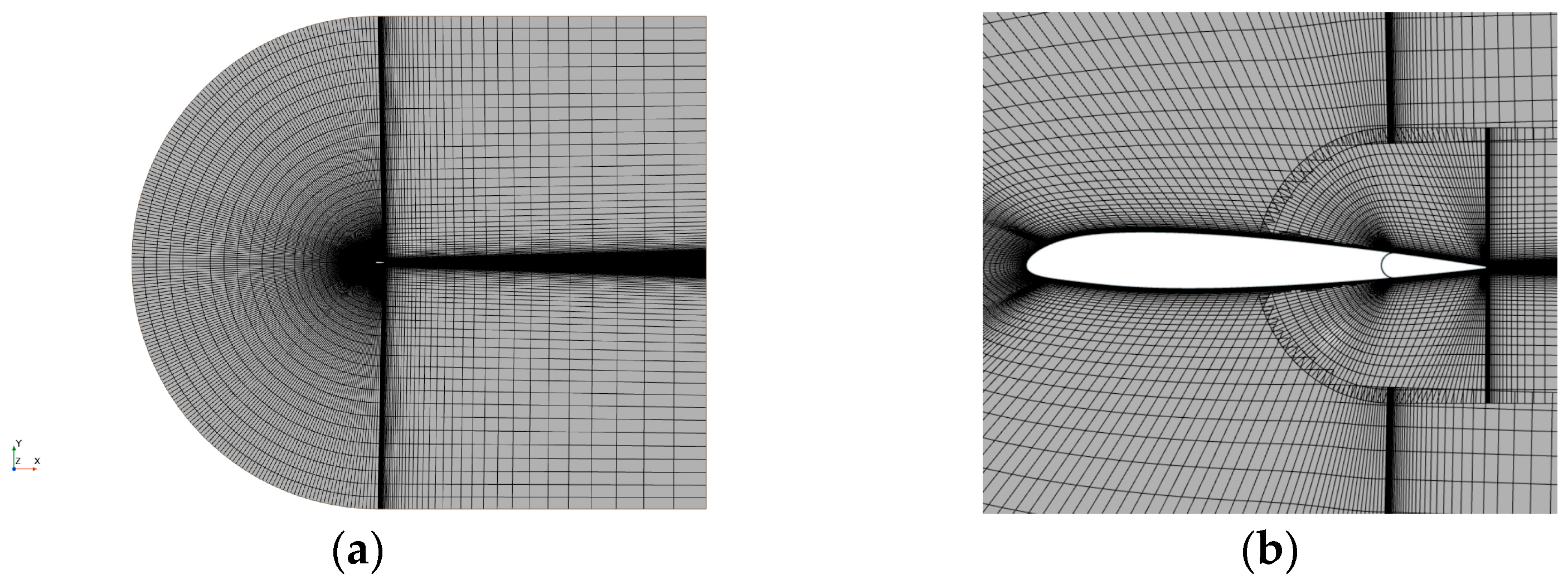
Figure 4.
Schematic of the overset mesh for the airfoil system: (a) far field; (b) airfoil and trailing-edge flap.
The time-step comparison on the medium mesh used 0.5 × 10⁻⁴, 1.0 × 10⁻⁴, and 2.0 × 10⁻⁴ s. As shown in Figure 3a,b, the two smaller steps gave similar coefficient histories and peak values. Relative to the smallest step, the differences in Cl and Cm were 2.15% and 4.86% for the largest step and 0.44% and 2.34% for the intermediate step. To balance accuracy and cost, subsequent simulations used the medium mesh and a physical time step of 1.0 × 10⁻⁴ s. For the case tested, the comparisons support the selected CFD settings, although the pitching moment coefficient was more sensitive than the lift coefficient to both mesh resolution and time-step size. Figure 4a,b show the far-field mesh and the mesh around the airfoil and trailing-edge flap.
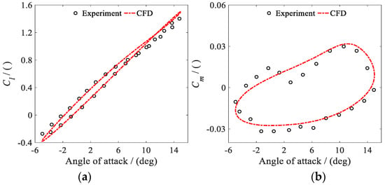
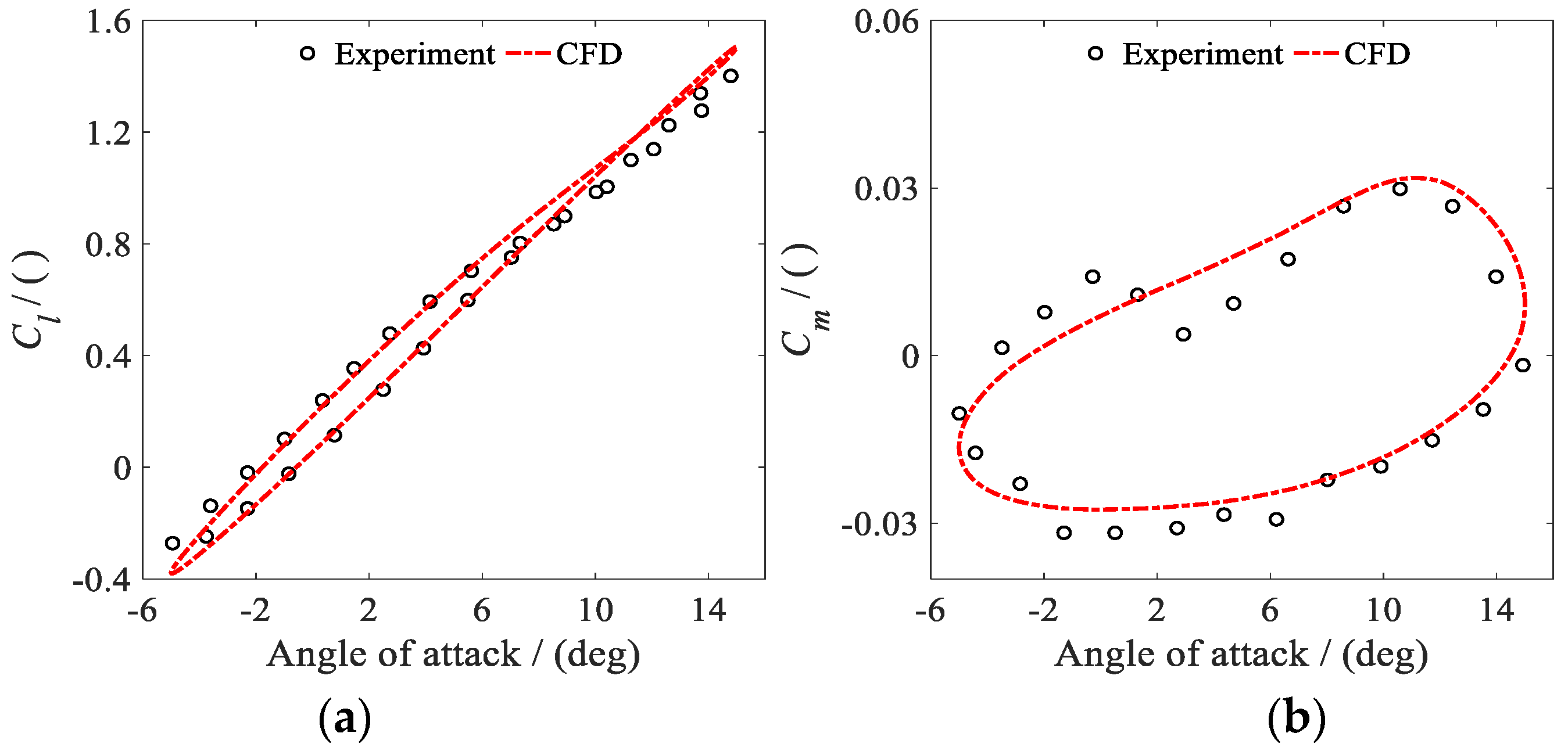
The airfoil geometry and experimental data in this section are both taken from Ref. [53]. The validation conditions are a pitch angle of α(t) = 5° + 10° × sin(ωt), a reduced frequency of k = 0.10, a Reynolds number of Re = 6.0 × 10⁵, and a Mach number of Ma = 0.09. The flap deflection angle is 0°. Figure 5a,b compare the CFD results with the experimental data for the airfoil under mild dynamic stall.
Figure 5.
Comparison of CFD results with experimental data: (a) lift coefficient Cl; (b) pitching moment coefficient Cm.
Figure 5a,b show that the CFD results agree well with the experimental data in Ref. [53]. The overall trends and hysteresis characteristics of Cl and Cm are generally consistent with the measurements. However, some deviations remain near the local peaks of Cm. These deviations may arise because Cm is more sensitive to the surface pressure distribution and the location of local flow separation. URANS also has some modeling error in resolving local unsteady separation during dynamic stall. Using the experimental data as the reference, the range-normalized mean absolute errors in Cl and Cm were 2.60% and 7.13%, respectively. Overall, the present CFD setup reasonably represents this mild dynamic-stall case.
CFD calculates the aerodynamic responses of the airfoil-flap system to prescribed motion inputs in each degree of freedom. The resulting input–output time series are used to train the ROMs. As the number of input dimensions increases, the curse of dimensionality makes it prohibitively expensive to generate the initial training samples by discrete-point sampling. This study uses Filtered White Gaussian Noise (FWGN) signals to excite the airfoil system. Independent FWGN signals are used for plunge, pitch, and the time-varying freestream. Flap deflection is generated using the low-frequency FWGN modulation coefficient method to satisfy practical actuation-frequency constraints. Input-signal parameters are given for each corresponding case in Section 4.
4. Validation and Results
This section validates the ROMs at three progressive levels: reconstruction of aerodynamic loads over the training interval, independent prediction and parameter extrapolation, and ROM blending over a wide Mach number range. The tests examine each ROM’s reconstruction performance, convergence characteristics, generalization, and extrapolation.
Section 4.1, Section 4.2 and Section 4.3 progressively increase the number of input degrees of freedom of the airfoil system. The inputs progress from pitch–flap and plunge–flap motions to coupled pitch–plunge–flap motion. They are then extended to complete-DOF inputs comprising plunge, pitch, flap deflection, and a time-varying freestream. The reconstruction capabilities of Standard DMDc and Hankel-DMDc are evaluated using the same CFD datasets. Section 4.1, Section 4.2 and Section 4.3 all use FWGN input signals of duration t = 3.0 s with a time step of Δt = 1.0 × 10⁻⁴ s. The FWGN sequences are generated by low-pass filtering Gaussian white noise and scaling the filtered signals to the target amplitudes for each degree of freedom. The randn function in MATLAB R2024a generates the white noise. To exclude the CFD startup transient, the interval t = 0.30–3.0 s is consistently used for identification and reconstruction. Section 4.4 fixes the model matrices and uses FWGN inputs excluded from training to test independent prediction, pitch-amplitude extrapolation, and long-horizon stability. Section 4.5 linearly blends local ROMs covering different Mach number intervals to assess prediction over a wide Mach number range. To quantify the overall deviation within each evaluation interval, this study uses the range-normalized mean absolute error [18], defined for each aerodynamic coefficient as follows:
where Ej denotes the relative error of aerodynamic coefficient j. The metric is used to evaluate reconstruction and independent-prediction errors for j = {Cl, Cd, Cm}. and y(ti) denote the ROM-calculated value and the CFD reference value, respectively, at discrete time ti. N denotes the number of samples in the evaluation interval.
The vibration-control algorithm limits the frequency components available for active trailing-edge flap deflection on a smart rotor. The actuation system cannot readily reproduce the continuous, high-frequency components in conventional FWGN signals. To strengthen selected low-order components, this study uses the low-frequency FWGN modulation coefficient method to generate the flap training input. The trailing-edge flap deflection signal is formed by superposing the Nf = 2–6 P harmonic components:
where n = {2, 3, 4, 5, 6} denotes the harmonic order. fn(t) denotes the random amplitude of the nth harmonic generated using low-frequency FWGN, with a range of 0.0–8.0° in this study. ϕn(t) denotes the random initial phase, ranging from 0.0° to 360.0°. Ω denotes the rotor angular speed, with 1P corresponding to 44.5 rad/s. Amplitude and phase modulation of the Nf = 2–6 harmonic components increases the excitation energy at the target frequencies while preserving input randomness. The frequency decomposition is further illustrated in Section 4.1. The low-frequency FWGN modulation coefficient method is also used to generate the flap excitation signals in all subsequent subsections.
4.1. Pitch–Flap and Plunge–Flap Motions
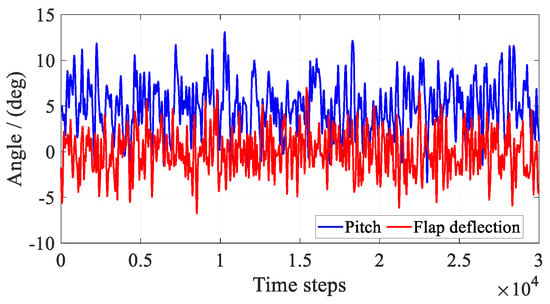
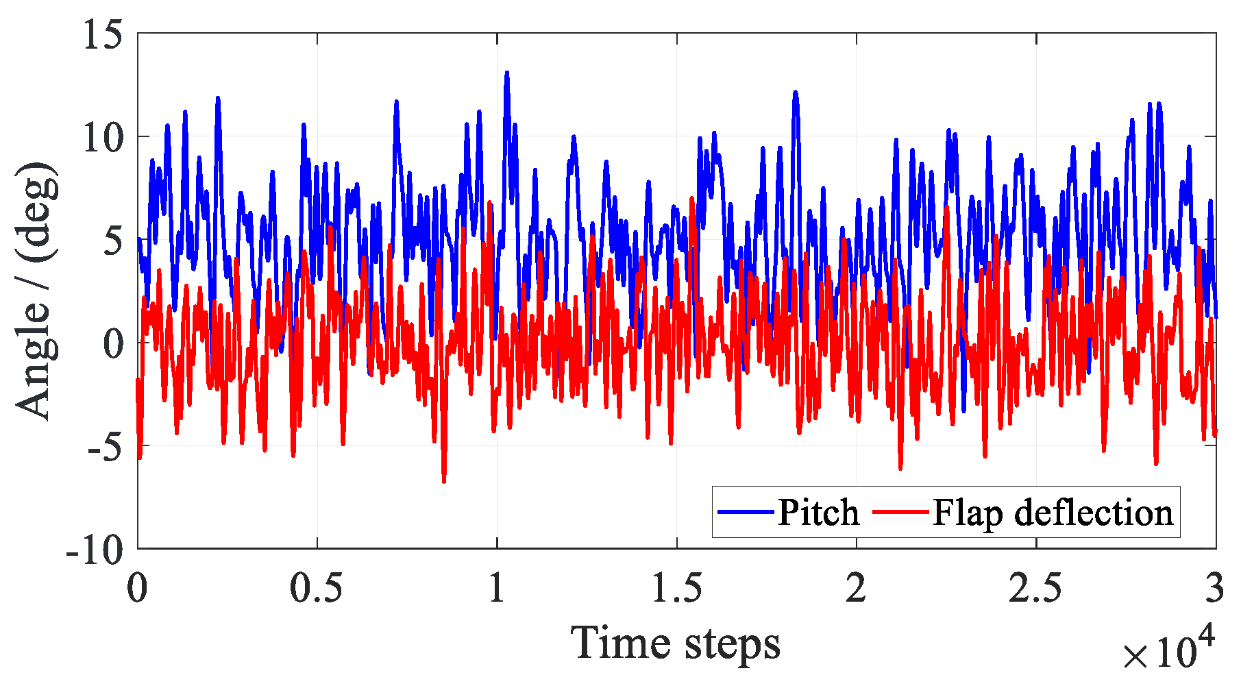
As the starting point of the progressive validation, this subsection examines pitch and plunge separately as the two primary motions of the main airfoil. Each motion is coupled with trailing-edge flap deflection to evaluate the reconstruction capabilities of the different DMDc models. The freestream Mach number is fixed at Ma = 0.30. Figure 6 first presents the FWGN excitation signals for the main-airfoil pitch and trailing-edge flap deflection. The instantaneous input vector uk for this case is expressed as:
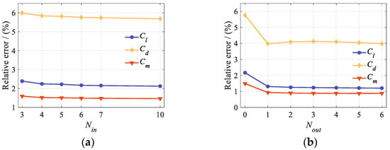
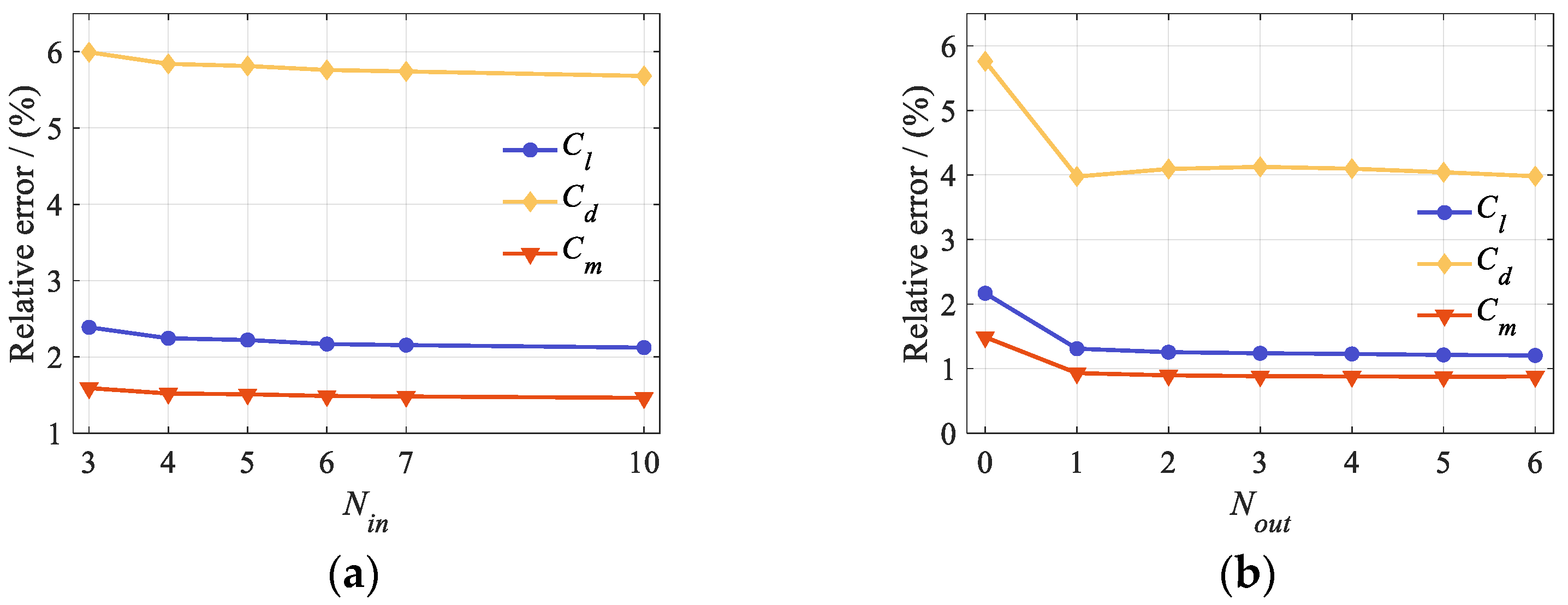
where αk denotes the pitch angle of the main airfoil, and βk denotes the flap deflection angle. Input delay and output delay embedding are introduced to represent memory effects. The pitch–flap inputs in Equation (16) and the corresponding CFD outputs were used to select the lag orders. Figure 7a shows Standard DMDc reconstruction errors versus Nin. For orders of 0, 1, and 2, the reconstructions diverged, and the state matrix had an eigenvalue with magnitude greater than one. These cases are omitted. Beyond order 6, errors decreased only slightly, while the model matrices grew. With Nin fixed at 6, Figure 7b shows Hankel-DMDc reconstruction errors versus Nout.
Figure 6.
Pitch and flap-deflection FWGN excitation signals.
Figure 7.
Reconstruction errors: (a) input lag order in Standard DMDc and (b) output-delay embedding order in Hankel-DMDc.
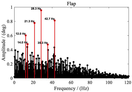
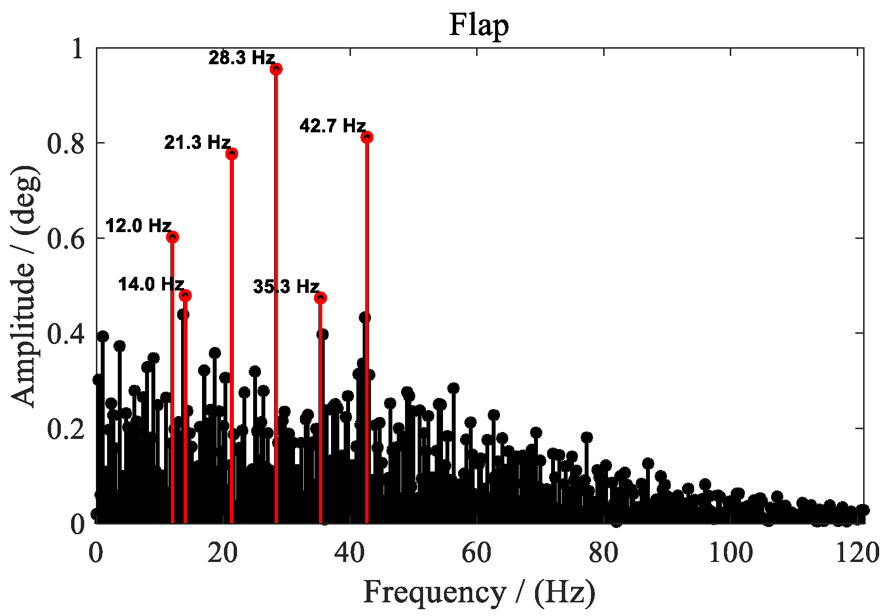
To balance reconstruction accuracy and model size, the reconstruction cases use six input lags for both models and three output delays for Hankel-DMDc. These hyperparameters remain unchanged in this and subsequent subsections. This study uses low-frequency FWGN modulation coefficients to increase the amplitudes of the target-frequency components in the flap input. Figure 8 presents the Fast Fourier Transform (FFT) results for the trailing-edge flap excitation. The amplitudes at the Nf = 2–6 harmonics are markedly increased.
Figure 8.
Flap-deflection frequency spectrum generated using the low-frequency FWGN modulation coefficient method.
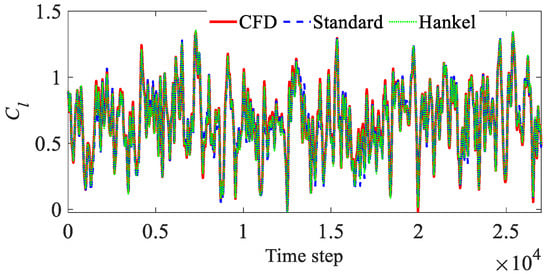
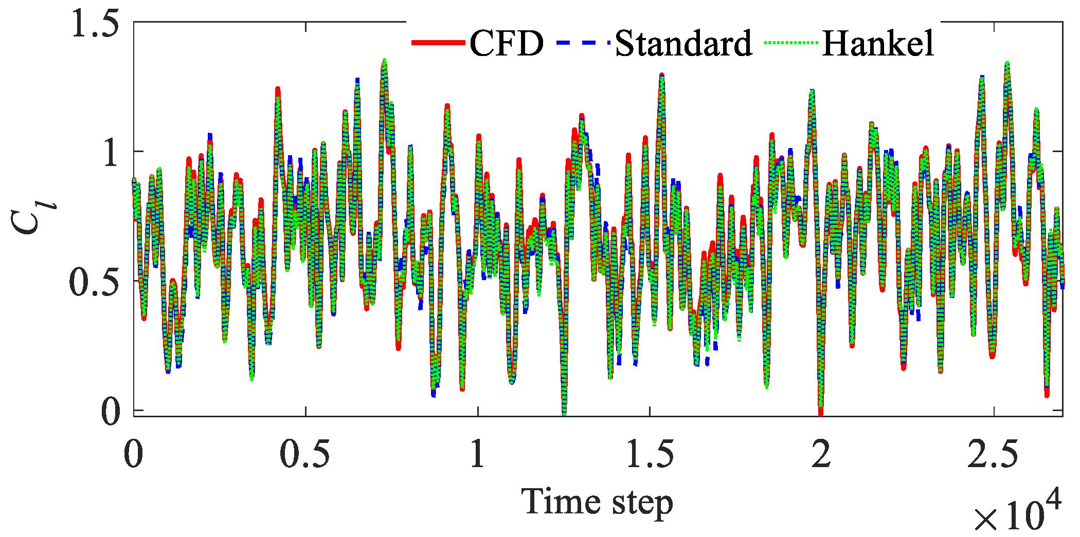
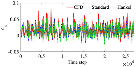
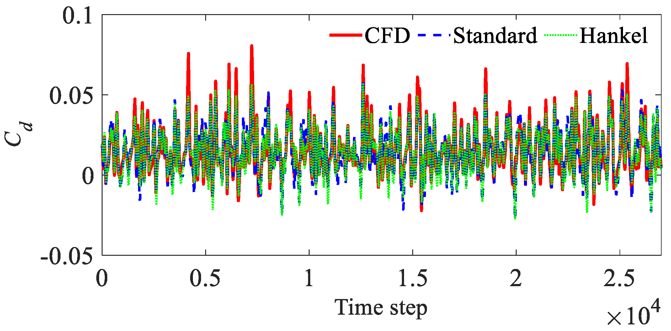
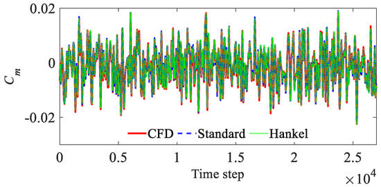
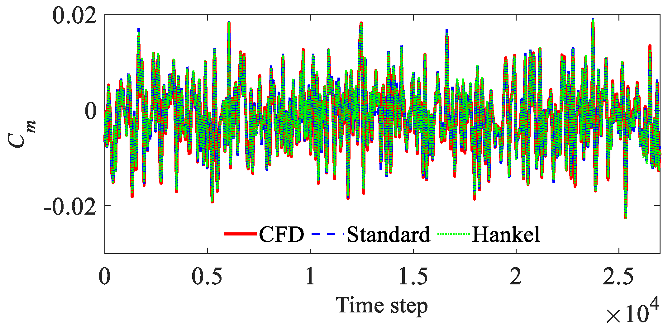
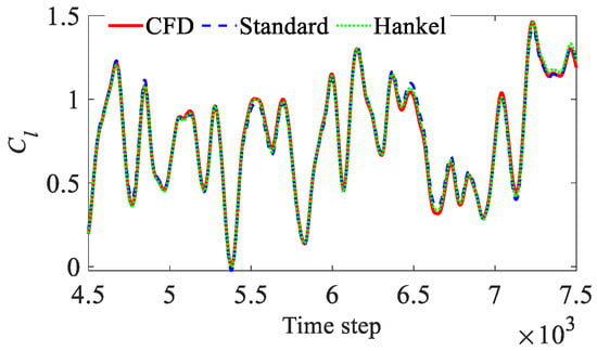
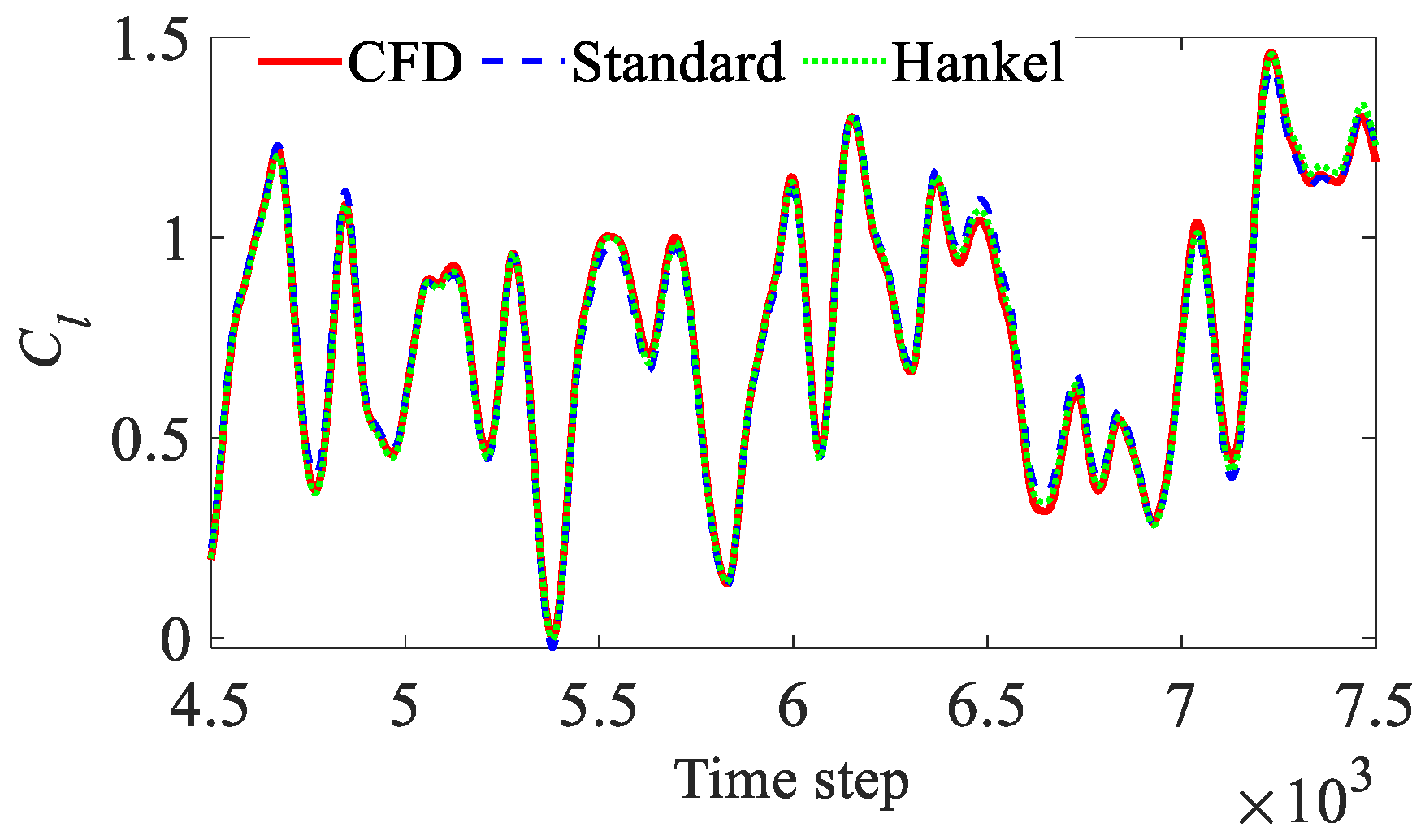
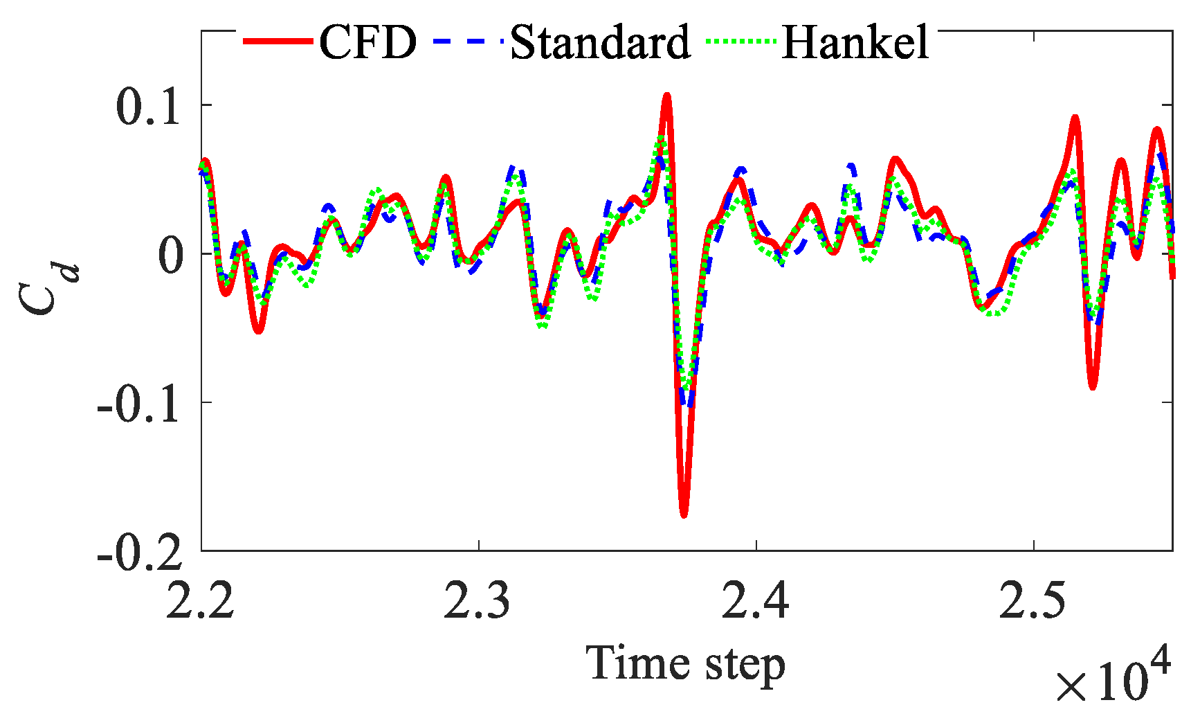
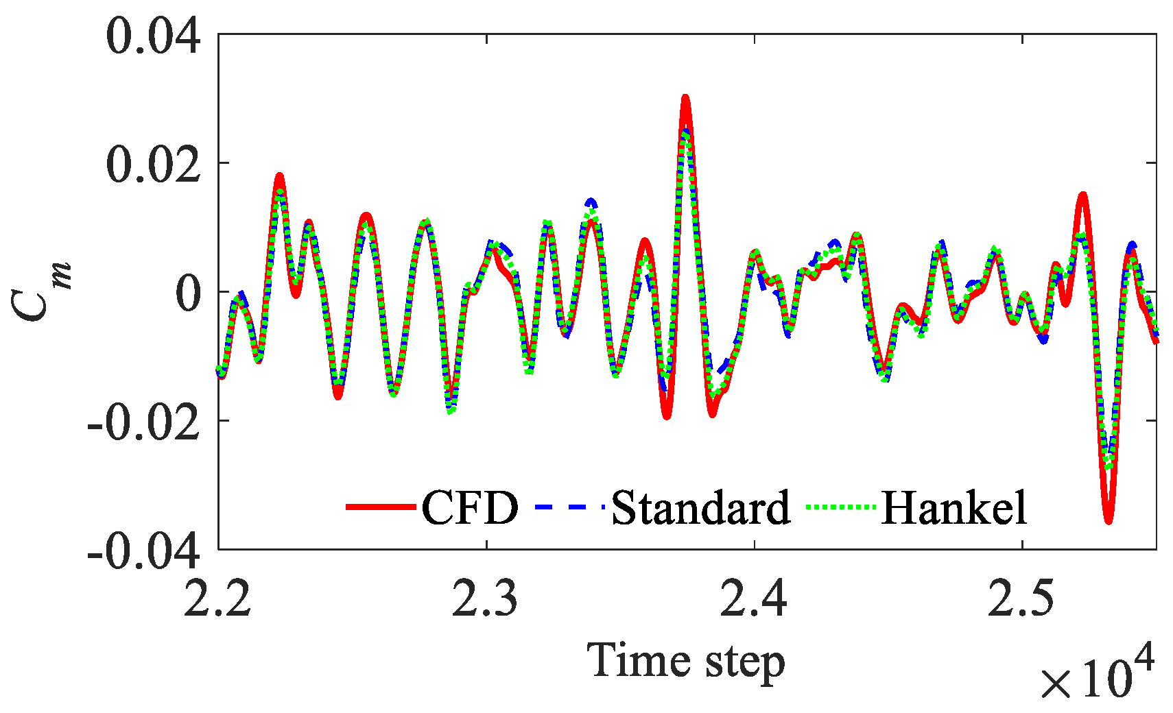
Figure 9, Figure 10 and Figure 11 present the training-interval reconstructions of Cl, Cd, and Cm obtained using Hankel-DMDc and Standard DMDc. Both methods reproduce the unsteady amplitude and phase variations of the aerodynamic coefficients. The reconstructed values also track the responses well in regions of rapid aerodynamic fluctuations. The Cl and Cm curves show good overall agreement. More pronounced local amplitude errors remain in Cd.
Figure 9.
CFD training data and ROM reconstructions of the lift coefficient Cl.
Figure 10.
CFD training data and ROM reconstructions of the drag coefficient Cd.
Figure 11.
CFD training data and ROM reconstructions of the pitching moment coefficient Cm.
Table 1 summarizes the reconstruction errors of the two DMDc methods over the full FWGN training-signal interval.
Table 1.
Reconstruction errors of aerodynamic coefficients.
Table 1 shows that Hankel-DMDc has lower overall errors than Standard DMDc for all three coefficients. This indicates that the output-delay state helps represent the system dynamics under broadband excitation.
Following the pitch–flap case, the plunge–flap input is examined. Like pitch, plunge is another dominant motion input governing the unsteady aerodynamic loads of an airfoil. The freestream remains at Ma = 0.30, and the main-airfoil pitch angle is held constant. The trailing-edge flap uses the same FWGN signal as in the preceding pitch–flap case. The instantaneous input vector uk is expressed as:
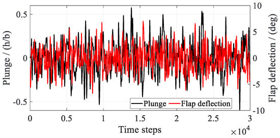
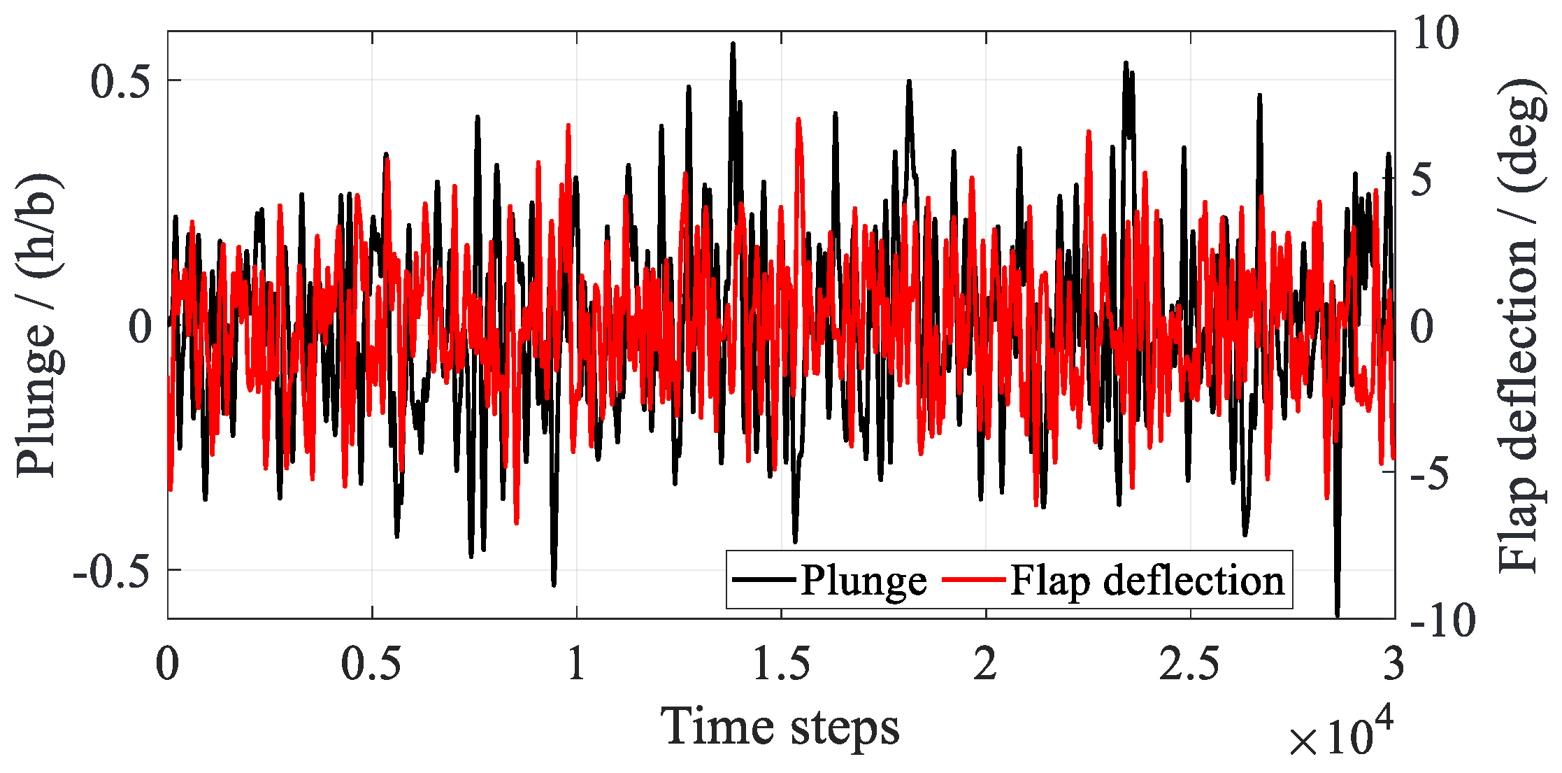
where denotes the dimensional plunge velocity at a discrete time. Figure 12 presents the FWGN excitation signals for plunge displacement and flap deflection used in the CFD simulation. The airfoil plunge motion is shown in nondimensional form, with b denoting the airfoil semi-chord. The signal segment t = 0.30–3.0 s is used for ROM training and reconstruction.
Figure 12.
FWGN excitation signals for plunge displacement and flap deflection.
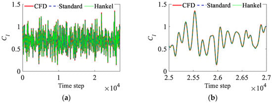
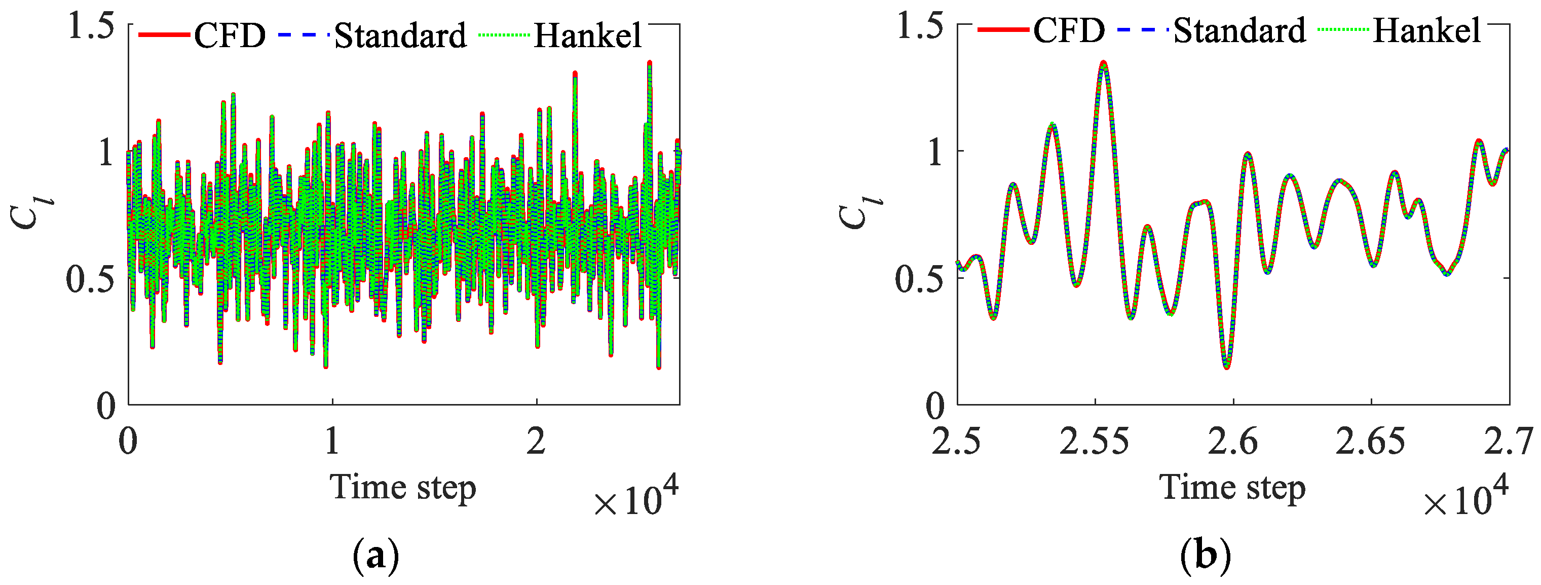
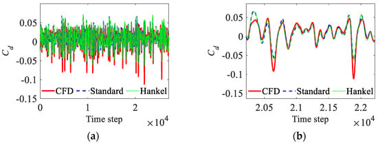
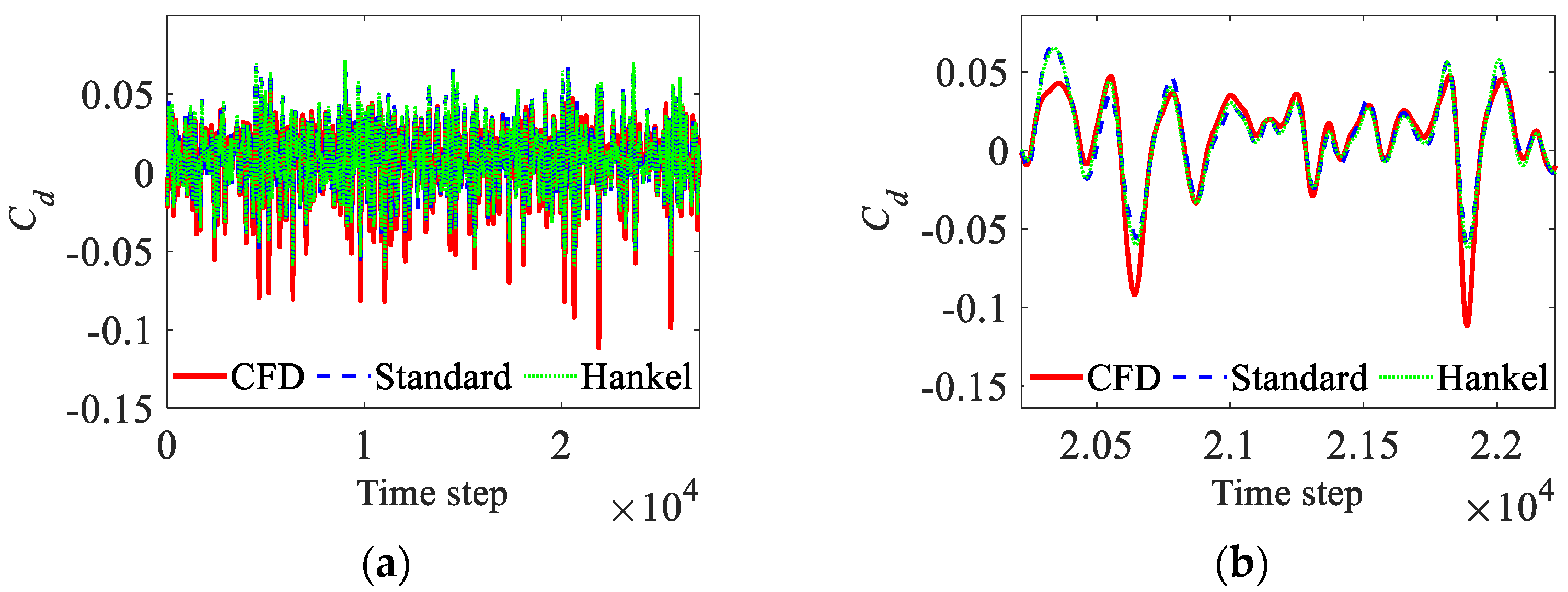
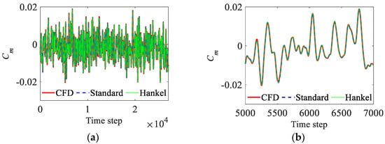
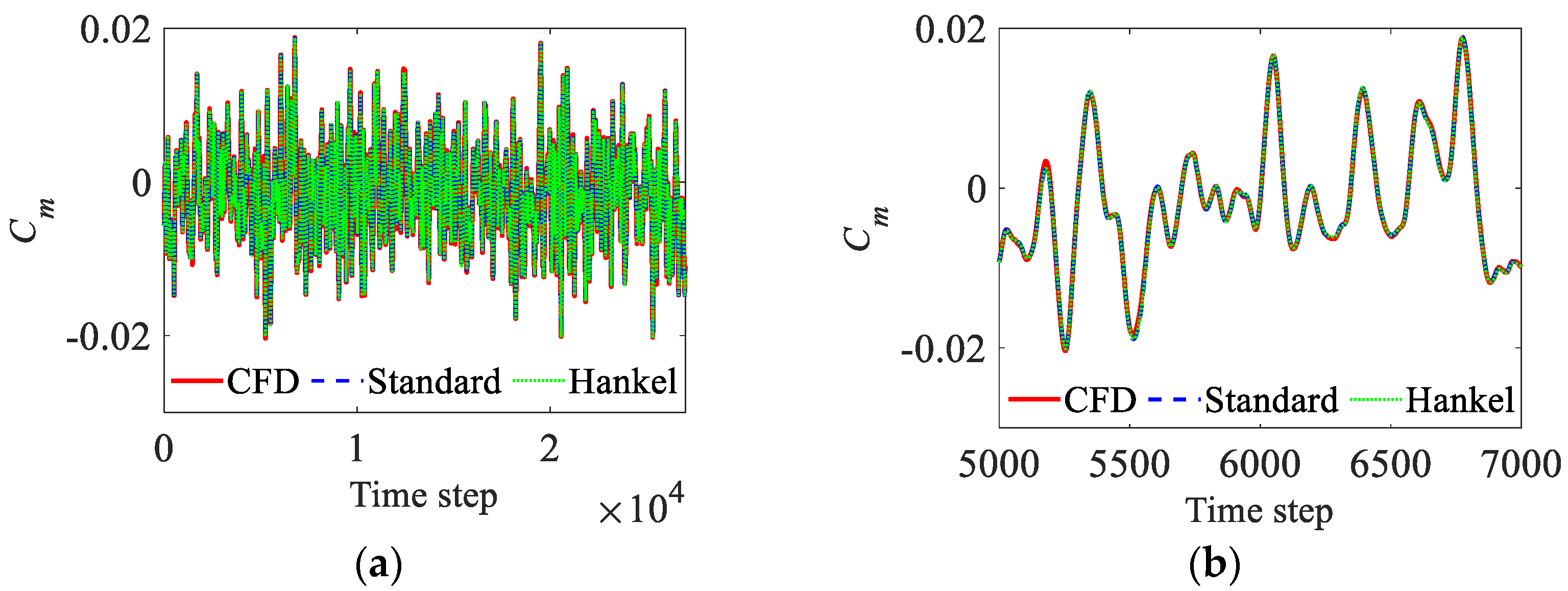
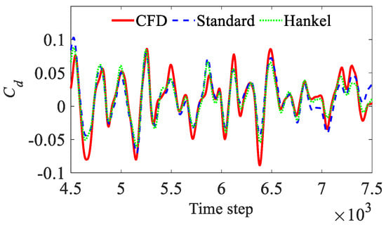
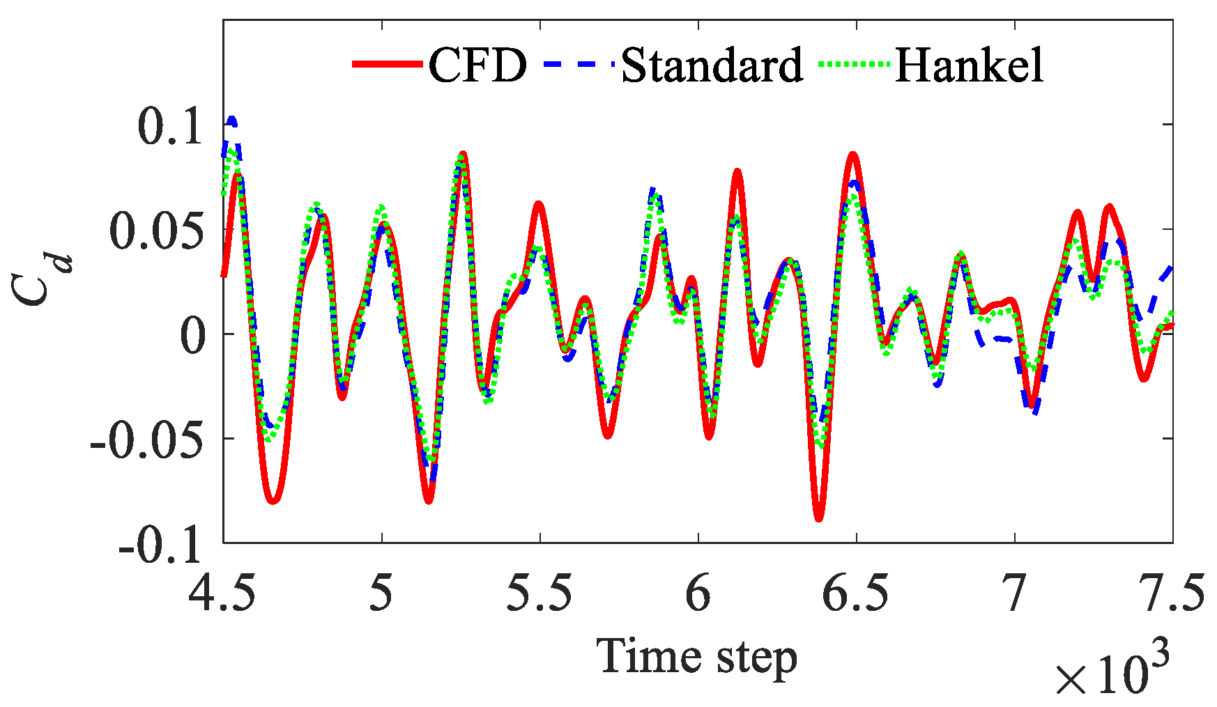
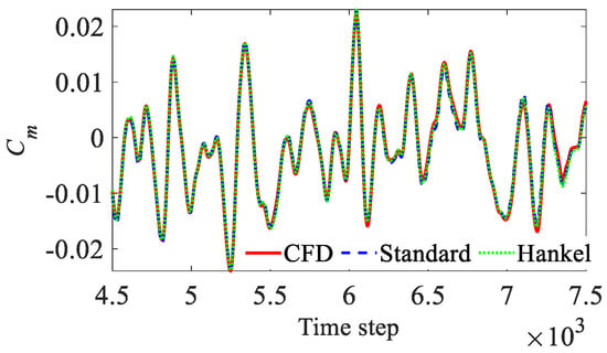
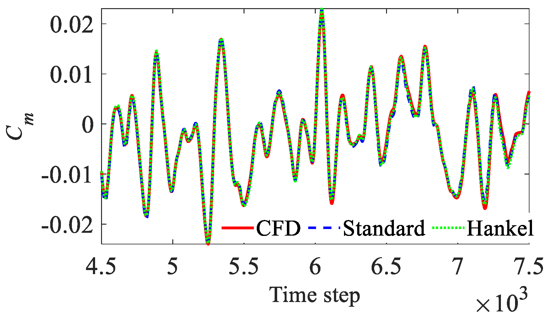
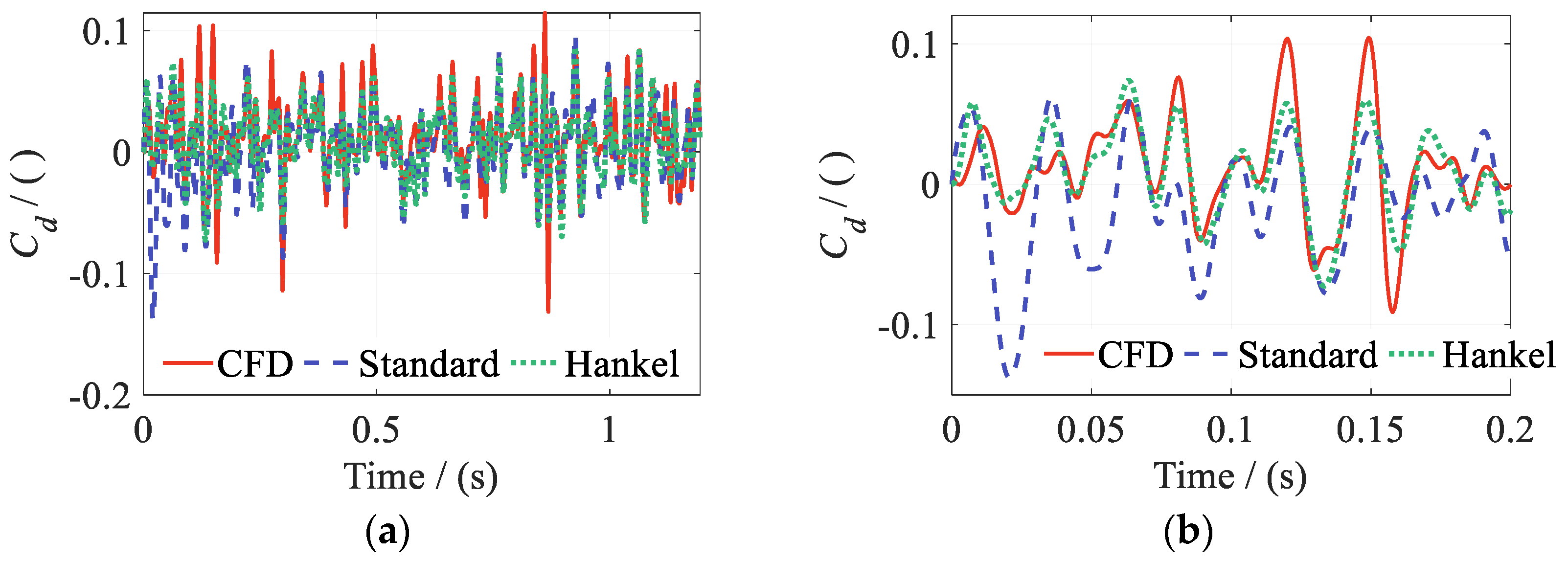
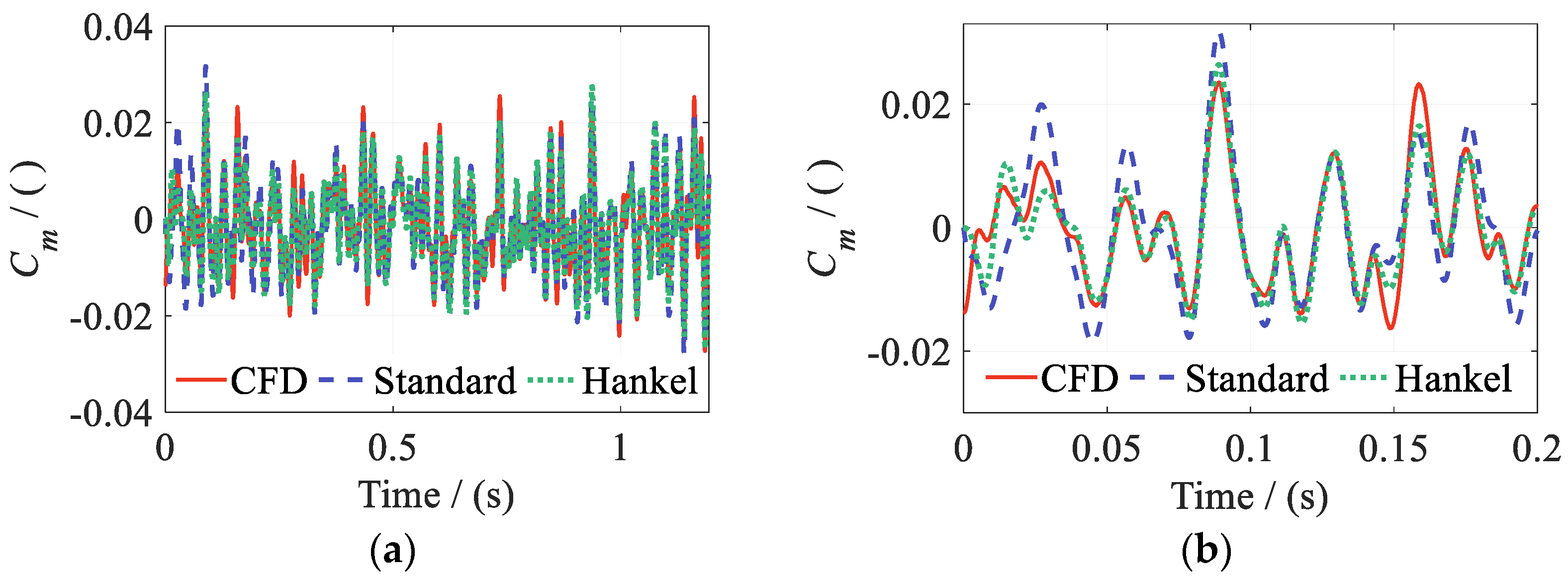
Figure 13, Figure 14 and Figure 15 compare the reconstructed Cl, Cd, and Cm from the two DMDc methods with the CFD results over the full interval. Close-up views of regions with rapid aerodynamic variations are also provided. Both methods reproduce the main amplitude and phase variations of Cl and Cm. Agreement with CFD is maintained even during rapid changes. Figure 14a,b show that the models capture the dominant variations in Cd, although amplitude deviations remain near some extrema.
Figure 13.
CFD training data and ROM reconstructions of Cl: (a) lift coefficient Cl; (b) detail of the signal.
Figure 14.
CFD training data and ROM reconstructions of Cd: (a) drag coefficient Cd; (b) detail of the signal.
Figure 15.
CFD training data and ROM reconstructions of Cm: (a) pitching moment coefficient Cm; (b) detail of the signal.
Table 2 summarizes the reconstruction errors of the aerodynamic coefficients over the full effective FWGN training interval. Table 2 shows that both Hankel-DMDc and Standard DMDc have low reconstruction errors for Cl and Cm. The errors for these two coefficients do not exceed 0.40%. Some reconstruction error remains in Cd. For this plunge–flap case, output delay embedding does not provide a clear improvement in reconstruction accuracy.
Table 2.
Reconstruction errors of aerodynamic coefficients.
Compared with the time-consuming CFD simulations, the ROMs are computationally efficient. Both DMDc methods complete model identification and reconstruction within a few seconds. Section 4.2 and Section 4.3 progressively increase the number of input degrees of freedom and introduce a time-varying freestream. This progressive validation further examines the reconstruction capabilities of the two DMDc methods.
4.2. Coupled Plunge-Pitch–Flap Motion
Building on the preceding cases with a single primary motion input, this subsection examines the reconstruction accuracy of the two DMDc methods under simultaneous plunge, pitch, and flap-deflection excitation. The effective angle of attack is influenced jointly by plunge and pitch. Coupling between these two inputs becomes more pronounced at larger motion amplitudes. The freestream Mach number remains fixed at Ma = 0.30. The instantaneous input vector uk is expressed as:
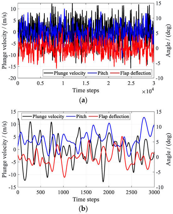
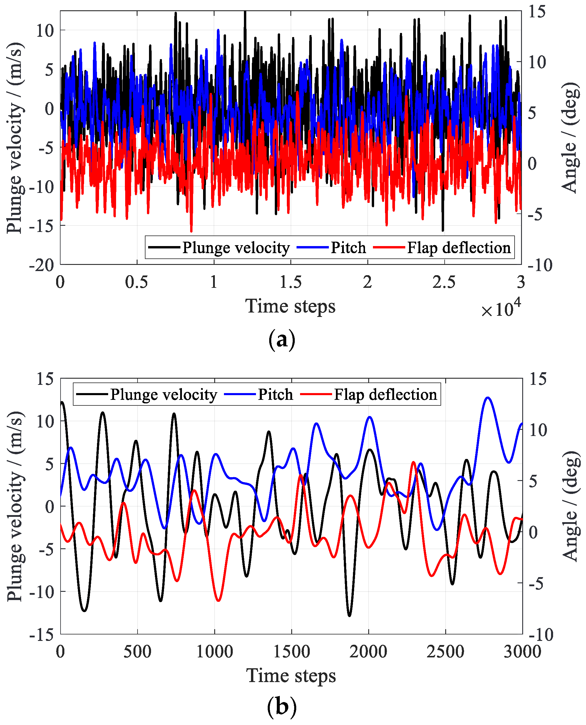
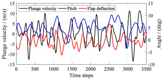
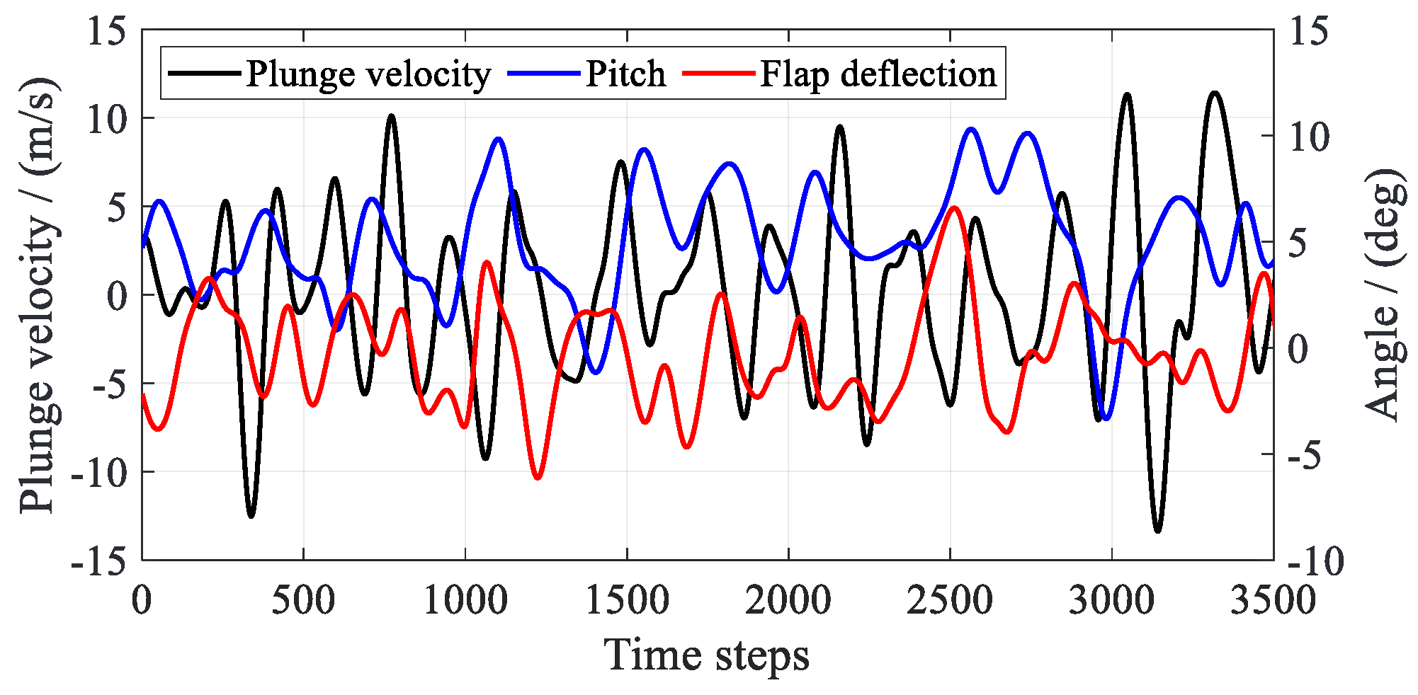
The FWGN input signal for each degree of freedom has a total duration of t = 3.0 s. The effective interval used for model identification is t = 0.30–3.0 s, as shown in Figure 16a. The segment t = 0.75–1.05 s is also presented in Figure 16b. This segment contains the strongest fluctuations across the input degrees of freedom.
Figure 16.
FWGN excitation signals for each degree of freedom: (a) full signal over t = 0.0–3.0 s; (b) selected signal segment.
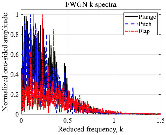
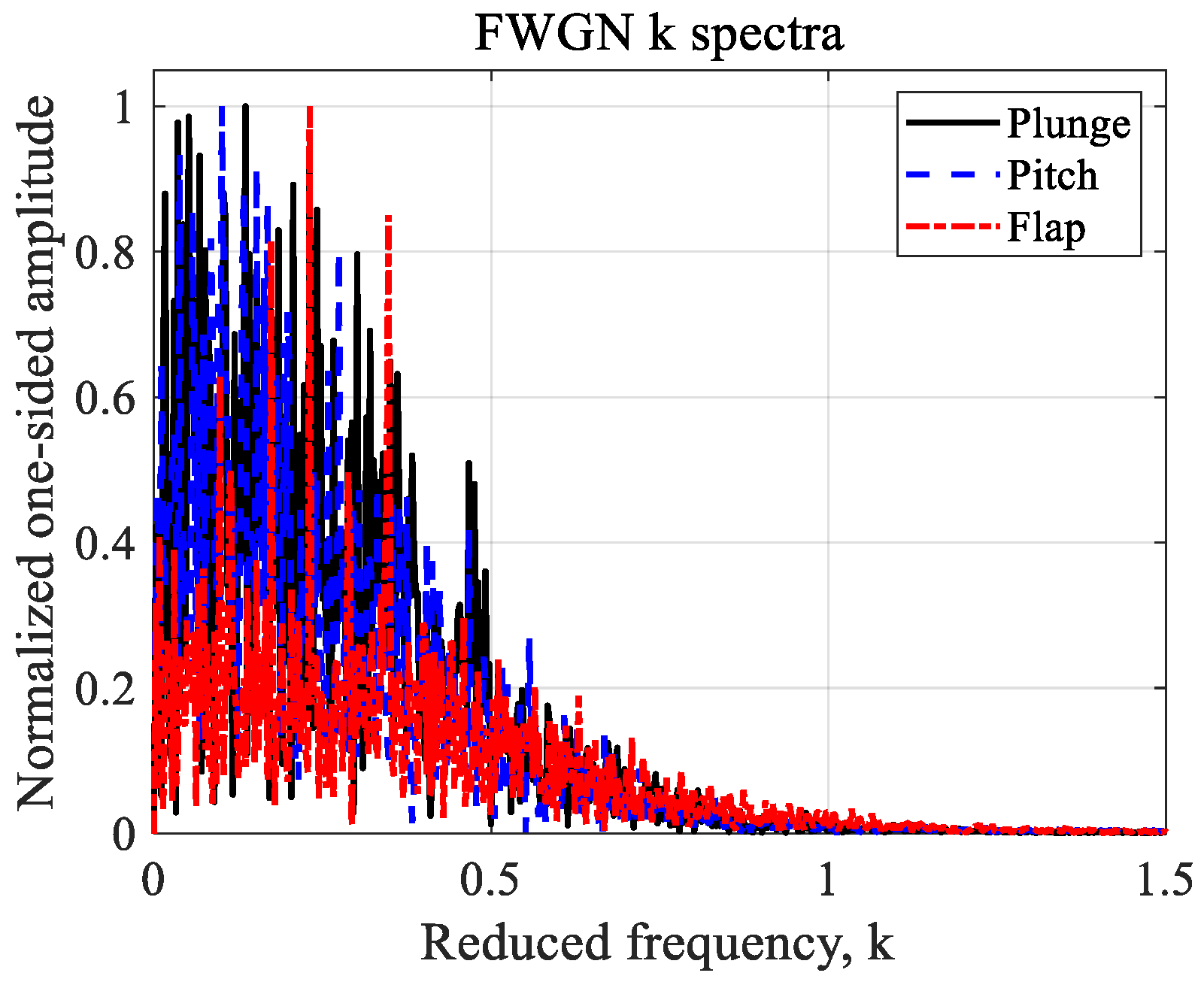
Figure 17 presents the FFT results and nondimensional reduced-frequency distributions of the full excitation signals for each degree of freedom. The FWGN bandwidth excites airfoil aerodynamic responses ranging from quasi-steady behavior through pronounced unsteady behavior to higher-frequency unsteady behavior.
Figure 17.
FFT results and reduced-frequency distributions of the FWGN signals.
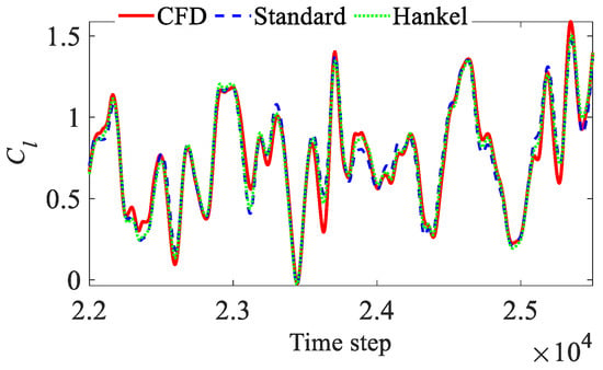
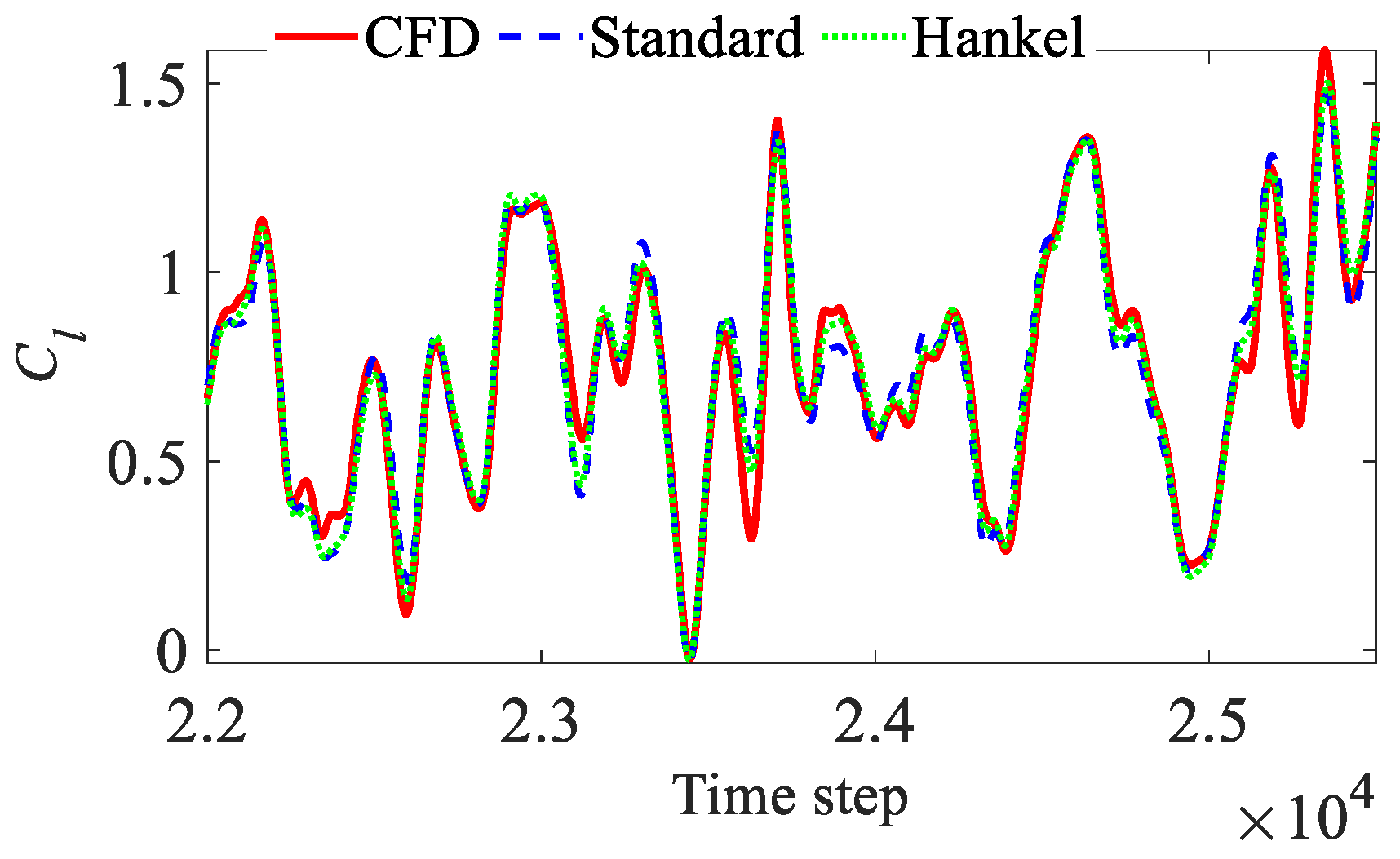
Figure 18, Figure 19 and Figure 20 show Cl, Cd, and Cm for the inputs in Figure 16a,b, with further amplitude and phase details. Both DMDc methods capture the main trends. Cl and Cm agree well with CFD and are important for rotor aeroelastic analysis. Both methods accurately reconstruct the phase of Cd, but amplitude deviations remain at local peaks. Reconstruction errors over the full effective training interval are summarized below.
Figure 18.
CFD data and ROM reconstructions of Cl.
Figure 19.
CFD data and ROM reconstructions of Cd.
Figure 20.
CFD data and ROM reconstructions of Cm.
Table 3 shows that Hankel-DMDc achieves higher identification accuracy for the key aerodynamic components Cl and Cm. Standard DMDc has a larger reconstruction error for Cd. The effective angle of attack is determined jointly by plunge and pitch. For the coupled plunge–pitch–flap case examined here, output delay embedding helps improve aerodynamic reconstruction accuracy. Comparing Table 1, Table 2 and Table 3 shows that the reconstruction errors of both methods generally remain of a similar order of magnitude as the number of motion-input degrees of freedom increases. The errors do not increase monotonically.
Table 3.
Reconstruction errors of aerodynamic coefficients.
4.3. Coupled Motion with Time-Varying Freestream
Building on Section 4.1 and Section 4.2, this subsection introduces a time-varying freestream Mach number. Complete-DOF inputs comprising plunge, pitch, flap deflection, and a time-varying freestream are constructed. The ability of the DMDc models to represent coupling among multiple inputs is then evaluated.
The rapid rotation and lead–lag motion of helicopter rotor blades cause the freestream velocity at an airfoil section to vary substantially within a cycle. This subsection uses airfoil lead–lag motion to simulate the time-varying freestream. Under these conditions, the wake leaves the trailing edge at a nonuniform velocity. The airfoil motion inputs and time-varying freestream are coupled. The instantaneous complete-DOF input vector uk is defined as:
where Ma(t) denotes the time-varying freestream Mach number. These four input degrees of freedom jointly drive the unsteady aerodynamic response. The FWGN motion-excitation signals are the same as those in Section 4.2. A time-varying freestream is added and expressed as:
where Ma0 denotes the mean Mach number, Ma_Amp denotes the amplitude of the Mach number fluctuation, and fMa denotes the freestream variation frequency. Using the BO105 rotor parameters as a reference, the freestream at the blade section r = 0.5R corresponds to approximately MΩ0.5 = 0.30. Ma_Amp is set to 0.10. The velocity fluctuation can be expressed through an equivalent advance ratio at r = 0.5R:
where V denotes the freestream velocity, and Ω denotes the rotor angular speed. This velocity fluctuation covers a broad range of local rotor freestream variations. The freestream variation frequency is set to fMa = 7.0 Hz. The Mach number therefore varies within Ma = 0.20–0.40. The dynamic characteristics of the governing flow equations change with the Mach number.
Figure 21 presents the t = 2.50–2.85 s of the FWGN signals for each degree of freedom. The aerodynamic coefficients exhibit their strongest fluctuations within this segment.
Figure 21.
Selected segment of the FWGN training inputs for each degree of freedom.
Figure 22, Figure 23 and Figure 24 compare the identification and reconstruction results of Hankel-DMDc and Standard DMDc for Cl, Cd, and Cm over the selected interval. Both methods reproduce the main trends even during strong aerodynamic fluctuations. The phases of the reconstructed responses agree well with CFD. These results indicate that both methods capture the coupled responses of a multiple-input/multiple-output system with pronounced unsteady effects. Both methods show good overall reconstruction accuracy. Table 4 summarizes the errors over the full interval t = 0.30–3.0 s.
Figure 22.
Training and reconstructed lift coefficient Cl.
Figure 23.
Training and reconstructed drag coefficient Cd.
Figure 24.
Training and reconstructed pitching moment coefficient Cm.
Table 4.
Reconstruction errors of aerodynamic coefficients.
Table 4 shows that Hankel-DMDc has lower reconstruction errors than Standard DMDc for all three coefficients. Introducing delayed states thus generally improves the identification of an unsteady system with memory effects and strong coupling. Comparing Table 3 and Table 4 shows that adding the time-varying freestream strengthens the unsteady aerodynamic behavior. The reconstruction errors of both methods consequently increase. Hankel-DMDc nevertheless has lower overall reconstruction errors than Standard DMDc.
Section 4.1, Section 4.2 and Section 4.3 complete a progressive reconstruction validation from single and coupled motion inputs to complete-DOF inputs. This provides the basis for testing ROM generalization and extrapolation using inputs excluded from training in Section 4.4 and Section 4.5.
4.4. Prediction and Pitch-Amplitude Extrapolation
Section 4.1, Section 4.2 and Section 4.3 validated the reconstruction capabilities of the two DMDc models for unsteady aerodynamics by progressively increasing the number of input degrees of freedom. This subsection evaluates the independent prediction performance, convergence characteristics, and generalization of Standard DMDc and Hankel-DMDc using FWGN inputs not used in training and the corresponding CFD results. Extrapolation is further evaluated by scaling only the pitch amplitude.
All ROM predictions are initialized using y(0) = 0 ∈ ℝ3. The models then recursively predict the airfoil coefficients Cl, Cd, and Cm.
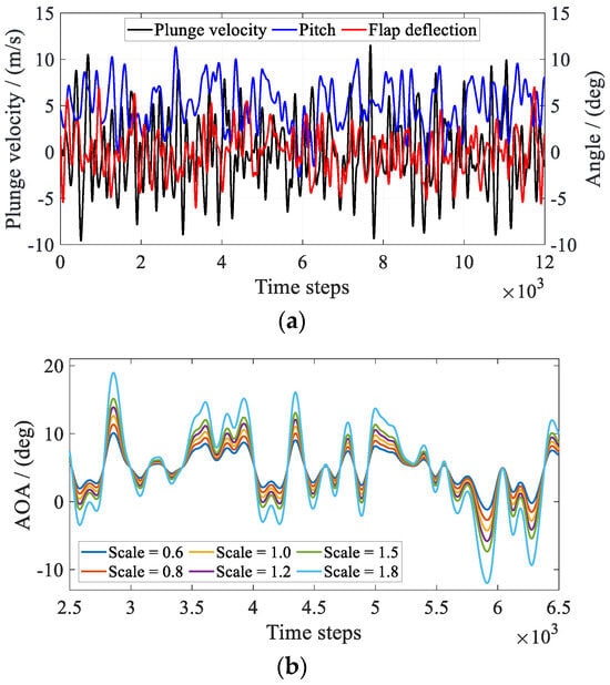
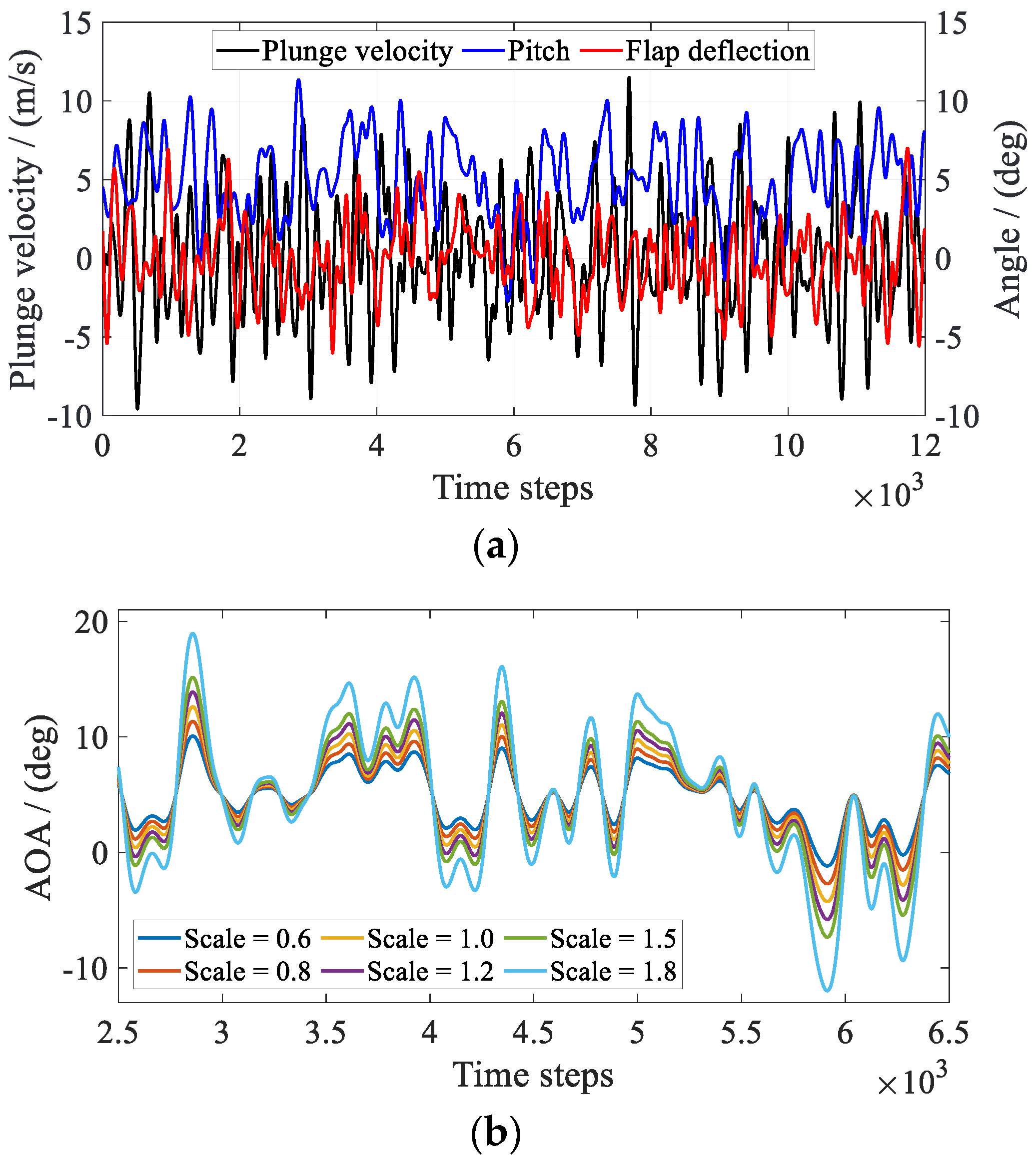
In rotor flight, airfoil pitch and plunge inputs contain multiple harmonic components. This subsection therefore uses FWGN signals containing multiple harmonics to validate prediction performance. Complex freestream conditions can also cause large, abrupt changes and fluctuations in the angle of attack. To test generalization and extrapolation with respect to pitch, one FWGN signal is used as the baseline. Multiple prediction-input signals are obtained by scaling its pitch component. Pitch-amplitude extrapolation is defined by scaling the generated FWGN amplitude while keeping its mean unchanged:
where λα denotes the pitch-amplitude scaling factor, with λα = {0.6, 0.8, 1.0, 1.2, 1.5, 1.8}. Each excitation signal has a duration of 2.0 s. αFWGN(t) denotes the airfoil pitch input. The scaled FWGN signal retains and changes only the fluctuations of αFWGN(t). The plunge, flap-deflection, and time-varying freestream amplitudes remain unchanged and are consistent with Section 4.3. Changes in error therefore arise only from changes in the pitch amplitude, providing a single-factor pitch-amplitude extrapolation test.
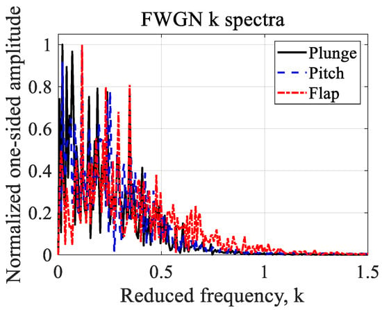
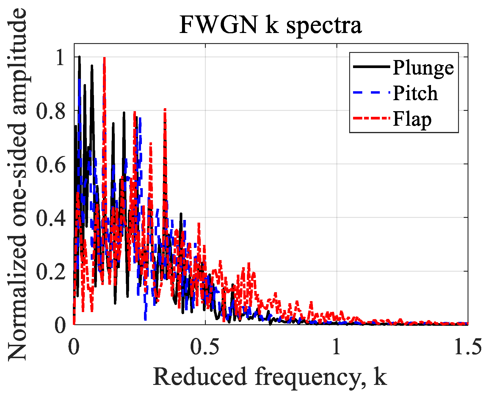
To exclude the CFD startup transient, ROM outputs over t = 0.80–2.0 s are compared with CFD. The baseline FWGN signals are shown in Figure 25a. The pitch signals for different scaling factors λα are shown in Figure 25b. The reduced frequencies of the baseline FWGN signal with λα = 1.0 are shown in Figure 26. This independent-prediction input covers the main frequency band, including low frequencies and frequencies at which unsteady effects are pronounced.
Figure 25.
FWGN signals for each degree of freedom: (a) baseline complete-DOF FWGN signals (λα = 1.0); (b) details of the scaled pitch inputs.
Figure 26.
Reduced frequencies of the baseline FWGN prediction-input signal (λα = 1.0).
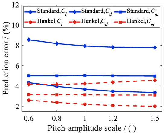
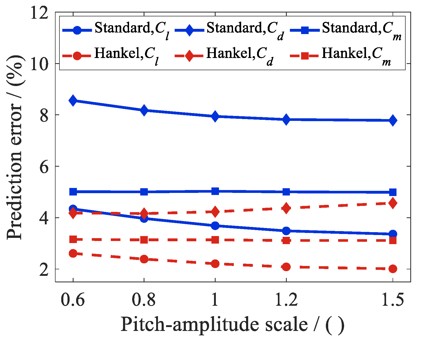
This subsection evaluates prediction accuracy and numerical stability separately. Accuracy is quantified by the deviation from the CFD reference using Equation (14). Numerical stability is assessed by whether disturbances grow persistently or the predicted response diverges during rolling prediction. Figure 27 presents the prediction errors of Standard DMDc and Hankel-DMDc for different pitch-amplitude scaling factors λα. Within λα = 0.6–1.5, the errors of both models do not increase substantially with the scaling factor. Standard DMDc has larger prediction errors for Cd, ranging from 7.79% to 8.56%. Hankel-DMDc maintains lower errors for all cases in Figure 27. Its augmented state constructed using delay coordinates explicitly retains historical information. This makes it better suited to representing unsteady memory effects under broadband excitation with a wide amplitude range.
Figure 27.
Prediction errors for different pitch-amplitude scaling factors.
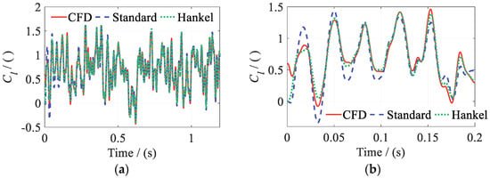
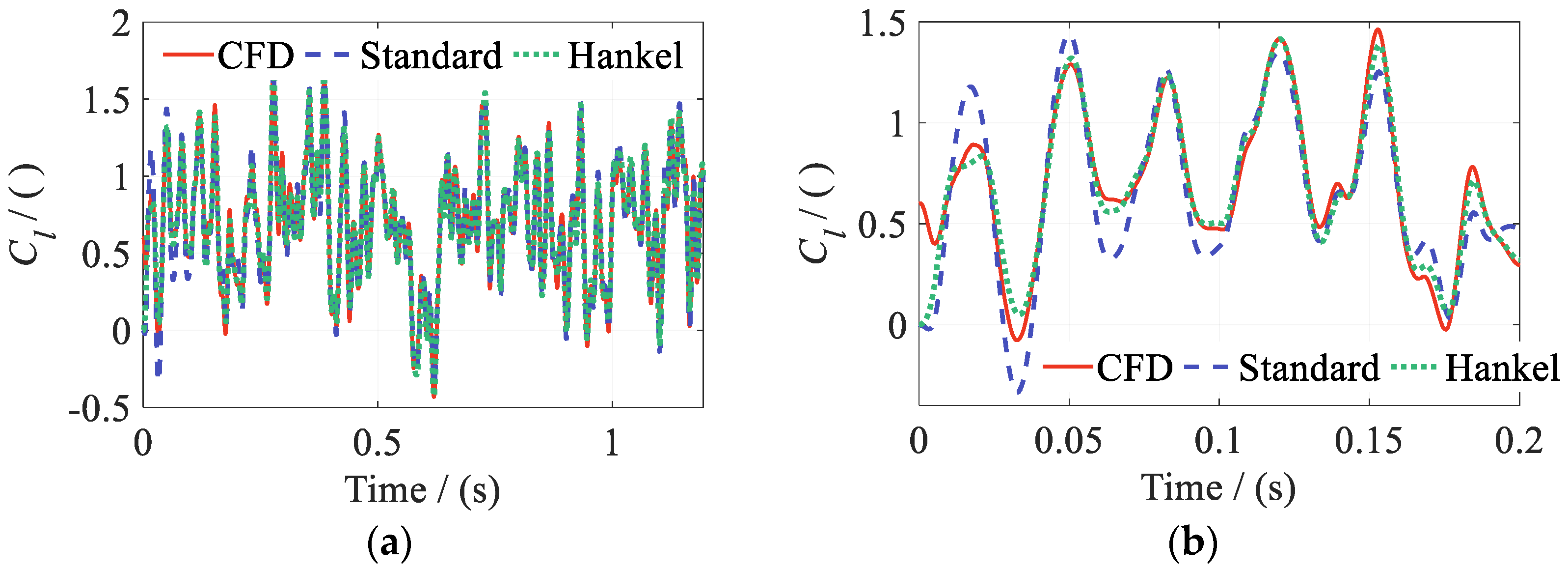
The predictions for a pitch FWGN amplitude scaling factor of λα = 1.5 are presented in Figure 28, Figure 29 and Figure 30.
Figure 28.
Lift coefficient Cl for a pitch-amplitude scaling factor of λα = 1.5: (a) full signal; (b) initial convergence interval.
Figure 29.
Drag coefficient Cd for a pitch-amplitude scaling factor of λα = 1.5: (a) full signal; (b) initial convergence interval.
Figure 30.
Pitching moment coefficient Cm for a pitch-amplitude scaling factor of λα = 1.5: (a) full signal; (b) initial convergence interval.
Figure 28, Figure 29 and Figure 30 show that both models predict the main amplitude and phase characteristics of the aerodynamic coefficients well over the full prediction interval. Hankel-DMDc agrees more closely with CFD. Both models have amplitude errors in their predictions of Cd.
Unlike SBRF, which relies on output feedback, the present ROMs are initialized with y(0) = 0 ∈ ℝ3. The perturbation associated with y(0) decays rapidly. Figure 28b, Figure 29b and Figure 30b show that the ROM-predicted values converge quickly. No error accumulation or numerical divergence is observed over the long-horizon interval of t = 1.2 s, with Δt = 1.0 × 10⁻⁴ s. This behavior is particularly important for tight coupling between ROMs and rotor CSD models. Such coupled systems typically require many time steps to reach a converged solution. The observed behavior is consistent with the dynamics indicated by the model eigenvalues. Hankel-DMDc has a shorter initial convergence interval and smaller prediction errors than Standard DMDc.
The case with λα = 1.8 was evaluated separately from the prediction-error comparison in Figure 27 to probe the limits of pitch-amplitude extrapolation. The test examined whether the ROMs’ rolling predictions beyond the training range diverged, showed abrupt jumps, or exhibited clearly nonphysical outputs.
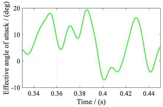
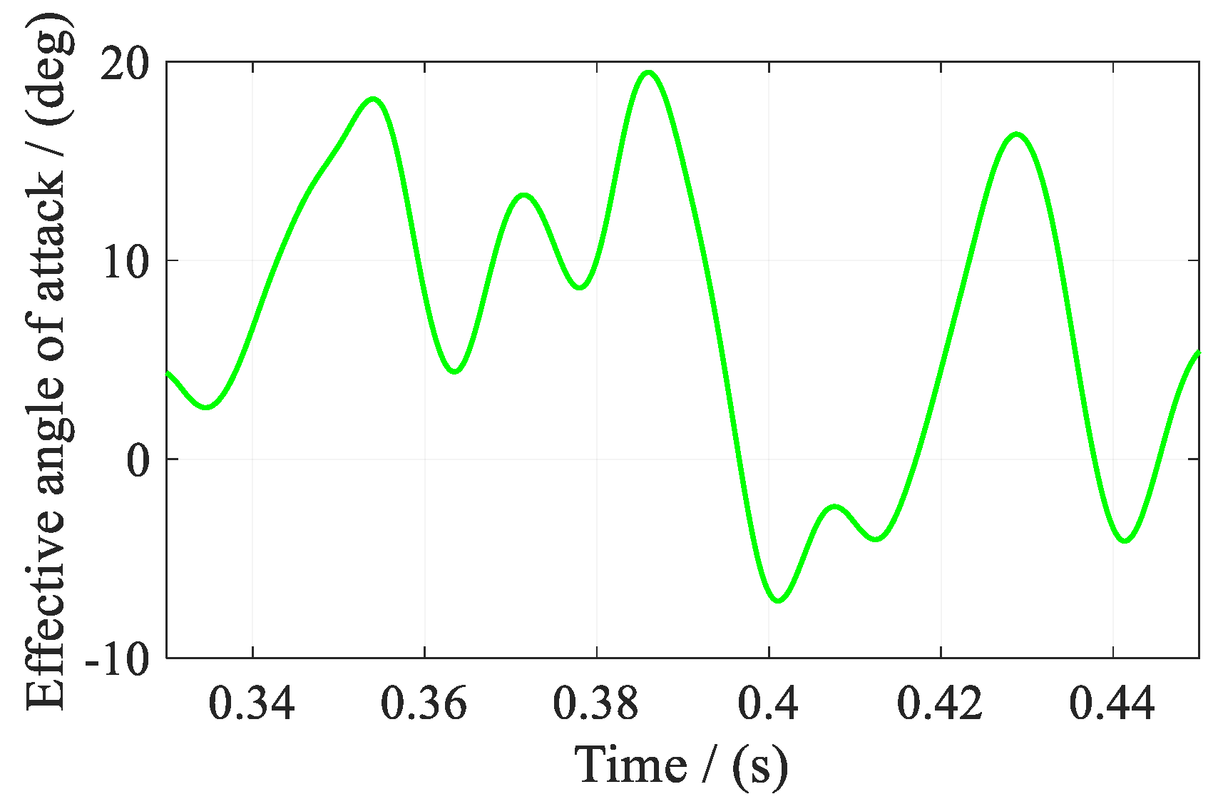
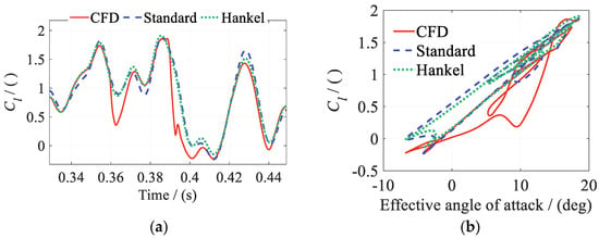
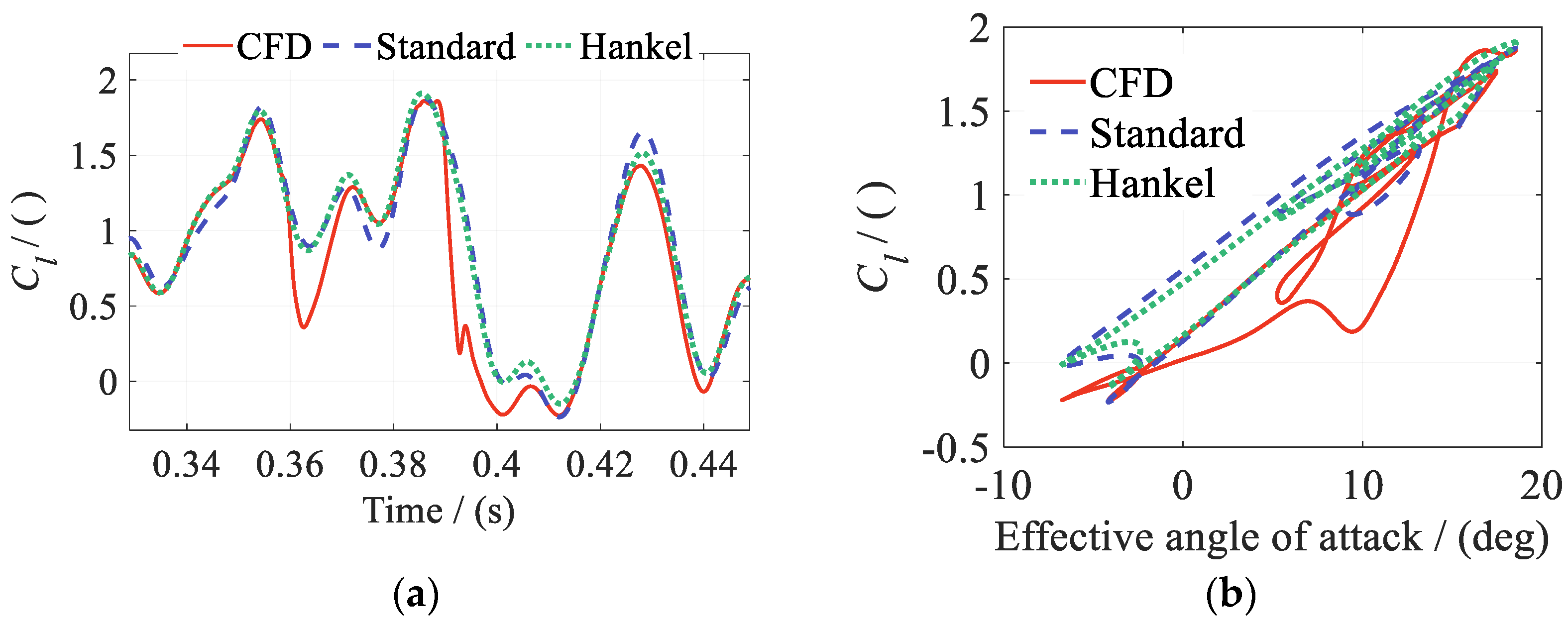
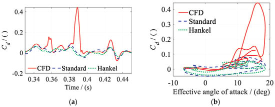
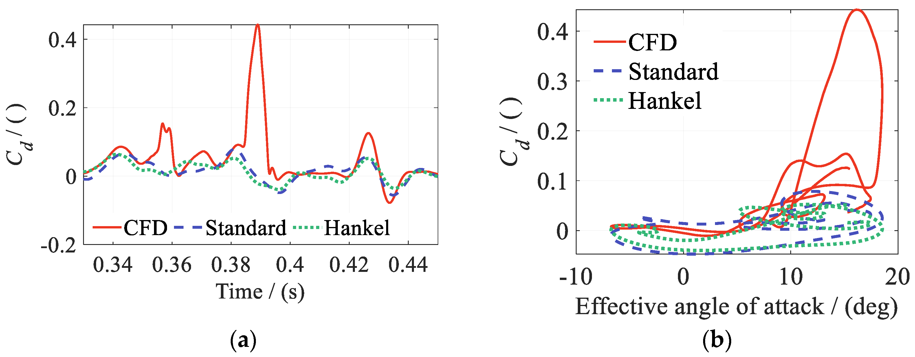
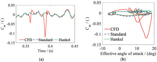
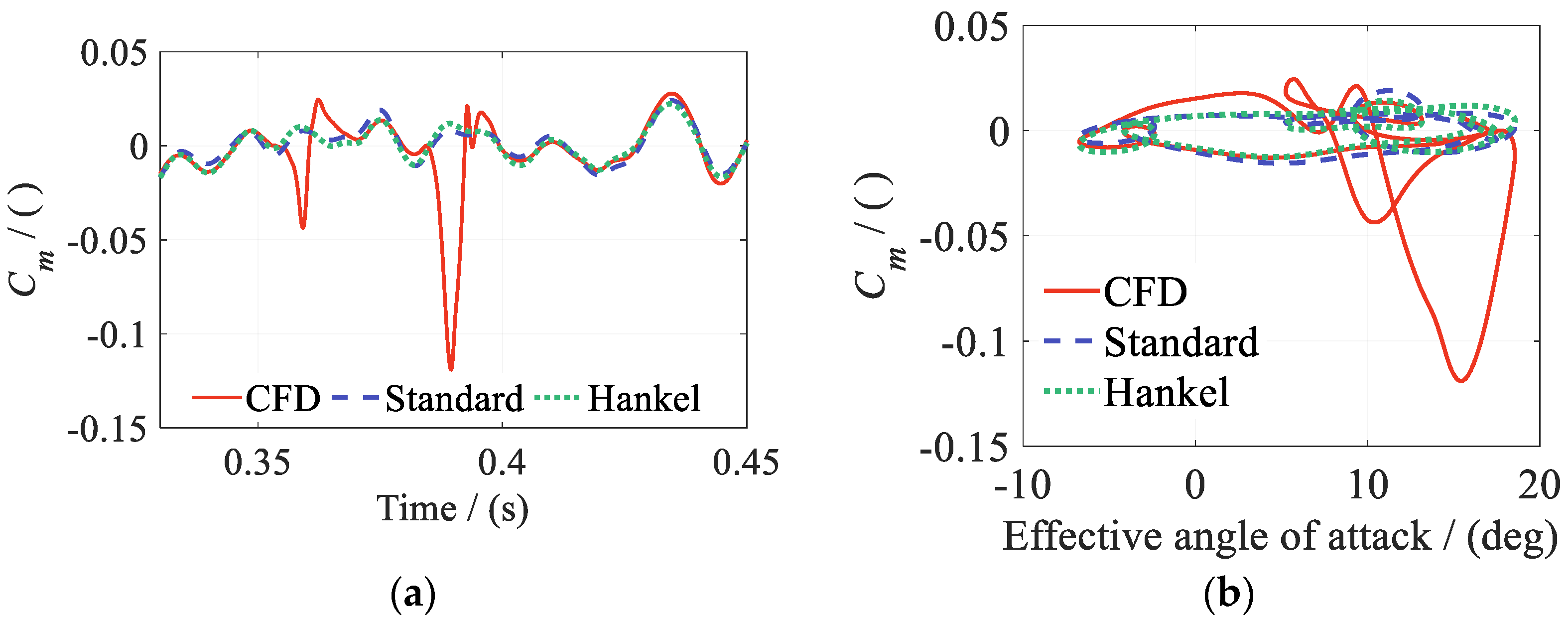
When the pitch-amplitude scaling factor increases to λα = 1.8, the overall predictions remain good. Errors increase markedly only near the maximum effective angle of attack, as shown in Figure 31, Figure 32, Figure 33 and Figure 34. This interval spans t = 0.33–0.45 s. The effective angle of attack reaches approximately 19.45° at t = 0.3860 s, as shown in Figure 31. During the subsequent pitch-down phase, after a delay of approximately 3.2 ms, the effective angle of attack is approximately 16.64°. At this point, the lift coefficient drops abruptly, the drag coefficient rises sharply, and the pitching moment coefficient undergoes an abrupt change.
Figure 31.
Angle of attack for a pitch FWGN amplitude scaling factor of λα = 1.8.
Figure 32.
Lift coefficient Cl for a pitch-amplitude scaling factor of λα = 1.8: (a) time; (b) effective AOA.
Figure 33.
Drag coefficient Cd for a pitch-amplitude scaling factor of λα = 1.8: (a) time; (b) effective AOA.
Figure 34.
Pitching moment coefficient Cm for a pitch-amplitude scaling factor of λα = 1.8: (a) time; (b) effective AOA.
Figure 32b, Figure 33b and Figure 34b plot the aerodynamic coefficients against the effective angle of attack. The hysteresis loops exhibit typical dynamic-stall characteristics. Standard DMDc and Hankel-DMDc predict the loads outside the abrupt-change interval, but neither captures the strongly nonlinear phenomenon of deep dynamic stall. Previous research [50] also shows that linear DMDc cannot adequately represent nonlinear flow when a fixed-angle airfoil enters strongly separated regimes such as deep stall. The localized errors identify an accuracy limit at this large extrapolation amplitude, even though neither ROM produces spurious spikes or numerical divergence. For future ROM/CSD coupling, the training envelope will be designed to cover the range of inputs expected during coupled simulations.
In summary, both Standard DMDc and Hankel-DMDc maintain stable long-horizon rolling prediction on inputs outside the training dataset. They predict the amplitude and phase characteristics of the aerodynamic responses well. Within λα = 0.6–1.5, both methods show good extrapolation capability and dynamic stability. The delayed state vector in Hankel-DMDc further represents memory effects, providing more stable prediction under complex coupled conditions. The independent predictions in this section used a baseline excitation signal that was not used for training. Only the pitch amplitude of this signal was varied to assess its effect on prediction performance. Since all cases were derived from a single baseline signal, prediction accuracy across multiple independently generated excitation signals remains to be verified.
4.5. Multi-ROM Blending for Wide-Mach-Range Prediction
The individual ROMs in Section 4.4 show good pitch-amplitude extrapolation capability. However, rotor aerodynamic models require a broad Mach number range, such as Ma = 0.15–0.85. To meet this requirement, this subsection constructs a blended ROM from local ROMs with overlapping Mach number training intervals. The prediction performance of the local and blended ROMs is evaluated separately for Standard DMDc and Hankel-DMDc. The method exploits the good prediction accuracy of each local ROM within its training interval. A contribution-weighting scheme enables continuous transitions between the local ROMs in the overlap region.
The two local ROMs follow the modeling procedure in Section 4.4. They differ only in the Mach number input for the time-varying freestream. As in Section 4.4, the time-varying freestream excitation is expressed as:
where the Mach number range of ROM 1 is Ma ∈ [0.2,0.4], with Ma0 = 0.30 and Ma_Amp = 0.10. The range of ROM 2 is Ma ∈ [0.3,0.5]. The two ranges overlap over Ma = 0.30–0.40. Standard DMDc and Hankel-DMDc are trained, blended, and used for prediction separately. The two methods remain independent. The Mach number variation in the validation cases is:
where the Mach number range is Ma ∈ [0.2,0.5]. To simplify the analysis, the weights of the two ROMs vary linearly in the overlap region. The weighted output is expressed as:
where denotes the aerodynamic coefficients predicted by each local ROM. w1 and w2 are the corresponding weights, which vary linearly with the instantaneous Mach number. For the Mach number ranges above, the weights are defined as:
with w2(Ma) = 1.0 − w1(Ma). Cases 1–3 are designed as independent-prediction cases to examine the applicability of the blended ROM under different unsteady-motion parameters. Each motion degree of freedom uses single-harmonic excitation to simplify the analysis and emphasize the effect of the time-varying Mach number. Relatively large motion amplitudes are selected so that the motion variables span a broad portion of the training range within one cycle. Cases 1–3 have identical plunge-displacement, pitch, and flap-deflection amplitudes and the same time-varying freestream. Only the excitation frequencies of the motion inputs are increased progressively. This tests prediction at different unsteady time scales. The motion excitations are expressed as:
where ha/b, αa, and βa denote the nondimensional plunge-displacement amplitude, main-airfoil pitch amplitude, and flap-deflection amplitude, respectively. α0 denotes the mean pitch angle. The excitation frequencies of the three degrees of freedom are fh, fα, and fβ, with corresponding reduced frequencies kh, kα, and kβ. The motion-input parameters for Cases 1–3 are summarized in Table 5.
Table 5.
Parameters of each degree of freedom for validation Cases 1–3.
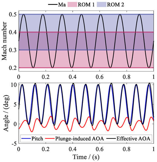
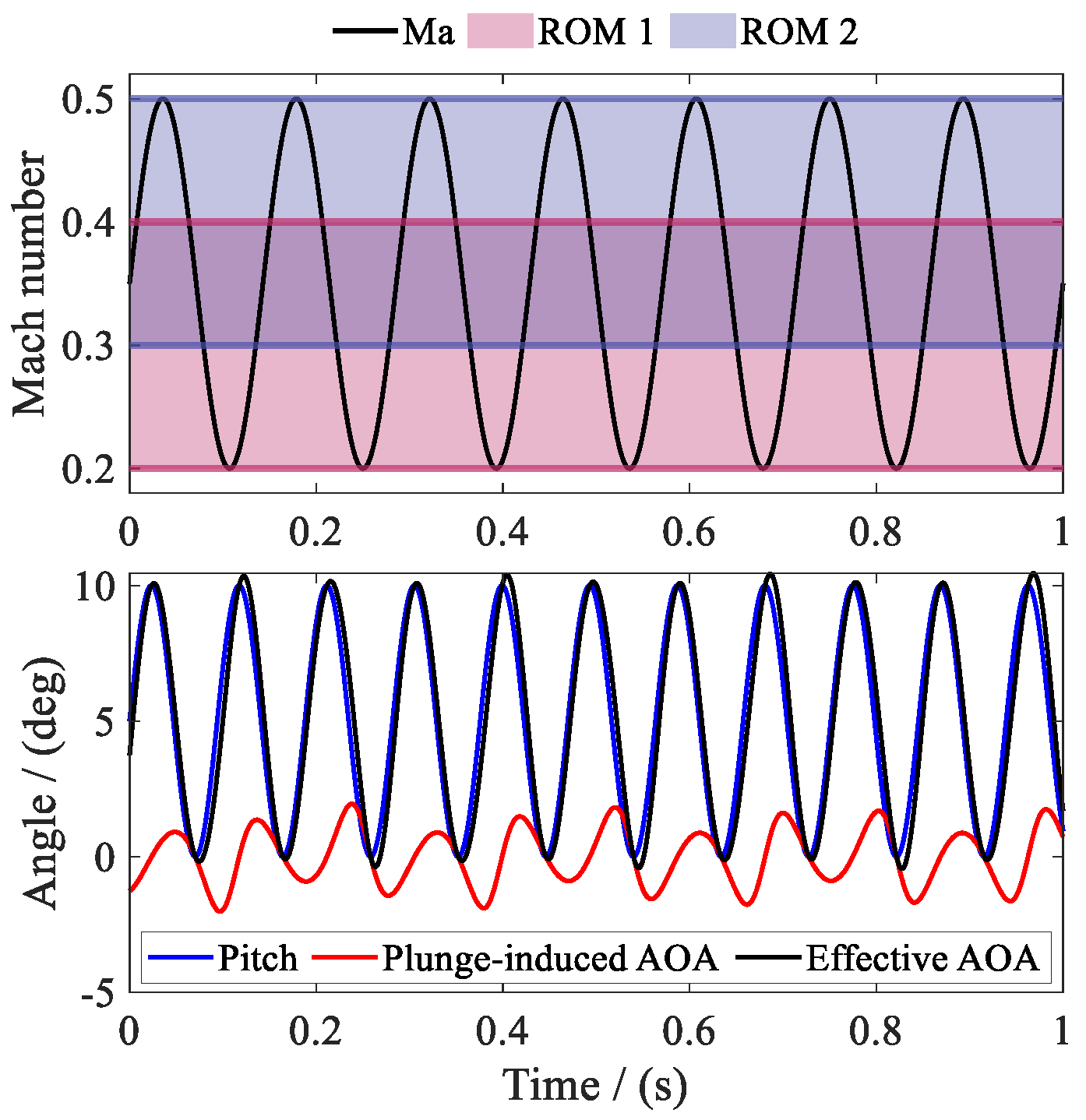
Figure 35 shows the pitch and plunge motions in Case 1 and the Mach number ranges of the two local ROMs. Within one cycle of the time-varying freestream, Ma(t) passes successively through the ROM 1-only region, the overlap region, and the ROM 2-only region. It crosses these exclusive and overlap regions repeatedly over the full time history. This case provides an effective test of the need for ROM blending and the effect of weight transitions.
Figure 35.
Freestream Mach number ranges of Case 1 and the two ROMs.
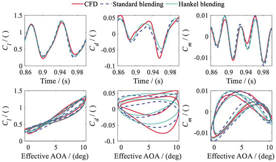
The CFD simulations for Cases 1–3 each cover t = 1.0 s. The CFD results for all cases begin to converge in the second cycle. Subsequent error statistics and plots use the last complete cycle. For computational-time comparison, all CFD cases are run with 16 threads on an AMD Ryzen 9 7950X processor with a base frequency of 4.5 GHz. Each CFD case takes approximately 11.0 h on average. Once the CFD data are available, ROM 1 and ROM 2 are constructed separately using Standard DMDc and Hankel-DMDc, giving four local ROMs. Their total offline training time is only 10.57 s. For one case, prediction with all four local ROMs takes less than 0.50 s in total. Offline training time covers construction of the four local ROMs from existing CFD data. Prediction time includes input preparation and time stepping with fixed ROM matrices to obtain the lift, drag, and pitching moment coefficients. It excludes CFD data generation, ROM construction, and subsequent blending.
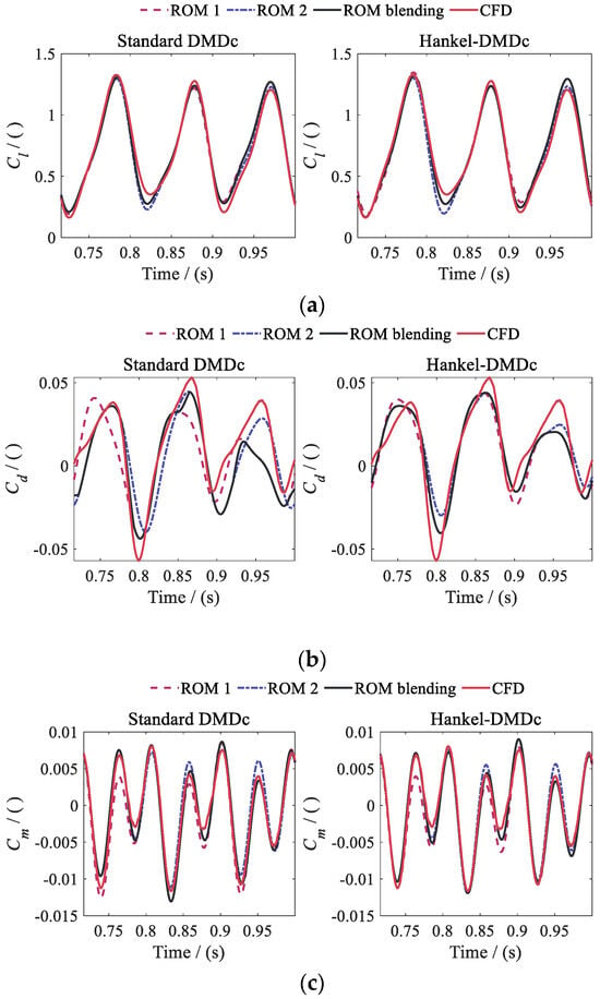
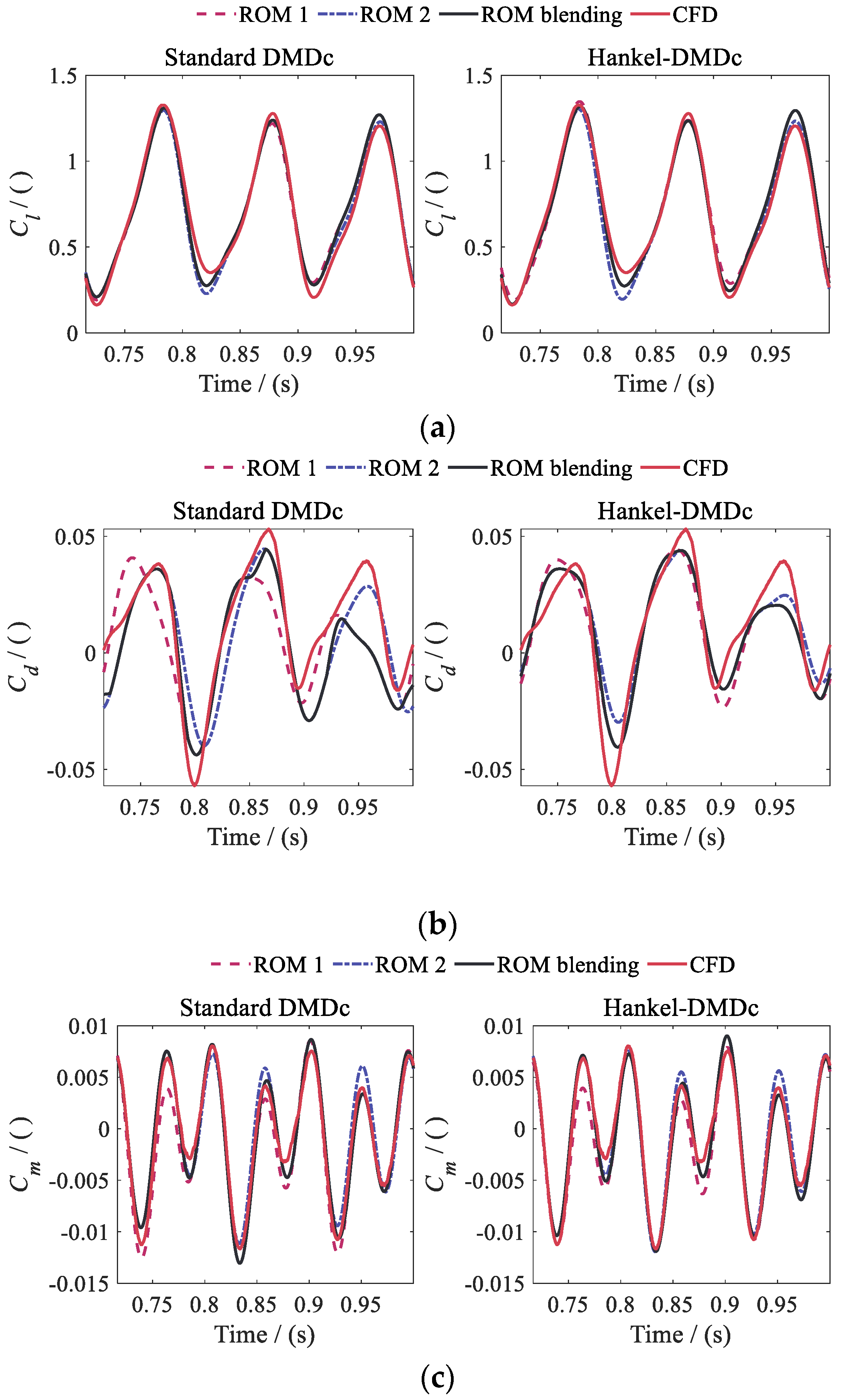
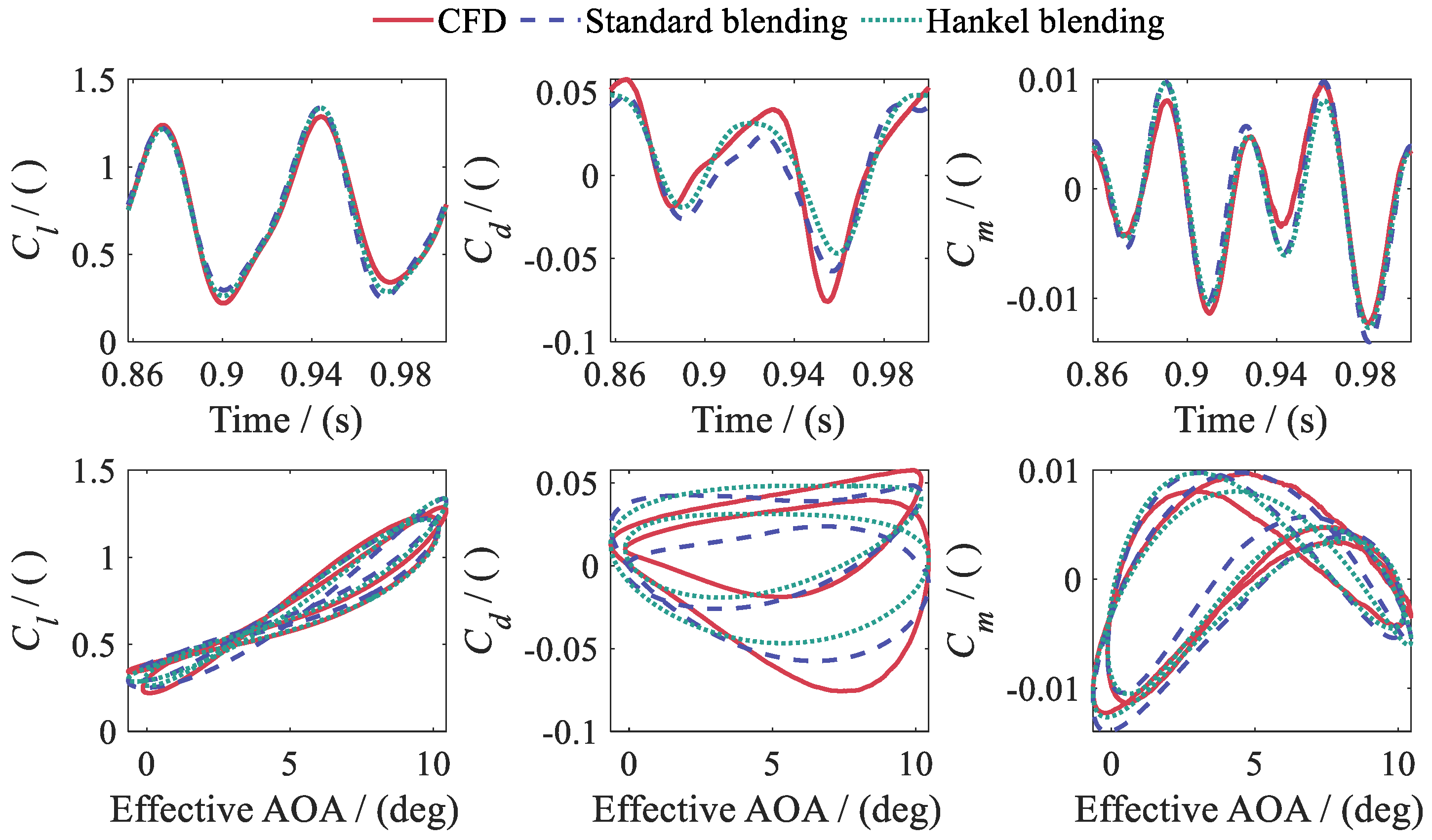
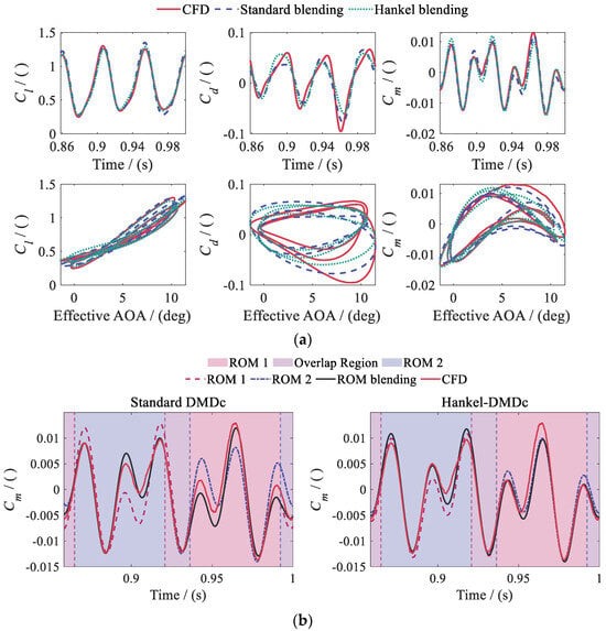
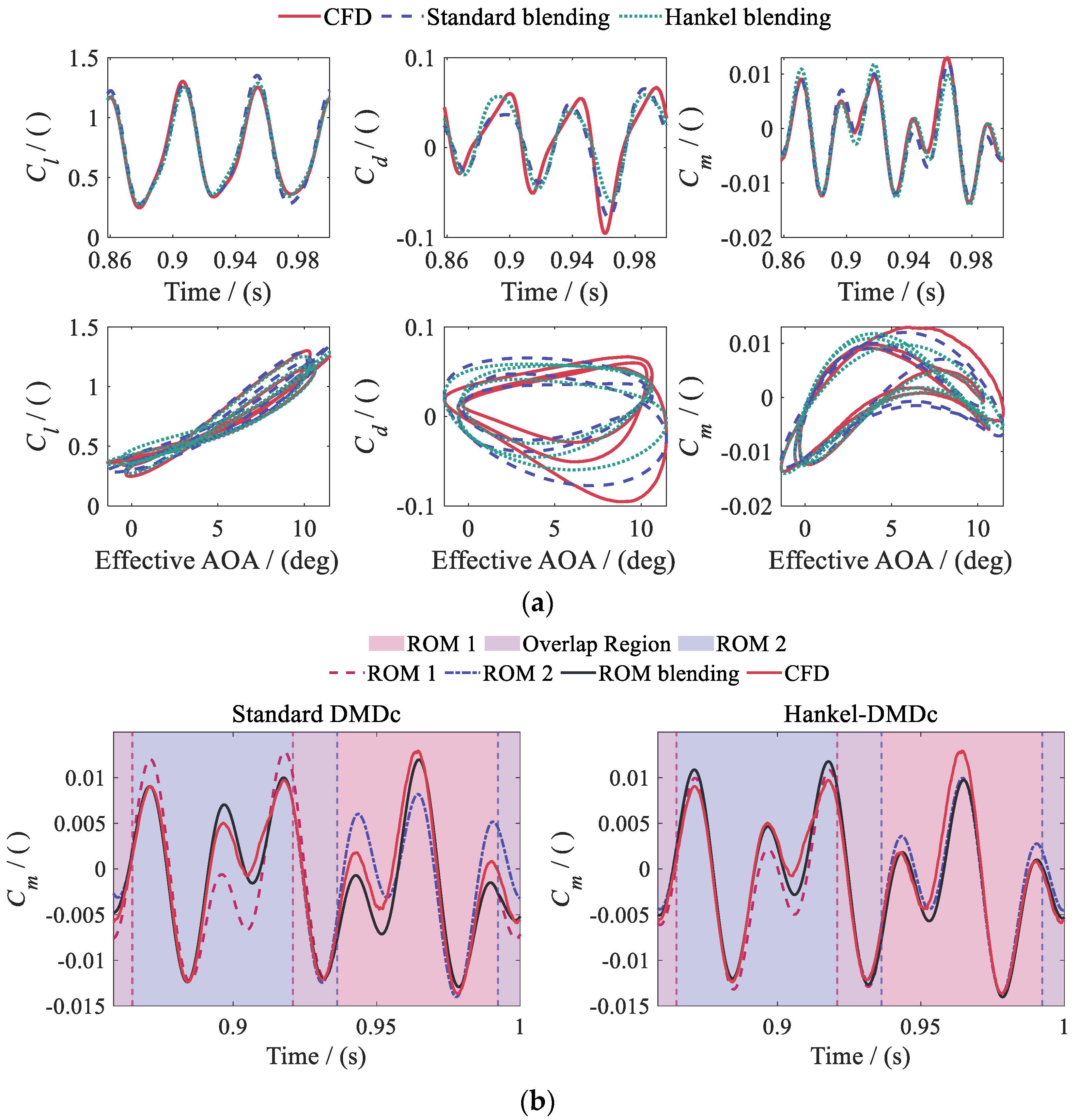
Figure 36, Figure 37 and Figure 38 use different plotting formats to present the CFD values and the predictions of ROM 1, ROM 2, and the blended ROM for Cases 1–3. Each local ROM predicts accurately within its training Mach number range. In extrapolation regions, however, some aerodynamic coefficients exhibit amplitude or phase deviations. The blended ROM continuously adjusts each local ROM’s contribution with Ma(t) in the overlap region. This provides a continuous transition between the output weights. The ROM-predicted aerodynamic coefficients satisfy the continuity and smoothness requirements over the entire Mach number range. No individual local ROM needs to extrapolate over the full range Ma = 0.20–0.50. Overall, the ROMs predict Cl and Cm well, while some prediction error remains in Cd.
Figure 36.
Predictions of the two local ROMs and the blended ROM for Case 1: (a) lift coefficient Cl; (b) drag coefficient Cd; (c) pitching moment coefficient Cm.
Figure 37.
Predictions of the blended ROM for Case 2.
Figure 38.
Predictions of the local and blended ROMs for Case 3: (a) predictions of the blended ROM; (b) pitching moment coefficient Cm.
Cases 1 and 2 show that the blended ROM avoids extrapolation by individual local ROMs and achieves good overall prediction accuracy, particularly near the peaks of the aerodynamic coefficients. Unsteady effects become more pronounced as the motion-excitation frequencies increase. The errors of the local ROMs in extrapolation regions increase further relative to the blended ROM. Blending performance therefore depends not only on the Mach number weights but also on the dynamic errors of the local ROMs and the prediction conditions.
Cm in Case 3 further illustrates an effective use of blending. Figure 38b shows that the blended ROM predicts accurately over the full Mach number range compared with ROM 1 and ROM 2. Both local ROMs exhibit prediction deviations and increased errors in their respective Mach number extrapolation regions. Table 6 summarizes the prediction errors of the two local ROMs and the blended ROM for Cases 1–3.
Table 6.
Average prediction errors for Cases 1–3.
Hankel-DMDc has smaller prediction errors than Standard DMDc. The table shows that ROM 2 has lower average prediction errors than ROM 1 for all aerodynamic coefficients. A possible reason is that the Mach number range of ROM 2 extends to higher values, so its training data contain more pronounced compressibility effects. The blended ROM generally yields lower prediction errors than ROM 1 and ROM 2. The improvement in Cm is particularly pronounced. For Hankel-DMDc, the average Cm prediction error decreases from 4.60% to 4.41%. The average Cd error of Standard DMDc decreases from 10.36% to 8.98%, and the average Cl error of Hankel-DMDc decreases from 3.51% to 2.92%. These results show that blending exploits the complementary capabilities of the local ROMs for key aerodynamic components.
Some improvements are nevertheless small. This may be because the local ROMs already have good Mach number extrapolation capability. In summary, blending local ROMs covering Ma = 0.20–0.40 and Ma = 0.30–0.50 extends the effective prediction range to Ma = 0.20–0.50. In principle, adding more local ROMs could extend the coverage to a broader range, such as Ma = 0.15–0.85, to meet the requirements for unsteady rotor aerodynamic calculations. This broader range has not yet been validated and requires further verification.
5. Conclusions
This study constructs an end-to-end DMDc-based reduced-order modeling framework for the airfoil-flap system. It maps motion and freestream inputs to Cl, Cd, and Cm. The reconstruction performance of Standard DMDc and Hankel-DMDc is examined using the same CFD training data. Independent rolling prediction, pitch-amplitude extrapolation, and extension of the Mach number envelope are then validated. The main conclusions are as follows:
- As the airfoil-system inputs expand from a single primary motion to complete-DOF inputs, the reconstruction errors of both DMDc methods remain of a similar order of magnitude. The ROMs are thus suitable for multiple-input/multiple-output (MIMO) modeling of this system.
- The delayed state in Hankel-DMDc improves prediction accuracy under strongly coupled conditions with pronounced memory effects. For the complete-DOF case, Hankel-DMDc has lower reconstruction errors than Standard DMDc. It also exhibits a shorter convergence interval from zero initial conditions.
- Within the pitch-amplitude scaling range λα = 0.6–1.5, prediction errors do not increase markedly with amplitude. The models perform more than ten thousand steps in the independent test interval without observed error accumulation or numerical divergence. This validates their long-horizon prediction stability. When larger pitch amplitudes induce deep dynamic stall, neither model accurately captures the abrupt aerodynamic-response changes. Future work will focus on improving the ROMs’ ability to identify and predict intermittent, strongly nonlinear aerodynamic responses.
- ROM blending combines the local ranges Ma = 0.20–0.40 and Ma = 0.30–0.50 into Ma = 0.20–0.50. Compared with CFD, the ROMs substantially improve computational efficiency.
The framework accommodates complete-DOF inputs, flow-field memory, rolling prediction without output feedback, and broad Mach number coverage. It provides a basis for efficient prediction of unsteady aerodynamic loads on conventional rotors and smart rotors equipped with active trailing-edge flaps, as well as for ROM/CSD coupling and vibration control. Future helicopters and rotorcraft may adopt diverse configurations. The ROM framework developed in this study offers potential for application and deployment across different configurations.
Author Contributions
Conceptualization, Z.Y.; methodology, W.W.; software, W.W.; validation, W.Y.; formal analysis, P.L.; investigation, W.W.; resources, W.Y.; data curation, W.W. and P.L.; writing—original draft preparation, W.W.; writing—review and editing, Z.Y.; visualization, P.L.; supervision, Z.Y.; funding acquisition, Z.Y. All authors have read and agreed to the published version of the manuscript.
Funding
This research was funded by the joint research project on lightweight intelligent vibration reduction of helicopter fuselage, grant number KT240, and the Special Fund of National Key Laboratory of Helicopter Aeromechanics, grant number ZAG25006-04.
Data Availability Statement
The original contributions presented in this study are included in the article. Further inquiries can be directed to the corresponding author.
Conflicts of Interest
The authors declare no conflicts of interest.
References
- Straubinger, A.; Rothfeld, R.; Shamiyeh, M.; Büchter, K.-D.; Kaiser, J.; Plötner, K.O. An overview of current research and developments in urban air mobility—Setting the scene for UAM introduction. J. Air Transp. Manag. 2020, 87, 101852. [Google Scholar] [CrossRef] [Scilit]
- Mohsan, S.A.H.; Khan, M.A.; Noor, F.; Ullah, I.; Alsharif, M.H. Towards the unmanned aerial vehicles (UAVs): A comprehensive review. Drones 2022, 6, 147. [Google Scholar] [CrossRef] [Scilit]
- Oates, B.; Su, P.; Hrynuk, J.T.; Rauleder, J.; Smith, M.J. Assessment of modeling techniques for predictions of uncrewed aerial vehicle unsteady aerodynamics. Aerosp. Sci. Technol. 2026, 176, 112496. [Google Scholar] [CrossRef] [Scilit]
- Ghoreyshi, M.; Jirásek, A.; Cummings, R.M. Reduced order unsteady aerodynamic modeling for stability and control analysis using computational fluid dynamics. Prog. Aerosp. Sci. 2014, 71, 167–217. [Google Scholar] [CrossRef] [Scilit]
- Kou, J.; Zhang, W. Data-driven modeling for unsteady aerodynamics and aeroelasticity. Prog. Aerosp. Sci. 2021, 125, 100725. [Google Scholar] [CrossRef] [Scilit]
- Leishman, J.G.; Beddoes, T.S. A semi-empirical model for dynamic stall. J. Am. Helicopter Soc. 1989, 34, 3–17. [Google Scholar] [CrossRef] [Scilit]
- Theodorsen, T. General Theory of Aerodynamic Instability and the Mechanism of Flutter; NACA Report 496; U.S. Government Printing Office: Washington, DC, USA, 1935. Available online: https://ntrs.nasa.gov/citations/19930090935 (accessed on 15 November 2026).
- Friedmann, P.P. Arbitrary motion unsteady aerodynamics and its application to rotary-wing aeroelasticity. J. Fluids Struct. 1987, 1, 71–93. [Google Scholar] [CrossRef] [Scilit]
- de Terlizzi, M.; Friedmann, P.P. Active control of vibrations due to BVI and experimental correlation. In Proceedings of the 25th European Rotorcraft Forum, Rome, Italy, 14–16 September 1999. Paper G6; pp. G6.1–G6.16. [Google Scholar]
- Myrtle, T.F.; Friedmann, P.P. Application of a new compressible time domain aerodynamic model to vibration reduction in helicopters using an actively controlled flap. J. Am. Helicopter Soc. 2001, 46, 32–43. [Google Scholar] [CrossRef] [Scilit]
- Patt, D.; Liu, L.; Friedmann, P.P. Rotorcraft vibration reduction and noise prediction using a unified aeroelastic response simulation. J. Am. Helicopter Soc. 2005, 50, 95–106. [Google Scholar] [CrossRef] [Scilit]
- Liu, L.; Padthe, A.K.; Friedmann, P.P.; Quon, E.; Smith, M.J. Unsteady aerodynamics of an airfoil/flap combination on a helicopter rotor using computational fluid dynamics and approximate methods. J. Am. Helicopter Soc. 2011, 56, 032003. [Google Scholar] [CrossRef] [Scilit]
- Padthe, A.K.; Friedmann, P.P.; Chia, M.H.; Liu, L. Comprehensive numerical assessment of rotorcraft vibration and noise control using microflaps. J. Aircr. 2016, 53, 1113–1130. [Google Scholar] [CrossRef] [Scilit]
- Chia, M.H.; Padthe, A.K.; Duraisamy, K.; Friedmann, P.P. An efficient approach for the simulation and on-blade control of helicopter noise and the impact on vibration. J. Am. Helicopter Soc. 2017, 62, 042004. [Google Scholar] [CrossRef] [Scilit]
- Dowell, E.H. Eigenmode analysis in unsteady aerodynamics: Reduced-order models. AIAA J. 1996, 34, 1578–1583. [Google Scholar] [CrossRef] [Scilit] [PubMed]
- Silva, W.A. Identification of linear and nonlinear aerodynamic impulse responses using digital filter techniques. In Proceedings of the 22nd AIAA Atmospheric Flight Mechanics Conference, New Orleans, LA, USA, 11–13 August 1997. AIAA Paper 1997-3712. [Google Scholar] [CrossRef] [Scilit]
- Ghoreyshi, M.; Aref, P.; Stradtner, M.; Panagiotopoulos, A.; van Rooij, M.; Blom, P.H.L.; Hulshoff, S. Evaluation of reduced order aerodynamic models for transonic flow over a multiple-swept wing configuration. In Proceedings of the AIAA AVIATION Forum and ASCEND 2024, Las Vegas, NV, USA, 29 July–2 August 2024. [Google Scholar] [CrossRef] [Scilit]
- Glaz, B.; Liu, L.; Friedmann, P.P. Reduced-order nonlinear unsteady aerodynamic modeling using a surrogate-based recurrence framework. AIAA J. 2010, 48, 2418–2429. [Google Scholar] [CrossRef] [Scilit]
- Glaz, B.; Liu, L.; Friedmann, P.P.; Bain, J.; Sankar, L.N. A surrogate-based approach to reduced-order dynamic stall modeling. J. Am. Helicopter Soc. 2012, 57, 022002. [Google Scholar] [CrossRef] [Scilit]
- Glaz, B.; Friedmann, P.P.; Liu, L.; Cajigas, J.G.; Bain, J.; Sankar, L.N. Reduced-order dynamic stall modeling with swept flow effects using a surrogate-based recurrence framework. AIAA J. 2013, 51, 910–921. [Google Scholar] [CrossRef] [Scilit]
- Liu, P.; Yu, G.; Zhu, X.; Du, Z. Unsteady aerodynamic prediction for dynamic stall of wind turbine airfoils with the reduced order modeling. Renew. Energy 2014, 69, 402–409. [Google Scholar] [CrossRef] [Scilit]
- Liu, H.; Hu, H.; Zhao, Y.; Huang, R. Efficient reduced-order modeling of unsteady aerodynamics robust to flight parameter variations. J. Fluids Struct. 2014, 49, 728–741. [Google Scholar] [CrossRef] [Scilit]
- Li, X.; Zheng, G.; Grecov, D.; Hou, Z. Efficient reduced-order modeling of unsteady aerodynamics under light dynamic stall conditions. Proc. Inst. Mech. Eng. Part G J. Aerosp. Eng. 2019, 233, 2419–2432. [Google Scholar] [CrossRef] [Scilit]
- Stradtner, M.; Bekemeyer, P. Nonlinear unsteady aerodynamic reduced-order modeling using a surrogate-based recurrent framework. J. Aircr. 2025, 62, 1560–1574. [Google Scholar] [CrossRef] [Scilit]
- Kou, J.; Zhang, W. An approach to enhance the generalization capability of nonlinear aerodynamic reduced-order models. Aerosp. Sci. Technol. 2016, 49, 197–208. [Google Scholar] [CrossRef] [Scilit]
- Huang, R.; Hu, H.; Zhao, Y. Nonlinear reduced-order modeling for multiple-input/multiple-output aerodynamic systems. AIAA J. 2014, 52, 1219–1231. [Google Scholar] [CrossRef] [Scilit]
- Liu, H.; Huang, R.; Zhao, Y.; Hu, H. Reduced-order modeling of unsteady aerodynamics for an elastic wing with control surfaces. J. Aerosp. Eng. 2017, 30, 04016083. [Google Scholar] [CrossRef] [Scilit]
- Huang, R.; Liu, H.; Yang, Z.; Zhao, Y.; Hu, H. Nonlinear reduced-order models for transonic aeroelastic and aeroservoelastic problems. AIAA J. 2018, 56, 3718–3731. [Google Scholar] [CrossRef] [Scilit]
- Yang, Z.; Huang, R.; Liu, H.; Zhao, Y.; Hu, H. An improved nonlinear reduced-order modeling for transonic aeroelastic systems. J. Fluids Struct. 2020, 94, 102926. [Google Scholar] [CrossRef] [Scilit]
- Yang, Z.; Zhang, Z.; Zhang, M.; He, S. Transonic buffeting control via a nonlinear aeroservoelastic model of reduced-order. Aeronaut. J. 2026, 130, 2319–2342. [Google Scholar] [CrossRef] [Scilit]
- Carloni, A.C.N.; Azevedo, J.L.F. Development of transonic unsteady aerodynamic reduced-order models using system identification techniques. arXiv 2023, arXiv:2307.09644. [Google Scholar] [CrossRef] [Scilit]
- Efrati, R.; Raveh, D.E. Multi-output auto-regressive modeling of transonic unsteady aerodynamics. In Proceedings of the AIAA SCITECH 2026 Forum, Orlando, FL, USA, 12–16 January 2026. [Google Scholar] [CrossRef] [Scilit]
- Kou, J.; Zhang, W. Layered reduced-order models for nonlinear aerodynamics and aeroelasticity. J. Fluids Struct. 2017, 68, 174–193. [Google Scholar] [CrossRef] [Scilit]
- Skujins, T.; Cesnik, C.E.S. Reduced-order modeling of unsteady aerodynamics across multiple Mach regimes. J. Aircr. 2014, 51, 1681–1704. [Google Scholar] [CrossRef] [Scilit]
- Winter, M.; Breitsamter, C. Neurofuzzy-model-based unsteady aerodynamic computations across varying freestream conditions. AIAA J. 2016, 54, 2705–2720. [Google Scholar] [CrossRef] [Scilit]
- Kou, J.; Zhang, W. Reduced-order modeling for nonlinear aeroelasticity with varying Mach numbers. J. Aerosp. Eng. 2018, 31, 04018105. [Google Scholar] [CrossRef] [Scilit]
- Li, K.; Kou, J.; Zhang, W. Deep neural network for unsteady aerodynamic and aeroelastic modeling across multiple Mach numbers. Nonlinear Dyn. 2019, 96, 2157–2177. [Google Scholar] [CrossRef] [Scilit]
- Immordino, G.; Da Ronch, A.; Righi, M. Parametric nonlinear Volterra series via machine learning: Transonic aerodynamics. J. Aircr. 2025, 62, 1504–1521. [Google Scholar] [CrossRef] [Scilit]
- Sun, C.; Tian, T.; Zhu, X.; Du, Z. Sparse identification of nonlinear unsteady aerodynamics of the oscillating airfoil. Proc. Inst. Mech. Eng. Part G J. Aerosp. Eng. 2021, 235, 809–824. [Google Scholar] [CrossRef] [Scilit]
- Candon, M.; Delgado-Gutiérrez, A.; Marzocca, P.; Balajewicz, M.; Dowell, E.H. Nonlinear aeroelastic reduced order modeling with optimized sparse multi-input Volterra kernels. AIAA J. 2025, 63, 3841–3856. [Google Scholar] [CrossRef] [Scilit]
- Candon, M.; Marzocca, P.; Dowell, E.H. Sparse identification of aeroelastic reduced-order models in transonic buffeting flow. In Proceedings of the AIAA SCITECH 2026 Forum, Orlando, FL, USA, 12–16 January 2026. [Google Scholar] [CrossRef] [Scilit]
- Candon, M.; Marzocca, P.; Dowell, E.H. Aeroelastic reduced-order model differential equations in transonic buffeting flow. AIAA J. 2026, 64, 5882–5899. [Google Scholar] [CrossRef] [Scilit]
- Pereira, J.A.F.; Camacho, E.A.R.; Marques, F.D.; Silva, A.R.R. Flapping airfoil aerodynamics using recurrent neural network. In Proceedings of the AIAA SCITECH 2024 Forum, Orlando, FL, USA, 8–12 January 2024. [Google Scholar] [CrossRef] [Scilit]
- Baldan, G.; Guardone, A. A deep neural network reduced order model for unsteady aerodynamics of pitching airfoils. Aerosp. Sci. Technol. 2024, 152, 109345. [Google Scholar] [CrossRef] [Scilit]
- Zhang, Y.; Tang, H.; Wei, L.; Zheng, G.; Yang, G. Kolmogorov–Arnold networks for reduced-order modeling in unsteady aerodynamics and aeroelasticity. Appl. Sci. 2025, 15, 5820. [Google Scholar] [CrossRef] [Scilit]
- Massegur, D.; Da Ronch, A. Recurrent graph convolutional multi-mesh autoencoder for unsteady transonic aerodynamics. J. Fluids Struct. 2024, 131, 104202. [Google Scholar] [CrossRef] [Scilit]
- Vojković, T.; Quero, D.; Jayaraj, R.; Kaiser, C.; Boskos, D.; Buchner, A.-J. Transonic buffet modeling via invariant manifolds. arXiv 2026, arXiv:2602.10363. [Google Scholar] [CrossRef] [Scilit]
- Yao, X.; Huang, R.; Hu, H. Data-driven modeling of transonic unsteady flows and efficient analysis of fluid–structure stability. J. Fluids Struct. 2022, 111, 103549. [Google Scholar] [CrossRef] [Scilit]
- Fonzi, N.; Brunton, S.L.; Fasel, U. Data-driven modeling for transonic aeroelastic analysis. J. Aircr. 2024, 61, 625–637. [Google Scholar] [CrossRef] [Scilit]
- Viguera, R.; Naramura, R.; Sasaki, Y.; Nonomura, T. Adaptive control pattern for real-time-visual-feedback flow separation control over airfoil with sparse processing particle image velocimetry and plasma actuator. Exp. Fluids 2026, 67, 37. [Google Scholar] [CrossRef] [Scilit]
- Kou, J.Q. Research on Unsteady Aerodynamic Modeling and Flow-Field Model Reduction Methods. Master’s Thesis, Northwestern Polytechnical University, Xi’an, China, 2018. [Google Scholar]
- Kou, J.; Zhang, W. Dynamic mode decomposition with exogenous input for data-driven modeling of unsteady flows. Phys. Fluids 2019, 31, 057106. [Google Scholar] [CrossRef] [Scilit]
- Zanotti, A.; Gibertini, G.; Grassi, D.; Spreafico, D. Wake measurements behind an oscillating airfoil in dynamic stall conditions. Int. Sch. Res. Not. 2013, 2013, 265429. [Google Scholar] [CrossRef] [Scilit]

Disclaimer/Publisher’s Note: The statements, opinions and data contained in all publications are solely those of the individual author(s) and contributor(s) and not of MDPI and/or the editor(s). MDPI and/or the editor(s) disclaim responsibility for any injury to people or property resulting from any ideas, methods, instructions or products referred to in the content. |
© 2026 by the authors. Licensee MDPI, Basel, Switzerland. This article is an open access article distributed under the terms and conditions of the Creative Commons Attribution (CC BY) license.