


Abstract
High-fidelity 3D compressor flow-field data are expensive, whereas 2D blade-to-blade (B2B) cascade data can provide a transferable prior. We present Q3D-GTN (Quasi-3D Graph Decomposition Transfer Networks), a graph-neural-network transfer framework that decomposes a 3D stator passage into a quasi-3D graph by stacking seven B2B sections with spanwise edges and predicts steady flow field : a 2D-pretrained in-section backbone supplies , and a lightweight, identity-initialized spanwise residual module learns from scarce 3D samples. A four-method ablation sharing one loss and one learning rate isolates each ingredient; on a stator dataset the residual method is the most accurate at every sample size, especially with small training set. Beyond accuracy, a 3D-to-2D back-reaction analysis is proposed to reveal a structured division of labor. The backbone, whose message passing is confined within sections, carries the corrections expressible from per-section conditions, while the residual module carries those requiring inter-section coupling. A radial dominance flip in the tangential-velocity correction is shown to be the imprint of this division. Together, these results elevate the “pretrained backbone + adapter” transfer learning structure into a diagnosable, predictable mechanism for cross-dimensional transfer in turbomachinery.
1. Introduction
The pursuit of high-performance compressors in modern aero-engine design calls for fully three-dimensional design, which in turn demands rapid and accurate flow-field prediction to obtain compressor performance [1]. Because experimental testing is prohibitively expensive, the preliminary design phase relies heavily on computational fluid dynamics (CFD). Yet resolving the detailed 3D flow field by CFD remains computationally intensive, owing to the complex, highly nonlinear, and strongly coupled nature of the internal flow [2,3]. Recent studies have shown that compressor flows involve strongly localized and coupled mechanisms across different spatial scales and the radial distribution of blade loading can fundamentally alter the development and even the type of compressor instability, highlighting the intrinsically spanwise-nonuniform nature of compressor aerodynamics [4,5].
Data-driven surrogate models have shown considerable promise as a lower-cost alternative for such high-dimensional, strongly nonlinear flow problems. A variety of architectures have been explored for flow-field reconstruction, from fully connected networks and vision transformers to operators tailored to physical fields. Among these, graph neural networks (GNNs) are particularly attractive for turbomachinery because they operate directly on the native CFD mesh and respect its unstructured connectivity. Pfaff et al. introduced mesh-based simulation with MeshGraphNet, establishing the encode–process–decode message-passing paradigm now widely used for mesh flow fields [6]. In turbomachinery specifically, Li et al. proposed an integrated graph deep-learning framework that reconstructs flow fields and predicts performance across blade-span sections and the blade surface, and subsequently extended graph learning to multi-fidelity data fusion and to uncertainty quantification and robust aerodynamic optimization [7,8,9]. Strönisch et al. used multiscale GNNs to predict steady and unsteady flow quantities on industry-scale turbomachinery meshes, addressing the long information-propagation distances of large graphs [10]; Blechschmidt et al. demonstrated rapid approximation of 3D compressor flow solutions with GNNs [11]. Physics-informed graph approaches have also been brought to compressor cascades, including under unbalanced data [12,13]. These works confirm the maturity of GNN flow-field surrogates; they are, however, predominantly single-dimension models trained end-to-end, and they do not exploit the 2D-to-3D physical structure of the compressor design process.
Compressor flow modeling is further constrained by data economics: the design space is large, and each labeled 3D sample requires an expensive high-fidelity simulation. Surrogates are therefore routinely trained on sparse 3D data, with accuracy too low for the resulting performance predictions to be usable in design. Extracting transferable structure from limited samples—so that the flow field can be reconstructed and aerodynamic performance extrapolated into unexplored regions of the parameter space—is a central challenge for deep-learning models of compressors.
Conventional compressor design offers a template. Three-dimensional, strongly coupled blade design has long been approached by iteratively solving stream surfaces and performing stage-element modeling—building the high-dimensional design on a lower-dimensional, data-rich foundation [1,2]. This mirrors transfer learning, which adapts a model trained on a data-rich, lower-dimensional source domain to a data-scarce, higher-dimensional target domain. Among transfer strategies, network-based approaches—reusing part of a pretrained network and adding new components for the target task—are the most common and effective. Transfer learning has accordingly been adopted across aerodynamics: Subel et al. pretrained on low-Reynolds-number, low-resolution turbulence and transferred to high-Reynolds-number, high-resolution fields [14]; Liu et al. constrained the transfer direction via a minimum-energy-path formulation, validated on shock/boundary-layer interactions and airfoil boundary layers [15]; Wang et al. proposed a general deep transfer framework predicting airfoil flow fields from small data [16]; and multi-fidelity transfer has been used to build accurate surrogates from inexpensive low-fidelity data [17]. Most relevant to the present work are cross-dimensional transfers: Li et al. transferred knowledge from 2D supercritical airfoils to 3D transonic swept wings [18], and Yang et al. developed physics-embedded transfer models predicting swept-wing aerodynamics from airfoil data [19].
There are two gaps remaining. First, the cross-dimensional studies above target external aerodynamics and transfer at the level of the whole network or its features. For compressors, whose internal flow admits a natural quasi-3D decomposition into blade-to-blade sections plus spanwise coupling, with the latter becoming particularly important when radial loading redistribution, vortex transport, and inter-passage interactions are involved [20,21], an architecture that mirrors this decomposition—and thereby assigns the pretrained 2D operator and the new 3D components distinct, physically meaningful roles—has not been established. Second, the “pretrained backbone plus lightweight adapter” paradigm is used across all of these works as an empirical method, but how the pretrained component and the added component divide the target-domain task between them, what property of the data governs that division, and how the division evolves with the amount of target data remain unexamined. Without answers, practitioners cannot predict—for a new physical quantity, a new flow region, or a new sample budget—whether transfer will help, which component will carry the load, or how much 3D data is enough.
This paper addresses both gaps on a transonic compressor stator, using a GNN transfer framework (Q3D-GTN) that decomposes the 3D passage into a quasi-3D graph of seven blade-to-blade sections stacked with spanwise edges, and predicts : the 2D-pretrained backbone supplies on each section, and a lightweight, identity-initialized spanwise residual module learns . The contributions of this study are:
(1) A quasi-3D residual transfer method with a clean four-way ablation. The in-section operator pretrained on 2D cascade data is reused directly on the quasi-3D graph, while 3D coupling is carried exclusively by the spanwise residual module. A four-method ablation (from-scratch training, full fine-tuning, frozen transfer, and the residual method) shares one loss and one learning rate, so that each architectural ingredient—the 2D prior, the residual structure, and backbone adaptation—is isolated by a single controlled difference.
(2) A mechanistic account of the transfer: the backbone–residual division of labor. Through a 3D-to-2D back-reaction analysis with a comparison, we show that the two components divide the target task in a structured way: the backbone—whose message passing is confined within sections—carries the corrections expressible from per-section conditions, while the spanwise residual module carries the corrections requiring inter-section coupling. This division is enforced by the architecture’s information pathways, is strongest when 3D data are scarcest, and dissolves as samples accumulate.
(3) A data-side criterion and evaluation for cross-dimensional transfer. Using a network-independent probe, we quantify the within-section learnability of each aerodynamic quantity’s 3D correction and show that, in the scarce-data regime, the share of the task carried by the residual module is strongly anti-correlated with this learnability. Supporting all quantitative claims, we introduce an evaluation protocol for fixed-inflow datasets that exposes failure modes which the conventional relative-L2 error conceals.
The remainder of the paper is organized as follows. Section 2 describes the dataset, the 2D-pretrained GNN backbone, the quasi-3D residual transfer architecture, the four-method ablation design, and the diagnostic tools. Section 3 presents the results in four steps: the evaluation protocol and sample efficiency of the four methods; the back-reaction analysis and the controlled discovery of the backbone–residual division of labor; its architectural origin in the information pathways of the quasi-3D graph; and the quantitative link between the division and the within-section learnability of the data. Section 4 concludes.
2. Method
2.1. Dataset
2.1.1. Three-Dimensional Stator
The stator researched in this study is the stator of a compressor stage designed by our research group. Some design parameters are given in Table 1 and the meridional view is shown in Figure 1. Our previous study [13] focuses on the 2D cascade flow field prediction under unbalanced data and the geometry parameter of profiles is consistent with the blade section in this study.
Table 1.
Design parameters of compressor stage.
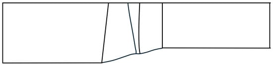
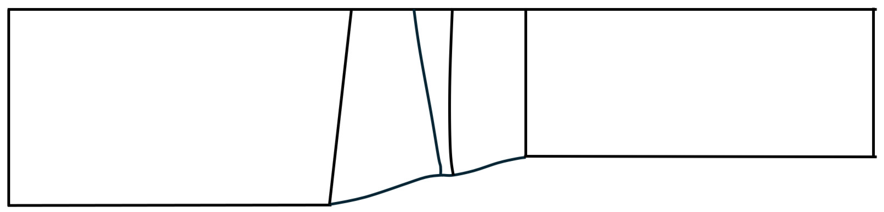
Figure 1.
Meridional view of compressor stage and its flow channel.
2.1.2. Generation and Sampling of Stator Geometry
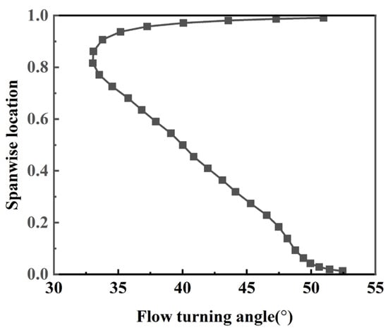
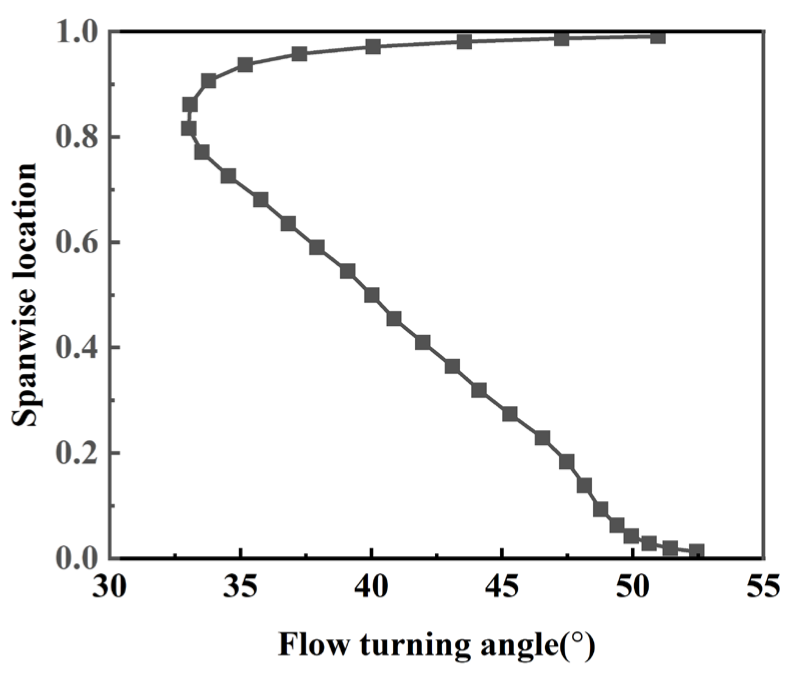
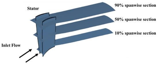
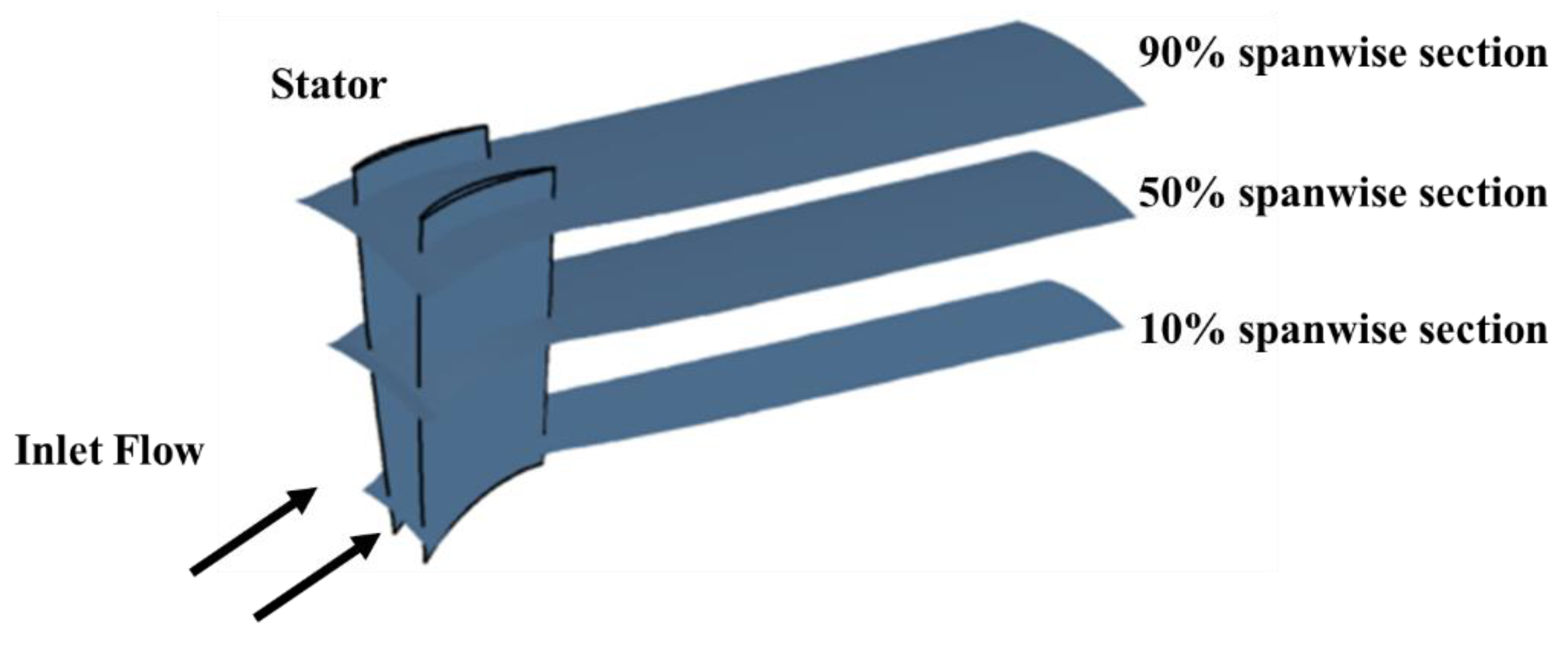
The generation of compressor stator geometry is achieved by modifying the blade sections at [10%, 20%, 30%, 50%, 70%, 80%, 90%] spanwise location. Figure 2 shows the spanwise flow deflection distribution. By analyzing the flow field at design condition and geometry of original compressor, the width constraints are given, and the ranges of camber angle at different blade sections could be determined with an estimation of deviation angle base on the simulation of original compressor stage, which are shown in Table 2.
Figure 2.
Spanwise flow deflection distribution of compressor stator.
Table 2.
Width and range of camber angles at different spanwise location.
The profile geometries are randomly extracted from the database in our previous study [13] to generate a new stator by a stacking law, which gives a fixed axial location since the axial lengths of blade sections are nearly identical with no sweeping. A deep learning model, which is a 7-layer network, is built to predict the performance of 2D cascades with different geometries to support the design afterwards. The blade profile geometry is described by a chord line and a distribution of thickness, which are both Bezier curves. The blade sections at 120% and −10% spanwise locations are identical with those at 90% and 10% spanwise locations. The stagger angles are adjusted to guarantee that the incidence angles are within [−3°, +3°]. By random sampling, a database with 500 stator geometries is built and the numerical simulations are calculated subsequently. The geometry and some blade sections of a sample in the database are shown in Figure 3.
Figure 3.
Compressor stator and sections at different spanwise locations.
2.1.3. Numerical Methods
Simulations are performed by commercial flow solver NUMECA FINE-Turbo EURANUS. The Reynolds-averaged Navier–Stokes simulations use shear stress transport (SST) as turbulence model. The inlet total temperature is 288.15 K and total pressure is 101,325 Pa. The operating condition is changed by adjusting the outlet static pressure with radial equilibrium and inlet flow is axial. The independency of the performance on mesh parameters is verified to guarantee the numerical simulations are reliable.
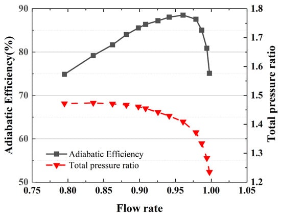
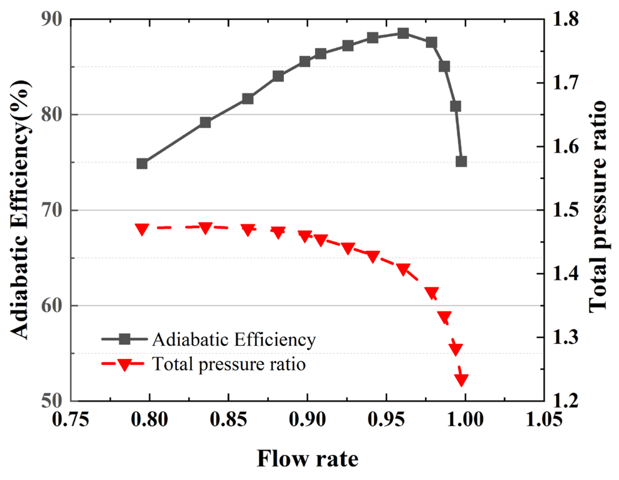
Although the topology of blade-to-blade surface in 3D mesh is fixed to be consistent with 2D cascade, the mesh refinement is performed to make sure it is dense enough. After the grid-independence verification, a mesh of 1.16 × 10⁶ cells was finally selected as the computational mesh for the 3D compressor in this study, and the isentropic efficiency and total pressure ratio characteristics are shown in Figure 4.
Figure 4.
Efficiency and total pressure ratio characteristic of compressor.
2.1.4. Partition of Dataset
The main purpose of this study is to address the limited sample problem for the training of deep learning model. Therefore, the dataset is divided into a relatively small training set, which has 20 samples and accounts for 4% of the entire dataset, and a test set which has 150 samples. The models in this paper refer to those trained under this dataset partition unless otherwise specified. Table 3 gives this and two other partitions of dataset which are utilized to verify the effectiveness of transfer learning by comparing the models trained under them. stands for the number of samples.
Table 3.
Dataset partitions.
The present validation is limited to held-out stator geometries within the same design family under a fixed imposed operating setup. Variations in local sectional conditions associated with spanwise position or geometry changes do not constitute an independent operating-condition sweep. Generalization to independently varied operating conditions has not been assessed.
2.2. GNN Backbone and Quasi-3D Graph
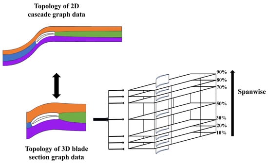
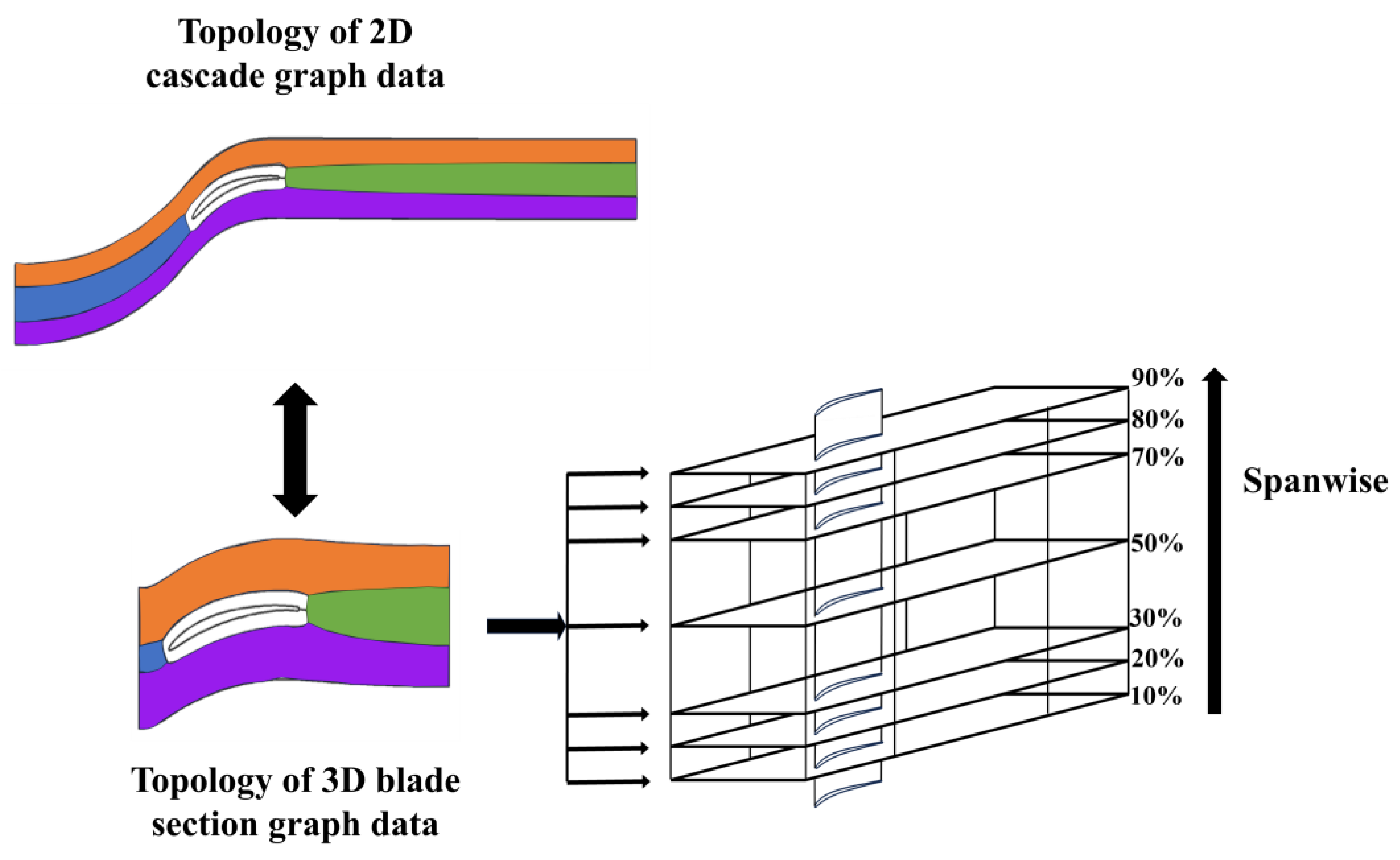
We use a GCN-based network as backbone model, which is used in 2D cascade flow field prediction in our previous study. Four flow quantities are predicted ). 3D flow field in this study is a 7-layer graph data which is constructed by stacking blade-to-blade flow surfaces of different blade sections. In each layer, the topology of graph data is identical with 2D cascade graph data. The corresponding nodes in two mutually adjacent layers are connected by edges. A 3D graph data with 59,584 nodes and 396,480 edges is utilized in this study and its correlation with 2D graph data is shown in Figure 5. For the convenience of display, blade sections are 2D rectangles, which are actually 3D curved surfaces.
Figure 5.
Topology of 2D (cascade) and 3D (compressor stator) graph data.
Each of the seven sections contains 8512 nodes with identical mesh topology and consistent node indexing. Nodes are matched between sections by mesh index, without requiring identical physical coordinates. Bidirectional spanwise edges connect matching nodes on immediately adjacent sections only. Excluding self-loops, each interior-section node has two spanwise neighbors, while nodes on the first and last sections have one. The graph contains 234,752 directed in-section edges and 102,144 directed spanwise edges (6 × 8512 × 2). Adding 59,584 self-loops gives the reported total of 396,480 edges. The backbone and residual branch use the in-section and spanwise connections, respectively.
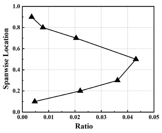
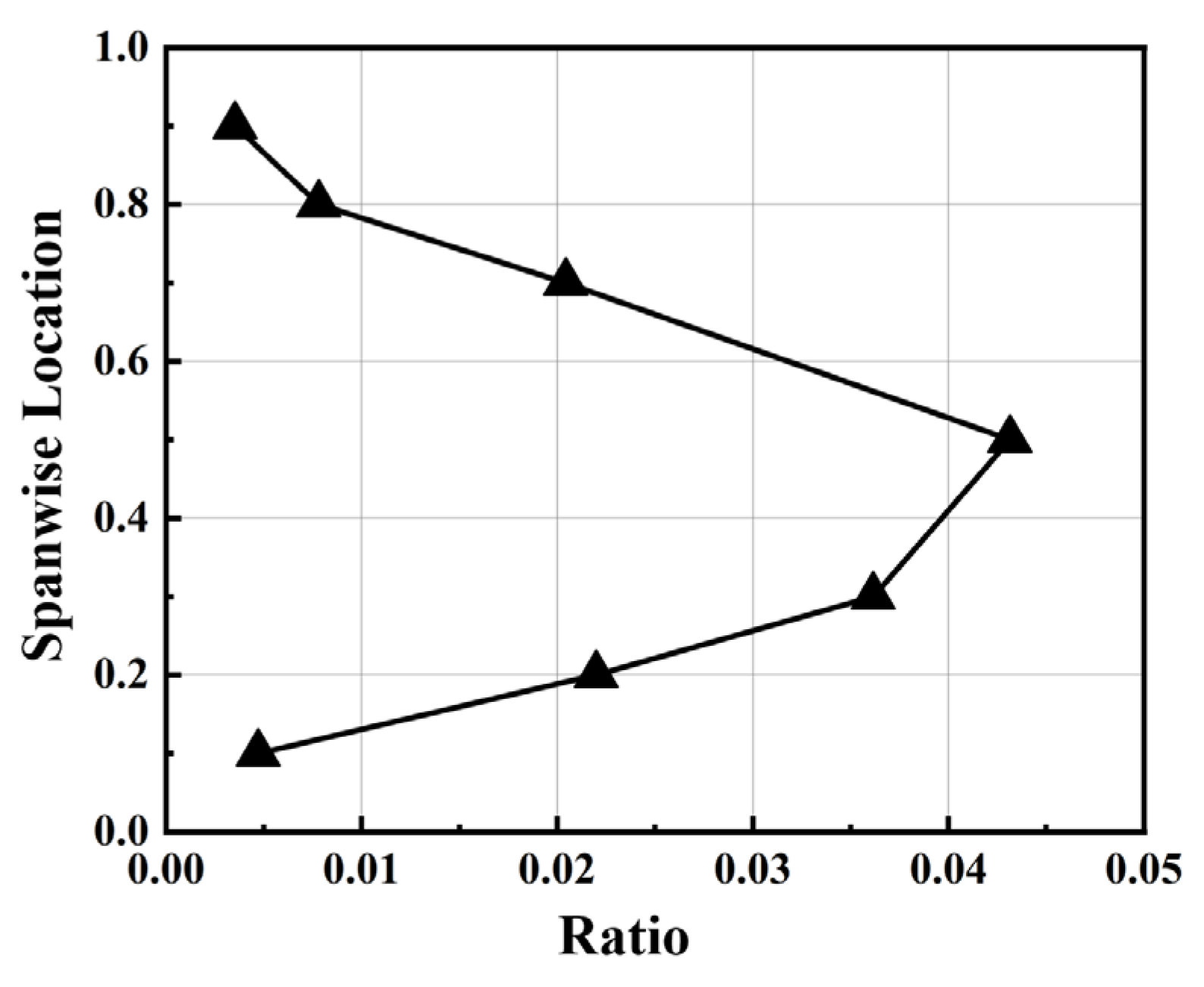
The foundation of transfer learning from 2D cascade to 3D stator blade is their similarity. First, the blade-to-blade topology of 3D data is identical with 2D data although their geometries are different. Second, the inlet flow of 3D stator is circumferential uniform due to the rotor-stator interface is mixing plane in simulations, which is consistent with 2D simulations. Finally, Figure 6 shows the average angle between flow direction and blade section and is lower than 2.5 degree which suggests that the flow direction is basically parallel with the blade section at different spanwise locations.
Figure 6.
Ratio of the velocities perpendicular and parallel to blade sections at different spanwise locations.
2.3. Residual Operator Transfer
Stage A—2D pretraining. The backbone is pretrained on the 2D cascade data and gives a transferable in-section operator which as has been done in [13].
Stage B—residual transfer. 2D and 3D have different inlet stagnation conditions, so 3D physical quantities are rescaled section-by-section onto the 2D reference while their labels and predictions share one normalized space, and evaluation rescales back to 3D physical units. On the quasi-3D graph the backbone extracts inflow conditions and decodes the operator baseline . A lightweight residual network with message passing over the spanwise edges and a residual head then produces the 3D correction , and the prediction is
The residual head is zero-initialized, so initially and : the residual starts from the identity and training can only improve on it while residual connections are carried by all extended networks.
The backbone contains four in-section GCN layers of width 128, and a three-layer MLP. The added residual branch contains two spanwise GCN layers of width 128, a 128–16–128 adapter, and an output head. Their parameter counts are 205,956 and 54,660; thus, the residual branch represents 20.97% of the full model. Both components are trainable in Finetuned Q3D, whereas the backbone is frozen in Frozen 2D. The residual head is zero-initialized, so initially and : the residual starts from the identity and training can only improve on it while residual connections are carried by all extended networks.
2.4. Four-Method Ablation
2.4.1. Architecture of Models
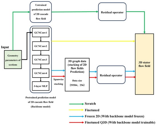
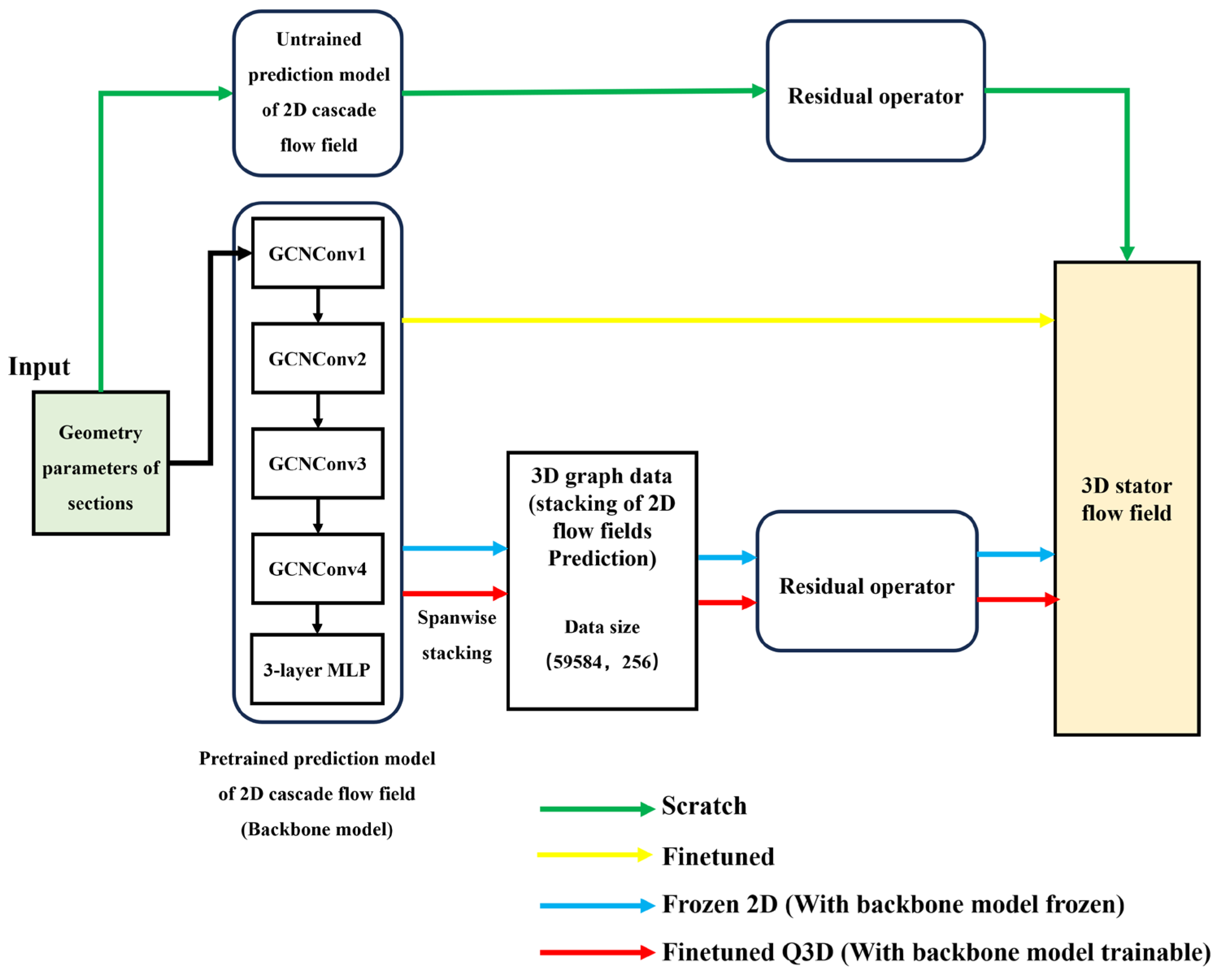
All four methods share the same components and parameter budget. They differ only in the 2D backbone which is shown in Table 4 and the data-flows of different methods are plotted in Figure 7.
Table 4.
Structures of different methods.
Figure 7.
Data-flow comparison of the four configurations.
To verify the effectiveness of the model’s transfer learning and the choice of which parameters to freeze, the following comparisons are made in the ablation study:
- Scratch vs. others: shows the effectiveness of transfer.
- Finetuned vs. Finetuned Q3D: shows the effectiveness of the residual structure.
- Frozen 2D vs Finetuned Q3D: shows the effectiveness of trainable backbone.
All four principal models share the same backbone architecture and backbone parameter count. In additional capacity tests, increasing the parameter counts of Scratch and Finetuned to approximately match those of Frozen 2D and Finetuned Q3D yielded little improvement in prediction accuracy. To ensure identical initial predictions among the transfer-based models, we used the same backbone architecture and pretrained weights, with the final linear layer of each residual output head initialized to zero.
2.4.2. Loss and Optimization
Equation (2) gives the loss of flow field prediction model and stator performance prediction model.
where is the number of nodes, . All models are trained for 5000 epochs while the learning rate decay strategy is cosine annealing. Initial learning rate is for all models.
We compared the results of three learning rates in Table 5 (, , ), as well as the results of different training epochs. It can be seen that 5 × 10⁻⁴ is the optimal hyperparameter for all architectures. Possibly, after improving the sweeping resolution, each architecture will have a better learning rate. However, this study did not conduct a more in-depth exploration in this regard. The model performance converges after 5000 training epochs, and due to the learning rate decay, the model’s prediction accuracy basically no longer changes. Across all training runs, the validation and test sets remained fixed, mutually disjoint, and separate from the training data, and all hyperparameters were selected exclusively based on validation-set performance.
Table 5.
Learning-rate screening at N = 20.
2.5. Diagnostic Tools
Accuracy is not a comprehensive metric which shows if the transferred model works but not how. There are three questions to be answered in transfer learning modeling of 3D compressor: which component absorbs the 2D-to-3D correction, whether 3D training reshapes the pretrained operator, and why this differs across quantities and spanwise locations. To address these problems, three post-hoc diagnostics were conducted and the tools used are introduced as follow.
2.5.1. 3D-to-2D Back-Reaction Analysis
Let be the original 2D backbone output and the backbone output extracted from a transferred model. Running on identical quasi-3D inputs isolates the weight change: . The percentage by which 3D training modified the 2D operator at section k and variable v is:
Plotting the spanwise distribution of localizes the adaptation along the span. The comparison of Finetuned (no residual) and Finetuned Q3D with same training samples and strategy reveals where and how strongly 3D training reshaped the 2D backbone operator.
2.5.2. Within-Section Learnability Probe
This probe utilizes ridge regression to measures how much of the true 3D correction is predictable from within-section information which is deliberately unrelated to the GNNs. Features are exactly what the backbone can access in a section: operating conditions (Mach, incidence), blade-geometry parameters, and in-section nodal coordinates.
Node-level features and targets are assembled per spanwise zone (hub 10–30%, mid 50%, tip 70–90%). The score is the held-out cross-sample : high positive values mean the correction is determined by section conditions while low or negative values mean it is not recoverable from section conditions and 3D effects from neighborhood sections are essential.
2.5.3. Division-of-Labor Measurement
From the explicit decomposition , the residual share over a variable–zone cell is defined on magnitudes:
averaged over nodes and test samples. This ratio is insensitive to the local magnitude of the total correction and shows the division of labor between backbone and residual operator.
3. Results and Discussion
3.1. Effectiveness and Sample Efficiency of Transfer Learning
3.1.1. Evaluation Metric
Since the test case is a single compressor stator and only blade geometry vary across samples while the inflow is fixed, the 3D samples share a large amount of flow structure and the relative L2 error—which is commonly used in evaluation of flow field prediction—systematically overstates the performance of model. To quantify this effect, the mean flow field of the training set is used as a fixed prediction for every test sample and attains per-variable test relL2 of 1.18% (), 1.41% (), 5.13% (), and 10.73% (). This accuracy comes entirely from shared structure and does not indicate that inter-sample differences have been learned.
We therefore adopt the mean field as the baseline and use a cross-sample normalized error as the primary metric. The error is normalized by the inter-sample standard deviation, equivalent to the cross-sample coefficient of determination while . On this scale the mean-field predictor corresponds to NRMSE = 1 and a model must fall clearly below 1 to have learned inter-sample variation. As a further reference, a predictor overfitted to a single sample attains relL2 of only 8.89% yet its cross-sample , i.e., about 3.7 times worse than not learning at all. This exposes the misleading nature of relL2 on this dataset and simultaneously confirms that substantive inter-sample differences exist to be learned.
3.1.2. Sample Efficiency of Four Methods
We first verify the effectiveness of transfer learning with 20 training samples. Table 6 reports the cross-sample NRMSE per variable of the four methods on the held-out test set. In this table, NRMSE = 1 corresponds to the non-learning mean-field baseline and values below 1 indicate that inter-sample variation has been learned.
Table 6.
Cross-sample NRMSE at N = 20 (mean-field baseline = 1).
The effectiveness of transfer learning is established in three ways. First, Scratch model remains at or above the baseline on four variables even with 20 samples—on , its prediction is worse than the non-learning baseline, and only on does it barely cross below (0.83). Second, both transfer-initialized, backbone-adaptive methods (Finetuned, Finetuned Q3D) sit clearly below the baseline on every variable which suggests that the 2D prior converts the model into an effective predictor across the board. Third, Finetuned Q3D is uniformly the best, and its margin over Finetuned is directly attributable to the spanwise coupling that module captures. Frozen 2D, by contrast, hovers near the baseline on . With the backbone locked, its residual module must bridge the entire 2D-to-3D correction alone and is overloaded.
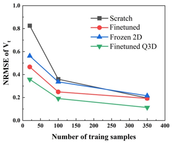
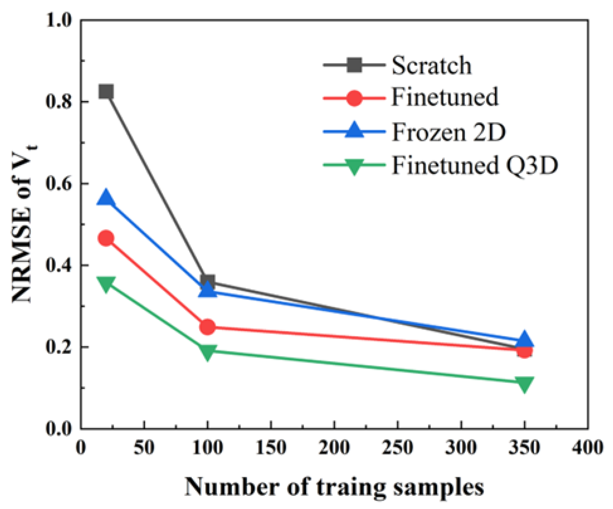
Figure 8 then examines how these conclusions depend on the data budget, plotting the NRMSE—the most discriminative variable—of all four methods against the training-set size , with the mean-field baseline marked at 1. Generating one 3D CFD sample requires approximately 5 CPU·h, whereas one 2D sample requires 0.02 CPU·h. In the comparison shown in Figure 8, Finetuned Q3D, using approximately 14,000 2D samples for backbone pretraining and 100 3D training samples, achieves a lower Vt NRMSE than Scratch trained on 350 3D samples. The corresponding CFD data-generation costs are approximately 780 CPU·h and 1750 CPU·h, respectively, representing a reduction of approximately 55%. Furthermore, the 2D cascade database could be reused for backbone pretraining in other compatible blade-flow prediction tasks. Amortizing its generation cost across multiple applications could provide additional computational savings.
Figure 8.
Sample efficiency of four methods on .
The trends sharpen the effectiveness result into a sample-efficiency statement. In the scarcest regime (N = 20), Scratch lies at 1.18—worse than not learning at all. With no prior and no structural constraint, 20 samples induce overfitting whose learned corrections are harmful on unseen samples and the normalized protocol identifies it as negative learning. The two transfer methods, in contrast, are already below the baseline at N = 20 (Finetuned 0.66, Finetuned Q3D 0.55) and improve steadily with N. Finetuned Q3D holds the best accuracy at every budget. Reading the curves horizontally, Finetuned Q3D at N = 20 already matches what Scratch cannot reach even at N = 100—the 2D prior together with the residual structure is worth several-fold the 3D data. Frozen 2D slightly superior to the baseline at N = 20, confirming that freezing wastes much of the prior’s value.
In summary: (i) transfer is what moves the model from unusable to usable—without it, small-sample training is not merely inaccurate but counterproductive; (ii) the residual module adds a consistent, cleanly attributable margin at every budget; (iii) the backbone must adapt rather than freeze. These three facts raise the mechanistic questions of what each component actually learns, which the remainder of Section 3 answers.
3.2. 3D-to-2D Back-Reaction and the Discovery of the Division of Labor
3.2.1. A Radial Dominance Flip Unique to Vt
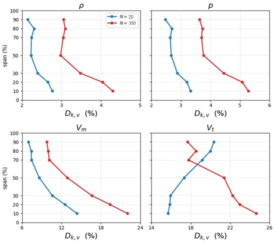
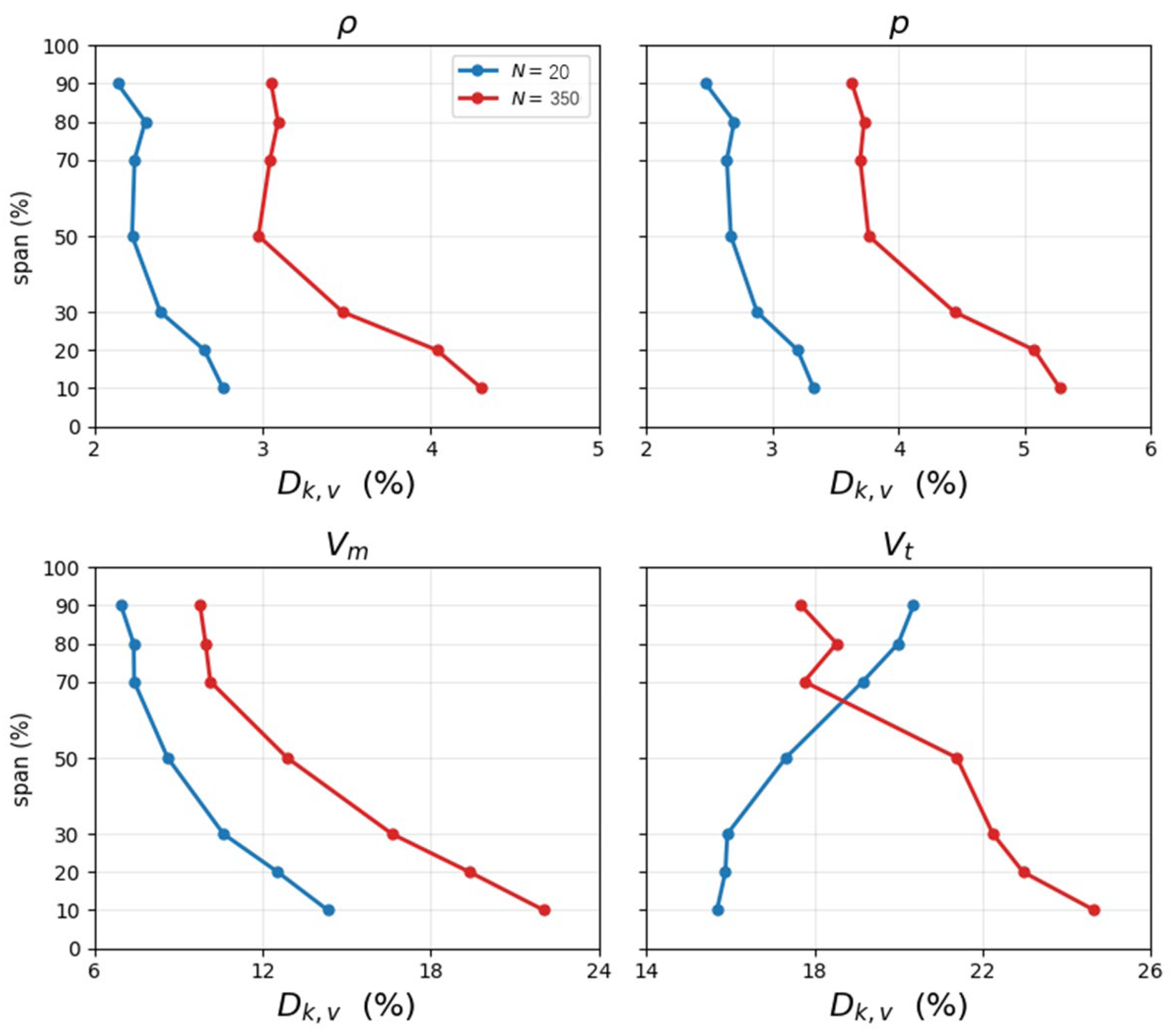
We extract the backbone without the residual module from Finetuned Q3D and run it forward on the same 3D inputs alongside the original 2D backbone to see the back-reaction of 3D effects. The magnitude of their output difference , as a percentage of the 2D-prediction magnitude, is the imprint that 3D training leaves on the 2D operator. Along the span, the four aerodynamic quantities exhibit sharply different patterns.
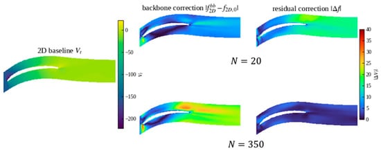
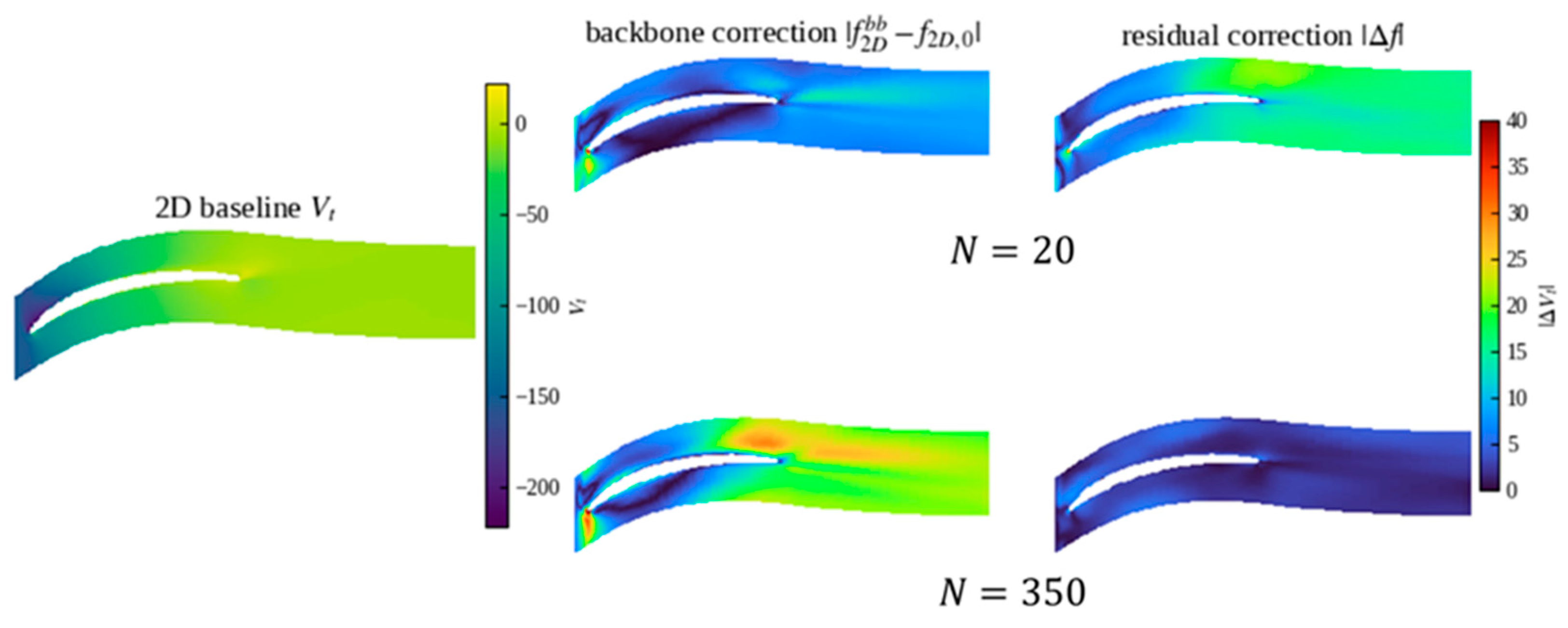
Figure 9 shows the 3D-to-2D back reaction at different spanwise locations for Finetuned Q3D model. For , decreases monotonically from hub to tip, and this radial shape is invariant to the sample size—increasing N from 20 to 350 merely scales the magnitude. Only flips its radial shape with sample size: at N = 20 the change concentrates at the tip (smallest at the hub), while at N = 350 it shifts to the hub, rejoining the pattern of the other variables.
Figure 9.
of four properties for Finetuned Q3D model with N = 20 and N = 350.
3.2.2. Controlled Comparison: The Flip Stems from Labor Division
There are two possible explanations. First, the inter-sample information of the hub correction is not extractable at small N, so the backbone can only pile its correction onto the extractable tip. Second, the information is extractable, but the joint architecture of Finetuned Q3D assigns the hub correction to the residual module, and the backbone yields accordingly. Under the former explanation, removing the residual module should leave the backbone equally flipped while removing the residual should restore the normal shape under the later one.
Using the Finetuned model as the control, we compare the radial distributions of the two backbones under the identical protocol in Table 7.
Table 7.
of backbones for different models and numbers of training samples.
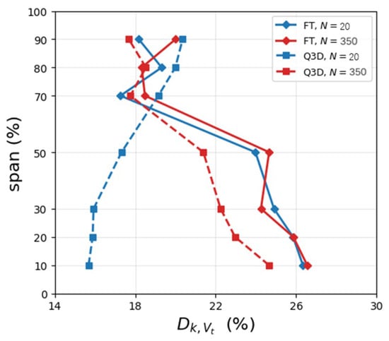
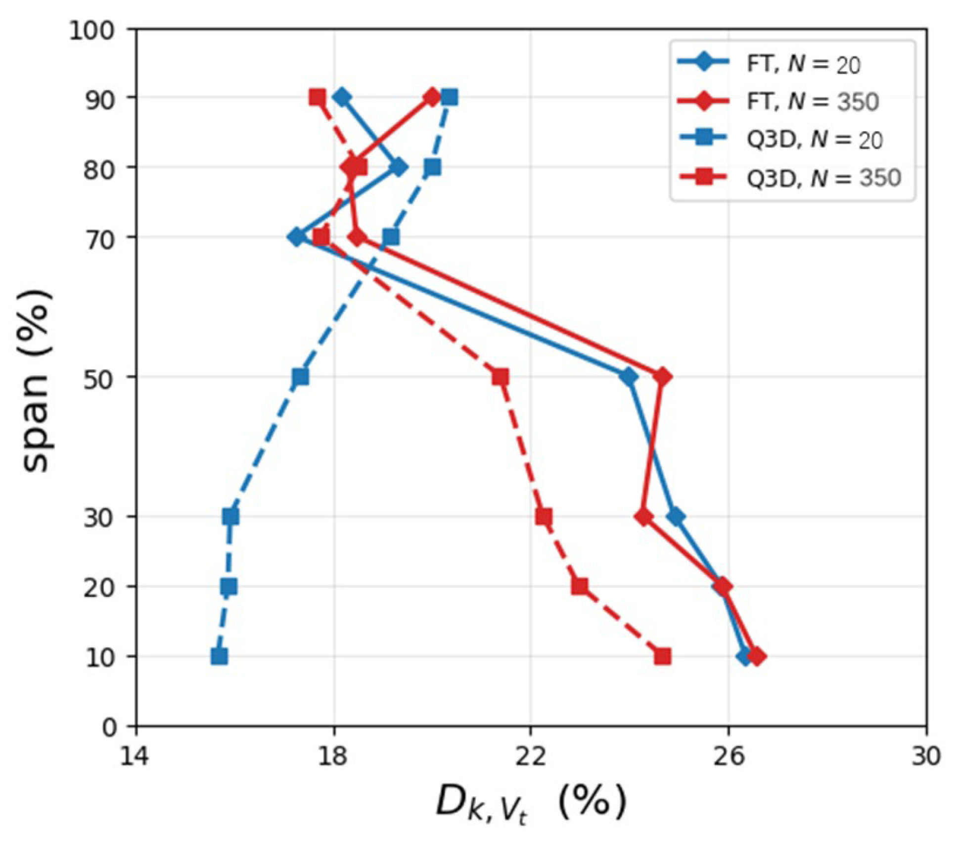
At the same N = 20, the Finetuned backbone without a residual works the hub normally (hub average 25.70%, hub-dominant), whereas the Finetuned Q3D backbone with a residual partner lets go of the hub (hub average only 15.83%, dominance flipped to the tip). After peak normalization, the mean shape difference between the two reaches 0.214 at N = 20 (the Finetuned Q3D curve sits 0.198 lower than Finetuned at the hub end), but drops to 0.034 at N = 350—the two shapes nearly coincide and the flip vanishes.
This controlled comparison rules out the first explanation that the hub information does exist in the N = 20 data and can be extracted by a within-section operator. A division of labor within the joint architecture is the real reason why flip exists. At N = 20, the optimization of Finetuned Q3D assigns the hub correction to the residual module and the backbone retreats toward the tip; at N = 350 the division dissolves and the backbone resumes the hub. The flip is therefore neither a direct image of a 3D physical effect nor a learning failure, but the visible imprint of a labor division whose strength evolves with sample size. The result is shown in Figure 10.
Figure 10.
Backbone adaptation of with and without the residual partner.
The overall scale of the division also evolves with N. Measured against the total correction from the 2D baseline to the true 3D field, the Q3D backbone traverses only about 59% of it at N = 20 and about 81% at N = 350, with the residual supplying the remainder. The more data there is, the more the backbone carries, and the more the residual recedes—consistent with the convergence of the radial shapes.
The dissolution of the division with N implies that the value of the residual module concentrates in the small-sample regime—where the engineering reality of scarce 3D data lies. As data accumulates, the gap between full fine-tuning and the residual architecture narrows. Meanwhile, the controlled comparison shows that pure freezing (Frozen 2D) is not advisable, at least in this case. The backbone must participate in adaptation, and the role of the residual module is to receive the spanwise-coupled component that the backbone structurally cannot express but not to replace the backbone’s adaptation.
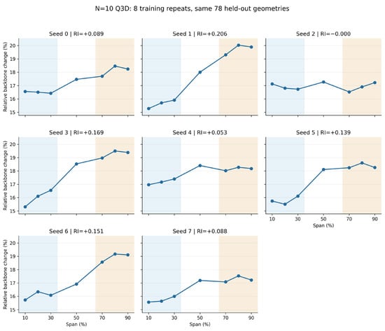
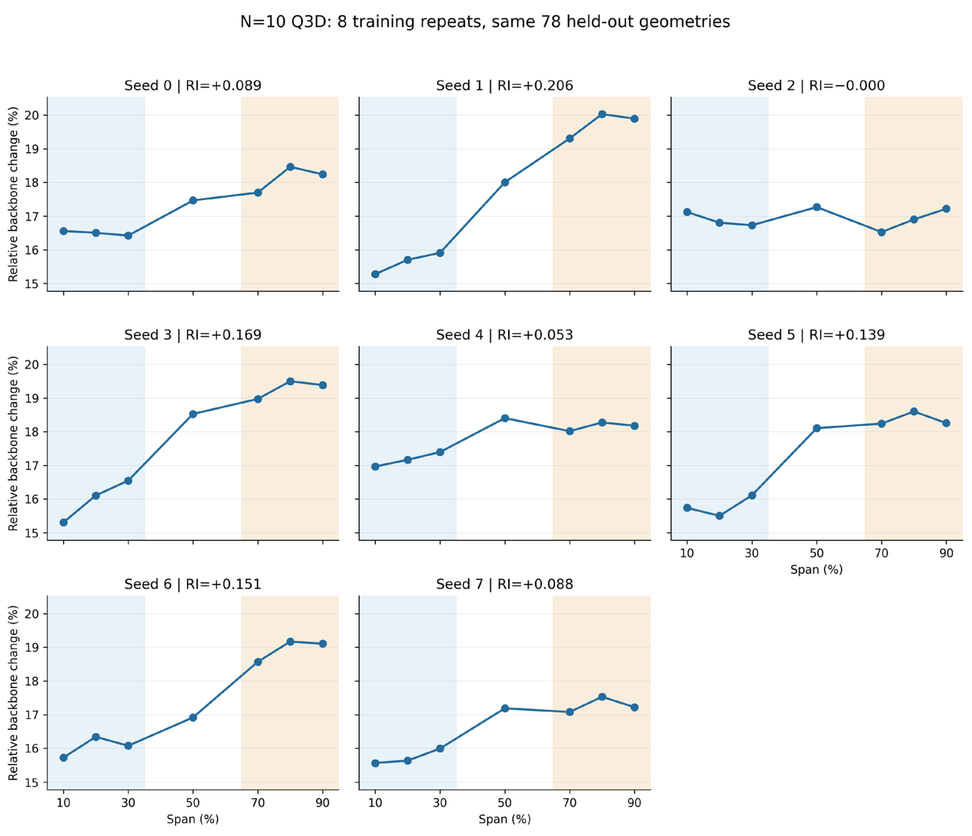
Figure 11 examines whether the relative tip-dominant adaptation observed in the original comparison recurs across training repetitions. Seven of the eight runs exhibit positive relative tip-dominance indices, whereas seed 2 gives a nearly equal mean relative adaptation in the hub and tip regions. The mean RI is 0.1119 ± 0.0670 across the eight runs (mean ± sample standard deviation). The definition of RI is
Figure 11.
Spanwise distributions of relative backbone adaptation for circumferential velocity Vt across eight Q3D training repetitions.
The results show that, except for seed 2, all runs at N = 20 exhibit stronger backbone adaptation at the blade tip than at the hub relative to their respective original baseline magnitudes. This indicates a recurring pattern of adaptation under small-sample conditions. Together with the full-model prediction-error diagnostics, these results support an interpretation of functional allocation rather than overall learning failure. In the original comparison at N = 350, this relative tip-dominant pattern is no longer observed.
3.3. The Architectural Origin of the Division
The division of labor above is not an incidental choice of the optimizer but is predetermined by the architecture’s information pathways. The backbone of Finetuned Q3D inherits the within-section graph of its 2D pretraining. The edge sets of the seven spanwise sections are mutually disconnected, message passing in the backbone is confined within each section, and flow information from one section can never propagate to another inside the backbone. The backbone’s only channel for sensing spanwise position is the nodal input conditions—the per-section Mach number, incidence, and blade-geometry parameters. Consequently, the spanwise variation the backbone can express is strictly limited to a quasi-3D of the weakest kind: a two-dimensional solution per section, driven by that section’s boundary condition which is precisely the assumption of strip theory. Any 3D effect that requires inter-section coupling—spanwise transport, radial equilibrium, the cross-span influence of endwall secondary flows—has no information pathway inside the backbone.
Correspondingly, the residual module is the only component in the joint architecture that owns spanwise edges which are connections between co-located nodes of adjacent sections. The division of labor is thus structurally enforced that the backbone carries the corrections expressible from per-section conditions and corrections requiring spanwise coupling only be carried by the residual module. The flip described in Section 3.2 thereby acquires its mechanism: the 3D correction of hub is dominated by spanwise-coupled effects such as endwall and secondary flows—exactly the structural specialty of the residual module. At small N the optimization assigns it to the residual, and the backbone yields to its expressible tip component. When samples are plentiful, the portion of the hub correction extractable from section conditions grows, the backbone takes over, and the division weakens.
It is worth noting that the Finetuned model still achieves a accuracy, which is better than mean-field baseline, indicating that in this dataset most of the 3D correction can be expressed by the spanwise-varying section conditions, and the part strictly requiring spanwise coupling is a minority.
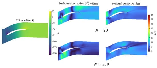
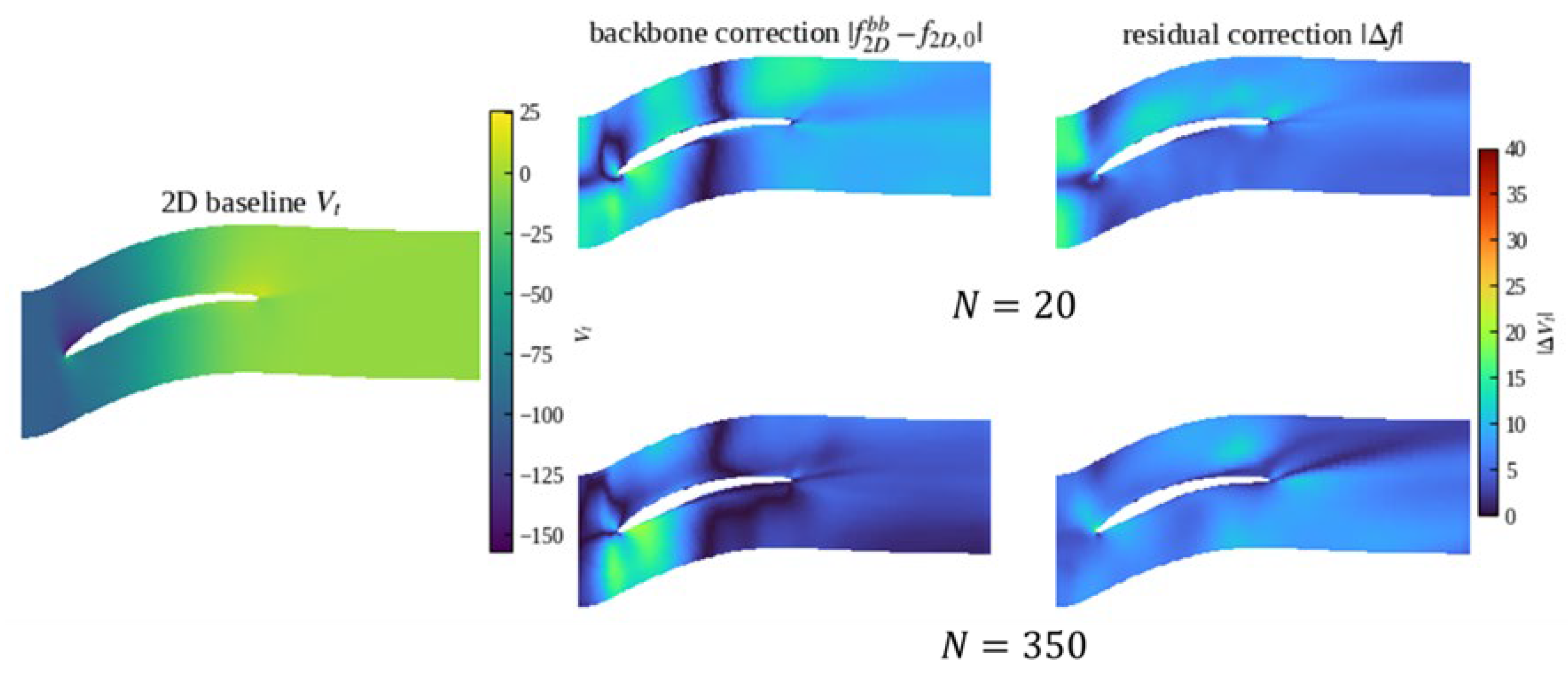
Figure 12 and Figure 13 plot the flow field average correlation distribution in test set of the Finetuned Q3D model’s backbone and residual module with different training samples. Figure 12 shows that near the hub, the 3D effects concentrate at the leading edge and near trailing edge of the suction surface. This is because the camber angle is large and the inflow Mach number is high near the hub, so differences in the hub profile design strongly affect the flow over the rear suction surface. Notably, most of these effects originate from the variation of the flow passage and the per-section conditions that encode the spanwise location, with little dependence on the geometry of adjacent sections—that is, the governing information is available within the section, and in principle lies within the backbone’s reach. At small N the backbone cannot yet pin it down, and the residual module takes over the prediction of the downstream flow field. As training samples accumulate, the mapping becomes calibrated, the backbone fully captures the downstream flow variation, and the residual recedes. Figure 13 shows that, apart from the wake region, the backbone correction is largely insensitive to the sample size, exhibiting only a change in the allocation ratio.
Figure 12.
Backbone vs. residual correlation the at hub section (10% span).
Figure 13.
Backbone vs. residual correlation the at tip section (90% span).
To assess the sensitivity of the results to restricting the backbone to in-section connections, we conducted experiments incorporating 0%, 5%, and 20% of all available adjacent-section connections into the backbone. As shown in Table 8, adding these connections increased message-passing computation without changing the parameter count, yielded only modest accuracy improvements, and did not qualitatively alter the reversal pattern observed for . However, introducing spanwise edges into the backbone changes the graph structure used during two-dimensional pretraining and introduces an additional pathway for spanwise adaptation. Therefore, the proposed architecture retains a purely in-section backbone and assigns all explicit spanwise connections to the residual branch, preserving the pretrained graph structure while introducing spanwise communication through a separate module.
Table 8.
Test NRMSE for four flow variables with different fractions of spanwise connections incorporated into the backbone.
3.4. The Quantitative Analysis of Labor Division and Data
Section 3.2 and Section 3.3 established the existence and the architectural origin of the division of labor, while this section answers what determines its allocation ratio. The central proposition is: the harder a 3D correction is to regress from 2D conditions, the more it relies on the residual module.
To measure the information that can be learned within section geometry, inlet condition, and independent from the architecture of neural network, a ridge-regression probe is proposed. The inputs are the section’s condition parameters plus nodal position, the target is the true 3D correction there (CFD minus the 2D prediction), and the score is the cross-sample on the test split. This quantity is a pure data property, independent of every GNN in this work. The division ratio is measured directly from explicit decomposition and the residual share is (defined in Equation (4)).
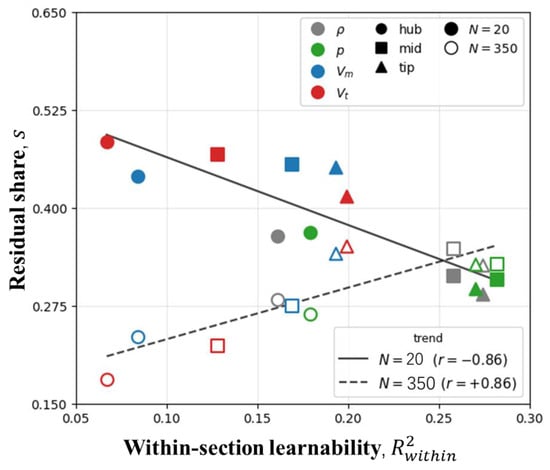
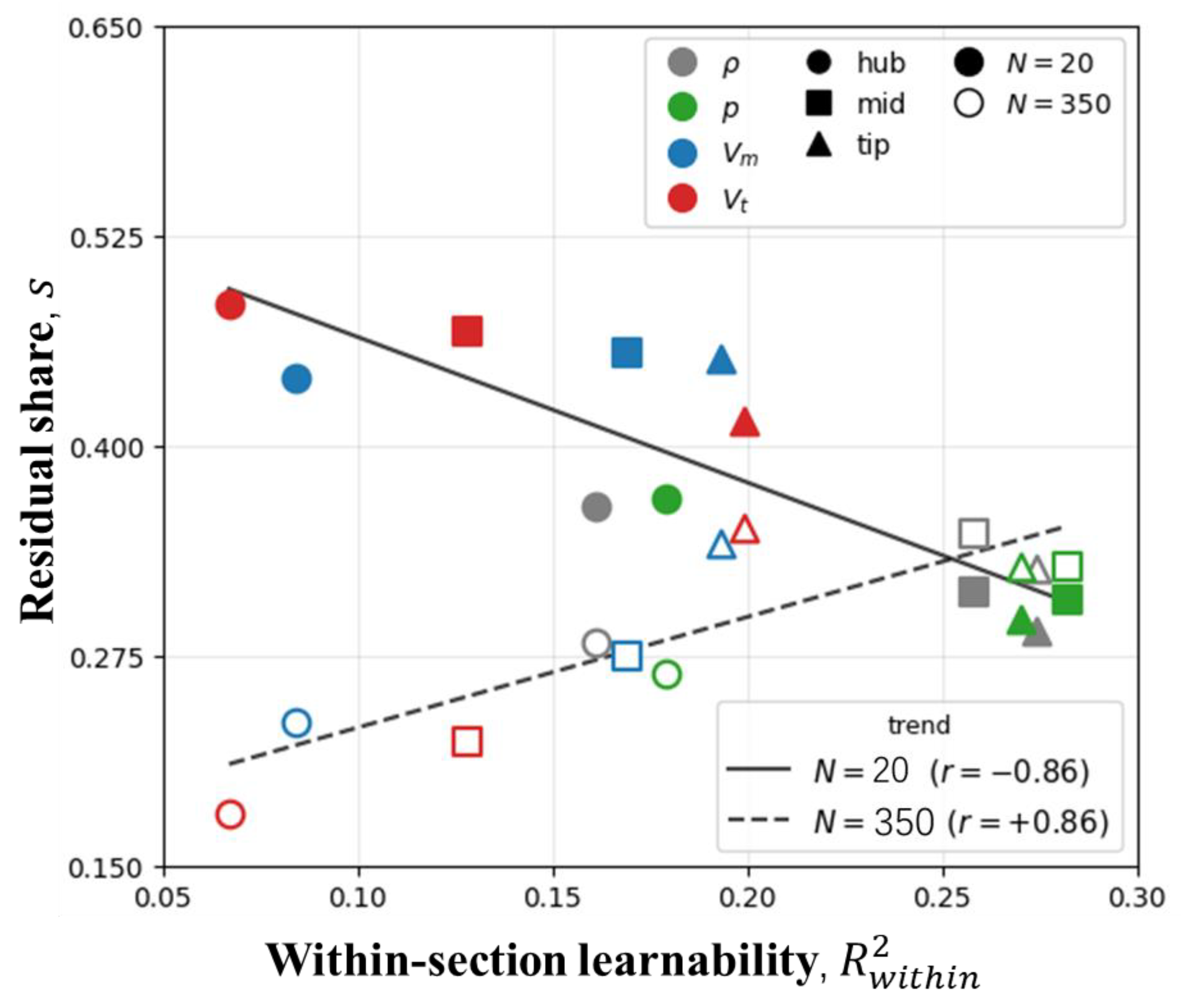
Computing both quantities for all combinations of four aerodynamic variables × three spanwise zones (hub/mid/tip) × two sample sizes (N = 20 and N = 350), yields the learnability–division scatter. The results are shown in Figure 14. The division of labor is governed by data learnability at small N and dissolves with data, residual share versus , with the correlation reversing from −0.86 to +0.86.
Figure 14.
Residual share of the division of labor versus within-section learnability of the 3D correction.
The result exhibits a clear twofold regularity:
(i) N = 20: Learnability drives the division. The residual share is strongly anti-correlated with (r = −0.86). The harder a quantity is to regress within-section, the more the residual carries. The ordering across variables is fully consistent— has the lowest within-section learnability (mean 0.131) and the highest residual share (0.455); (0.149/0.449); and have the highest learnability and the lowest residual shares (0.231/0.322, 0.244/0.324). The spanwise level also agrees in direction while hub is the least learnable of all combinations and carries the highest residual share among the zones (0.484).
(ii) N = 350: The division dissolves with data. The correlation flips sign to +0.86, and the residual share drops across the board (e.g., hub falls from 0.484 to 0.181). The interpretation: once samples are plentiful, the former learnability gap is filled by data, the backbone takes over the hard regions, the residual recedes to supplying high-frequency detail, and the mechanism “learnability gap drives the division” ceases to operate. The sign flip of the correlation is precisely the signature of that mechanism being dissolved by data.
The division of labor between backbone and residual module in the transfer architecture and its regularities are the central findings of this study. The division is enforced by the architecture’s information pathways (within-section vs. spanwise), its allocation ratio is determined by the within-section learnability of the data, and it dissolves as samples accumulate. This picture elevates the widely used “pretrained backbone + residual adapter” transfer paradigm from an empirical design to a diagnosable, predictable mechanism. For a new physical quantity or a new flow region, its within-section learnability predicts whether the backbone or the adapter will carry it, and the size of dataset needed.
4. Conclusions
This paper studied cross-dimensional transfer for compressor flow-field prediction on a stator using Q3D-GTN: a quasi-3D graph of seven blade-to-blade sections stacked with spanwise edges, on which a 2D-pretrained in-section backbone supplies the baseline and an identity-initialized spanwise residual module learns the correction, . Beyond showing that the method works, this study explored the transfer mechanism and traced it to a property of the data.
- Transfer learning moves the model from unusable to usable. At N = 20, the ablation experiment shows that replacing a node-local residual with a spanwise residual reduces mean NRMSE across the four predicted quantities, supporting a benefit from spanwise communication. Finetuned Q3D achieves lower errors than Finetuned, Frozen-2D, and Scratch for all four quantities in all three paired repetitions. For tangential velocity, their mean NRMSE values are 0.36, 0.47, 0.56, and 0.83, respectively. Since the two differ only in the residual module, Finetuned Q3D’s consistent margin at every budget is attributable to the spanwise coupling it captures. Freezing the backbone is inadvisable since the residual alone cannot bridge the full 2D-to-3D gap.
- Backbone and residual divide the task in a structured way. We conducted a 3D-to-2D back-reaction analysis of finetuned model with or without residual module. The controlled comparison showed that at small N the joint architecture assigns corrections requiring inter-section coupling to the residual, while the backbone—message passing confined within sections—carries what per-section conditions can express. The radial dominance flip in the backbone’s adaptation is the imprint of this division, the division is strongest at N = 20 and dissolves by N = 350.
- The allocation is governed by a measurable data property. A network-independent Ridge regression probe of within-section learnability shows the residual share strongly anti-correlated with learnability at N = 20. At N = 350, the correlation reverses and shares drop—the learnability-driven division dissolves once data fill the gap. Practically, a lightweight pre-training probe predicts which component will carry a quantity and when the residual’s value fades.
Together, these results elevate the “pretrained backbone + adapter” recipe into a diagnosable, predictable mechanism: information pathways dictate what kind of correction each component can carry; data learnability dictates how much; the sample budget dictates how long the division persists. These results offer practical guidance for transfer-learning-based modeling and database planning in aero-engine fluid dynamics.
Author Contributions
Conceptualization, Y.F.; methodology, Y.F.; validation, Y.F., T.P., and W.Y.; formal analysis, Y.F.; investigation, Y.F.; resources, Y.F.; data curation, Y.F.; writing—original draft preparation, Y.F.; writing—review and editing, T.P. and W.Y.; visualization, Y.F.; supervision, T.P. and W.Y.; project administration, T.P.; funding acquisition, T.P. All authors have read and agreed to the published version of the manuscript.
Funding
The authors acknowledge the support of Taihang National Laboratory (No. B7013) and the National Natural Science Foundation of China (No. 52322603).
Data Availability Statement
The data presented in this study are available on request from the corresponding author.
Conflicts of Interest
The authors declare no conflict of interest.
Abbreviations
The following abbreviations are used in this manuscript:
| Q3D-GTN | Quasi-3D Graph Decomposition Transfer Networks |
| B2B | Blade-to-blade |
| CFD | Computational Fluid Dynamics |
| GNN | Graph Neural Network |
| GCN | Graph Convolutional Network |
| MLP | Multilayer Perceptron |
| SST | Shear Stress Transport |
| NRMSE | Normalized Root Mean Square Error |
| relL2 | Relative L2 Error |
References
- Aungier, R.H. Axial-Flow Compressors; ASME Press: New York, NY, USA, 2003. [Google Scholar]
- Cumpsty, N.A.; Greitzer, E.M. Ideas and Methods of Turbomachinery Aerodynamics: A Historical View. J. Propuls. Power 2004, 20, 15–26. [Google Scholar] [CrossRef] [Scilit]
- Wu, L.; Kim, J.W.; Wilson, A.G.; Shahpar, S. Automatic Design Optimization of a Transonic Compressor Rotor for Improving Aeroacoustic and Aerodynamic Performance. J. Turbomach. 2022, 144, 081016. [Google Scholar] [CrossRef] [Scilit]
- Pan, T.; Li, T.; Yan, Z.; Li, Q. Turbulence-induced disturbances and their evolution to stall onset in a compressor cascade using large eddy simulation. Chin. J. Aeronaut. 2026, 39, 103491. [Google Scholar] [CrossRef] [Scilit]
- Pan, T.; Li, Q.; Li, Z.; Gong, Y. Effects of radial loading distribution on partial-surge-initiated instability in a transonic axial flow compressor. J. Turbomach. 2017, 139, 101010. [Google Scholar] [CrossRef] [Scilit]
- Pfaff, T.; Fortunato, M.; Sanchez-Gonzalez, A.; Battaglia, P.W. Learning Mesh-Based Simulation with Graph Networks. arXiv 2021, arXiv:2010.03409. [Google Scholar]
- Li, J.; Liu, T.; Wang, Y.; Xie, Y. Integrated graph deep learning framework for flow field reconstruction and performance prediction of turbomachinery. Energy 2022, 254, 124440. [Google Scholar] [CrossRef] [Scilit]
- Li, J.; Li, Y.; Liu, T.; Zhang, D.; Xie, Y. Multi-fidelity graph neural network for flow field data fusion of turbomachinery. Energy 2023, 285, 129405. [Google Scholar] [CrossRef] [Scilit]
- Li, J.; Liu, T.; Zhu, G.; Li, Y.; Xie, Y. Uncertainty quantification and aerodynamic robust optimization of turbomachinery based on graph learning methods. Energy 2023, 273, 127289. [Google Scholar] [CrossRef] [Scilit]
- Strönisch, S.; Sander, M.; Meyer, M.; Knüpfer, A. Prediction of steady and unsteady flow quantities using Multiscale Graph Neural Networks. J. Turbomach. 2025, 147, 071015. [Google Scholar] [CrossRef] [Scilit]
- Blechschmidt, D.; Mimic, D. Predicting Time-Averaged Unsteady Flows in Turbomachinery via Graph Neural Networks. J. Turbomach. 2026, 148, 011003. [Google Scholar] [CrossRef] [Scilit]
- Li, Z.; Montomoli, F.; Sharma, S. Investigation of compressor cascade flow using physics-informed neural networks with adaptive learning strategy. AIAA J. 2024, 62, 1400–1410. [Google Scholar] [CrossRef] [Scilit]
- Feng, Y.; Yuan, W.; Song, X.; Yan, Z.; Pan, T. Prediction of subsonic cascade flow fields by physics-informed graph neural networks with unbalanced data. Aerosp. Sci. Technol. 2025, 162, 110173. [Google Scholar] [CrossRef] [Scilit]
- Subel, A.; Guan, Y.; Chattopadhyay, A.; Hassanzadeh, P. Explaining the physics of transfer learning in data-driven turbulence modeling. PNAS Nexus 2023, 2, gad015. [Google Scholar] [CrossRef] [Scilit] [PubMed]
- Liu, Y.; Liu, W.; Yan, X.; Guo, S.; Zhang, C.-A. Adaptive transfer learning for PINN. J. Comput. Phys. 2023, 490, 112291. [Google Scholar] [CrossRef] [Scilit]
- Wang, Z.; Liu, X.; Yu, J.; Wu, H.; Lyu, H. A general deep transfer learning framework for predicting the flow field of airfoils with small data. Comput. Fluids 2023, 251, 105738. [Google Scholar] [CrossRef] [Scilit]
- Wu, M.-Y.; He, X.-J.; Sun, X.-H.; Tong, T.-S.; Chen, Z.-H.; Zheng, C. Efficient aerodynamic shape optimization using transfer learning based multi-fidelity deep neural network. Phys. Fluids 2024, 36, 116109. [Google Scholar] [CrossRef] [Scilit]
- Li, R.; Zhang, Y.; Chen, H. Transfer Learning from Two-Dimensional Supercritical Airfoils to Three-Dimensional Tran-sonic Swept Wings. Chin. J. Aeronaut. 2023, 36, 96–110. [Google Scholar] [CrossRef] [Scilit]
- Yang, Y.; Li, R.; Zhang, Y.; Chen, H. Transferable Machine Learning Model for the Aerodynamic Prediction of Swept Wings. Phys. Fluids 2024, 36, 076105. [Google Scholar] [CrossRef] [Scilit]
- Li, Q.; Yan, J.; Pan, T.; Li, T.; Su, G.; Tao, Z. Critical loading identification of compressor stall and vortex criterion in rotational frame. AIAA J. 2025, 63, 4054–4067. [Google Scholar] [CrossRef] [Scilit]
- Liu, Z.; Li, T.; Zheng, M.; Li, Q.; Pan, T. Feedback-driven nonlinear amplification of leading-edge spillage and its role in stall triggering in a low-speed compressor. Aerosp. Sci. Technol. 2026, 176, 112627. [Google Scholar] [CrossRef] [Scilit]

Disclaimer/Publisher’s Note: The statements, opinions and data contained in all publications are solely those of the individual author(s) and contributor(s) and not of MDPI and/or the editor(s). MDPI and/or the editor(s) disclaim responsibility for any injury to people or property resulting from any ideas, methods, instructions or products referred to in the content. |
© 2026 by the authors. Licensee MDPI, Basel, Switzerland. This article is an open access article distributed under the terms and conditions of the Creative Commons Attribution (CC BY) license.