


Highlights
What are the main findings?
- For eight multicopter source fields, directional spectra show redistribution that depends on the flight regime, and this occurs within one shared frequency range.
- Angular, 960-observer and interior-state tests serve to quantify means and tails, while outdoor measurements reveal a considerable mismatch in absolute levels.
What are the implications of the main findings?
- Directional spectra retain the information that scalar source levels discard; for data of this kind, RBF constitutes a reconstruction candidate associated with lower error.
- Comparisons at new receiver positions and outdoors distinguish reconstruction quality from the material discrepancy in physical prediction.
Abstract
Directional spectra preserve source information for trajectory-based noise models, but low reconstruction error does not establish physical source accuracy. We present a JSON database for eight X500 multicopter states, each with 266 receiver directions at approximately 1 m. Our comparison uses 25 complete, one-third-octave bands from 50 Hz to 12.5 kHz. Repeated grouped directional holdouts yield mean-square-pressure (MSP) OASPL MAE of 0.3–0.8 dB, P95 up to 3.3 dB, maximum OASPL error of 9.1 dB, and maximum individual-band error of 26.8 dB. Expanding the RBF candidates, selecting parameters on training data, and applying numerical guards reduces MAE to 0.09–0.44 dB. Full-density transfer to 960 independently located, ground-directed receivers from the same climb-2 CFD source gives MSP OASPL MAE/P95/maximum of 1.11/2.91/3.98 dB and restricted A-weighted MAE of 0.57 dB. MSP remains the default for ground-directed transfer. Withheld interior speed states give OASPL MAE of 0.42–1.18 dB. Outdoor hover observations at altitudes of 10 and 20 m exceed propagated database levels by mean differences of 15.3–19.0 dB across recorder sequences. This discrepancy does not establish absolute community-noise accuracy. Temporal record sensitivity, coordinate correction, triangle quality, integrated-field consistency, and measured query costs define the supported reconstruction use and remaining source/propagation validation requirements.
1. Introduction
Source spectra that preserve both radiation directionality and operating state are needed to predict urban air mobility (UAM) noise. The receiver’s distance and orientation with respect to the source change as aircraft move through space. If these variables are retained, a database can provide trajectory-model inputs without fresh source-data collection for every query. The ultimate aim is a cost-effective source-data resource, yet this work assesses its representation and reconstruction capacities. A method for computing airplane noise near airports is set out in SAE AIR1845A [1]. In the Aviation Environmental Design Tool (AEDT) [2,3], noise–power–distance (NPD) datasets link UAM source calculations to community-noise evaluations. For rotorcraft assessment, directional information is retained by noise hemispheres [4], while the acquisition conditions required to interpret these fields are defined by a NASA flight-test protocol [5]. Consequently, data must be accompanied by propagation conventions, receiver geometry, and source state. Vehicle and component acoustics have been examined in earlier multicopter research. Small rotary-wing components are characterised and forecast by Zawodny et al. [6], whereas quadcopter performance and acoustics under static thrust are studied by Intaratep et al. [7]. Directivity and spectral emission are reviewed by Schäffer et al. within the wider drone-noise literature [8]. Receiver signals are synthesised by Heutschi et al. from lab-based drone recordings, with adjustments for operational and propagation factors [9]. Rather than assigning a single level per source state, these studies support keeping directional spectra.
To evaluate community exposure, stationary unweighted OASPL alone is insufficient. Aircraft exposure should be kept below 45 dB and 40 dB , according to the WHO 2018 guidelines. is an annual day–evening–night exposure indicator and is not the same as daytime source levels [10]. Drone-specific legal certification limits are not established by these health recommendations. Event , sound exposure level (SEL), operation counts, route geometry, and time of day link source spectra to exposure. In addition, UAM annoyance is influenced by loudness, sharpness, roughness, fluctuation strength, and tonality [11]. Band-based A weighting is possible with one-third-octave data, but narrowband tonality or phase-dependent temporal sound quality cannot be recovered from them. Inputs for such assessments can be provided by a directional database, yet acceptance or regulatory compliance is not determined by it.
For a given operation, an NPD computation begins with source spectra that depend on state. Propagation together with trajectory geometry subsequently yields ; SEL and are then derived from it at reference distances, indexed by a parameter of operating power. The airport-noise model thereupon applies its procedures for events and exposure [1,2,12]. A short stationary spectrum captured at 1 m is not, by itself, an AEDT NPD table. Separate demonstrations employing the NASA hemisphere protocol, along with small-rotor experiments, highlight how necessary it is to govern near-field and far-field behaviour and the conditions of operation [5,6,7].
Hover spectra have been confirmed by recent UAV propeller investigations, which also examine options for permeable FW–H surfaces [13]. Radial decay and directivity are evaluated through rotor-rig measurements spanning isolated, installed, and four-rotor arrangements [14]. Why observer radius and source configuration each demand separate control is shown by both studies. Evolving national drone policy, engagement with stakeholders, and proportionate noise management for emerging aircraft are covered by current UK CAA guidance [15]. Decisions of this practical kind depend on credible receiver exposure rather than on numerical reconstruction error alone.
A well-established numerical method is spherical interpolation. Work in acoustics on head-related transfer functions (HRTF) indicates that reconstruction on sparse irregular grids is influenced by regularisation and by spherical-harmonic (SH) order [16]. These complex transfer functions are unlike the scalar band levels adopted here, yet SH is still a pertinent comparator for directional reconstruction. As an alternative, a radial-basis function (RBF) interpolator offers a further representation for scattered data. Mean-square-pressure interpolation is therefore treated as a methodological option under assessment, not put forward as new interpolation theory. Drawing on the authors’ corridor frameworks and methods of source acquisition [17,18], eight multicopter source states are arranged in this study into a directional spectral database intended for prediction-model development. The contributions comprise an explicit source-data contract covering coordinate conventions and frequency support, an audit of the receiver records supplied, and a matched comparison of reconstruction by MSP, in the dB domain, by SH, and by RBF. Angular reconstruction, full-density layout transfer, interior-state interpolation, and outdoor physical comparison are each distinguished in this assessment. Practical choices are weighed through cost diagnostics and numerical metrics, though no environmental certification or CFD convergence is established. Table 1 sets these contributions against related acoustic work.
Table 1.
Position of the present database study within related acoustic work.
2. Materials and Methods
2.1. Source Database and Acquisition
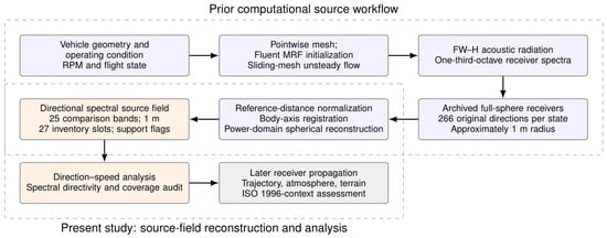
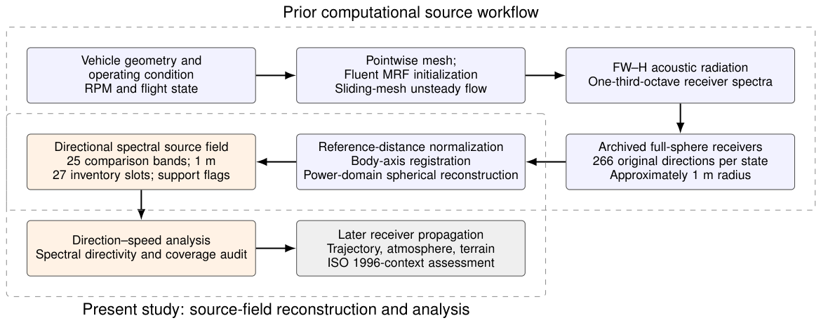
A compact, four-rotor testbed, the X500 is fitted with two-bladed, 10-inch propellers. The platform was selected because computational and outdoor acoustic data already exist for it. This availability makes evaluation of the database architecture manageable; nevertheless, the platform is not representative of a full-scale, passenger eVTOL. The eight states supplied consist of hover, climb at 1–3 m/s, and cruise at 2–8 m/s. In acquiring sources, pointwise Fluent MRF initialisation is combined with sliding-mesh flow and FW–H receiver calculations [17,19,20]. The separation between source acquisition, database construction, and receiver application is illustrated in Figure 1.
Figure 1.
Source acquisition, database construction and subsequent receiver propagation. Source CFD accuracy and reconstruction accuracy are separate assessments.
For all eight states, a single k– shear-stress-transport model is employed, together with second-order upwind schemes for momentum and turbulence, second-order pressure, and coupled pressure–velocity solutions. Rotational inputs and receiver sampling intervals are listed in Table 2. The rotational parameters of cruise-4 and cruise-6 come from the retained PWM-to-RPM operating record. By comparing these with the corresponding hover, cruise-2, and cruise-8 records, the motor numbering was mapped onto the CFD zone order. The documented grids hold approximately 8.918 million cells for hover, cruise-2, and cruise-8; climb cases, by contrast, involve 8.716 million cells. The RPM inputs are assigned to the rotating fluid-cell zones 12, 16, 20, and 24, whereas the corresponding rotor-wall boundary zones 15, 19, 23, and 27, respectively, define the FW–H acoustic surfaces. Alternating rotation axes apply to the fluid zones, whose rotor centres lie near m. Given a rotor diameter of 0.254 m, the bounding source radius is roughly 0.40 m, and the bounding diameter 0.80 m. These inputs characterise the source fields used in the database assessment, but they do not establish mesh-convergence accuracy.
Table 2.
Operating inputs for the eight acoustic source states. Rotor RPM order follows rotating fluid-cell zones 12, 16, 20 and 24. Sampling intervals are measured from receiver histories, not inferred solver time steps.
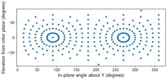
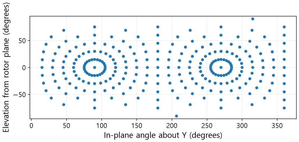
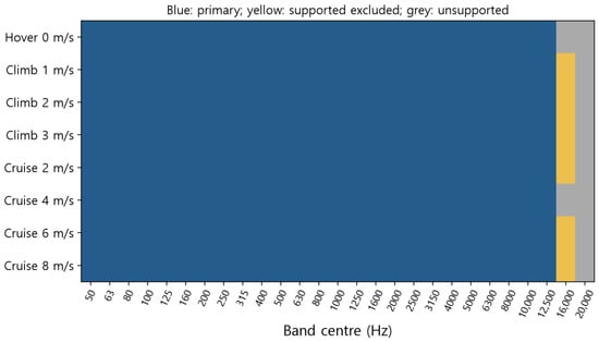
Every field contains 266 distinct receiver directions, all positioned at m. Within the common comparison set there are 25 finite complete bands, whose preferred centre frequencies span 50 Hz to 12.5 kHz [21]. Support at the complete-band level depends on . Neither the finite 20 kHz entries nor a query grid with one-degree spacing establishes temporal or angular resolution. Record support is outlined in Table 3, the acquisition directions are shown in Figure 2, and the resulting complete-band support is summarised in Figure 3.
Table 3.
Temporal-support audit over 266 histories per state. The 16 kHz and 20 kHz upper edges are 18.0 and 22.4 kHz, respectively. No state supports the entire 20 kHz band.
Figure 2.
The 266 acquisition directions. Elevation is measured from the physical rotor plane XZ; +Y is upward.
Figure 3.
Complete-band support. Blue denotes the primary 50 Hz–12.5 kHz range; yellow denotes supported excluded bands; grey denotes unsupported complete bands.
2.2. Coordinates, Reconstruction and Receiver Propagation
With a source located at and a receiver at ,
The direction running from source to receiver is given by . Under the rotor settings actually employed, the simulator’s vertical axis is Y. The registration stored numerically as keeps Y fixed while mirroring Z. Because its determinant is , this registration is not an attitude rotation. Signed X and Z represent the in-plane axes, and neither carries a physical port or starboard designation. The coordinates adopted for plotting are and , together with . The earlier interpretation, under which the XY section was taken to be horizontal, has been superseded by the corrected rotor-plane plots. Angular holdout errors are unchanged when a common orthogonal registration is applied.
In the MSP reconstruction, the unit vectors are triangulated by means of their convex hull, with barycentric weights that are non-negative and normalised:
scales in proportion to the mean-square pressure, so pressure waveforms need not be interpolated. For scalar levels, the energy mean of the training spectra across all directions is used, while nearest lookup picks whichever training spectrum has the least angular separation. Directivity is disregarded by the former baseline and local continuity by the latter. State, bands, signed coordinates, reference distance, valid masks and provenance are all stored by the JSON schema 5. JSON null denotes any nonfinite value.
A positive propagation loss must be subtracted when receiver levels are estimated:
where denotes the atmospheric absorption coefficient given in ISO 9613-1 [22]. Primary layout and experimental comparisons make use of . Absorption is included in a sensitivity analysis under conditions explicitly assumed to be 20 °C, 50% relative humidity and 101.325 kPa. No fitting to observations was performed for ground interaction, shielding or meteorological refraction. Consequently, only the current source-plus-free-field chain is assessed by the open-stadium comparison, and no validated urban propagation model is established.
Only is covered by the A-weighted result; it does not constitute a full-band environmental . For far-field transfer, is required, together with for reactive components and a small aperture phase-curvature term on the order of . These amount to separate conditions [20]. With m and m/s, a radius of 1 m corresponds to , while occurs at 50 Hz. At 12.5 kHz and 1 m, the aperture phase term is approximately 18 rad. Hence spherical spreading over the whole band cannot be validated by any single cutoff.
2.3. Angular Holdouts and Numerical Diagnostics
Five grouped, five-fold partitions are controlled by seeds 41, 73, 101, 151, and 211. Before grouping and splitting, unit directions are rounded to nine decimal places. In each outer model, training uses roughly 80% of the 266 directions, and every remaining direction is assessed once per repetition. Accordingly, the 1330 predictions per state draw on the same 266 source observations. For direct dB interpolation, triangles from MSP are used. Real spherical harmonics (SH) are applied with degrees 3, 5, and 7, and with a ridge coefficient set to 0.001 times the mean diagonal of the normal matrix. Within every outer training set, candidate selection is governed by OASPL MAE through three inner folds. Final evaluation alone uses outer truth. Training-only nested selection is therefore established by this protocol.
In the original RBF comparison, a thin-plate spline was used with 32 neighbours and smoothing parameters of 0, 0.01, or 0.1. The expanded search brings together thin-plate-spline, cubic, and linear kernels, together with 16/32/64 neighbours and smoothing values of 0/0.01/0.1/1, which gives 36 candidates in SciPy 1.13.1, [23]. For degree-one local polynomial systems, the smallest-to-largest singular-value ratio must be at least . A prediction is rejected when it is nonfinite, or when any band falls outside the training range, extended by 40 dB. Then, according to inner-score order, the next admissible candidate is selected. Geometry and training spectra underpin this safeguard, so outer truth is not consulted. Although it reduces the instability observed in local, zero-smoothing fits, no conservation is implied.
Error summaries report MAE, RMSE, nearest-rank P95, maximum absolute OASPL error and separate individual-band errors. For the original conditional intervals, absolute errors are first averaged across repetitions; 266 direction clusters are then resampled 2000 times (seed: 20261004). These intervals do not quantify source CFD uncertainty. Triangle diagnostics compute great-circle interior angles in each held-out triangulation and their Spearman correlation with error. Integrated-field consistency compares source spherical-Voronoi quadrature with a 60-point Gauss–Legendre method using 120-azimuth quadrature. This integrates mean-square-pressure surrogates over solid angle, but does not measure sound power at 1 m.
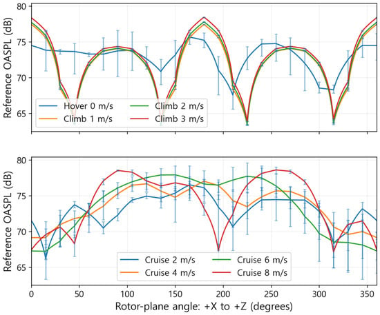
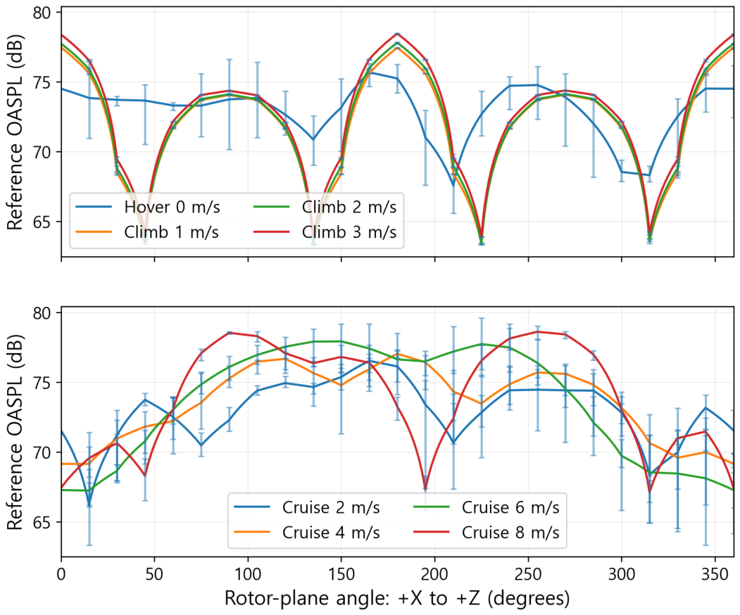
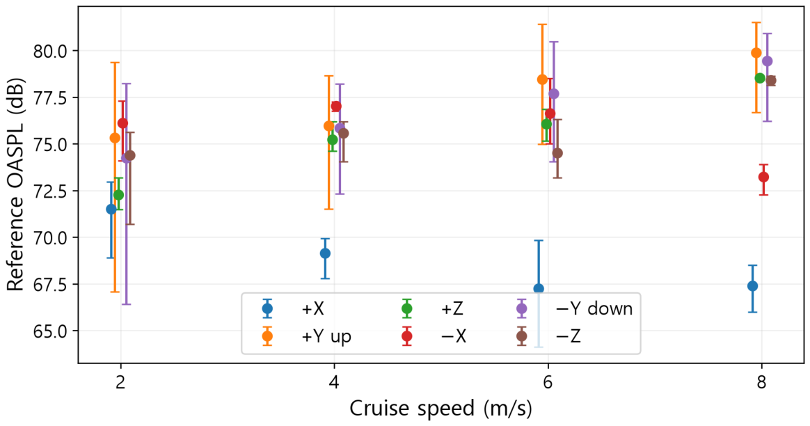
The temporal sensitivity analysis takes in the full pressure record together with three contiguous blocks of equal length. After the mean has been removed, rectangular-window FFTs are zero-padded up to the next power of two and integrated from 44.5 Hz to 14.0 kHz, which forms the continuous outer edges of . No physical resolution is introduced by zero padding. In Figure 4 and Figure 5, the error bars span both the archived centre levels and the recomputed full/block levels, evaluated at the original receiver directions. Ranges of sensitivity for finite records are what such bars represent; they should not be treated as independent standard deviations or as confidence intervals.
Figure 4.
OASPL in the physical rotor plane XZ at 1 m. Angle runs from +X towards registered +Z. Bars at original receivers span archived and full/three-block reanalyses; they are finite-record sensitivity ranges.
Figure 5.
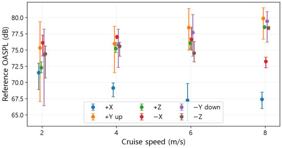
Cruise OASPL at the six signed axes. Bars give the finite-record sensitivity ranges defined in Methods; markers are horizontally offset for legibility.
Model setup, the median over five warm batches of 1000 queries, and the median over 50 single-direction calls are distinguished by the query-cost measurements. All 266 source points and identical 25 bands are used by both approaches on a Windows x64 workstation equipped with an Intel Core i7-14700 processor. Threads in the numerical library are capped at one. Storage for owned NumPy arrays is reported apart from peak process memory. Model calls following candidate selection are included in the timings, whereas additional guard overhead is not. New query directions do not require retraining. If source directions are added, however, the geometry or RBF neighbour structures must be rebuilt, and, where relevant, RBF parameters must be re-selected.
2.4. Full-Density Layout Transfer, Interior States and Outdoor Comparison
For radii of 2.50–50.99 m, the full climb-2 source field yields 960 direct spectra that come from the same CFD source. The negative-Y geometry, intended for downward, ground-directed use, consists of 24 transverse angles, five radii, and eight axial layers; it is neither a uniform rectangular grid nor one ground plane. The reported errors combine angular reconstruction with the imposed radial law. A fixed thin-plate-spline RBF takes 32 neighbours and a smoothing value of 0.01, and is not tuned to these external observations; such settings differ from those of the expanded, nested RBF search. A second full-density RBF applies the cubic/32-neighbour/zero-smoothing option, chosen by three-fold validation using only 266 source samples. When this is applied to the same external set, subject to the stated guards, no selection against external truth is involved.
One at a time, climb 2 m/s, cruise 4 m/s, and cruise 6 m/s are each withheld completely, which allows conditions absent from a source lookup to be tested. Equal linear-energy mixtures of the two same-mode states that bracket each withheld speed provide the predicted spectra, evaluated at the 266 directions belonging to that withheld state. No spectrum from the target state is included in the model. Thus, the procedure tests interpolation at an interior speed, rather than extrapolation to new RPM, a new attitude, or conditions outside the range.
The same X500 platform and rotors were used for outdoor hover observations at the main stadium of Konkuk University. Five microphone locations are covered by each of the two recorder sequences. In the outdoor campaign, an unobstructed layout was used, with Dayton Audio EMM-6 microphones, two ZOOM F6 recorders, and an acoustic calibrator for every experiment. Source altitudes are 10, 20, 30, 40, 60, 70 and 100 m. Along an axis, horizontal offsets are 2 or 5 m, whereas diagonal sites have 5 m offsets on both horizontal axes. The documented microphone height of 1.5 m is used in the reference calculation. Height sensitivity spans 1.2–1.5 m, and heading sensitivity spans 24 headings at 15-degree intervals, so that departures from the prescribed height and heading uncertainty can be assessed. At altitude H, the source-relative query is , and the propagation range is set by its norm. Archived equivalent A-weighted levels are compared with the restricted-band prediction, without fitting an amplitude correction or subtracting noncontemporaneous background. According to the campaign records, background limitations arise beyond approximately 30 m. Those observations are still plotted, but they are not treated as accurate, source-isolated high-altitude validation. Equivalent levels are not the same as the separately reported Fast Max [24,25].
3. Results
3.1. Frequency Support and Corrected Directional Fields
Finite predictions are obtained at every query direction for all 25 selected bands. Such 100% coverage constitutes an array-support finding, and it carries no implication regarding physical accuracy. Inventory entries at high frequency that lack support are left out of Figure 3.
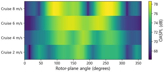
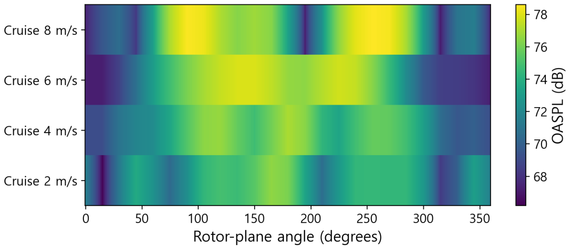
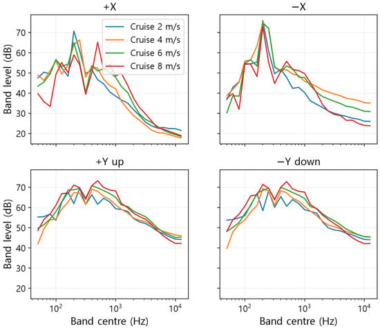
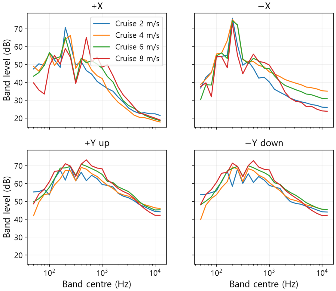
The confirmed vertical axis changes the physical interpretation of earlier signed-section plots. Whereas Figure 4 shows the rotor plane XZ, Figure 5 indicates upward +Y and downward . Common-band levels and numerical database tuples remain unchanged. Temporal bars imply that variability in finite records necessitates separate evaluation from angular reconstruction. Table 4 summarises cruise OASPL at the six signed-axis directions in the common band; Figure 6 and Figure 7 show rotor-plane levels and signed-axis spectra, respectively.
Table 4.
Signed-axis cruise reference OASPL over 50 Hz–12.5 kHz (dB). Y is vertical and X/Z lie in the rotor plane.
Figure 6.
Rotor-plane cruise OASPL at the four sampled speeds. Display density is a query density rather than independent acoustic resolution.
Figure 7.
Cruise spectra in the signed streamwise and vertical directions. All curves use the same 25 supported bands.
3.2. Held-Out Directional Reconstruction
Across the eight conditions, finite predictions were obtained for all 25 comparison bands at each held-out direction. Table 5 lists the errors with respect to the original, computed receiver spectra. In all states, the overall-level MAE, which ranges from 0.3 to 0.8 dB, is below both the scalar and nearest-direction references. For the interpolator, the absolute overall-level error at the 95th percentile falls between 0.9 and 3.3 dB, although the largest individual error, 9.1 dB, arises during climb at 3 m/s. Consequently, small reconstruction errors are not assured by complete coverage alone.
Table 5.
Held-out overall-level reconstruction over 25 complete bands (50 Hz–12.5 kHz). Each state has 266 original directions and 1330 predictions across five repeated five-fold partitions. All-band coverage is 100% in every state. Errors are in dB relative to computed source spectra. Scalar and nearest denote the direction-independent training spectrum and nearest training direction.
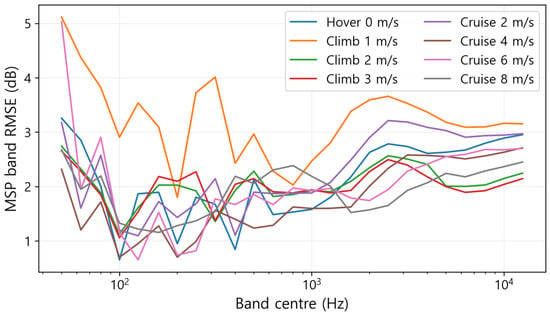
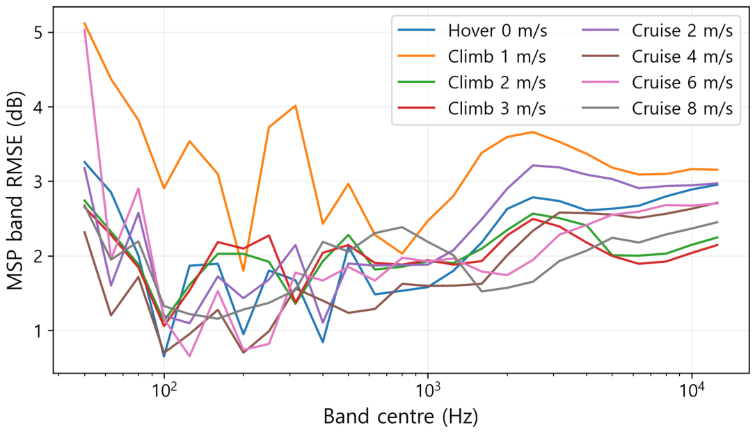
Errors at band level exceed those at the overall level, and vary more widely between conditions. Across conditions, pooled band MAE spans 1.1 to 1.9 dB, whereas the 95th-percentile absolute error extends from 4.2 to 7.6 dB. The largest single-band error recorded is 26.8 dB. In seven conditions, these maxima fall inside the weak 50 or 63 Hz bands; for cruise at 4 m/s, the eighth case arises at 10 kHz. Such frequencies do indicate where reconstruction limits arise, yet they do not reveal the physical causes behind them. Because power summation can downweight errors in weak bands, band-level findings appear together with aggregate metrics in Figure 8 and Table A1.
Figure 8.
MSP band RMSE across the 25 supported bands. Weak low-frequency bands and high-frequency tails are retained.
3.3. Additional Interpolation Comparisons and Sensitivity
In Table 6, MSP is set against stronger alternatives. The original three-smoothing RBF gives OASPL MAE of 0.1–0.5 dB, lower than MSP in every state. For RBF-minus-MSP MAE, paired direction-cluster bootstrap intervals all lie below zero (Table A2). At the two-decimal precision used in Table 6, direct dB interpolation has lower OASPL MAE in hover and in all climb states, while MSP has lower OASPL MAE in cruise. These comparisons rest on point estimates. SH performance varies with condition. Such internal angular comparisons lend support to RBF; the default method is assessed separately through external-layout results and operational evidence, as discussed below.
Table 6.
Held-out OASPL MAE (dB), 50 Hz–12.5 kHz. Intervals are 95% direction-cluster bootstrap intervals for the MSP method. SH and RBF use training-only nested selection.
Direct dB interpolation produces a lower pooled band MAE than MSP in all eight states, and RBF lowers it further still. For MSP, restricting integration to 100 Hz–12.5 kHz keeps the rounded overall MAE range at 0.3–0.8 dB. The largest individual-band error falls from 26.8 to 23.9 dB, but remains sizeable. Figure 8 shows the MSP band RMSE; pronounced error tails continue above 100 Hz.
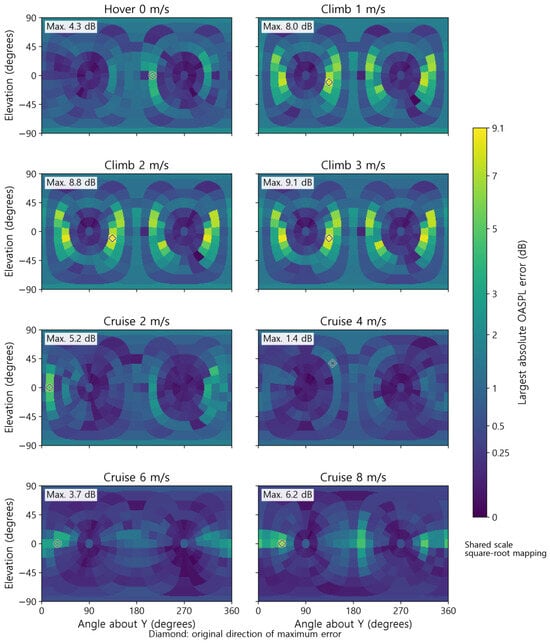
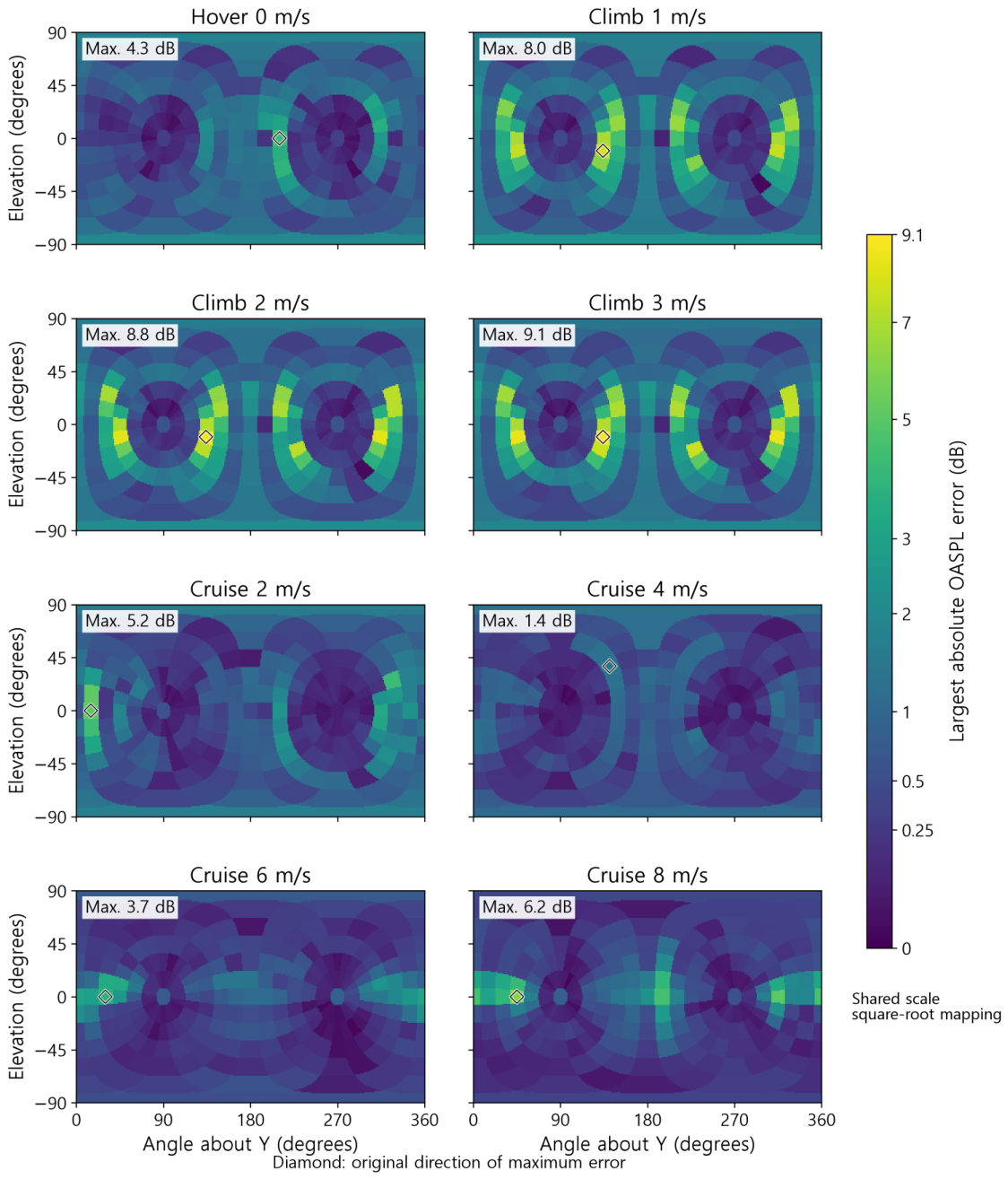
During climb at 3 m/s, the global maximum was recorded: a positive error of 9.1 dB. In each of the three climb fields, the worst-case error aligned with the direction of the same original signed tuple. This position lies outside the rotor plane, and the plotted elevation follows the corrected Y-vertical definition. Rather than indicating uniform reconstruction quality, Figure 9 draws attention to localised concentrations of error. When partitions are identical, endpoint sign retention under holdout predictions is given as 97.6% for cruise changes of no less than 1 dB and as 98.4% for climb changes of no less than 1 dB. These descriptive changes are interpreted within the reconstruction limits.
Figure 9.
Largest absolute MSP OASPL reconstruction error at each original held-out direction across five repetitions. Coordinates retain signed reference axes; these are reduced-density errors relative to computed source spectra. Piecewise-constant spatial heatmaps assign each display cell the value at the nearest original direction on the sphere. All panels share the same colour scale with square-root mapping; diamonds mark the original maximum-error directions. Display sampling does not add acoustic resolution.
3.4. Directional Representation Loss
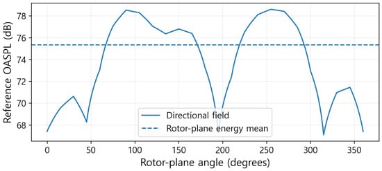
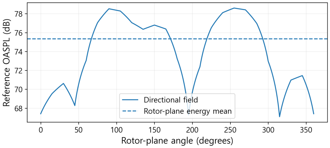
Scalar MAE values of 1.6–2.7 dB and nearest-direction MAE values of 0.6–1.1 dB appear in Table 5, with MSP MAE of 0.3–0.8 dB serving as the benchmark. The scalar energy mean displays no directional dependence, yet the nearest lookup method, although it preserves the sampled spectra, is discontinuous between them. The fact that these two computed-field baselines yield larger errors underscores the advantages of reconstructing directivity. Even so, no conclusion regarding the physical accuracy of the underlying source can be drawn from these results. The directional information that a scalar source representation discards is shown in Figure 10.
Figure 10.
Cruise-8 rotor-plane OASPL and its energy-mean scalar representation. This is information loss within the computed field, not an error against an experiment.
3.5. Ground-Directed Transfer at Full Source Density
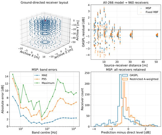
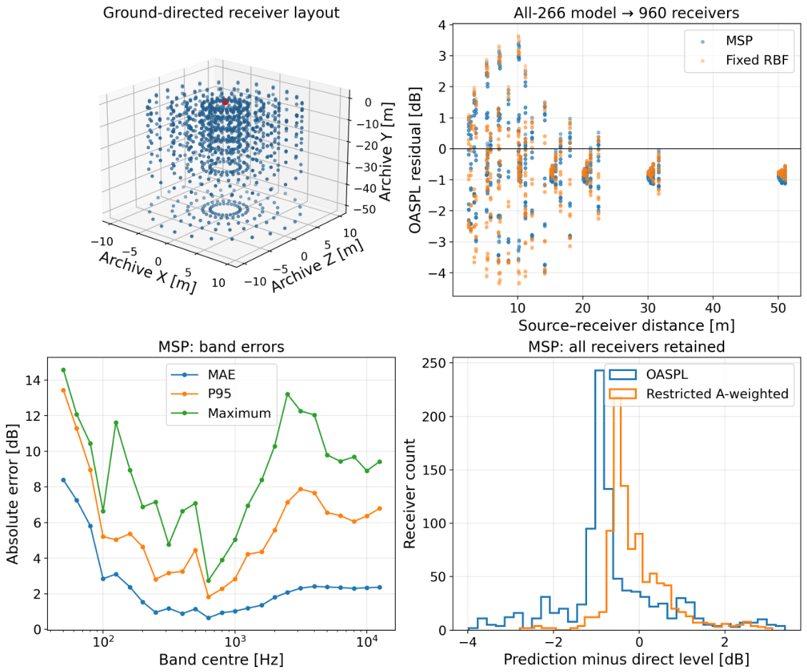
For the full-density database, Table 7 sets out the layout-transfer evaluation, which is reported separately from grouped holdout results obtained by training with roughly 80%. In the case of MSP, the OASPL MAE attained 1.11 dB; the absolute error at the 95th percentile stood at 2.91 dB and the maximum absolute error was 3.98 dB. Inside the restricted band, the A-weighted level MAE was 0.57 dB. Because the largest absolute error within any single band came to 14.58 dB, these averaged quantities ought not to be read as evidence of accuracy in every band. When frequencies below 100 Hz were excluded, the pooled band MAE fell from 2.44 to 1.80 dB, and yet a single-band maximum of 13.21 dB remained. Consequently, both low- and higher-frequency tails must be reported explicitly.
Table 7.
External-layout errors at all 960 receivers. A-weighted levels are restricted to 50–12,500 Hz. P95 and maximum denote absolute errors. The fixed and training-selected RBF comparisons were not tuned on these receivers.
When the input is restricted to complete source data, the chosen cubic RBF returns OASPL MAE equal to 1.20 dB, alongside P95 equal to 3.57 dB; its restricted A-weighted MAE is 0.55 dB. Hence, the mixed ranking of MSP and RBF remains unchanged if RBF selection is carried out through a broader search confined to source data, instead of depending only on the initial fixed configuration.
Within the set of 960 receivers, 948 lay at directions whose separation from the nearest database direction exceeded . This tolerance served to identify angular coincidence arising from rounding of coordinate output and was not intended as a threshold for accepting errors. For that subset, comprising 948 receivers, the MSP OASPL MAE was 1.10, the P95 was 2.87, and the maximum was 3.76 dB. By contrast, the other 12 receivers that displayed angular coincidence gave an OASPL MAE of 2.25 dB, with a maximum error of 3.98 dB. Discrepancies at coincident directions cannot be explained by angular interpolation on its own. Possible sources include near-field effects, finite recording support, and the treatment of retarded time, yet no single cause has been shown to dominate. In addition, these queries are not 948 independent source realisations, and they are not necessarily 948 mutually distinct directions. The receiver layout, together with transfer residuals, appears in Figure 11.
Figure 11.
Transfer from the complete 266-direction climb-2 database to 960 direct receiver spectra: receiver geometry, OASPL residuals versus distance, per-band absolute errors and MSP residual distributions. The negative-Y layout was designed for ground-directed downward propagation and is non-spherical and non-uniform. The red marker denotes the source reference point at the archive origin. All receivers are retained in the primary summaries.
3.6. Expanded RBF, Triangle Quality and Field Integrals
Once the declared numerical guards were in place, searching over 36 candidates gave RBF OASPL MAE of 0.09–0.44 dB. Some local zero-smoothing fits that ran without such guards produced nonphysical magnitudes; omitting these is required in practice, and it does not provide evidence that RBF is generally superior. Table 8 retains the error tails. Enlarging the tested set cannot establish that any kernel or parameter setting is globally optimal.
Table 8.
Expanded training-selected RBF errors (dB), using identical repeated angular partitions. The individual-band maximum is reported separately from OASPL.
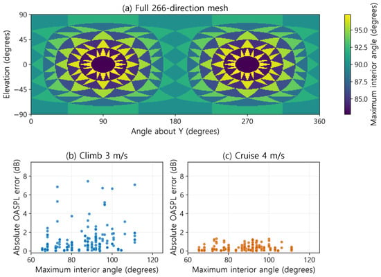
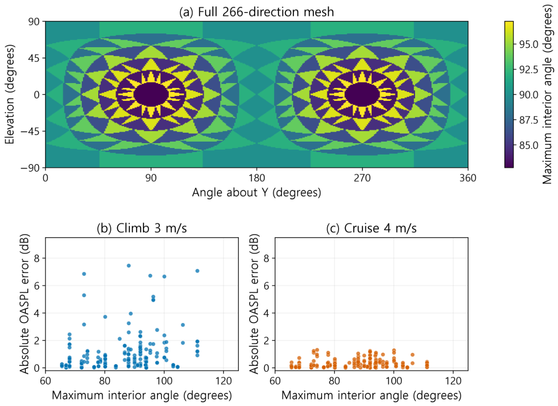
Held-out maximum interior angles ranged from 65.5 to 118.9 degrees. Their Spearman correlation with absolute MSP OASPL error was 0.17–0.39 across states. These correlations link geometry to error risk but do not identify triangle shape as the sole cause. Climb fields share local minima along weak directions. Convex MSP mixtures fill these minima with larger neighbouring powers, yielding positive errors at the common worst direction. Angular sampling is identical across regimes, but source-field contrast differs. At the worst climb-3 direction, reference OASPL was 62.90 dB; triangle vertex levels were 72.06, 63.88 and 71.98 dB. This contrast supports an interpolation mechanism for concentrated climb errors, without isolating an aerodynamic cause. The shortest climb-1 record raises temporal concerns, but its duration is not shown to cause all climb errors. Figure 12 shows full-density triangle quality and angle–error associations for the two illustrated states.
Figure 12.
(a) Spatial heatmap of maximum great-circle interior angle, with a constant value within each full-density spherical triangle. (b,c) Angle versus held-out MSP OASPL error for climb 3 m/s and cruise 4 m/s, shown separately for the first repeated partition. Other repetitions enter the reported correlations.
In the total-energy surrogate, MSP levels integrated from source-Voronoi and dense-sphere treatments differed by to 0.009 dB, the greatest band change being 0.121 dB. For the chosen RBF, total changes lay between and 0.021 dB, and the greatest band change came to 0.087 dB. Differences in quadrature consistency this small neither prove exact conservation nor establish that squared near-field pressure is equivalent to acoustic sound power. Conversion to sound power or NPD calls for a validated convention covering propagation and reference. Setup, batch and single-query costs, as well as array storage, are given in Table 9.
Table 9.
Full-density query costs on the test workstation. Setup is reported separately. Batch times are medians of five warm 1000-query evaluations; single-query times are medians of 50 calls. Each selected RBF uses a cubic kernel and zero smoothing; n is its neighbour count. Array storage excludes library structures and process peak memory.
For hover and cruise at 4 and 8 m/s, slower RBF batches relied on 64 neighbours, whereas 32 neighbours were used in the remaining states; every case applied the same cubic kernel with zero smoothing. Higher query cost accompanies larger local fits, but this benchmark cannot disentangle neighbourhood size from query geometry and solver overhead.
Within this implementation, MSP delivers a measured advantage for warm batches, circumvents kernel selection, and preserves convex, non-negative band-energy mixtures. By contrast, RBF achieves better internal angular accuracy, yet it demands local polynomial conditioning and selection. For the present archive and ground-directed use, MSP remains the default: the 960-point assessment yielded lower OASPL and P95 errors than either fixed or full-training-selected RBF, even though both RBF options slightly lowered the mean restricted A-weighted error. This decision rests on mixed evidence; it does not claim sound-power conservation or uniformly superior MSP accuracy. In addition, the benchmark evaluates neither CFD-generation cost nor real-time performance for complete UAM applications.
3.7. Withheld Interior Operating States
The complete state holdout results appear in Table 10.
Table 10.
Complete-state holdouts by equal energy interpolation between bracketing same-mode states, evaluated at 266 directions. All errors are in dB.
The interior-state test yielded OASPL MAE 0.42–1.18 dB, substantially exceeding some errors that stem only from angle. Individual-band maxima attained 43.90 dB, which shows that helpful overall-level interpolation can mask a weak band’s failure. These computations use withheld states, but they lie within speed ranges already covered; validation extends to no further CFD state, RPM, attitude, or other platform. The speed-based energy mixture does not reproduce each rotor’s control schedule: for example, the second listed rotor (zone 16) fell from 6881 RPM at cruise 4 m/s to 6776 RPM at 6 m/s. Hence, the interpolation does not establish an independently validated RPM-dependent response.
3.8. Outdoor Altitude Comparison
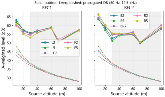
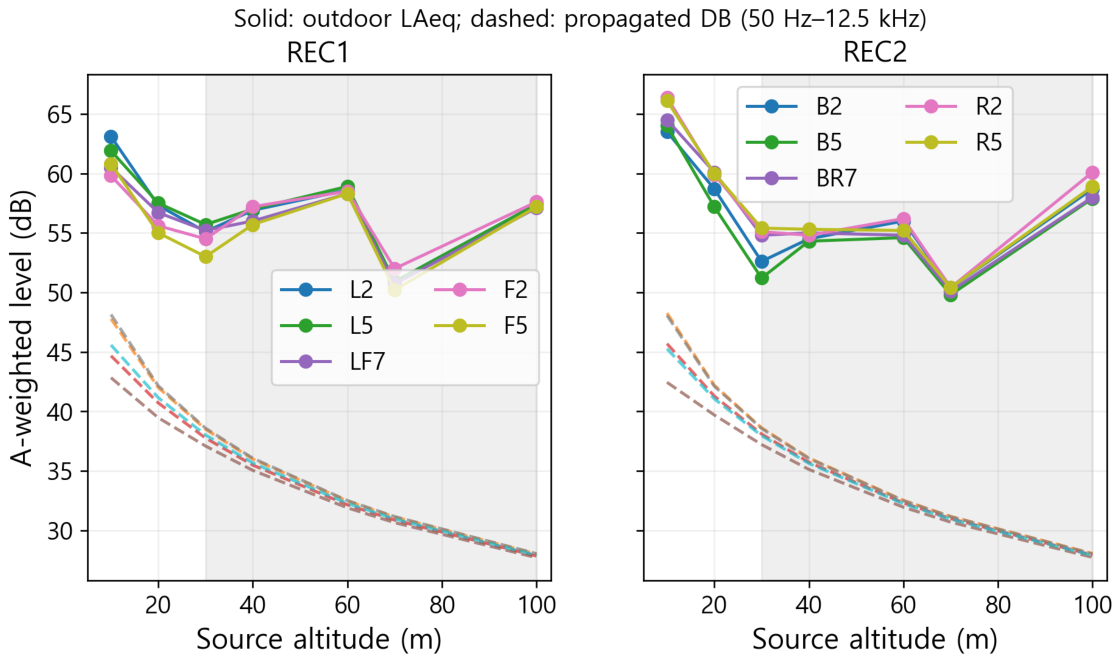
Outdoor hover measurements are set against database values that have been propagated to the matching nominal microphone positions in Figure 13; no source-level offsets are fitted. For source altitudes of 10 and 20 m, the mean measured-minus-predicted difference across each recorder sequence is 15.3–19.0 dB (Table 11). This discrepancy argues against assertions that a low angular MAE is sufficient to establish absolute accuracy outdoors. Because the difference also incorporates changes in operating conditions, spectral bandwidth, background and propagation, it cannot be ascribed exclusively to CFD amplitude error.
Figure 13.
Outdoor equivalent A-weighted levels and propagated hover database levels at seven source altitudes. Dashed predictions use the common 50 Hz–12.5 kHz band set. Grey shading marks the altitude range reported as background limited. REC1 and REC2 are separate recorder sequences, not independent replications of identical acoustic conditions.
Table 11.
Outdoor minus propagated restricted-band A-weighted level at 10 and 20 m (dB). Each entry uses five microphone sites; the reference geometry uses 1.5 m microphone height and the signed ground-axis alignment.
If the sampled heading sensitivities are considered alongside those for height at 1.2–1.5 m, then the smallest measured-minus-predicted discrepancy recorded at 10–20 m is 11.54 dB. At the sites assessed, changes in the stated atmospheric sensitivity alter the upper predicted level by at most 0.45 dB, so the mismatch remains unresolved. Rather than being derived from meteorological data gathered during the campaign, these sensitivity parameters are assumed. In view of the nonmonotonic behaviour seen in high-altitude observations and the documented background constraints, their residuals cannot be taken as evidence of aircraft-source error alone.
4. Discussion
4.1. Evidence for Database Use
Results from angular holdouts show that directional spectra retain information that scalar representations discard. Enlarging the RBF search lowers internal angular errors, yet downstream method selection is also constrained by tail errors, conditioning, integration consistency, and query cost. Full-density evidence at new locations comes from the comparison using the 960 receivers, which share the same CFD source; this bounds the combined directional/radial transfer, but it does not provide an independent check on source aerodynamics. Complete-state holdouts do support interpolation within the sampled speed ranges, although substantial band tails mean that unqualified spectral prediction should be treated with caution.
The outdoor comparison evaluates the physical chain from source through propagation on its own terms. Rather than removing the considerable positive measured-minus-predicted discrepancy through calibration, that discrepancy is kept. An outcome of this kind is compatible with a low reconstruction MAE because reconstruction compares different representations of one and the same computed field. Among the possible causes are source operating mismatch, high-frequency broadband noise not present in the CFD source, ground interaction, measurement and background effects, and limited prediction bandwidth; which of these predominates has not been determined. Even where the documented nominal geometry is specified, supplementary receiver-level spectra preserve broadband and amplitude differences; they offer no validation under matched operating conditions.
4.2. Community Exposure and Transferability
The database provides directional band inputs for the route calculation that follows. Time-dependent source range, direction, and operation are required by events and SEL, while and also call for annual scheduling and night/evening treatment [2,10,12]. For emerging aircraft, guidance ties noise management to stakeholder engagement and governance [15]. Hence, route setbacks, restrictions on operating times, and monitoring depend on validated receiver predictions and the applicable local procedures, not on a source OASPL threshold. Frequency-dependent weighting and absorption are enabled by a band database, although narrowband recordings are still required for tonality and temporal psychoacoustic metrics [11]. Neither social acceptance nor legal compliance follows from the present data.
A framework for source-to-event-to-exposure calculations is provided by SAE AIR1845A, together with the AEDT workflow, though this does not establish that every airplane approximation holds for small drones. The usual source-spectrum range of AEDT covers 50 Hz–10 kHz, in contrast to the 50 Hz–12.5 kHz range commonly used here [12]. Spectral assessment for this platform is supported by the additional 12.5 kHz band, whereas unsupported 16/20 kHz inventory values are left out. To convert to a given NPD implementation, weighting, frequency limits, operation/power indexing, directivity and reference propagation must all be reconciled.
Scaling laws for passenger eVTOL aircraft, ducted fans, tilt-rotors or six-/eight-rotor vehicles are not established by the rotor speeds and dimensions of the four-rotor X500 configuration. Fresh source fields must be generated for each case because blade count, tip Mach number, rotor interactions, installation, and control state may all vary. The schema and reconstruction procedure are reusable across platforms; absolute levels and directivity, however, cannot be transferred unless validation is performed separately [6,7,8].
4.3. Limits of the Present Assessment
Across all bands, far-field applicability of the approximately 1 m acquisition sphere has not been established; both source-size/aperture and reactive-term criteria apply. Computed downward-transfer evidence exists only for the specific radii and sectors sampled. This investigation evaluates the representation and reconstruction of directional source spectra that already exist. It incorporates neither a coupled urban propagation model accounting for ground impedance, buildings, or meteorological refraction, nor a new study on CFD source convergence. The description of atmospheric sensitivity pertains to a single downstream interface and does not confirm residential accuracy or compliance.
The contiguous record blocks measure sensitivity to the retained histories of 0.06–0.11 s, rather than reflecting independent temporal statistics. Their short duration limits their usefulness for interpreting low frequencies. Operating inputs used in the assessment are specified by Table 2 and the common solver description. Angular MAE characterises the error in reduced-density computed-field reconstruction, whereas the 960-location test describes the error in full-density layout-transfer. Neither metric represents an independent result for CFD convergence.
The derived data and code used here (source spectra, fold assignments, external transfer arrays, outdoor comparison tables, calculation kernels and plotting code) allow the database analyses to be re-evaluated; they were made available to the reviewers during peer review but are not publicly released. Public access to the raw experimental recordings and the underlying CFD files is also restricted by project ownership and governing agreements. Consequently, the representation and reconstruction analyses can be reproduced only with access to these materials, and no claim is made that the flow solution can be independently regenerated. For legacy outdoor comparisons, observation-specific background and operating records are irrecoverable; measured discrepancies therefore serve only as observational checks, and not as calibrated demonstrations of accuracy.
5. Conclusions
Angular holdouts, previously withheld interior states, newly introduced receiver locations, and outdoor hover observations are used to assess an eight-state, directional spectral database for X500 that spans a common range from 50 Hz to 12.5 kHz. By comparing scalar MAE (1.6–2.7 dB) with nearest-direction MAE (0.6–1.1 dB), directivity contributions within these computed fields are quantified; both values exceed the reduced-density angular MAE of MSP (0.3–0.8 dB). The angular MAE is furthermore reduced to 0.09–0.44 dB when expanded, guarded RBF is applied with explicit parameter selection and stability checks.
Tail behaviour is poorly captured by mean errors: there, MSP angular P95 attains 3.3 dB, the maximum OASPL error is 9.1 dB, and the largest band error reaches 26.8 dB. When all 266 source directions are transferred to the 960 ground-directed receivers, the resulting OASPL MAE/P95/maximum values are 1.11/2.91/3.98 dB, together with a restricted A-weighted MAE of 0.57 dB. In view of this mixed external evidence, measured warm-query costs and an untuned convex energy representation, MSP remains the default choice for ground-directed applications; exact conservation of sound power is not asserted, however.
Complete-state holdouts produce OASPL MAE of 0.42–1.18 dB across the established speed intervals, even though maxima for individual bands attain 43.90 dB. Such results therefore lend support to bounded state interpolation; they do not, however, demonstrate any capacity for extrapolation to fresh RPMs, attitudes, or aircraft types. When the verified Y-vertical convention is adopted, physical-plane descriptions and plots are altered, while the registered reconstruction calculations remain unaffected.
Physical outdoor comparisons at 10 and 20 m reveal mean discrepancies of 15.3–19.0 dB. The validation outcome is thus unfavourable, since accurate, absolute prediction of community noise has not been shown. Neither residential compliance nor absolute source accuracy is confirmed by this test; for those purposes, a separately validated chain covering both source and propagation is required. This database could nonetheless act as a source-data component in later NPD and exposure calculations, provided that any conversion conforms to conventional source ranges (50 Hz–10 kHz), the 12.5 kHz extension that the dataset supports, weighting schemes, operating-state indexing, and event geometry.
Author Contributions
Conceptualisation, S.R.; methodology, S.R. and D.C.; formal analysis, S.R.; validation and experimental methodology, J.K.; software and interpolation, H.K.; data curation, S.R.; writing—original draft preparation, S.R.; writing—review and editing, all authors; visualisation, S.R.; supervision, S.K.; project administration, S.K.; funding acquisition, S.K. All authors have read and agreed to the published version of the manuscript.
Funding
This research was supported by the Korean Urban Air Mobility (K-UAM) Safety Operation System Core Technology Development Project through the Ministry of Land, Infrastructure and Transport (MOLIT) and the Korea Agency for Infrastructure Technology Advancement (KAIA) (RS-2024-00405707), and by the Basic Science Research Program through the National Research Foundation of Korea (NRF), funded by the Ministry of Education (RS-2020-NR049595).
Institutional Review Board Statement
Not applicable; this study uses computational and acoustic data and does not involve human or animal subjects.
Informed Consent Statement
Not applicable.
Data Availability Statement
Raw experimental recordings and the underlying CFD files cannot be shared publicly because of project ownership and agreements. The derived data and code used for the database construction, reconstruction and receiver-comparison analyses, comprising calculation and plotting code, prediction arrays, evaluation assignments and derived spectra, are likewise not publicly released; they were made available to the reviewers during peer review. These materials do not permit independent regeneration of the CFD solution.
Conflicts of Interest
The authors declare no conflicts of interest.
Abbreviations
The following abbreviations are used in this manuscript:
| UAM | Urban air mobility |
| CFD | Computational fluid dynamics |
| FW–H | Ffowcs Williams–Hawkings |
| SPL | Sound pressure level |
| OASPL | Overall sound pressure level |
| MRF | Multiple reference frame |
| RPM | Revolutions per minute |
| ARD | Acoustic receiver data (pressure-history file) |
| ROC1 | Climb-at-1-m/s archive group |
| NPD | Noise–power–distance |
| AEDT | Aviation Environmental Design Tool |
| MAE | Mean absolute error |
| RMSE | Root mean square error |
| P95 | 95th percentile of absolute error |
| SH | Spherical harmonics |
| RBF | Radial-basis function |
| HRTF | Head-related transfer function |
| MSP | Mean-square-pressure interpolation |
| SEL | Sound exposure level |
| JSON | JavaScript Object Notation |
Appendix A. Supplementary Reconstruction and Spectral Evidence
Appendix A.1. Band-Level Reconstruction Errors
Table A1.
Pooled band-level reconstruction errors in dB over 25 complete bands and five grouped cross-validation repetitions. Each state has 33,250 band comparisons from 266 original directions. P95 and maximum refer to absolute errors.
Table A2.
Paired direction-cluster bootstrap differences in OASPL MAE for the original training-selected, three-smoothing RBF minus MSP (dB), using the same 25-band angular evaluation. Intervals are conditional 95% intervals from 2000 direction-cluster resamples; negative values favour RBF.
Appendix A.2. Pressure-History Temporal Support
The audit includes all 266 receiver histories in each state. Across individual records, the largest relative deviation of reported sample intervals stays under 0.00036. Record durations and nominal FFT spacings, obtained from mean intervals, appear in Table 3. A statistically converged band level is not verified by either an available FFT bin or a finite band entry. Interpretation at low frequencies is limited by short record lengths, and by the presence of merely one or two bins inside the 50 Hz band.
Appendix A.3. Supplementary Measured and Calculated Spectra
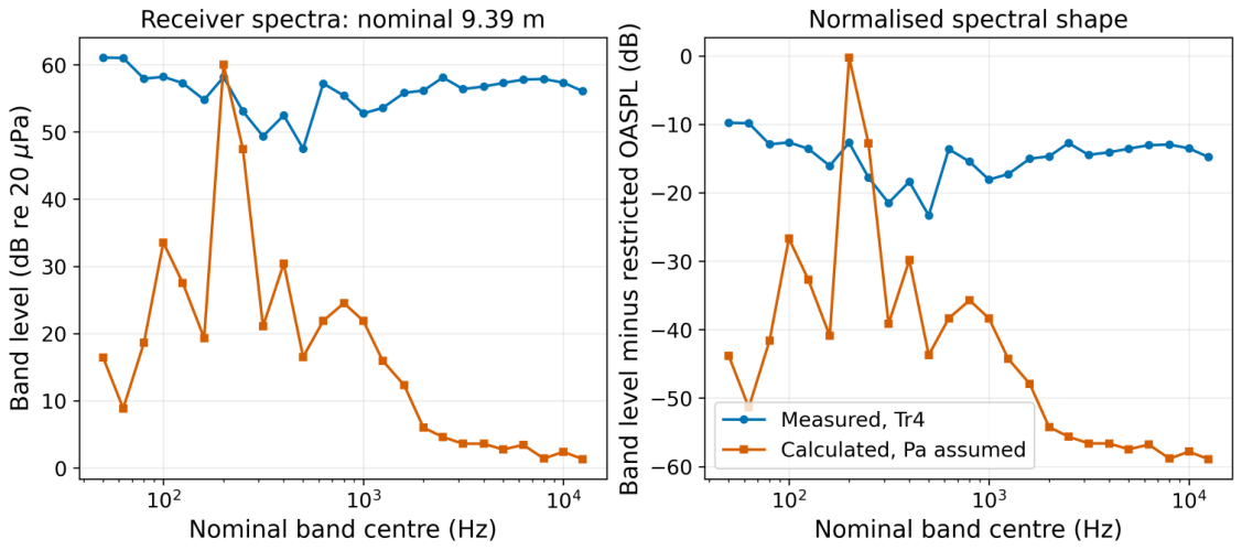
A supplementary comparison at receiver level makes use of a legacy hover setup, with a source height of 10 m, a horizontal receiver offset of 4 m, and a microphone height of 1.5 m; the resulting nominal source–receiver range is m. The measured signal is that of the distance-labelled fourth recorder track, whereas the calculated export pertains to the documented receiver setup. Neither signal is the same as the 1 m database spectra, nor do they form the altitude-transfer residuals presented in Table 11. Mean-removed Hann–Welch spectra are computed with 16,384-sample windows, a 65,536-point FFT, and 50% overlap. In the case of the measured five-second signal, retained 94 dB calibrator scaling is applied, although its channel-specific transfer has not been established independently; by contrast, the calculated float-pressure signal is interpreted in Pa. Restricted Z/A totals are 70.84/68.11 dB for the measured track and 60.24/49.57 dB for the calculated export. Synchronised operating conditions and matched calibration cannot be established from the nominal receiver geometry. Consequently, broadband and amplitude differences are kept as a supplementary diagnostic and are not treated as independent verification of accuracy. Absolute and normalised receiver spectra are compared in Figure A1.
Figure A1.
Supplementary measured and calculated one-third-octave receiver spectra for the stated nominal 9.39 m hover geometry and processing assumptions. The absolute and normalised views retain spectral-shape differences; nominal geometry does not establish matched operating conditions.
References
- SAE International. AIR1845A: Procedure for the Calculation of Airplane Noise in the Vicinity of Airports; SAE: Warrendale, PA, USA, 2012. [Google Scholar] [CrossRef] [Scilit]
- Rizzi, S.A.; Letica, S.J.; Boyd, D.D.; Lopes, L.V. Prediction of noise-power-distance data for urban air mobility vehicles. J. Aircr. 2024, 61, 166–182. [Google Scholar] [CrossRef] [Scilit]
- Rizzi, S.A.; Rafaelof, M. On the modeling of UAM aircraft community noise in AEDT helicopter mode. In Proceedings of the AIAA AVIATION Forum, San Diego, CA, USA, 12–16 June 2023. [Google Scholar] [CrossRef] [Scilit]
- Jo, Y.; Cho, H.I.; Jeon, W. Development of a community noise assessment code for rotorcraft using a noise hemisphere. In Proceedings of the KSAS Spring Conference, Goseong, Republic of Korea, 20–22 April 2022; pp. 192–194. [Google Scholar]
- Pascioni, K.A.; Page, J.A.; Boyle, D.K. UAM Source Noise Hemisphere Flight Test Measurement Protocol; NASA/TM-20240011587; NASA Langley Research Center: Hampton, VA, USA, 2024. Available online: https://ntrs.nasa.gov/citations/20240011587 (accessed on 12 November 2026).
- Zawodny, N.S.; Boyd, D.D., Jr.; Burley, C.L. Acoustic characterization and prediction of representative, small-scale rotary-wing unmanned aircraft system components. In Proceedings of the AHS International 72nd Annual Forum, West Palm Beach, FL, USA, 17–19 May 2016. [Google Scholar]
- Intaratep, N.; Alexander, W.N.; Devenport, W.J.; Grace, S.M.; Dropkin, A. Experimental study of quadcopter acoustics and performance at static thrust conditions. In Proceedings of the 22nd AIAA/CEAS Aeroacoustics Conference, Lyon, France, 30 May–1 June 2016. [Google Scholar] [CrossRef] [Scilit]
- Schäffer, B.; Pieren, R.; Heutschi, K.; Wunderli, J.M.; Becker, S. Drone noise emission characteristics and noise effects on humans—A systematic review. Int. J. Environ. Res. Public Health 2021, 18, 5940. [Google Scholar] [CrossRef] [Scilit] [PubMed]
- Heutschi, K.; Ott, B.; Nussbaumer, T.; Wellig, P. Synthesis of real world drone signals based on lab recordings. Acta Acust. 2020, 4, 24. [Google Scholar] [CrossRef] [Scilit]
- World Health Organization Regional Office for Europe. Environmental Noise Guidelines for the European Region; WHO: Copenhagen, Denmark, 2018; ISBN 978-92-890-5356-3; Available online: https://www.who.int/europe/publications/i/item/9789289053563 (accessed on 12 November 2026)ISBN 978-92-890-5356-3.
- Boucher, M.A.; Christian, A.W.; Krishnamurthy, S.; Tracy, T.; Begault, D.R.; Shepherd, K.; Rizzi, S.A. Toward a Psychoacoustic Annoyance Model for Urban Air Mobility Vehicle Noise; NASA/TM-20240003202; NASA: Hampton, VA, USA, 2024. Available online: https://ntrs.nasa.gov/citations/20240003202 (accessed on 12 November 2026).
- Federal Aviation Administration. Aviation Environmental Design Tool (AEDT), Version 4b; Technical Manual. FAA: Washington, DC, USA, 2026. Available online: https://aedt.faa.gov/Documents/AEDT4b_TechManual.pdf (accessed on 12 November 2026).
- Broatch, A.; Navarro, R.; García-Tíscar, J.; Ramírez, F.N. Evaluation of different FW-H surfaces and modal decomposition techniques for the acoustic analysis of UAV propellers through detached eddy simulations. Aerosp. Sci. Technol. 2024, 146, 108956. [Google Scholar] [CrossRef] [Scilit]
- Fasulo, G.; Longobardo, G.; De Gregorio, F.; Barbarino, M. Experimental acoustic investigation of rotor noise directivity and decay in multiple configurations. Aerospace 2025, 12, 647. [Google Scholar] [CrossRef] [Scilit]
- UK Civil Aviation Authority. Managing Noise from Emerging Aviation Technology; CAP3304, Version 1; CAA: Crawley, UK, 2026; Available online: https://www.caa.co.uk/data-and-publications/publications/documents/content/cap3304/ (accessed on 12 November 2026).
- Bau, D.; Arend, J.M.; Pörschmann, C. Estimation of the optimal spherical harmonics order for the interpolation of head-related transfer functions sampled on sparse irregular grids. Front. Signal Process. 2022, 2, 884541. [Google Scholar] [CrossRef] [Scilit]
- Ryu, S.; Choi, D.; Kwon, J.; Kim, S. Computational analysis-based noise model for urban air mobility considering social acceptance. In Proceedings of the 2025 Asia-Pacific International Symposium on Aerospace Technology, Seoul, Republic of Korea, 27–29 October 2025. [Google Scholar]
- Ryu, S.; Choi, D.; Kwon, J.; Lee, S.; Kim, S.; Tark, H.; Kim, S. Overview of noise prediction model framework based on standards and regulations for UAM corridor evaluation. In Proceedings of the 2025 KSAS Fall Conference, Goseong, Republic of Korea, 11–14 November 2025; pp. 1060–1061. [Google Scholar]
- Ffowcs Williams, J.E.; Hawkings, D.L. Sound generation by turbulence and surfaces in arbitrary motion. Philos. Trans. R. Soc. A 1969, 264, 321–342. [Google Scholar] [CrossRef] [Scilit]
- Farassat, F. Derivation of Formulations 1 and 1A of Farassat; NASA/TM-2007-214853; NASA Langley Research Center: Hampton, VA, USA, 2007.
- ISO 266:1997; Acoustics—Preferred Frequencies. ISO: Geneva, Switzerland, 1997.
- ISO 9613-1:1993; Acoustics—Attenuation of Sound During Propagation Outdoors—Part 1: Calculation of the Absorption of Sound by the Atmosphere. ISO: Geneva, Switzerland, 1993.
- SciPy Developers. SciPy 1.13.1 Reference Guide: RBFInterpolator. 2024. Available online: https://docs.scipy.org/doc/scipy-1.13.1/reference/generated/scipy.interpolate.RBFInterpolator.html (accessed on 12 November 2026).
- ISO 1996-1:2016; Acoustics—Description, Measurement and Assessment of Environmental Noise—Part 1: Basic Quantities and Assessment Procedures. ISO: Geneva, Switzerland, 2016.
- ISO 1996-2:2017; Acoustics—Description, Measurement and Assessment of Environmental Noise—Part 2: Determination of Sound Pressure Levels. ISO: Geneva, Switzerland, 2017.

Disclaimer/Publisher’s Note: The statements, opinions and data contained in all publications are solely those of the individual author(s) and contributor(s) and not of MDPI and/or the editor(s). MDPI and/or the editor(s) disclaim responsibility for any injury to people or property resulting from any ideas, methods, instructions or products referred to in the content. |
© 2026 by the authors. Licensee MDPI, Basel, Switzerland. This article is an open access article distributed under the terms and conditions of the Creative Commons Attribution (CC BY) license.