Hierarchical Quadruped Navigation with Risk and Cost Evaluation: Simulation Validation on Unstructured Terrain for Lunar Missions

Abstract

Quadruped navigation for future lunar missions requires route selection over unstructured terrain that accounts for terrain characteristics and controller execution capabilities. Fixed geometric rules cannot fully capture controller-specific execution risks and time costs. We propose hierarchical navigation based on risk and execution cost evaluation, using regional elevation maps and controller closed-loop data to build local execution and subsequent route-time models. These predict the execution risk and execution time of reaching candidate local goals and the subsequent route time to the task goal, respectively. A deterministic selector combines both stages’ time costs under tiered risk constraints to select each local goal, and a residual local planner tracks the selected goal in closed loop. Upon local-goal arrival, selection repeats until the task goal is reached. Simulations under terrestrial gravity and rigid contact use two low-level controllers to evaluate navigation performance and adaptability to controller changes. The configuration using the first controller achieves 100% success across 108 episodes comprising 36 unstructured-terrain tasks and three evaluation seeds. Ablations show that local execution-risk prediction, subsequent route evaluation, and tiered risk-constrained selection contribute to task completion. With the navigation architecture and hyperparameters fixed, the system adapts to another controller by collecting new closed-loop data and constructing controller-specific models, achieving 93.52% success and producing different detour and obstacle-crossing routes on the same terrain. The results show that the proposed method enables global route selection to adapt to controller-specific execution capabilities, providing a basis for adaptation to lunar locomotion controllers and navigation validation under lunar conditions.

1. Introduction

As lunar exploration expands toward south-polar resource prospecting, exploration of multiple sites, and long-term operations, mobile robots must enter complex regions with dense craters and substantial terrain relief. Having completed its orbiting, landing, and sample-return objectives [1,2], China’s lunar exploration program is advancing toward a new phase centered on Chang’e-7’s comprehensive south-polar investigations and the International Lunar Research Station [3,4]. Evidence of polar water ice further increases the scientific and engineering importance of this region [5]. Mobility over complex terrain and autonomous navigation are therefore essential to extending lunar exploration coverage and improving operational efficiency [6].

Existing lunar surface missions mainly use wheeled platforms, which are prone to slip and sinkage on steep slopes, crater rims, and dense rubble [7,8]. Quadrupeds actively select support positions through discrete footholds and can adjust body posture to cross local obstacles, offering a new means of accessing complex regions that restrict wheeled platforms [9,10]. However, reduced lunar gravity and loose regolith alter robot–ground contact conditions, affecting terrain traversal capability and actual execution efficiency. Quadruped navigation over complex lunar terrain must therefore consider both map-scale route selection and robot-scale physical execution capability.

Earth–Moon communication delays and link bandwidth limitations require robots to autonomously select routes and adjust their motion once a task goal is specified [11,12]. Orbital remote sensing, lander observations, and prior rover surveys can provide regional digital elevation models, supplying map-scale structural information for global planning [13,14]. However, the finite resolution of prior maps cannot fully resolve terrain variations at the foot-contact scale, and actual contact states and motion responses also depend on the robot state and low-level controller. Autonomous navigation must therefore use limited map information for global route decisions and real-time motion states for local planning adjustments.

Traditional elevation-map navigation methods typically assess traversability using slope, height differences, roughness, clearance, and robot dimensions, then generate routes through graph search or sampling-based planning. These methods effectively handle prominent obstacles and route connectivity [15]. However, uniform geometric rules cannot fully represent controller-specific execution risks and time costs: geometrically admissible regions may still induce non-foot contact, and routes of similar length may have different execution times because of slope direction, turning maneuvers, and motion state. Previous studies show that rover locomotion mechanisms affect terrain evaluation and planned routes [16], and that quadruped motion-control policies also influence traversability assessment and route selection [17,18,19]. Geometric rules and terrain-cost weights implicitly assume controller capabilities; changes in these capabilities may therefore require recalibration of planning parameters [20].

Recent learned traversability estimators, motion-cost predictors, and forward dynamics models use robot experience to estimate execution outcomes, enabling new approaches to controller-specific planning [18,20]. Previous methods also learn short-range motion outcomes to evaluate planning-graph edges or complete paths [17,21]. However, local planning focuses on nearby motion adjustments and outputs continuous actions, whereas global planning compares route directions, execution risks, and expected times at the map scale. The two differ substantially in spatial scale, decision form, and feedback period. End-to-end navigation must jointly optimize dense local motion feedback and delayed task-completion feedback, increasing the difficulty of credit assignment and multi-objective optimization [22]. Previous studies use motion models of different fidelity for different planning horizons to accommodate both local execution prediction and broader route search [23,24]. Hierarchical systems clarify the responsibilities of global route selection and local motion execution, but route evaluation based on geometric distance, constant-speed assumptions, or manually calibrated terrain costs still cannot accurately reflect controller-specific traversal risks and execution times [14,25].

The combination of risk and route efficiency also affects the final decision. Some planners combine terrain risk, route length, execution time, and other metrics into a weighted cost and select the route with the lowest total cost [17,26]. However, quantities with different units and meanings complicate weight calibration, while summarizing stochastic outcomes through expected cost may overlook low-probability, high-consequence events [27]. For missions emphasizing reliability, such as lunar surface exploration, planning must first satisfy execution-safety requirements and then optimize route efficiency. Risk measures and risk-constrained planning provide a basis for this relationship between safety and efficiency [23].

Motivated by lunar missions, this paper proposes hierarchical quadruped navigation based on risk and execution cost evaluation and validates it on unstructured terrain in simulation. Regional elevation maps and controller-specific closed-loop data are used to build local execution and subsequent route-time models, respectively evaluating the execution risk and time of reaching candidate local goals and the subsequent route time from candidate positions to the task goal. A deterministic selector combines execution costs from both stages under tiered risk constraints to select a local goal. A recurrent residual local planning policy combines nearby terrain and real-time motion states for closed-loop tracking. Local-goal arrival triggers the next selection, repeating until the task goal is reached.

The main contributions are as follows:

1.

A controller-specific local-goal evaluation method based on closed-loop execution outcomes is proposed. Using closed-loop execution data containing diverse dynamic entry states, the method jointly predicts arrival failure risk for one local-goal commitment, non-foot contact risk conditional on successful arrival, and successful execution time, thereby evaluating the executability of candidate local goals under that controller. The predicted quantities support risk classification and time comparison for current candidates and provide a controller-specific local execution prior for subsequent route evaluation.

2.

A controller-specific method for evaluating subsequent route risk and time is proposed. Local execution priors are extended to directional states across the map, successful subsequent trajectories supervise movement and turning times, and route-time fields are computed at different risk-admission levels, propagating controller-specific execution time to map-scale route evaluation.

3.

A deterministic local-goal selection method with tiered risk constraints is proposed. Risk information determines candidate eligibility and assigns risk classes to current local goals and risk-admission levels to subsequent routes. Among eligible candidates, the method selects a local goal according to two-stage physical execution time and contact preference, and a strict decrease in remaining route time maintains progress toward the task goal.

This paper evaluates overall performance, the roles of the core modules, transfer to an independent map, and adaptation to different execution capabilities through comparisons with external baselines, module ablations, an independent-map evaluation, a parameter-sensitivity analysis, and comparisons between configurations using two low-level controllers on unstructured-terrain tasks.

The remainder of this paper is organized as follows. Section 2 presents the task definition, system architecture, and component methods. Section 3 describes the experimental setup and evaluation protocol. Section 4 reports overall and independent-map results, external baseline comparisons, module ablations, parameter sensitivity, residual and non-residual configurations, and controller comparisons; it also discusses limitations. Section 5 concludes the paper.

2. Methods

2.1. Task Definition and System Overview

This study considers quadruped goal navigation with a regional elevation map. The task inputs are an elevation map $\mathcal{M}$, robot state $x_t$, and task goal g in world coordinates. The navigation layer outputs body-frame velocity commands $u_t=(v_{x,t},v_{y,t},{\omega }_{z,t})$, which a fixed-parameter low-level controller converts into joint actions. The task succeeds when the robot enters the goal-arrival radius. Physical failure, inability to produce a valid local goal, or expiration of the time limit terminates the episode.

The map, candidates, and route-time computation share an elevation grid $Z\in {\mathbb{R}}^{H\times W}$ with resolution Δ = 0.1 m. After boundary checks, world coordinates are mapped to grid-cell centers, providing a common spatial reference for terrain sampling and route-time queries.

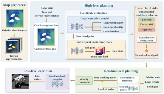
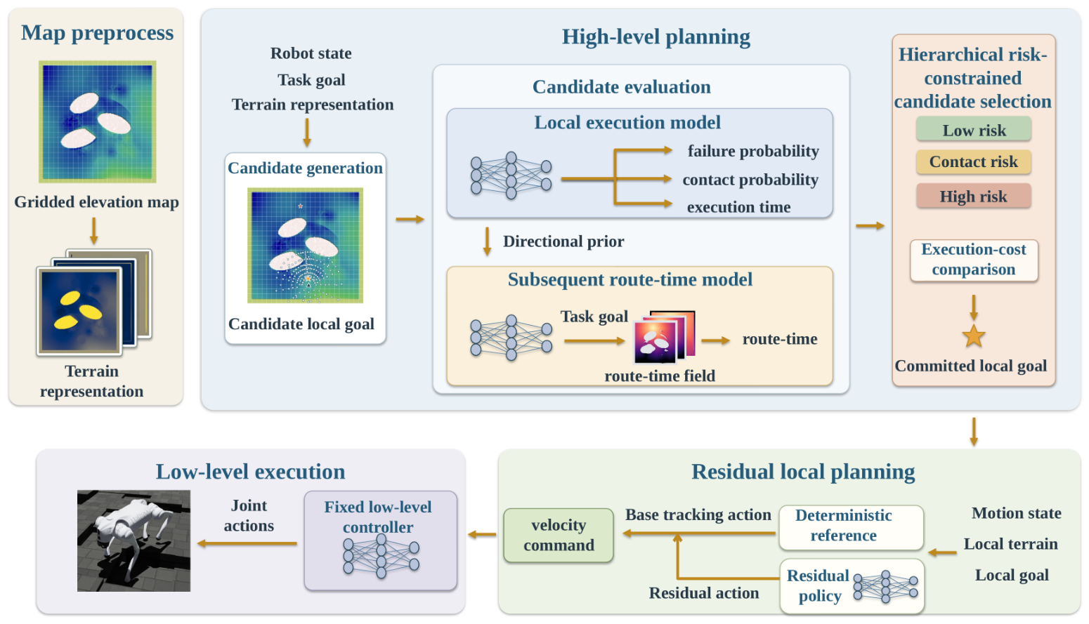
As shown in Figure 1, the system generates directional risk and time priors and computes route-time fields representing the estimated remaining route time to the task goal before task execution. During online decisions, the local execution model predicts the risk and time of reaching each candidate, while subsequent route evaluation estimates the route cost from that candidate to the task goal to assess its global route value. The tiered risk-constrained selector determines a local goal under tiered risk and strict-progress constraints. The residual local planner and low-level controller track this goal in closed loop, and arrival triggers the next decision. Training and precomputation are described in Section 2.6.

Figure 1. Overall system architecture and execution workflow.

2.2. Local-Goal Execution Risk and Time Prediction

The local-goal execution risk and time prediction model predicts arrival probability, non-foot contact probability conditional on successful arrival, and execution time conditional on successful arrival for a single local-goal commitment. Each commitment fixes a local goal, which the residual local planner and low-level controller execute in closed loop until arrival, physical termination, or the prescribed time limit. Hereafter, this model is called the local execution model. The history-encoded form conditions on the current motion state, while the zero-history form represents execution outcomes over the training-state distribution.

At decision step k, given robot state $x_k$, candidate local goal $e_{k,i}$, and elevation map $\mathcal{M}$, the history-encoded model predicts

$$\begin{array}{cc}\hfill P_{A,i}& =P(A_i\mid x_k,e_{k,i},\mathcal{M}),P_{F,i}=1-P_{A,i},\hfill \\ \hfill P_{D,i}& =P(D_i\mid A_i,x_k,e_{k,i},\mathcal{M}),\hfill \\ \hfill {\widehat{t}}_i& =\mathbb{E}[T_i\mid A_i,x_k,e_{k,i},\mathcal{M}].\hfill \end{array}$$

Here, $A_i$ denotes entry into the candidate goal’s handoff radius within the prescribed time limit; $D_i$ denotes a specified non-foot contact involving the body, hip, thigh, or shank during that execution; and $T_i$ is the actual time required to reach the candidate. Thus, $P_F$ is arrival failure probability, $P_D$ is non-foot contact probability conditional on successful arrival, and ${\widehat{t}}_i$ is predicted successful execution time.

The history-encoded model takes motion history, candidate conditions, and three candidate-aligned terrain patches as inputs, as summarized in Table 1. Here, B is the batch size and M is the number of candidates per state.

Table 1. Local execution model inputs.

Input	Shape	Description
Motion history	$[B,10,9]$	10 frames of body linear velocity, angular velocity, and projected gravity
Candidate condition	$[B,M,3]$	Normalized distance and direction cosine and sine
Start terrain patch	$[B,M,6,21,17]$	Nearby terrain involved in turning at the start of execution
Execution terrain band	$[B,M,8,73,17]$	Execution corridor from the current state to the candidate endpoint
Target terrain patch	$[B,M,6,13,17]$	Support conditions and motion space near the candidate endpoint

The three terrain patches cover the initial turning region, the execution corridor to the candidate goal, and the support and motion space after arrival, allowing for terrain conditions to be evaluated at different stages of local execution.

The three patches share five continuous terrain channels and a known-map mask. Relative height uses ground elevation at the robot’s current position as its reference; longitudinal and lateral slopes describe elevation changes along and across the candidate direction; local nonplanarity is computed from elevation residuals after neighborhood plane fitting; and edge strength uses directional second-order elevation differences to extract geometric discontinuities such as crater rims, rock boundaries, and slope breaks. The continuous terrain channels are normalized before model input.

The execution terrain band additionally includes a candidate-length validity mask and normalized longitudinal position, indicating the valid execution region and position along the band. The start terrain patch and target terrain patch therefore each contain six channels, while the execution terrain band contains eight.

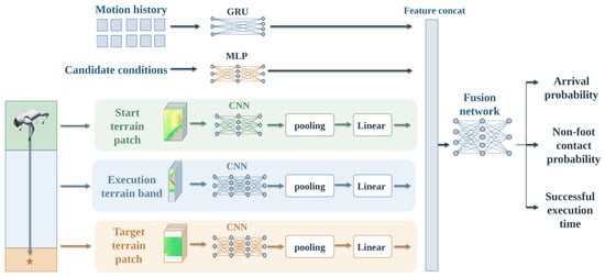
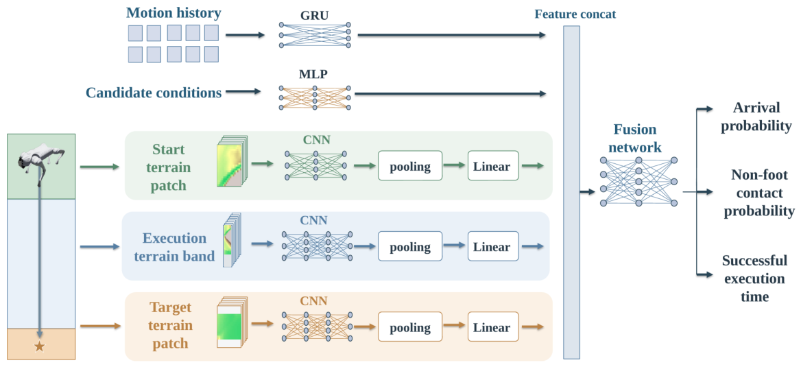
As shown in Figure 2, motion history is encoded by a single-layer GRU with hidden size 64; the zero-history form uses a fixed 64-dimensional zero vector. Candidate conditions pass through a $3\to 32\to 32$ MLP. Independent terrain CNNs use channel widths $(32,64,96)$ for the start patch and $(32,64,96,128)$ for the execution band and target patch, with $3\times 3$ kernels, ELU activations, and downsampling along the longitudinal axis. Structured pooling and linear projection produce respective feature dimensions of 96, 128, and 128.

Figure 2. Network architecture of the local execution model. The history-encoded form is shown.

Within valid sampling regions, structured pooling uses masked means and maxima to extract overall features and strong local responses, longitudinal aggregation and a one-dimensional convolution to encode lateral distributions, and statistics of edge strength on both sides and of the asymmetry between them. The execution terrain band further combines central-region nonplanarity and edge strength to extract responses to short contiguous hazardous segments. These features are fused into terrain vectors.

The motion-state, candidate-condition, and three terrain-branch features are concatenated into a 448-dimensional vector and passed through a $448\to 256\to 128$ fusion network. Three independent heads predict arrival probability, conditional non-foot contact probability, and successful execution time. Probability outputs use sigmoid transformations, and the time output uses a sigmoid transformation multiplied by the execution time limit.

The model is supervised by closed-loop local-goal execution outcomes. Arrival labels cover all samples, while non-foot contact and execution time are supervised only on successful-arrival samples. Let $y_A,y_D,y_T$ denote arrival, non-foot contact, and actual elapsed-time labels, and $z_A,z_D$ the raw outputs of the corresponding probability heads. The per-sample loss is

$${\mathcal{L}}_{\mathrm{ER}}=BCELogit(z_A,y_A)+y_{A}BCELogit(z_D,y_D)+y_A{\left({\displaystyle \frac{\widehat{t}-y_T}{2\mathrm{s}}}\right)}^2.$$

Here, BCELogit is binary cross-entropy computed from logits, and 2s is the time-error normalization scale. Training averages this loss over the batch.

The history-encoded model uses a GRU to extract recent motion information and predict execution outcomes. The zero-history model is independently trained on closed-loop samples with diverse entry states, learning execution risk and time over the training-state distribution. The two forms share terrain encoding, feature-fusion structure, and supervision definitions, and are trained separately.

2.3. Subsequent Route-Time Prediction Under Tiered Risk Constraints

The subsequent route-time model assesses a candidate’s global route value by estimating the route cost from its position to the task goal. It learns direction-dependent movement and turning times from controller-specific local execution priors and generates route-time fields through graph search at three risk-admission levels for online candidate evaluation.

To represent the effects of movement direction and turning on execution time, each graph state comprises a grid cell and an incoming heading. For movement from cell u with incoming heading p to adjacent cell v along direction h, the states before and after movement, s and $s^{\prime }$, and the directed edge e connecting them are defined as

$$s=(u,p),s^{\prime }=(v,h),e=(s,s^{\prime }).$$

Here, $p,h\in \{0,\dots ,7\}$, following the Heading8 order east, northeast, north, northwest, west, southwest, south, and southeast.

For each valid cell, the zero-history local execution model evaluates a standard 1.0 m motion segment along each of the eight world directions. Predictions of arrival failure probability, non-foot contact probability conditional on successful arrival, and successful execution time form map-wide directional priors. The segment length is selected based on robot size and the model’s training range to retain sufficient forward terrain coverage. These priors form the subsequent route-time network inputs and determine directional edge risk classes.

The subsequent route-time network takes 25 input channels: elevation and eight directional channels each for successful execution time, arrival failure probability, and conditional non-foot contact probability. Execution time is normalized by the local-goal execution time limit, and elevation is centered and normalized.

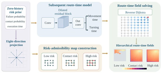
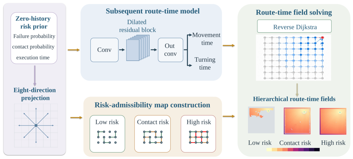
As shown in Figure 3, the fully convolutional subsequent route-time network uses a $3\times 3$ input convolution with 64 output channels, followed by six 64-channel residual blocks, each containing two $3\times 3$ convolutions, with block dilation rates $(1,1,2,4,1,1)$. A $1\times 1$ output convolution produces eight directional movement-time multipliers $M_h\left(u\right)$ and one turning-time gain $G\left(u\right)$. Both outputs are transformed by softplus, increased by 0.5, and clipped to $[0.5,20]$, ensuring positive time costs.

Figure 3. Subsequent route-time model and construction of hierarchical route-time fields.

For movement from cell u to adjacent cell v along direction h, edge execution time comprises movement and turning components:

$$\begin{array}{cc}\hfill t_{\mathrm{move}}(u,v,h)& ={\displaystyle \frac{\ell \left(h\right)\mathsf{\Delta }}{v_0}}{\displaystyle \frac{M_h\left(u\right)+M_h\left(v\right)}{2}},\hfill \\ \hfill t_{\mathrm{turn}}(u,p,h)& =k_{\mathrm{turn}}{\delta }_{\theta }(p,h)G\left(u\right),\hfill \\ \hfill t_{\mathrm{edge}}\left(e\right)& =t_{\mathrm{move}}(u,v,h)+t_{\mathrm{turn}}(u,p,h).\hfill \end{array}$$

Here, $\ell \left(h\right)\in \{1,\sqrt{2}\}$ corresponds to axial and diagonal movement, $v_0=0.8\mathrm{m}/\mathrm{s}$ is the base speed, and $k_{\mathrm{turn}}=0.18\mathrm{s}/\mathrm{rad}$ is the turning-time coefficient. Direction changes use the minimum angular distance between Heading8 directions, ${\delta }_{\theta }(p,h)={\displaystyle \frac{\pi }{4}}\min \left(\right|p-h|,8-|p-h\left|\right)$.

The risk class $\kappa \left(e\right)$ of directed edge e is determined by the standard-segment prediction at its source cell along the outgoing direction, using the thresholds in Section 2.4. Let ${\mathcal{E}}_{\mathrm{legal}}$ contain edges satisfying map-boundary and static hard-obstacle constraints with complete directional priors. The edge set for risk-admission level $\beta$ is

$${\mathcal{E}}_{\beta }=\{e\in {\mathcal{E}}_{\mathrm{legal}}:\kappa \left(e\right)⪯\beta \},\beta \in \{\mathrm{low},\mathrm{contact},\mathrm{high}\}.$$

The low-risk admission level admits only low-risk edges; the contact-risk admission level additionally admits contact-risk edges; and the high-risk admission level further admits high-risk edges, forming nested admissible edge sets.

The subsequent route-time model jointly learns movement and turning costs using the actual durations of successful trajectories along subsequent routes as supervision. The model learns turning costs from changes in local-goal commitment direction during training. During graph search, these costs are applied to direction changes between adjacent grid edges.

Movement and turning costs along a trajectory are summed to predict total duration, and training minimizes the mean squared error:

$$\begin{array}{cc}\hfill {\widehat{T}}_{\mathrm{route}}& ={\displaystyle \sum _{n=1}^{N_m}}{t}_{\mathrm{move}}\left(e_n\right)+{\displaystyle \sum _{n=1}^{N_t}}{t}_{\mathrm{turn}}\left(q_n\right),\hfill \\ \hfill {\mathcal{L}}_{\mathrm{RT}}& ={\displaystyle \frac{1}{N}}{\displaystyle \sum _{j=1}^N}{\left({\widehat{T}}_{\mathrm{route},j}-T_{\mathrm{route},j}\right)}^2.\hfill \end{array}$$

Here, $e_n,q_n$ denote movement and turning events, $N_m,N_t$ are their counts, N is the number of trajectories in the batch, and $T_{\mathrm{route},j}$ is the actual duration of trajectory j. Repeated events are counted each time they occur.

After training, the network generates goal-independent movement-time multipliers and turning gains, which are combined with directional risk priors to construct three risk-admission graphs. A reverse Dijkstra search is then run on each graph for a given goal. Let ${\mathcal{S}}_g$ contain the eight directional states of goal cell $u_g$. The remaining route time from state s at risk-admission level $\beta$ is

$$J_{\beta }(s,g)=\underset{\pi :s\to {\mathcal{S}}_g,\pi \subseteq {\mathcal{E}}_{\beta }}{\min }\sum _{e\in \pi }{t}_{\mathrm{edge}}\left(e\right).$$

States in the goal set have value zero; unreachable states have value $+\infty$.

The three risk-admission levels form a $3\times H\times W\times 8$ route-time field queried online by candidate cell and direction. Figure 3 shows its construction.

2.4. Candidate Local-Goal Generation and Selection Under Tiered Risk Constraints

At high-level decision step k, the system generates a set of candidate local goals ${\mathcal{E}}_k={\left\{e_{k,i}\right\}}_{i=1}^M$ spanning multiple directions and distances, converting continuous navigation space into a local decision space suitable for batched evaluation. Sources include regular angle–distance combinations, eight-direction sampling in world coordinates, task-goal ray sampling, short-range sampling along the task-goal direction, and the task goal when it enters candidate range. After map-boundary and model-input validity checks, candidates are aligned to common grid-cell centers and candidates sharing a cell are merged. When a task-goal candidate coincides with another candidate, the task-goal candidate is retained.

These five sources provide up to 203 raw candidate slots: 140 body-frame rule candidates (28 angles × 5 distances), 24 world-direction candidates (8 directions × 3 distances), 12 goal-ray samples, 26 short-range goal-relative candidates (13 angular offsets × 2 distances), and one terminal-goal candidate. Complete sampling parameters and validity rules are provided in Supplementary Section S3.1.

For brevity, write $e_i$ for $e_{k,i}$. The local execution model predicts arrival failure probability $P_{F,i}$, conditional non-foot contact probability $P_{D,i}$, and successful execution time ${\widehat{t}}_i$. Let $u_i$ be the candidate cell and $h_i$ the Heading8 direction corresponding to the world-frame direction from the robot to the candidate. Subsequent route time at risk-admission level $\beta$ is

$$J_{i,\beta }=J_{\beta }((u_i,h_i),g).$$

Current execution time represents the predicted local cost of reaching the candidate, while subsequent route time represents the candidate’s global route value. Both contribute to local-goal selection.

Current local-goal risk is divided into four classes according to arrival failure probability and conditional non-foot contact probability, with thresholds given in Table 2.

Table 2. Local execution risk classes and thresholds.

Risk Class	Condition
Low risk	$P_F\le 0.05$ and $P_D\le 0.20$
Contact risk	$P_F\le 0.05$ and $P_D>0.20$
High risk	$0.05<P_F\le 0.40$
Prohibited	$P_F>0.40$

The selector first retains candidate–admission combinations that satisfy input validity, current local-goal risk-class constraints, and subsequent route reachability. It then applies a strict-progress constraint. From the second commitment onward, the unadjusted remaining route time at risk-admission level $\beta$ must satisfy

$$J_{i,\beta }<J_{\mathrm{previous}}.$$

After each commitment, the selected candidate’s unadjusted remaining route time at the selected risk-admission level is stored as the reference for the next decision. This strict decrease suppresses repeated non-progressing choices while permitting temporary increases in straight-line distance to the goal during detours.

Eligible combinations are first filtered by current local-goal risk class, preferring candidates in the low-risk and contact-risk classes, and then by subsequent route risk-admission level, preferring low-risk and contact-risk admission levels. At each stage, admission is relaxed to the high-risk option only when the preferred set is empty. These two filtering stages produce the active combination set ${\mathsf{\Omega }}_k$; the candidates appearing in it form the active candidate set ${\mathcal{I}}_{\mathrm{active}}$.

A fixed surcharge is applied once if the current local goal belongs to the contact-risk class or the subsequent route uses the contact-risk admission level. Let $D_i^{\mathrm{cur}}$ and $D_{i,\beta }^{\mathrm{con}}$ indicate these two conditions, respectively. Then,

$$V_{i,\beta }=J_{i,\beta }+{\lambda }_D\mathbf{1}[D_i^{\mathrm{cur}}\vee D_{i,\beta }^{\mathrm{con}}],$$

Here, ${\lambda }_D=2.0\mathrm{s}$ is the contact-risk surcharge. For each active candidate, the risk-admission level ${\beta }_i^{*}$ minimizing $V_{i,\beta }$ is selected, and the total cost includes current execution time. The task-goal candidate is committed directly when the goal-priority conditions hold; otherwise, the local goal with the lowest total cost is selected:

$$Q_i={\widehat{t}}_i+V_{i,{\beta }_i^{*}},i^{*}=\arg \underset{i\in {\mathcal{I}}_{\mathrm{active}}}{\min }{Q}_i.$$

Algorithm 1 details the selection procedure and goal-priority conditions.

Algorithm 1 Local-goal candidate selection under tiered risk constraints.
Input: Candidate set ${\mathcal{E}}_k={\left\{e_i\right\}}_{i=1}^M$ with validity and task-goal flags; local execution predictions $P_{F,i}$, $P_{D,i}$, and ${\widehat{t}}_i$; remaining route time $J_{i,\beta }$ at three risk-admission levels; previous committed remaining route time $J_{\mathrm{previous}}$; contact-risk surcharge ${\lambda }_D$; and planar robot-to-goal distance $d_g$. Set $J_{\mathrm{previous}}=+\infty$ for the first commitment.
Output: Selected candidate $e_{i^{*}}$ and subsequent route risk-admission level ${\beta }_{i^{*}}^{*}$, or no eligible candidate.
	// Stage 1: Enforce current-execution and subsequent route constraints
1:	Initialize eligible combinations ${\mathcal{S}}_{\mathrm{valid}}\leftarrow ⌀$;
2:	for each candidate $e_i$:
3:	if inputs are invalid, ${\widehat{t}}_i$ is nonfinite, or $P_{F,i}>0.40$, skip this candidate;
4:	Determine the current local-goal risk class using the thresholds in Table 2;
5:	for each subsequent route risk-admission level $\beta$:
6:	if $J_{i,\beta }$ is finite, ($e_i$ is the task-goal candidate or $J_{i,\beta }>{10}^{-6}\mathrm{s}$), and $J_{i,\beta }<J_{\mathrm{previous}}$, add $(i,\beta )$ to ${\mathcal{S}}_{\mathrm{valid}}$;
7:	if ${\mathcal{S}}_{\mathrm{valid}}$ is empty, return no eligible candidate;
	// Stage 2: Prefer low-risk or contact-risk current local goals
8:	if ${\mathcal{S}}_{\mathrm{valid}}$ contains low-risk or contact-risk current candidates:
9:	${\mathcal{S}}_{\mathrm{current}}\leftarrow$ combinations belonging to those candidates;
10:	else ${\mathcal{S}}_{\mathrm{current}}\leftarrow$ combinations belonging to high-risk candidates;
	// Stage 3: Prefer low-risk or contact-risk subsequent route admission
11:	if ${\mathcal{S}}_{\mathrm{current}}$ contains low-risk or contact-risk admission levels:
12:	${\mathsf{\Omega }}_k\leftarrow$ combinations at those admission levels;
13:	else ${\mathsf{\Omega }}_k\leftarrow$ combinations at the high-risk admission level;
	// Stage 4: Compute costs and select an admission level per candidate
14:	for each active combination $(i,\beta )$, compute $V_{i,\beta }=J_{i,\beta }+{\lambda }_D\mathbf{1}[D_i^{\mathrm{cur}}\vee D_{i,\beta }^{\mathrm{con}}]$;
15:	for each candidate $e_i$ appearing in ${\mathsf{\Omega }}_k$:
16:	Select admission level ${\beta }_i^{*}$ minimizing $V_{i,\beta }$ and compute $Q_i={\widehat{t}}_i+V_{i,{\beta }_i^{*}}$;
	// Stage 5: Apply task-goal priority and select the final candidate
17:	if an active task-goal candidate exists and belongs to the low-risk class when $d_g>2.0\mathrm{m}$, or satisfies $P_{F,i}\le 0.40$ when $d_g\le 2.0\mathrm{m}$, return that candidate and its admission level;
18:	otherwise, minimize $Q_i$ over all active candidates, including the task-goal candidate; break total-cost ties using the fixed candidate order;
19:	return$(e_{i^{*}},{\beta }_{i^{*}}^{*})$.

Current local-goal risk represents the execution risk of reaching the candidate position, while subsequent route risk requires that a path from that position to the task goal satisfies the corresponding admission conditions on every directional edge. The deterministic selector combines these two risk assessments to select the local goal, thereby accounting for both current-segment executability and downstream terrain and reducing the likelihood of entering difficult-to-traverse regions. The goal is fixed in world coordinates for closed-loop tracking by the residual local planner and low-level controller. After each arrival within the handoff radius, the system regenerates candidates and evaluates subsequent routes from the actual position and heading, incorporating execution deviations into the next decision so that local execution outcomes continuously inform subsequent route decisions.

2.5. Residual Local Planning

After the upstream selector commits a local goal, residual local planning applies bounded corrections to a deterministic reference velocity command using real-time motion state, relative goal position, and local terrain. The deterministic reference provides goal alignment, forward motion, and deceleration during turns; the residual policy adjusts direction, speed, and yaw to accommodate nearby obstacles and terrain variations. The local goal remains fixed during execution, and a fixed-parameter low-level controller executes the corrected body-frame velocity commands. The configuration without residual planning directly uses the deterministic reference’s output.

Let $\theta$ be the local goal’s body-frame bearing and $v_0=0.8\mathrm{m}/\mathrm{s}$ the base speed. The base tracking commands are

$$\begin{array}{cc}\hfill v_x^{\mathrm{ref}}& =v_0\exp \left[-{\displaystyle \frac{1}{2}}{\left({\displaystyle \frac{\theta }{\sigma }}\right)}^2\right],\hfill \\ \hfill v_y^{\mathrm{ref}}& =(0.05\mathrm{m}/\mathrm{s})clip(d_y,-0.15,0.15),\hfill \\ \hfill {\omega }_z^{\mathrm{ref}}& =clip(k_{\omega }\theta ,-{\omega }_{\max },{\omega }_{\max }).\hfill \end{array}$$

Here, $d_y$ is the body-frame lateral component of the normalized goal direction, and clip denotes interval clipping. The parameters $\sigma =0.82\mathrm{rad}$, $k_{\omega }=1.8{\mathrm{s}}^{-1}$, and ${\omega }_{\max }=1.5\mathrm{rad}/\mathrm{s}$ are the heading-gate width, yaw gain, and yaw-rate limit, respectively.

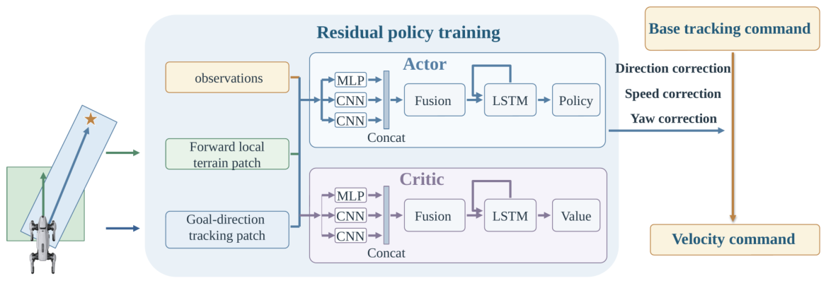
The residual policy observes 23 state and goal features, a forward local terrain patch, and a goal-direction tracking patch. Table 3 lists their contents and shapes. Both terrain inputs contain four channels: relative height, longitudinal slope, lateral slope, and local unevenness. Relative height uses ground elevation at the robot’s current position as its reference; slopes are computed from elevation differences on the respective sampling grids, and local unevenness is computed from neighborhood elevation deviations. All channels are normalized before network input.

Table 3. Residual policy observations.

Observation	Shape	Content and Coverage
State and goal	$\left[23\right]$	Body linear and angular velocities and projected gravity; relative goal position, normalized distance, and direction sine and cosine; previous bounded residual action, base tracking commands, and previous corrected velocity commands
Forward local patch	$[4,33,25]$	Aligned with the robot heading, covering a near-field region of approximately $4.8\mathrm{m}\times 3.2\mathrm{m}$
Goal-direction tracking patch	$[4,49,11]$	Along the committed local-goal direction, with maximum length $7.2\mathrm{m}$ and width approximately $1.6\mathrm{m}$

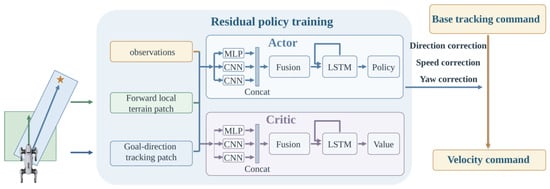
The policy and value networks use separate encoders: a $23\to 96\to 64$ MLP for state and goal features, and two terrain CNNs with channel widths $(32,48,64)$, each producing 96-dimensional features. The concatenated 256-dimensional feature passes through a $256\to 256\to 128$ fusion MLP and a single-layer LSTM with hidden size 128. The policy and value heads have hidden widths $(256,256,128)$ and output dimensions 3 and 1, respectively. Policy outputs are bounded by tanh to $a=(a_1,a_2,a_3)\in {[-1,1]}^3$, controlling direction, speed, and yaw corrections (Figure 4).

Figure 4. Network architecture and velocity-command generation for residual local planning.

Direction action $a_1$ adjusts the goal direction, and speed action $a_2$ scales the base command speed:

$$\begin{array}{cc}\hfill \delta \theta & =clip\left(\theta +a_1\delta {\theta }_{\max },-{\theta }_{\mathrm{fan}},{\theta }_{\mathrm{fan}}\right)-\theta ,\hfill \\ \hfill s& =1-(1-s_{\min })\max (-a_2,0).\hfill \end{array}$$

Here, $\delta {\theta }_{\max }=\pi /4\mathrm{rad}$ is the maximum requested direction correction. The half-angle of the permitted directional sector, ${\theta }_{\mathrm{fan}}$, is $\pi /2\mathrm{rad}$ during training and $\pi /3\mathrm{rad}$ during online navigation. The minimum speed ratio is $s_{\min }=0.25$, so planar speed magnitude is maintained or reduced relative to the base commands.

Planar velocity is obtained by rotating and scaling the base commands, while yaw rate includes the direction correction and the increment specified by action $a_3$:

$$\begin{array}{cc}\hfill \left[\begin{array}{c}{v}_x\\ v_y\end{array}\right]& =s\left[\begin{array}{cc}\cos \delta \theta & -\sin \delta \theta \\ \sin \delta \theta & \cos \delta \theta \end{array}\right]\left[\begin{array}{c}{v}_x^{\mathrm{ref}}\\ v_y^{\mathrm{ref}}\end{array}\right],\hfill \\ \hfill {\omega }_z& =clip\left({\omega }_z^{\mathrm{ref}}+k_{\omega }\delta \theta +\mathsf{\Delta }{\omega }_{\max }{a}_3,-{\omega }_{\max },{\omega }_{\max }\right).\hfill \end{array}$$

Here, $\mathsf{\Delta }{\omega }_{\max }=0.75\mathrm{rad}/\mathrm{s}$ is the yaw-rate increment limit; $k_{\omega }$ and ${\omega }_{\max }$ retain the deterministic reference’s values. Lateral velocity is finally clipped to $[-0.60,0.60]\mathrm{m}/\mathrm{s}$. Velocity commands are set to zero upon local-goal arrival or when the goal state is invalid.

The residual policy is trained using recurrent PPO. The per-step reward combines four categories of weighted signals: goal progress and arrival rewards encourage task completion; terrain clearance, non-foot contact, and failure penalties constrain execution risk; penalties on action magnitude and on changes in actions and velocity commands improve motion smoothness; and a per-step time cost promotes execution efficiency. Section 3.3 describes the training tasks. Complete reward definitions and the corresponding weights for both controllers are provided in Supplementary Table S6.

2.6. Model Training and Offline Precomputation

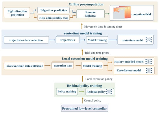
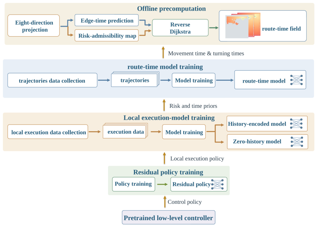
The system is trained sequentially, following the dependencies from low-level execution to high-level evaluation. With the pretrained low-level controller fixed, the residual local planning policy is trained first. The residual policy is then frozen, and closed-loop data are collected to train the local execution model. Next, map-wide directional priors are generated, successful trajectories along subsequent routes are collected to train the subsequent route-time model, and route-time fields are constructed. This process progressively incorporates controller-specific execution experience into high-level route evaluation, as shown in Figure 5.

Figure 5. Model-training dependencies and offline precomputation workflow.

The frozen residual policy and fixed low-level controller form the local-goal executor for data collection and online navigation.

Closed-loop local-goal execution data are collected from actual motion states and grouped by trajectory into training, validation, and test sets. History-encoded and zero-history models are trained separately. Monotonic Platt calibration uses all validation records for arrival failure probability and successful-arrival records for conditional non-foot contact probability, with calibration parameters folded into the output heads. The calibrated probabilities serve online candidate evaluation and map-wide directional projection; the zero-history model generates risk and time priors for standard motion segments along eight directions across the map.

Starting from actual handoff states, successive local goals are selected using risk and time priors and executed to collect closed-loop trajectories to the task goal. Given elevation and directional execution priors, the subsequent route-time model is then trained on the actual durations of successful trajectories along subsequent routes to learn movement-time multipliers and turning gains.

The subsequent route-time model generates map-wide edge-time parameters, which are combined with directional risk priors to construct three risk-admission graphs. Reverse Dijkstra search for a specified goal then produces route-time fields for online candidate evaluation.

When the map, execution configuration, and controller-specific models remain unchanged and only the task goal changes, directional priors and edge-time parameters can be reused, with only the route-time fields recomputed. Replacing the low-level controller requires training a corresponding residual policy, recollecting closed-loop data, retraining the local execution and subsequent route-time models, and regenerating the fields. When only the local execution policy changes, the subsequent workflow is repeated from closed-loop data collection onward. Section 3.3 provides training scales and parameters.

3. Experimental Setup

3.1. Simulation Platform and Controllers

Experiments use Isaac Lab and a Unitree Go2 model with terrestrial gravity of $9.81\mathrm{m}/{\mathrm{s}}^2$ and rigid contact. The physics time step is 0.005 s, and the navigation control period is 0.1 s. Each task runs for at most 600 navigation control steps, corresponding to 60 s.

The navigation base speed is $0.8\mathrm{m}/\mathrm{s}$, the maximum candidate local-goal distance is 7.2 m, and each local goal has an execution limit of 140 control steps (14 s). The handoff and task-goal arrival radii are both 0.35 m. Two pretrained low-level controllers, denoted A and B, are evaluated. Their inputs and network configurations are summarized in Table 4.

Table 4. Low-level controller configurations.

Controller	Input Dimension	Policy Network	Main Inputs
A	45	$45\to 512\to 256\to 128\to 12$	Velocity commands, proprioceptive state, and joint state
B	235	$235\to 512\to 256\to 128\to 12$	Velocity commands, proprioceptive state, joint state, and height scans

The controller-specific models are trained and generated using the workflow in Section 2.6.

The low-level controllers are externally pretrained. The residual policy is trained for 2000 iterations and requires approximately 7.6 h. Data collection, training, field generation, and system evaluation for the risk and route-time models together require approximately 6.7 h, of which model training accounts for approximately 32 min. Online navigation decisions take 40.98 ms on average. Detailed training, timing, and resource-use results are provided in Supplementary Section S3.4.

3.2. Complex Unstructured Terrain and Tasks

The evaluation set contains 36 unstructured-terrain maps, each with one fixed start and task goal, giving 36 navigation tasks. Each map covers 24 m × 24 m at 0.1 m grid resolution. A procedural generator superimposes slopes, craters, ridges, basins, rocks, and rubble on a continuously undulating base elevation field, with passages, exits, and alternative routes designed relative to robot size.

The geometry and start–goal pairs of these 36 maps were fixed before evaluation. All three evaluation seeds use the same maps and tasks; their scope is explained in Section 3.4. Straight-line start–goal distances range from 9.83 to 22.09 m, and geometric reference-route lengths from 12.76 to 33.79 m, covering direct traversal, local detours, and global route alternatives.

To assess transfer to an unseen layout, one independent map not used in training was selected, and 12 navigation tasks were defined from terrain geometry. All models and planning parameters remained fixed, and the same control and termination settings as in the main evaluation were used; each task was run once with seeds 1, 42, and 43. The map, task definitions, and complete configuration are provided in Supplementary Section S2.

Online planning uses finite-resolution grid elevation maps converted from the physical height fields, representing prior maps with regional coverage and limited spatial accuracy. Planning models obtain terrain information only through these elevation maps. Physics-engine contact information is used solely to generate training labels and determine execution outcomes. Table 5 summarizes terrain classes, principal generation scales, and navigation challenges.

Table 5. Evaluation terrain classes and navigation challenges.

Terrain Class	Tasks	Main Generation Scales	Navigation Challenge
Open rough terrain	4	Base undulation amplitude $0.12$–$0.35\mathrm{m}$; 7–18 local bumps	Heading stability and speed maintenance
Crater detours	5	Crater radius $1.91$–$3.60\mathrm{m}$, depth $0.22$–$1.16\mathrm{m}$, rim height $0.11$–$0.52\mathrm{m}$	Short-route risk versus long-route cost
Ridge–saddle crossings	3	Ridge height $0.57$–$0.77\mathrm{m}$; saddle width $3.44$–$4.12\mathrm{m}$	Entry selection and cross-slope traversal
Rubble gaps	4	19–40 main rubble elements, radius $0.44$–$0.54\mathrm{m}$; elevation perturbation $0.10$–$0.15\mathrm{m}$	Traversability at robot scale
Rock-cluster detours	2	18 rocks per map, radius $0.54$–$1.02\mathrm{m}$	Successive local-goal selection
Narrow passage	1	Passage width $1.45\mathrm{m}$; side-obstacle height $0.65\mathrm{m}$	Candidate precision and local tracking
Mixed macro routes	4	Mountain height approximately $1.40\mathrm{m}$, basin depth approximately $1.06\mathrm{m}$, traversable-band width approximately $1.83\mathrm{m}$	Sustained progress across terrain regions
Moderate-risk crossings	2	190–280 rubble elements; one map additionally has a ${28}^{\circ }$ slope	Risk eligibility and relaxed admission
Basin rims	2	Elliptical semiaxes $5.4\mathrm{m}$ and $4.4\mathrm{m}$; depth $0.46\mathrm{m}$	Rim-following routes and exit selection
Macro-cone routes	3	Radius $7.20$–$7.45\mathrm{m}$, peak height $2.88$–$3.03\mathrm{m}$, side slope approximately $21.8^{\circ }$–$22.8^{\circ }$	Global detour evaluation
Mountain switchbacks	2	Ascent height $1.28\mathrm{m}$; switchback-band width $3.2\mathrm{m}$	Turning cost and route continuity
Annular-crater routes	2	Inner and outer radii $0.70\mathrm{m}$ and $5.25\mathrm{m}$; depth $1.52\mathrm{m}$	Detours under tiered risk constraints
Multi-crater forced routes	2	Elliptical crater semiaxes $1.05$–$3.25\mathrm{m}$; depth $0.46$–$1.31\mathrm{m}$	Successive exit choices among craters
Total	36	—	—

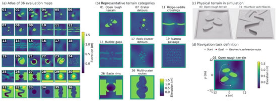
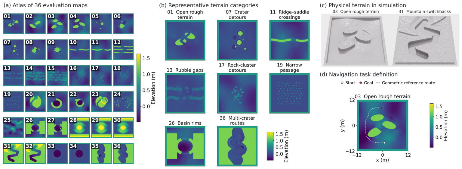
The terrain set is constructed from geometric types relevant to lunar surface exploration, with constrained passages and alternative routes added to test navigation in complex unstructured environments [3,28]. The parameters in the table are design values for the simulation benchmark and define geometric challenges relevant to lunar surface exploration. They are not calibrated to measured lunar south-polar elevation statistics. Figure 6 shows representative terrains and tasks.

Figure 6. Evaluation terrains and navigation-task examples. (a) Overview of the 36 evaluation maps; (b) representative terrain classes; (c) examples of physical simulation terrains; and (d) navigation-task examples, where white dots, red stars, and white dashed lines indicate starts, goals, and geometric reference routes, respectively.

3.3. Training Tasks, Data Collection, and Controller-Specific Models

Training data for the local execution and subsequent route-time models are primarily collected on 216 physical variants of the 36 base maps, covering baseline, flat, rough, slope, edge, and mixed settings. Physical terrain sampling is 0.05 m, while the original 0.1 m navigation maps are retained. All perturbed variants include smoothed flat-region noise with a standard-deviation scale of 0.006 m. Slope perturbations use a 0.35 m smoothing scale and a 0.026 m standard-deviation scale, clipped to ± 0.045 m. Rough-region perturbations include Gaussian bumps with radii of 0.055–0.18 m and heights of 0.055–0.16 m. Edge perturbations use a 0.055 m noise standard-deviation scale, clipped to [−0.07, 0.09] m. Components act within eligible terrain regions, preserving protected and hard-obstacle cells; mixed variants combine the components. The local execution model additionally uses closed-loop records from the base terrain set. Detailed terrain perturbation methods, parameter settings, and the correspondence between terrain variants and training tasks are provided in Supplementary Section S3.3.

The residual policy is trained for local-goal tracking with a fixed low-level controller. Tasks cover straight motion and turning, local obstacle avoidance, slope traversal, and tracking over irregular terrain. The training set includes 29 local terrain classes and 2784 fixed goals, with distances of $1.5$–$7.0\mathrm{m}$ and relative bearings of $[-{60}^{\circ },{60}^{\circ }]$. Training uses random seed 42 and at most 140 navigation control steps per episode.

Local execution data collection, trajectory-group splitting, and probability calibration follow Section 2.6.

Subsequent route data are collected using strata defined by entry local-goal distance and direction. Entry distance is the robot-to-local-goal distance before commitment, divided into 1–$2.5\mathrm{m}$, $2.5$–$5\mathrm{m}$, and 5–$7.2\mathrm{m}$ intervals, with all eight Heading8 world directions covered. The actual handoff state after completing the entry commitment becomes the subsequent route trajectory’s starting state. Table 6 reports dataset sizes and splits for both controllers, using the configuration IDs in Section 3.4.

Table 6. Controller-specific dataset sizes and splits.

Configuration	Local Records/Trajectories	Local Execution Train/Val./Test	Successful Subsequent Routes	Subsequent Route Train/Val./Test
A + residual (001)	47,520/24,196	38,070/4770/4680	9830	7790/1076/964
B + residual (008)	47,520/24,908	37,928/4811/4781	8639	6884/918/837

Table 7 summarizes the main training hyperparameters used with controllers A and B. Route-time fields are generated after training as described in Section 2.6. Complete network and training configurations are provided in Supplementary Section S3.2.

Table 7. Main training hyperparameters.

Module	Training Setup	Main Hyperparameters
Local execution model	AdamW; maximum 40 epochs; batch size 256	Learning rate $3\times {10}^{-4}$; weight decay ${10}^{-4}$; validation-loss checkpoint selection; early-stopping patience 8 epochs, with a minimum of 12 epochs
Subsequent route-time model	AdamW; 80 epochs; batch size 16 trajectories	Learning rate $3\times {10}^{-5}$; weight decay ${10}^{-5}$; 1 warm-up epoch
Residual policy	Recurrent PPO with Adam; 1536 environments; 24 rollout steps per environment; 2000 iterations	Fixed learning rate $2\times {10}^{-4}$; 4 learning epochs and 6 minibatches per iteration; discount 0.99; GAE 0.95; clipping 0.2; entropy coefficient 0.004; maximum gradient norm 1.0

3.4. Comparisons, Module Ablations, and Evaluation Metrics

Eight system configurations are evaluated, as listed in Table 8. The complete configuration using controller A and residual local planning is denoted 001. Configurations 002–006 ablate local execution-risk prediction, subsequent route evaluation, and tiered risk-constrained selection. Configurations 007 and 008 compare complete systems without residual execution and with a different low-level controller, respectively.

Table 8. Internal comparison configurations.

ID	Controller/Local Execution	Current Local-Goal Risk	Subsequent Route Evaluation	Selection	Comparison
001	A + residual	Full learned risk	Learned	Tiered risk	Full method
002	A + residual	Risk neutralized	Learned	Tiered risk	Current-risk ablation
003	A + residual	Full learned risk	Geometry-only subsequent route	Tiered risk	Subsequent route ablation
004	A + residual	Full learned risk	Constant-velocity subsequent route	Tiered risk	Subsequent route ablation
005	A + residual	Full learned risk	Myopic; no strict progress	Tiered risk	Subsequent route ablation
006	A + residual	Full learned risk	Learned	Flat cost	Selection ablation
007	A, no residual	Full learned risk; retrained	Learned; retrained	Tiered risk	Full-system comparison
008	B + residual	Full learned risk; retrained	Learned; retrained	Tiered risk	Full-system comparison

All configurations use zero-history local execution models for online candidate evaluation. The map-wide directional priors needed for learned subsequent route evaluation are also generated by the corresponding zero-history model.

Configurations 002–006 modify configuration 001 as follows.

Configuration 002 sets the current-candidate arrival failure probability and conditional non-foot contact probability to zero while retaining the candidate set, current execution-time prediction, and subsequent route evaluation.

Configurations 003 and 004 use the same directed eight-neighbor grid graph, retaining map-boundary checks, hard-obstacle checks over the body swept area, and directional height-difference constraints. Configuration 003 weights edge length by clearance weight $w=1+0.35c_{\mathrm{clearance}}$, where $c_{\mathrm{clearance}}$ increases near hard-obstacle regions; configuration 004 uses edge length directly. Both compute the minimum accumulated cost through reverse Dijkstra search and divide it by the base speed to obtain subsequent route time. All three risk-admission levels share this query value. Both configurations retain learned risk and time predictions for current local goals, risk-class and risk-admission filtering, and strict progress.

Configuration 005 removes subsequent route-cost evaluation and the strict-progress constraint, selecting solely from current local-goal risk and execution time.

Configuration 006 retains risk predictions and route-time fields but removes risk-class and risk-admission priority and the contact-risk surcharge, allowing for all eligible candidates to compete directly on total execution time.

Configuration 007 disables residual local planning, then recollects data, retrains the local execution and subsequent route-time models, and regenerates fields for that execution mode. Configuration 008 uses controller B, retrains all controller-specific learned modules, and regenerates the fields according to Section 2.6.

External comparisons use ArtPlanner-geometric (hereafter ArtPlanner-G) and X-NavDP. ArtPlanner-G retains the sampling-based planning core and constructs routes using the global elevation map, foot-support margin, and permissible drop height [29]. X-NavDP retains diffusion-based trajectory generation, trajectory-value evaluation, historical-trajectory guidance, and model predictive control. To adapt the method to the platform, low-level controller, and terrain used in this study, its reinforcement-learning post-training uses 612 tasks associated with the 36 evaluation maps, comprising the 36 evaluation tasks and 576 same-map variants. Its online inputs include forward local RGB-D with an effective range of $5\mathrm{m}$, a body-frame goal vector, robot pose, and historical local trajectories [25].

The proposed method and ArtPlanner-G use the global elevation map, while X-NavDP uses forward local RGB-D with an effective range of $5\mathrm{m}$. The three sets of results therefore describe complete navigation-system performance under their respective observation conditions.

The proposed method in the external comparison uses configuration 001. The three methods use the same 36 tasks and evaluation seeds 1, 42, and 43, together with low-level controller A, a maximum linear speed of $0.8\mathrm{m}/\mathrm{s}$, single-environment execution, and a 600-control-step limit.

Each run initializes the environment and relevant random-number states using its assigned seed. Maps, task order, starts, initial headings, goals, initial joint states, and physical parameters remain identical. Observation noise or stochastic sampling is applied according to each method’s evaluation configuration. Configuration 001 uses fixed tasks, deterministic candidate selection, and deterministic policy inference; its three-seed runs test repeatability under this evaluation setup. The 36 fixed tasks and three seeds yield 108 evaluation episodes.

Navigation performance is evaluated by success rate and termination type. Success rate is the proportion of successful episodes among all evaluation episodes. Termination types include body contact, posture anomaly, stuck, timeout, no valid candidate, and other non-arrival outcomes. No valid candidate means that the next selection produces no eligible candidate after local-goal arrival. Execution efficiency is evaluated using mean control steps on paired jointly successful episodes, together with local-goal commitment counts and commitment distances. Paired episodes share the same task and evaluation seed. The mean number of control steps over all episodes describes overall run length and is influenced by both early failures and timeouts.

The probability predictions of the local execution model are evaluated using the Brier score and expected calibration error:

$$\begin{array}{cc}\hfill BS& ={\displaystyle \frac{1}{N}}{\displaystyle \sum _{n=1}^N}{(p_n-y_n)}^2,\hfill \\ \hfill {ECE}_{10}& ={\displaystyle \sum _{k=1}^{10}}{\displaystyle \frac{|B_k|}{N}}\left|freq\left(B_k\right)-conf\left(B_k\right)\right|.\hfill \end{array}$$

Here, $p_n$ is the predicted probability, $y_n$ the binary label, and N the number of relevant test records. ECE divides $[0,1]$ into ten equal-width bins. $B_k$ is the sample set in bin k; $freq\left(B_k\right)$ and $conf\left(B_k\right)$ are its observed event frequency and mean predicted probability. Empty bins contribute zero. Arrival failure probability is evaluated on all test records, while conditional non-foot contact probability is evaluated only on successful-arrival records.

For reference, using the observed event proportion $\overline{y}$ in the relevant test records as a constant probability prediction yields a Brier score of $\overline{y}(1-\overline{y})$. Local successful execution time is evaluated by mean absolute error (MAE). Subsequent route time is evaluated by MAE, mean squared error (MSE), and mean bias. Relative MAE is MAE divided by mean actual time, and mean bias is the mean predicted time minus actual time.

4. Results and Discussion

4.1. Overall Results

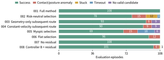
Table 9 summarizes task completion and mean control steps over all episodes for the eight configurations. The proposed method (001) and the complete configuration without residual planning (007) both achieve a task success rate of 100% across 108 evaluation episodes. All five module-ablation configurations show reduced success rates, with the largest decline in the myopic configuration 005.

Table 9. Task completion and mean control steps by configuration.

ID	Configuration	Seed 1	Seed 42	Seed 43	Total Successes	Success Rate	Mean Steps, All Episodes
001	Proposed method	36/36	36/36	36/36	108/108	100.00%	293.33
002	Risk-neutral selection	26/36	26/36	26/36	78/108	72.22%	259.94
003	Geometry-only subsequent route	31/36	31/36	31/36	93/108	86.11%	272.14
004	Constant-velocity subsequent route	30/36	30/36	30/36	90/108	83.33%	275.36
005	Myopic selection	23/36	23/36	23/36	69/108	63.89%	433.17
006	Flat selection	32/36	32/36	32/36	96/108	88.89%	265.67
007	No residual	36/36	36/36	36/36	108/108	100.00%	296.72
008	Controller B + residual	34/36	34/36	33/36	101/108	93.52%	260.52

Note: Results aggregate 108 episodes from 36 fixed tasks and three evaluation seeds. The mean number of control steps over all episodes includes successes and failures and describes overall run length.

Configurations using controller A produce identical task-level outcomes across the three evaluation seeds. The complete configuration with controller B and residual planning succeeds in 34, 34, and 33 tasks on the three seeds, respectively. The proposed method succeeds in all 36 tasks in each run, demonstrating repeatable task completion on the current fixed evaluation set.

Figure 7 shows the distribution of successes and termination types for each configuration.

Figure 7. Task outcomes by configuration. Each configuration includes 108 evaluation episodes; numbers indicate outcome counts. Termination categories are mutually exclusive, with contact and posture anomaly combined.

On the independent map, the proposed method completed 11 of the 12 tasks with each seed, yielding 33/36 (91.67%). All three failures occurred on the same pit-exit task, where the robot did not reach the goal within the time limit. Full results and failure analysis are provided in Supplementary Section S2.

4.2. External Baseline Comparisons

Table 10 compares task completion for the proposed method, ArtPlanner-G, and X-NavDP under the evaluation conditions in Section 3.4.

Table 10. Task completion for external baseline comparisons.

Method	Successful Episodes	Mean Steps, Successful Episodes
Proposed method	108/108 (100.00%)	293.33
ArtPlanner-G	98/108 (90.74%)	300.55
X-NavDP	84/108 (77.78%)	377.01

Table 11 compares mean control steps on paired jointly successful episodes, including only episodes in which both methods succeed for the same task and evaluation seed.

Table 11. Execution efficiency on paired jointly successful episodes in external comparisons.

Baseline	Jointly Successful Episodes	Proposed Method Mean Steps	Baseline Mean Steps	Baseline Increase
ArtPlanner-G	98	292.72	300.55	7.83
X-NavDP	84	280.88	377.01	96.13

ArtPlanner-G succeeds in 98 of 108 evaluation episodes, with nine body-contact failures and one non-arrival. It primarily optimizes geometric route length. Fixed parameters such as foot-support margin and permissible drop height define explicit geometric traversability conditions, but they provide limited representation of the low-level controller’s actual capability on terrain near its execution limits and of the spatial margin needed for posture changes and tracking errors. The recorded trajectories show that ArtPlanner-G tends to select shorter routes, often passing close to crater rims or rock boundaries without sufficient safety margins; failures typically occur near the controller’s capability limits. Mean control steps on jointly successful episodes are similar for the two methods, while the proposed method achieves a higher success rate. This suggests that combining closed-loop execution prediction with subsequent route-risk constraints helps assess execution risk near capability limits and preserve larger safety margins.

X-NavDP succeeds in 84 of 108 evaluation episodes. It generates short-range trajectories from forward local RGB-D, whose limited observation range cannot capture the full structure of distant detours. The recorded trajectories show repeated direction changes, long detours, or entry into longer branches in junction tasks, complex obstacle-avoidance tasks, and mountain-switchback tasks. When successive trajectory directions differ substantially, the model predictive controller also slows or briefly stops to replan. These behaviors correspond to longer completion times on jointly successful episodes.

When a global elevation map is available before execution, the proposed method selects local goals using global terrain structure and controller-specific risk and time evaluation. It achieves a higher task completion rate on the current evaluation set and, on jointly successful episodes, greater execution efficiency than X-NavDP.

4.3. Module Ablations and Parameter Sensitivity

For local execution-risk prediction, setting the current-candidate arrival failure probability and conditional non-foot contact probability to zero in configuration 002 reduces success to 72.22%, with additional failures including physical contact, stagnation, and timeout. With current execution-time prediction and subsequent route evaluation retained, these results indicate that current local-goal risk information helps identify candidates likely to cause physical failure or difficult local-goal completion, reducing ineffective progress caused by insufficient execution capability.

For subsequent route evaluation, configurations 001 and 003–005 are compared to assess how subsequent route evaluation affects local-goal selection and navigation outcomes. The clearance-weighted geometric configuration (003) and the constant-speed configuration (004) achieve success rates of 86.11% and 83.33%, respectively, both above the 63.89% achieved by the myopic configuration (005). These results indicate that retaining subsequent route evaluation and the strict-progress constraint improves global route guidance and sustained progress. However, their uniform geometric cost fields provide limited representation of controller-specific directional execution times and tiered risk-class and admission conditions, yielding lower completion rates than complete configuration 001.

The myopic configuration (005) removes both subsequent route-cost evaluation and strict progress. It reaches the time limit in multiple tasks, and some episodes incur body contact late in execution. Choosing goals solely from current local-goal risk and time can therefore lead to prolonged stagnation and ineffective progress. This configuration shows the largest degradation, indicating that using subsequent route cost to assess global route value, together with a decrease in remaining route time across successive commitments, helps distinguish downstream routes in advance, guide detours, and sustain progress.

For tiered risk-constrained selection, configuration 006 retains risk predictions and route-time fields while removing risk-class and risk-admission priority and the contact-risk surcharge. Success falls to 88.89%, and all additional failures involve body contact. When all eligible candidates compete directly on total execution time, shorter predicted durations can favor high-risk candidates. Prioritizing lower-risk current candidates and admission levels, together with the contact-risk surcharge, constrains selection and helps preserve execution-safety margins.

The ablations show complementary roles: local execution-risk prediction judges local-goal executability, subsequent route evaluation assesses candidates’ global route value, and tiered risk-constrained selection regulates competition among options with different risks. Together, they support local-goal selection that accounts for both execution safety and route efficiency.

Figure 7 shows overall termination-type composition by configuration; Supplementary Section S2 further lists failure rates and termination types for the eight internal configurations by terrain family.

With model parameters fixed, a one-factor sensitivity analysis was performed on the original 36 tasks and three evaluation seeds. Thresholds of 0.03 and 0.05 for low-risk arrival failure probability yielded 100% success, whereas a threshold of 0.08 reduced success to 97.22%. All groups maintained 100% success when the prohibited-risk threshold varied from 0.30 to 0.50 and the conditional non-foot contact threshold varied from 0.10 to 0.30. With contact surcharges of 0 and $1\mathrm{s}$, body-contact failures occurred, whereas surcharges of 2 and $3\mathrm{s}$ yielded 100% success; $3\mathrm{s}$ increased mean paired duration by $0.35\mathrm{s}$ relative to $2\mathrm{s}$. These results support the current threshold combination and indicate that a $2\mathrm{s}$ surcharge balances task completion and execution efficiency within the tested range. Complete results are provided in Supplementary Section S3.4.

4.4. Complete Configurations with and Without Residual Planning

This section compares residual configuration 001 with non-residual configuration 007. Each uses a local execution model and route-time fields corresponding to its execution mode, so the comparison reflects system-level differences between complete configurations. Both achieve 100% task success. Table 12 reports local-goal commitments and execution efficiency.

Table 12. Complete configurations with and without residual planning.

Configuration	Successes/Total	Mean Control Steps	Mean Local-Goal Commitments	Mean Ordinary Local-Goal Distance (m)
Residual	108/108	293.33	9.81	2.058
No residual	108/108	296.72	11.44	1.784

Note: Both configurations use controller A. Control steps and local-goal commitments are averaged over 108 evaluation episodes.

The non-residual configuration tracks the local goal by moving toward it and turning in place when the heading deviation is large. Terrain adaptation relies on high-level local-goal selection and the low-level controller’s locomotion capability. While the committed goal remains unchanged, the residual configuration continuously adjusts direction, speed, and yaw according to local terrain variations and obstacle distribution.

Relative to the non-residual configuration, the residual configuration increases the mean commitment distance for non-terminal local goals by 15.39%, reduces mean local-goal commitment count by 14.32%, and reduces mean control steps by 1.14%. These results indicate that the controller-specific risk and time models reflect changes in the local execution mode, enabling high-level planning to adjust the commitment scale according to the execution capability. A single commitment can cover a more distant local goal, allowing for the system to complete navigation with fewer high-level commitments and correspondingly fewer candidate-set reconstructions and risk–cost evaluations.

4.5. Performance with Different Low-Level Controllers

This section compares configuration 001 using controller A with configuration 008 using controller B, evaluating the prediction accuracy of the controller-specific models and overall navigation performance. Both use identical candidate definitions, risk labels, route-time definitions, selection rules, and navigation-layer hyperparameters. The controller-specific models are trained on the respective controller’s closed-loop data and evaluated on the same task set.

Table 13 reports probability predictions of the controller-specific local execution models.

Table 13. Local execution model probability predictions.

Controller	Event	Test Samples	Event Proportion	Brier	Constant-Baseline Brier	ECE
A	Arrival failure	4680	50.24%	0.03489	0.24999	0.00689
B	Arrival failure	4781	50.76%	0.04721	0.24994	0.00968
A	Conditional non-foot contact	2329	30.74%	0.10596	0.21292	0.02267
B	Conditional non-foot contact	2354	13.08%	0.06924	0.11372	0.01473

Note: Non-foot contact metrics are conditional on successful arrival. The constant baseline predicts the corresponding test-set event proportion $\overline{y}$, yielding a Brier score of $\overline{y}(1-\overline{y})$.

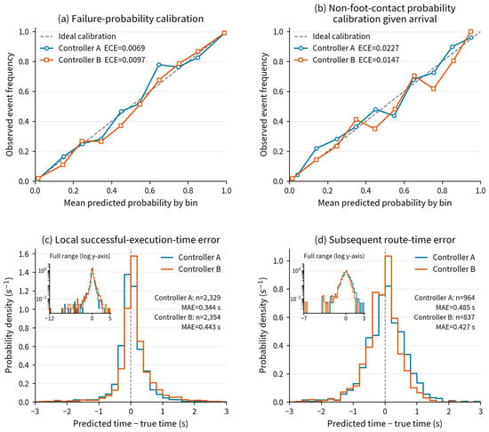
Both models have Brier scores below their corresponding constant baselines. The ECE values for arrival failure probability and conditional non-foot contact probability are below 0.01 and 0.023, respectively, indicating good probability prediction and calibration performance. Because the current local-goal risk class and subsequent route risk-admission level determine candidate eligibility and priority, underestimating execution risk can cause the selector to choose a candidate with higher actual risk even when a lower-risk feasible option exists, leading to contact, stagnation, or arrival failure.

Table 14 summarizes test results for both time models. Local successful execution-time MAE is below 0.45 s, with relative MAE below 8%. Subsequent route-time MAE is below 0.5 s, with relative MAE of approximately 3.4% and absolute mean bias below 0.1 s, indicating accurate time prediction for the data distribution of each controller. After stratification by the 13 terrain classes, the subsequent route-time relative MAE remains below 6% for both controllers. The highest values are 2.4% for controller A on the mountain-switchback class and 5.9% for controller B on the narrow-passage class; complete group statistics are provided in Supplementary Section S1.

Table 14. Local execution and subsequent route-time prediction results.

Prediction Task	Controller	Test Samples	Actual Time (s) Mean/Median	MAE (s)/Relative MAE (%)	MSE (s2)	Mean Bias (s)
Local execution	A	2329	5.903/5.700	0.344/5.83	—	—
Local execution	B	2354	5.585/5.300	0.443/7.92	—	—
Subsequent route	A	964	13.978/13.000	0.4851/3.47	0.4614	+0.0242
Subsequent route	B	837	12.708/11.700	0.4267/3.36	0.4754	$-0.0992$

Note: Local execution time is evaluated on successful-arrival records; subsequent route time is evaluated on successful trajectories from actual handoff states to the task goal. Dashes indicate unreported metrics.

Figure 8 presents probability calibration curves and time-prediction error distributions for the controller-specific models.

Figure 8. Prediction accuracy of the controller-specific models. (a) Arrival failure probability calibration; (b) non-foot contact probability calibration conditional on successful arrival; (c) local successful execution-time error; and (d) subsequent route-time error. Results use each model’s independent test set. Dashed lines indicate ideal calibration. Time error is predicted minus actual time, and probability density is normalized over the full test sample set; insets show the full error range on a logarithmic vertical axis.

Among 108 evaluation episodes, the configurations using controllers A and B succeed in 108 and 101, respectively. Of controller B’s seven failures, six occur on two maps that require crossing a basin-rim step. The recorded trajectories show controller B approaching the step along the planned route and attempting to cross, then incurring body contact, abnormal orientation, or stagnation after unsuccessful traversal. Both maps lack a viable detour, so these failures are associated with controller B’s limited obstacle-crossing capability.

Across the 101 jointly successful episodes, mean control steps are 297.89 for controller A and 265.81 for controller B. Controller B requires 32.08 fewer control steps on average. The recorded trajectories show more pronounced foot lifting and body-posture adjustments for controller A, while controller B exhibits smaller posture changes.

4.6. Route Selection with Different Low-Level Controllers

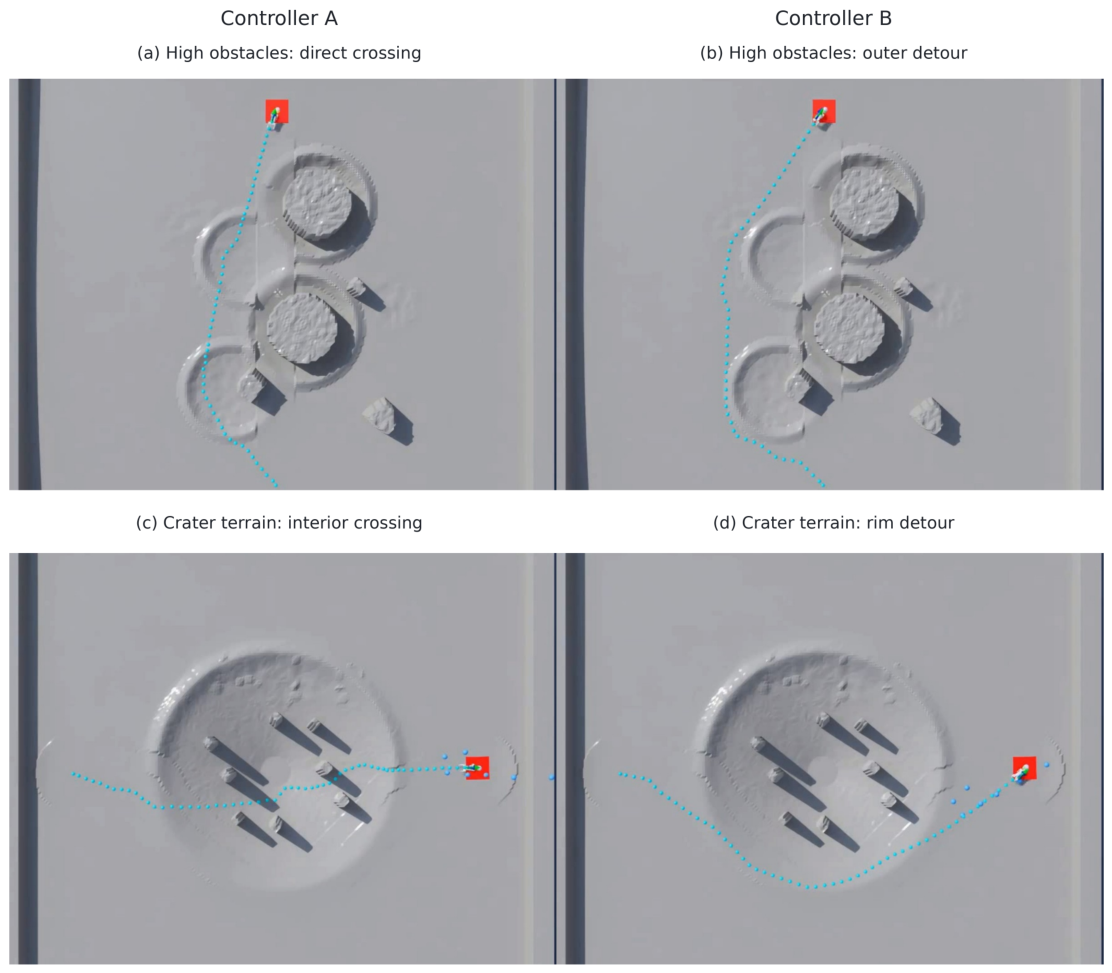
This section examines tasks on consecutive high-step and crater terrain to compare the outcomes of the two controller configurations and illustrate how differences in local execution capability affect route selection.

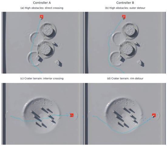
On the consecutive high-step terrain shown in Figure 9a,b, controller A crosses the obstacles directly, while controller B detours around the obstacle region. On the crater terrain shown in Figure 9c,d, controller A traverses depressions and obstacle gaps, while controller B follows the rims. Controller A takes a more direct route in both task types.

Figure 9. Route selection by different low-level controllers on two terrain types. The left and right columns correspond to controllers A and B, respectively; blue dots indicate robot trajectories. (a,b) Consecutive high-step terrain; (c,d) crater terrain.

The two configurations follow different detour and obstacle-crossing routes, consistent with the controller execution characteristics observed in the preceding section: controller A exhibits more pronounced foot lifting and body-posture adjustments and therefore more often selects obstacle-crossing routes that shorten travel distance; controller B exhibits smaller posture changes and limited obstacle-crossing ability and therefore tends to select routes around obstacle boundaries. These results show that, with the navigation-layer architecture and parameters held fixed, the proposed method learns execution risk and time from controller-specific closed-loop data, enabling global route selection to adapt to the local execution capabilities of different controllers.

4.7. Lunar Relevance, Limitations, and Future Work

The reduced gravity and regolith contact conditions on the Moon alter robot traversal capability and execution time. Experiments with two low-level controllers show that risk and time models learned from their respective closed-loop data enable route evaluation and selection to adapt to controller capability, providing a methodological basis for future adaptation to lunar motion controllers. Current experiments use terrestrial gravity and rigid contact. Further validation should incorporate real lunar elevations, reduced gravity, and deformable regolith, construct controller-specific models using Section 2.6, and assess prediction accuracy and closed-loop navigation through physical robot experiments.

The method requires a prior elevation map covering the task area and is suited to goal navigation near landers and within surveyed work areas. Surveying and localization errors affect planning in such settings: elevation errors can alter slope-break, edge, and local-support features, while localization and map-registration errors can misalign the terrain used for candidate evaluation with the actual execution position, affecting risk judgments and route-time estimates. Future evaluation will vary map resolution, elevation noise, and registration error to establish the method’s tolerance to practical mapping errors.

When the task goal lies beyond the mapped region, or when sampling missions require autonomous target search, the robot must choose exploration directions and update route evaluation as observations accumulate. Future work will integrate simultaneous localization and mapping (SLAM), allowing for the navigation system to jointly consider execution risk, route time, and information gain when choosing exploration directions. The local execution model and residual local planner can support candidate evaluation and closed-loop execution within observed regions. Subsequent route evaluation must adapt to map expansion and changing task goals, extending the system to autonomous exploration of unknown areas.

5. Conclusions

This paper presents hierarchical quadruped navigation based on risk and execution cost evaluation for future lunar missions, with simulation validation on unstructured terrain. Controller-specific closed-loop data are used to build local execution and subsequent route-time models, respectively evaluating the execution risk and execution time of reaching candidate local goals and the subsequent route time from candidate positions to the task goal. Subsequent route cost assesses each candidate’s global route value. The system selects local goals under tiered risk constraints and uses residual local planning for continuous tracking, transferring differences in local execution capability to global route selection.

Across 108 episodes comprising 36 unstructured-terrain tasks and three evaluation seeds, the proposed method using controller A and a zero-history local execution model succeeds in all episodes, while ArtPlanner-G and X-NavDP succeed in 98 and 84, respectively. Mean control steps on jointly successful episodes are similar for the proposed method and ArtPlanner-G, with a higher task completion rate for the proposed method. Both types of prediction models achieve low errors on their controller-specific test sets. Module ablations show that local execution-risk prediction, subsequent route evaluation, and tiered risk-constrained selection all contribute to task completion, with the largest degradation when subsequent route evaluation and strict progress are removed. On a map not used in training, the proposed method completes 33 of 36 episodes (91.67%), and all three failures occur on the same pit-exit task due to timeout.

Complete configurations with and without residual planning both achieve 100% success across 108 evaluation episodes. By continuously correcting motion direction, speed, and yaw, residual local planning enables more flexible obstacle avoidance and turning within a single local-goal tracking segment. With similar navigation durations, it reduces mean local-goal commitment count by 14.32%, lowering high-level decision frequency. The configuration using controller B achieves 93.52% task success. The two controller configurations produce different detour and obstacle-crossing routes on identical maps, demonstrating that controller-specific risk and time models convey local execution-capability differences to global route selection.

The method targets autonomous navigation with a regional elevation map. Current results validate the navigation layer under terrestrial gravity and rigid-contact simulation. Future work will evaluate map-error effects and investigate navigation and autonomous exploration as maps expand. Physical robot validation will also incorporate real lunar terrain data in experimental environments reproducing lunar gravity and regolith contact conditions.

References

- Yang, M.; Zhang, G.; Zhang, W.; Peng, J.; Ruan, J.; Wang, Y.; Zhang, H.; Hong, X.; Zhang, Y.; Zha, X.; et al. Technical Design and Implementation of Chang’e-5 Robotic Sample Return Mission on Lunar Surface. Sci. Sin.-Tech. 2021, 51, 738–752. (In Chinese) [Google Scholar] [CrossRef] [Scilit]
- Yang, M.; Zhang, G.; Zhang, W.; Ruan, J.; Huang, H.; Peng, J.; Deng, X.; Shi, W.; Wang, Y.; Zhang, H.; et al. Technical Design and Implementation of Chang’e-6 Robotic Sample Return Mission on the Far Side of the Moon. Sci. Sin.-Tech. 2025, 55, 1133–1146. (In Chinese) [Google Scholar] [CrossRef] [Scilit]
- Wang, C.; Jia, Y.; Xue, C.; Lin, Y.; Liu, J.; Fu, X.; Xu, L.; Huang, Y.; Zhao, Y.; Xu, Y.; et al. Scientific Objectives and Payload Configuration of the Chang’e-7 Mission. Natl. Sci. Rev. 2024, 11, nwad329. [Google Scholar] [CrossRef] [Scilit]
- Pei, Z.; Liu, J.; Wang, Q.; Kang, Y.; Zou, Y.; Zhang, H.; Zhang, Y.; He, H.; Wang, Q.; Yang, R.; et al. Overview of Lunar Exploration and International Lunar Research Station. Chin. Sci. Bull. 2020, 65, 2577–2586. (In Chinese) [Google Scholar] [CrossRef] [Scilit]
- Li, S.; Lucey, P.G.; Milliken, R.E.; Hayne, P.O.; Fisher, E.; Williams, J.P.; Hurley, D.M.; Elphic, R.C. Direct Evidence of Surface Exposed Water Ice in the Lunar Polar Regions. Proc. Natl. Acad. Sci. USA 2018, 115, 8907–8912. [Google Scholar] [CrossRef] [Scilit]
- Speyerer, E.J.; Lawrence, S.J.; Stopar, J.D.; Gläser, P.; Robinson, M.S.; Jolliff, B.L. Optimized Traverse Planning for Future Polar Prospectors Based on Lunar Topography. Icarus 2016, 273, 337–345. [Google Scholar] [CrossRef] [Scilit]
- Gao, H.; Wu, Y.; Yang, H.; Ding, L.; Yang, L.; Zhou, R.; Deng, Z. Current research and development trends in key technologies of autonomous mobile operation robots for extraterrestrial objects. Chin. Space Sci. Technol. 2026, 46, 61–76. (In Chinese) [Google Scholar] [CrossRef]
- Niksirat, P.; Daca, A.; Skonieczny, K. The Effects of Reduced-Gravity on Planetary Rover Mobility. Int. J. Robot. Res. 2020, 39, 797–811. [Google Scholar] [CrossRef] [Scilit]
- Tang, L.; Wei, Y.; Hu, H.; Hu, Y.; Yang, M. A Review of Deep Reinforcement Learning-Based Control Methods for Lunar Quadruped Robots. Aerosp. Control Appl. 2025, 51, 1–15. (In Chinese) [Google Scholar] [CrossRef]
- Kolvenbach, H.; Arm, P.; Hampp, E.; Dietsche, A.; Bickel, V.; Sun, B.; Meyer, C.; Hutter, M. Traversing Steep and Granular Martian Analog Slopes with a Dynamic Quadrupedal Robot. Field Robot. 2022, 2, 910–939. [Google Scholar] [CrossRef] [Scilit]
- Wu, W.; Zhou, J.; Wang, B.; Liu, C. Key Technologies in the Teleoperation of Chang’e-3 “Jade Rabbit” Rover. Sci. Sin.-Inf. 2014, 44, 425–440. (In Chinese) [Google Scholar] [CrossRef] [Scilit]
- Gaines, D.; Doran, G.; Paton, M.; Rothrock, B.; Russino, J.; Mackey, R.; Anderson, R.; Francis, R.; Joswig, C.; Justice, H.; et al. Self-Reliant Rovers for Increased Mission Productivity. J. Field Robot. 2020, 37, 1171–1196. [Google Scholar] [CrossRef] [Scilit]
- Wang, Y.; Wan, W.; Gou, S.; Peng, M.; Liu, Z.; Di, K.; Li, L.; Yu, T.; Wang, J.; Cheng, X. Vision-Based Decision Support for Rover Path Planning in the Chang’e-4 Mission. Remote Sens. 2020, 12, 624. [Google Scholar] [CrossRef] [Scilit]
- Hu, R.; Zhang, Y. Fast Path Planning for Long-Range Planetary Roving Based on a Hierarchical Framework and Deep Reinforcement Learning. Aerospace 2022, 9, 101. [Google Scholar] [CrossRef] [Scilit]
- Wermelinger, M.; Fankhauser, P.; Diethelm, R.; Krüsi, P.; Siegwart, R.; Hutter, M. Navigation Planning for Legged Robots in Challenging Terrain. In Proceedings of the IEEE/RSJ International Conference on Intelligent Robots and Systems, Daejeon, Republic of Korea, 9–14 October 2016; pp. 1184–1189. [Google Scholar] [CrossRef] [Scilit]
- Sutoh, M.; Otsuki, M.; Wakabayashi, S.; Hoshino, T.; Hashimoto, T. The Right Path: Comprehensive Path Planning for Lunar Exploration Rovers. IEEE Robot. Autom. Mag. 2015, 22, 22–33. [Google Scholar] [CrossRef] [Scilit]
- Yang, B.; Wellhausen, L.; Miki, T.; Liu, M.; Hutter, M. Real-Time Optimal Navigation Planning Using Learned Motion Costs. In Proceedings of the IEEE International Conference on Robotics and Automation, Xi’an, China, 30 May–5 June 2021; pp. 9283–9289. [Google Scholar] [CrossRef] [Scilit]
- Frey, J.; Hoeller, D.; Khattak, S.; Hutter, M. Locomotion Policy Guided Traversability Learning Using Volumetric Representations of Complex Environments. In Proceedings of the IEEE/RSJ International Conference on Intelligent Robots and Systems, Kyoto, Japan, 23–27 October 2022; pp. 5722–5729. [Google Scholar] [CrossRef] [Scilit]
- Zhang, H.; Li, Z.; Zeng, X.; Smith, L.; Stachowicz, K.; Shah, D.; Yue, L.; Song, Z.; Xia, W.; Levine, S.; et al. Traversability-Aware Legged Navigation by Learning from Real-World Visual Data. IEEE Trans. Robot. 2026, 42, 400–417. [Google Scholar] [CrossRef] [Scilit]
- Roth, P.; Frey, J.; Cadena, C.; Hutter, M. Learned Perceptive Forward Dynamics Model for Safe and Platform-Aware Robotic Navigation. In Proceedings of the Robotics: Science and Systems XXI, Los Angeles, CA, USA, 21–25 June 2025. [Google Scholar] [CrossRef] [Scilit]
- Guzzi, J.; Chavez-Garcia, R.O.; Nava, M.; Gambardella, L.M.; Giusti, A. Path Planning with Local Motion Estimations. IEEE Robot. Autom. Lett. 2020, 5, 2586–2593. [Google Scholar] [CrossRef]
- Xu, Z.; Raj, A.H.; Xiao, X.; Stone, P. Dexterous Legged Locomotion in Confined 3D Spaces with Reinforcement Learning. In Proceedings of the IEEE International Conference on Robotics and Automation, Yokohama, Japan, 13–17 May 2024; pp. 11474–11480. [Google Scholar] [CrossRef] [Scilit]
- Fan, D.D.; Otsu, K.; Kubo, Y.; Dixit, A.; Burdick, J.W.; Agha-Mohammadi, A.A. STEP: Stochastic Traversability Evaluation and Planning for Risk-Aware Off-Road Navigation. In Proceedings of the Robotics: Science and Systems XVII, Virtual Conference, 12–16 July 2021. [Google Scholar] [CrossRef] [Scilit]
- Jelavić, E.; Qu, K.; Farshidian, F.; Hutter, M. LSTP: Long Short-Term Motion Planning for Legged and Legged-Wheeled Systems. IEEE Trans. Robot. 2023, 39, 4190–4210. [Google Scholar] [CrossRef] [Scilit]
- Yang, T.; Zeng, Y.; Cai, W.; Yang, Y.; Peng, J.; Cheng, H.; Pang, J.; Wang, T. X-NavDP: Generalizing Navigation Diffusion Policy to Novel Behavior and Embodiments with Group Q-Score Reweighted Matching. arXiv 2026. [Google Scholar] [CrossRef] [Scilit]
- Cai, X.; Everett, M.; Fink, J.; How, J.P. Risk-Aware Off-Road Navigation via a Learned Speed Distribution Map. In Proceedings of the IEEE/RSJ International Conference on Intelligent Robots and Systems, Kyoto, Japan, 23–27 October 2022; pp. 2931–2937. [Google Scholar] [CrossRef] [Scilit]
- Majumdar, A.; Pavone, M. How Should a Robot Assess Risk? Towards an Axiomatic Theory of Risk in Robotics. In Robotics Research; Amato, N.M., Hager, G., Thomas, S., Torres-Torriti, M., Eds.; Springer: Cham, Switzerland, 2019; pp. 75–84. [Google Scholar] [CrossRef] [Scilit]
- Rao, W.; Fang, Y.; Peng, S.; Zhang, H.; Sheng, L.; Ma, J. Landing Site Selection Method of Lunar South Pole Region. J. Deep Space Explor. 2022, 9, 571–578. (In Chinese) [Google Scholar] [CrossRef]
- Wellhausen, L.; Hutter, M. ArtPlanner: Robust Legged Robot Navigation in the Field. Field Robot. 2023, 3, 413–434. [Google Scholar] [CrossRef] [Scilit]
Disclaimer/Publisher’s Note: The statements, opinions and data contained in all publications are solely those of the individual author(s) and contributor(s) and not of MDPI and/or the editor(s). MDPI and/or the editor(s) disclaim responsibility for any injury to people or property resulting from any ideas, methods, instructions or products referred to in the content. |
© 2026 by the authors. Licensee MDPI, Basel, Switzerland. This article is an open access article distributed under the terms and conditions of the Creative Commons Attribution (CC BY) license.