Research on the Application of Ensemble Learning Model in Cavity Noise Spectrum Prediction

Abstract

Rapid prediction of cavity sound pressure spectra is essential for the acoustic design of high-speed vehicles. A spectral database is built from 20 flow conditions (4 Mach numbers × 5 angles of attack) and eight cavity measurement points, giving 160 condition–point combinations, each densely sampled at 1147 amplitude–frequency points over 6–7000 Hz. Four models—RF, XGBoost, LightGBM and SVM—are compared on two prediction tasks, flow-condition and spatial-position prediction, before and after Bayesian optimization. Optimization markedly improves in-distribution accuracy and reduces dominant-frequency amplitude errors under unseen conditions, but reverses the ranking: RF and LightGBM dominate at baseline, whereas XGBoost ranks first after tuning, attaining 0.76 dB in the flow-condition task and staying on a par with RF (0.09 dB apart) in the spatial-position task. Under unseen conditions the SVM degenerates to a constant output of 117.11 dB, essentially the training-target mean, owing to the locality of the RBF kernel—a structural limitation that tuning cannot remedy. The direction of the peak-amplitude bias is not uniform: systematic underestimation occurs in the spatial-position task, whereas after tuning XGBoost overestimates the peak at Ma = 1.5, the condition with the highest measured amplitude. No single model is optimal across all scenarios.

1. Introduction

Cavity flow and its induced aeroacoustic noise are common physical phenomena in high-speed vehicle design, and they pose serious threats to aerodynamic performance, structural safety, and mission reliability. When high-speed airflow passes over a cavity on the vehicle surface, the shear layer generated at the cavity leading edge develops unstably inside the cavity, oscillating and interacting with the trailing edge to form a complex self-sustaining oscillation mechanism that includes acoustic feedback. This process generates intense broadband aeroacoustic noise, which not only causes severe noise pollution but may also trigger structural resonance fatigue, compromise aerodynamic performance, and disrupt onboard equipment. Therefore, in-depth research on the generation mechanisms, influencing factors, prediction, and control methods of cavity noise in high-speed vehicles holds significant theoretical importance and engineering value.

The spectral characteristics of cavity noise determine the energy distribution, dominant frequencies, and potential risks of structural coupling. Extensive studies employing wind tunnel experiments, numerical simulations, and theoretical analyses have investigated the key factors governing these spectra, yielding substantial insights. Research indicates that cavity noise spectra are governed by the complex coupling of multiple physical parameters. Regarding flow regimes, Beres et al. [1] identified spatial variations in near-field noise modes, noting that low frequencies dominate in recirculation zones, whereas high-frequency modes prevail in shear layer regions. Zhang et al. [2] utilized a hybrid framework combining Large Eddy Simulation (LES) with the Ffowcs Williams–Hawkings (FW-H) acoustic analogy to simulate two- and three-dimensional cavities, accurately reproducing the dual-oscillation modal peaks generated by shear layer vortex–wall impingement feedback. Liu et al. [3] explored the intricate coupling between the inherent instability of the separating shear layer and the acoustic modes of the cavity under lock-in conditions. Schmit et al. [4] further confirmed that the dominant noise frequency is closely linked to the disturbance frequency of vortices within the shear layer, while large-scale vortical structures primarily contribute to the broadband noise component. Druault et al. [5] and Ricciardi et al. [6] attributed spectral peaks to specific coherent structures in turbulent flows using Proper Orthogonal Decomposition (POD). Concerning inflow conditions, Gai et al. [7] and Moon et al. [8] observed that while modal frequencies remain relatively stable at high Reynolds numbers, both the Overall Sound Pressure Level (OASPL) and individual modal levels increase significantly. Furthermore, inflow boundary layer characteristics play a critical role. Basley et al. [9,10], Yang et al. [11], and Liu et al. [12] demonstrated that increasing the boundary layer momentum thickness or scale reduces noise frequencies or peak amplitudes. Brunner et al. [13] quantified the opposing modulation effects of inflow velocity and boundary layer thickness on Rossiter modal frequencies.

The geometric configuration of the cavity represents another decisive factor. Studies by Vikramaditya et al. [14] and Das et al. [15] revealed that variations in the cavity length-to-depth ratio and aspect ratio significantly alter the dominant frequency components and spectral characteristics. Huang et al. [16] identified discrete Rossiter–Heller peaks in the sound pressure spectra of rectangular shallow cavities via wind tunnel tests and uncovered the intermittent nature of these discrete modes using continuous wavelet transform. Casper et al. [17] demonstrated that non-standard geometric modifications, such as leading-edge ramps or interior wall appendages, affect high-frequency noise components by altering shear layer development or the interior cavity volume. Li et al. [18] proposed a three-stage evolution law for near- and far-field sound pressure spectra in partially open rectangular cavities based on low-speed wind tunnel experiments, correlating spectral changes with inflow velocity and the opening ratio. Notably, the presence of internal objects or the implementation of active/passive control measures further modulates the noise spectrum. For instance, Shaw et al. [19] found that objects positioned within the shear layer region can substantially attenuate noise peaks by disrupting the feedback loop. Luo et al. [20] evaluated five serrated spoiler configurations at the leading edge of a complex contoured cavity under supersonic inflow. Pereira et al. [21] and Gautam et al. [22] effectively suppressed spectral peaks through trailing edge modifications. Regarding active control, research by Ali et al. [23], Luo et al. [24], and Williams et al. [25] highlighted the potential of leading-edge jets or acoustic excitation in mitigating narrowband noise, albeit with sensitivity to parameters such as Mach number and phase. Magliacano [26] introduced a high-order three-dimensional fluid–structure interaction (FSI) vibro-acoustic modal framework based on the Carrera Unified Formulation (CUF), enabling precise prediction of low-frequency modal characteristics in cavity–structure systems. Wu et al. [27] integrated the uncorrelated plane wave technique with plate–cavity acoustic–vibration coupling equations to develop a model for calculating the spatial auto-power and coherence spectra of internal flow-induced noise in rectangular cavities, elucidating the variation in spatial coherence with sensor spacing and frequency.

These achievements systematically reveal the relationships between cavity noise spectra and flow parameters, geometric configurations, and control measures, laying a solid foundation for understanding and controlling cavity noise in high-speed vehicles. However, most existing studies focus on mechanism analysis and control effect verification under specific conditions. Given the varied design parameters and flow conditions encountered in practical engineering, efficiently and accurately predicting the complete spectral characteristics of cavity noise remains a severe challenge. Although traditional Computational Fluid Dynamics (CFD) and Computational Aeroacoustics (CAA) methods can provide detailed physical information, their high computational cost makes them impractical for rapid design and optimization.

In recent years, machine learning has shown great potential in fluid mechanics owing to its powerful ability to learn complex nonlinear mappings from data. Among these techniques, ensemble learning models (such as Random Forest, XGBoost, and LightGBM) integrate multiple learners through gradient boosting mechanisms and perform particularly well on strongly nonlinear problems involving multi-scale feature coupling in complex flows. Ensemble learning has been widely applied to predicting aerodynamic coefficients for streamlined bodies such as cylinders and airfoils; however, its application to strongly nonlinear, unsteady flow-induced cavity noise remains insufficient. Liu [28] used two-dimensional open cavity flow as the research object, with a leading-edge micro-jet as the actuator, and applied two evolutionary algorithms (a genetic algorithm and linear genetic programming) to learn optimal control laws in tests, aiming to suppress cavity flow oscillations and explore the robustness of the resulting control laws. Gao et al. [29] proposed an inverse design paradigm for acoustic functional structures based on a one-dimensional convolutional autoencoder, demonstrating that machine learning methods can effectively solve the “performance-to-structure” inverse problem for cavity-based resonant sound absorbers and thereby shorten the acoustic product development cycle. Dong et al. [30] introduced a Transfer Learning-assisted Piecewise Transfer Function (TL-PTF) method, establishing a transferable machine learning framework for the rapid prediction of complex cavity vibro-acoustic responses under small-sample conditions. Wu et al. [31] constructed a multiple-input multiple-output neural network model that achieved efficient prediction of cavity noise spectra and, combined with test data on leading-edge serration passive control, established an intelligent noise control model. Using this model, they optimized the geometric parameters of the serrations, significantly improving the noise reduction effect. It should be noted that although the present study draws on the same data source as Ref. [31], it differs from that work in both research objective and evaluation criteria. First, the two studies employ different model types: Ref. [31] adopts a deep feed-forward neural network, whereas the present work uses ensemble tree models as the primary predictors, with a support vector machine retained as a kernel-based benchmark. Second, the prediction scenarios differ: Ref. [31] predicts conditions within the test set, in which the Mach number and the angle of attack are held fixed and the variable is the measurement location inside the cavity, whereas the present work holds out unseen conditions for prediction in the flow-state and spatial-position prediction tasks, respectively. Third, the evaluation criteria differ: in addition to the in-distribution coefficient of determination, root-mean-square error and mean absolute error, the present work defines the dominant-frequency amplitude error under unseen conditions as an independent criterion and uses it to examine the relationship between in-distribution fitting accuracy and predictive capability under unseen conditions. Accordingly, the present study is not a repetition of Ref. [31] but rather a methodological extension and systematic comparison performed on the same dataset under more demanding prediction scenarios.

For the problem considered in this study, the input space consists of five structured scalar variables and the output is a single scalar, which constitutes a canonical tabular regression setting. A growing body of evidence indicates that, on such heterogeneous tabular data, ensemble tree models perform comparably to, and frequently better than, deep neural networks. Borisov et al. [32] systematically reviewed deep learning methods for tabular data and conducted an empirical comparison of eleven deep architectures across five real-world datasets, concluding that gradient-boosted tree ensembles still generally outperform deep models on supervised tasks. This conclusion was independently corroborated by Shwartz-Ziv and Armon [33], who showed that XGBoost outperformed recently proposed tabular deep models—TabNet, NODE, DNF-Net and 1D-CNN—on eleven datasets, including the very datasets on which those models had originally been reported to excel, while requiring substantially less hyperparameter tuning. Grinsztajn et al. [34] attributed this performance gap to differences in inductive bias: across 45 tabular datasets, neural networks were found to struggle with irregular patterns in the target function, to be adversely affected by their rotation invariance, and to lack robustness to uninformative features, whereas tree-based models preserve the orientation of the data and learn irregular patterns more readily. These characteristics align closely with the present task: cavity noise spectra exhibit strong irregularity, manifested as sharp resonant peaks superimposed on a broadband background, and the input variables possess definite physical orientations that are not invariant under arbitrary rotation. More importantly, the objective of this study is not interpolation within the training distribution but extrapolation to unseen flow conditions. In this regard, Xu et al. [35] demonstrated theoretically and empirically that feed-forward ReLU networks trained by gradient descent exhibit linear extrapolation behavior beyond the training support, meaning that their out-of-distribution behavior is governed largely by the training algorithm rather than by the underlying physics and is therefore difficult to control. By contrast, the extrapolation behavior of tree ensembles is explicitly determined by their learned split structure and is therefore more predictable. For these reasons, ensemble tree models are adopted as the primary predictors in this study, with a support vector machine retained as a classical kernel-based benchmark.

Therefore, building on extensive prior research on high-speed vehicle cavity aeroacoustic noise, this paper focuses on the application of ensemble learning models to cavity noise spectrum prediction. The study integrates multidimensional characteristic parameters, including different inflow conditions and measurement point spatial positions, to construct a cavity noise spectrum dataset covering various typical operating conditions of high-speed vehicles. Three representative ensemble learning models (Random Forest, XGBoost, and LightGBM) are then applied to modeling and prediction of the noise spectra, with Bayesian optimization combined to further enhance model performance. The objective of this study is to establish the applicability, accuracy, and predictive capability under unseen conditions of ensemble learning models for cavity noise spectrum prediction in high-speed vehicles, with a view to developing efficient and reliable prediction methods that ultimately support the low-noise design of high-speed vehicles and the optimization of active control strategies.

2. Research Model and Methodology

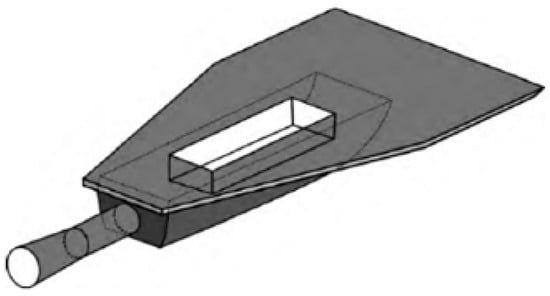
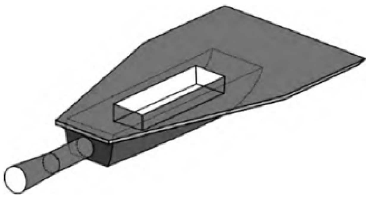
To establish a spectrum prediction model for high-speed vehicle cavities, wind tunnel tests were conducted on the C201 cavity benchmark model (shown in Figure 1), from which complete aerodynamic characteristics and a noise database were obtained at test Mach numbers of 0.6, 0.9, 1.5, and 2.0. The tests were performed in the 0.6 m transonic and supersonic wind tunnel at the China Aerodynamics Research and Development Center, a semi-return intermittent blowdown tunnel whose test section has a cross-section of 0.6 m × 0.6 m and a length of 1.775 m. The tunnel operates over a Mach number range of 0.4 to 3.0, which fully covers the typical flight conditions of high-speed vehicles from subsonic to supersonic speeds.

Figure 1. C201 cavity benchmark model.

2.1. Wind Tunnel Test of the C201 Cavity Benchmark Model

This study selected the C201 cavity benchmark model as the scaled test object for typical cavity structures of high-speed vehicles. The structure of the plate–cavity test model is shown in Figure 1. To promote full development of the turbulent boundary layer, a flat plate approximately 200 mm long was installed upstream of the cavity leading edge.

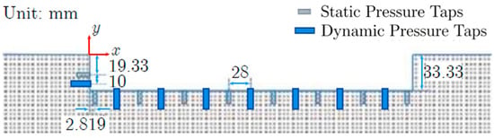
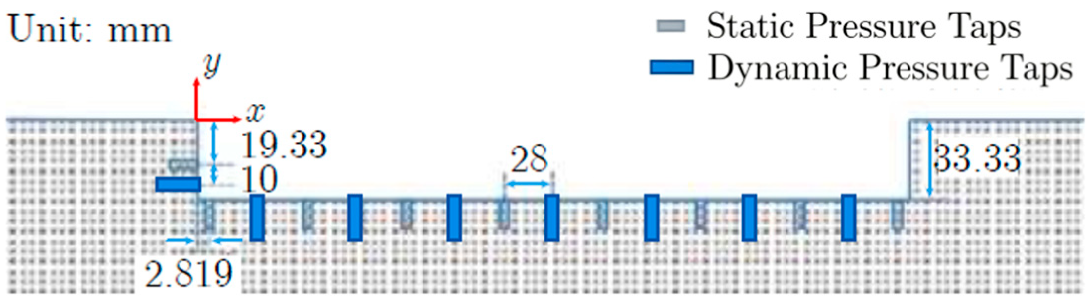
The model measures 514 mm in overall length and 320 mm in width, the cavity has a length of L = 200 mm, a depth of D = 33.33 mm, and a width of W = 66.67 mm. Static pressure taps and fluctuating pressure taps were arranged alternately on the sidewall near the leading edge and on the bottom surface of the cavity model, as illustrated in Figure 2. A total of 9 static pressure taps and 8 fluctuating pressure taps were installed, of which 1 static pressure tap and 1 fluctuating pressure tap were placed on the sidewall near the leading edge. The remaining taps were distributed evenly along the central axis of the bottom surface, with a spacing of 28 mm between adjacent static and fluctuating pressure taps. The fluctuating pressure sensors installed on the test model are piezoresistive transducers of type XCE-062, with a measurement range of 15 psi, a natural frequency of 200 kHz and a sampling frequency of 50 kHz. A PSI 9016 electronically scanned pressure (ESP) system is used to measure the static pressure within the cavity; it has a range of 15 psi, a system accuracy of ±0.05% of full scale (FS), and a sampling rate of 100 samples per channel per second. During the tests, strain-gauge pressure transducers are employed to measure the total pressure in the settling chamber of the wind tunnel and the static pressure in the test section; the voltage signals are sampled, amplified and subjected to analog-to-digital conversion, and are finally processed by a computer, which provides the test data in real time.

Figure 2. Static and fluctuating pressure taps along the symmetric line on the cavity bottom.

Under inflow Mach numbers of 0.6, 0.9, 1.5, and 2.0, static and fluctuating pressure data of the cavity model were collected at angles of attack of −6°, −4°, −2°, 0°, and 2°. To characterize the distribution of the acoustic load on the cavity walls, the fluctuating pressure at the measurement points in the cavity flow field is expressed as the sound pressure level L_sp. The sound pressure level can be calculated from the time-domain AC signal p(t) acquired by the fluctuating pressure taps:

$$p_{\mathit{rms}}=\underset{T\to \infty }{\lim }\sqrt{{\displaystyle \frac{1}{T}}{\displaystyle {\int }_0^T{p}^2(t)}\mathit{dt}}$$

(1)

$$L_{\mathit{sp}}=20\lg {\displaystyle \frac{p_{\mathit{rms}}}{p_{\mathit{ref}}}}$$

(2)

where p_rms is the root mean square (RMS) value of the fluctuating pressure, T is the sample length, and p_ref = 2 × 10⁻⁵ Pa is the reference pressure.

2.2. Ensemble Learning Prediction Models

To construct a high-precision prediction model for the cavity noise spectra of high-speed vehicles, this study adopts three ensemble learning models that perform well on complex regression tasks: Random Forest (RF), XGBoost (Extreme Gradient Boosting), and LightGBM (Light Gradient Boosting Machine). These models respectively represent the Bagging ensemble and two mainstream gradient boosting frameworks, and offer strong nonlinear fitting capability, with promising applications in modeling complex flows in aerospace engineering. To comprehensively assess the advantages of ensemble learning, the Support Vector Machine (SVM) is additionally introduced as a baseline for comparison, underscoring the particular value of ensemble learning for the strongly nonlinear, flow-induced noise of high-speed vehicle cavities.

2.2.1. Random Forest

Random Forest is an algorithm built on the Bagging ensemble learning strategy. It reduces model variance and improves the prediction accuracy by constructing multiple decision trees and aggregating their predictions. In regression tasks, given an input feature vector X ∈ ℝ^p (where p is the number of feature dimensions), the final prediction $\widehat{y}\left(X\right)$ of the Random Forest is the arithmetic mean of the predictions of all K decision trees T_k(X):

$$\widehat{y}\left(X\right)={\displaystyle \frac{1}{K}}{\displaystyle \sum _{k=1}^K{T}_k}\left(X\right)$$

(3)

During the growth of an individual decision tree, features and split points are selected iteratively to construct the tree structure. In regression problems, a commonly used splitting criterion is to minimize the Mean Squared Error (MSE) of the nodes:

$$\mathit{MSE}\left(D\right)={\displaystyle \frac{1}{N}}{{\displaystyle \sum _{i\in D}\left(y_i-{\overline{y}}_D\right)}}^2$$

(4)

where D is the set of samples in the current decision tree node, N is the number of samples in node D, y_i is the true target value of the i-th sample, and ${\overline{y}}_D$ is the mean of the target values of all samples in the node.

In this study, the random forest is configured with 100 trees, a minimum leaf size of 5, two predictors sampled at each split, and a bootstrap fraction of 1.0.

2.2.2. XGBoost

XGBoost is an efficient implementation of Gradient Boosting Decision Trees (GBDT). It controls model complexity through second-order derivative information and explicit regularization terms, thereby striking a balance between accuracy and efficiency. XGBoost adopts an additive model: at the t-th iteration, a new tree is added to the current model to minimize the following objective function:

$$L^{\left(t\right)}={\displaystyle \sum _{i=1}^{n}l\left(y_i,F_{t-1}\left(X_i\right)+f_t\left(X_i\right)\right)+\mathit{\Omega }}\left(f_t\right)$$

(5)

where L^(t) is the total objective function at the t-th iteration, l is a differentiable loss function, F_t−1(X_i) is the cumulative prediction of the model for sample i after the first t−1 iterations, f_t(X_i) is the prediction of the newly added tree for sample i at the t-th round, and Ω(f_t) is the regularization term for the t-th tree. The regularization term Ω(f) takes the specific form:

$$\mathit{\Omega }\left(f\right)=\mathit{\gamma T}+{\displaystyle \frac{1}{2}}\lambda {\displaystyle \sum _{j=1}^T{\omega }_j^2}$$

(6)

where γ is the minimum loss-reduction threshold for splitting a leaf node, T is the total number of leaf nodes in the decision tree, λ is the L2 regularization coefficient, and ω_j is the output value of the j-th leaf node.

To facilitate efficient optimization, XGBoost applies a second-order Taylor expansion to the loss function. Let $g_i={\partial }_{{\widehat{y}}_{t-1}}l\left(y_i,{\widehat{y}}_{t-1}\right)$ and $h_i={\partial }_{{\widehat{y}}_{t-1}}^{2}l\left(y_i,{\widehat{y}}_{t-1}\right)$ denote the first- and second-order gradients of the loss function with respect to the current prediction, respectively. After removing the constant terms, the approximate objective function at the t-th iteration under a fixed tree structure becomes:

$${\tilde{L}}^{\left(t\right)}={\displaystyle \sum _j^T\left[\left({\displaystyle \sum _{i\in I_j}{g}_i}\right){\omega }_j+\frac{1}{2}\left({\displaystyle \sum _{i\in I_j}{h}_i+\lambda }\right){\omega }_j^2\right]}+\mathit{\gamma T}$$

(7)

where I_j is the set of samples assigned to the j-th leaf node. For a fixed tree structure, the optimal leaf weight ${\omega }_j^{*}$ and the corresponding objective function value are respectively:

$${\omega }_j^{*}=-{\displaystyle \frac{{\displaystyle \sum _{i\in I_j}{g}_i}}{{\displaystyle \sum _{i\in I_j}{h}_i+\lambda }}}$$

(8)

$${\tilde{L}}^{\left(t\right)}\left(q\right)=-{\displaystyle \frac{1}{2}}{\displaystyle \sum _{j=1}^T\frac{{\left({\displaystyle \sum _{i\in I_j}{g}_i}\right)}^2}{{\displaystyle \sum _{i\in I_j}{h}_i+\lambda }}}+\mathit{\gamma T}$$

(9)

where q is the function that maps a sample to a leaf index, i.e., the structure of the tree.

When splitting a node, XGBoost uses a greedy algorithm to select the feature and split point that reduce ${\tilde{L}}^{\left(t\right)}$ the most. The split gain is computed as:

$$\mathit{Gain}={\displaystyle \frac{1}{2}}\left[{\displaystyle \frac{G_L^2}{H_L+\lambda }}+{\displaystyle \frac{G_R^2}{H_R+\lambda }}-{\displaystyle \frac{G_L+G_R}{H_L+H_R+\lambda }}\right]-\gamma$$

(10)

where $G_L={\displaystyle \sum _{i\in I_L}{g}_i}$, $H_L={\displaystyle \sum _{i\in I_L}{h}_i}$.

In this study, XGBoost is configured with 50 boosting iterations, a maximum tree depth of 5, a learning rate of 0.1, a minimum child weight of 1, a row (instance) subsampling ratio of 0.95, a column (feature) subsampling ratio of 1.0, an L1 regularization coefficient of 0, and an L2 regularization coefficient of 1.

2.2.3. LightGBM

LightGBM is another efficient gradient boosting framework, designed to accelerate training on large-scale data while reducing memory consumption. Its core techniques include Gradient-based One-Side Sampling (GOSS) and Exclusive Feature Bundling (EFB). Although LightGBM computes the split gain in a form consistent with that of XGBoost, it incorporates substantial optimizations in the implementation details:

$$\mathit{Gain}={\displaystyle \frac{1}{2}}\left[{\displaystyle \frac{{\left({\displaystyle \sum _{i\in I_L}{g}_i}\right)}^2}{{\displaystyle \sum _{i\in I_L}{h}_i+\lambda }}}+{\displaystyle \frac{{\left({\displaystyle \sum _{i\in I_R}{g}_i}\right)}^2}{{\displaystyle \sum _{i\in I_R}{h}_i+\lambda }}}-{\displaystyle \frac{{\left({\displaystyle \sum _{i\in I}{g}_i}\right)}^2}{{\displaystyle \sum _{i\in I}{h}_i+\lambda }}}\right]-\gamma$$

(11)

where I_L and I_R are the sample sets of the left and right leaf nodes after the split, respectively.

The core idea is that, when computing the gain, it retains samples with large absolute gradient values and randomly samples those with small gradients rather than using all samples. This substantially reduces the computational burden without appreciably increasing bias, making LightGBM particularly well suited to the large-scale, high-dimensional, complex datasets encountered in predicting the cavity noise spectra of high-speed vehicles.

In this study, LightGBM is configured with a maximum of 60 boosting iterations, an early-stopping patience of 30 rounds, 10 leaves per tree, a maximum tree depth of 7, a learning rate of 0.1, a minimum of 20 data points per leaf, a bagging fraction and a feature fraction of 0.7 each, and no regularization.

2.2.4. Support Vector Machine

Support Vector Machine Regression (SVR) is a kernel method based on the structural risk minimization principle of statistical learning theory. Its goal is to find a regression function such that most samples fall within an ε-insensitive tube of width 2ε centered on this function. The standard formulation of the SVM is expressed as a convex optimization problem:

$$\underset{W,b,\xi {\xi }^{*}}{\min }{\displaystyle \frac{1}{2}}{‖W‖}^2+C{\displaystyle \sum _{i=1}^m\left({\xi }_i+{\xi }_i^{*}\right)}$$

(12)

The constraints are:

$$\left\{\begin{array}{l}{y}_i-\left(W^T\phi \left(X_i\right)+b\right)\le \epsilon +{\xi }_i\\ \left(W^T\phi \left(X_i\right)+b\right)-y_i\le \epsilon +{\xi }_i^{*}\\ {\xi }_i,{\xi }_i^{*}\ge 0,i=,\dots ,m\end{array}\right.$$

(13)

where W is the weight vector in the high-dimensional feature space, b is the bias term, φ(⋅) is a nonlinear mapping function, C is the regularization parameter that balances model complexity, ε is the insensitive loss parameter that defines the radius of the tube, ξ_i and ${\xi }_i^{*}$ are the slack variables for the upper and lower boundaries associated with the i-th sample, which handle samples falling outside the tube, and m is the total number of training samples.

By solving the above optimization problem using the Lagrangian multiplier method, the final SVM regression function is obtained as:

$$f\left(X\right)={\displaystyle \sum _{i=1}^m\left({\alpha }_i-{\alpha }_i^{*}\right)K\left(X_i,X\right)+b}$$

(14)

where α_i and ${\alpha }_i^{*}$ are Lagrange multipliers, and $K\left(X_i,X\right)=\mathrm{\phi }{\left(X_i\right)}^T\mathrm{\phi }\left(X\right)$ is the kernel function. For the support vector machine, a radial basis function (RBF) kernel is adopted; being a local kernel, its value decays rapidly as the distance between samples increases, with the result that when the sample to be predicted lies far from all support vectors, the regression function degenerates to the bias constant b. The baseline configuration is specified by a box constraint C = 1, ε = 0.1 and a kernel scale (KernelScale) σ = 1, corresponding to γ = 1/σ² = 1.

2.3. Bayesian Optimization

During model training, the accuracy ability of a model depend strongly on its hyperparameter values; efficiently locating optimal hyperparameters is therefore a core task in machine learning modeling. The most commonly used search methods are random search and grid search, which are easy to implement and cover a wide search space. Their drawback, however, is that each new hyperparameter combination is tested without making full use of the information from previously sampled points. When the hyperparameter space is high-dimensional, such methods often consume substantial computational resources and require long processing times.

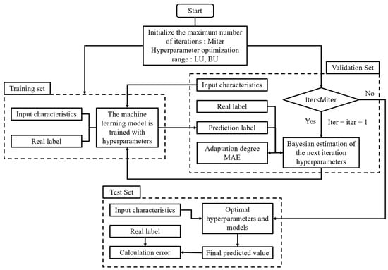
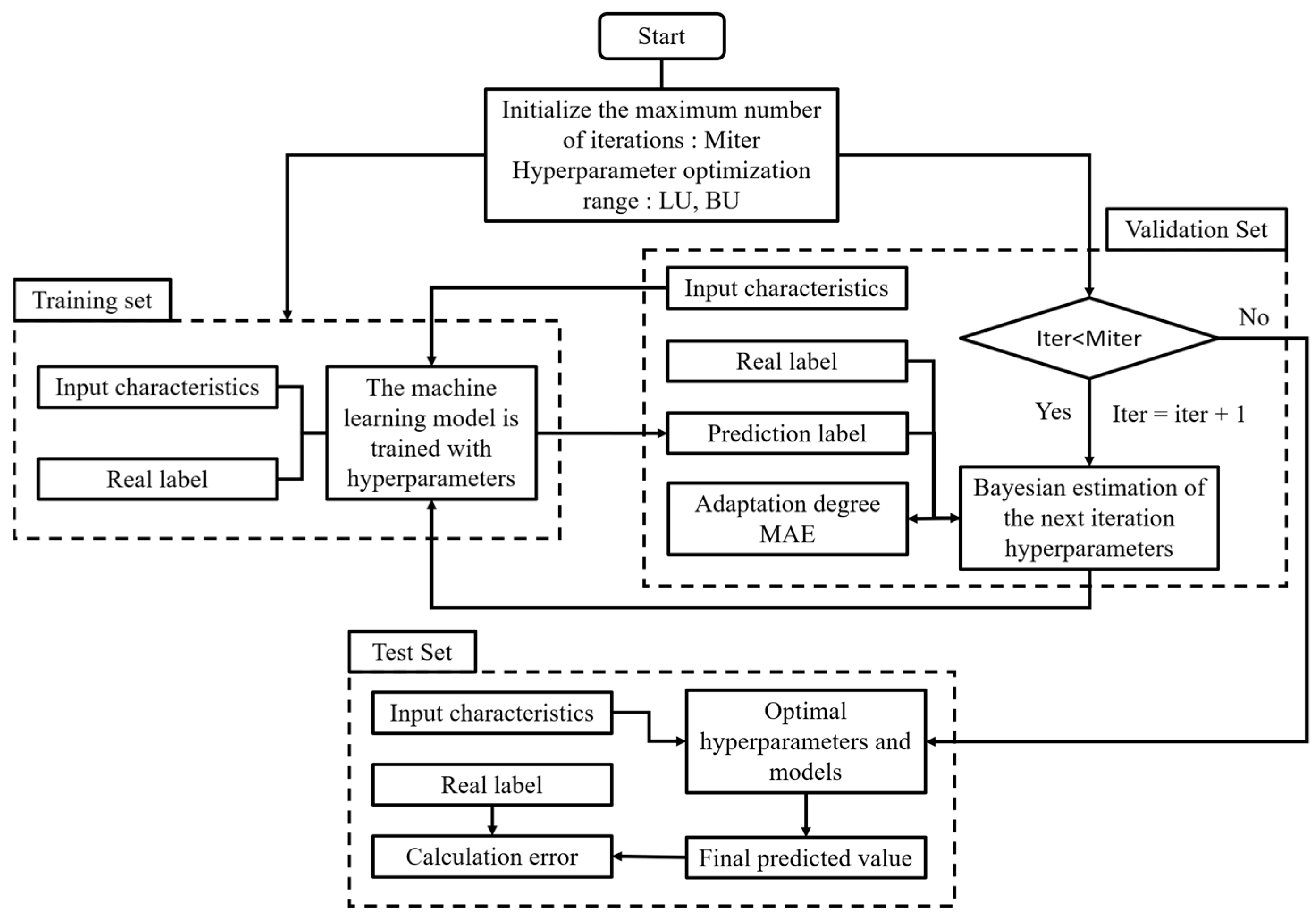
In contrast, Bayesian optimization uses Bayes’ theorem to model the posterior distribution of the objective function from the existing data, and then selects the next most promising hyperparameter combination accordingly. This method fully leverages historical sampling information: by learning the shape of the objective function, it progressively guides the search toward the global optimum. The implementation proceeds as follows (Figure 3):

Figure 3. Principles and process of Bayesian optimization.

• Define the hyperparameter space: determine the hyperparameters to be optimized and their respective value ranges.
• Define a surrogate model: select an appropriate surrogate model to approximate the objective function.
• Initialize the sample set: randomly select several initial samples in the hyperparameter space and train the surrogate model on the performance evaluations of these samples.
• Iterative optimization: according to the predictions of the surrogate model, select the hyperparameter combination most likely to improve model performance; evaluate this combination on the actual model and record its performance; incorporate the new sample into the training set and update the surrogate model’s estimate of the objective function; and repeat these steps until the preset number of iterations is reached or the specified stopping criteria are met.
• Output the best hyperparameters: based on the optimization results, output the best-performing hyperparameter combination for training the final model.

Bayesian optimization is implemented using a Gaussian process surrogate model together with the expected-improvement-plus acquisition function, with the root-mean-square error on the validation set adopted as the optimization criterion. Whereas the optimization settings are common to all models, the search ranges and optimal values of the hyperparameters differ between the two prediction tasks and are therefore reported in the corresponding sections below.

3. Analysis of Prediction Results of Ensemble Learning Models for Cavity Noise Spectra

To systematically evaluate the applicability and the predictive capability under unseen conditions of ensemble learning models in predicting the cavity noise spectra of high-speed vehicles. Based on the typical flight conditions of high-speed vehicles, the test data are divided into a model training set and an unseen-condition test set. The former encompasses multiple high-speed incoming-flow conditions with Mach numbers of 0.6, 0.9, 1.5 and 2.0, angles of attack ranging from −6° to 2°, and multiple measurement locations inside the cavity, and is used for learning the model parameters; the latter consists exclusively of conditions that are not used in training, so as to examine the predictive capability of the models under unseen conditions and thereby bring the evaluation closer to the variable operating conditions and complex layouts encountered in the practical engineering of high-speed vehicles. The data used for model training were randomly divided into training, validation, and test subsets in an 8:1:1 ratio, with Mach number, angle of attack, measurement point position, and frequency serving as input features and the sound pressure amplitude at different frequencies as the output feature. In all cases, the random seed is fixed at 1 and both the input and the output features are standardized by Z-score normalization, with the standardization statistics estimated solely from the training set and subsequently applied to the validation set, the test set and the data of the prediction tasks, thereby preventing data leakage. A Fourier transform was performed on the measured fluctuating pressure data. For each test condition, a database comprising 1147 amplitude–frequency points over the frequency range of 6–7000 Hz is constructed separately for each of the eight fluctuating-pressure measurement points inside the cavity, and the three ensemble learning models together with the SVM are trained on the basis of this database.

For model evaluation, the coefficient of determination R², root mean square error (RMSE), and mean absolute error (MAE) were adopted as metrics, computed as follows:

$$R^2=1-{\displaystyle \frac{\mathit{SSE}}{\mathit{SST}}}=1-{\displaystyle \frac{{\displaystyle \sum _{i=1}^n{\left(y_i-{\widehat{y}}_i\right)}^2}}{{\displaystyle \sum _{i=1}^n{\left(y_i-{\overline{y}}_i\right)}^2}}}$$

(15)

$$\mathit{RMSE}=\sqrt{\mathit{MSE}}=\sqrt{{\displaystyle \frac{1}{n}}{\displaystyle \sum _{i=1}^n{\left(y_i-{\widehat{y}}_i\right)}^2}}$$

(16)

$$\mathit{MAE}={\displaystyle \frac{1}{n}}{\displaystyle \sum _{i=1}^n\left|y_i-{\widehat{y}}_i\right|}$$

(17)

Here, the gap is defined as 100 × (RMSE_val − RMSE_train)/RMSE_train and is expressed as a percentage, which is used to quantify the degree of overfitting.

For the unseen-condition prediction task, the dominant-frequency amplitude error is adopted as the evaluation metric in this study. The engineering significance of this criterion lies in the fact that, in the practice of cavity noise control, the dominant-frequency amplitude directly determines the peak noise level and therefore constitutes an indicator that is more closely aligned with engineering requirements than the average error over the entire frequency band.

3.1. Results and Analysis of the Spatial-Position Prediction Task

Table 1 presents the data partitioning of the model training set and the unseen-condition test set for the spatial-position prediction task, in which measurement point P1 (x/L = 0) is located at the leading edge of the cavity, P6 (x/L = 0.644) near the trailing edge, and P8 (x/L = 0.924) at the trailing edge.

Table 1. Data partitioning of the model training set and the unseen-condition test set for the spatial-position prediction task.

Dataset	Mach Number	Angle of Attack α/(°)	Measurement Point Position
Training Set	0.6	−6, −4, −2, 0, 2	P1~P8
	0.9	−6, −4, −2, 0, 2	P1~P8
	1.5	−6, −2, 0, 2	P2, P3, P4, P5, P7
	2.0	−6, −4, −2, 0, 2	P1~P7
Unseen-Condition Test Set	1.5	−4	P1, P6, P8

Table 2 presents the evaluation metrics obtained by each model during training for the spatial-position prediction task. Before hyperparameter tuning, RF achieves the highest prediction accuracy in this task, consistently outperforming the others on all three metrics across the three datasets, followed by LightGBM; the training–validation gaps of the two models are 2.24% and 1.90%, respectively, which are of the same order of magnitude, with neither exhibiting evident overfitting. Although the prediction error of XGBoost is markedly higher than those of the two aforementioned models, its training–validation gap of 0.89% does not exceed those of RF and LightGBM, indicating that its elevated error stems from insufficient fitting capacity rather than from degradation of predictive performance. The accuracy of the SVM is significantly lower than that of the remaining models; on the whole, RF emerges—when prediction accuracy is taken as the criterion—as the most accurate model for this task, followed by LightGBM, with the difference between them being relatively small.

Table 2. Evaluation metrics of different machine learning models for the spatial-position prediction task.

Model	Training Set			Validation Set			Test Set
	R2	RMSE	MAE	R2	RMSE	MAE	R2	RMSE	MAE
RF	0.94724	2.0805	1.4601	0.94493	2.1271	1.4876	0.94564	2.1059	1.4754
XGBoost	0.92561	2.4705	1.6536	0.92438	2.4926	1.6683	0.92617	2.4543	1.6475
LightGBM	0.94437	2.1365	1.4973	0.94231	2.1772	1.5139	0.94335	2.1498	1.5008
SVM	0.68737	5.0645	3.9896	0.68483	5.0887	4.0097	0.69160	5.016	3.9315

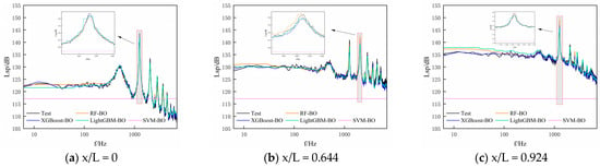
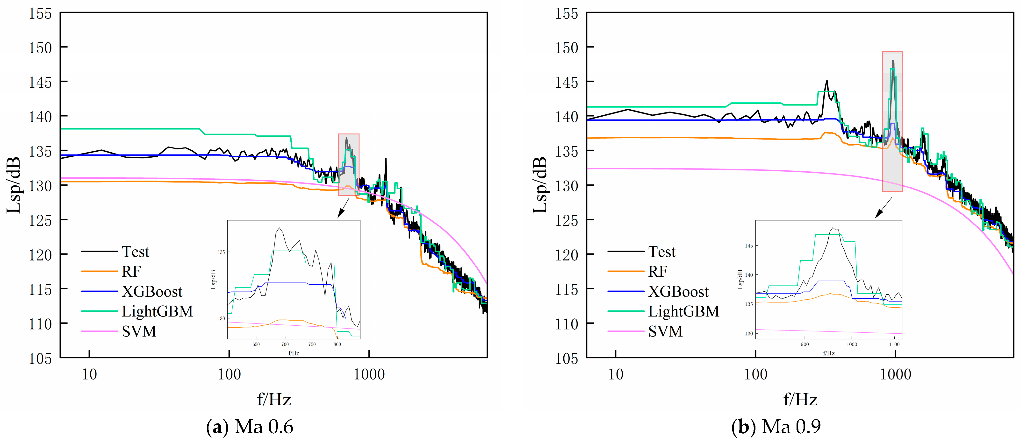
Figure 4 presents the prediction results of the three ensemble learning models and the SVM for the cavity wall sound pressure spectra under three groups of unseen conditions, namely a Mach number of 1.5, an angle of attack of −4° and measurement points P1, P6 and P8, while Table 3 compares the dominant-frequency amplitudes predicted by each model with the measured values at the three measurement points. In terms of the mean absolute error, RF achieves the highest accuracy (13.36 dB), followed by LightGBM (13.95 dB) and XGBoost (14.96 dB), whereas the SVM yields 20.51 dB. The difference between RF and LightGBM is only 0.58 dB, indicating that the two models perform at a comparable level. A point-by-point comparison shows that LightGBM slightly outperforms RF at P6 and P8, whereas RF exhibits a more pronounced advantage at P1, and it is this difference that governs the ranking of the average values. The SVM is the least accurate of the four models at all three measurement points, with its predicted curves degenerating to an almost horizontal line that fails to reproduce the peaks and valleys of the spectra.

Figure 4. Spatial-position prediction results.

Table 3. Comparison of predicted and measured dominant-frequency amplitudes in spatial-position prediction task (Unit dB).

Model	P1		P6		P8
	Amplitude	Difference	Amplitude	Difference	Amplitude	Difference
Test	143.73	-	141.95	-	148.82	-
RF	127.58	16.15	129.55	12.4	137.28	11.54
XGBoost	124.1	19.63	128.95	13	136.56	12.26
LightGBM	124.07	19.66	129.74	12.21	138.85	9.97
SVM	116.31	27.42	124.67	17.28	132	16.82

All the results presented above are obtained under the default or fixed hyperparameter configurations of each model. Given that hyperparameters exert a considerable influence on the performance of ensemble models, this section further employs Bayesian optimization to tune the hyperparameters of each model. Table 4 presents the search ranges and optimal values of the hyperparameters of each model for the spatial-position prediction task, with the baseline values also listed for comparison.

Table 4. Search ranges and optimal values of the hyperparameters for the spatial-position prediction task.

Model	BO Iterations	Hyperparameter	Baseline	Search Range	Optimal Value
RF	20	Minimum leaf size	5	[1, 15]	1
		Predictors per split	2	[1, 5]	5
XGBoost	30	Boosting iterations	50	[100, 1000]	978
		Maximum depth	5	[3, 12]	12
		Learning rate	0.1	[0.01, 0.3]	0.2295
		Minimum child weight	1	[5, 30]	5
		Subsample ratio	0.95	[0.5, 1.0]	0.9910
		Column subsample ratio	1	[0.5, 1.0]	0.8711
LightGBM	30	Boosting iterations	60	-	1612
		Early stopping patience	30	-	50
		Number of leaves	10	[10, 300]	207
		Maximum depth	7	[3, 15]	15
		Learning rate	0.1	[0.01, 0.3]	0.0911
SVM	25	Box constraint C	1	[1, 10,000]	2.928
		Kernel scale σ	1	[0.1, 5]	0.1575

It should be noted that XGBoost and LightGBM differ in the manner in which the number of boosting iterations is determined. For XGBoost, this number is treated as a hyperparameter and is included in the search, whereas LightGBM adopts an early-stopping mechanism in which the number of iterations is excluded from the search and the training is instead terminated adaptively according to the early-stopping criterion. Despite this difference in mechanism, both models make use of validation-set information in determining the number of iterations; the symmetry of information usage therefore holds and the comparison between them remains fair.

In addition, owing to the training complexity of O(n²)–O(n³), a staged subsampling strategy is adopted for the SVM in this study. The hyperparameter search is performed on a subset of 8000 rows, which is randomly drawn once more from the training subset so as to ensure consistency in the distribution of test conditions; once the optimal hyperparameters have been determined, the final model is retrained on a stratified subset of 39,878 rows. In the stratified sampling, the samples are grouped according to the unique combinations of the test condition parameters, and an equal number of frequency points is randomly drawn from each group, thereby preserving in the subset the distribution of each condition as it appears in the full training set. The random seed is fixed at 1 for the sampling.

Table 5 presents the evaluation metrics of each model after Bayesian optimization for the spatial-position prediction task. Since the validation set participates in model selection, its metrics are subject to selection bias and are, therefore, optimistic; accordingly, the comparison in the following is based on the test set.

Table 5. Evaluation metrics of each model after Bayesian optimization for the spatial-position prediction task.

Model	Training Set			Validation Set			Test Set
	R2	RMSE	MAE	R2	RMSE	MAE	R2	RMSE	MAE
RF	0.9967	0.5211	0.4145	0.9946	0.6614	0.5115	0.9947	0.6598	0.513
XGBoost	0.9991	0.2654	0.2067	0.9956	0.5975	0.4703	0.9957	0.5927	0.4657
LightGBM	0.9932	0.7473	0.5619	0.9918	0.8183	0.6136	0.9921	0.8024	0.6046
SVM	0.9795	1.299	0.7819	0.9748	1.431	0.8719	0.9761	1.3992	0.8587

Compared with Table 2, hyperparameter optimization substantially improves the in-distribution accuracy of all four models; notably, however, it also alters their relative ranking, with RF achieving the highest accuracy at the baseline stage, followed by LightGBM and then XGBoost, whereas after optimization XGBoost rises to first place—followed by RF and, then, LightGBM—the improvement of XGBoost being the largest among the four models. At the same time, the optimization generally increases the degree of overfitting, most prominently for XGBoost, whose optimal solution lies at the boundary of the search space; nevertheless, XGBoost still attains the highest test-set accuracy, indicating that in this task the gains derived from its enhanced fitting capacity outweigh the cost of the increased variance.

It should be pointed out that the staged subsampling strategy renders the optimization effect reported here for the SVM conservative: after Bayesian optimization, the number of training samples used by the model is reduced by approximately 72% relative to the baseline, whereas the RMSE on the test set nevertheless decreases from 5.0160 to 1.3992. Had the optimized model been trained on the full sample set, its accuracy would be no lower than the values reported here, and the subsampling therefore does not exaggerate the benefit of hyperparameter tuning for the SVM.

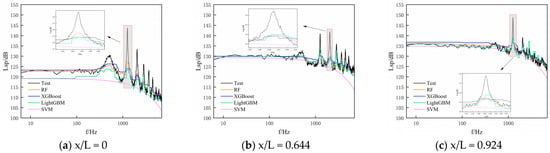
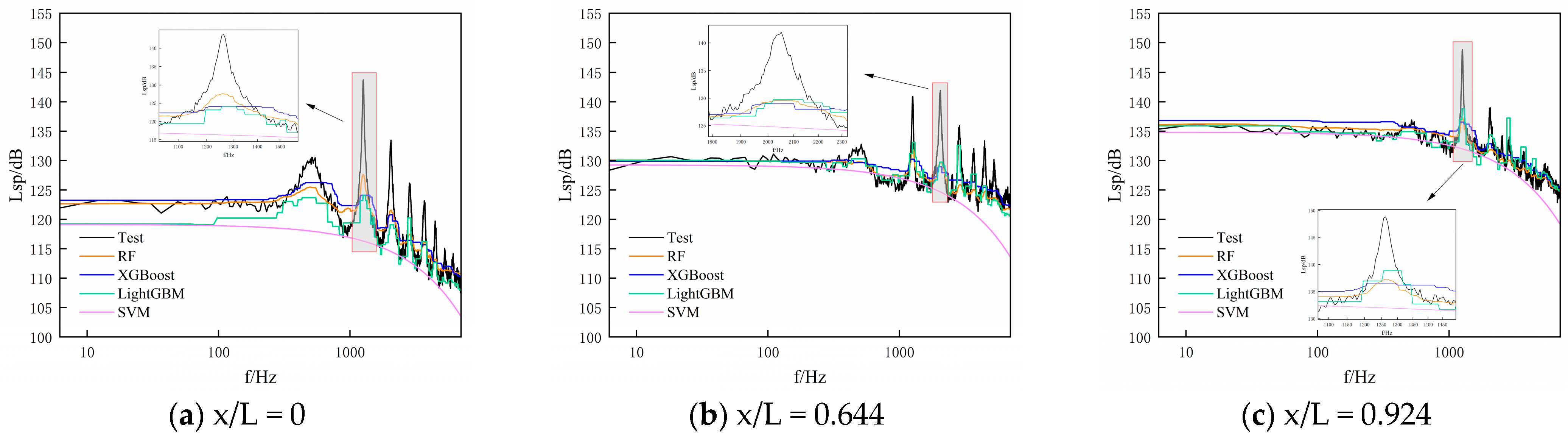
Table 6 presents the comparison between the predicted and measured dominant-frequency amplitudes of each model after Bayesian optimization under the unseen conditions (measurement points P1, P6 and P8), and Figure 5 shows the corresponding complete spectra. The errors of all three ensemble models decrease substantially. In terms of the accuracy of the dominant-frequency amplitude, XGBoost and RF are essentially comparable after tuning, differing by only 0.09 dB, whereas LightGBM ranks third. This ranking is not consistent with that at the baseline stage, indicating that the benefit of hyperparameter optimization differs markedly among the models: XGBoost, whose baseline error is the largest, gains the most from tuning, whereas LightGBM, which performs relatively well at the baseline, gains the least. The predicted peak amplitudes of all four models are lower than the measured values, exhibiting a systematic underestimation that is consistent with the tendency of regression models trained under a mean-square-error criterion to shrink toward the center of the distribution; although the magnitude of the underestimation is reduced after tuning, it is not entirely eliminated.

Table 6. Comparison of predicted and measured dominant-frequency amplitudes after Bayesian optimization for the spatial-position prediction task (Unit dB).

Model	P1		P6		P8
	Amplitude	Difference	Amplitude	Difference	Amplitude	Difference
Test	143.73	-	141.95	-	148.82	-
RF	139.98	3.75	139.69	2.26	147.97	0.85
XGBoost	141.78	1.95	139.52	2.43	146.61	2.21
LightGBM	141.68	2.05	139.03	2.92	145.66	3.16
SVM	117.11	26.62	117.11	24.84	117.11	31.71

Figure 5. Spatial-position prediction results after Bayesian optimization.

The situation for the SVM stands in stark contrast to that of the three ensemble models: after tuning, its dominant-frequency amplitude error tends to increase, and the predicted values at the three measurement points are identical, all being 117.11 dB, which differs from the mean of the training targets (117.0881 dB) by only 0.022 dB, indicating that the output has degenerated to a constant. This shows that the radial basis function kernel ceases to be effective under unseen conditions: as the distance between the condition to be predicted and the training conditions increases, the kernel values decay rapidly, so that the sum of the kernel terms in the decision function tends to zero and the output degenerates to the bias constant, which corresponds to the mean of the training targets after inverse normalization. Since Bayesian optimization is guided by the validation-set error, it tends to select a narrower kernel so as to enhance in-distribution fitting, thereby further aggravating this degeneration.

3.2. Results and Analysis of the Flow-Condition Prediction Task

Table 7 presents the data partitioning of the model training set and the unseen-condition test set for the flow-condition prediction task.

Table 7. Data partitioning of the model training set and the unseen-condition test set for the flow-condition prediction task.

Dataset	Mach Number	Angle of Attack α/(°)	Measurement Point Position
Training Set	0.6	−6, −4, −2, 2	P1~P8
		0	P1~P7
	0.9	−6, −4, −2, 2	P1~P8
		0	P1~P7
	1.5	−6, −4, −2, 2	P1~P8
		0	P1~P7
	2.0	−6, −4, −2, 2	P1~P8
		0	P1~P7
Unseen-Condition Test Set	0.6	0	P8
	0.9	0	P8
	1.5	0	P8
	2.0	0	P8

Table 8 records the evaluation metrics of the four models during training for the flow-condition prediction task. In terms of prediction accuracy, RF ranks highest in this task: it attains the highest coefficient of determination and the lowest RMSE and MAE on the training, validation and test sets alike, that is, it consistently outperforms the remaining models on all three metrics across the three datasets, followed by LightGBM, whose difference from RF is relatively small. With regard to training–validation consistency, the gap of LightGBM is 0.83%, smaller than the 2.49% of RF, indicating that LightGBM is slightly more stable whereas RF exhibits signs of mild overfitting; nevertheless, RF still achieves the higher absolute accuracy of the two. The prediction error of XGBoost is markedly higher than those of the two aforementioned models, while its training–validation gap of 0.89% does not exceed those of RF and LightGBM, pointing to insufficient fitting capacity. The accuracy of the SVM is significantly lower than that of the remaining models, and its training–validation gap of only 0.32% similarly points to insufficient fitting capacity. Taken together, with prediction accuracy taken as the criterion, RF is the most accurate model for this task, whereas LightGBM attains a comparable accuracy together with slightly better stability, so that both models are of engineering value under the accuracy requirements of this task; in contrast, the accuracy of XGBoost and the SVM in this task is insufficient to meet the requirements of practical application.

Table 8. Evaluation metrics of different machine learning models for the flow-condition prediction task.

Model	Training Set			Validation Set			Test Set
	R2	RMSE	MAE	R2	RMSE	MAE	R2	RMSE	MAE
RF	0.95046	2.008	1.4058	0.94781	2.0579	1.4337	0.94836	2.0369	1.4296
XGBoost	0.9241	2.4855	1.675	0.9225	2.5076	1.6888	0.92422	2.4675	1.6729
LightGBM	0.94496	2.1166	1.5236	0.94386	2.1342	1.5308	0.94364	2.1279	1.5284
SVM	0.68094	5.0959	4.0016	0.67789	5.1123	4.0107	0.68219	5.0531	3.9551

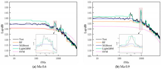
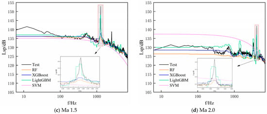
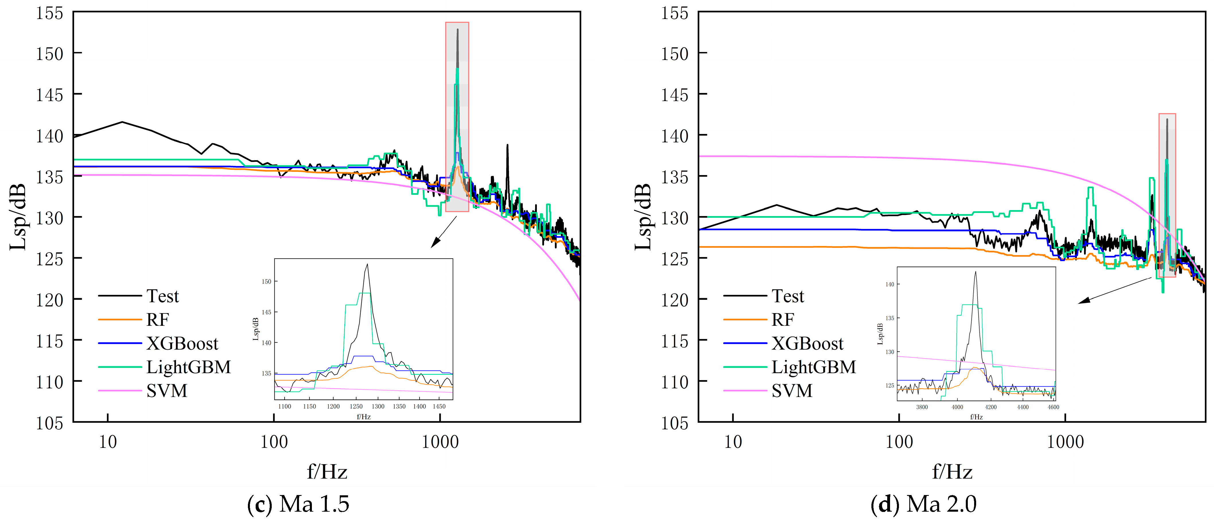
Figure 6 presents the prediction results of the three ensemble learning models and the SVM for the cavity wall sound pressure spectra at measurement point P8 (x/L = 0.924) with an angle of attack of 0° under four groups of unseen conditions corresponding to Mach numbers of 0.6, 0.9, 1.5 and 2.0, while Table 9 compares the predicted and measured dominant-frequency amplitudes for the corresponding conditions. The mean absolute error of the dominant-frequency amplitude for LightGBM is 3.18 dB, which is lower than those of the remaining models under all four conditions. In terms of this criterion, LightGBM achieves the highest prediction accuracy of the dominant-frequency amplitude among the models compared in this study, with its advantage remaining consistent across all four conditions.

Figure 6. Flow-condition prediction results.

Table 9. Comparison of predicted and measured dominant-frequency amplitudes for the flow-condition prediction task (Unit dB).

Model	Ma0.6		Ma0.9		Ma1.5		Ma2.0
	Amplitude	Difference	Amplitude	Difference	Amplitude	Difference	Amplitude	Difference
Test	136.82	-	148.05	-	152.86	-	141.91	-
RF	129.88	6.94	136.67	11.38	136.07	16.79	127.66	14.25
XGBoost	132.67	4.15	138.93	9.12	137.79	15.07	127.4	14.51
LightGBM	135.08	1.74	146.84	1.21	148.05	4.81	136.96	4.95
SVM	129.52	7.3	130.29	17.76	132.31	20.55	128.33	13.58

This result is not consistent with the ranking of in-distribution fitting accuracy in Table 8, in which RF ranks highest. This discrepancy has a clear interpretation: the overall in-distribution fitting accuracy and the capability of capturing peak values under unseen conditions characterize different aspects of a model, the former measuring the fidelity of the waveform over the entire frequency band and the latter measuring the ability to predict the key features of the spectrum. The predicted peak values of all four models are likewise lower than the measured values, exhibiting a systematic underestimation. Furthermore, among the four conditions the prediction error is generally the largest at Ma = 1.5, which is also the condition with the highest measured dominant-frequency amplitude, indicating that a higher peak level entails greater prediction difficulty. The error of the SVM increases as the Mach number deviates further from the training distribution, which is consistent with the property of the RBF kernel that its value decays with distance outside the training distribution.

Table 10 presents the hyperparameter search ranges and optimal values obtained by Bayesian optimization for each model in the flow-condition prediction task.

Table 10. Search ranges and optimal values of the hyperparameters for the flow-condition prediction task.

Model	Hyperparameter	Baseline	Search Range	Optimal Value
RF	Minimum leaf size	5	[1, 15]	1
	Predictors per split	2	[1, 5]	5
XGBoost	Boosting rounds	50	[100, 1000]	988
	Maximum depth	5	[3, 12]	10
	Learning rate	0.1	[0.01, 0.3]	0.266
	Minimum child weight	1	[5, 30]	14
	Subsample ratio	0.95	[0.5, 1.0]	0.5968
	Column subsample ratio	1	[0.5, 1.0]	0.9962
LightGBM	Boosting iterations	60	-	1612
	Early stopping patience	30	-	50
	Number of leaves	10	[10, 300]	300
	Maximum depth	7	[3, 15]	15
	Learning rate	0.1	[0.01, 0.3]	0.1167

It should be noted that, in the flow-condition prediction task, Bayesian optimization is applied only to the three ensemble models, with the SVM excluded from tuning and its post-optimization prediction results not discussed. This treatment is based on the clear evidence already obtained in the spatial-position prediction task: after Bayesian optimization, although the RMSE of the SVM on the in-distribution test set improves, its dominant-frequency amplitude error under unseen conditions deteriorates instead, and the decision function has degenerated to a bias constant. This indicates that the failure of the SVM under unseen conditions does not stem from an improper hyperparameter configuration but from the locality of the RBF kernel. Since this failure is a limitation at the level of model structure, Bayesian optimization cannot bring about any substantial improvement. Given that the above evidence is already sufficient and that a single run of Bayesian optimization for the SVM is markedly time-consuming, further tuning of the SVM in the flow-condition task would be of little methodological value. Therefore, in the flow-condition prediction task the SVM is retained with its baseline results only, serving as a benchmark to delineate the boundary of the model’s applicability in this type of task.

Table 11 presents the evaluation metrics of each model after Bayesian optimization for the flow-condition prediction task. Compared with the baseline results (Table 8), the in-distribution accuracy of all three ensemble models improves significantly. It is worth emphasizing in particular that hyperparameter optimization alters the relative ranking of the models: at the baseline stage RF achieves the highest accuracy, followed by LightGBM, whereas after optimization XGBoost ranks first, followed by RF. The same reversal also occurs in the spatial-position prediction task, indicating that this reversal is robust across the prediction tasks considered in this study rather than an accidental outcome of a single task.

Table 11. Evaluation metrics of each model after Bayesian optimization for the flow-condition prediction task (Unit dB).

Model	Training Set			Validation Set			Test Set
	R2	RMSE	MAE	R2	RMSE	MAE	R2	RMSE	MAE
RF	0.9966	0.5235	0.4165	0.9945	0.6675	0.5153	0.9944	0.6711	0.5161
XGBoost	0.9977	0.4314	0.3408	0.9955	0.6045	0.4774	0.9954	0.6052	0.478
LightGBM	0.9932	0.7462	0.562	0.9916	0.8269	0.6136	0.9918	0.8134	0.6102

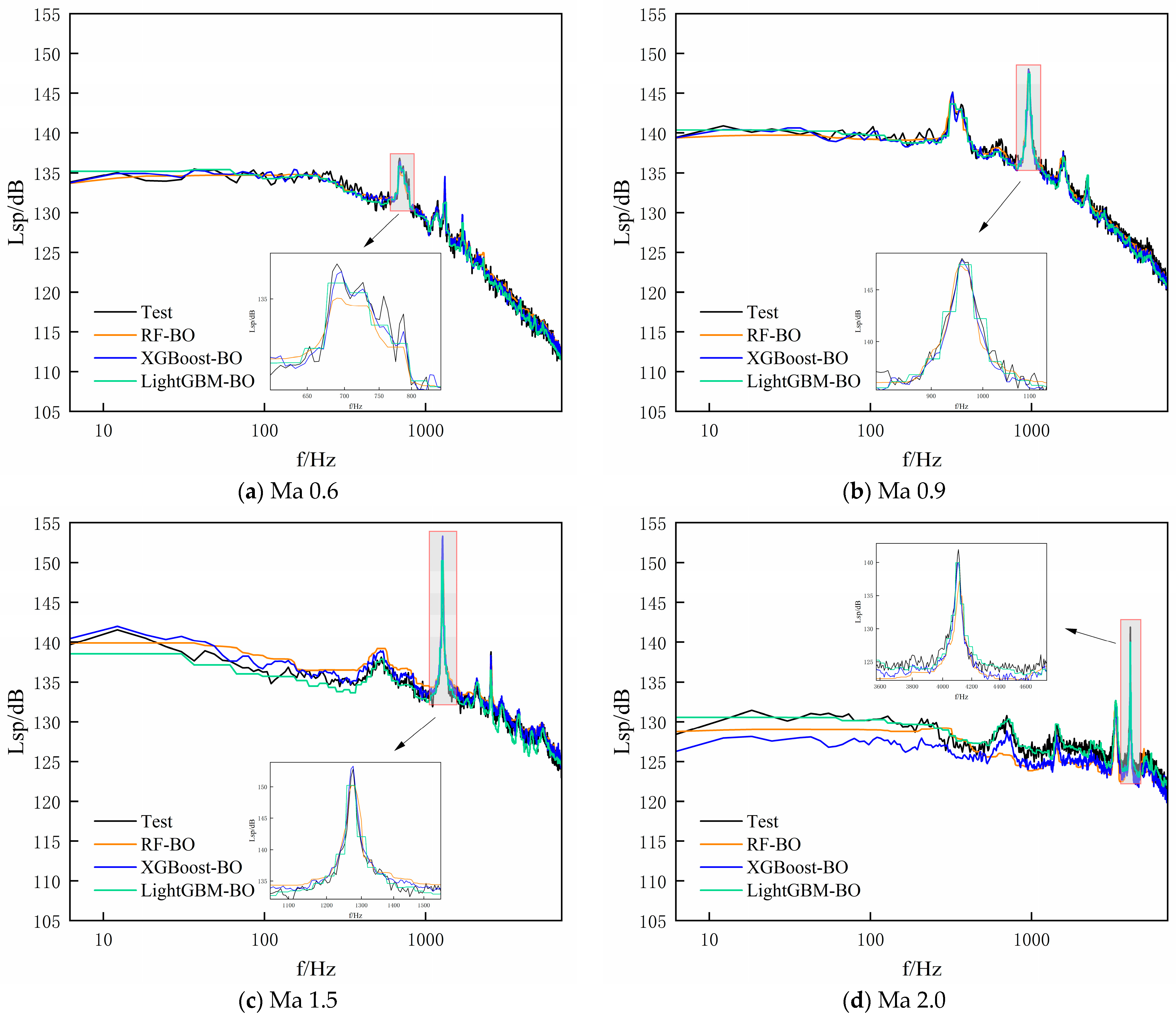
Table 12 presents the dominant-frequency amplitude prediction errors of each model after Bayesian optimization under four unseen Mach-number conditions for the flow-condition prediction task, and Figure 7 shows the corresponding complete spectra. The mean absolute error of XGBoost is 0.7575 dB, which is lower than those of the remaining models under all four conditions, that is, XGBoost consistently outperforms the others; LightGBM ranks second.

Table 12. Comparison of predicted and measured amplitudes after Bayesian optimization for the flow-condition prediction task.

Model	Ma0.6		Ma0.9		Ma1.5		Ma2.0
	Amplitude	Difference	Amplitude	Difference	Amplitude	Difference	Amplitude	Difference
Test	136.82	-	148.05	-	152.86	-	141.91	-
RF	135.04	1.78	147.26	0.79	150.26	2.6	136.18	5.73
XGBoost	136.28	0.54	147.91	0.14	153.3	−0.44	140	1.91
LightGBM	135.82	1	147.42	0.63	150.23	2.63	139.97	1.94

Figure 7. Flow-condition prediction results after Bayesian optimization.

4. Conclusions

This study addresses the prediction of cavity wall sound pressure spectra for high-speed vehicles. Within two types of prediction tasks—namely the flow-condition prediction task and the spatial-position prediction task—the performance of four models—RF, XGBoost, LightGBM and the SVM—is systematically compared, and the influence of Bayesian optimization on both the in-distribution fitting accuracy and the predictive capability under unseen conditions is examined. The main conclusions are as follows. (1) Hyperparameter optimization substantially improves the in-distribution accuracy and markedly reduces the dominant-frequency amplitude error under unseen conditions, although the magnitude of the improvement varies considerably from model to model. (2) Hyperparameter optimization alters the relative ranking of the models, and this reversal occurs consistently in both tasks: at the baseline stage RF and LightGBM are dominant, whereas after optimization XGBoost rises to first place. (3) Under unseen conditions the output of the SVM degenerates to the mean of the training targets; this failure stems from the locality of the radial basis function kernel and therefore constitutes a limitation at the level of model structure, which cannot be remedied by hyperparameter optimization.

These results indicate that no single model is optimal for all scenarios, and that model selection should be determined by jointly considering the prediction task, the evaluation objective and whether hyperparameter optimization is to be performed: in terms of the accuracy of reproducing the overall spectrum in distribution, XGBoost and RF are essentially comparable after optimization; in terms of the dominant-frequency amplitude accuracy under unseen conditions, XGBoost is clearly superior in the flow-condition prediction task, whereas in the spatial-position prediction task it is essentially on a par with RF. RF is the more robust choice when computational resources are limited and hyperparameter tuning cannot be implemented, since it is the best-performing model at the baseline stage both in distribution and under unseen spatial locations. LightGBM performs relatively well at the baseline stage but gains the least from tuning, and ranks last among the ensemble models in the in-distribution ranking after optimization. The SVM is not applicable to prediction under unseen conditions, and its in-distribution accuracy is also markedly lower than those of the three ensemble models.

The present study still has the following limitations. (1) Limited data scale and condition coverage. The dataset is composed of four Mach numbers and five angles of attack, which constitute 20 flow conditions, with eight measurement points under each condition and thus a total of 160 condition–measurement-point combinations, each of which is densely sampled at approximately 1147 frequency points. The frequency points belonging to the same condition are highly correlated, and random partitioning cannot fully isolate this correlation, so that the models in effect perform interpolation along the spectral curves and the in-distribution accuracy may consequently be overestimated; the range of reliability of the models is confined to the neighborhood covered by the training conditions, and their capability for wide-range cross-condition prediction is limited. (2) Lack of flow-field information and physical constraints. The inputs are only five scalar quantities, namely the Mach number, the angle of attack, the coordinates x and y, and the frequency, and contain no flow-field information such as the velocity field or the vorticity field; consequently, the results characterize only the statistical regularities of the spectra, from which neither the specific flow structures can be identified nor a causal link between spectral features and the cavity flow modes can be established. In future work, physical constraints such as the Rossiter modal frequency relation may be introduced, or flow-field features may be incorporated, so as to enhance the cross-condition predictive capability of the models.

References

- Beresh, S.J.; Wagner, J.L.; Demauro, E.P.; Henfling, J.F.; Spillers, R.W. Resonance characteristics of transonic flow over a rectangular cavity using pulse-burst PIV. In Proceedings of the 54th AIAA Aerospace Sciences Meeting, San Diego, CA, USA, 4–8 January 2016. [Google Scholar] [CrossRef] [Scilit]
- Zhang, N.; Shen, H.C.; Yao, H.Z. Numerical simulation of cavity flow induced noise by LES and FW-H acoustic analogy. J. Hydrodyn. 2010, 22, 242–247. [Google Scholar] [CrossRef] [Scilit]
- Liu, Y.; Liu, P.Q.; Guo, H.; Hu, T.X.; Zhang, J. Acoustic experimental investigation of the acoustic resonant influence on Rossiter modal tones at the locked-on state. Appl. Acoust. 2025, 236, 110671. [Google Scholar] [CrossRef] [Scilit]
- Schmit, R.F.; Grove, J.E.; Semmelmayer, F.; Haverkamp, M. Nonlinear feedback mechanisms inside a rectangular cavity. AIAA J. 2014, 52, 2127–2141. [Google Scholar] [CrossRef] [Scilit]
- Druault, P.; Gloerfelt, X.; Mervant, T. Investigation of flow structures involved in sound generation by two- and three-dimensional cavity flows. Comput. Fluids 2011, 48, 54–67. [Google Scholar] [CrossRef] [Scilit][Green Version]
- Ricciardi, T.R.; Wolf, W.R.; Moffitt, N.J.; Kreitzman, J.R.; Bent, P. Numerical noise prediction and source identification of a realistic landing gear. J. Sound Vib. 2021, 496, 115933. [Google Scholar] [CrossRef] [Scilit]
- Gai, S.L.; Kleine, H.; Neely, A. Supersonic flow over a shallow open rectangular cavity. J. Aircr. 2015, 52, 609–616. [Google Scholar] [CrossRef] [Scilit]
- Moon, S.; Gai, S.L.; Kleine, H.; Neely, A. Supersonic flow over straight shallow cavities including leading and trailing edge modifications. In Proceedings of the 28th AIAA Applied Aerodynamics Conference, Chicago, IL, USA, 28 June–1 July 2010. [Google Scholar] [CrossRef] [Scilit]
- Basley, J.; Pastur, L.; Lusseyran, F.; Soria, J.; Delprat, N. On the modulating effect of three-dimensional instabilities in open cavity flows. J. Fluid Mech. 2014, 759, 546–578. [Google Scholar] [CrossRef] [Scilit]
- Basley, J.; Pastur, L.; Delprat, N.; Lusseyran, F. Space-time aspects of a three-dimensional multi-modulated open cavity flow. Phys. Fluids 2013, 25, 064105. [Google Scholar] [CrossRef] [Scilit]
- Yang, D.G.; Luo, X.F.; Li, J.Q.; Jiang, W.M. Analysis of aeroacoustic characteristics in open cavities influenced by boundary-layer thickness. Acta Aerodyn. Sin. 2011, 29, 486–490. [Google Scholar]
- Liu, J.; Yang, D.G.; Wang, X.S.; Luo, X.F. Effect of turbulent boundary layer thickness on a three-dimensional cavity flow. Acta Aeronaut. Astronaut. Sin. 2016, 37, 475–483. [Google Scholar] [CrossRef]
- Brunner, T.; Kroissenbrunner, T.; Wurzinger, A.; Schoder, S. Acoustic resonances and aeroacoustic feedback mechanisms occurring at a deep cavity with an overhanging lip. J. Sound Vib. 2025, 606, 119004. [Google Scholar] [CrossRef] [Scilit]
- Vikramaditya, N.S.; Kurian, J. Nonlinear aspects of supersonic flow past a cavity. Exp. Fluids 2012, 52, 1389–1399. [Google Scholar] [CrossRef] [Scilit]
- Das, R.; Kim, H.D.; Kurian, J. Experimental study of supersonic entrainment using a cavity. J. Propul. Power 2014, 30, 1–9. [Google Scholar] [CrossRef] [Scilit]
- Huang, Y.; Chung, K.M. Mode Switching in a Compressible Rectangular Cavity Flow. Aerospace 2023, 10, 504. [Google Scholar] [CrossRef] [Scilit]
- Casper, K.M.; Wagner, J.L.; Beresh, S.J.; Henfling, J.; Spillers, R.; Pruett, B.O. Complex geometry effects on subsonic cavity flows. In Proceedings of the 53rd AIAA Aerospace Sciences Meeting, Kissimmee, FL, USA, 5–9 January 2015. [Google Scholar] [CrossRef] [Scilit]
- Li, C.; Wang, X.N.; Li, Y. Experimental study on aerodynamic noise characteristics and control of non-fully open low-speed cavities. Appl. Acoust. 2023, 212, 109600. [Google Scholar] [CrossRef] [Scilit]
- Shaw, L.; Clark, R.; Talmadge, D. F-111 generic weapons bay acoustic environment. J. Aircr. 1988, 25, 147–153. [Google Scholar] [CrossRef] [Scilit]
- Luo, K.Y.; Zhe, W.; Xiao, Z.X.; Fu, S. Improved delayed detached-eddy simulations of sawtooth spoiler control before supersonic cavity. Int. J. Heat Fluid Flow 2017, 63, 172–189. [Google Scholar] [CrossRef] [Scilit]
- Pereira, J.C.F.; Sousa, J.M.M. Influence of impingement edge geometry on cavity flow oscillations. AIAA J. 1994, 32, 1737–1740. [Google Scholar] [CrossRef] [Scilit] [PubMed]
- Gautam, T.; Lovejeet, G.; Vaidyanathan, A. Experimental study of supersonic flow over cavity with aft Wall offset and cavity floor injection. Aerosp. Sci. Technol. 2017, 70, 211–232. [Google Scholar] [CrossRef] [Scilit]
- Ali, M.Y.; Solomon, J.; Gustavsson, J.; Kumar, R.; Alvi, F.S. Control of resonant flow inside a supersonic cavity using high bandwidth pulsed micro-actuators. In Proceedings of the 48th AIAA Aerospace Sciences Meeting Including the New Horizons Forum and Aerospace Exposition, Orlando, FL, USA, 4–7 January 2010. [Google Scholar] [CrossRef] [Scilit]
- Luo, B.H.; Hu, Z.W.; Dai, C.H. Experimental Study on Suppression of Cavity Flow Oscillation by Means of Acoustic Excitation. J. Nanjing Univ. Aeronaut. Astronaut. 1999, 31, 1–5. [Google Scholar]
- Williams, D.; Cornelius, D.; Rowley, C.W. Closed-loop control of linear supersonic cavity tones. In Proceedings of the 37th AIAA Fluid Dynamics Conference and Exhibit, Miami, FL, USA, 25–28 June 2007. [Google Scholar] [CrossRef] [Scilit][Green Version]
- Magliacano, D. High-Order Vibroacoustic Modal Analysis Framework for Fluid-Structure Coupling. Aerospace 2025, 12, 994. [Google Scholar] [CrossRef] [Scilit]
- Wu, D.F.; Yu, M.S.; Shen, Q.; Bai, Z.G. Spatial coherence characteristics and experimental validation of flow-induced noise in a rectangular cavity. Ocean Eng. 2026, 362, 126265. [Google Scholar] [CrossRef] [Scilit]
- Liu, C.J. Control of the Flow over an Open Cavity Flow Experiment with Evolutionary Algorithms. Master Dissertation, Harbin Institute of Technology, Guangdong, China, 2023. [Google Scholar]
- Gao, N.S.; Wang, M.; Cheng, B.Z.; Hou, H. Inverse design and experimental verification of an acoustic sink based on machine learning. Appl. Acoust. 2021, 180, 108153. [Google Scholar] [CrossRef] [Scilit]
- Dong, J.J.; Pi, R.D.; Li, H.X.; Cheng, L.; Yu, X. Machine learning-enabled fast determination of vibroacoustic response using sub-structuring and patch-based approach. Appl. Acoust. 2026, 254, 111430. [Google Scholar] [CrossRef] [Scilit]
- Wu, J.Q.; Yang, D.G.; Zhang, L.; Gong, T.C.; Zhou, F.Q.; Wang, Y.; Li, Y. Investigation on artificial intelligence for the prediction of aeroacoustic performances and controlling parameters optimization of aircraft. J. Exp. Fluid Mech. 2022, 36, 33–43. [Google Scholar] [CrossRef]
- Borisov, V.; Leemann, T.; Seßler, K.; Haug, J.; Pawelczyk, M.; Kasneci, G. Deep Neural Networks and Tabular Data: A Survey. IEEE Trans. Neural Netw. Learn. Syst. 2024, 35, 7499–7519. [Google Scholar] [CrossRef] [Scilit] [PubMed]
- Shwartz-Ziv, R.; Armon, A. Tabular Data: Deep Learning is Not All You Need. Inf. Fusion 2022, 81, 84–90. [Google Scholar] [CrossRef] [Scilit]
- Grinsztajn, L.; Oyallon, E.; Varoquaux, G. Why do tree-based models still outperform deep learning on tabular data? In Proceedings of the 36th Conference on Neural Information Processing Systems, New Orleans, IA, USA, 28 November–9 December 2022. [Google Scholar] [CrossRef] [Scilit]
- Xu, K.; Zhang, M.Z.; Li, J.L.; Du, S.S.; Kawarabayashi, K.; Jegelka, S. How Neural Networks Extrapolate: From Feedforward to Graph Neural Networks. In Proceedings of the 9th International Conference on Learning Representations, Virtually, 3–7 May 2021. [Google Scholar] [CrossRef] [Scilit]
Disclaimer/Publisher’s Note: The statements, opinions and data contained in all publications are solely those of the individual author(s) and contributor(s) and not of MDPI and/or the editor(s). MDPI and/or the editor(s) disclaim responsibility for any injury to people or property resulting from any ideas, methods, instructions or products referred to in the content. |
© 2026 by the authors. Licensee MDPI, Basel, Switzerland. This article is an open access article distributed under the terms and conditions of the Creative Commons Attribution (CC BY) license.