Time-Horizon-Dependent Component Importance in a Solar-Powered Unmanned Aircraft System

Abstract

Hardware reliability priorities may depend on the decision time scale, which a single importance ranking may obscure. A solar-powered unmanned aircraft system (UAS-A) for field-information support is assessed using a 21-event static fault tree, 17 minimal cut sets, an analytical solution, and Python (version 3.9.6) and MATLAB (R2025b) Monte Carlo implementations. The model targets hardware-induced loss of control under specified functional-loss criteria; software, human factors, weather and bird strikes remain outside its scope. With the compiled rate inputs and independent failures, the mean time to first failure (MTTF) is 43,038.8 h and the top-event probability at 24 h is 9.3701 × 10⁻⁵. Halving each component rate in turn gives a Spearman correlation of r_S = 0.0546 between lifetime and finite-horizon sensitivity rankings throughout the sampled 1–48 h reference range. It rises to 0.939 at 8760 h and 0.996 near 40,000 h. First-order paths dominate short-horizon sensitivity under independence, while accumulated photovoltaic (PV) failures influence longer horizons. PV common-cause scenarios can elevate short-horizon PV priority. These horizons describe model evaluation; flight endurance requires an energy assessment. The workflow supports prioritization conditional on the functional topology, rate inputs and dependence model; emergency-return benefits additionally depend on detection and recovery sequences.

1. Introduction

Unmanned aircraft systems operate without an onboard pilot but can expose people, property and other aircraft to harm when control is lost. Current European operating rules, the Specific Operations Risk Assessment (SORA) process, and civil-aircraft safety-assessment and development guidance require the aircraft, operation and evidence basis to be considered together [1,2,3,4]. Hardware reliability therefore forms one part of the broader safety assessment chain.

Recent ground-risk research typically begins with an operational failure, propagates the aircraft to an impact location, and combines exposure with consequence models [5,6,7,8,9]. This top-down structure supports third-party risk assessment, whereas identifying the hardware components that dominate the initiating event requires a complementary architecture-level reliability model.

Architecture-level UAS reliability and aviation safety studies have applied fault trees, Bayesian networks, phased-mission models, model-based dependability methods, and probabilistic simulation [10,11,12,13,14,15,16]. Their results depend on system configuration, failure definitions, mission duration, and the evidence supporting the input parameters.

The analysis considers a solar-powered UAS with 21 basic events and 17 minimal cut sets. Here, field-information support denotes airborne information acquisition and transmission for users operating on the ground. The application motivates the flight-control, energy-supply and communication functions considered in the case study. MTTF, cumulative failure probability and instantaneous hazard are treated as distinct quantities, and sensitivity scenarios characterize their dependence on the baseline rates and evaluation horizon.

The study makes three contributions. First, tie-aware rankings quantify the divergence between lifetime- and finite-horizon priorities. Second, analytical, Python, MATLAB, and Simulink cross-checks verify the fault-tree and event-order implementation. Third, rate, duration and common-cause perturbations characterize the robustness domain of the 21-rate baseline.

2. Related Work

2.1. UAS Operational and Ground-Risk Assessment

Airworthiness and operational frameworks separate aircraft failure, loss of control, ground impact, exposure, and injury [1,2,3,4,9]. Recent ground-risk models connect these stages using impact, population, and consequence information [5,6,7,8]. Bayesian safety assessment provides a complementary route for combining heterogeneous evidence [16]. The hardware model developed here ends at the loss-of-control top event; descent dynamics, impact location, population exposure, shelter, and lethality form subsequent layers of operational risk assessment.

2.2. Hardware Reliability and Fault-Tree Methods

Fault-tree analysis represents combinations of component failures through Boolean gates and minimal cut sets [3,17,18]. Dynamic and model-based extensions use temporal logic, Bayesian networks, Petri nets, or executable architecture models to represent event ordering, standby behaviour, and functional dependencies [19,20,21,22,23]. These studies provide increasingly expressive representations of dependencies and mission phases, while component importance is usually reported for a selected metric or evaluation condition. A remaining methodological need is a reproducible comparison of how the same architecture changes priority when lifetime and finite-horizon objectives are evaluated with the same perturbation rule. The workflow developed below pairs tie-aware one-at-a-time (OAT) rankings, evaluation-horizon sweeps, and crossover scans to locate and explain that divergence.

2.3. Importance, Uncertainty and Common Causes

Importance measures answer different reliability questions and may therefore produce different component rankings [17,24,25,26]. The conditional trigger fraction (CTF) and trigger share (TS) measures used here describe first-trigger attribution in the simulation and are reported with their definitions. Input sensitivity is examined by structured one-at-a-time perturbation and rate scans, consistent with sensitivity analysis as a tool for interpreting model response [27]. For a non-repairable fault tree, probability-based rankings also depend on the declared evaluation time because cut sets of different orders accumulate at different rates [17,26].

Component failure rates depend on configuration, operating environment, and applied stress; reliability standards accordingly distinguish source data from the conversions required for stated service conditions [28,29,30]. The compiled failure-rate inputs are used for a controlled case-study comparison. Recent PV reliability literature informs the interpretation of plausible module failure and degradation mechanisms [31].

Dependent failures can materially reduce the benefit of redundancy. Classical common-cause failure (CCF) models describe how an independent high-order cut set can acquire a first-order common-cause contribution [32,33], and the β-factor model has also been applied in recent UAS probabilistic safety assessment [11].

3. Safety-Analysis Framework

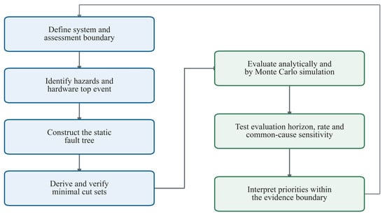
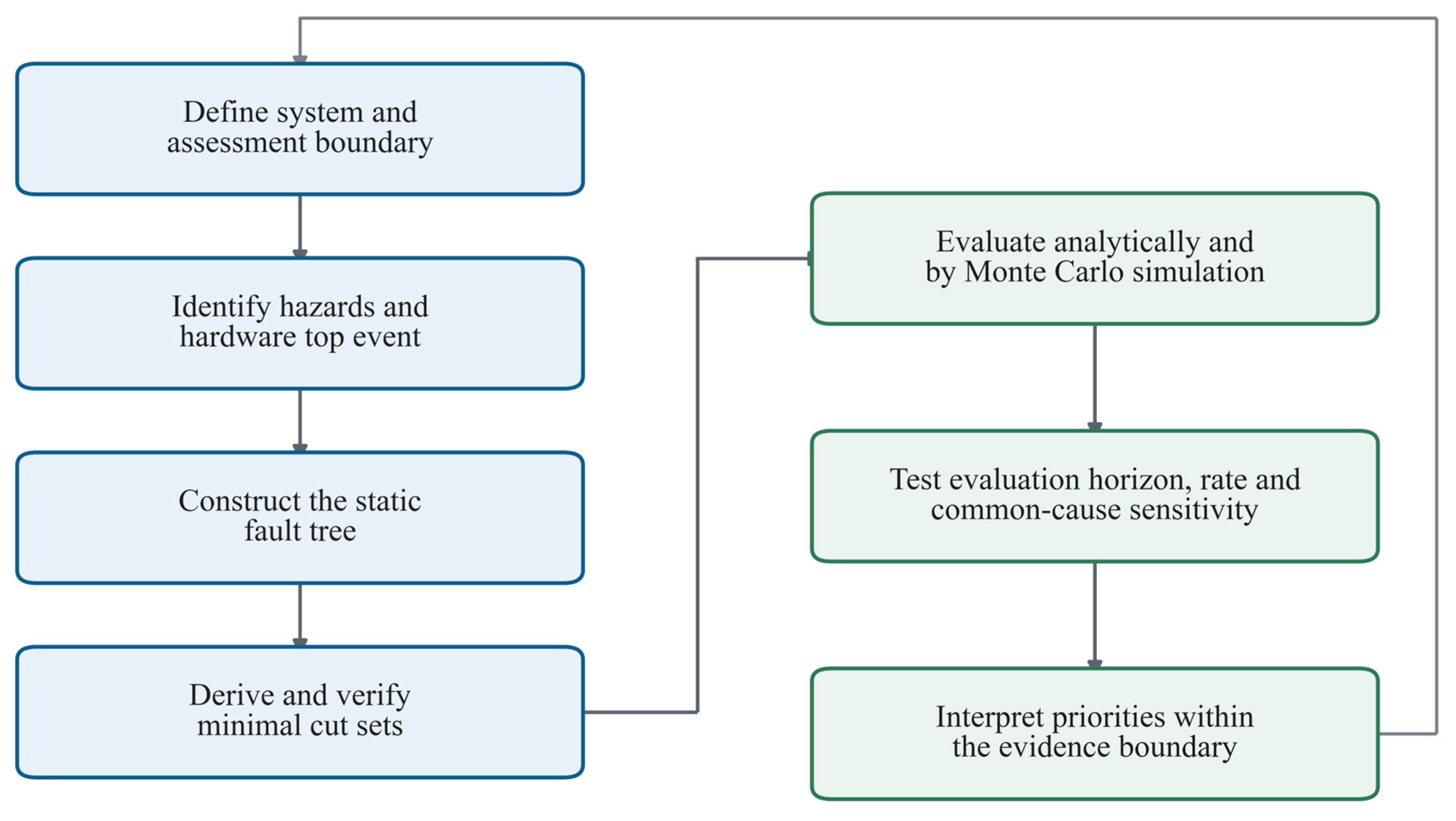
Figure 1 summarizes the analysis process for ground-impact hazards: failure-mode and hazardous-event identification, fault-tree construction, and result evaluation. The workflow is applied to the UAS case study described below.

Figure 1. Evidence-bounded workflow for the UAS hardware fault-tree assessment.

4. Case Study: Solar-Powered UAS

Ground-impact hazards are considered from aircraft start-up through shutdown after landing and comprise the following accident types:

• Damage during taxiing. During take-off, operator error or airframe failure may cause the UAV to leave the intended path, including runway excursions and overturning following a tyre failure.
• Loss of control during flight. Failures of the flight management system, data link or other systems may cause the UAV to lose control and strike the ground.
• Damage during landing. A UAV may land outside the runway, leave the runway or overturn because of landing gear failure or a flat tyre.

In-flight loss of control is selected because the represented power, flight-management and communication functions define a common hardware top event for comparing component priorities. Taxiing and landing additionally require phase-specific gear, runway and operating models and remain in the qualitative hazard inventory.

4.1. System Description and Disclosed Configuration

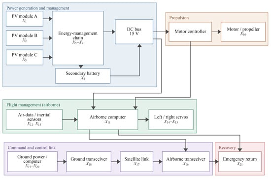
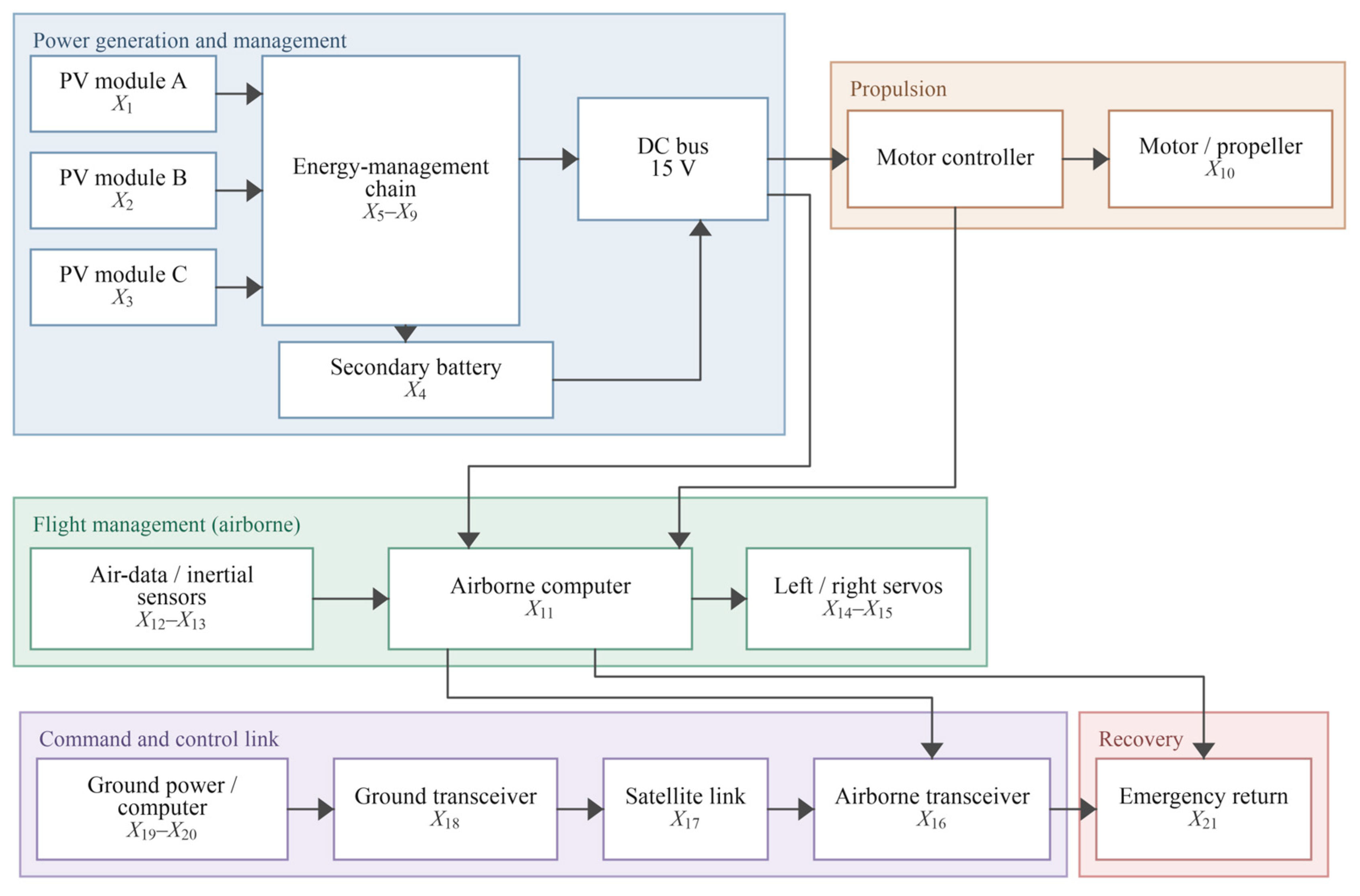
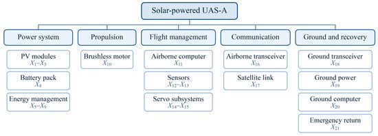
The anonymized case-study platform is denoted UAS-A. The disclosed configuration comprises a 15 kg take-off mass, a maximum cruise speed of 54 km/h, three parallel PV modules, a secondary battery, a 15 V DC bus, a brushless-motor propulsion path, a triple-redundancy airborne-computer subsystem, flight-state sensors, two non-interchangeable servo channels, airborne and ground links, and an emergency-return function. The reference fault tree represents three parallel PV modules and a series battery function; the engineering conditions for this abstraction are considered in Section 5.1. Figure 2 maps these functions to the 21 basic events, providing the basis for the subsequent fault-tree analysis.

Figure 2. Functional architecture and basic-event mapping of UAS-A.

The 24 h interval is a one-day reference evaluation horizon, selected as a representative point within the 1–48 h short-horizon comparison. Its interpretation concerns reliability-metric comparison; a feasible flight duration depends on the operating profile and energy budget. The 8760 h point provides a one-year reference, and 40,000 h samples the region near the model’s mean lifetime. These longer horizons describe failure accumulation in the non-repairable model. Section 6.6 reports the short-horizon ranking check.

4.2. Hazard Identification and Quantitative Boundary

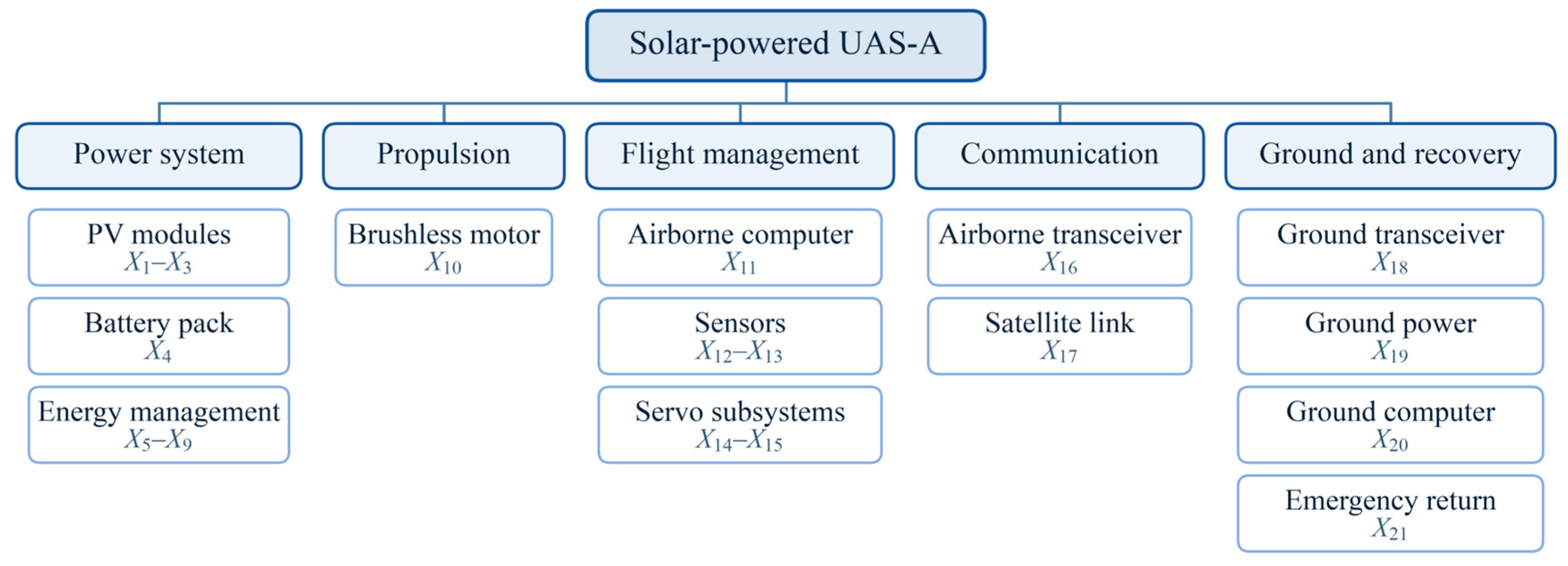
For the failure and effects analysis, the system boundaries and level of detail must be specified. The initial level is the UAV system, and the lowest level comprises its subsystems and actuating devices. The system hierarchy is shown in Figure 3.

Figure 3. System hierarchy used to define the 21 basic events.

Table 1 separates a general hazard inventory from the hardware events quantified for UAS-A. Across these loss-of-control hazards, the subsequent events are generally characterized by unpredictable flight paths, unstable control responses, or uncontrolled descent to the ground. These events may consequently result in collisions with manned aircraft or buildings, ground impact causing injury or death, wreckage or debris hazards, and post-impact fire or explosion. Weather, birds, electromagnetic interference, software, human action, impact exposure, and consequence severity remain qualitative boundary conditions.

Table 1. Loss-of-control hazards and their possible causes during UAV flight.

Hazardous Conditions	Possible Cause
Loss of thrust	(1) Brushless motor or motor-controller failure; (2) Electrical energy depletion; (3) Icing or precipitation; (4) Bird strike
Loss of lift	(1) Structural failure; (2) Weather conditions such as icing and precipitation
Loss of heading, attitude and position information	(1) Fault in heading/attitude system; (2) Fault in navigation system; (3) Insufficient sensing capability of visual perception system in low visibility conditions
Loss of Command/Control Link	(1) Electromagnetic interference; (2) Over-distance flight; (3) Obstruction of antenna; (4) Ground station/control box failure; (5) Unexpected interruption of autopilot; (6) Loss of satellite link
Loss of controller performance	(1) Servo failure; (2) Autopilot failure; (3) Icing or damaged control surfaces
Loss of power system	(1) PV, converter, bus or wiring failure; (2) Secondary-battery or battery-management failure; (3) Energy-management or protection failure
Loss of ground station	(1) Damage to the ground station energy system; (2) Failure of the ground station transmitter/receiver/antenna; (3) Failure of the ground station control computer

5. Fault-Tree Model

5.1. Fault-Tree Construction

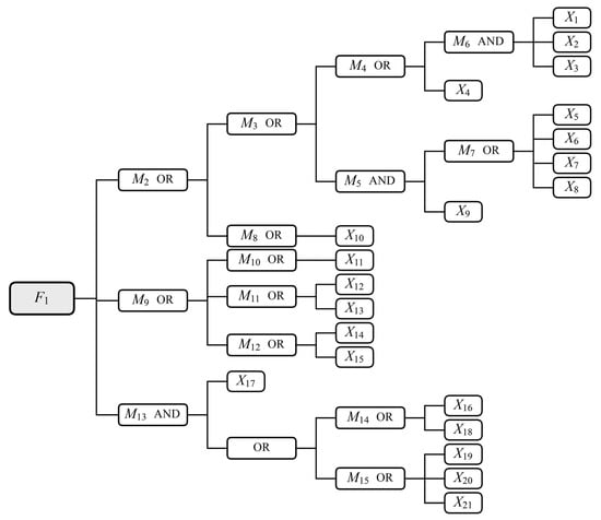
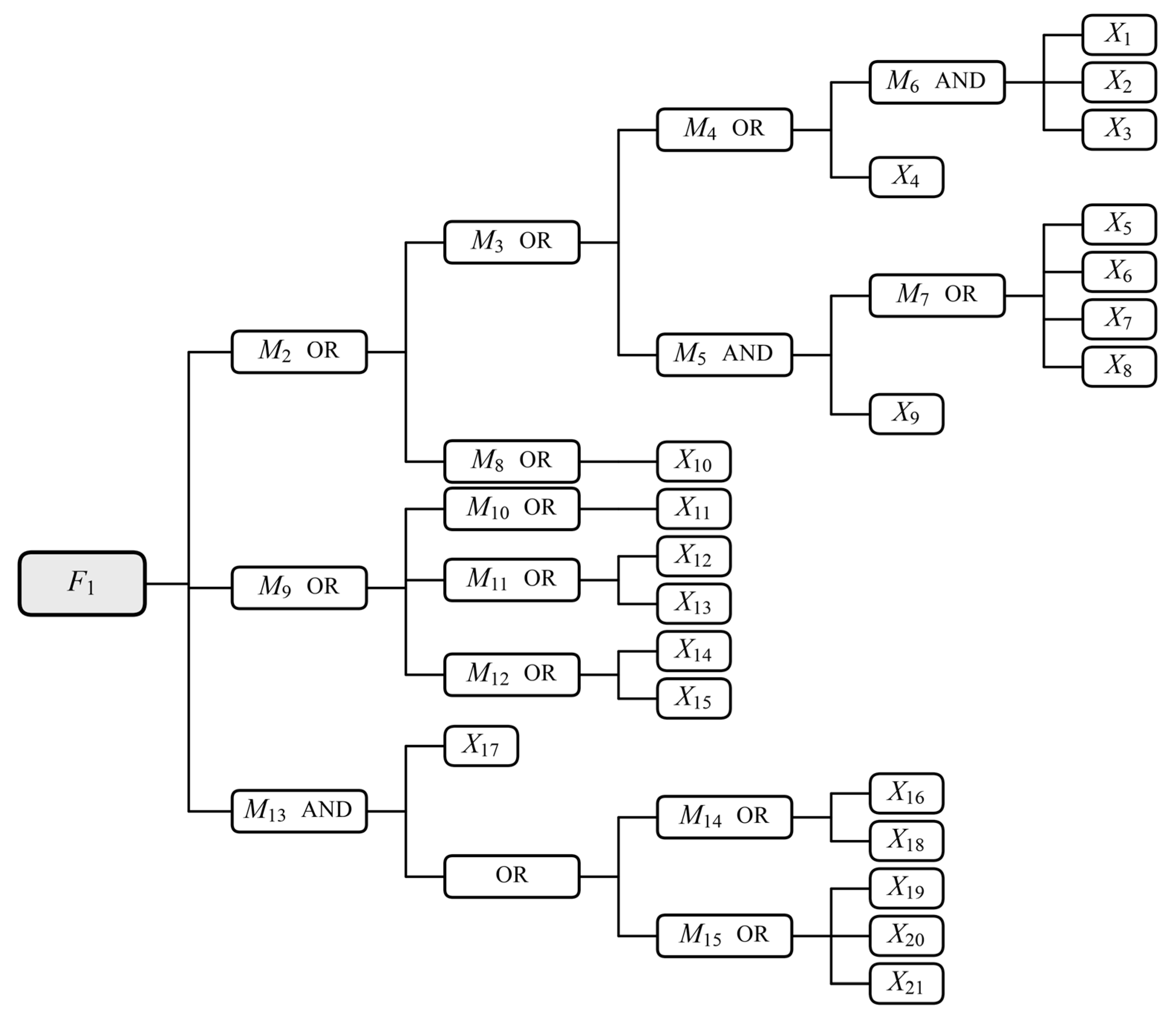
Figure 4 represents hardware-induced loss of control with potential ground impact through specified functional-loss criteria. The baseline assumes permanent, non-repairable and independent failures of 21 basic events. In Equations (1) and (2), either total PV loss or battery failure triggers the power-supply branch. Mapping this battery criterion to the aircraft requires evidence that X₄ propagates to the bus or removes an indispensable supply or control function even with PV available. Battery isolation and continued PV supply would support alternative logic. The two servos retain separate functional paths, and X₁₁ represents the aggregate computer subsystem.

Figure 4. Fault tree for hardware-induced UAV loss of control.

The event symbols and gate types used in the fault tree are defined in Table 2; Supplementary Note S3 maps each gate to its encoded system function.

Table 2. Definition of the various types of events in the UAV fault tree.

Event	Definition	Event Type	Event	Definition	Event Type
F1	Hardware-induced loss of control	Top event	X4	Battery pack failure	Basic event
M2	UAV loss of power	Intermediate events	X5	Voltage detection module fault	Basic event
M3	Loss of power supply system function	Intermediate events	X6	Current detection module fault	Basic event
M4	Power supply system fault	Intermediate events	X7	Temperature detection module fault	Basic event
M5	Power management system fault	Intermediate events	X8	Output control module fault	Basic event
M6	Energy harvester failure	Intermediate events	X9	Power protection module fault	Basic event
M7	Energy data collection and processing module failure	Intermediate events	X10	Loss of motor function	Basic event
M8	Loss of powertrain function	Intermediate events	X11	Triple redundancy airborne computer failure	Basic event
M9	Flight management system failure	Intermediate events	X12	Atmospheric measurement sensor failure	Basic event
M10	Flight control and calculation subsystem failure	Intermediate events	X13	Inertial measurement sensor failure	Basic event
M11	Unable to obtain flight status information	Intermediate events	X14	Left servo subsystem failure	Basic event
M12	Servo system failure	Intermediate events	X15	Right servo subsystem failure	Basic event
M13	UAV link loss	Intermediate events	X16	Airborne Transmitter & Receiver fault	Basic event
M14	UAV unable to receive valid command	Intermediate events	X17	Satellite link lost	Basic event
M15	Ground-control or return-function unavailability	Intermediate events	X18	Ground Station Transmitter & Receiver fault	Basic event
X1	PV module A fault	Basic event	X19	Ground station power supply system fault	Basic event
X2	PV module B fault	Basic event	X20	Ground station control computer fault	Basic event
X3	PV module C fault	Basic event	X21	Emergency return system failure	Basic event

M₁₅ groups ground-power X₁₉, ground-computer X₂₀ and emergency-return X₂₁ failures. Combined with satellite-link loss X₁₇ in Equation (4), the retained OR logic triggers when either the ground-control path or return hardware is unavailable. If either remaining path can independently maintain control or achieve recovery, this trigger overstates physical loss of control. Supplementary Note S2 provides a functional-state table separating the Boolean trigger from the remaining recovery paths. This criterion should be interpreted against the aircraft’s control, switching and recovery requirements.

5.2. Qualitative Analysis and Minimal Cut Sets

An analysis of the UAV loss-of-control event fault tree using the upstream method is shown in the following steps.

Bottom level:

M₆ = X₁ ∩ X₂ ∩ X₃,  M₇ = X₅ ∪ X₆ ∪ X₇ ∪ X₈

(1)

Fourth level:

M₄ = M₆ ∪ X₄,  M₅ = M₇ ∩ X₉

(2)

Third level:

$$\begin{array}{l}{M}_3=M_4\cup M_5,\hspace{1em}{M}_8=X_{10},\hspace{1em}{M}_{10}=X_{11},\hspace{1em}{M}_{11}=X_{12}\cup X_{13},\\ M_{12}=X_{14}\cup X_{15},\hspace{1em}{M}_{14}=X_{16}\cup X_{18},\hspace{1em}{M}_{15}=X_{19}\cup X_{20}\cup X_{21}.\end{array}$$

(3)

Second level:

$$\begin{array}{l}{M}_2=M_3\cup M_8,\hspace{1em}\hspace{1em}{M}_9=M_{10}\cup M_{11}\cup M_{12},\\ M_{13}=X_{17}\cap \left(M_{14}\cup M_{15}\right).\end{array}$$

(4)

First level:

$$\begin{array}{l}\begin{array}{lll}{F}_1\hfill & =M_2\cup M_9\cup M_{13}\hfill & \hfill \\ \hfill & =M_3\cup M_8\cup M_{10}\cup M_{11}\cup M_{12}\cup [X_{17}\cap (M_{14}\cup M_{15})]\hfill & \hfill \\ \hfill & =M_4\cup M_5\cup X_{10}\cup X_{11}\cup X_{12}\cup X_{13}\cup X_{14}\cup X_{15}\hfill & \hfill \end{array}\\ \begin{array}{lll}\hfill & \cup [X_{17}\cap (X_{16}\cup X_{18}\cup X_{19}\cup X_{20}\cup X_{21})]\hfill & \hfill \\ F_1\hfill & =(M_6\cup X_4)\cup (M_7\cap X_9)\cup X_{10}\cup X_{11}\cup X_{12}\cup X_{13}\cup X_{14}\cup X_{15}\hfill & \hfill \\ \hfill & \cup [X_{17}\cap (X_{16}\cup X_{18}\cup X_{19}\cup X_{20}\cup X_{21})]\hfill & \hfill \end{array}\end{array}$$

(5)

Simplified and available:

$$\begin{array}{lll}{F}_1\hfill & =[(X_1\cap X_2\cap X_3)\cup X_4]\cup [(X_5\cup X_6\cup X_7\cup X_8)\cap X_9]\hfill & \hfill \\ \hfill & \cup X_{10}\cup X_{11}\cup X_{12}\cup X_{13}\cup X_{14}\cup X_{15}\hfill & \hfill \\ \hfill & \cup [X_{17}\cap (X_{16}\cup X_{18}\cup X_{19}\cup X_{20}\cup X_{21})]\hfill & \hfill \end{array}$$

(6)

The Boolean expression in Equation (6) yields 17 minimal cut sets:

$$\begin{array}{lll}\hfill & \{X_1,X_2,X_3\},\left\{X_4\right\},\{X_5,X_9\},\{X_6,X_9\},\{X_7,X_9\},.\hfill & \hfill \\ \hfill & \{X_8,X_9\},\left\{X_{10}\right\},\left\{X_{11}\right\},\left\{X_{12}\right\},\left\{X_{13}\right\},\left\{X_{14}\right\},\hfill & \hfill \\ \hfill & \begin{array}{l}\left\{X_{15}\right\},\{X_{16},X_{17}\},\{X_{18},X_{17}\},\{X_{19},X_{17}\},\\ \{X_{20},X_{17}\},\{X_{21},X_{17}\}\end{array}\hfill & \hfill \end{array}$$

(7)

There are seven first-order, nine second-order and one third-order minimal cut sets. First-order minimal cut sets account for 41.2% of the total. The gates in Figure 4 and Equations (1)–(6) are consistent with these 17 sets.

6. Quantitative Reliability Assessment

6.1. System Simulation Model

Assuming that a UAS consists of n basic components, it can be expressed as

S = {X₁,X₂,…,X_i,…,X_n}

(8)

where X_i (i = 1, 2, …, n) denotes a basic component and, in the fault tree, its failure event. Its failure distribution function is F_i(t).

The fault tree reflects the logical relationship between the top and basic events. The top event F₁ represents failure of system S under the stated model assumptions.

The binary variable x_i(t) represents the failure state of basic event i at time t:

$$x_i(t)=\left\{\begin{array}{ll}1,\hfill & \mathrm{if}\mathrm{event}i\mathrm{has}\mathrm{occurred}\mathrm{by}t,\hfill \\ 0,\hfill & \mathrm{otherwise}.\hfill \end{array}\right.$$

(9)

Similarly, the state of the top event F₁ at time t is represented by ϕ(x(t)), where x(t) = (x₁(t), …, x_n(t)):

$$\varphi \left(x(t)\right)=\left\{\begin{array}{ll}1,\hfill & \mathrm{if}\mathrm{the}\mathrm{top}\mathrm{event}\mathrm{has}\mathrm{occurred}\mathrm{by}t,\hfill \\ 0,\hfill & \mathrm{otherwise}.\hfill \end{array}\right.$$

(10)

The top-event state is fully determined by the vector of basic-event states.

For a fault tree with k minimal cut sets, let C_a be the component-index set of cut set a. Its failure indicator is K_a(x) = ∏_l∈Cax_l. The structure function is

$$\varphi (x)=1-{\displaystyle {\displaystyle \prod _{a=1}^k}\left(1-{\displaystyle \prod _{l\in C_a}{x}_l}\right)}$$

(11)

Since ϕ(x(t)) takes values of zero or one, the top-event probability F_s(t) is

F_s(t) = E [ϕ (x(t))] = P {ϕ (x(t)) = 1}

(12)

6.2. Lifetime Sampling and Event Ordering

In each simulation, the lifetimes of the n basic components are sampled independently by the Monte Carlo method.

Let t_ij denote the failure time of component i in trial j. Inverse-transform sampling gives

$$t_{\mathit{ij}}=F_i^{-1}\left({\eta }_{\mathit{ij}}\right)$$

(13)

where η_ij is an independent uniform random variable on (0, 1). For the constant failure rates λ_i used here, F_i(t) = 1 − e^−λ_i^t and t_ij = −ln(1 − η_ij)/λ_i.

According to Equations (9) and (13), the component state in trial j is

$$x_{\mathit{ij}}(t)=\left\{\begin{array}{ll}1,\hfill & t\ge t_{\mathit{ij}},\hfill \\ 0,\hfill & t<t_{\mathit{ij}}.\hfill \end{array}\right.$$

(14)

The component states determine the state of system S. Let τ_j be the system failure time in trial j. Then

$${\varphi }_j(t)=\left\{\begin{array}{ll}1,\hfill & t\ge {\tau }_j,\hfill \\ 0,\hfill & t<{\tau }_j.\hfill \end{array}\right.$$

(15)

To find τ_j, sort the component failure times in trial j from smallest to largest: t_(1)j, t_(2)j, …, t_(n)j. Let f_r identify the component with the r-th ordered failure time.

Start with all components functioning. At t_(1)j, set component X_f1 to the failed state and evaluate the fault tree. If the top event has not occurred, retain this failed state and continue through the ordered component failures. The first index r_j for which the top event occurs gives τ_j = t_(rj)j. The trial then ends.

Equation (15) can therefore be written as

$${\varphi }_j(t)=\left\{\begin{array}{ll}1,\hfill & t\ge {\tau }_j=t_{(r_j)j},\hfill \\ 0,\hfill & t<{\tau }_j=t_{(r_j)j}.\hfill \end{array}\right.$$

(16)

The system failure distribution is estimated from N trials. The display horizon T_max is divided into m intervals. Every trial is simulated to system failure, including failures beyond the display horizon. The number of failures in (t_r−1, t_r] is defined below.

Here, 1{A} equals one if condition A holds and zero otherwise.

$$\Delta m_r={\displaystyle \sum _{j=1}^{N}1}\left\{t_{r-1}<{\tau }_j\le t_r\right\}$$

(17)

The number of system failures by time t_r is

$$m_r={\displaystyle \sum _{j=1}^{N}1}\left\{{\tau }_j\le t_r\right\}$$

(18)

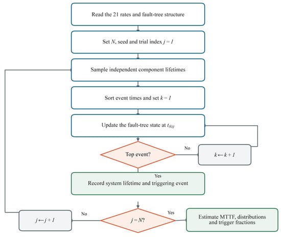
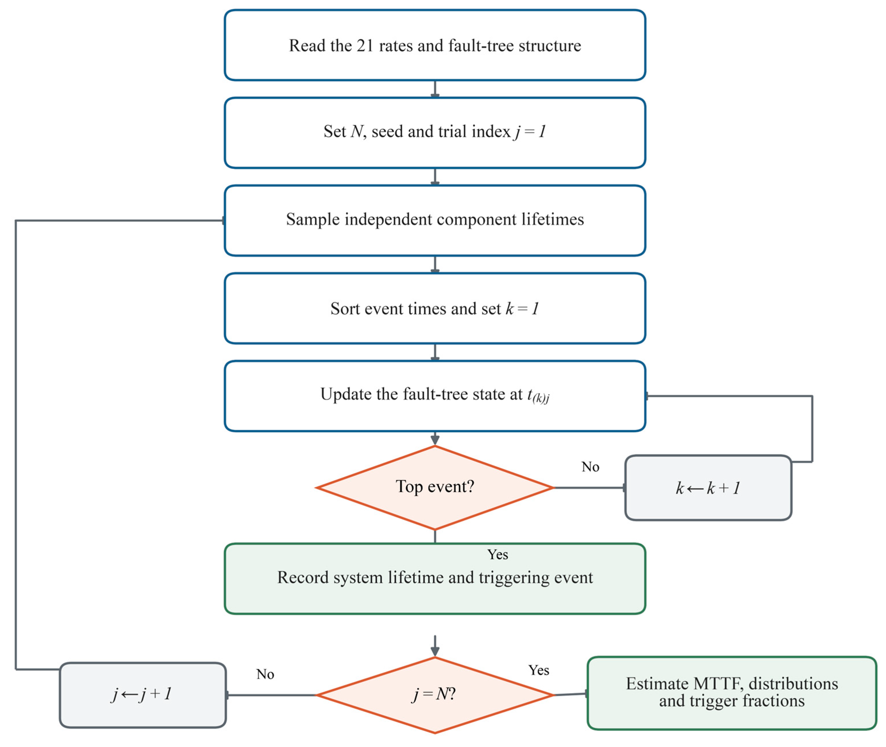
The numerical implementation follows the event-order procedure described above. For each trial, component lifetimes are sampled independently, ordered chronologically, and applied sequentially to the fault-tree state until the top event is first triggered. The resulting system lifetime and triggering event are then recorded. Python and MATLAB implement this procedure independently using separate random-number generators, while an exact analytical recursion and exhaustive Boolean-state tests are used to cross-check the fault-tree logic and first-trigger bookkeeping. A static Simulink model provides an additional check of the gate topology. The overall simulation sequence is summarized in Figure 5.

Figure 5. Flow chart of the UAV safety analysis simulation programme.

6.3. Reliability and Finite-Horizon Metrics

Let ξ denote the system lifetime. Its cumulative distribution function F_s(t) is estimated as

$$F_{\mathrm{s}}(t_r)=\mathrm{P}(\xi \le t_r)\approx {\displaystyle \frac{1}{N}}{\displaystyle \sum _{j=1}^N{\varphi }_j}(t_r)$$

(19)

Combining Equations (18) and (19) gives

$$F_{\mathrm{s}}(t_r)\approx {\displaystyle \frac{m_r}{N}}$$

(20)

The failure probability mass P_s,r for interval (t_r−1, t_r] is

$$P_{\mathrm{s},r}=\mathrm{P}(t_{r-1}<\xi \le t_r)\approx {\displaystyle \frac{1}{N}}{\displaystyle \sum _{j=1}^{N}1}\left\{t_{r-1}<{\tau }_j\le t_r\right\}$$

(21)

Combining Equations (17) and (21) gives

$$P_{\mathrm{s},r}=F_{\mathrm{s}}(t_r)-F_{\mathrm{s}}(t_{r-1})\approx {\displaystyle \frac{\Delta m_r}{N}}$$

(22)

The density histogram uses Δm_r/[N(t_r − t_r−1)], with units of h⁻¹. For the non-repairable system, the mean lifetime is the mean time to first failure (MTTF), estimated from all sampled lifetimes:

$$\mathrm{MTTF}=\mathrm{E}(\xi )={\displaystyle {\int }_0^{\infty }{R}_{\mathrm{s}}}(t)\mathrm{d}t\approx {\displaystyle \frac{1}{N}}{\displaystyle {\displaystyle \sum _{j=1}^N}{\tau }_j}$$

(23)

The instantaneous hazard is h_s(t) = f_s(t)/R_s(t) = −d ln R_s(t)/dt for R_s(t) > 0, where f_s(t) = dF_s(t)/dt is the system failure density. It gives the conditional failure rate among systems surviving to t and can vary even when all component rates are constant. The reciprocal of MTTF provides a descriptive inverse-lifetime scale, while F_s(T_m)/T_m is the average cumulative top-event probability per unit time. Finite-horizon hardware screening compares F_s(T_m) with an assumed rate ceiling, ρ_T, converted to a finite-horizon probability as follows:

F_s(T_m) = 1 − R_s(T_m) ≤ ρ_TT_m

(24)

For component X_i, let A_i be the number of trials in which its failure triggers the first system failure, and let B_i be the number of trials in which it has failed by the system stopping time. The conditional trigger fraction (CTF) is

$$\mathrm{CTF}(X_i)={\displaystyle \frac{A_i}{B_i}}$$

(25)

The trigger share (TS) is defined below. Together, CTF and TS provide event-order attribution measures, whereas Birnbaum, Fussell–Vesely, risk achievement worth (RAW) and risk reduction worth (RRW) represent different importance concepts. With continuous lifetimes, one component triggers each baseline trial, so ∑_iA_i = N, ∑_iTS(X_i) = 1 and CTF(X_i) ≥ TS(X_i).

$$\mathrm{TS}(X_i)={\displaystyle \frac{A_i}{N}}$$

(26)

6.4. Failure-Rate Inputs and Common-Cause Scenarios

Table 3 gives the component and subsystem failure-rate inputs compiled with reference to NPRD-2023, EPRD-2024, SAE ARP5890B, MIL-HDBK-217F Notice 2 and related standards, together with experimental results [29,30,34,35]. X₁₁ is represented by an aggregate subsystem rate. The same values are used in the analytical and simulation models; rate perturbations and PV scans characterize sensitivity around this baseline.

Table 3. Component and subsystem failure-rate inputs.

Event	Subsystem/Device	Rate (10−6 h−1)
X1	PV module A	31
X2	PV module B	31
X3	PV module C	31
X4	Battery pack	1.2
X5	Voltage detection module	6.5
X6	Current detection module	6.5
X7	Temperature detection module	6.5
X8	Output control module	6.5
X9	Power protection module	5.5
X10	Brushless motor	0.2
X11	Triple-redundancy airborne computer	0.3
X12	Atmospheric measurement sensor	0.3
X13	Inertial measurement sensor	0.3
X14	Left servo subsystem	0.8
X15	Right servo subsystem	0.8
X16	Airborne transmitter and receiver	3.3
X17	Satellite link	1.8
X18	Ground transmitter and receiver	3.3
X19	Ground station power supply	2.5
X20	Ground station control computer	6.5
X21	Emergency return system	6.5

Note: The 21 failure-rate values were compiled with reference to NPRD-2023, EPRD-2024, SAE ARP5890B, MIL-HDBK-217F Notice 2 and related standards, together with experimental results [29,30,34,35].

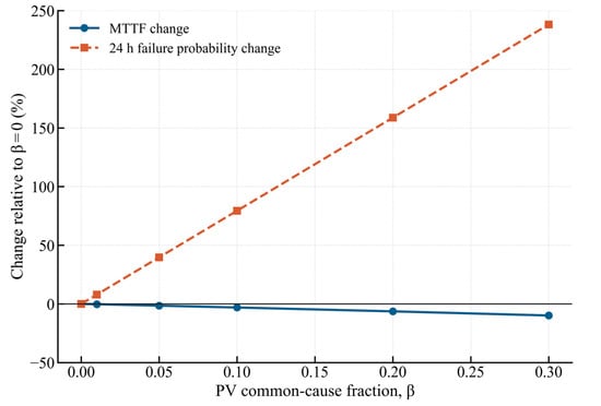
The disclosed architecture identifies the three PV modules as functionally interchangeable; accordingly, the supplementary β-factor scenario partitions each baseline PV rate into an independent part and a common-cause event. The baseline remains β = 0 and keeps its 21 events and 17 cut sets. For β > 0,

λ_PV,I = (1 − β)λ_PV,  λ_PV,C = βλ_PV

(27)

The common event is independent of the residual module-specific processes and adds a first-order PV failure path. The sensitivity points are β ∈ {0.01,0.05,0.1,0.2,0.3}. Analogous shocks are evaluated for the servo and transceiver pairs, separately and jointly with PV, while preserving marginal rates. Both pairs occupy OR failure gates in the present tree. X₁₁ remains an aggregate event whose total rate is varied by factors of 0.5, 1.5 and 2; decomposition requires channel and voter data. Supplementary Note S1 specifies these checks. Note S2 tests PV dependence across horizons using 19 intervention targets: the PV group and the other 18 events. At fixed β, a PV-rate perturbation scales both the shared and residual rates together.

6.5. Baseline Lifetime and Finite-Horizon Results

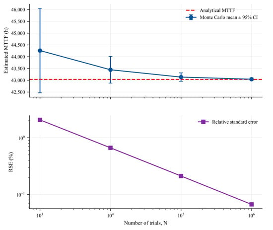
The Python simulation gives an MTTF of 43,045.3 h (95% Monte Carlo interval 42,989.0–43,101.6 h), the MATLAB estimate is 43,030.8 h, and the analytical value is 43,038.8 h. The close agreement among the analytical, Python, and MATLAB calculations supports implementation consistency of the stated fault-tree model. Validation of the functional topology and predicted service lifetime requires independent platform-level evidence. The N = 10³ to 10⁶ convergence study shows the Monte Carlo relative standard error declining approximately with N^−1/2 to 0.067% at one million trials.

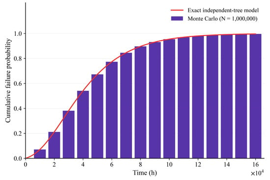
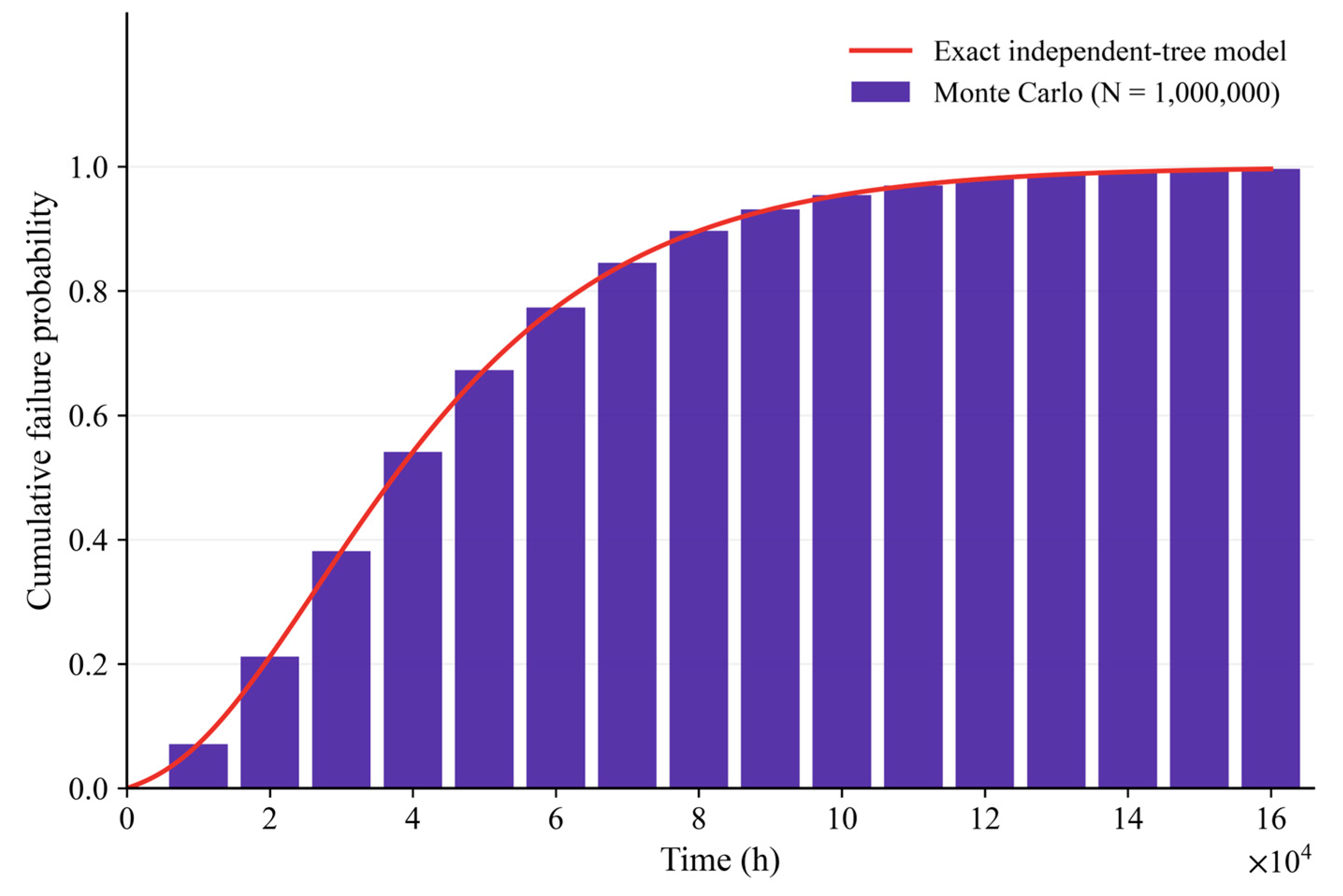
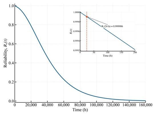
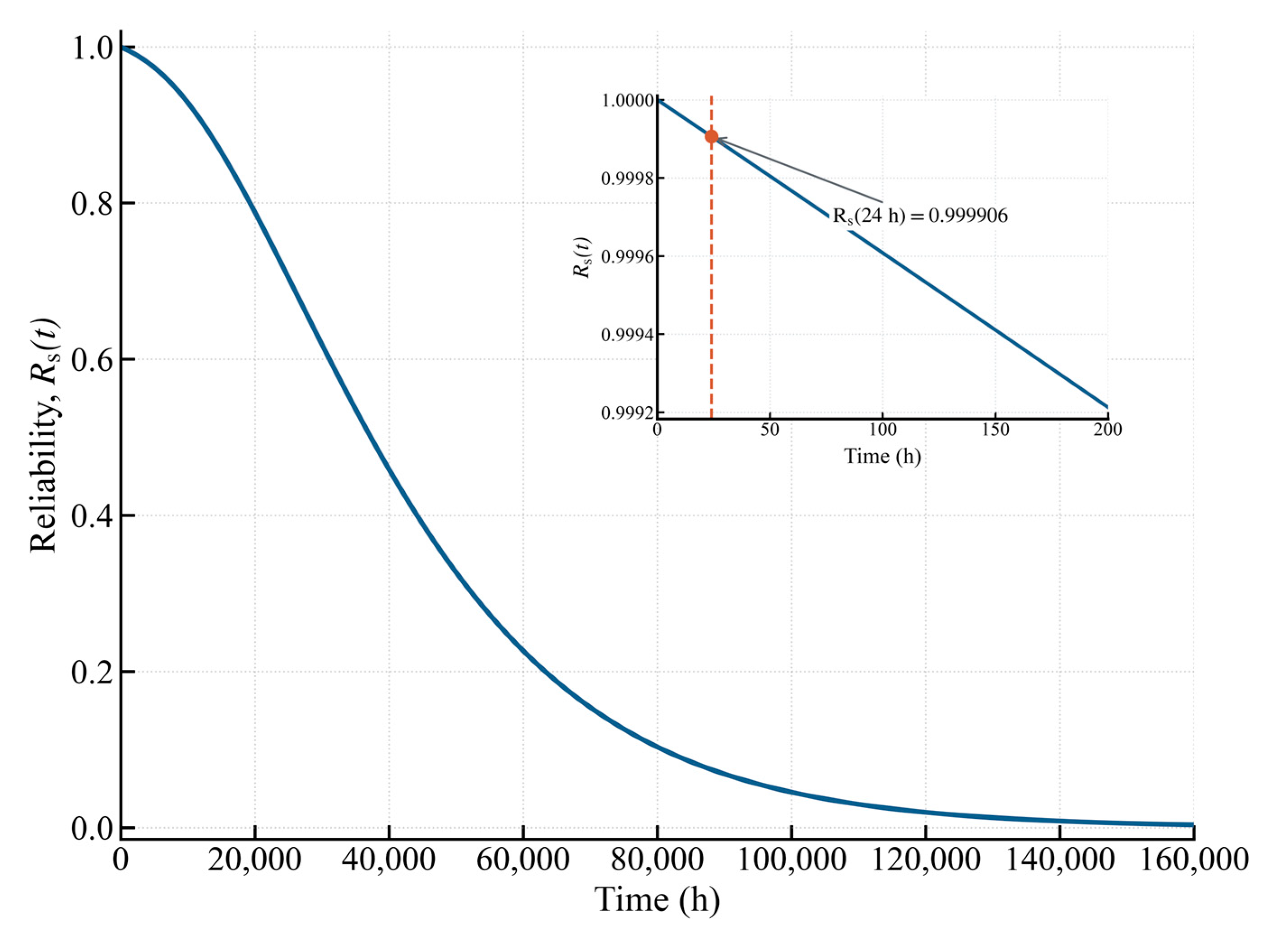
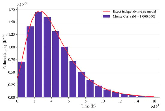
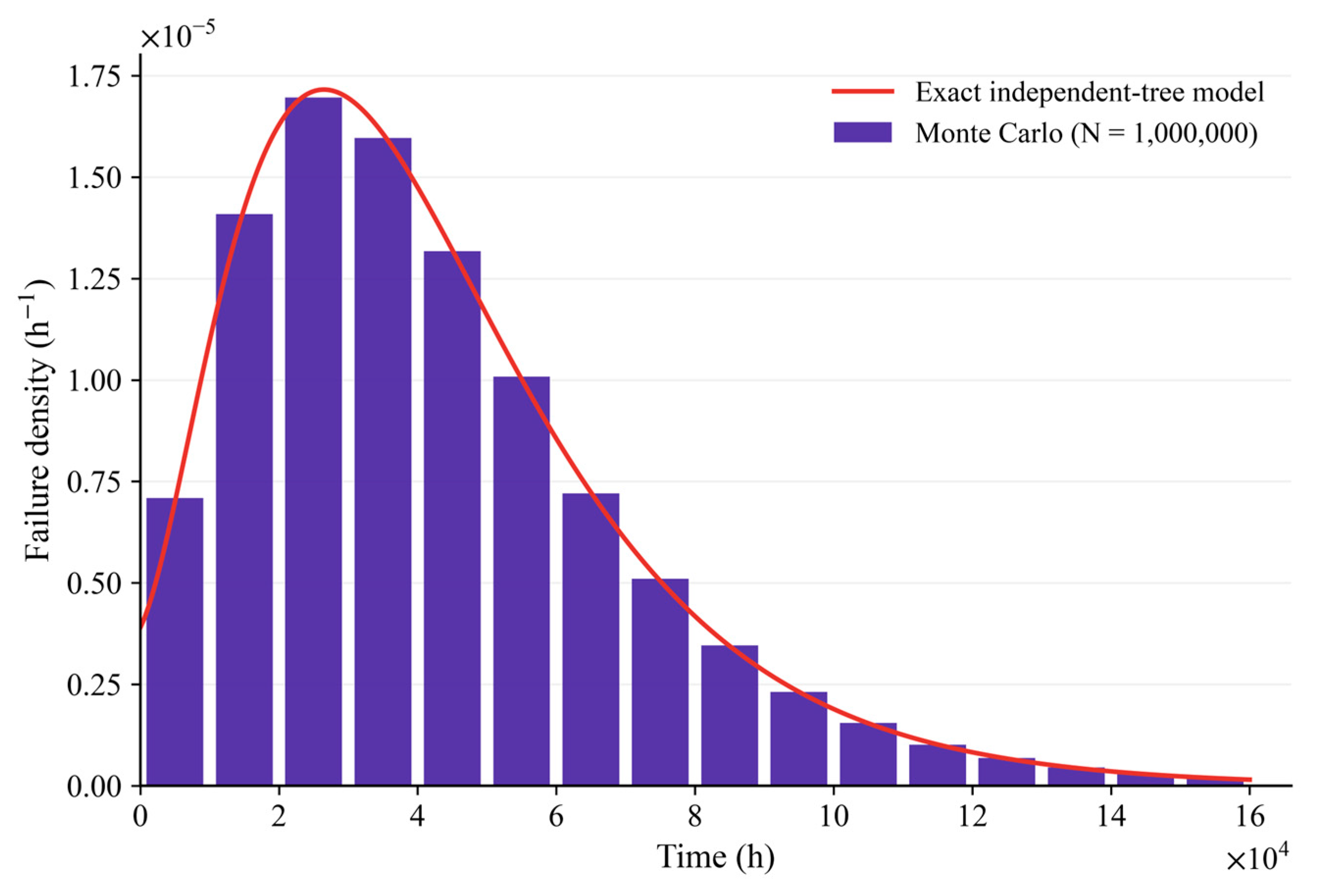
With T_m = 24 h adopted as the reference horizon, the independent analytical baseline gives F_s(T_m) = 9.3701 × 10⁻⁵, R_s(T_m) = 0.9999063, and F_s(T_m)/T_m = 3.9042×10⁻⁶ h⁻¹. The instantaneous hazard is h_s(24 h) = 3.9088 × 10⁻⁶ h⁻¹, compared with 1/MTTF = 2.3235 × 10⁻⁵ h⁻¹. This top-event probability is below the illustrative finite-horizon ceilings obtained from 10⁻⁴ h⁻¹ and 10⁻⁵ h⁻¹, whose 24 h values are 2.4 × 10⁻³ and 2.4 × 10⁻⁴. This screening margin applies to the independent baseline and the assumed ceilings. Airworthiness, ground-impact frequency, and casualty risk require the broader operational evidence described in Section 2.1. Figure 6 presents the cumulative failure distribution, Figure 7 gives the analytical reliability curve with the 24 h inset, and Figure 8 shows the corresponding failure density.

Figure 6. Cumulative failure distribution of the UAS.

Figure 7. Analytical system reliability with the 24 h reference evaluation horizon shown in the inset.

Figure 8. Failure density of the UAS.

The CTF and TS measures identify which component first makes the static top event true in each simulated lifetime. Table 4 reports Monte Carlo attribution values, ranked by TS. For X₄ and X₁₀–X₁₅, CTF = 1 follows exactly from their singleton cut sets: failure of any such event stops the trial, so its counts A_i and B_i coincide. This structural property provides no ordering within that group. TS allocates first-trigger cases for diagnostic and test prioritization; component-improvement choices use the sensitivity of the intended reliability metric.

Table 4. Monte Carlo conditional trigger fraction and trigger share, ranked by TS.

Event	Component	CTF	TS	Rank
X1	PV module A	0.2586	0.2039	2
X2	PV module B	0.2578	0.2034	3
X3	PV module C	0.2585	0.2040	1
X4	Battery pack	1.0000	0.0518	5
X5	Voltage detection module	0.0686	0.0162	9
X6	Current detection module	0.0680	0.0160	12
X7	Temperature detection module	0.0683	0.0160	11
X8	Output control module	0.0686	0.0162	10
X9	Power protection module	0.4644	0.1038	4
X10	Brushless motor	1.0000	0.0087	16
X11	Triple-redundancy airborne computer	1.0000	0.0129	13
X12	Atmospheric measurement sensor	1.0000	0.0128	15
X13	Inertial measurement sensor	1.0000	0.0129	14
X14	Left servo subsystem	1.0000	0.0346	7
X15	Right servo subsystem	1.0000	0.0346	6
X16	Airborne transmitter and receiver	0.0238	0.0031	19
X17	Satellite link	0.4265	0.0323	8
X18	Ground transmitter and receiver	0.0233	0.0030	20
X19	Ground station power supply	0.0231	0.0023	21
X20	Ground station control computer	0.0248	0.0058	18
X21	Emergency return system	0.0250	0.0058	17

The three PV events account for 61.12% of baseline first triggers, conditional on the baseline rate of 31 × 10⁻⁶ h⁻¹ used for each module. The next largest contribution is the power-protection module X₉ (TS = 0.1038). Its role follows from the management branch: when X₉ has failed, any of X₅–X₈ completes a second-order cut set. This identifies X₉ as a long-horizon lifetime-attribution priority.

The emergency-return event X₂₁ has TS = 0.0058 (rank 17 of 21) and appears with satellite-link loss X₁₇ in the cut set {X₁₇, X₂₁}. This rank describes the event’s contribution to the static hardware top event. The safety benefit of successful detection, return activation and recovery is a separate functional outcome, whose assessment requires switching logic, available energy and return-success behaviour. Engineering evaluation of emergency return should include these recovery functions alongside its hardware availability.

6.6. Sensitivity, Common-Cause and Convergence Results

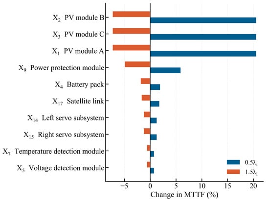
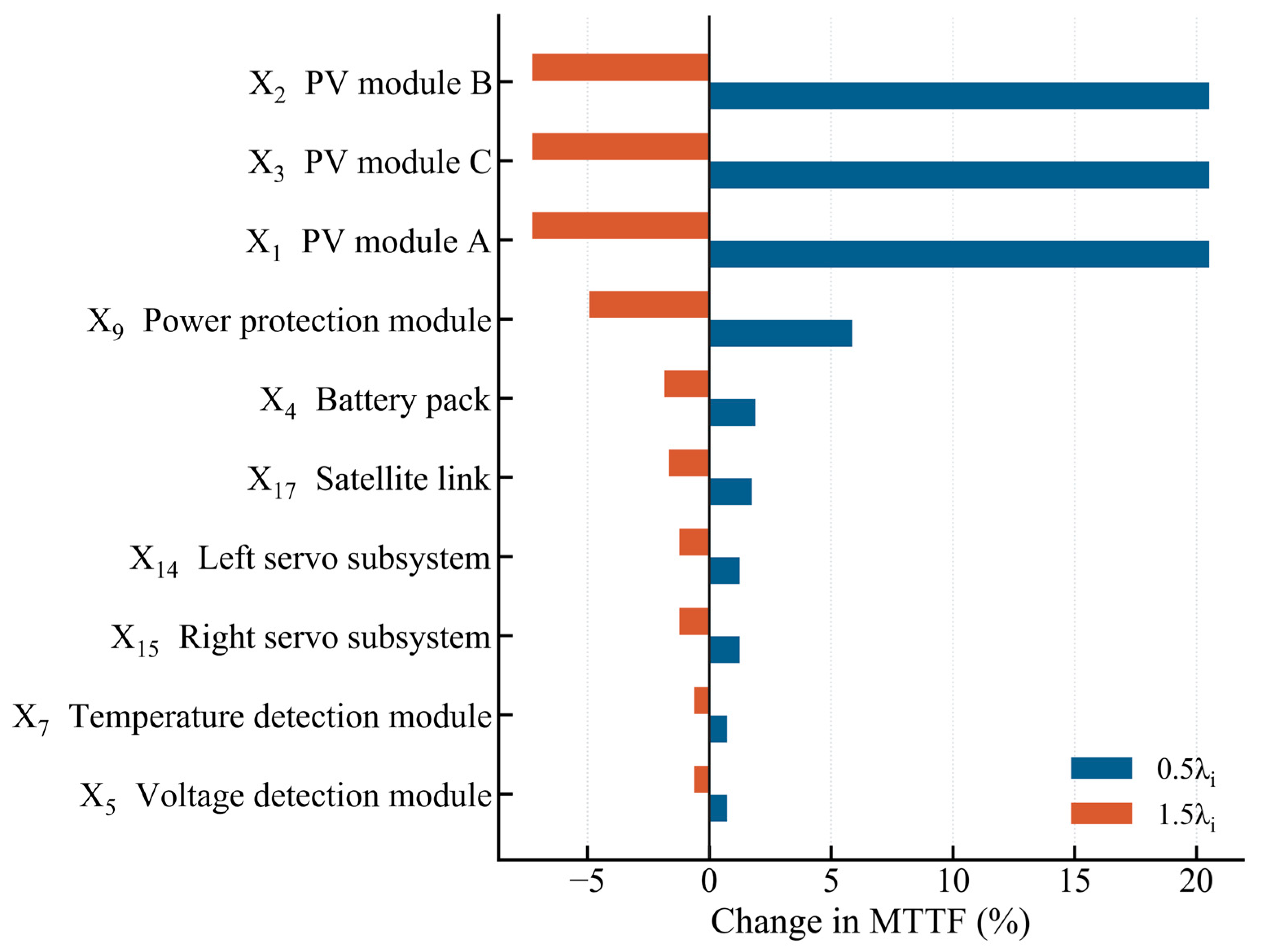
One-at-a-time perturbations (0.1, 0.5, 0.8, 1.2, 1.5 and 10 times each baseline rate) show that MTTF is most sensitive to the three PV inputs, followed by X₉, X₄, X₁₇ and the two servo events. The ±50% tornado plot preserves this lifetime-scale ordering, while the one-order stress cases characterize its wider-range response. The complete 126-scenario table is provided as Supplementary Data S1 (oat_sensitivity.csv). Figure 9 displays the matched ±50% lifetime-scale sensitivities. Across 544 joint background-rate profiles with multipliers between 0.5 and 1.5, the seven first-order events retain the top seven 24 h positions for both perturbation factors, while individual orders and lifetime PV positions vary. Cross-metric correlations range from −0.232 to 0.454; Supplementary Note S3 gives the joint design and results.

Figure 9. One-at-a-time sensitivity of MTTF to ±50% component-rate changes.

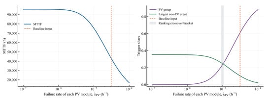
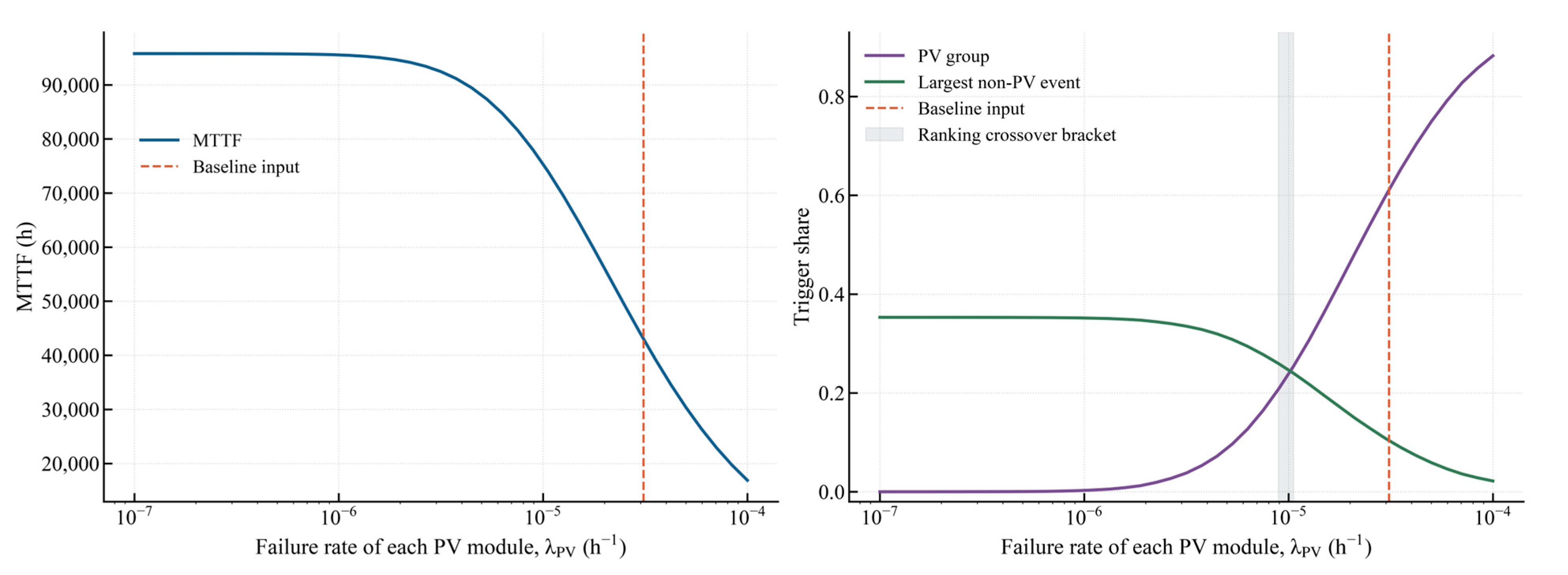
The PV scan brackets the trigger-ranking crossover between 8.91 × 10⁻⁶ and 1.06 × 10⁻⁵ h⁻¹ per module in the common-random-number experiment. Below that interval, the largest non-PV event has a greater trigger share than the combined PV group. The baseline value of 31 × 10⁻⁶ h⁻¹ lies well above the crossover; therefore, PV dominance in the lifetime-trigger ranking depends on the assumed PV rate, whereas the presence of several non-redundant first-order cut sets remains structurally robust. Figure 10 shows the complete rate-dependent MTTF and trigger-share response.

Figure 10. MTTF and trigger-share dependence on the assumed failure rate of each PV module.

At β = 0.1, the PV common-cause scenario gives an MTTF of 41,717 h and F_s(24 h) = 1.6809 × 10⁻⁴. Its common-shock rate, 3.1 × 10⁻⁶ h⁻¹, approaches the combined 3.9 × 10⁻⁶ h⁻¹ rate of the seven baseline first-order paths. In the matched 19-target check, PV moves from rank 19 at β = 0 to rank 1 at β = 0.05 for the 24 h probability sensitivity under a 0.5-rate perturbation. Thus, weak short-horizon PV sensitivity depends on independence. At β = 0.2, F_s(24 h) = 2.42476 × 10⁻⁴ exceeds the illustrative 2.4 × 10⁻⁴ ceiling by 1.03%. Assigning β = 0.1 jointly to PV, servos and transceivers gives 41,831.9 h and 1.6617 × 10⁻⁴: at fixed marginals, shared shocks reduce the union probability at the two OR gates while creating a direct PV failure path. Figure 11 shows the PV scenario; Supplementary Notes S1 and S2 provide the group checks and horizon scans. Aircraft-specific β values require common-event observations.

Figure 11. PV common-cause stress scenario over the assumed β range.

At N = 10⁶, the mean-lifetime estimate has converged, while rare-event counting remains limited by the expected event count. A probability near 10⁻⁵ yields approximately ten events per million trials. Accordingly, finite-horizon probabilities are obtained from the analytical fault-tree solution, with Monte Carlo used for implementation cross-checking and attribution sampling. Figure 12 separates MTTF convergence from the precision limits of rare-event counting.

Figure 12. Monte Carlo convergence of MTTF and relative standard error.

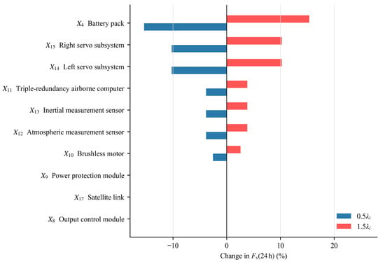
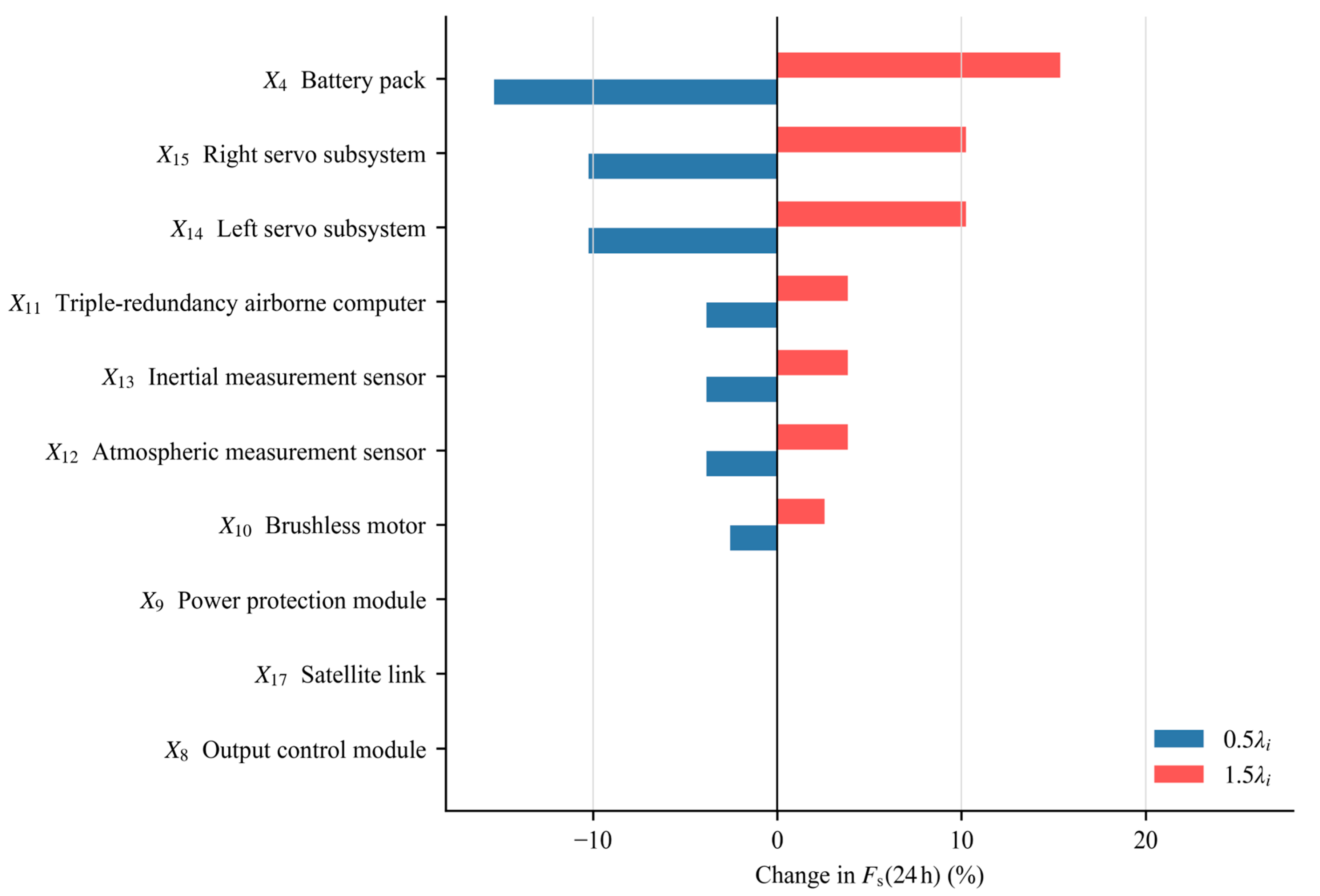
Under independence, the 24 h probability produces a different ranking because first-order cut sets dominate at short duration. Raising one rate by a factor of ten changes F_s(24 h) by +276.6% for the battery X₄, +184.4% for either servo X₁₄ or X₁₅, +69.1% for each airborne-computer/sensor input X₁₁–X₁₃, and +46.1% for the motor X₁₀. At the matched 0.5λ_i perturbation used in Figure 9, the leading finite-horizon order is unchanged: the reductions are 15.37% for X₄, 10.24% for either servo, 3.84% for each of X₁₁–X₁₃ and 2.56% for X₁₀, compared with only 0.044% for X₉ and 0.00022% for each PV module. The matched perturbation confirms the lifetime–finite-horizon ranking contrast under a common amplitude. For independent exponential basic events with λ_it ≪ 1, the probability of a k-event cut set is of order t^k; this suppresses the second- and third-order paths at short evaluation horizons. Figure 13 displays the matched ±50% finite-horizon sensitivity used for the direct ranking comparison.

Figure 13. One-at-a-time sensitivity of the 24 h top-event probability to ±50% component-rate changes.

Table 5 reports the independent-baseline probabilities and screening margins over 1–48 h. At 1, 4, 8, 24 and 48 h, the matched 0.5-rate sensitivity rankings are identical and r_S = 0.054641. The average top-event probability per unit time remains close to 3.9 × 10⁻⁶ h⁻¹, the sum of the rates of the seven first-order cut sets. The margin to the illustrative 10⁻⁵ h⁻¹ ceiling changes from 2.564 to 2.559. The 24 h result therefore represents this sampled short-horizon range. Supplementary Note S2 gives the first-order expansion and numerical checks.

Table 5. Evaluation-horizon dependence of the independent-baseline top-event probability.

Tm (h)	Fs(Tm)	Fs(Tm)/Tm (h−1)	Margin to 10−4 h−1	Margin to 10−5 h−1
1	3.9002 × 10−6	3.9002 × 10−6	25.64	2.564
4	1.5603 × 10−5	3.9007 × 10−6	25.64	2.564
8	3.1211 × 10−5	3.9014 × 10−6	25.63	2.563
24	9.3701 × 10−5	3.9042 × 10−6	25.61	2.561
48	1.8761 × 10−4	3.9085 × 10−6	25.59	2.559

6.7. Lifetime Versus Finite-Horizon Ranking Divergence

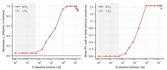
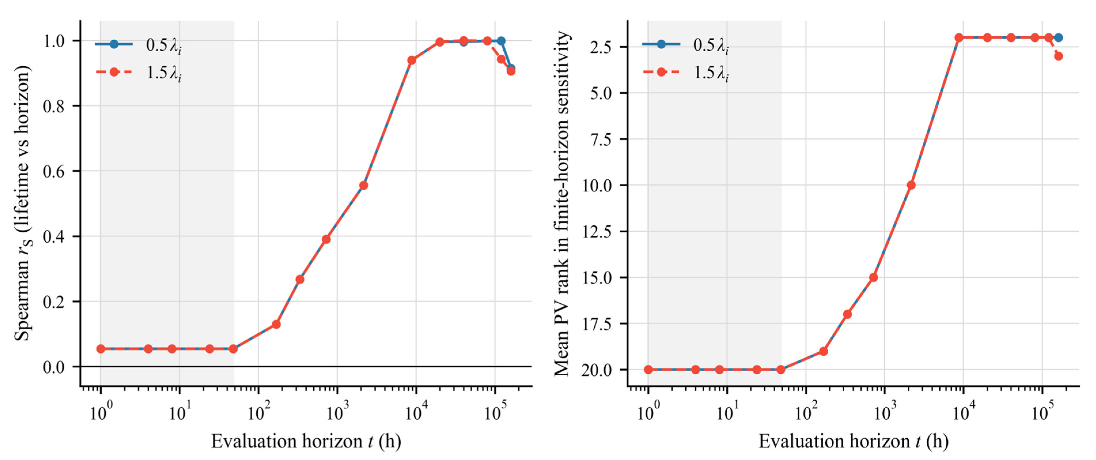
For the independent baseline, the comparison ranks the analytical absolute percentage changes in MTTF and F_s(t) after the same one-at-a-time rate perturbation. For the 0.5λ_i case, one rate is halved, and the other 20 are held fixed. Spearman r_S is calculated as the Pearson correlation of the two average-rank vectors, with tied sensitivities assigned their mean position. The ranks come from unrounded analytical sensitivities in Table 6; the CTF values in Table 4 describe a separate measure. At 24 h, r_S = 0.0546 for factors from 0.1 through 1.5, and 0.485 for the 10-fold stress case. For the 0.5λ_i case, Kendall’s τ_b is 0.149, 0.846, 0.979 and 0.826 at 24, 8,760, 40,000 and 160,000 h, respectively, consistent with the Spearman trend. Tie handling and pair counts are detailed in Supplementary Notes S1 and S3.4. Figure 14 traces the horizon dependence. The shared short-horizon order reflects first-order paths, whose sensitivities scale with perturbation amplitude within this range.

Table 6. Selected analytical OAT sensitivities and average ranks at the 0.5λ_i perturbation.

Events	|ΔMTTF| (%)	Lifetime Rank	|ΔFs(24 h)| (%)	Finite-Horizon Rank
X1–X3 PV modules	20.524 each	2.0	0.000219 each	20.0
X9 protection module	5.874	4.0	0.0439	8.0
X4 battery pack	1.895	5.0	15.367	1.0
X17 satellite link	1.750	6.0	0.0122	9.0
X14–X15 servos	1.256 each	7.5	10.244 each	2.5
X11–X13 computer/sensors	0.468 each	14.0	3.842 each	5.0
X10 brushless motor	0.312	16.0	2.561	7.0
X20–X21 ground computer/return	0.278 each	17.5	0.00359 each	14.5

Figure 14. Tie-aware agreement between lifetime and finite-horizon OAT rankings and the corresponding PV priority. The shaded region denotes the 1–48 h reference range.

All percentage changes in Table 6 are obtained from the analytical solution. For example, the PV value of 0.000219% is a relative change in F_s(24 h), independent of Monte Carlo event counts. Additional digits preserve the ordering of small effects under the specified inputs.

Using 60-digit arithmetic and tie tolerances from 10⁻⁸ to 10⁻⁴⁰ in percentage-point sensitivities gives the same 24 h coefficient. A 200,000-draw label-permutation benchmark preserving tied ranks gives a two-sided p = 0.813 at 24 h. Collapsing the 21 events into 11 symmetry classes gives r_S = 0.264 and p = 0.434; leaving out one event at a time gives −0.010 to 0.221. These are diagnostics for the specified finite event list, conditional on its topology and rates. Supplementary Note S1 documents the randomization rule and full results.

Under independence at short duration, the seven first-order cut sets dominate because their probabilities scale as O(t), whereas the PV path is third order and scales as O(t³). Balancing the leading sensitivity terms for X₁ and X₄ gives a crossover estimate of 6347 h, compared with 7789 h from the exact 0.5-rate solution. The horizon scan resolves this finite-time correction and the dependence of crossings on perturbation amplitude; Supplementary Note S3 gives the derivation.

For the independent baseline, ranking agreement increases with the evaluation horizon: r_S = 0.1297 at 168 h, 0.3904 at 720 h, 0.5563 at 2160 h, 0.9394 at 8760 h and 0.996–1.000 near 40,000 h for the matched 0.5 and 1.5 perturbations. The three PV modules move from a tied mean rank of 20 over 1–48 h to 2 at 8760 h. Accumulation of higher-order failures brings the finite-horizon priorities closer to those obtained by integrating survival over the lifetime. At 160,000 h, the top-event probability is 0.9964; saturation compresses the sensitivities and lowers the correlations to 0.914/0.907. Convergence near 40,000 h identifies a horizon where component-design priorities approximate the lifetime objective; the saturated tail marks the limit of that agreement. Replacement decisions require a maintained-system model.

7. Discussion

The independent-baseline results show a clear dependence of reliability priorities on the evaluation time scale. At the lifetime scale, the three PV modules and the power-protection module X₉ contribute more strongly to system-lifetime sensitivity, whereas the 24 h finite-horizon response is dominated by the battery X₄, the servo subsystems X₁₄–X₁₅, the airborne computer and sensor inputs X₁₁–X₁₃, and the brushless motor X₁₀. This difference follows from the fault-tree structure: first-order cut sets dominate at short durations, while higher-order combinations become increasingly influential over longer horizons. Accordingly, the low tie-aware Spearman correlation at 24 h and its increase with evaluation horizon indicate that lifetime- and finite-horizon analyses reflect different reliability priorities.

The numerical conclusions depend on the functional topology, rate inputs and dependence assumptions. The independent-baseline ranking contrast persists at the sampled 1–48 h points, while longer horizons approach the lifetime ordering. The joint horizon–dependence check shows that PV common causes can elevate short-horizon PV priority and remove the baseline screening margin. Cross-platform implementation checks and rate scans characterize numerical consistency and model response. Transfer to another aircraft requires its functional architecture, operating profile, rate data and dependence mechanisms.

The principal limitations concern dynamics, ageing and functional validation. The static model assumes permanent exponential hardware failures without repair. Detection coverage, reconfiguration, recovery sequences, wear-out and time-varying solar or battery conditions require additional state and stress models [19,20,21,22,23,31]. The battery series criterion and the M₁₅ recovery criterion require validation against bus isolation, control-path substitutability and recovery-success evidence. X₂₁’s trigger share describes first-trigger attribution. The aggregate computer input and cross-subsystem common causes also require configuration-specific assessment. Flight-profile feasibility depends on the energy budget, while software, human factors and external hazards enter the broader operational assessment.

Direct numerical comparison with published UAS studies is affected by differences in top-event definitions, architecture, mission length, and rate data. The MTTF and 24 h probability are therefore interpreted against the analytical and simulation agreement and the declared screening ceilings. At the methodological level, the results complement operational ground-risk models [5,6,7,8,9] and model-based UAS reliability studies [10,11,12,13,14,15,16] by linking a fixed fault-tree structure to time-dependent priority changes. External validation can proceed by supplying the relevant aircraft-specific inputs and comparing predicted event frequencies and ranking crossovers with fleet or test observations.

8. Conclusions

A static fault-tree and Monte Carlo workflow was applied to time-horizon-dependent component importance in a solar-powered field-information-support UAS. With 21 compiled rate inputs, 17 minimal cut sets and independent failures, the analytical MTTF is 43,038.8 h and F_s(24 h) = 9.3701 × 10⁻⁵. PV events dominate lifetime-scale sensitivity, whereas first-order paths dominate at the sampled 1–48 h reference horizons, with r_S = 0.0546 throughout. Ranking agreement increases toward the lifetime scale. PV common-cause scenarios can elevate short-horizon PV priority and exceed the illustrative screening ceiling. The matched-perturbation and horizon-scan workflow supports prioritization conditional on the dependence model and functional topology. Operational use requires validation of the assumed functional-loss criteria and the flight profile.

References

- European Union Aviation Safety Agency, Easy Access Rules for Unmanned Aircraft Systems (Regulations (EU) 2019/947 and (EU) 2019/945), Revision from July 2024. Available online: https://www.easa.europa.eu/en/document-library/easy-access-rules/easy-access-rules-unmanned-aircraft-systems-regulations-eu (accessed on 14 October 2026).
- Joint Authorities for Rulemaking on Unmanned Systems, Specific Operations Risk Assessment (SORA), Main Body, Edition 2.5, JAR-doc-25, 13 May 2024. Available online: https://www.caa.cz/wp-content/uploads/2024/12/SORA-v2.5-Main-Body-Release-JAR_doc_25.pdf (accessed on 14 October 2026).
- SAE International. ARP4761A: Guidelines for Conducting the Safety Assessment Process on Civil Aircraft, Systems, and Equipment; SAE International: Warrendale, PA, USA, 2023. [Google Scholar] [CrossRef] [Scilit]
- SAE International. ARP4754B: Guidelines for Development of Civil Aircraft and Systems; SAE International: Warrendale, PA, USA, 2023. [Google Scholar] [CrossRef] [Scilit]
- Clothier, R.A.; Williams, B.P.; Hayhurst, K.J. Modelling the risks remotely piloted aircraft pose to people on the ground. Saf. Sci. 2018, 101, 33–47. [Google Scholar] [CrossRef] [Scilit]
- Primatesta, S.; Rizzo, A.; La Cour-Harbo, A. Ground risk map for unmanned aircraft in urban environments. J. Intell. Robot. Syst. 2020, 97, 489–509. [Google Scholar] [CrossRef] [Scilit]
- Blom, H.A.P.; Jiang, C.; Grimme, W.B.; Mitici, M.; Cheung, Y.S. Third party risk modelling of UAS operations, with application to parcel delivery service. Reliab. Eng. Syst. Saf. 2021, 214, 107788. [Google Scholar] [CrossRef] [Scilit]
- Oh, S.; Yoon, Y. Data-driven risk analysis of unmanned aircraft system operations considering spatiotemporal population distribution. Transp. Res. Interdiscip. Perspect. 2022, 16, 100732. [Google Scholar] [CrossRef] [Scilit]
- Du, S.; Zhong, G.; Wang, F.; Pang, B.; Zhang, H.; Jiao, Q. Safety Risk Modelling and Assessment of Civil Unmanned Aircraft System Operations: A Comprehensive Review. Drones 2024, 8, 354. [Google Scholar] [CrossRef] [Scilit]
- Petritoli, E.; Leccese, F.; Ciani, L. Reliability and maintenance analysis of unmanned aerial vehicles. Sensors 2018, 18, 3171. [Google Scholar] [CrossRef] [Scilit]
- Tabassum, A.; Sabatini, R.; Gardi, A. Probabilistic Safety Assessment for UAS Separation Assurance and Collision Avoidance Systems. Aerospace 2019, 6, 19. [Google Scholar] [CrossRef] [Scilit]
- Steurer, M.; Morozov, A.; Janschek, K.; Neitzke, K.-P. Model-Based Dependability Assessment of Phased-Mission UAVs. IFAC-Pap. 2020, 53, 8915–8922. [Google Scholar] [CrossRef] [Scilit]
- Liscouët, J.; Pollet, F.; Jézégou, J.; Budinger, M.; Delbecq, S.; Moschetta, J.-M. A methodology to integrate reliability into conceptual design of safety-critical multirotor UAVs. Aerosp. Sci. Technol. 2022, 127, 107681. [Google Scholar] [CrossRef] [Scilit]
- Xiao, Q.; Li, Y.; Luo, F.; Liu, H. Analysis and assessment of risks to public safety from UAVs using FTA and Bayesian network. Technol. Soc. 2023, 73, 102229. [Google Scholar] [CrossRef] [Scilit]
- Wanner, D.; Hashim, H.A.; Srivastava, S.; Steinhauer, A. UAV avionics safety, certification, accidents, redundancy, integrity, and reliability: A comprehensive review and future trends. Drone Syst. Appl. 2024, 12, 1–23. [Google Scholar] [CrossRef] [Scilit]
- Washington, A.; Clothier, R.; Neogi, N.; Silva, J.; Hayhurst, K.; Williams, B. Adoption of a Bayesian belief network for the system safety assessment of remotely piloted aircraft systems. Saf. Sci. 2019, 118, 654–673. [Google Scholar] [CrossRef] [Scilit]
- Vesely, W.E.; Stamatelatos, M.; Dugan, J.B.; Fragola, J.; Minarick, J., III; Railsback, J. Fault Tree Handbook with Aerospace Applications, NASA Office of Safety and Mission Assurance. 2002. Available online: https://extapps.ksc.nasa.gov/reliability/Documents/Fault_Tree_Handbook_with_Aerospace_Applications_August_2002.pdf (accessed on 14 October 2026).
- Dugan, J.B.; Bavuso, S.J.; Boyd, M.A. Dynamic fault-tree models for fault-tolerant computer systems. IEEE Trans. Reliab. 1992, 41, 363–377. [Google Scholar] [CrossRef] [Scilit]
- Bobbio, A.; Portinale, L.; Minichino, M.; Ciancamerla, E. Improving the analysis of dependable systems by mapping fault trees into Bayesian networks. Reliab. Eng. Syst. Saf. 2001, 71, 249–260. [Google Scholar] [CrossRef] [Scilit]
- Boudali, H.; Dugan, J.B. A discrete-time Bayesian network reliability modeling and analysis framework. Reliab. Eng. Syst. Saf. 2005, 87, 337–349. [Google Scholar] [CrossRef] [Scilit]
- Kabir, S.; Walker, M.; Papadopoulos, Y. Dynamic system safety analysis in HiP-HOPS with Petri nets and Bayesian networks. Saf. Sci. 2018, 105, 55–70. [Google Scholar] [CrossRef] [Scilit]
- Zhu, C.; Zhang, T. A review on the realization methods of dynamic fault tree. Qual. Reliab. Eng. Int. 2022, 38, 3233–3251. [Google Scholar] [CrossRef] [Scilit]
- Gradel, S.; Aigner, B.; Stumpf, E. Model-based safety assessment for conceptual aircraft systems design. CEAS Aeronaut. J. 2022, 13, 281–294. [Google Scholar] [CrossRef] [Scilit]
- Birnbaum, Z.W. On the importance of different components in a multicomponent system. In Multivariate Analysis, II; Academic Press: Cambridge, MA, USA, 1969; pp. 581–592. [Google Scholar]
- Cheok, M.C.; Parry, G.W.; Sherry, R.R. Use of importance measures in risk-informed regulatory applications. Reliab. Eng. Syst. Saf. 1998, 60, 213–226. [Google Scholar] [CrossRef] [Scilit]
- Xu, A.; Zhang, Z.; Zhang, H.; Wang, H.; Zhang, M.; Chen, S.; Ma, Y.; Dong, X. Research on Time-Dependent Component Importance Measures Considering State Duration and Common Cause Failure. Front. Energy Res. 2020, 8, 584750. [Google Scholar] [CrossRef] [Scilit]
- Borgonovo, E.; Plischke, E. Sensitivity analysis: A review of recent advances. Eur. J. Oper. Res. 2016, 248, 869–887. [Google Scholar] [CrossRef] [Scilit]
- IEC 61709:2017; Electric Components—Reliability—Reference Conditions for Failure Rates and Stress Models for Conversion. International Electrotechnical Commission: Geneva, Switzerland, 2017. Available online: https://webstore.iec.ch/en/publication/28554 (accessed on 14 October 2026).
- SAE International. ARP5890B: Guidelines for Preparing Reliability Assessment Plans for Electronic Engine Controls; SAE International: Warrendale, PA, USA, 2018. [Google Scholar] [CrossRef] [Scilit]
- U.S. Department of Defense. MIL-HDBK-217F Notice 2: Reliability Prediction of Electronic Equipment. 1995. Available online: https://quicksearch.dla.mil/qsDocDetails.aspx?ident_number=53939 (accessed on 30 September 2026).
- Aghaei, M.; Fairbrother, A.; Gok, A.; Ahmad, S.; Kazim, S.; Lobato, K.; Oreski, G.; Reinders, A.H.; Schmitz, J.; Theelen, M.; et al. Review of degradation and failure phenomena in photovoltaic modules. Renew. Sustain. Energy Rev. 2022, 159, 112160. [Google Scholar] [CrossRef] [Scilit]
- Hughes, R.P. A new approach to common cause failure. Reliab. Eng. 1987, 17, 211–236. [Google Scholar] [CrossRef] [Scilit]
- Hokstad, P. A shock model for common-cause failures. Reliab. Eng. Syst. Saf. 1988, 23, 127–145. [Google Scholar] [CrossRef] [Scilit]
- Quanterion Solutions Incorporated, Nonelectronic Parts Reliability Data (NPRD-2023), Utica, NY, USA. 2023. Available online: https://www.quanterion.com/product/publications/nprd-2023-hard-copy/ (accessed on 30 September 2026).
- Quanterion Solutions Incorporated, Electronic Parts Reliability Data (EPRD-2024), Utica, NY, USA. 2024. Available online: https://www.quanterion.com/product/publications/eprd-2024-hard-copy/ (accessed on 30 September 2026).
Disclaimer/Publisher’s Note: The statements, opinions and data contained in all publications are solely those of the individual author(s) and contributor(s) and not of MDPI and/or the editor(s). MDPI and/or the editor(s) disclaim responsibility for any injury to people or property resulting from any ideas, methods, instructions or products referred to in the content. |
© 2026 by the authors. Licensee MDPI, Basel, Switzerland. This article is an open access article distributed under the terms and conditions of the Creative Commons Attribution (CC BY) license.