


Abstract
In time-marching simulation of airborne wind energy systems (AWESs), the tether is usually discretised into a series of lumped masses (i.e., nodes) connected by spring and damper elements. There is no consensus on the appropriate number of nodes for AWES applications, although it is known that using more nodes than necessary is computationally costly. In this work, we examine the trim solutions of a fixed-wing aircraft connected to the ground by a 500 m tether. A successive difference metric is proposed to quantify the convergence rate of the trim solutions as more nodes are added. We then compare this gain in accuracy to the simulation time and memory usage by plotting their Pareto fronts. Results reveal that using 6–8 tether nodes (i.e., 7–9 segments) is sufficient. Compared to using 15 nodes, 8 nodes keep the successive difference metric below 2%, run over 13 times faster, and require less than a quarter of memories. Beyond 8 nodes, the differential equation solver appears to enter a new stiffness regime, resulting in rapid rises in computation time and memory usage. These findings suggest that the conservative choices of 10–20 nodes can be relaxed, promising significantly lower computation costs in future studies.
1. Introduction
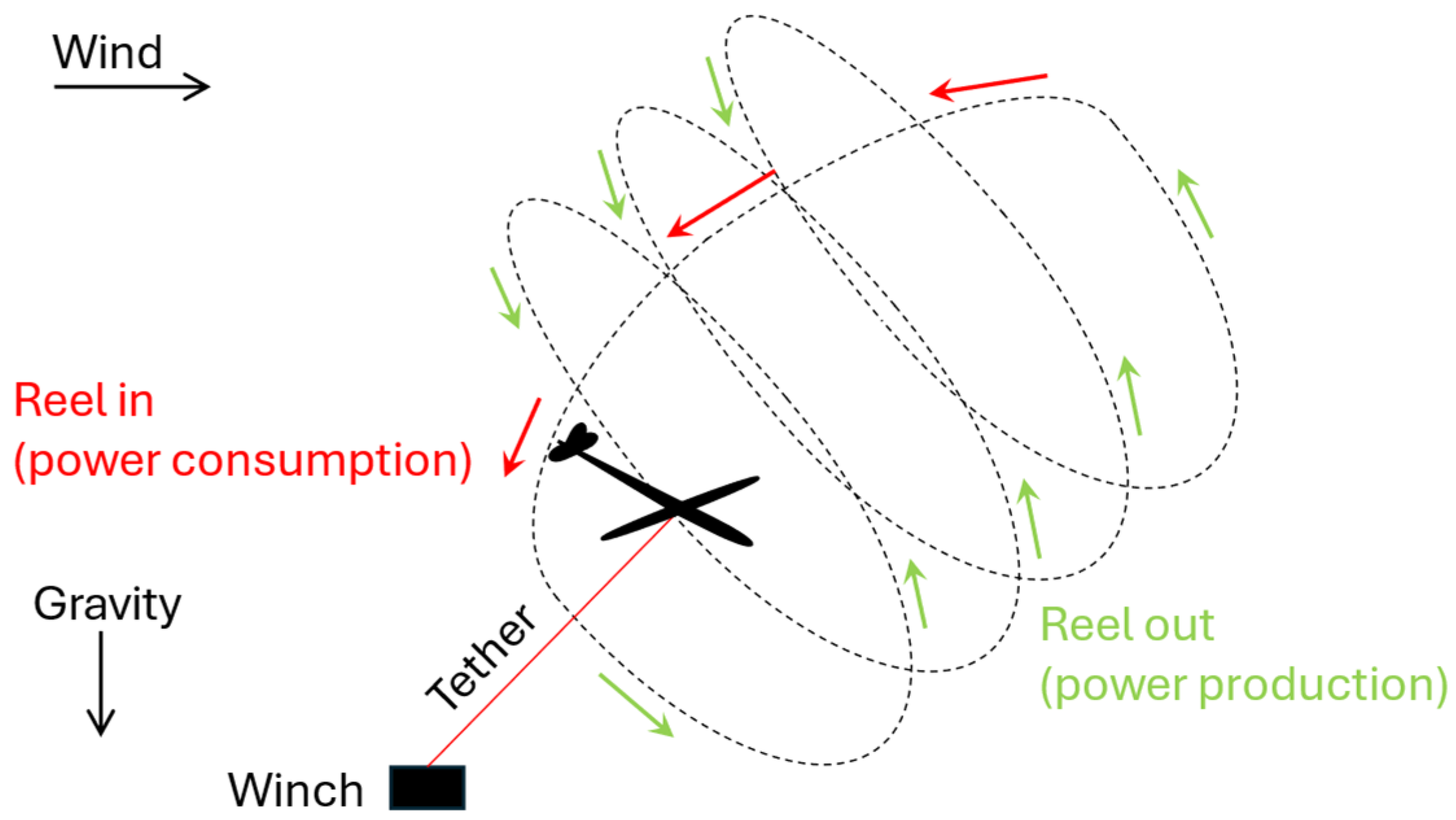
Airborne wind energy systems (AWESs) are an emerging technology for electricity generation using tethered flying devices. AWES provide several advantages over conventional wind turbines, most notably the ability to relocate, lower lifecycle material usage, and a higher capacity factor. In the groundgen configuration, the flying device (commonly referred to as a kite in the literature) performs wind-powered flights to pull a cable (tether) connected to a ground-based station. The mechanical power delivered by the tether tension is transformed into electrical power at the generator. Figure 1 illustrates the operating principle of a typical groundgen system. The winch, which forms part of the ground station, is responsible for controlling the rate at which the tether is reeled in or out. For an overview of AWES technology and its progression over the past decade, including other configurations beyond groundgen, readers can refer to three systematic reviews published between 2015 and 2025 [1,2,3]. Also worth mentioning are two books that summarise key technical concepts [4,5].
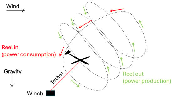
Figure 1.
Schematic of a full pumping cycle in a groundgen AWES, comprising a reel-out phase (shown here in circular-pattern flight) followed by reel-in.
From a flight dynamics perspective, AWES are characterised by the presence of the tether, which partially constrains the dynamics and adds considerable drag. An overview of different tether modelling methods can be found in Section 2 of [6]. In most AWES studies, the tether is usually modelled as either a rigid rod or a series of straight and elastic segments, each bounded by a pair of lumped masses connected by spring and damper elements. The rigid rod approach is common among both early studies and a few advanced simulation-based analyses due to its simplicity. Simulation results can be considered accurate if the tether tension remains high, thereby minimising tether bending, and the variation in aerodynamic force along the tether length is negligible. In practice, AWES can operate at altitudes exceeding 500 m, resulting in varying wind speed, local flow angle, and air density along the tether length and hence different aerodynamic forces. The straight-line assumption is no longer valid in such cases, thereby requiring a multi-segment modelling method. In this instance, users must decide on the discretisation level, i.e., the number of lumped mass elements (i.e., nodes) used to model the tether. There is currently no general guideline on the appropriate number of nodes for AWES applications. A non-exhaustive survey on the number of tether nodes used in academic studies is provided in Table 1, where ‘0 node’ refers to the rigid rod approach. Note that the discretisation level can be described by either the number of tether nodes (also referred to as ‘particles’) between the ground winch and the kite or the number of tether segments (or ‘sections’), which equals the number of nodes plus one. Both terminologies are common in the literature. In this work, we describe the discretisation level by the number of nodes. Table 1 contains a few duplicate entries, which are studies that consider different tether configurations (e.g., designing a controller on a rigid tether, then verifying the controller on a multi-node tether like in [7], or multi-aerofoil AWES concepts with multiple tethers of different lengths [8]). Some well-known studies are not included, as they only mention the use of multi-node modelling without specifying the exact number of nodes used. Similarly, the number of zero-node studies is much higher than those included here, as the majority of early AWES studies rely on the rigid-tether assumption.
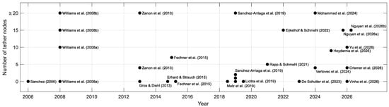
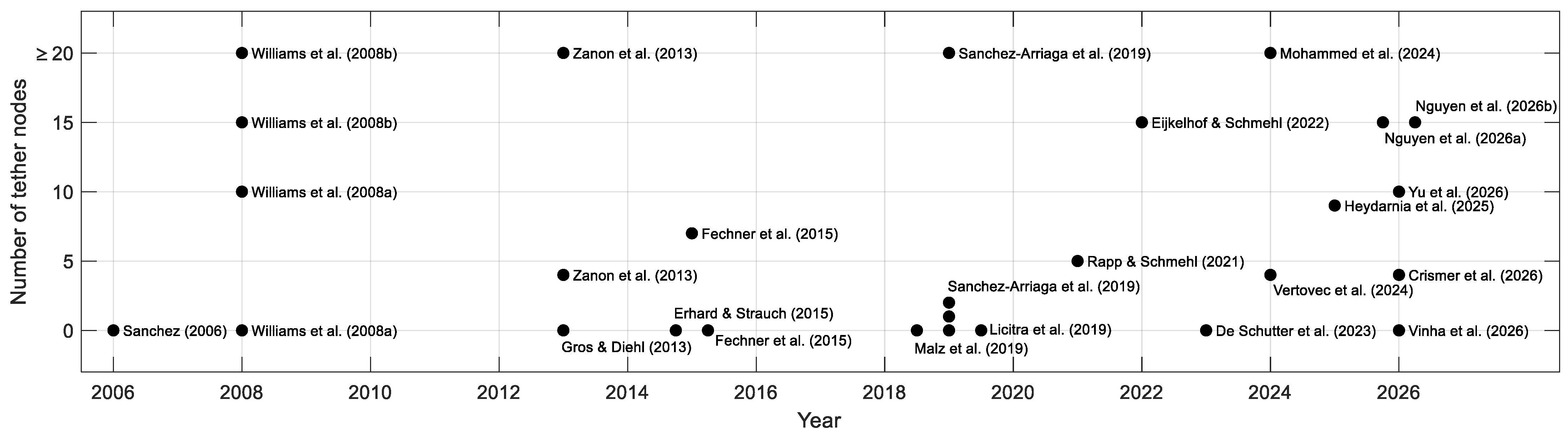
The studies listed in Table 1 are plotted against the time axis as shown in Figure 2, revealing that there is no trend in the number of nodes used. Across the span of 20 years, the zero-node approach remains dominant, while multi-node studies cover a large range from four to over 20 nodes. This lack of convergence outlines the need for a ‘rule of thumb’ for tether discretisation, as an overly conservative approach of using more nodes than necessary incurs heavy computation cost. The closest study to achieve this was done by Sánchez–Arriaga et al. in 2019 [9], which investigates the computation cost of using more nodes. This study highlighted the differences in simulated responses between zero and multiple nodes and noted that going beyond three segments (i.e., two nodes) did not change the response significantly. Whilst the differences mentioned in [9] were not formally quantified beyond an ‘eye test’, they provide one of the first remarks on the advantage of using fewer nodes.
Figure 2.
Tether node count in academic studies between 2006 and 2026 [7,8,9,10,11,12,13,14,15,16,17,18,19,20,21,22,23,24,25,26,27].
Table 1.
Brief survey of tether node count.
This work is motivated by the need to quantify the appropriate number of tether nodes for AWES simulation. Rather than relying on visual inspection of converging trends, we propose a successive difference metric that examines the changes in trim solutions across a range of tether node counts at different operating points. This trim analysis is then combined with time-marching simulations, which determine the accuracy improvement for each additional tether node and weigh it against the associated increase in solver runtime and memory usage. This approach identifies the point beyond which further discretisation is no longer justified by the additional computation cost incurred.
In subsequent sections, the numerical simulation used is described in Section 2. Trim analysis is done in Section 3, which generates a set of data to be analysed by the successive difference metric presented in Section 4.1. This analysis is followed by a comparison against computation costs in Section 4.2. Lastly, Section 5 provides concluding remarks.
2. Simulation Environment
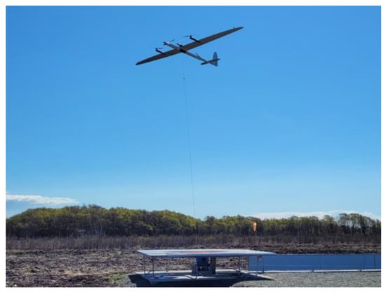
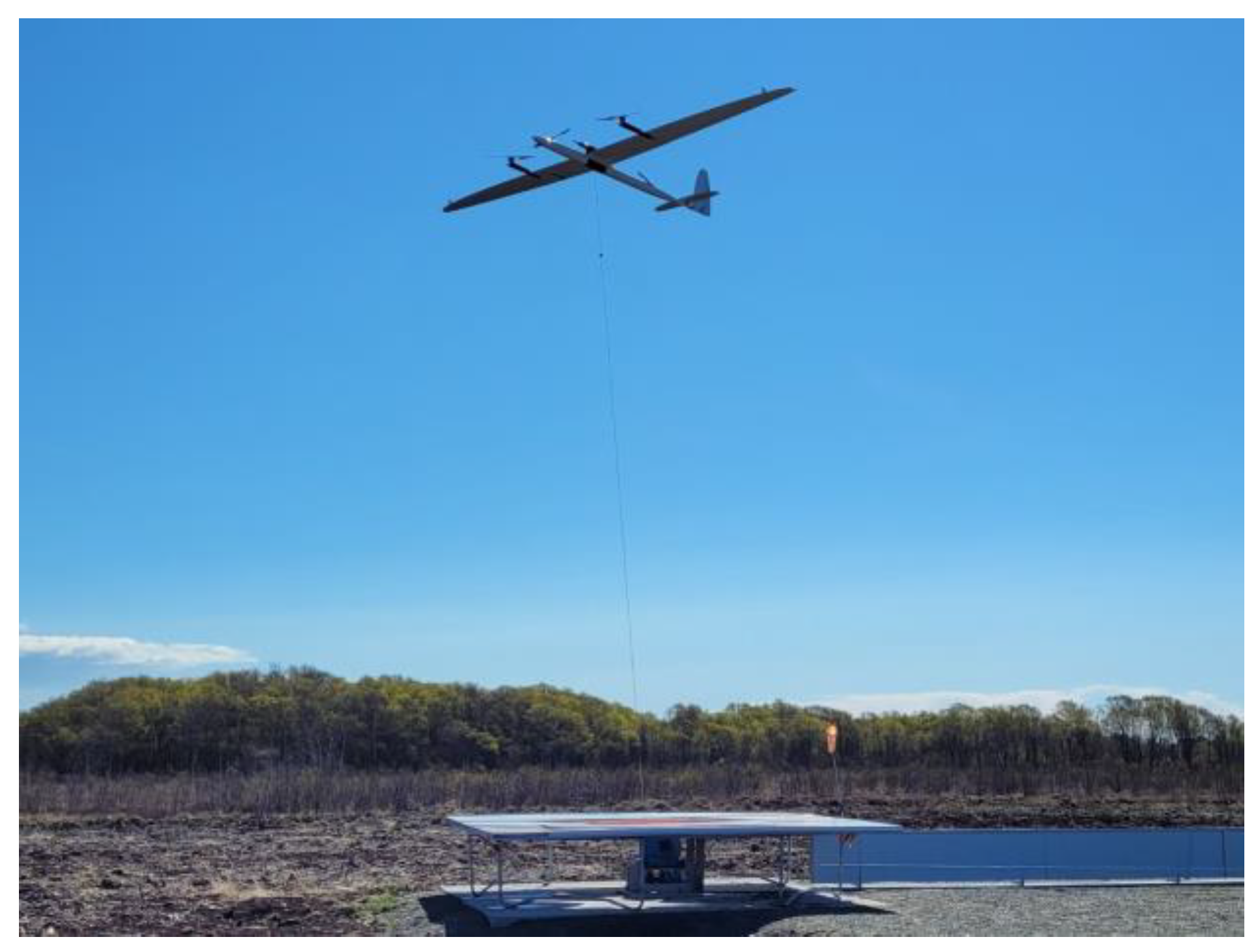
This study uses a six-degree-of-freedom simulator of Kitemill’s KM1 prototype—a 20 kW groundgen system driven by a rigid-wing unmanned aerial vehicle, shown in Figure 3. The aerial vehicle weighs 57 kg and features a high aspect ratio wing, measuring 7.42 m in wingspan and 0.431 m in mean aerodynamic chord. Traditional trailing-edge control surfaces (aileron, elevator, and rudder) are used for flight control, in addition to flaps for increased lift during power production. Aerodynamic data of the KM1 airframe were obtained from computational fluid dynamics and saved as nonlinear polynomials, which are provided in Section 1 of [28].
Figure 3.
Kitemill’s KM1 fixed-wing groundgen AWES prototype.
The simulator was constructed in MATLAB. In its open-loop configuration, 12 states are used to describe the aircraft’s motion in 3D space and 6N states to model the flexible tether, where N is the number of tether nodes between the winch and the aircraft. The N nodes discretise the tether into N + 1 segments. Gravitational, aerodynamic, and elastic forces are calculated for each segment and then distributed equally to the two adjacent nodes. Each node’s acceleration can then be calculated using Newton’s second law. The ground winch is not used in this study, thereby fixing the tether’s natural length at 500 m. A detailed description of the simulator’s equations of motion can be found in [29]. Table 2 lists the tether parameters, and Table 3 summarises the states, control surface inputs, and a few outputs of interest for this paper. Further details on the tether model are provided in Appendix A.
Table 2.
Tether parameters.
Table 3.
Key elements of the simulator.
3. Trim Analysis
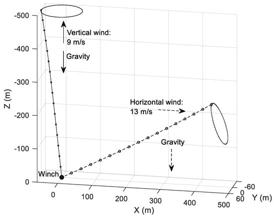
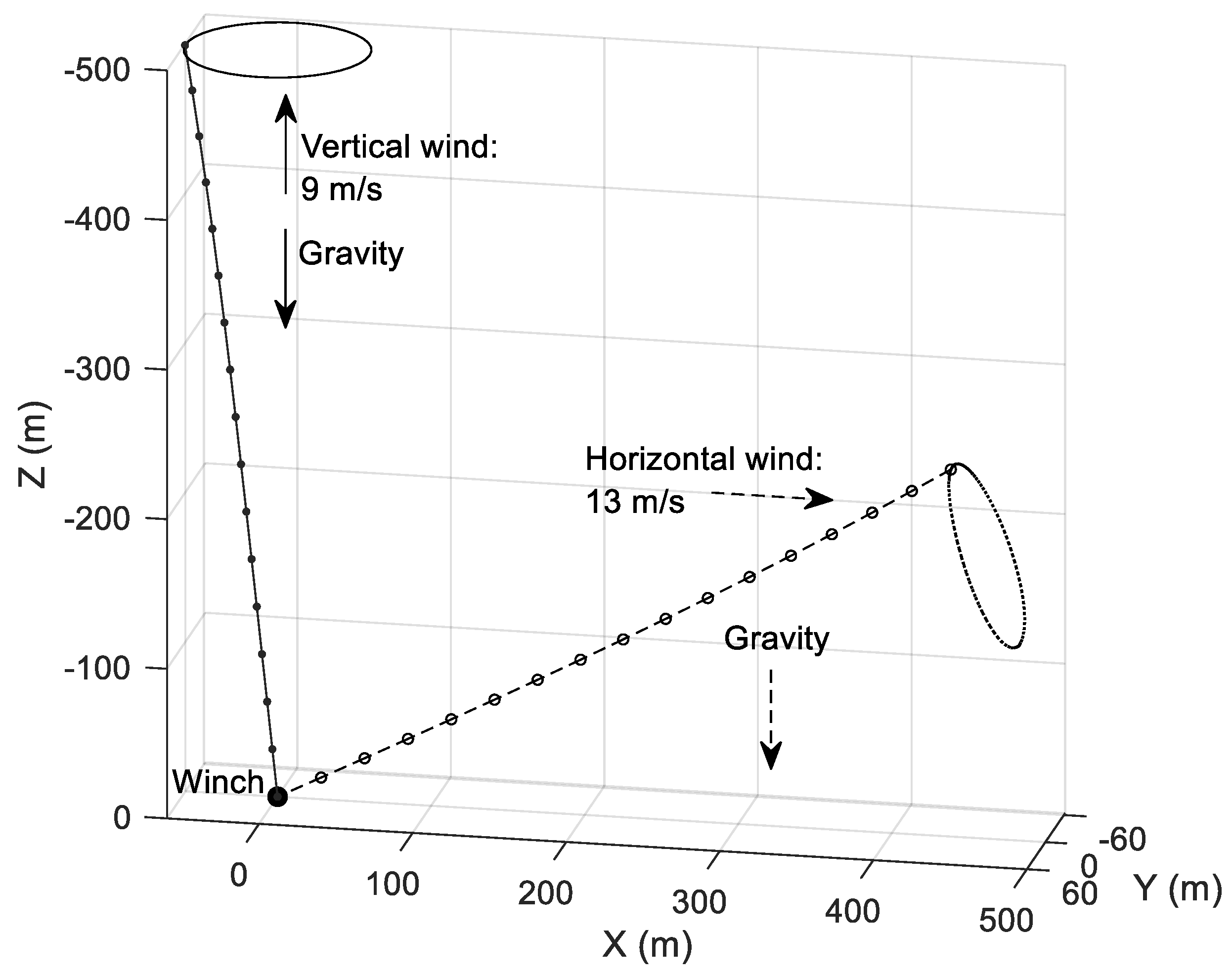
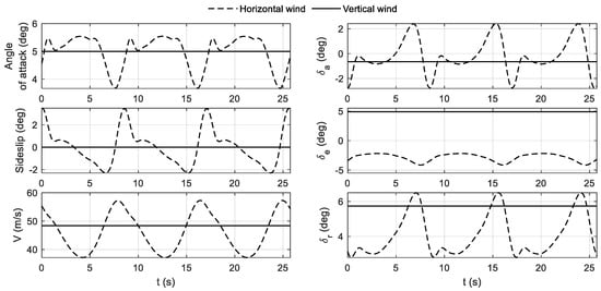
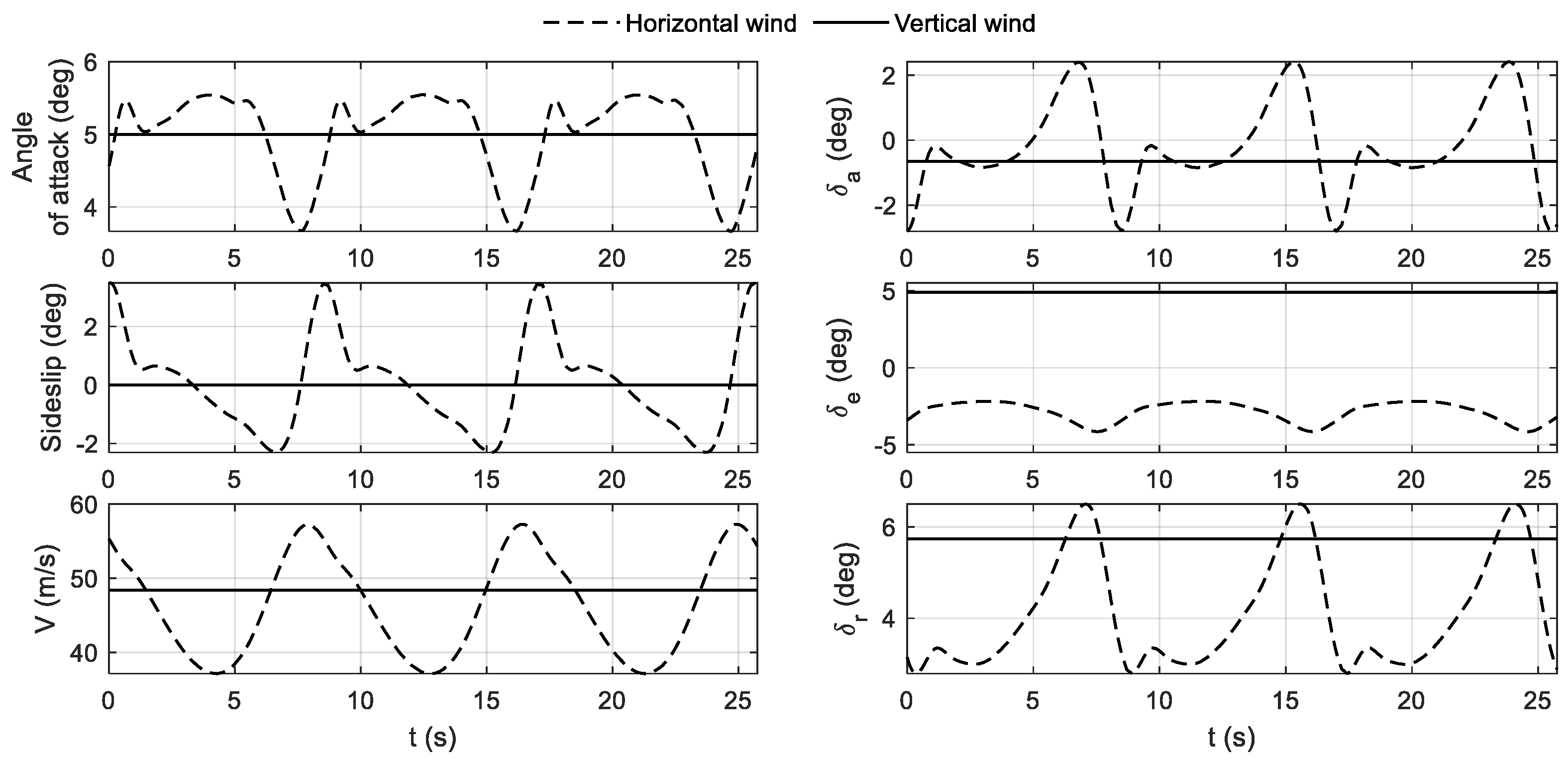
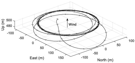
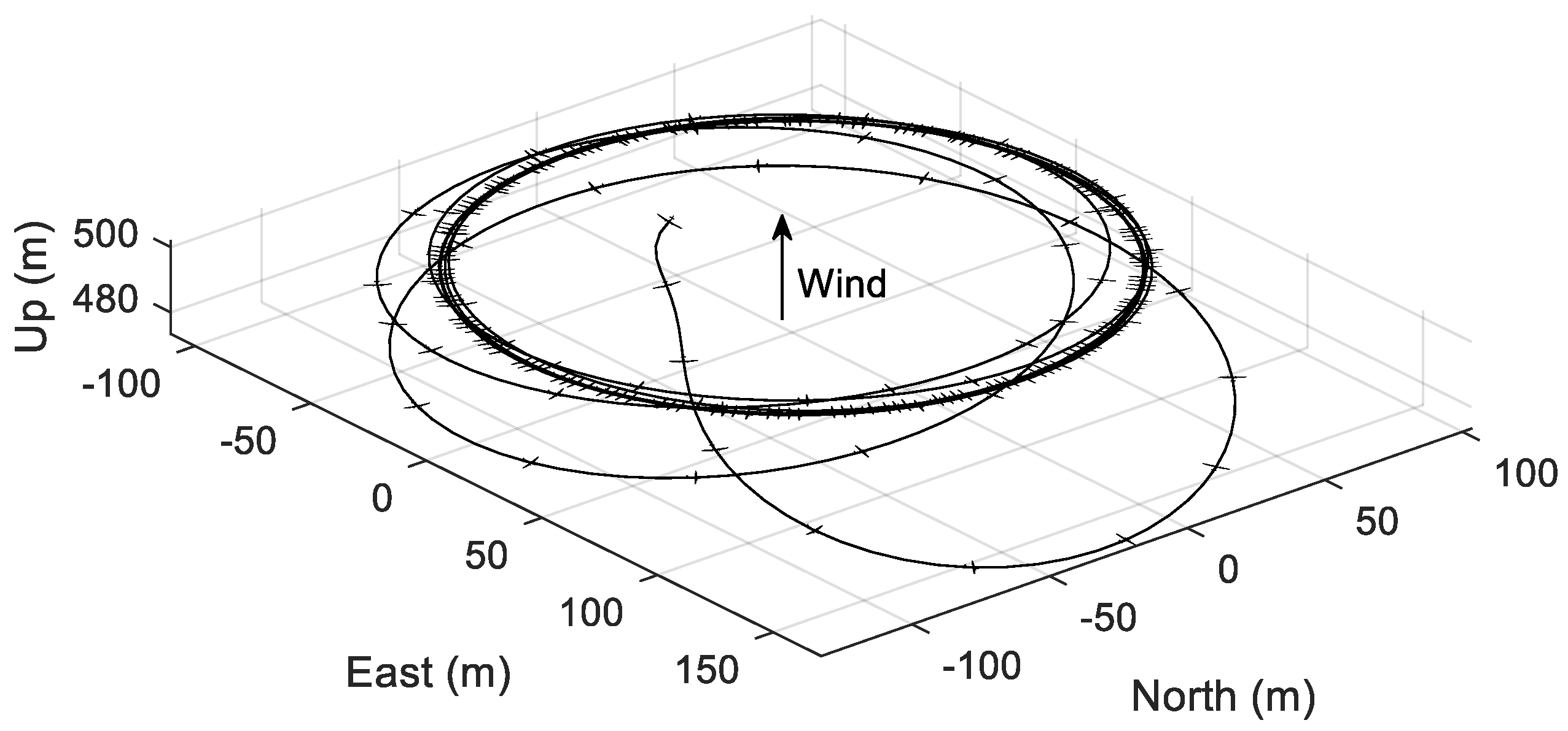
During circular reel-out, gravity acts as an external periodic disturbance that destroys equilibria [25,30]. The issue is illustrated in Figure 4. Consider the circular trajectory depicted by the dashed lines, which has a radius of 60 m and is flown in a uniform horizontal wind field of strength 13 m/s. Since the circle is not normal to the wind direction or gravity, out-of-plane wind and gravitational force become two periodic disturbances that change direction relative to the kite’s body at different points on the circle. It has been shown that cyclic control inputs are required to maintain circular flights in these instances [25,30], and the resulting trajectory is a limit cycle. In the example in Figure 4, we use the flight controller in [31] to track 5° angle of attack and 0° sideslip while keeping the kite in orbit with a 60 m radius. The resulting closed-loop response is shown in Figure 5, where the periodic nature of the dynamics can be seen.
Figure 4.
Circular flight trajectory with vertical wind and horizontal wind. Both cases use a fixed tether length of 500 m discretised into 15 nodes.
Figure 5.
Trimmed flight at 5° angle of attack and zero sideslip. The response to horizontal wind spans three cycles.
Since trim analysis favours equilibrium solutions, the periodic disturbances must be removed. One method to do so is to ignore gravity and bring the circle’s centre down to a height of zero (so that the circle is perpendicular to the wind) [25]. This approach is avoided here, as the effect of gravity on the tether shape and hence aerodynamic drag is significant. Instead, we consider a hypothetical scenario with vertical wind, where the orbit plane is parallel to the ground (see Figure 4). This arrangement was chosen to retain the existence of equilibrium solutions while still reflecting gravity’s contribution to the aircraft and tether dynamics, thereby keeping the results relevant to AWES applications. The vertical wind speed is fixed at 9 m/s throughout this study (except for in Figure 12). This wind speed was chosen to achieve a similar airspeed and hence performance to the 13 m/s horizontal wind case in Figure 4 and Figure 5. Trim solutions are calculated using the Dynamical Systems Toolbox [32], which is the MATLAB implementation of the numerical continuation software AUTO AUTO-07P [33].
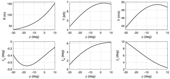
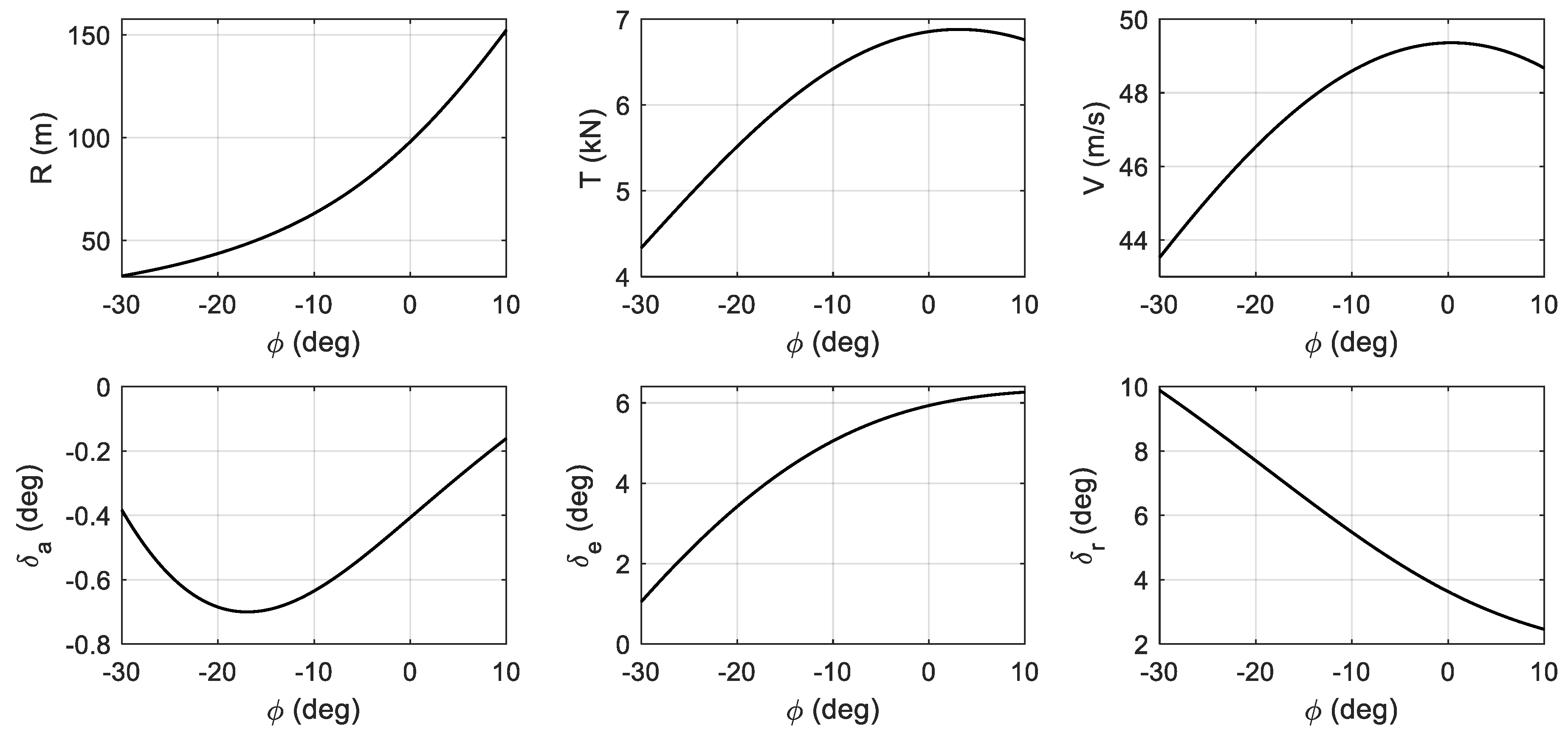
With the pitch and yaw control surfaces allocated to maintain the angle of attack and sideslip, rolling becomes the only mechanism to change the circle radius. Assuming the circle centre is on the left (port) wing, a more negative roll angle ϕ results in a tighter circle. Figure 6 shows the relationship between roll angle and six parameters of interest when 15 tether nodes are used. Apart from the three control surface deflections, which are directly related to trim analysis, the other three parameters (radius R, tether tension T, and airspeed V) are chosen for their relevance to the power generation and flight performance of airborne wind energy systems. The observed trend in each of the six parameters is typical. Key features include the radius diagram having a positive slope and the tether tension reaching its maximum value when the kite rolls slightly away from the turn [25].
Figure 6.
Trim diagram with 15 tether nodes.
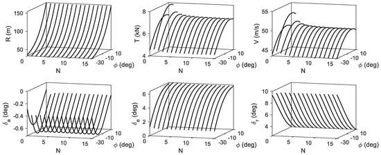
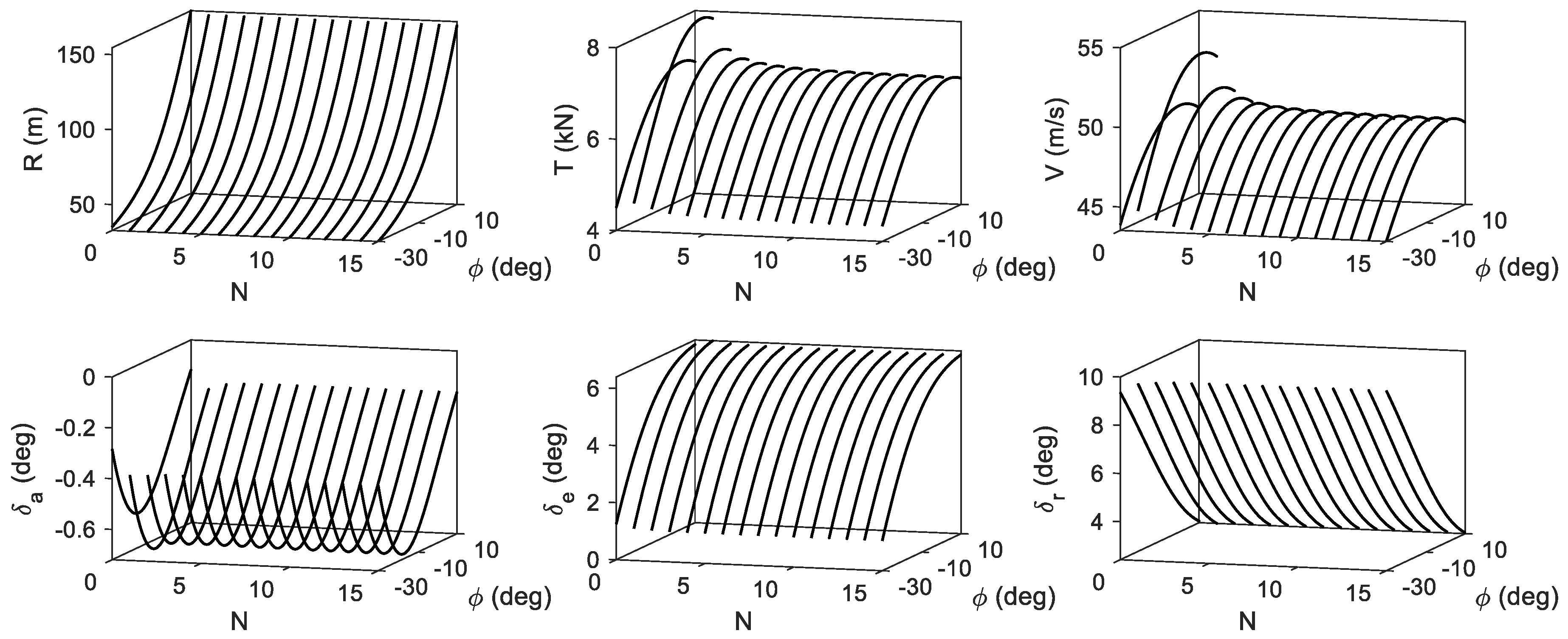
The same trim analysis is done for a range of tether nodes from zero to 15 in increments of one, resulting in six surface plots shown in Figure 7. For convenience, we discretise the data in Figure 7 into a uniform grid with two independent variables: ϕ ∈ [−30°, 10°] in 1° increments, and N ∈ [0, 15] in increments of one. It can be seen that as the number of nodes increases, the trim solutions converge to an apparent ‘ground truth’ value. Also worth noting is that the one-node case deviates the most from other instances. This set of trim data in Figure 7 is used in the following section to determine an appropriate number of tether nodes that balances both accuracy and computational performance.
Figure 7.
Trim diagrams for a range of tether nodes.
4. Results and Discussions
4.1. Convergence Analysis
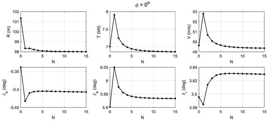
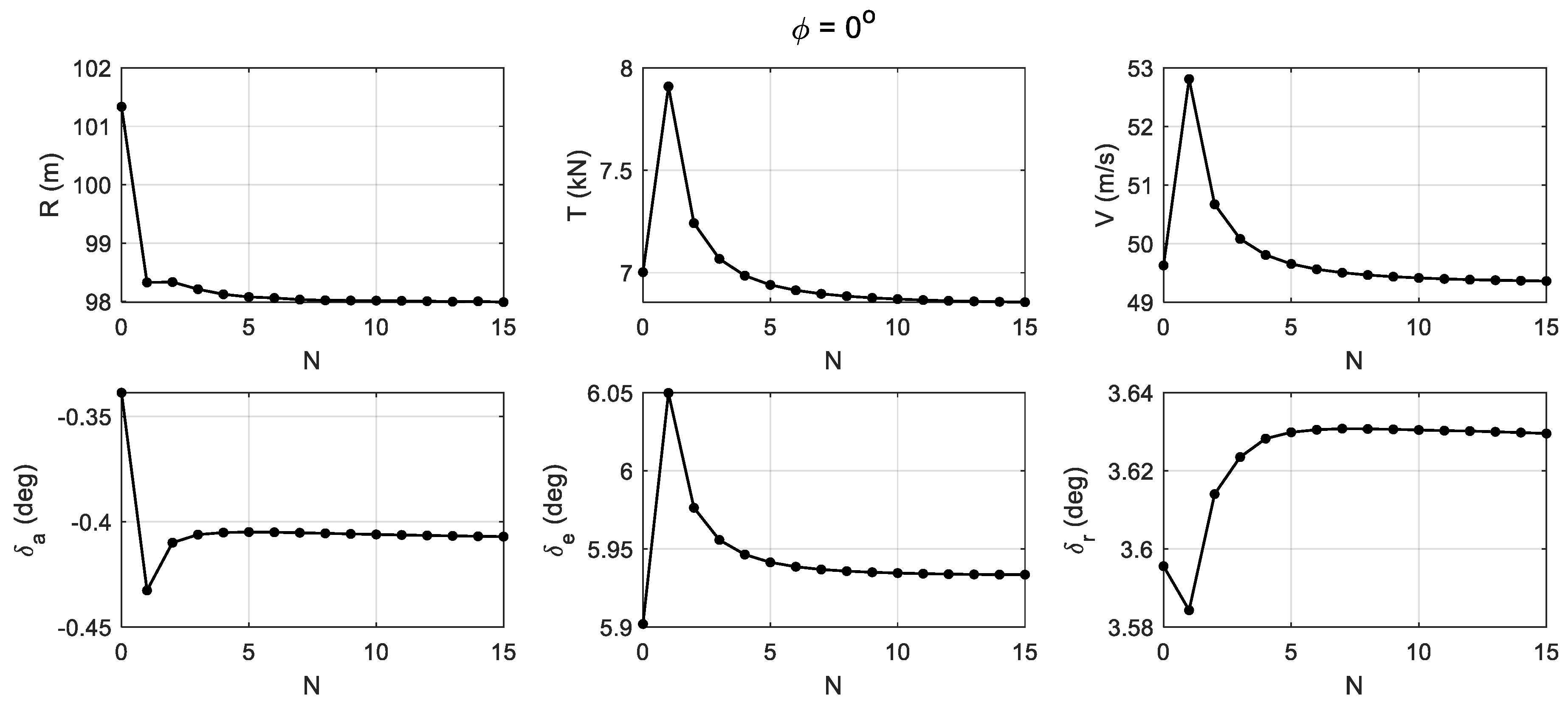
Consider a slice of the trim surface obtained at ϕ = 0°, as shown in Figure 8. As expected, adding more tether nodes results in the trim solutions converging to an apparent final value. In terms of successive differences in the trim solution (i.e., the slope approaching zero as N increases), an ‘eye test’ suggests that no more than 10 nodes are needed, as the slope appears to have levelled out by that point.
Figure 8.
Trim diagram at wing-level flight, showing the impact of adding tether nodes.
To accurately quantify the number of nodes needed, it is necessary to use a convergence criterion that accounts for the slope change in the trim data. We propose a successive difference measurement σ, which was derived based on discussions with the large language model Claude Sonnet 4.6. The method to calculate σ is presented below:
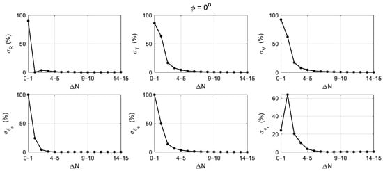
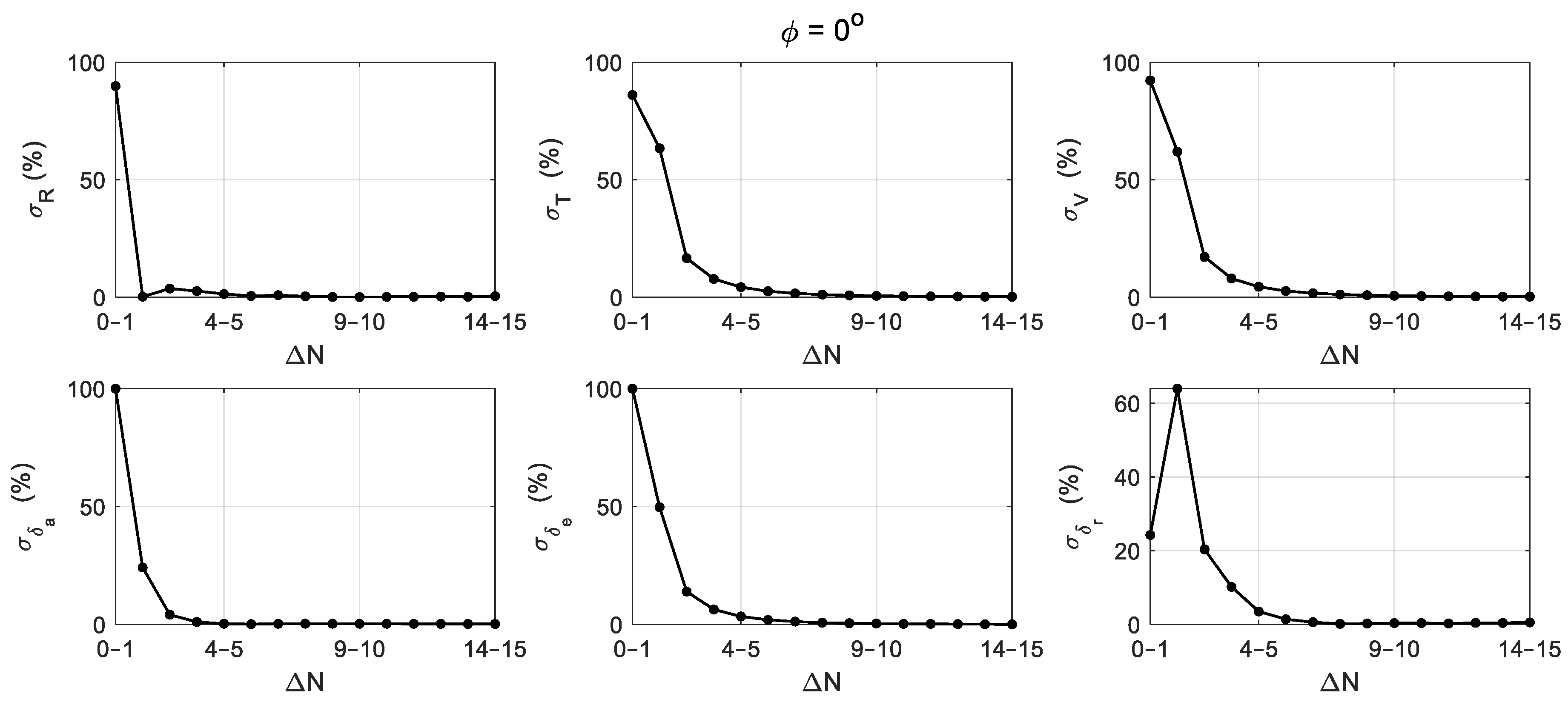
Using Figure 8 as an example, in each of the six plots, calculate the difference between each data point as N increases, then divide this number by the data range (i.e., the difference between the largest and smallest values in each of the six plots). Completing this step results in six plots for σ as shown in Figure 9. In essence, Figure 9 shows how much the trim solution changes relative to the data range as more tether nodes are added. As N increases, σ approaches zero, which indicates that each additional tether node results in smaller changes to the trim solutions.
Figure 9.
Accuracy metric σ for each of the six parameters considered with ϕ fixed at 0°.
Repeat the procedure for the full range of roll angles considered (in this study: ϕ ∈[−30°, 10°] in 1° increments). Doing so results in 41 lines for each of the six parameters considered.
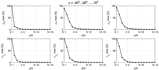
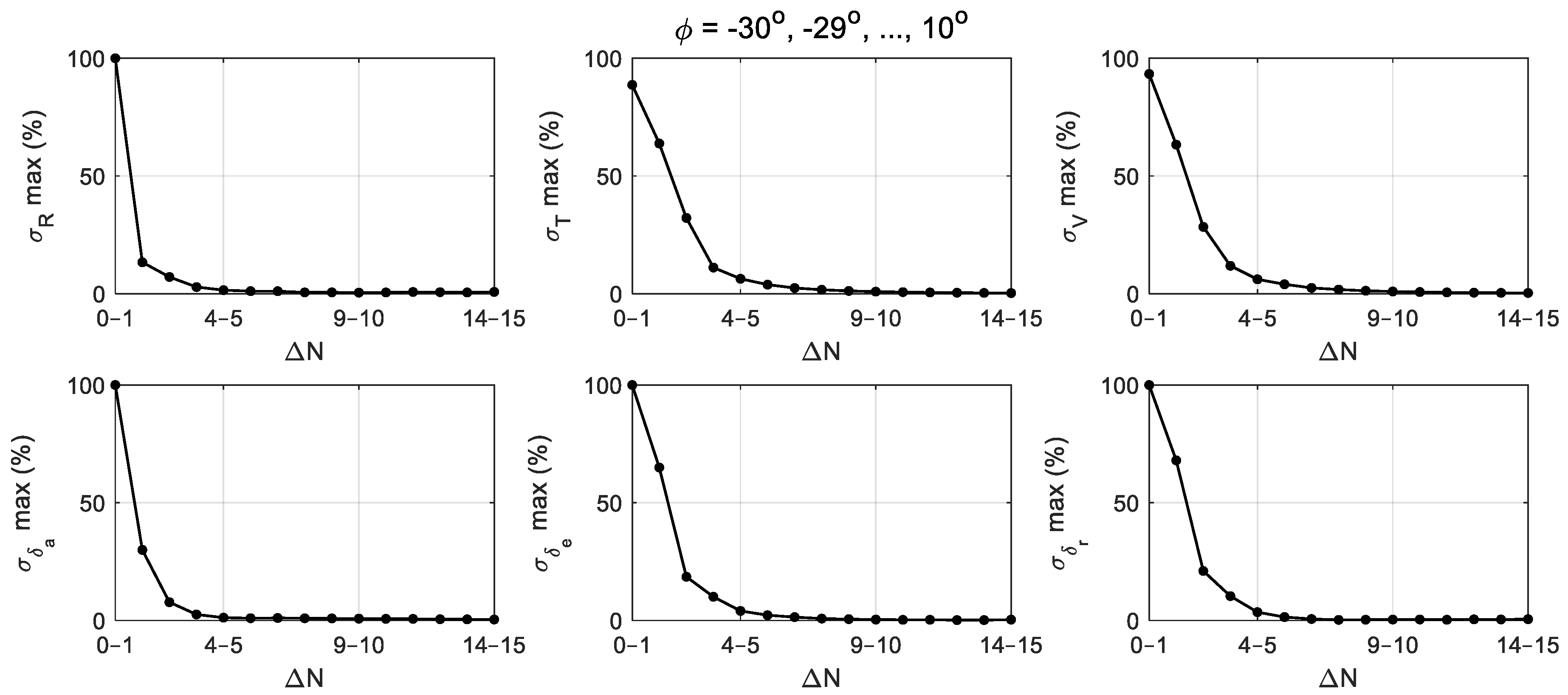
For each value of ΔN, pick the highest σ among the 41 possible choices, then plot those values against ΔN as shown in Figure 10. This step identifies the largest normalised changes in trim solutions across all roll angles as we add more tether nodes.
Figure 10.
Worst-case σ values across the range of roll angles considered.
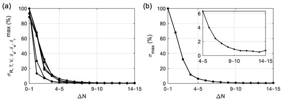
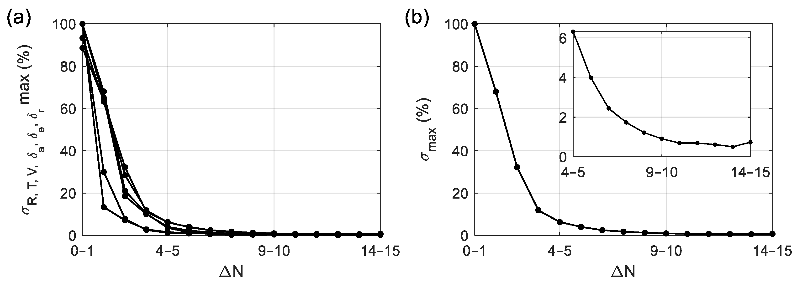
Lastly, plot the six lines in Figure 10 on the same diagram (see Figure 11a), then pick the highest point for each value of ΔN. Completing this step produces Figure 11b, which shows the largest normalised change in trim solution across a seven-dimensional space: roll angle and the six parameters considered.
Figure 11.
(a) Maximum σ for each of the six parameters across the roll angles considered and (b) combined worst-case σ metric. The inset in (b) shows a magnified view.
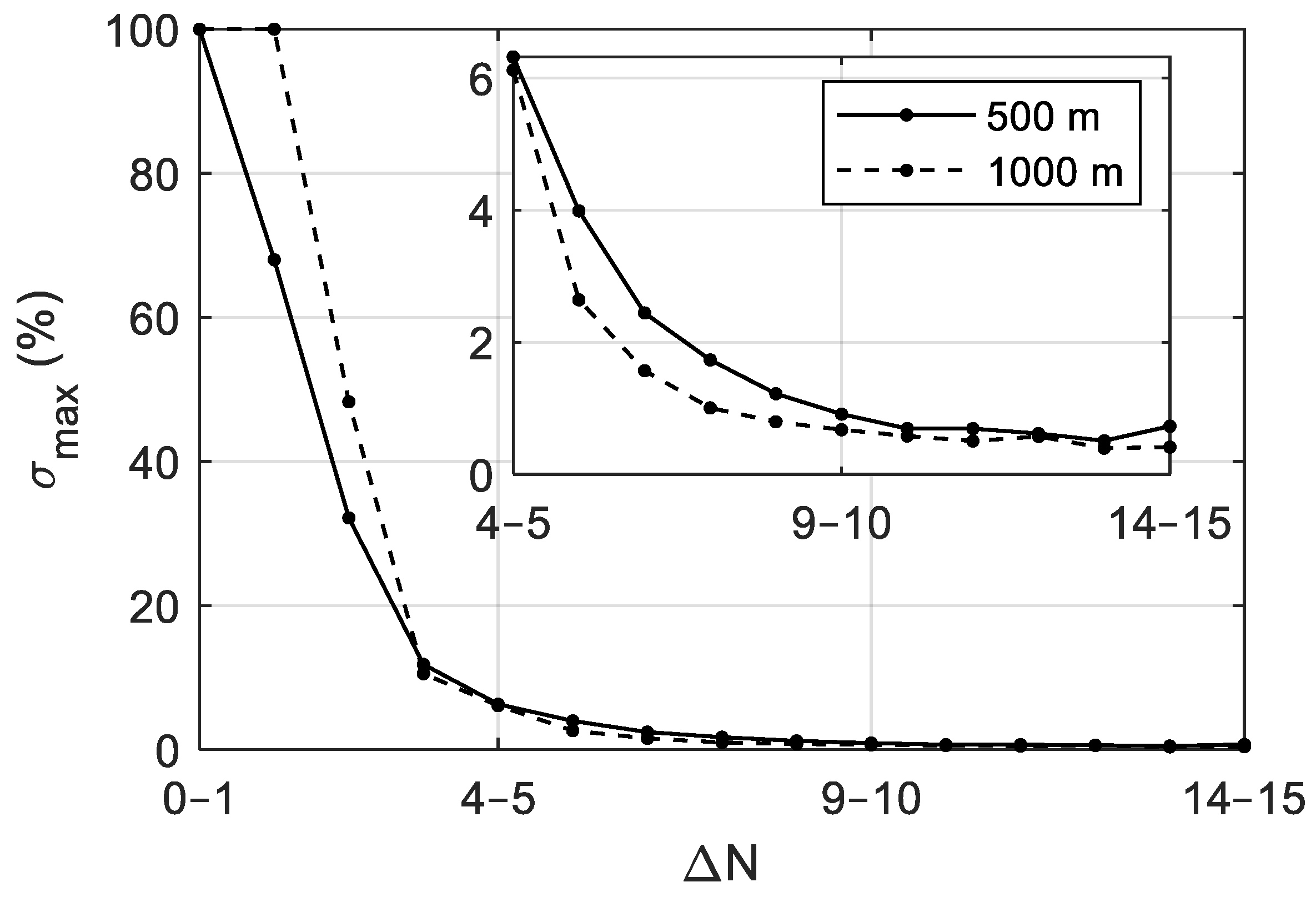
Figure 11b enables users to determine the gain in accuracy (or more accurately, a reduction in relative error) obtained by adding one tether node. From here, the number of nodes required can be found by setting a cutoff point for the successive difference metric. If σmax must remain below 5%, for instance, then six nodes are sufficient. Increasing to 10 nodes reduces σmax to less than 1%.
For additional verification, the analysis is repeated with the tether length doubled from 500 m to 1000 m. Figure 12 shows σmax for both the old and new tether lengths. Interestingly, the two lines cross each other as the number of nodes increases from three to four, indicating that the minimum number of nodes needed is higher for a longer tether. The recommended node count is similar for both cases: six nodes are still sufficient to remain below the 5% threshold, and nine nodes now bring σmax to below 1%. As the 500 m case is slightly more unforgiving, it will be used for the rest of the paper.
Figure 12.
Combined σ metric with two different tether lengths.
4.2. Computation Costs
Using more nodes creates a stiffer system with more tether states, which requires smaller solver steps. The consequences are significantly higher computation time and memory usage, which should be quantified against any improvement in accuracy. To examine the computation cost, we examine a closed-loop step response in the demanded roll angle from −25° to 0° with the initial condition for the simulator set to trimmed flight at ϕ = −25°. The simulation time is set to 200 s. Figure 13 shows the closed-loop response when 15 tether nodes are used. This manoeuvre was chosen because it contains both transient responses (which usually allow larger solver steps) and the subsequent convergence to steady-state trim (requiring smaller steps).
Figure 13.
Step response in demanded roll angle, showing the trajectory with 15 tether nodes. The kite is drawn to scale at 1 s intervals.
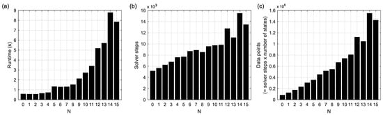
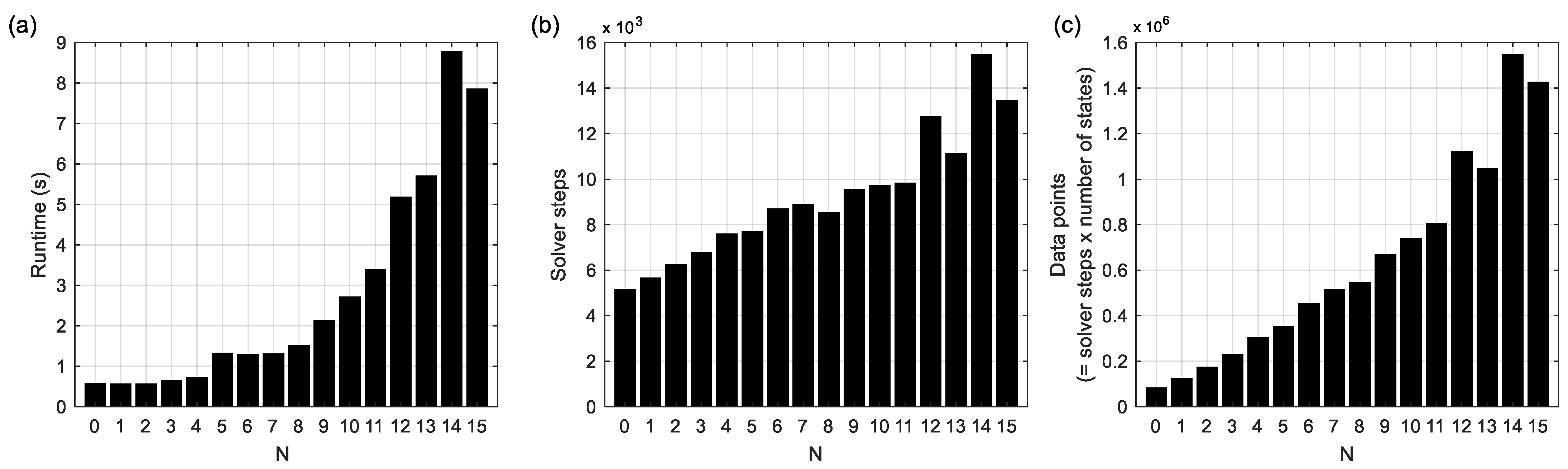
Figure 14 presents the computation cost, which was generated using MATLAB’s ordinary differential equation (ODE) solver ode23t using a relative tolerance of 1 × 10⁻² and absolute tolerance of 1 × 10⁻⁵—both are one order of magnitude lower than MATLAB’s default values. Further performance enhancement was achieved by compiling the simulator into a C-code MEX file. Results in Figure 14 suggest an exponential increase in runtime and a linear increase in both solver steps and memory usage. Furthermore, the runtime values appear to be constant around two regions (zero to four and five to eight) before increasing exponentially, suggesting that there are different stiffness regimes depending on the number of nodes used. The exact relationship requires a dedicated numerical study. However, it is evident that adding more nodes will incur a significant computation penalty.
Figure 14.
Computation cost to simulate the manoeuvre in Figure 13, showing (a) runtime, (b) solver steps, and (c) data points.
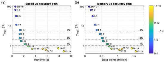
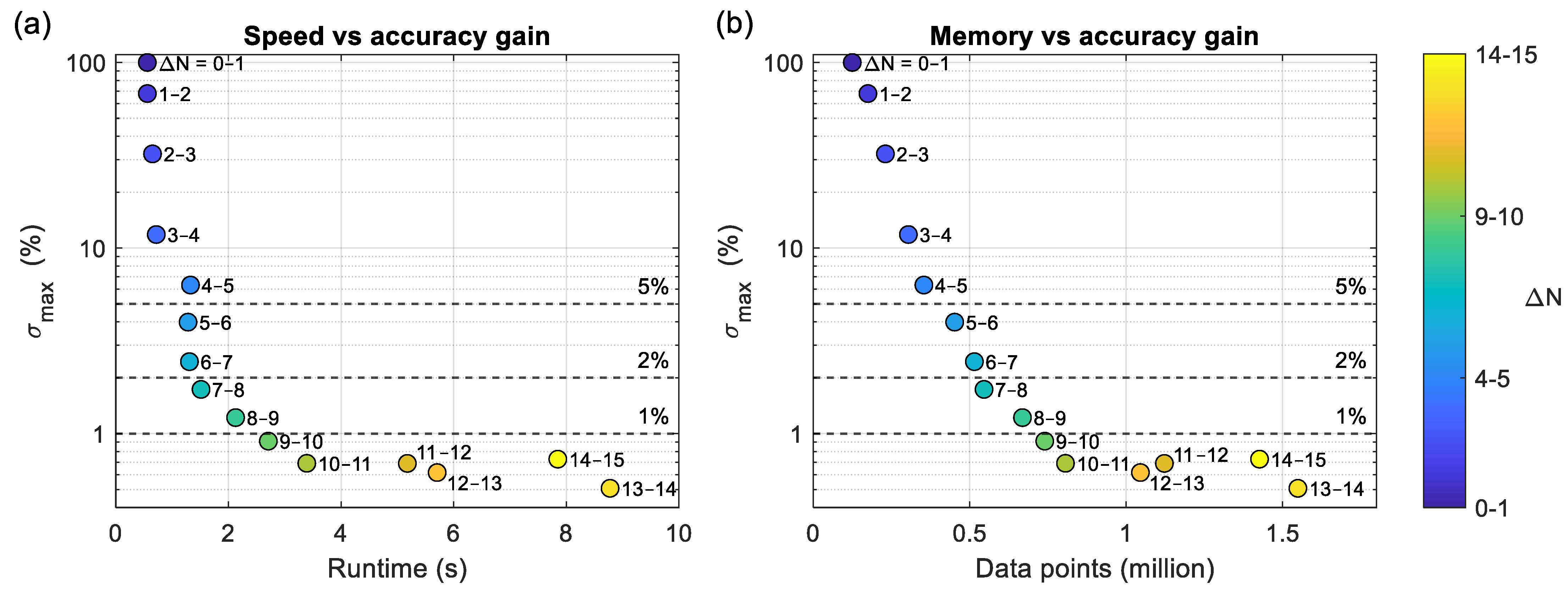
To determine a sensible number of nodes, we combine the simulation performance data from Figure 14a,c against the accuracy gain from Figure 11b to generate two Pareto fronts, as shown in Figure 15. In Figure 15a,b, a sharp bend in the performance trend is found where ΔN increases from 10–11 to 11–12. The location of this bend correlates to the change in stiffness regime as seen in Figure 14. Experimenting with different ODE solvers reveals that the exact bend point varies slightly based on the chosen solver. Therefore, a more robust approach is to define a convergence threshold. Using eight nodes keeps the convergence metric σmax below the 2% threshold while requiring less than 2 s to run. Therefore, we recommend eight nodes for most airborne wind energy applications. If speed needs to be prioritised for large-scale parameter sweeps, then six nodes can be used, which provides a small speed improvement while still keeping σmax below 5%.
Figure 15.
Pareto fronts showing the impact of increasing tether node counts on (a) runtime and (b) memory usage.
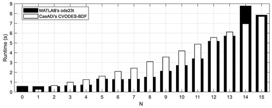
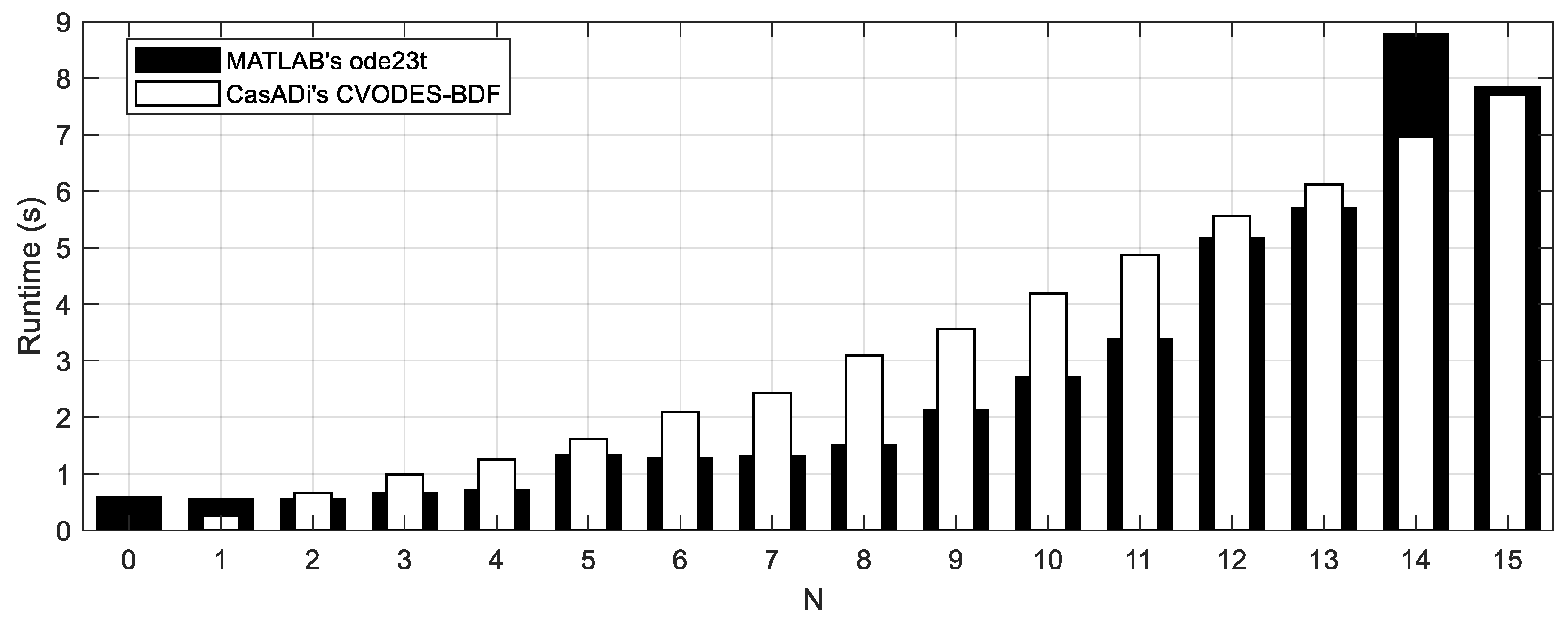
For further performance benchmarking, the runtime of ode23t is compared against the high-performance solver CVODES with backward differentiation (BDF) [34]—implemented in MATLAB using the optimisation package CasADi 3.8.1 [35]. Note that both solvers make use of the C-code generation capability mentioned above to speed up the right-hand-side evaluation of the differential equations. Figure 16 shows their runtimes. CasADi performs slightly better on either extreme (very low or very high number of nodes), although any performance difference in either direction is small and can be attributed to the authors’ coding practices. Achieving a similar speed to CVODES-BDF indicates that the performance figures discussed above are representative of what can be achieved in airborne wind energy simulation when the appropriate tether discretisation level and solver choice are in place.
Figure 16.
Runtime of the manoeuvre in Figure 13 using ode23t and CVODES-BDF solvers.
5. Conclusions
We have presented a successive difference metric to quantify the gain in simulation accuracy from adding more tether nodes in airborne wind energy systems. This accuracy gain is compared against computation cost, revealing that using between six and eight nodes is sufficient. Going beyond eight nodes can be considered excessive, as doing so incurs significant computation cost for a minuscule improvement in accuracy. Therefore, the conservative choices of 10–20 nodes in the literature can be relaxed. Doing so on a large scale can significantly reduce the computation cost of future AWES studies.
Author Contributions
Conceptualisation, D.H.N.; methodology, D.H.N.; software, D.H.N. and E.O.; validation, D.H.N. and E.O.; formal analysis, D.H.N.; investigation, D.H.N.; resources, E.O.; data curation, D.H.N.; writing—original draft preparation, D.H.N.; writing—review and editing, E.O.; visualisation, D.H.N.; supervision, D.H.N.; project administration, D.H.N.; funding acquisition, D.H.N. All authors have read and agreed to the published version of the manuscript.
Funding
Duc H. Nguyen is supported by the UK Engineering and Physical Sciences Research Council (EPSRC), grant number EP/Y014545/1. Espen Oland is part of the 3D-CIRCULAR project, which has received funding from the European Health and Digital Executive Agency under the Grant Agreement No 101226256. The contents of this publication are the sole responsibility of the authors and do not necessarily reflect the opinion of the European Union.
Data Availability Statement
The simulation model is proprietary and is not available to the public. The aerodynamic data of the model can be found in Reference [28].
Acknowledgments
The authors used the large language model Claude Sonnet 4.6 by Anthropic to help analyse the trim data and derive the convergence metric presented in Section 4.1. The authors have reviewed and edited the output and take full responsibility for the content of this publication.
Conflicts of Interest
The authors declare no conflicts of interest. The funders had no role in the design of the study; in the collection, analyses, or interpretation of data; in the writing of the manuscript; or in the decision to publish the results.
Appendix A. Further Details on the Tether Model
This section provides further details on the forces acting on the lumped mass tether model. As a reminder, the tether is discretised into N free nodes between the winch and the kite, resulting in N + 1 segments.
Gravitational force acts at the centre of each segment. The segment mass is calculated by multiplying the tether’s natural (unstretched) volume by the tether density, then dividing by the number of segments (equal to N + 1). The unstretched length is used as the indicator of tether length because stretching a segment cannot create mass, so the mass between two adjacent nodes remains constant regardless of elongation.
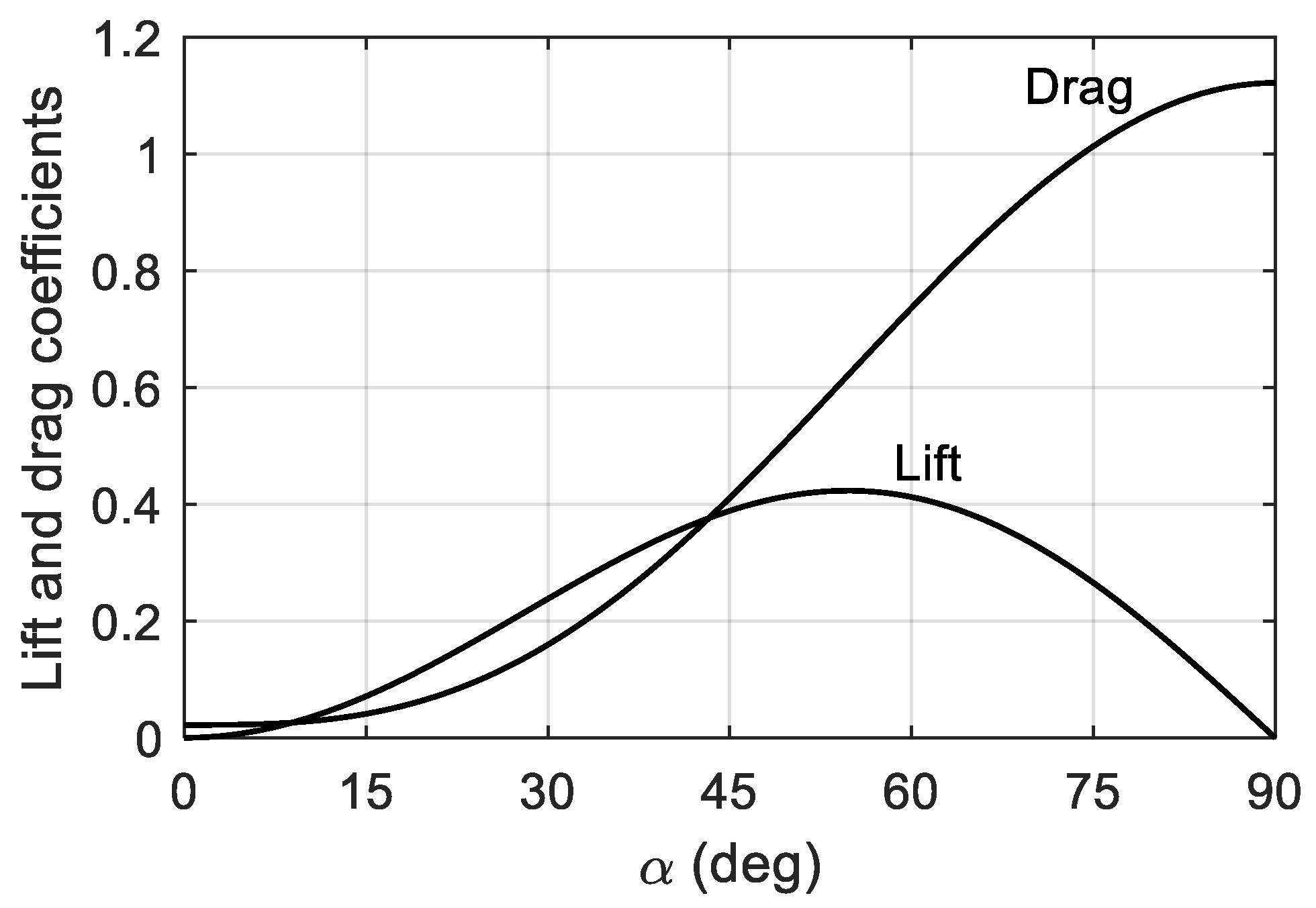
Aerodynamic forces also act at the centre of each segment and are decomposed into lift and drag. The lift and drag coefficients are developed from crossflow principle for circular cylinders (see pages 3–11 of [36]), which are reproduced by Equations (A1) and (A2):
where the 0.02 constant models skin friction drag. The coefficients are shown in Figure A1.
CL = 1.1 sin2 α cos α
CD = 1.1 sin3 α + 0.02
Figure A1.
Hoerner’s lift and drag coefficients.
Lastly, the elastic force is modelled by spring–damper elements. The spring stiffness k can be calculated from the material’s Young’s modulus E = 1.55 × 10¹¹ N/m2, segment natural length l0, and cross-sectional area A = πR2:
where R = 2 mm. When 15 tether nodes are used, each segment has length 500/16 = 31.25 m, giving a segment stiffness of ki = 62,329 Nm−1 and an overall stiffness of
Note that the whole-tether stiffness is not dependent on the number of segments because the springs are connected in series.
The damping coefficient is artificially set to 4.47 Nsm−1 to ensure numerical convergence for the differential equation solver and prevent excessive high-frequency oscillation. Changing the damping coefficient has no impact on the trim solution, which is the focus of this work. For dynamic simulation, it is possible to bypass the damping issue by ignoring the segments’ inertia and transient vibration using a quasi-steady approach presented in [37]. The performance gain can be significant. However, the authors believe such a method should only be deployed on thin and light tethers, which are more common in groundgen AWES as opposed to flygen.
The sum of all forces above gives the total force on each segment, which is distributed equally to the two adjacent nodes. The node’s acceleration is calculated by Newton’s second law, specifically by adding up the forces from the two adjacent segments, then dividing by the node mass. Each node, therefore, is represented by six states: three states for the node accelerations in 3D space, and another three states for node velocities. Integrating these six states gives the node location in the Earth’s 3D coordinates.
References
- Cherubini, A.; Papini, A.; Vertechy, R.; Fontana, M. Airborne Wind Energy Systems: A review of the technologies. Renew. Sustain. Energy Rev. 2015, 51, 1461–1476. [Google Scholar] [CrossRef] [Scilit]
- Pereira, A.F.C.; Sousa, J.M.M. A Review on Crosswind Airborne Wind Energy Systems: Key Factors for a Design Choice. Energies 2023, 16, 351. [Google Scholar] [CrossRef] [Scilit]
- Khurshid, Y.; Paul, P.; Elhesasy, M.; Ali, B.; Kamra, M.M.; Okasha, M.; Dief, T.N. From inception to commercialization: A systematic review of airborne wind energy systems. Sustain. Energy Technol. Assess. 2025, 83, 104623. [Google Scholar] [CrossRef] [Scilit]
- Ahrens, U.; Diehl, M.; Schmehl, R. Airborne Wind Energy, 1st ed.; Springer Berlin: Heidelberg, Germany, 2013. [Google Scholar]
- Schmehl, R. Airborne Wind Energy—Advances in Technology Development and Research; Springer: Singapore, 2018. [Google Scholar]
- Williams, P.; Lapthorne, P.; Trivailo, P. Circularly-Towed Lumped Mass Cable Model Validation from Experimental Data. In Proceedings of the AIAA Modeling and Simulation Technologies Conference and Exhibit, Keystone, Colorado, 21–24 August 2006. [Google Scholar]
- Williams, P.; Lansdorp, B.; Ockels, W. Nonlinear Control and Estimation of a Tethered Kite in Changing Wind Conditions. J. Guid. Control Dyn. 2008, 31, 793–799. [Google Scholar] [CrossRef] [Scilit]
- Zanon, M.; Gros, S.; Andersson, J.; Diehl, M. Airborne Wind Energy Based on Dual Airfoils. IEEE Trans. Control Syst. Technol. 2013, 21, 1215–1222. [Google Scholar] [CrossRef] [Scilit]
- Sánchez-Arriaga, G.; Pastor-Rodríguez, A.; Sanjurjo-Rivo, M.; Schmehl, R. A lagrangian flight simulator for airborne wind energy systems. Appl. Math. Model. 2019, 69, 665–684. [Google Scholar] [CrossRef] [Scilit]
- Sánchez, G. Dynamics and Control of Single-Line Kites. Aeronaut. J. 2006, 110, 615–621. [Google Scholar] [CrossRef] [Scilit]
- Gros, S.; Diehl, M. Modeling of Airborne Wind Energy Systems in Natural Coordinates. In Airborne Wind Energy; Ahrens, U., Diehl, M., Schmehl, R., Eds.; Springer: Berlin/Heidelberg, Germany, 2013; pp. 181–203. [Google Scholar]
- Erhard, M.; Strauch, H. Flight control of tethered kites in autonomous pumping cycles for airborne wind energy. Control Eng. Pract. 2015, 40, 13–26. [Google Scholar] [CrossRef] [Scilit]
- Fechner, U.; van der Vlugt, R.; Schreuder, E.; Schmehl, R. Dynamic model of a pumping kite power system. Renew. Energy 2015, 83, 705–716. [Google Scholar] [CrossRef] [Scilit]
- Malz, E.C.; Koenemann, J.; Sieberling, S.; Gros, S. A reference model for airborne wind energy systems for optimization and control. Renew. Energy 2019, 140, 1004–1011. [Google Scholar] [CrossRef] [Scilit]
- Licitra, G.; Koenemann, J.; Bürger, A.; Williams, P.; Ruiterkamp, R.; Diehl, M. Performance assessment of a rigid wing Airborne Wind Energy pumping system. Energy 2019, 173, 569–585. [Google Scholar] [CrossRef] [Scilit]
- De Schutter, J.; Leuthold, R.; Bronnenmeyer, T.; Malz, E.; Gros, S.; Diehl, M. AWEbox: An Optimal Control Framework for Single- and Multi-Aircraft Airborne Wind Energy Systems. Energies 2023, 16, 1900. [Google Scholar] [CrossRef] [Scilit]
- Vinha, S.; Fernandes, G.M.; Fernandes, M.C.R.M.; Fontes, F.A.C.C. Motion Primitives and Control on a Spherical Surface with Application to Tethered Aircraft. In Proceedings of the CEAS EuroGNC 2026, Madrid, Spain, 5–7 May 2026. [Google Scholar]
- Vertovec, N.; Ober-Blöbaum, S.; Margellos, K. Safety-Aware Hybrid Control of Airborne Wind Energy Systems. J. Guid. Control Dyn. 2024, 47, 326–338. [Google Scholar] [CrossRef] [Scilit]
- Crismer, J.B.; Haas, T.; Duponcheel, M.; Winckelmans, G. Large-eddy simulation of airborne wind energy systems flying in turbulent wind using model predictive control. Wind Energ. Sci. 2026, 11, 2669–2694. [Google Scholar] [CrossRef] [Scilit]
- Rapp, S.; Schmehl, R. Enhancing Resilience of Airborne Wind Energy Systems Through Upset Condition Avoidance. J. Guid. Control Dyn. 2021, 44, 251–265. [Google Scholar] [CrossRef] [Scilit]
- Heydarnia, O.; Wauters, J.; Lefebvre, T.; Crevecoeur, G. Optimal Path Planning of Airborne Wind Energy Systems with a Flexible Tether. J. Guid. Control Dyn. 2025, 48, 2881–2888. [Google Scholar] [CrossRef] [Scilit]
- Yu, K.; Nguyen, D.H.; Castro-Fernández, I.; DeLosRíos-Navarrete, F.; González-García, J.; Lowenberg, M.H.; Sánchez-Arriaga, G. Trim analysis of a three-line kite airborne wind Energy system using bifurcation analysis. In Proceedings of the CEAS EuroGNC 2026, Madrid, Spain, 5–7 May 2026. [Google Scholar]
- Williams, P.; Lansdorp, B.; Ockesl, W. Optimal Crosswind Towing and Power Generation with Tethered Kites. J. Guid. Control Dyn. 2008, 31, 81–93. [Google Scholar] [CrossRef] [Scilit]
- Eijkelhof, D.; Schmehl, R. Six-degrees-of-freedom simulation model for future multi-megawatt airborne wind energy systems. Renew. Energy 2022, 196, 137–150. [Google Scholar] [CrossRef] [Scilit]
- Nguyen, D.H.; Lowenberg, M.H.; Oland, E. Trimming a rigid-wing airborne wind system for coordinated circular flights. Wind Energy Sci. 2026, 11, 285–298. [Google Scholar] [CrossRef] [Scilit]
- Nguyen, D.H.; Lowenberg, M.H.; Oland, E. Improving Power Generation in Rigid-Wing Groundgen Airborne Wind Energy Systems Using Feedback Control—A Parametric Study. Wind Energy 2026, 29, e70109. [Google Scholar] [CrossRef] [Scilit]
- Mohammed, T.; Busk, J.; Oland, E.; Fagiano, L. Large-Scale Reverse Pumping for Rigid-Wing Airborne Wind Energy Systems. J. Guid. Control Dyn. 2024, 47, 1748–1758. [Google Scholar] [CrossRef] [Scilit]
- Mohammed, T.M.H. Automatic Control Solutions to Enhance the Reliability of Airborne Wind Energy Systems; Polytechnic University of Milan: Milan, Italy, 2024. [Google Scholar]
- Rapp, S.; Schmehl, R.; Oland, E.; Haas, T. Cascaded Pumping Cycle Control for Rigid Wing Airborne Wind Energy Systems. J. Guid. Control Dyn. 2019, 42, 2456–2473. [Google Scholar] [CrossRef] [Scilit]
- Trevisi, F.; Croce, A.; Riboldi, C.E.D. Flight Stability of Rigid Wing Airborne Wind Energy Systems. Energies 2021, 14, 7704. [Google Scholar] [CrossRef] [Scilit]
- Nguyen, D.H.; Porta Ko, A.; Tveide, T.; Lowenberg, M.H.; Oland, E. Controlling rigid-wing airborne wind energy systems during circular flight without exact path following. Wind Energy Sci. 2026, 11, 2987–3013. [Google Scholar] [CrossRef] [Scilit]
- Coetzee, E.; Krauskopf, B.; Lowenberg, M.H. The Dynamical Systems Toolbox: Integrating AUTO into Matlab. In Proceedings of the 16th US National Congress of Theoretical and Applied Mechanics, State College, PA, USA, 27 June–2 July 2010. [Google Scholar]
- Doedel, E.J.; Oldeman, B.E. AUTO-07P GitHub Depository. Available online: https://Github.com/auto-07p/auto-07p (accessed on 6 August 2026).
- Hindmarsh, A.C.; Brown, P.N.; Grant, K.E.; Lee, S.L.; Serban, R.; Shumaker, D.E.; Woodward, C.S. SUNDIALS: Suite of nonlinear and differential/algebraic equation solvers. ACM Trans. Math. Softw. 2005, 31, 363–396. [Google Scholar] [CrossRef] [Scilit]
- Andersson, J.A.E.; Gillis, J.; Horn, G.; Rawlings, J.B.; Diehl, M. CasADi: A software framework for nonlinear optimization and optimal control. Math. Program. Comput. 2019, 11, 1–36. [Google Scholar] [CrossRef] [Scilit]
- Hoerner, S.F. Fluid-Dynamic Drag: Practical Information on Aerodynamic Drag and Hydrodynamic Resistance, 2nd ed.; Hoerner Fluid Dynamics: Bakersfield, CA, USA, 1965. [Google Scholar]
- Williams, P. Cable Modeling Approximations for Rapid Simulation. J. Guid. Control Dyn. 2017, 40, 1779–1788. [Google Scholar] [CrossRef] [Scilit]

Disclaimer/Publisher’s Note: The statements, opinions and data contained in all publications are solely those of the individual author(s) and contributor(s) and not of MDPI and/or the editor(s). MDPI and/or the editor(s) disclaim responsibility for any injury to people or property resulting from any ideas, methods, instructions or products referred to in the content. |
© 2026 by the authors. Licensee MDPI, Basel, Switzerland. This article is an open access article distributed under the terms and conditions of the Creative Commons Attribution (CC BY) license.