Deep Contrastive BiGRU Network for Cross-Domain Aero-Engine Fault Detection

Abstract

Cross-domain aero-engine fault detection is challenging because vibration signals collected under different operating conditions exhibit substantial distribution shifts. Existing diagnostic models mainly focus on feature extraction or global domain alignment, often overlooking fault class separability near decision boundaries. This study proposes a perturbation-enhanced deep contrastive learning bidirectional gated recurrent unit framework (DCL-BiGRU) for unsupervised cross-domain fault detection. A shared BiGRU encoder captures bidirectional temporal dependencies, while deep contrastive learning improves intra-class compactness and inter-class separation. A controlled perturbation strategy strengthens robustness to noise and feature variation, and maximum classifier discrepancy guides uncertain target samples toward reliable source-supported class regions. Experiments on two laboratory datasets and one practical aero-engine dataset show accuracies of 95.62% and 92.48% for two transfer tasks, with a mean accuracy of 94.05%. The method outperforms DCL, BiGRU, TCA, JDA, MNN, and DANN approaches, confirming improved domain alignment, class discrimination, and diagnostic robustness under practical conditions.

1. Introduction

Aircraft engine fault diagnosis is an essential requirement in aerospace systems because it directly supports flight safety, reduces unexpected downtime, and assists condition-based maintenance planning. Due to the highly complex structure and safety-critical nature of aircraft engines, identifying abnormal conditions quickly and accurately remains a challenging task [1,2]. Since engine components operate under variable speed, load, temperature, and environmental conditions, conventional rule-driven or threshold-based diagnosis methods often fail to provide reliable results, especially when sensor noise and uncertainty are present [3,4].

Recent progress in learning-based diagnostic models has greatly enhanced fault detection in rotating machinery [5,6]. Compared with manual inspection and traditional statistical approaches, these methods can automatically learn useful fault-related representations from raw monitoring signals [7,8]. In this area, CNN-based diagnostic models [9,10], RNN-based models [11], and LSTM-based architectures have been extensively used for machinery health monitoring [12,13]. Nevertheless, most of these approaches were developed under the assumption that training and testing samples share similar distributions, which is difficult to satisfy in real aircraft engine operating environments. Differences between the data used for model training and the data encountered during testing often lead to domain shift, which has made transfer learning, especially unsupervised domain adaptation (UDA), an important strategy for cross-domain diagnosis [14,15]. UDA learns transferable representations so that knowledge obtained from annotated source samples can be applied to target samples without labels. This is especially useful in industrial applications, where collecting labeled fault samples from real engines is costly, labor-intensive, and sometimes impractical [16,17]. Several UDA methods have been introduced for cross-domain diagnosis. Traditional shallow approaches, such as Transfer Component Analysis (TCA) [18] and Joint Distribution Adaptation (JDA) [19], reduce domain differences by projecting data into a shared latent space. However, their ability to learn complex and high-level fault characteristics is limited. Deep adaptation methods, including Deep Adaptation Networks (DANs) [20], Domain-Adversarial Neural Networks (DANNs) [21], and Conditional Adversarial Domain Adaptation (CDAN) [22], have improved domain alignment performance by integrating deep feature learning with adaptation strategies. Even so, most existing alignment methods emphasize domain-level matching while giving limited attention to the placement of target samples near decision regions [23,24]. To overcome this limitation, MCD uses two task-specific classifiers to guide adaptation around decision boundaries [25]. MCD employs two independent task classifiers to expose target-domain samples that are not yet well aligned with the source-supported feature region by increasing the disagreement between their predictions. Then, the feature extractor is optimized to reduce this disagreement, forcing target features to move closer to the source-supported class regions [26,27]. Despite the progress achieved by the above methods, several limitations remain in cross-domain aero-engine fault diagnosis. Conventional CNN, RNN, LSTM, and BiGRU-based diagnostic models mainly improve feature extraction, but they generally assume that the training and testing data follow similar distributions. Their performance can therefore decrease significantly when vibration signals are collected under different rotational speeds, loads, sampling conditions, or sensor environments. Shallow transfer learning methods, such as TCA and JDA, reduce statistical distribution differences through latent-space projection, but their limited nonlinear representation capability makes it difficult to model complex temporal fault characteristics. Deep adaptation approaches, including DANs, DANNs, and CDANs, provide stronger nonlinear alignment; however, they primarily focus on matching global or conditional domain distributions. Such alignment may place target samples close to inappropriate source class regions when class boundaries are not explicitly considered. MCD improves upon global domain alignment by using the disagreement between two task-specific classifiers to identify target samples located near uncertain decision boundaries. Nevertheless, the original MCD framework mainly addresses boundary-aware adaptation and does not explicitly optimize the temporal structure, class-wise compactness, and perturbation robustness required for noisy aero-engine vibration signals. Similarly, standalone contrastive learning methods improve sample discrimination but do not necessarily resolve cross-domain decision boundary mismatch, while a standalone BiGRU can capture bidirectional temporal dependencies but cannot guarantee domain-invariant feature alignment. The proposed DCL-BiGRU framework differs from these previous studies by jointly addressing temporal representation, class-level discrimination, robustness, and boundary-aware domain adaptation within a unified model. Specifically, BiGRU captures bidirectional temporal dependencies in raw vibration sequences; deep contrastive learning reduces intra-class variation and enlarges inter-class margins; the perturbation strategy improves resistance to noise and unstable feature changes; and the MCD mechanism aligns unlabeled target samples with reliable source-supported fault regions according to classifier decision boundaries. Consequently, the proposed method does not merely reduce the overall source–target distribution gap; it also preserves fault category structure and improves the stability of cross-domain classification under practical operating variations.

Motivated by this idea, this study introduces an enhanced aircraft engine fault diagnosis framework that combines deep contrastive learning with a BiGRU network and embeds it within a noise-tolerant adaptation framework. In the proposed framework, BiGRU is adopted to model sequential vibration signals by extracting information from both forward and backward temporal directions. This bidirectional learning ability allows the network to capture more complete fault-related patterns, which is important for recognizing short-duration and transient fault behaviors [28,29,30]. In addition, the perturbation strategy is embedded into the MCD-based adversarial learning process to improve training stability, strengthen feature robustness, and reduce the risk of overfitting or feature degradation during domain adaptation [31]. To evaluate the proposed method, three datasets are used for validation: D1 and D2 from laboratory test platforms, and D3 from a practical aero-engine test system. The proposed DCL-BiGRU model is compared with representative feature learning and unsupervised domain adaptation approaches, including DCL, BiGRU, TCA, JDA, MNN, DANN, the original MCD framework, and CDAN approaches. All approaches are evaluated using a unified 550-point raw signal input pipeline to ensure a controlled comparison. The experimental outcomes, supported by quantitative evaluation, qualitative analysis, and t-SNE feature visualization, confirm that the proposed method delivers more accurate fault recognition, clearer class-wise feature separation, and stronger cross-domain representation consistency.

Different from existing MCD and contrastive domain adaptation methods, the proposed framework does not regard BiGRU, contrastive learning, perturbation, or MCD as individually novel components. Its methodological contribution lies in their coupled optimization. Conventional MCD primarily identifies uncertain target samples through disagreement between two task-specific classifiers and subsequently adapts the feature generator by minimizing this discrepancy. It does not explicitly impose supervised contrastive class geometry on the source representation or require the adaptation process to remain consistent under controlled perturbations. In the proposed framework, a shared BiGRU first captures bidirectional temporal dependencies, while supervised contrastive learning establishes compact intra-class and separated inter-class representations. The MCD mechanism then performs boundary-aware target adaptation within this discriminative feature space. In addition, perturbation is incorporated into source classification, contrastive representation learning, and target-domain discrepancy estimation. Consequently, source discrimination, contrastive geometry, perturbation robustness, and target-domain alignment are optimized jointly rather than as independent or sequential procedures. Based on the limitations identified above, the main contributions of this paper are summarized as follows:

• A new domain-adaptive DCL-BiGRU framework is proposed for aircraft engine fault diagnosis, combining temporal feature extraction with cross-domain feature alignment.
• A perturbation-coupled optimization strategy is developed in which feature disturbance is consistently incorporated into source classification, contrastive representation learning, and target-domain classifier discrepancy estimation. Rather than treating perturbation as an independent augmentation step, the proposed formulation jointly optimizes class discrimination, feature robustness, and boundary-aware domain adaptation under controlled feature variation.
• Extensive experiments on laboratory and practical aircraft engine datasets verify that the proposed method outperforms several baseline and advanced transfer learning models.

The rest of the paper is structured as follows: Section 2 presents the proposed methodology, Section 3 describes the experimental setup, Section 4 discusses the results, and Section 5 concludes the study.

2. Conceptual Foundations of the DCL-BiGRU Method

2.1. Contrastive Domain Adaptation for Fault Diagnosis

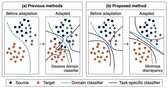
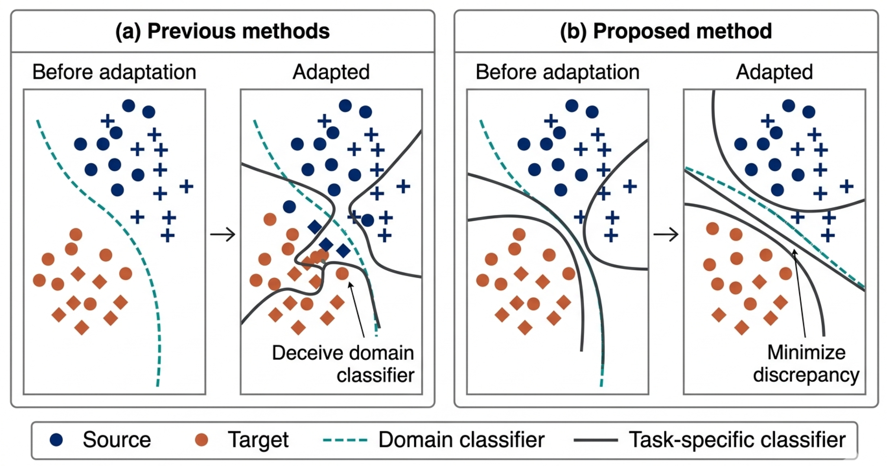
Figure 1 compares conventional domain adaptation approaches with the proposed decision boundary-aware adaptation strategy. In earlier methods, the main objective was usually to reduce the overall distribution difference between the source and target domains by using a domain classifier. Although this process can make samples from both domains appear closer in the feature space, it may not correctly preserve the category structure. As a result, some target samples may be moved near incorrect class regions, causing class overlap and reducing diagnostic reliability.

Figure 1. Comparison between existing domain adaptation approaches and the proposed contrastive feature alignment strategy.

In contrast, the proposed strategy aligns target features while considering their interaction with class-dependent decision regions. Instead of only confusing a domain classifier, the model uses task-related classifiers to identify uncertain target samples located near boundary regions. By minimizing the discrepancy between these classifiers, the target-domain features are gradually guided toward the appropriate source-domain class regions.

This strategy improves class separability while reducing the domain gap. Therefore, the adapted feature space becomes more discriminative and stable, enabling the proposed model to achieve more reliable cross-domain aircraft engine fault diagnosis under changing operating conditions.

2.2. Deep Contrastive Learning and BiGRU Integration

BiGRU is adopted not only to extract temporal information but also to support discriminative feature learning. Since aircraft engine vibration signals are sequential, BiGRU captures fault patterns from both forward and backward directions [32]. Unlike traditional RNNs, which may suffer from gradient vanishing or exploding, GRU-based structures improve stability through gating mechanisms [33,34]. In this framework, the BiGRU encoder converts raw vibration signals into bidirectional temporal features. Deep contrastive learning then pulls features of the same fault class closer and pushes different classes farther apart. With perturbation and projection operations, the model learns robust and class-separable representations for cross-domain fault diagnosis.

The integration process can be expressed as follows:

$$\begin{array}{cc}\hfill H^d& =B_{\overleftrightarrow{\varphi }}\left(X^d\right),\hfill \\ \hfill z^d& =\mathsf{\Gamma }\left(H^d\right),d\in \{s,t\},\hfill \\ \hfill q^d& =\frac{\mathsf{\Pi }\left(p\left(z^d\right)\right)}{{\Vert \mathsf{\Pi }(p(z^d))\Vert }_{ 2}}.\hfill \end{array}$$

(1)

where $d\in \left\{s,t\right\}$ denotes the source domain and target domain, respectively, $X^d$ is the input sample set of domain d, $B_{\overleftrightarrow{\varphi }}$ denotes the shared BiGRU encoder parameterized by $\varphi$, $H^d$ is the hidden representation generated by the BiGRU encoder, $\mathsf{\Gamma }$ denotes the feature mapping or aggregation function, $z^d$ is the encoder output feature, $q^d$ denotes the projected and normalized embeddings in the contrastive space, P denotes the perturbation operator, and $\mathsf{\Pi }$ denotes the projection head used for deep contrastive learning.

$$\begin{array}{cc}\hfill z_j^d& =G_B\left(x_j^d\right)=\left[{\overrightarrow{h}}_{L,j}^d;{\overleftarrow{h}}_{1,j}^d\right],d\in \{s,t\},\hfill \\ \hfill u_j^d& =P\left(p\left(z_j^d\right)\right),\hfill \\ \hfill {\hat{u}}_j^d& ={\displaystyle \frac{u_j^d}{{∥u_j^d∥}_2}}.\hfill \end{array}$$

(2)

where $u_j^d$ and ${\hat{u}}_j^d$ denote the projected and normalized embeddings in the contrastive space, $G_B$ denotes the shared BiGRU generator, ${\overrightarrow{h}}_{L,j}^d$ and ${\overleftarrow{h}}_{1,j}^d$ are the forward and backward hidden states, and $[;]$ denotes the concatenation operation. These equations show that the input sequence is first encoded by BiGRU to capture bidirectional temporal information, then transformed into a projected embedding, and finally normalized for contrastive learning.

Equation (1) illustrates how source and target inputs are transformed by BiGRU into normalized contrastive embeddings. Equation (2) explains the sample-wise process, where each vibration signal is encoded, projected, perturbed, and normalized for contrastive learning. Unlike earlier formulations, these features are directly optimized to improve same-class compactness and different-class separation for cross-domain fault diagnosis.

2.3. Differences from Existing Contrastive Learning Frameworks

Conventional contrastive learning approaches generally learn representations by maximizing agreement between augmented views of the same sample or by reducing the distance between samples belonging to the same labeled class. Although such methods can improve feature discrimination, they are commonly developed for single-domain representation learning and do not explicitly consider the distribution shift between labeled source data and unlabeled target data. They also do not directly determine whether target samples are located near unreliable task-specific decision boundaries.

The proposed framework differs from these approaches in four essential aspects. First, contrastive learning is not employed as an independent pretraining stage; it is jointly optimized with source-domain classification and target-domain adaptation through a shared BiGRU encoder and projection head. The contrastive objective organizes the labeled source representations by increasing intra-class compactness and inter-class separation, thereby establishing a discriminative class structure that supports subsequent target adaptation.

Second, unlabeled target samples are not assigned directly to contrastive positive pairs using potentially unreliable target labels. Instead, two task-specific classifiers measure their prediction discrepancy. Samples producing high disagreement are treated as being close to uncertain decision regions, and the shared encoder is updated to move their features toward regions supported by the source-domain class structure. This reduces the risk of error propagation that may arise when inaccurate target pseudo-labels are used to construct positive and negative contrastive pairs.

Third, the perturbation operator is coupled with all major learning branches. Source classification is performed on perturbed features, contrastive embeddings are generated after feature transformation and perturbation, and target-domain discrepancy is calculated using perturbed target representations. Therefore, the model is encouraged to maintain class discrimination and domain alignment under controlled feature variation rather than only under clean representations.

Fourth, the model uses an alternating optimization mechanism rather than a simple sequential connection of modules. During classifier optimization, the shared encoder is fixed and the two classifiers enlarge their disagreement on target samples while retaining source-domain classification performance. During encoder optimization, the classifiers are fixed and the BiGRU encoder and projection head reduce target discrepancy while maintaining source supervision and contrastive class geometry. Consequently, temporal modeling, contrastive discrimination, perturbation robustness, and boundary-aware adaptation mutually constrain the same feature space.

It should be emphasized that the distinction from straightforward end-to-end multi-task training does not arise from the weighted addition of the individual loss terms. Rather, it arises from the parameter-specific alternating optimization. The two classifiers and the shared representation are not optimized simultaneously with the same objective direction. The classifiers are first optimized to expose uncertain target samples by increasing their discrepancy, whereas the encoder and projection head are subsequently optimized in the opposite direction to reduce this discrepancy while preserving the source-supervised contrastive structure. Consequently, the contrastive and discrepancy objectives play different roles at different optimization stages rather than simply contributing simultaneously to a single end-to-end objective.

These differences provide two principal technical advantages: the source feature space becomes compact and class-separable before target alignment, while the target features are adapted according to task-specific decision boundaries rather than global distribution similarity alone. In addition, perturbation-consistent optimization improves resistance to vibration noise and operating condition variation. Thus, the proposed method represents a coupled contrastive domain adaptation formulation rather than a simple aggregation of independently trained modules.

3. Design of the DCL-BiGRU Diagnosis Model

This section describes the proposed DCL-BiGRU framework for cross-domain aircraft engine fault diagnosis. The model focuses on improving the discriminative quality of the learned feature space. Under domain shift, reliable diagnosis requires both domain alignment and clear separation among fault categories. Therefore, the proposed method integrates BiGRU, deep contrastive learning, MCD-based adaptation, and a perturbation strategy. BiGRU extracts bidirectional temporal patterns from aircraft engine vibration signals. Deep contrastive learning enhances intra-class compactness and inter-class separation, while MCD aligns target features around task-specific decision boundaries. Perturbation further improves robustness, enabling the model to learn stable and domain-invariant fault representations.

3.1. Boundary-Aware Adaptation via MCD

In the proposed DCL-BiGRU model, domain adaptation is designed beyond simple source–target distribution matching. The method focuses on the location of target-domain samples with respect to fault class decision boundaries. This is important because global alignment may still leave target samples in uncertain or overlapping class regions. Such ambiguity is common in aircraft engine vibration data due to noise, multi-modal distributions, and changing operating conditions.

Therefore, reducing the domain discrepancy alone cannot guarantee accurate fault classification. The learned features must also preserve class separability while becoming domain-invariant. For this purpose, maximum classifier discrepancy (MCD) is introduced as a boundary-aware adaptation strategy.

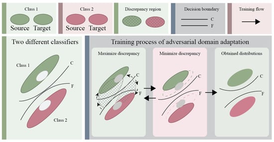
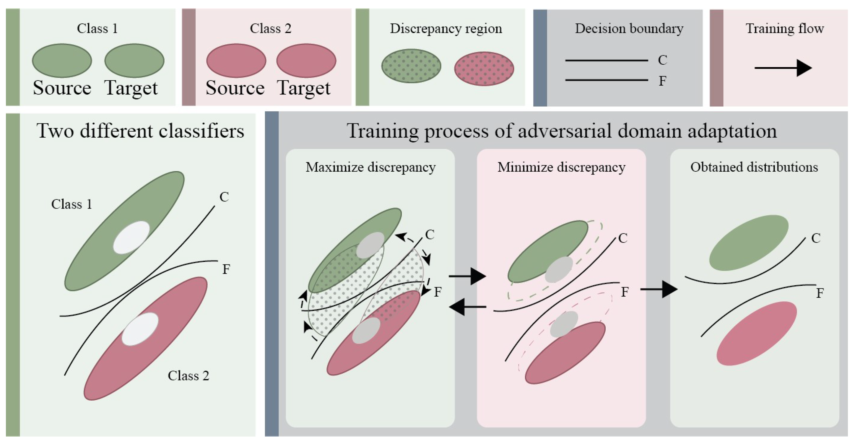
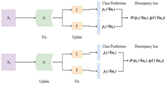
Figure 2 illustrates that two task-specific classifiers, C and F, observe the same feature space from different decision perspectives. During training, their disagreement highlights target samples located near unreliable boundary areas. The feature extractor is then optimized to move these target features toward more confident class-specific regions. Thus, classifier discrepancy acts as a useful guide for improving class-level alignment and robust cross-domain diagnosis.

Figure 2. Conceptual illustration of boundary-aware adaptation in the proposed DCL-BiGRU model.

The target-domain discrepancy used in the proposed framework is defined on the perturbed target features as follows:

$$\begin{array}{cc}\hfill L_{\mathrm{disc}}^t& ={\displaystyle \frac{1}{N_t}}{\displaystyle \sum _{j=1}^{N_t}}{∥p_c\left({\tilde{z}}_j^t\right)-p_f\left({\tilde{z}}_j^t\right)∥}_1,\hfill \\ \hfill {\tilde{z}}_j^t& =p\left(z_j^t\right).\hfill \end{array}$$

(3)

where $N_t$ denotes the number of target-domain samples, $z_j^t$ is the feature representation of the j-th target-domain sample, ${\tilde{z}}_j^t$ is the perturbed feature obtained by the perturbation operator p, and $p_c$ and $p_f$ are the prediction outputs of classifiers C and F, respectively. The L1-norm is used to measure the prediction difference between the two classifiers.

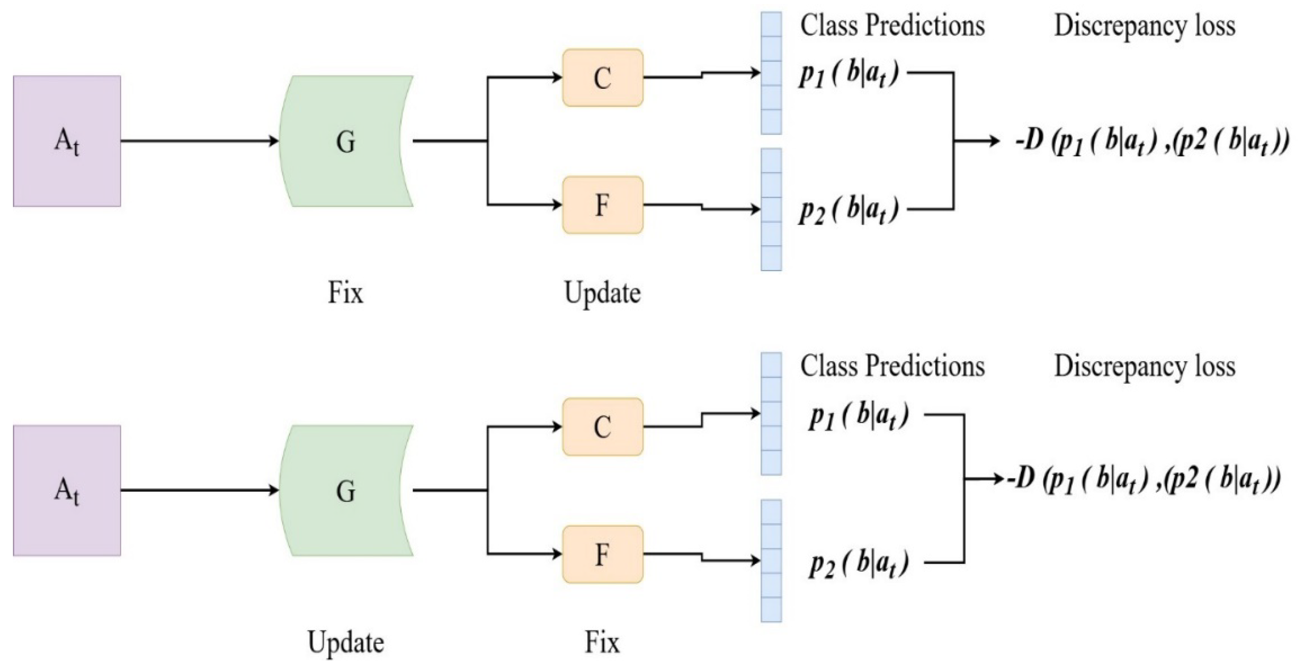
Figure 3 shows the two repeated optimization stages adopted in the proposed framework. In Step A, the feature extractor remains unchanged, while the two classifiers are trained to increase their prediction difference on target-domain data. This process helps reveal target features that are still uncertain or positioned near fault class boundaries. In Step B, the classifiers are kept constant, and the feature extractor is improved to minimize their disagreement. Through this operation, target-domain features are progressively shifted toward areas where both classifiers provide similar and confident outputs. Thus, the proposed adaptation strategy works as an iterative adjustment of target feature distribution and decision structure rather than a direct single-stage alignment between domains.

Figure 3. Alternating optimization scheme for boundary-aware discrepancy adaptation in the DCL-BiGRU framework.

Based on the above discrepancy mechanism, the adversarial optimization objectives of the proposed DCL-BiGRU model are formulated as follows:

$$\underset{C,F}{min}{L}_s+{\lambda }_c{L}_{\mathrm{dcl}}-\beta L_{\mathrm{disc}}^t,\mathrm{with}{G}_B,\mathsf{\Pi }\mathrm{fixed},$$

(4)

$$\underset{G_B,\mathsf{\Pi }}{min}{L}_s+{\lambda }_c{L}_{\mathrm{dcl}}+\beta L_{\mathrm{disc}}^t,\mathrm{with}C,F\mathrm{fixed}.$$

(5)

where $L_s$ denotes the source-domain classification loss, $L_{dcl}$ denotes the deep contrastive learning loss, $L_{disc}^t$ is the target-domain discrepancy loss defined in Equation (3), ${\lambda }_c$ is the weighting coefficient for the contrastive term, and $\beta$ controls the contribution of the discrepancy term. In Equation (4), the encoder and projection head are fixed, and the classifiers are updated so that source-domain discrimination is maintained while the target-domain discrepancy is enlarged. In Equation (5), the optimization focuses shifts to the BiGRU generator and the projection head, which are jointly updated to reduce the target-domain discrepancy while preserving source-domain classification ability and the contrastive structure of the embedding space. In this way, MCD is no longer used in isolation; it works together with deep contrastive learning so that the learned features become simultaneously boundary aware, domain adaptive, and contrastively discriminative. This joint optimization distinguishes the proposed DCL-BiGRU framework from conventional MCD-based adaptation methods by simultaneously promoting boundary-aware domain alignment, source-domain discrimination, and contrastive class separation.

3.2. Perturbation-Enhanced DCL-BiGRU Architecture

The proposed architecture is developed for a challenging cross-domain fault diagnosis task, where the extracted feature representation must support both domain transferability and strong class-level distinction. Therefore, the model is not limited to sequence feature extraction or distribution discrepancy reduction alone. Instead, the diagnostic pipeline is constructed as an integrated framework that combines a shared BiGRU encoder, deep contrastive learning, perturbation-guided feature enhancement, and MCD-based adaptation. This arrangement is intended to make vibration samples belonging to the same aircraft engine fault condition cluster more closely in the embedding space, while samples from different health states are pushed farther apart, even when the source and target domains show large distribution differences.

The perturbation operation used in this study should be distinguished from conventional input-level noise augmentation. Generic noise injection normally creates a disturbed training sample and then optimizes a single classification objective. In the proposed framework, perturbation is applied at the learned feature level and influences three interconnected objectives: First, perturbed source features are used to optimize the supervised classification loss, encouraging stable source-domain decision boundaries. Second, perturbed projected embeddings are used in the contrastive objective, encouraging samples from the same fault category to remain close under feature variation while maintaining separation from other categories. Third, perturbed target features are passed to the two task-specific classifiers when calculating classifier discrepancy, so target-domain alignment is performed under local feature disturbance rather than only on clean representations.

These three uses of perturbation are coupled through the shared BiGRU encoder and projection head. During classifier optimization, the encoder is fixed and the classifiers expose uncertain perturbed target samples by increasing their prediction disagreement while preserving source discrimination. During encoder optimization, the classifiers are fixed and the shared representation is updated to reduce discrepancy while retaining the source classification and contrastive structures. Therefore, perturbation does not constitute an independent module appended to the network; it acts as a common robustness constraint across the classification, contrastive, and adaptation objectives.

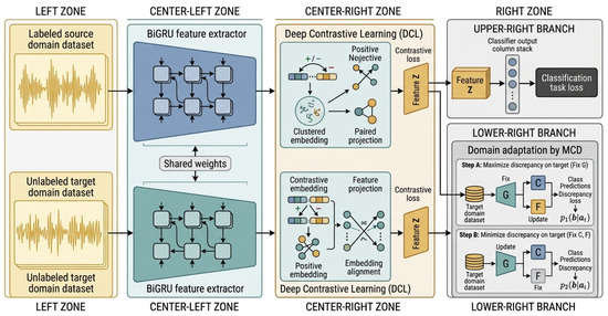
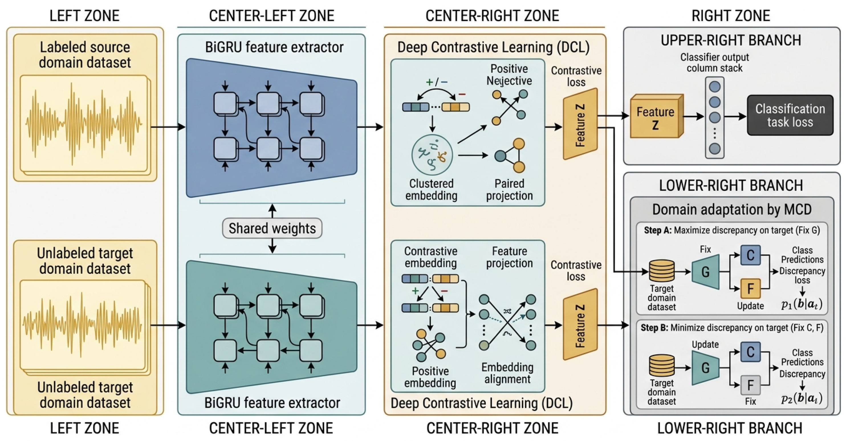
Figure 4 presents the overall framework, which can be viewed as a structured architecture with several connected functional parts. In the left part, the framework takes labeled source instances and unlabeled target instances as input. In the middle-left part, both types of data are processed by the same BiGRU feature extractor, allowing them to be represented within a shared temporal feature space. In the middle-right part, the obtained features are passed to the deep contrastive learning module, where projection and embedding refinement are performed. This component helps improve the feature distribution by making same-class representations more concentrated and different-class representations more distinguishable. In the right part, the framework separates into two learning paths: the upper classification path performs supervised learning using source-domain labels, while the lower MCD path carries out target-domain adaptation. In this way, the learned representation Z is jointly optimized for accurate fault recognition and effective cross-domain generalization.

Figure 4. Overall architecture of the perturbation-enhanced DCL-BiGRU framework for cross-domain aircraft engine fault diagnosis.

Mathematical Definition and Implementation of Perturbation

To improve robustness against measurement noise, amplitude variation, temporal misalignment, and instability of learned representations, a controlled perturbation strategy is incorporated into the proposed DCL-BiGRU framework. The perturbation is introduced at the signal, feature, and classifier levels during training. For an original vibration segment (x), the perturbed signal is expressed as follows:

$$\begin{array}{c}\multicolumn{1}{c}{{\displaystyle {\tilde{x}}_j^d\left(t\right)=a_j^d{x}_j^d(t+{\Delta }_j^d)+{ϵ}_j^d\left(t\right),d\in \{s,t\},}}\\ {\displaystyle \mathrm{where}{a}_j^d\sim \mathcal{U}(0.90,1.10),{\Delta }_j^d\sim {\mathcal{U}}_d(-10,10),{ϵ}_j^d\left(t\right)\sim \mathcal{N}\left(0,{\left(0.01{\sigma }_{x_j^d}\right)}^2\right).}\hfill \end{array}$$

(6)

Here, (a) denotes a random amplitude-scaling factor, ($\Delta$) represents a temporal shift, and $\in \left(t\right)$ is additive Gaussian noise. The perturbation parameters are sampled, where u denotes the continuous uniform distribution, ${\mathcal{U}}_d$ denotes the discrete uniform distribution, and $\sigma \left(x\right)$ is the standard deviation of the corresponding vibration segment. Therefore, the Gaussian noise magnitude corresponds to 1% of the signal standard deviation, the amplitude variation is limited to ±10%, and the maximum temporal displacement is ±10 sampling points.

$$z_j^d=G_B\left({\tilde{x}}_j^d\right),d\in \{s,t\},$$

(7)

After the perturbed vibration sequence is processed by the shared BiGRU encoder, feature-level perturbation is introduced using dropout. For a learned feature vector (z), the perturbed representation is

$${\tilde{z}}_j^d={\displaystyle \frac{m_j^d\odot z_j^d}{1-p_f}},m_{j,k}^d\sim \mathrm{Bernoulli}(1-p_f),p_f=0.30,$$

(8)

and $(\odot )$ denotes element-wise multiplication. Thus, 30% of the feature activations are randomly suppressed during training. The scaling factor ${\displaystyle \frac{1}{(1-p_f)}}$ maintains the expected activation magnitude. A dropout probability of $(p_f=0.30)$ is also applied within the classifier branches (C) and (F). Because the two task-specific classifiers have independently sampled dropout masks, they retain slightly different decision responses, which supports the MCD mechanism in identifying target samples located near uncertain class boundaries. During training, the perturbation operations are randomly regenerated for each mini-batch. Perturbed source representations are used for supervised classification and contrastive representation learning, whereas perturbed target representations are passed through classifiers (C) and (F) for discrepancy estimation. Perturbation is active only during model training and is disabled during final inference and performance evaluation. In this manner, the proposed method learns features and decision boundaries that remain stable under controlled variations without altering the class labels or introducing target-domain supervision.

The supervised classification objective on the source domain is formulated as follows:

$$\begin{array}{cc}\hfill L_s& =-{\displaystyle \frac{1}{2N_s}}{\displaystyle \sum _{j=1}^{N_s}}{\displaystyle \sum _{i=1}^n}{y}_{ji}^s\left[log{p}_{c,i}\left({\tilde{z}}_j^s\right)+log{p}_{f,i}\left({\tilde{z}}_j^s\right)\right],\hfill \\ \hfill {\tilde{z}}_j^s& =p\left(z_j^s\right).\hfill \end{array}$$

(9)

where $N_s$ denotes the number of source-domain samples, n is the number of fault classes, $y_{ji}^s$ is the label indicator of the j-th source-domain sample for class i, and $pc,i\left({\tilde{z}}_j^s\right)$ and $pf,i\left({\tilde{z}}_j^s\right)$ are the outputs of the two classifiers C and F, respectively. The term ${\tilde{z}}_j^s=p\left(z_j^s\right)$ indicates that the source-domain feature is first perturbed by the operator p before classification. Therefore, the source branch objective is not computed on a fixed feature vector, but on a perturbed representation, which helps the model learn source-domain decision boundaries that are more stable under feature variation. This is especially useful in aircraft engine fault diagnosis, where sensor signals are often noisy and operationally variable.

To further improve the discriminative structure of the learned representation, the deep contrastive loss is defined as follows:

$$\begin{array}{cc}\hfill L_{\mathrm{con}}^s& =-{\displaystyle \frac{1}{|B_s|}}\sum _{i\in B_s}{\displaystyle \frac{1}{|P_s\left(i\right)|}}\sum _{p\in P_s\left(i\right)}log{\displaystyle \frac{exp\left({\left(z_i^s\right)}^{\top }{z}_p^s/\tau \right)}{{\displaystyle \sum _{a\in B_s\setminus \left\{i\right\}}exp\left({\left(z_i^s\right)}^{\top }{z}_a^s/\tau \right)}}},\hfill \\ \hfill & \mathrm{where}{P}_s\left(i\right)=\left\{p\in B_s\setminus \left\{i\right\}:y_p^s=y_i^s\right\}.\hfill \end{array}$$

(10)

where $B_s$ denotes a mini-batch of labeled source-domain samples, $z_i^s$ is the normalized perturbed embedding of the (i)-th source sample, and $P_s\left(i\right)$ is the set of other source samples in the mini-batch that share the same known fault label as the anchor sample. Samples with different source-domain labels act as negatives, and $\tau$ denotes the temperature coefficient. Therefore, the label-dependent contrastive objective is calculated exclusively from labeled source-domain data. The role of Equation (10) is to strengthen similarity between samples belonging to the same category while weakening similarity with samples from different categories.

Because target-domain labels are unavailable, the class-based positive sets in the contrastive loss are constructed from labeled source samples, whereas unlabeled target samples are adapted through the classifier discrepancy objective. This separation avoids forming unreliable contrastive pairs from incorrect target pseudo-labels.

A key characteristic of the present architecture is that perturbation is embedded into both the classification branch and the contrastive learning branch. This means that the model is trained to remain discriminative not only under ideal features, but also under controlled feature disturbance. When combined with the shared BiGRU encoder and the MCD-based adaptation branch, this perturbation-enhanced design gives the model three complementary advantages: First, BiGRU preserves temporal dependency information in aircraft engine vibration signals. Second, deep contrastive learning improves the class-level geometry of the learned representation. Third, MCD aligns target-domain samples with the source-domain class structure in a decision boundary-aware manner. Consequently, the proposed DCL-BiGRU architecture provides an integrated representation learning framework for robust cross-domain aero-engine fault diagnosis rather than a simple sequential combination of existing components.

3.3. Training and Alternating Optimization Procedure

The proposed DCL-BiGRU framework is trained using an alternating optimization strategy involving the shared BiGRU encoder $\left(G_B\right)$, projection head $\left(\mathsf{\Pi }\right)$, and two task-specific classifiers (C) and (F). Each training iteration contains three main stages.

Stage 1: Source-supervised representation learning: A mini-batch of labeled source-domain samples and a mini-batch of unlabeled target-domain samples are first selected. Controlled perturbations are generated for the current mini-batch according to Section 3.2. The source and target sequences are passed through the shared BiGRU encoder $\left(G_B\right)$, and the resulting representations are mapped by the projection head $\left(\mathsf{\Pi }\right)$. For the labeled source samples, the source classification loss $\left({\mathcal{L}}_s\right)$ and contrastive loss $\left({\mathcal{L}}_{dcl}\right)$ are calculated. The BiGRU encoder, projection head, and classification components are optimized to preserve source-domain fault discrimination and establish compact intra-class and separated inter-class representations.

$$\underset{G_B,\mathsf{\Pi },C,F}{min}{\mathcal{L}}_{\mathrm{stage}1}={\mathcal{L}}_s+{\lambda }_c{\mathcal{L}}_{\mathrm{dcl}},$$

(11)

Stage 2: Classifier discrepancy maximization: The parameters of the BiGRU encoder $\left(G_B\right)$ and projection head $\left(\mathsf{\Pi }\right)$ are fixed. The two classifiers (C) and (F) are then optimized according to

$$\underset{C,F}{min}{\mathcal{L}}_{\mathrm{stage}2}={\mathcal{L}}_s+{\lambda }_c{\mathcal{L}}_{\mathrm{dcl}}-\beta {\mathcal{L}}_{\mathrm{disc}}^t,G_B,\mathsf{\Pi }\mathrm{fixed},$$

(12)

where ${\mathcal{L}}_{\mathrm{disc}}^t$ denotes the discrepancy between predictions generated by (C) and (F) for the unlabeled target-domain samples. The negative discrepancy term causes the classifiers to maximize their disagreement on target samples while retaining correct source-domain classification. Consequently, target samples located outside well-supported source class regions or close to uncertain decision boundaries are identified.

Stage 3: Target feature alignment: The parameters of classifiers (C) and (F) are subsequently fixed. The BiGRU encoder $\left(G_B\right)$ and projection head $\left(\mathsf{\Pi }\right)$ are optimized according to

$$\underset{G_B,\mathsf{\Pi }}{min}{\mathcal{L}}_{\mathrm{stage}3}={\mathcal{L}}_s+{\lambda }_c{\mathcal{L}}_{\mathrm{dcl}}+\beta {\mathcal{L}}_{\mathrm{disc}}^t,C,F\mathrm{fixed},$$

(13)

In this step, minimizing $\left({\mathcal{L}}_{\mathrm{disc}}^t\right)$ forces the shared feature extractor to move uncertain target representations toward regions where both classifiers provide consistent predictions. At the same time, $\left({\mathcal{L}}_s\right)$ and $\left({\mathcal{L}}_{dcl}\right)$ preserve source-domain classification performance and contrastive class geometry. Stages 2 and 3 are alternated throughout adaptation. Therefore, the classifiers repeatedly identify target samples near uncertain decision regions, while the BiGRU encoder and projection head progressively generate domain-invariant and class-discriminative representations. Target-domain labels are not used during any optimization stage and are retained only for final performance evaluation.

Classifiers C and F have identical functional roles but maintain separate learnable parameters. During the discrepancy maximization stage, both classifiers are updated simultaneously under the same objective; therefore, the update is symmetric in terms of the loss function, although the classifiers maintain different parameter values. The contrastive objective is not used to update the classifiers during this stage because the encoder and projection head are fixed. During the subsequent feature alignment stage, the classifiers are frozen, while GB and $\mathsf{\Pi }$ are updated using source classification, contrastive discrimination, and target discrepancy. This alternating procedure is repeated throughout domain adaptation.

Although the alternating optimization improves cross-domain alignment, negative transfer may occur when the source and target conditional distributions differ substantially or when the relative contributions of the contrastive and discrepancy losses are not appropriately balanced. In particular, an excessively strong source-domain contrastive constraint may produce compact source clusters that do not fully represent the target-domain structure, whereas excessive discrepancy minimization may move uncertain target samples toward inappropriate source-supported class regions. To mitigate these risks, the proposed framework intentionally restricts supervised contrastive learning to labeled source-domain samples and does not construct target-domain contrastive pairs from potentially unreliable pseudo-labels. Instead, uncertain target samples are identified through disagreement between the two task-specific classifiers. During target feature alignment, the source classification and contrastive objectives remain active, thereby anchoring the shared representation to the known source class structure and limiting uncontrolled feature drift. In addition, the controlled perturbation strategy encourages both feature representations and decision boundaries to remain stable under local variations. The influence of the contrastive loss coefficient ${\lambda }_c$ and discrepancy loss coefficient $\beta$ is further evaluated through the sensitivity analysis presented in Section 4.6.

4. Results and Discussion

4.1. Experimental Data and Transfer Tasks

Three datasets are used to validate the proposed method: two collected from laboratory test platforms and one obtained from a practical aero-engine system. Since the main objective is practical aircraft engine fault diagnosis, the real aircraft engine dataset is treated as the target domain. The two experimental datasets are used as source domains for transferring diagnostic knowledge. The first experimental dataset, denoted as D1, is obtained from Case Western Reserve University (CWRU) [35]. In D1, vibration signals are collected from an SKF6205 bearing mounted in a laboratory motor system. The signals are recorded by an accelerometer at a sampling frequency of 48 kHz. Single-point faults are produced using electrical discharge machining. All operating conditions in D1 are measured at 1797 rpm with zero horsepower load. D2 is recorded from an experimental bearing platform consisting of a motor, rotating shaft, test bearing, transmission unit, and flange [36]. For D2, the accelerometer is installed on the shaft box to capture vibration responses. The fault categories in D2 are the same as those used in D1. The sampling frequency of D2 is 24 kHz, and the bearing speed is 700 rpm. The practical dataset, denoted as D3, is collected from aircraft engine bearings installed in a hydraulic motor-driven test system [37]. The fault labels used in this study follow a hierarchical structure. At the primary level, four bearing health states are considered: normal (N), ball fault (BA), inner race fault (IR), and outer race fault (OR). These four primary states are further divided according to fault severity and, for outer race faults, fault position, resulting in 14 fine-grained diagnostic classes: N, 7_BA, 14_BA, 21_BA, 7_IR, 14_IR, 21_IR, 7_OR1, 7_OR2, 7_OR3, 14_OR1, 21_OR1, 21_OR2, and 21_OR3. Therefore, the four health states represent the higher-level fault categories, whereas the 14 subclasses constitute the fine-grained labels used for model classification and performance analysis. The same hierarchical label definition is maintained across the corresponding source and target domains in the transfer tasks.

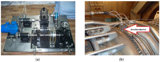
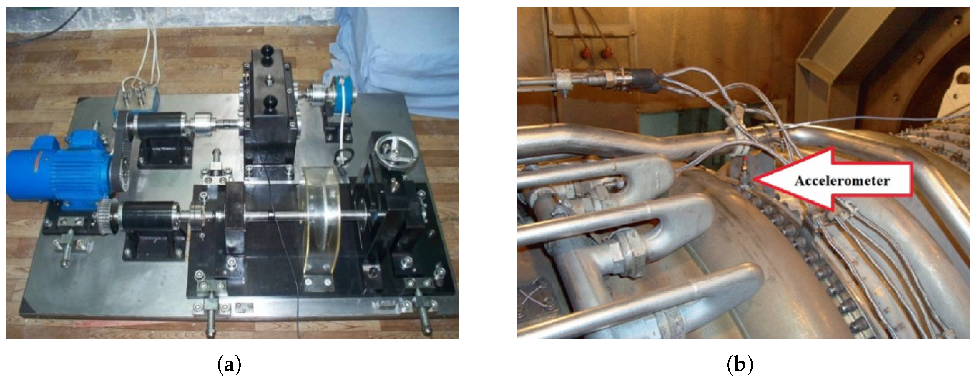
The accelerometer is positioned near the load module, and the applied load is 9500 N. Vibration signals are recorded at a sampling frequency of 50 kHz. The rotational speed is approximately 1500 rpm for all health conditions, and the fault categories are consistent with those used in D1 and D2. Figure 5a depicts the experimental setup for bearing vibration signal acquisition. Figure 5b depicts the aircraft engine bearing test rig used for vibration data collection [38,39].

Figure 5. Vibration data acquisition facilities used for the experimental and practical datasets: (a) experimental setup for bearing vibration signal acquisition; (b) aircraft engine bearing test rig used for vibration data collection.

The practical target-domain dataset D3 contains a total of 2,782,629 vibration sampling points distributed among the 14 fine-grained fault subclasses. Following the same preprocessing procedure adopted throughout this study, each class-specific continuous signal is divided into non-overlapping segments of 550 sampling points, resulting in 5050 target-domain samples. The detailed class distribution is reported in Table 1. Therefore, D3 is moderately imbalanced, with a maximum-to-minimum class size ratio of approximately 3.93:1. Importantly, these target-domain class labels are not used during model training or domain adaptation; they are retained exclusively for final performance evaluation. Reporting the complete class distribution enables the influence of class imbalance on the diagnostic results to be assessed more transparently.

Table 1. Configuration of the two transfer tasks.

Case	Source Domain	Primary State Samples	Sample Length	Target Domain	Target Samples
Case 1	D1	4 × 400	550	D3	5050
Case 2	D2	4 × 260	550	D3	5050

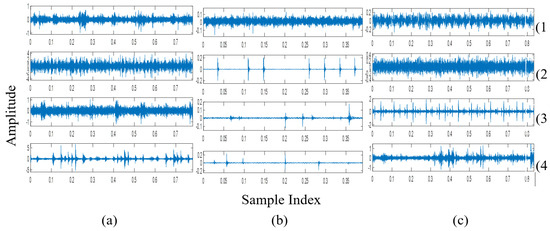
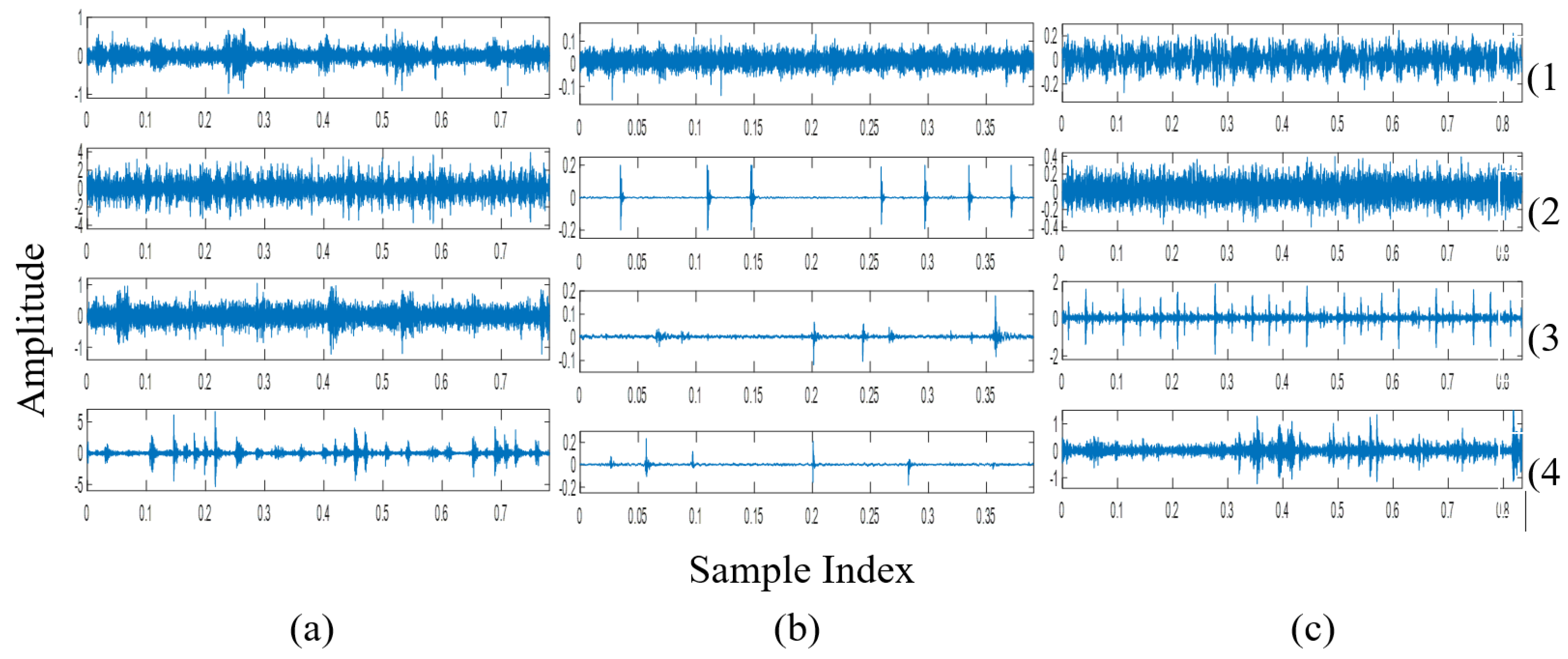
Figure 6 shows representative time-domain vibration waveforms obtained from the three datasets. In this figure, columns (a), (b), and (c) represent the three domains, while rows (1)–(4) correspond to the four primary bearing health states considered in this study: normal (N), ball fault (BA), inner race fault (IR), and outer race fault (OR). Figure 6 presents the signals at the primary health state level for compact visualization, whereas the classification task further distinguishes these categories into the 14 fine-grained subclasses defined above. The plotted signals show clear variations among fault classes as well as noticeable differences among domains. Some waveforms present smooth and regular oscillations, whereas others contain sudden impacts, short-duration transients, and larger amplitude changes. These observations suggest that useful fault information exists in the raw vibration data, but the same fault category may display different signal characteristics when measured under different laboratory or practical conditions. Because D1, D2, and D3 are acquired at different sampling frequencies (48 kHz, 24 kHz, and 50 kHz, respectively), an identical number of signal points corresponds to different physical durations across the three domains. To facilitate direct visual comparison without resampling the original signals, Figure 6 therefore presents the horizontal axis as the sample index. Each waveform contains the same 550 sampling points used as the model input.

Figure 6. Representative time-domain vibration signals from the three domains: (a) D1 laboratory source domain; (b) D2 laboratory source domain; and (c) D3 practical aero-engine target domain. Rows (1)–(4) correspond to the four health states considered in the study.

The significance of this figure is that it visually highlights both class-level differences and domain-level inconsistencies. Variations in waveform structure, impulse strength, and amplitude distribution indicate that samples from the same fault type may not be naturally aligned across domains, while different fault classes may become partially mixed in the original signal space. This challenge motivates the use of the proposed DCL-BiGRU framework. BiGRU is employed to capture temporal dependencies from vibration signals, while deep contrastive learning improves the organization of the feature space by making same-class samples more compact and different-class samples more separable. Therefore, the figure provides a clear visual reason for combining contrastive representation learning with domain adaptation to achieve robust cross-domain aircraft engine fault diagnosis.

The raw vibration recordings from D1, D2, and D3 are processed using the same sample construction procedure. Each continuous vibration sequence is divided into non-overlapping windows containing 550 consecutive sampling points. Each window is regarded as one vibration sample and is represented as a one-dimensional sequence. No change in the temporal sample length is performed before the samples are supplied to the learning models. Therefore, 550 represents the raw input length used consistently for both source- and target-domain samples. The resulting sequences are passed to the feature learning stage, where the BiGRU encoder transforms the 550-point raw sequence into a lower-dimensional latent representation. The projection head subsequently maps this representation into the contrastive feature space, after which perturbation, source classification, and MCD-based target-domain adaptation are performed. The dimensions reported for hidden, projection, and fully connected layers therefore refer to internal learned feature representations rather than to the length of the original vibration signal.

Table 1 summarizes the two cross-domain transfer tasks. In Case 1, D1 is used as the labeled source domain and D3 is used as the practical target domain, forming the D1→D3 transfer task. A total of 400 samples are generated for each of the four health states in D1, resulting in a total of 1600 source-domain samples. In Case 2, D2 is used as the source domain and D3 as the target domain, forming the D2→D3 transfer task. A total of 260 samples are generated for each health state in D2, resulting in 1040 source-domain samples. Here, the notations $4\times 400$ and $4\times 260$ in Table 1 refer to the organization of samples according to the four primary health states. These states collectively contain the 14 fine-grained fault subclasses used as classification labels. Each vibration sample consists of 550 consecutive sampling points. Non-overlapping segmentation is adopted to avoid duplicated signal content between adjacent samples and reduce the possibility of data leakage. During unsupervised domain adaptation, source-domain labels are available for supervised classification and contrastive learning, whereas D3 target-domain labels are withheld from model optimization and used only for final evaluation.

4.2. Comparative Diagnostic Performance

In this section, several well-known transfer learning methods are used as baselines to examine the effectiveness of the proposed framework for label-free cross-domain fault recognition. The compared approaches include Transfer Component Analysis (TCA) [40], Joint Distribution Adaptation (JDA) [41], a multi-layer neural network with MMD regularization (MNN) [42], and a Domain-Adversarial Neural Network (DANN) [43]. For a balanced evaluation, the experimental comparison includes models based on both contrastive representation learning and deep transfer learning. In addition, the planned model is also compared by standalone DCL and BiGRU methods to show why transfer adaptation is necessary when the target-domain data do not contain labels.

The final classification layer contains 14 output neurons corresponding to the 14 fine-grained fault classes. These classes belong to four broader health state categories (N, BA, IR, and OR). Therefore, the four primary health states describe the higher-level fault taxonomy, whereas model training and prediction are performed at the fine-grained 14-class level.

To ensure a fair comparison, a unified input pipeline is adopted for all methods. The continuous vibration recordings from D1, D2, and D3 are divided into the same non-overlapping segments of 550 consecutive sampling points. No method receives separately pre-extracted features. For TCA and JDA, each raw 550-point vibration segment is directly represented as a 550-dimensional vector before kernel-based domain adaptation. For the DCL, BiGRU, MNN, DANN, MCD, CDAN, and proposed DCL-BiGRU framework, the same 550-point segment is supplied to the corresponding model architecture. Consequently, differences in diagnostic performance arise from the feature learning and domain adaptation mechanisms rather than from differences in the original input signal representation.

For consistency, all raw signal-based methods receive vibration segments containing 550 sampling points. The dimensions of the subsequent hidden or feature representations are model-specific architectural parameters and should not be interpreted as different raw signal lengths. For the DCL baseline, the convolutional blocks use 16, 32, and 64 kernels. The learning rates are 0.072 and 0.14 for Case 1 and Case 2, respectively, with 820 and 670 training steps. For the standalone BiGRU model, each direction contains 100 hidden units in Case 1, with a learning rate of 0.013 and 85 training steps. In Case 2, 140 hidden units are used in each direction, with a learning rate of 0.018 and 68 training steps.

For TCA and JDA, the radial basis function kernel is adopted. The adapted feature dimensions of TCA and JDA are set to 70 and 85 in Case 1 and 75 and 85 in Case 2, respectively. The proposed model is also compared with standalone DCL and BiGRU models to demonstrate the importance of explicit domain adaptation when target-domain labels are unavailable. For MNN, the network architecture used in both cases is 500-350-130-65-5. The maximum mean discrepancy regularization term is applied to the representation obtained from the third hidden layer to reduce the distribution difference between the source and target domains.

For the proposed method, the initial BiGRU feature extractor in Case 1 contains 128 hidden units in each direction, uses a learning rate of 0.0014, and is trained for 160 iterations. In Case 2, the corresponding settings are 128 hidden units per direction, a learning rate of 0.0013, and 185 training iterations. The learning rates of the MCD module are 0.00019 for Case 1 and 0.00014 for Case 2, and the corresponding numbers of training iterations are 1500 and 6500. The MCD architecture is identical in both cases, as summarized in Table 2. To reduce randomness and improve the reliability of the comparison, every method is independently repeated five times under its corresponding parameter settings. The detailed experimental results are presented in Table 3.

Table 2. Architecture and internal feature dimensions of the proposed DCL-BiGRU framework.

Layer	Parameters	Output Size
Raw vibration input	Segment length = 550	550 × 1
DCL 1	128-dimensional contrastive feature vector	$128\times 1$
DCL 2	256-dimensional contrastive feature vector	$256\times 1$
Pooling layer	Kernel size = 2; stride = 2	$128\times 1$
Fully connected 0	–	$512\times 1$
Fully connected 1	Weights = $512\times 300$; bias = 300	$300\times 1$
Fully connected 2	Weights = $300\times 100$; bias = 100	$100\times 1$
Fully connected 3	Weights = $100\times 14$; bias = 14	$14\times 1$

Table 3. Cross-domain diagnostic accuracy (%) of the compared methods.

Method	Input	Case 1 Accuracy (%)	Case 2 Accuracy (%)	Average (%)
DCL	Raw vibration signals	$82.16\pm 0.80$	$77.68\pm 1.10$	79.92
BiGRU	Raw vibration signals	$81.38\pm 0.92$	$78.89\pm 2.05$	80.13
TCA	Raw vibration signals	$73.57\pm 1.53$	$73.14\pm 1.38$	74.52
JDA	Raw vibration signals	$74.65\pm 1.13$	$74.39\pm 1.20$	71.60
MNN	Raw vibration signals	$78.91\pm 1.81$	$74.69\pm 2.22$	76.80
DANN	Raw vibration signals	$80.98\pm 2.40$	$77.67\pm 1.98$	79.32
MCD	Raw vibration signals	$83.98\pm 1.75$	$84.28\pm 1.82$	84.13
CDAN	Raw vibration signals	$82.87\pm 1.30$	$81.96\pm 1.36$	82.41
Proposed method	Raw vibration signals	$95.62\pm 1.14$	$92.48\pm 1.17$	94.05

Note: Results are reported as mean accuracy (%) ± standard deviation over five independent runs.

Table 3 presents the cross-domain diagnostic accuracies of all compared methods. The proposed DCL-BiGRU achieves accuracies of 95.62% ± 1.14% in Case 1 and 92.48% ± 1.17% in Case 2, resulting in an average accuracy of 94.05%. In Case 1, DCL is the strongest baseline with an accuracy of 82.16%; therefore, the proposed method provides an improvement of 13.46 percentage points. In Case 2, BiGRU obtains the highest baseline accuracy of 78.89%, whereas the proposed method improves this result by 13.59 percentage points. In terms of average performance, the best baseline is BiGRU at 80.13%, while DCL-BiGRU achieves 94.05%, corresponding to an improvement of 13.92 percentage points. These quantitative results demonstrate that combining bidirectional temporal feature extraction, contrastive representation learning, perturbation-based robustness, and boundary-aware domain adaptation provides substantially better cross-domain fault diagnosis performance than the individual feature learning and domain adaptation approaches.

An additional observation from Table 3 is that the relative performance of standalone DCL and BiGRU changes between the two transfer tasks. In Case 1 (D1→D3), DCL achieves 82.16%, slightly exceeding the 81.38% obtained by BiGRU, whereas, in Case 2 (D2→D3), BiGRU achieves 78.89% compared with 77.68% for DCL. This suggests that the effectiveness of discriminative contrastive representation learning and temporal sequence modeling depends on the characteristics of the source–target domain shift. D1 is acquired at 48 kHz and 1797 rpm, which is relatively close to the D3 acquisition conditions of 50 kHz and approximately 1500 rpm. In contrast, D2 is acquired at 24 kHz and 700 rpm, resulting in a substantially larger mismatch with D3 in both sampling frequency and rotational speed. Such differences can modify the temporal and frequency characteristics of bearing vibration signals and may explain why all evaluated methods show lower performance in Case 2. The proposed framework remains comparatively robust under both conditions because BiGRU captures temporal dependencies, contrastive learning preserves fault class structure, and MCD-based adaptation adjusts target representations according to classifier decision boundaries. Perturbation further improves robustness to feature variations. Therefore, the proposed approach maintains high diagnostic accuracy even for the more challenging D2→D3 transfer task.

To further verify the contribution of each module in the proposed framework, an ablation study is conducted by gradually removing or adding DCL, BiGRU, MCD, and the perturbation strategy. The results are summarized in Table 4.

Table 4. Ablation study of key components in the proposed DCL-BiGRU framework.

Model Variant	Case 1 Accuracy (%)	Case 2 Accuracy (%)	Average Accuracy (%)
BiGRU only	$81.38\pm 0.92$	$78.89\pm 2.05$	80.13
DCL + BiGRU	$86.30\pm 1.01$	$87.69\pm 1.50$	86.99
BiGRU + MCD	$84.16\pm 1.82$	$85.86\pm 1.73$	85.01
DCL + BiGRU + MCD	$88.95\pm 2.10$	$91.16\pm 2.08$	89.06
BiGRU + MCD + Perturbation	$87.96\pm 1.75$	$91.01\pm 1.78$	88.49
DCL + BiGRU + MCD + Perturbation	$95.62\pm 1.14$	$92.48\pm 1.17$	94.05

Note: Results are reported as mean accuracy (%) ± standard deviation over five independent runs using the same experimental protocol for all ablation configurations.

4.3. Visualization of Learned Fault Features

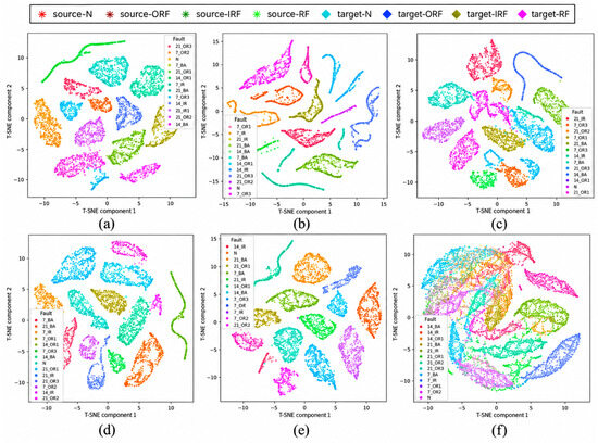
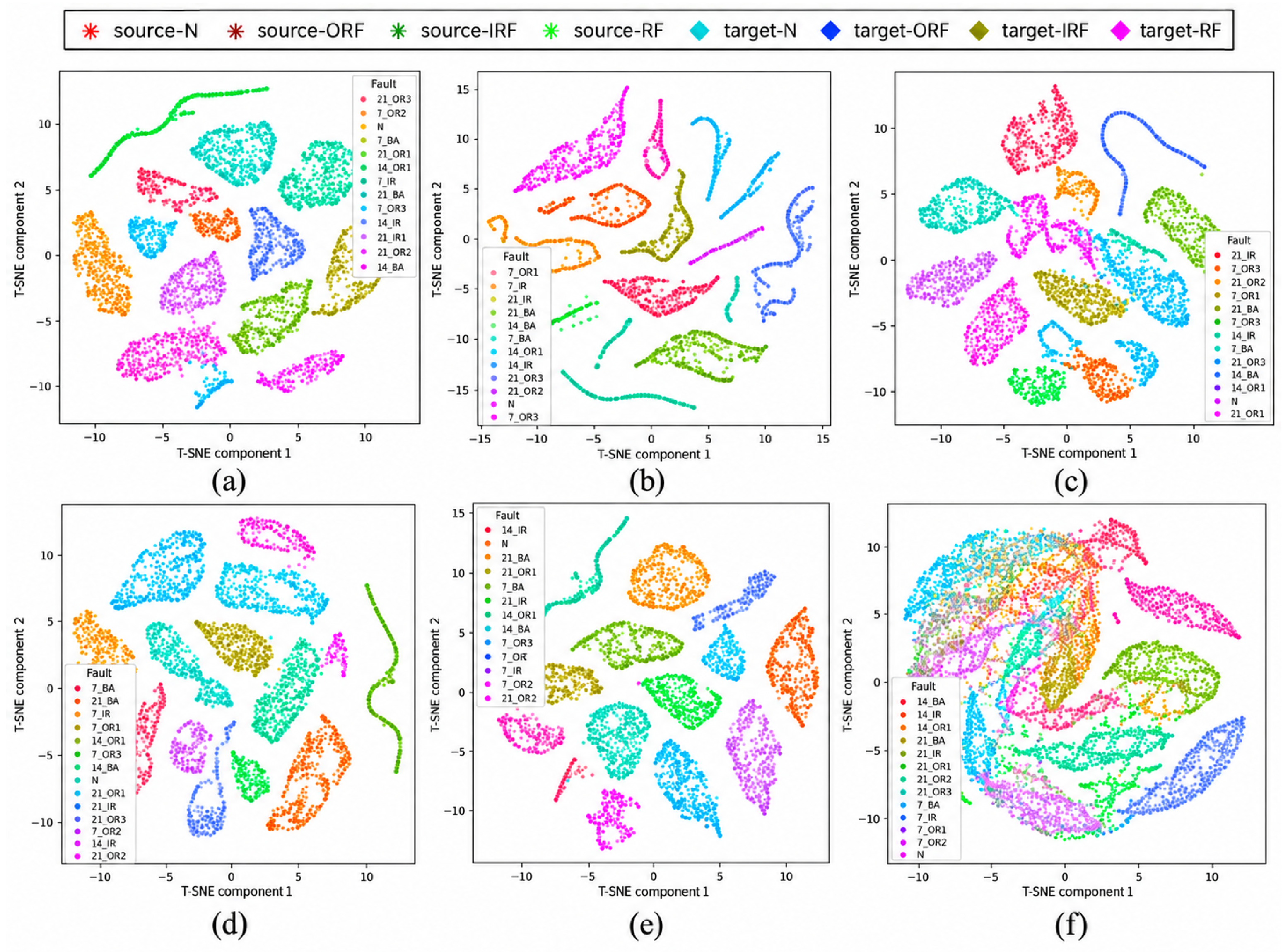
To provide an intuitive interpretation of the learned feature representations, t-distributed stochastic neighbor embedding (t-SNE) [44] is employed to project the high-dimensional features into a two-dimensional space. This visualization helps illustrate how the proposed transfer learning framework progressively improves feature distribution across domains. The corresponding results for the two transfer cases are shown in Figure 7.

Figure 7. t-SNE visualization of the feature distributions produced by the proposed DCL-BiGRU framework for two cross-domain transfer cases. (a) Raw/input feature space for Case 1 (D1→D3); (b) BiGRU-extracted feature space for Case 1; (c) adapted feature space after MCD optimization for Case 1; (d) raw/input feature space for Case 2 (D2→D3); (e) BiGRU-extracted feature space for Case 2; and (f) MCD-adapted feature space for Case 2. Different colors denote the fault categories, while the source- and target-domain samples are distinguished according to the markers shown in the legend.

For clarity of cross-domain visualization, Figure 7 groups the fine-grained subclasses according to the four primary health states (N, BA, IR, and OR), whereas Figure 8 and Figure 9 retain the 14 individual subclass labels for fine-grained feature and classification analysis. Specifically, for Case 1, the visualization results are shown in Figure 7a–c, while Case 2 is represented by Figure 7d–f. The first visualization in each case corresponds to the raw signal space, the second to the BiGRU-extracted feature space, and the third to the adapted feature space after MCD optimization. These results demonstrate that the proposed method gradually improves feature alignment between domains and forms more compact class-wise clusters.

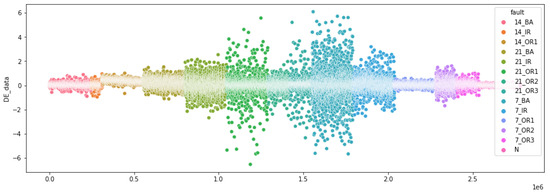
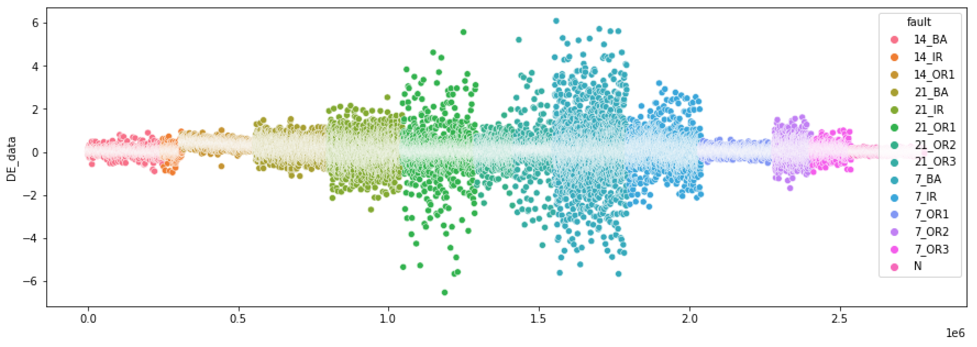
Figure 8. Deep embedding (DE) visualization of the 14 fine-grained fault subclasses.

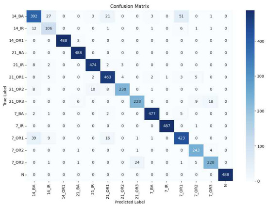
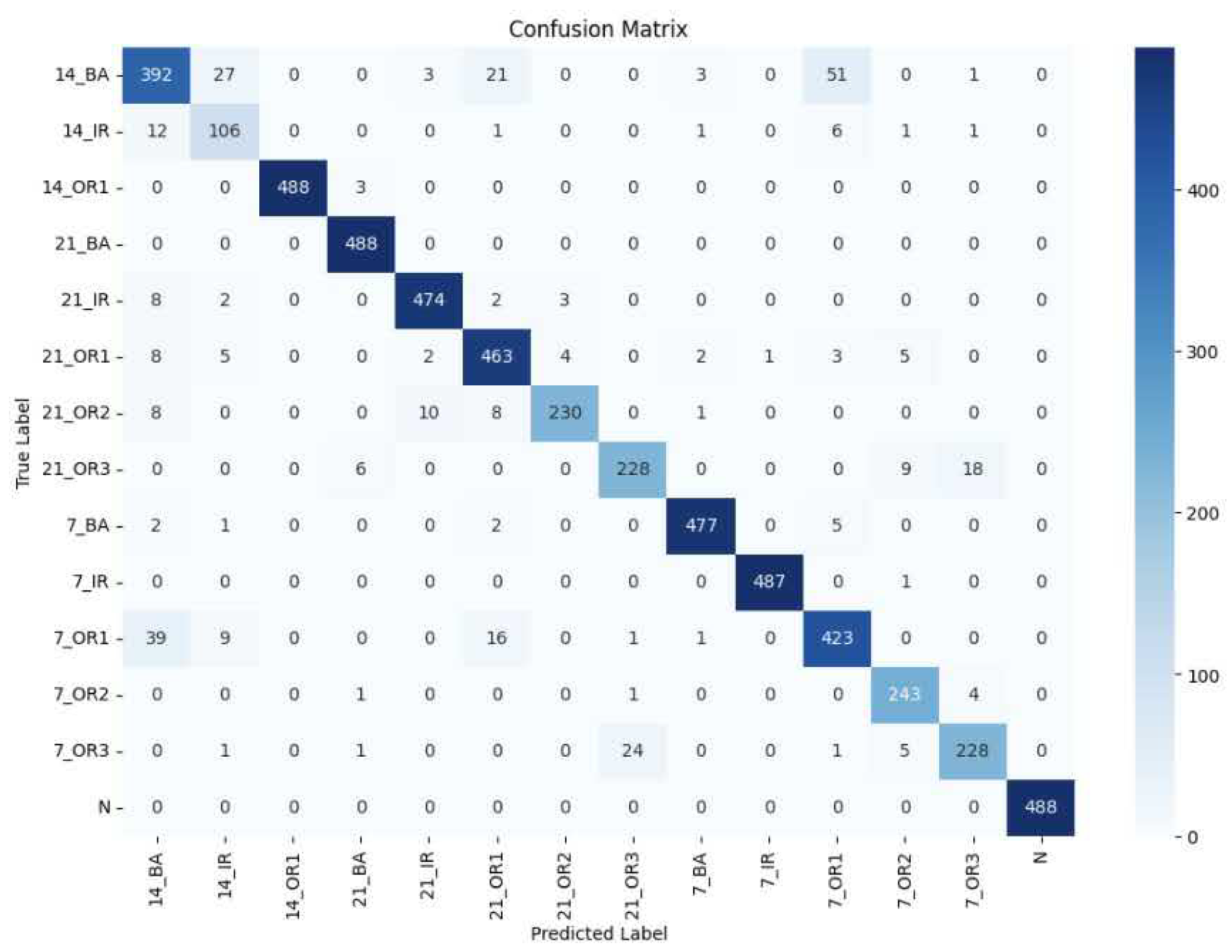
Figure 9. Confusion matrix of the proposed DCL-BiGRU model for cross-domain aero-engine fault detection.

4.4. Deep Embedding Analysis

Figure 8 presents the deep embedding (DE) visualization of the 14 fine-grained fault subclasses belonging to the four primary health states. The high-dimensional learned representations are projected into two dimensions, with each point representing a sample and colored according to its corresponding fine-grained fault label. The resulting clusters show clear and distinct groupings for most fault categories, such as 14_BA, 14_OR1, 21_BA, 7_IR, and N, indicating that the deep model has successfully learned meaningful representations that differentiate these classes. However, some clusters, particularly 21_OR2, 21_OR3, and 7_OR1, appear closer together and show slight overlap, suggesting that these faults may share subtle feature similarities or that their boundaries in the learned feature space are not entirely separable. The symmetry around the central axis reflects structural similarities and balanced distributions in the underlying signal features. Overall, the DE visualization supports the model’s ability to distinguish most fault types effectively, while also highlighting specific classes that may benefit from additional refinement in feature learning or class separation.

4.5. Fault Class Confusion Analysis

Figure 9 presents the fine-grained classification performance of the proposed DCL-BiGRU model over the 14 subclasses associated with the four primary health states. Each row represents the actual fine-grained fault class, while each column represents the corresponding predicted class. The strong presence of high values along the diagonal (dark blue cells) signifies that the majority of predictions are correct for most classes. For instance, the model accurately classifies almost all samples from classes like 14_OR1 (488), 21_BA (488), 7_IR (487), and N (488), indicating excellent performance in these categories. However, a few areas show noticeable misclassification. The class 14_BA, while mostly correctly predicted (392), has 51 samples misclassified as “N” and 27 as 14_IR, suggesting some ambiguity between these classes or overlap in feature space. Similarly, 21_OR2 and 21_OR3 show lower correct predictions (230 and 228, respectively), and some of their instances are confused with each other and with class N or 21_IR. Additionally, 7_OR1 has 423 correct predictions but is also frequently misclassified as 14_OR1 (39 instances) and 21_OR1 (16 instances), which might indicate that these classes share similar features or patterns. A few minor misclassifications are scattered across the matrix, but they remain relatively low in frequency. Overall, the model demonstrates strong classification ability with high accuracy across most classes.

To provide a more comprehensive evaluation of the fine-grained classification task, precision, recall, and F1-score are further calculated for each of the 14 diagnostic subclasses. The corresponding results are summarized in Table 5. In addition to class-wise performance, macro-averaged metrics are calculated to give equal importance to every class irrespective of its sample frequency. The model achieves a Macro-Precision of 92.34%, Macro-Recall of 92.72%, and Macro-F1 of 92.47%. The class-wise results indicate that most fault categories are recognized reliably, while some classes remain comparatively more challenging because of similarity in their vibration characteristics. These observations are consistent with the confusion patterns shown in Figure 9.

Table 5. Per-class performance of the proposed DCL-BiGRU model on the 14-class fine-grained diagnosis task.

Class	Precision (%)	Recall (%)	F1-Score (%)
14_BA	83.58	78.71	81.08
14_IR	70.20	82.81	75.99
14_OR1	100.00	99.39	99.69
21_BA	97.80	100.00	98.89
21_IR	96.93	96.93	96.93
21_OR1	90.25	93.91	92.05
21_OR2	97.05	89.49	93.12
21_OR3	89.76	87.36	88.54
7_BA	98.35	97.95	98.15
7_IR	99.80	99.80	99.80

4.6. Negative Transfer, Hyperparameter Sensitivity, and Convergence Analysis

To further evaluate the robustness of the coupled optimization procedure, additional analyses are conducted to investigate the possibility of negative transfer, the influence of the loss-weighting coefficients ${\lambda }_c$ and $\beta$, and the convergence behavior of the proposed DCL-BiGRU framework. Because the source-supervised contrastive objective and target-domain discrepancy objective affect the shared representation in different ways, an inappropriate balance between these objectives may reduce cross-domain transferability.

4.6.1. Hyperparameter Sensitivity Analysis

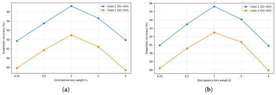
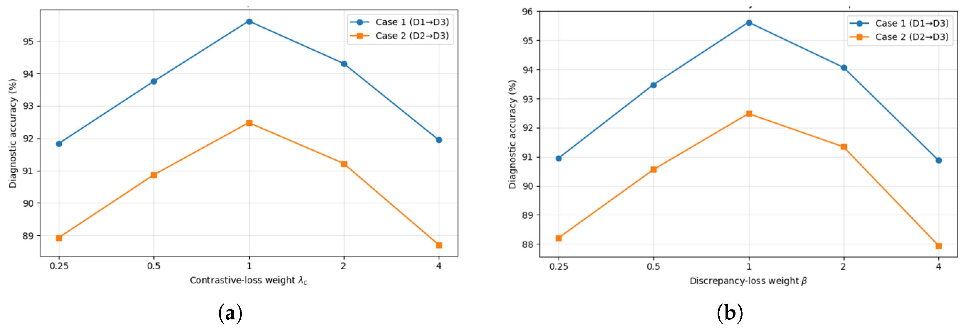
The sensitivity of the model to the contrastive loss coefficient ${\lambda }_c$ and discrepancy loss coefficient $\beta$ is analyzed. Figure 10 presents the effect of ${\lambda }_c$ and $\beta$ on diagnostic accuracy for both transfer tasks. Moderate coefficient values provide the best balance between source-domain class discrimination and target-domain adaptation. When ${\lambda }_c$ is small, the contrastive constraint becomes insufficient to maintain compact intra-class and separated inter-class representations. In contrast, a large ${\lambda }_c$ overemphasizes source-domain class structure and may reduce transferability to the target domain. Similarly, a small $\beta$ leads to insufficient target-domain adaptation, whereas a large $\beta$ may place excessive emphasis on classifier discrepancy and cause uncertain target features to move too strongly toward source-supported regions.

Figure 10. Sensitivity of the proposed DCL-BiGRU model to (a) the contrastive loss coefficient ${\lambda }_c$ and (b) the discrepancy loss coefficient $\beta$ for Case 1 and Case 2.

The best performance is obtained around the selected operating point, where the model achieves 95.62% accuracy in Case 1 and 92.48% in Case 2. The relatively gradual variation around this region indicates that the framework is not excessively sensitive to moderate changes in either coefficient.

4.6.2. Convergence and Training Stability

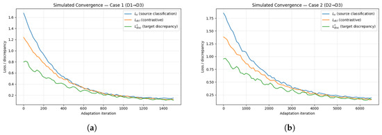
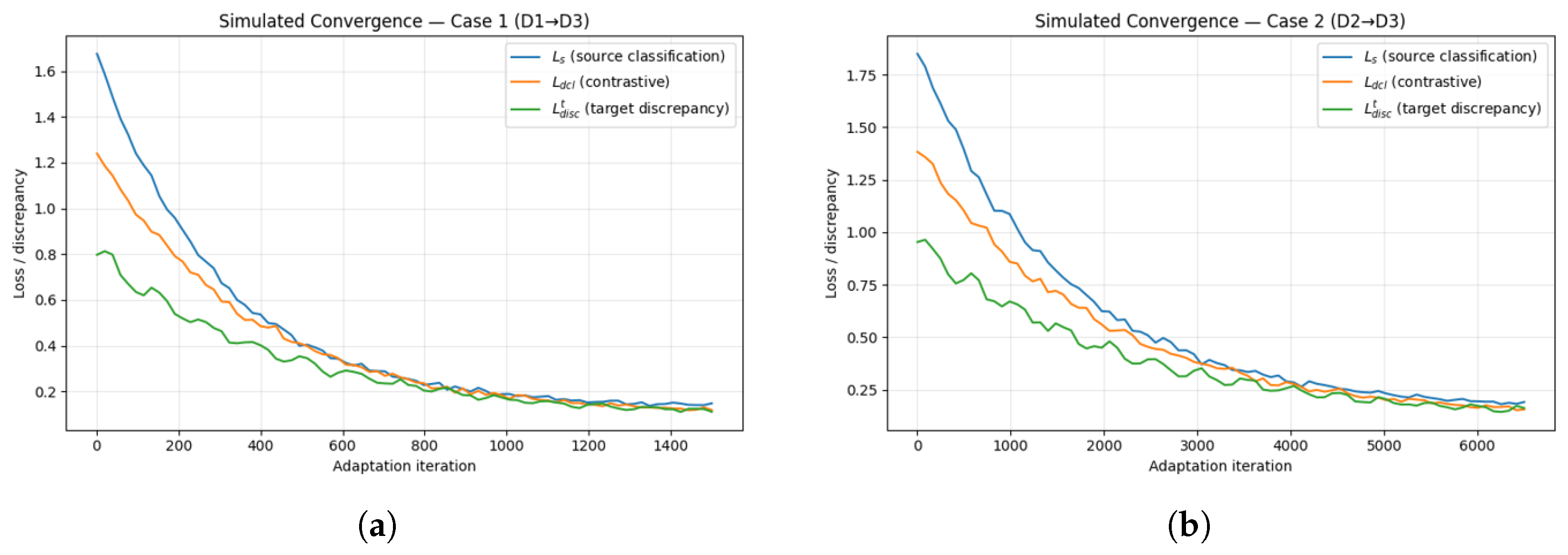
The convergence behavior of the proposed alternating optimization procedure is also examined for both transfer tasks. Figure 11 shows the evolution of the source classification loss Ls, contrastive loss $L_{dcl}$, and target-domain classifier discrepancy $L_{disc}^t$ during adaptation. For Case 1, the analysis covers 1500 adaptation iterations, whereas Case 2 is evaluated over 6500 iterations, consistent with the training settings used in the proposed model. The source classification and contrastive losses progressively decrease and approach stable regions during training. The target-domain discrepancy also decreases overall while exhibiting small local fluctuations due to the alternating discrepancy maximization and discrepancy minimization mechanism of MCD. These fluctuations are expected because the classifiers first increase their disagreement to identify uncertain target samples, after which the feature extractor is optimized to reduce that disagreement. Importantly, the loss trajectories remain bounded and do not exhibit persistent divergence, supporting the numerical stability of the coupled optimization procedure.

Figure 11. Convergence behavior of the proposed DCL-BiGRU framework: (a) Case 1 (D1→D3) and (b) Case 2.

5. Conclusions

This study proposed a perturbation-enhanced DCL-BiGRU transfer learning framework for cross-domain aero-engine fault detection. The method combines BiGRU-based temporal feature extraction with an MCD adversarial adaptation mechanism to improve knowledge transfer from labeled experimental data to unlabeled practical engine data. Different from conventional alignment methods, the proposed framework contemplates the position of target samples relative to class decision boundaries, enabling more reliable classification under domain shift. The use of deep contrastive learning further improves feature compactness within the same fault class and separation between different fault categories.

Experiments on three aircraft engine datasets under two transfer scenarios verified the effectiveness of the proposed model, which achieved a mean accuracy of 94.05%, demonstrating stronger diagnostic performance than the TCA, JDA, DANN, MNN, and BiGRU-only baseline. Visualization and classification analyses confirmed that the learned feature space is better aligned across domains and more effective for distinguishing fault categories. The key contributions include bidirectional temporal feature learning, MCD-based boundary-aware adaptation, and validation on both experimental and practical datasets. Future work will consider multi-sensor data fusion, self-supervised learning, and real-time deployment for online aircraft engine fault detection.

References

- Szrama, S.; Lodygowski, T. Aircraft Engine Remaining Useful Life Prediction using neural networks and real-life engine operational data. Adv. Eng. Softw. 2024, 192, 103645. [Google Scholar] [CrossRef] [Scilit]
- Zhu, Z.; Lei, Y.; Qi, G.; Chai, Y.; Mazur, N.; An, Y.; Huang, X. A review of the application of deep learning in intelligent fault diagnosis of rotating machinery. Measurement 2023, 206, 112346. [Google Scholar] [CrossRef] [Scilit]
- Vashishtha, G.; Chauhan, S.; Sehri, M.; Zimroz, R.; Dumond, P.; Kumar, R.; Gupta, M.K. A roadmap to fault diagnosis of industrial machines via machine learning: A brief review. Measurement 2025, 242, 116216. [Google Scholar] [CrossRef] [Scilit]
- Jin, Y.; Hou, L.; Chen, Y. A Time Series Transformer based method for the rotating machinery fault diagnosis. Neurocomputing 2022, 494, 379–395. [Google Scholar] [CrossRef] [Scilit]
- Tama, B.A.; Vania, M.; Lee, S.; Lim, S. Recent advances in the application of deep learning for fault diagnosis of rotating machinery using vibration signals. Artif. Intell. Rev. 2023, 56, 4667–4709. [Google Scholar] [CrossRef] [Scilit]
- Xiao, X.; Li, C.; Huang, J.; Yu, T. Rotating machinery fault diagnosis based on one-dimensional convolutional neural network and modified multi-scale graph convolutional network under limited labeled data. Eng. Appl. Artif. Intell. 2024, 137, 109129. [Google Scholar] [CrossRef] [Scilit]
- Wu, Y.; Ma, X. A hybrid LSTM-KLD approach to condition monitoring of operational wind turbines. Renew. Energy 2022, 181, 554–566. [Google Scholar] [CrossRef] [Scilit]
- Gao, Y.; Kim, C.H.; Kim, J.-M. A novel hybrid deep learning method for fault diagnosis of rotating machinery based on extended WDCNN and long short-term memory. Sensors 2021, 21, 6614. [Google Scholar] [CrossRef] [Scilit] [PubMed]
- Wu, J.; Kong, L.; Kang, S.; Zuo, H.; Yang, Y.; Cheng, Z. Aircraft Engine Fault Diagnosis Model Based on 1DCNN-BiLSTM with CBAM. Sensors 2024, 24, 780. [Google Scholar] [CrossRef] [Scilit] [PubMed]
- Li, B.; Zhao, Y.P.; Chen, Y.B. Unilateral alignment transfer neural network for fault diagnosis of aircraft engine. Aerosp. Sci. Technol. 2021, 118, 107031. [Google Scholar] [CrossRef] [Scilit]
- Shao, H.; Cheng, J.; Hongkai, J.; Yu, Y.; Zhantao, W. Enhanced deep gated recurrent unit and complex wavelet packet energy moment entropy for early fault prognosis of bearing. Knowl.-Based Syst. 2019, 188, 105022. [Google Scholar] [CrossRef] [Scilit]
- Zhao, R.; Wang, D.; Yan, R.; Mao, K. Machine health monitoring using local feature-based gated recurrent unit networks. IEEE Trans. Ind. Electron. 2018, 65, 1539–1548. [Google Scholar] [CrossRef] [Scilit]
- ElDali, M.; Kumar, K.D. Fault diagnosis and prognosis of aerospace systems using growing recurrent neural networks and LSTM. In Proceedings of the 2021 IEEE Aerospace Conference (50100), Big Sky, MT, USA, 6–13 March 2021. [Google Scholar]
- Tian, H.; Fan, H.; Feng, M.; Cao, R.; Li, D. Fault Diagnosis of Rolling Bearing Based on HPSO Algorithm Optimized CNN-LSTM Neural Network. Sensors 2023, 23, 6508. [Google Scholar] [CrossRef] [Scilit] [PubMed]
- Zhao, K.; Jiang, H.K.; Li, X.; Wang, R. An optimal deep sparse autoencoder with gated recurrent unit for rolling bearing fault diagnosis. Meas. Sci. Technol. 2020, 31, 015005. [Google Scholar] [CrossRef] [Scilit]
- Misbah, I.; Lee, C.K.M.; Keung, K.L. Fault diagnosis in rotating machines based on transfer learning: Literature review. Knowl.-Based Syst. 2024, 283, 111158. [Google Scholar] [CrossRef] [Scilit]
- Tang, S.; Ma, J.; Yan, Z.; Zhu, Y.; Khoo, B.C. Deep transfer learning strategy in intelligent fault diagnosis of rotating machinery. Eng. Appl. Artif. Intell. 2024, 134, 108678. [Google Scholar] [CrossRef] [Scilit]
- Li, W.; Huang, R.; Li, J.; Liao, Y.; Chen, Z.; He, G.; Yan, R.; Gryllias, K. A perspective survey on deep transfer learning for fault diagnosis in industrial scenarios: Theories, applications and challenges. Mech. Syst. Signal Process. 2022, 167, 108487. [Google Scholar] [CrossRef] [Scilit]
- Yin, K.; Shen, Y.; Chen, Y.; Zhang, H. Multi-Source Information Fusion Diagnosis Method for Aero Engine. Appl. Sci. 2025, 15, 5083. [Google Scholar] [CrossRef] [Scilit]
- Zhang, H.; Chen, X.; Zhang, X.; Ye, B.; Wang, X. Aero-engine bearing fault detection: A clustering low-rank approach. Mech. Syst. Signal Process. 2020, 138, 106529. [Google Scholar] [CrossRef] [Scilit]
- Zhuang, F.; Qi, Z.; Duan, K.; Xi, D.; Zhu, Y.; Zhu, H.; Xiong, H.; He, Q. A Comprehensive Survey on Transfer Learning. Proc. IEEE 2020, 109, 43–76. [Google Scholar] [CrossRef] [Scilit]
- Kumar, P.; Singh, S.; Song, D.Y. Investigation of Transfer Learning Method for Motor Fault Detection. Machines 2025, 13, 329. [Google Scholar] [CrossRef] [Scilit]
- Qian, Q.; Qin, Y.; Luo, J.; Wang, Y.; Wu, F. Deep discriminative transfer learning network for cross-machine fault diagnosis. Mech. Syst. Signal Process. 2022, 186, 109884. [Google Scholar] [CrossRef] [Scilit]
- Bao, Z.; Liu, C.; Yang, H.; Zhang, J.; Li, Y. From theory to industry: A survey of deep learning-enabled bearing fault diagnosis in complex environments. Eng. Appl. Artif. Intell. 2026, 163, 113068. [Google Scholar] [CrossRef] [Scilit]
- Wu, H.; Li, J.; Zhang, Q.; Tao, J.; Meng, Z. Intelligent fault diagnosis of rolling bearings under varying operating conditions based on domain-adversarial neural network and attention mechanism. Isa Trans. 2022, 130, 477–489. [Google Scholar] [CrossRef] [Scilit] [PubMed]
- Mao, W.; Liu, Y.; Ding, L.; Safian, A.; Liang, X. A Deep Domain-Adversarial Transfer Fault Diagnosis Method for Rolling Bearing Based on Ensemble Empirical Mode Decomposition. J. Sens. 2022, 2022, 8959185. [Google Scholar] [CrossRef] [Scilit]
- Zhang, S.; Su, L.; Gu, J.; Li, K.; Zhou, L.; Pecht, M.; Li, J. Rotating machinery fault detection and diagnosis based on deep domain adaptation: A survey. Chin. J. Aeronaut. 2023, 36, 45–74. [Google Scholar] [CrossRef] [Scilit]
- Jia, S.; Deng, Y.; Lv, J.; Du, S.; Xie, Z. Joint distribution adaptation with diverse feature aggregation: A new transfer learning framework for bearing diagnosis across different machines. Measurement 2022, 187, 110332. [Google Scholar] [CrossRef] [Scilit]
- Xiao, Y.; Wang, J.; He, Z.; Zhou, H.; Zhu, H. Deep transfer learning with metric structure for fault diagnosis. Knowl.-Based Syst. 2022, 256, 109826. [Google Scholar] [CrossRef] [Scilit]
- Shao, J.; Huang, Z.; Zhu, Y.; Zhu, J.; Fang, D. Rotating machinery fault diagnosis by deep adversarial transfer learning based on subdomain adaptation. Adv. Mech. Eng. 2021, 13, 16878140211040226. [Google Scholar] [CrossRef] [Scilit]
- Choi, S.H.; Park, J.K.; An, D.; Kim, C.H.; Park, G.; Lee, I.; Lee, S. Fault Diagnosis Method for Human Coexistence Robots Based on Convolutional Neural Networks Using Time-Series Data Generation and Image Encoding. Sensors 2023, 23, 9753. [Google Scholar] [CrossRef] [Scilit] [PubMed]
- Liu, Z.H.; Lu, B.L.; Wei, H.L.; Chen, L.; Li, X.H.; Rätsch, M. Deep adversarial domain adaptation model for bearing fault diagnosis. IEEE Trans. Syst. Man Cybern. Syst. 2021, 51, 4217–4226. [Google Scholar] [CrossRef] [Scilit]
- Zhao, M.; Zhong, S.; Fu, X.; Tang, B.; Pecht, M. Deep Residual Shrinkage Networks for Fault Diagnosis. IEEE Trans. Ind. Inform. 2019, 16, 4681–4690. [Google Scholar] [CrossRef] [Scilit]
- Wang, C.; Wu, S.; Shao, X. Unsupervised domain adaptive bearing fault diagnosis based on maximum domain discrepancy. Eurasip J. Adv. Signal Process. 2024, 11, 2024. [Google Scholar] [CrossRef] [Scilit]
- Case Western Reserve University Bearing Data Center Website. Available online: https://engineering.case.edu/bearingdatacenter (accessed on 12 May 2026).
- Hu, K.; Cheng, Y.; Wu, J.; Zhu, H. Cross-domain intelligent diagnostics for rotating machinery using domain adaptive and adversarial networks. J. Ind. Inf. Integr. 2024, 42, 100722. [Google Scholar] [CrossRef] [Scilit]
- Li, D.; Ma, M. A Bearing Fault Diagnosis Method Based on Improved Transfer Component Analysis and Deep Belief Network. Appl. Sci. 2024, 14, 1973. [Google Scholar] [CrossRef] [Scilit]
- Ahmad, S.H.; Jiang, H.K.; Rabiu, B.I.; Hassan, S.M.H.U. Fault diagnosis of aircraft engine using an ANN-BiGRU based on perturbation strategy. Aerosp. Sci. Technol. 2026, 168, 11047. [Google Scholar] [CrossRef] [Scilit]
- Ahmad, S.H.; Jiang, H.K.; Hassan, S.M.H.U.; Rabiu, B.I. Aircraft engine fault diagnosis using a Mamba-BiGRU model with perturbation strategy. Aerosp. Sci. Technol. 2026, 175, 111988. [Google Scholar] [CrossRef] [Scilit]
- Wang, L.; Li, Y.; Zhang, C.; Sangalang, R.G. Research on bearing fault feature transfer diagnosis based on balanced distribution adaptation under feature fusion. Adv. Mech. Eng. 2025, 17, 16878132251348366. [Google Scholar] [CrossRef] [Scilit]
- Jiang, K.; Cai, Y.; Han, D.; Su, Y.; Li, Z.; Wang, Q.; Feng, G. MDEA-Net: Multisource disentangled expert adaptation network for cross-domain bearing fault diagnosis. Struct. Health Monit. 2026, 14759217261421679. [Google Scholar] [CrossRef] [Scilit]
- Pan, X.; Chen, H.; Wang, W.; Su, X. Adversarial domain adaptation based on contrastive learning for bearings fault diagnosis. Simul. Model. Pract. Theory 2025, 139, 103058. [Google Scholar] [CrossRef] [Scilit]
- Liu, X.M.; Zhang, R.M.; Li, J.P.; Xu, Y.F.; Li, K. A motor bearing fault diagnosis model based on multi-adversarial domain adaptation. Sci. Rep. 2024, 14, 29078. [Google Scholar] [CrossRef] [Scilit] [PubMed]
- Poličar, P.G.; Stražar, M.; Zupan, B. openTSNE: A Modular Python Library for t-SNE Dimensionality Reduction and Embedding. J. Stat. Softw. 2024, 109, 1–30. [Google Scholar] [CrossRef] [Scilit]
Disclaimer/Publisher’s Note: The statements, opinions and data contained in all publications are solely those of the individual author(s) and contributor(s) and not of MDPI and/or the editor(s). MDPI and/or the editor(s) disclaim responsibility for any injury to people or property resulting from any ideas, methods, instructions or products referred to in the content. |
© 2026 by the authors. Licensee MDPI, Basel, Switzerland. This article is an open access article distributed under the terms and conditions of the Creative Commons Attribution (CC BY) license.