


Abstract
This study proposes a genetic algorithm-enhanced dhole optimization algorithm coupled with a long short-term memory network (GA-DOA-LSTM) for dynamic identification of a high bypass ratio separate-flow turbofan engine during acceleration. A component-level JT9D model was implemented in T-MATS, and a dataset was generated at 54 flight operating points under step, ramp, and parabolic throttle excitations. Low- and high-pressure spool speeds, high-pressure compressor outlet total pressure, combustor exit temperature, and fuel flow were used as inputs, while low-pressure turbine exit temperature (T5) and thrust were predicted. GA-DOA combines dual-population coevolution, a global optimum pool, periodic elite exchange, greedy selection, and a final DOA refinement to jointly optimize the LSTM architecture and output loss weights. Compared with LSTM, PSO-LSTM, SSA-LSTM, DOA-LSTM, and GA-LSTM, the proposed model achieved RMSE, MAE, and MAPE values of 1.6121 K, 1.0136 K, and 0.1512% for T5 and 2430.10 N, 1832.24 N, and 1.2576% for thrust, respectively. The model maintained consistent transient tracking under different altitudes, Mach numbers, and throttle profiles, demonstrating its potential for aero-engine performance assessment, health monitoring, and control-oriented modeling. The main limitation is that the present validation remains simulation-based and engine-specific; experimental and cross-engine validation will therefore be required before practical deployment.
1. Introduction
High bypass ratio separate-flow turbofan engines offer high propulsive efficiency, low specific fuel consumption, and high thrust, and are widely used in large commercial aircraft and long-range transport platforms [1]. Compared with engines of low or medium bypass ratio, they have a larger bypass duct gas volume and a higher overall pressure ratio, resulting in stronger aerodynamic–thermodynamic coupling between the core and bypass streams. Fan inertia, off-design matching of multistage compressors, and transient spool speed mismatch make the transition process strongly nonlinear, multivariable, coupled, and time varying [2]. During acceleration from idle to maximum power, fuel flow, spool speeds, and temperatures evolve rapidly along nonlinear trajectories, which are difficult to represent accurately with conventional linearized models [3]. An accurate dynamic model is therefore essential for control system design and performance assessment.
First-principles models require complex component-level aerodynamic and thermodynamic equations and are expensive to construct and solve, whereas excessive simplification may compromise transient prediction accuracy. Data-driven approaches can learn nonlinear input–output mappings directly from operating data and have therefore been increasingly applied to aero-engine performance prediction because of their flexibility and relatively low computational cost [4].
System identification and machine learning methods have recently been applied to aero-engine dynamic modeling. Liao et al. investigated stream fine-tuning for on-board aero-engine gas path diagnosis under continuing domain shifts and validated the approach using simulation and actual engine data [5]. Wang et al. introduced a NARMAX structure and the Akaike information criterion into a local linear model tree, improving the nonlinear identification of aero-engine transients [6]. Asgari and Ory developed a recurrent neural network model for a single-shaft gas turbine and demonstrated the ability of neural networks to capture nonlinear system dynamics [7]. Vu et al. estimated engine performance from multi-point and multi-time operating data under limited sensing [8]. Chen et al. optimized a NARX network with the sparrow search algorithm (SSA) for dynamic parameter identification [9].
Recent studies further demonstrate the rapid development of data-driven aero-engine performance modeling. Cui et al. developed an autoregressive process neural network model for gas path parameter prediction [10], while Wang et al. combined a sliding window LSTM with a denoising autoencoder for gas path monitoring under noisy conditions [11]. Liu et al. applied LSTM to single- and multi-step gas path parameter trend prediction [12], and Meng et al. proposed a temporal convolutional network for thrust estimation with embedded verification [13]. Physics-guided deep learning has also been investigated for exhaust gas temperature prediction and health management [14], and machine learning has been used to adapt turbofan performance models to measured operating data [15]. More recently, GA-LSTM has been applied to gas turbine performance degradation prediction using limited experimental data [16], confirming the value of automatic hyperparameter tuning but also showing that combining GA with LSTM alone is not, by itself, a sufficient methodological distinction.
Long short-term memory (LSTM) networks use gated memory cells to mitigate vanishing gradients and learn long-term dependencies in sequential data [17]. Lin et al. developed LSTM-based gas path performance prognostic models that account for time series characteristics, operating conditions, and engine-to-engine differences using real-life aero-engine data [18], and Ma et al. proposed a feature attention-enhanced LSTM with an encoder–decoder structure to reduce long-horizon prediction errors [19]. However, the architecture and training hyperparameters of these models are commonly selected manually or initialized randomly, which may impair accuracy and stability. A single swarm optimizer may also converge prematurely or search inefficiently when used to tune an LSTM.
Against this background, the contribution of the present study is not merely the application of another metaheuristic optimizer to an LSTM. Instead, a cooperative GA-DOA framework is constructed for multi-output dynamic identification of a high bypass ratio turbofan engine. GA maintains population diversity through crossover and mutation, whereas DOA provides complementary exploitation capability; a global optimum pool and periodic bidirectional elite exchange enable high-quality information sharing between the two populations, and a subsequent DOA refinement stage further improves the selected solution. The framework jointly optimizes the sliding window length, the hidden unit numbers of two LSTM layers, the dropout rate, and the output loss weights for T5 and thrust. Its effectiveness is evaluated not only against LSTM, PSO-LSTM, SSA-LSTM, DOA-LSTM, and GA-LSTM baselines, but also through repeated run robustness, out-of-envelope extrapolation, and mechanism-level ablation experiments [16,20,21,22,23].
2. GA-DOA-LSTM Dynamic Prediction Model
2.1. Fundamentals of the LSTM Network
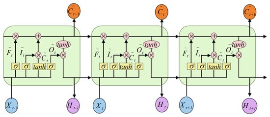
The LSTM is a representative gated recurrent architecture designed to address long-range dependencies. Standard recurrent networks may suffer from vanishing or exploding gradients during backpropagation through long sequences, which limits their ability to retain information over large time spans. By regulating information flow through gates and continuously updating the cell state, the LSTM alleviates these problems [17]. Its basic structure is shown in Figure 1.
Figure 1.
Schematic of the LSTM cell. Arrows indicate the direction of information flow; the blue, purple, and orange ellipses denote the input, hidden-state, and candidate cell-state vectors, respectively.
As shown in Figure 1, xt is the input at time t; Ct−1 and Ct are the previous and current cell states; ht−1 and ht are the previous and current hidden states; and ft, it, and ot denote the forget, input, and output gates, respectively. The state update equations are
ft = σ(Wf[ht−1,xt] + bf)
it = σ(Wi[ht−1,xt] + bi)
ot = σ(Wo[ht−1,xt] + bo)
ht = ot ⊙ tanh(Ct)
Through the coordinated action of the forget, input, and output gates, the LSTM selectively retains, writes, and exposes information. This mechanism enables the network to capture long-term temporal dependencies and makes it well suited to dynamic prediction problems with complex sequential characteristics.
2.2. Fundamentals of GA and DOA
The genetic algorithm is a population-based global optimizer inspired by biological evolution. Candidate solutions are encoded as chromosomes and evolved through selection, crossover, and mutation, with fitness values used to rank individuals and guide the population toward the global optimum [24]. The GA is gradient-free and broadly applicable, but it may converge prematurely in high-dimensional multimodal problems and can incur a high fitness evaluation cost. It is therefore often combined with an optimizer that has stronger local exploitation capability.
The dhole optimization algorithm was proposed by Mohammed et al. [20]. It maps the vocal communication, cooperative tracking, encirclement, and attack behavior of a dhole pack onto population position updates. Here, “attack” is the terminology inherited from the original DOA and denotes an exploitation-oriented position update stage in the optimization process, rather than a physical operation in the aero-engine model. The original method consists of initialization, exploration, and attack stages, in which prey position and prey intensity regulate the direction and step size of each individual. The original search and attack equations, together with the modifications proposed here, are presented in Section 2.3.
2.3. GA-DOA Hybrid Optimization Strategy
To preserve the behavioral structure of the original DOA while strengthening global exploration, a dual-population GA mechanism is embedded into the initialization–exploration–attack chain. In Stage I, GA and DOA populations evolve in parallel. DOA retains the original hunting member, hunting duration, exploration, and attack mechanisms, while a global optimum pool (GOP), a coevolution-scale decay factor, dual-mode position updates, greedy selection, and periodic elite exchange are introduced. The GA continuously injects diversity through crossover and mutation and transfers high-quality candidates to the DOA. In Stage II, the optimal output weights obtained in Stage I are fixed, and an independent DOA population locally refines the LSTM structural hyperparameters [20].
2.3.1. Initialization and Fitness Evaluation
Each GA-DOA individual Yi jointly encodes the loss weights for exhaust gas temperature T5 and thrust F, together with the sliding window length, the numbers of hidden units in the two LSTM layers, and the dropout rate. Let N be the population size, dim the problem dimension, and lbj and ubj the lower and upper bounds of the jth decision variable. Both populations are randomly initialized within the prescribed search space:
Y(i,j) = lbj + rand(ubj − lbj), j = 1,2,…,dim
Here, rand is uniformly distributed on [0,1]. After initialization and every position update, the output weights are normalized such that wT5 + wF = 1. The window length and hidden unit numbers are rounded and clipped to their admissible ranges. The validation set weighted mean square error is used as the fitness function:
where wT5 and wF are the loss weights for T5 and F, and MSET5 and MSEF are the corresponding validation set mean square errors. For either output variable, the validation error is
where Nval is the number of validation samples and yipred and yitrue denote the predicted and true values of sample i, respectively. GA-DOA minimizes fitness; a lower value indicates a better candidate.
Fitness = wT5MSET5 + wFMSEF, wT5 + wF = 1
2.3.2. Exploration Stage and GOP Guidance
During exploration, the search intensity is represented by the number of hunting members nhunt, which is randomly selected between 5 and 20. This range follows the original DOA formulation of Mohammed et al. [20] and is retained here without task-specific retuning so that the basic behavioral mechanism of DOA is preserved:
nhunt = round(5 + 15rand)
The hunting duration thunt is determined by nhunt and an environmental factor EF:
EF ∈ [0,1] characterizes the environmental favorability for hunting. In the original DOA, the target is the mean of the local best position plocal and global best position pglobal:
The vocalization variable is sampled randomly in [0,1]. Following the original DOA formulation [20], the fixed threshold of 0.5 is retained to switch between the exploration/encirclement branch and the attack branch; this threshold was not independently tuned for the present JT9D identification task. When the vocalization value is below 0.5, the algorithm enters exploration. If nhunt < 10, the individual approaches the target using the contraction factor C2:
If nhunt ≥ 10, encirclement is simulated by randomly selecting another individual z for the update:
The original DOA linearly decreases the search step according to
Although these rules reproduce search and encirclement behavior, the target is formed by a simple average, and the inner DOA schedule is not synchronized with the outer GA-DOA coevolution process. This may introduce guidance bias and population homogenization. A GOP is therefore constructed from high-quality candidates generated by both populations, and the best member in the pool replaces the averaged target:
P* denotes a candidate in the GOP and ptarget is the target position for the current coevolution generation. The decay schedule is further elevated to the outer coevolution scale:
The GOP stores at most five elite candidates. A new candidate is added when space is available; otherwise, it replaces the worst member only if its fitness is lower. For candidates with nearly identical output weight vectors, only the better one is retained. The best GOP member is used as the current DOA target.
where t and Tmax are the current and maximum coevolution generations. The modified DOA switches with equal probability between exploitation and exploration. In exploitation mode, an individual adaptively moves toward the GOP target:
In exploration mode, Gaussian perturbation enlarges the search coverage around the current solution:
A greedy rule accepts a candidate only when its fitness is lower than that of the current position. The GOP improves target quality, the outer-scale decay factor synchronizes exploration and exploitation, and the dual-mode updates and greedy selection improve escape from local optima and stabilize the iteration.
2.3.3. Attack Stage and Local Exploitation
After search and encirclement, a vocalization value greater than or equal to 0.5 activates the attack stage, consistent with the phase-switching rule of the original DOA [20]. In optimization terms, this stage performs exploitation around the identified prey/target rather than representing any physical engine process. The attack strategy is selected by the prey intensity factor η:
fitnessi and fitnessp are the fitness values of the current individual and the target, respectively. For η > 2, the prey is regarded as strong and a weakened prey vector wp is first constructed:
where plocal is the best position in the current population. A sine–cosine mixed perturbation then models repeated cooperative attacks:
For η ≤ 2, the prey is regarded as weak and a concentrated attack is applied:
The strong prey strategy maintains local search activity through periodic perturbation, whereas the weak prey strategy contracts the movement range and accelerates convergence. Both updates are retained, but their candidates are processed by common boundary handling, GOP updating, and greedy selection, preventing inferior solutions from propagating unconditionally and improving late-stage exploitation accuracy.
2.3.4. GA Crossover and Mutation
At each coevolution generation, the GA and DOA populations are updated in parallel. GA preserves the fittest elite, selects parents using tournaments of size two, and applies BLX-α crossover simultaneously in the weight and hyperparameter subspaces. The jth component of an offspring is generated as
where Yp1,j and Yp2,j are the jth components of the two parents and Δj = |Yp1,j − Yp2,j|. In this study, α = 0.5. Gaussian mutation is performed with probability Pm = 0.2:
where σ = 0.1 and UBj and LBj are the variable bounds. Continuous variables are clipped, the weights are renormalized, and discrete hyperparameters are rounded. The evaluated GA offspring are written to the GOP so that global discoveries immediately contribute to DOA target construction.
2.3.5. Dual-Population Coevolution and Elite Exchange
Stage I uses parallel GA and DOA populations. Each generation performs GA crossover and mutation and DOA exploration or attack, after which high-quality candidates from both populations are merged into the GOP. Every three generations, a bidirectional elite exchange with a ratio of 0.2 is performed. The best DOA individual replaces the worst GA individual only when it is fitter, and the reverse transfer follows the same conditional rule. This prevents detrimental exchanges while allowing for globally discovered regions and locally refined solutions to propagate between populations. Stage I terminates when the maximum number of generations is reached or the global best has not improved for five consecutive generations.
2.3.6. DOA Refinement and Fitness Caching
After Stage I, the optimal GOP weights wT5 and wF are fixed. An independent DOA population of 15 individuals locally refines the sliding window length, the two hidden-layer sizes, and the dropout rate for at most 20 iterations. These settings were selected from preliminary experiments: increasing the refinement population or iteration number beyond this level no longer produced a consistent reduction in validation error and occasionally caused slight performance deterioration, while the search burden continued to increase. Hence, 15 individuals and 20 iterations were retained as an empirical compromise between refinement capability and offline optimization cost. The complete exploration, encirclement, attack, boundary handling, and greedy selection mechanisms are retained. The refinement result is accepted only when it improves the Stage I optimum, thereby preventing performance degradation.
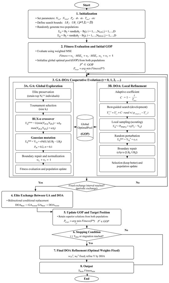
Because every fitness evaluation requires training an LSTM, a cache keyed by (sequence length, hidden1, hidden2, dropout rate, wT5, wF) is used. Revisited configurations return the cached result rather than retraining the network. The complete optimizer thus forms a progressive chain of original DOA exploration and attack, GOP-enhanced targeting, GA global exploration, greedy acceptance, bidirectional elite migration, and fixed-weight refinement, jointly improving search breadth, local accuracy, convergence stability, and computational efficiency. The overall procedure is shown in Figure 2.
Figure 2.
Flowchart of the GA-DOA algorithm.
2.3.7. Convergence Comparison of the Hybrid Algorithm
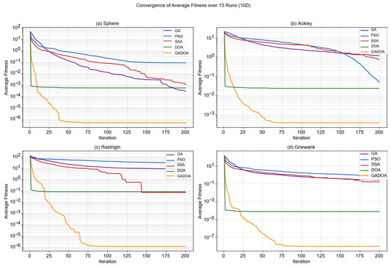
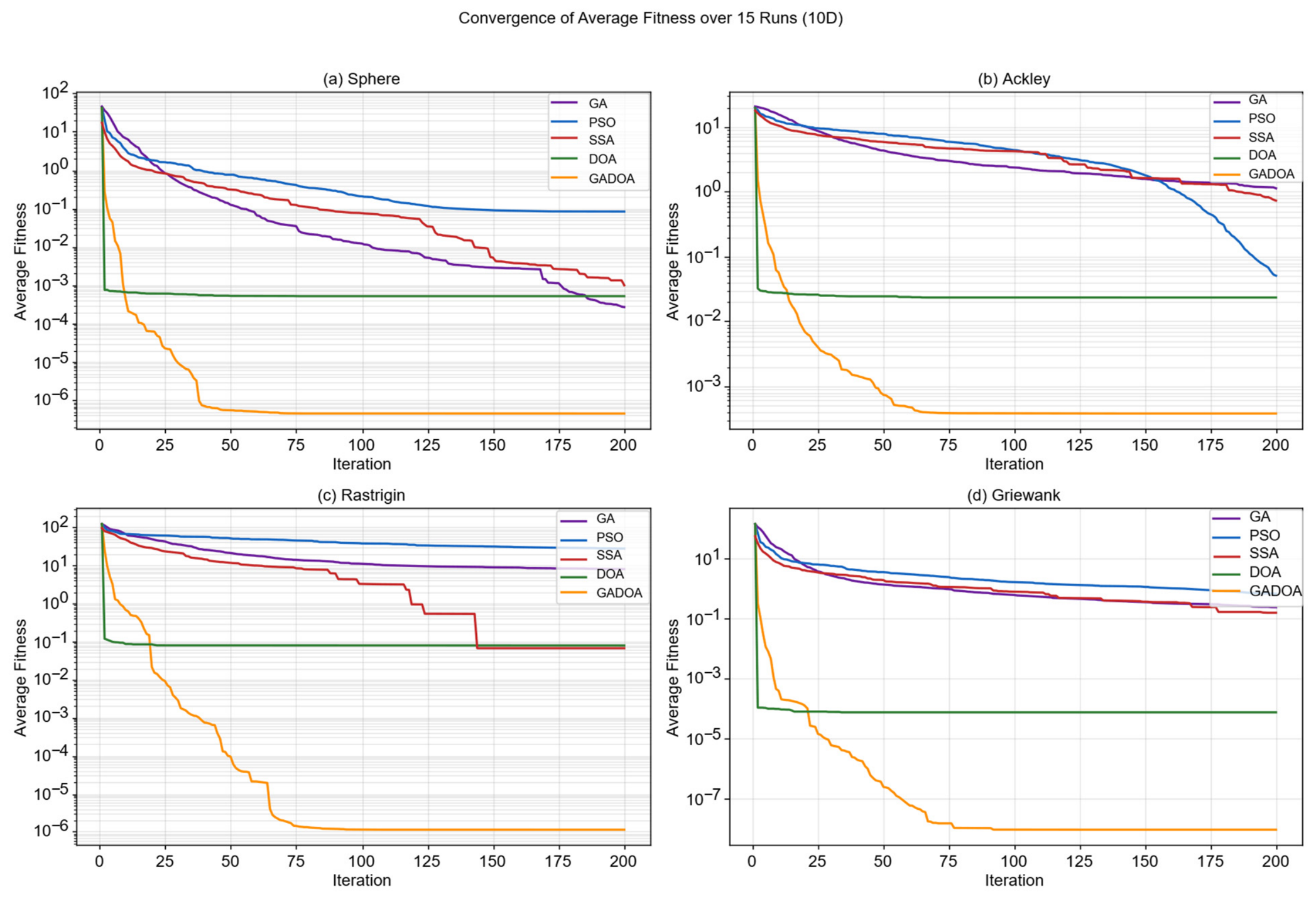
Sphere, Ackley, Rastrigin, and Griewank benchmark functions were used to assess the global and local search capability of GA-DOA. As shown in Figure 3, GA-DOA rapidly entered the low-fitness region during the early iterations and continued to improve smoothly. The 15-run statistics in Table 1 show that GA-DOA achieved the lowest mean final fitness on all four functions: 4.648 × 10⁻⁷ on Sphere, 3.853 × 10⁻⁴ on Ackley, 1.164 × 10⁻⁶ on Rastrigin, and 9.765 × 10⁻⁹ on Griewank. The corresponding mean rank is 1.00, followed by SSA (2.25), DOA (3.25), GA (3.75), and PSO (4.75). On Sphere, GA is the second-ranked method, whereas SSA is second on Ackley, Rastrigin, and Griewank. Thus, under the common 10-dimensional, population 20, 200-iteration setting, GA-DOA provides the best final solution accuracy among the five tested optimizers and shows a particularly large advantage on the multimodal functions. All five optimizers were executed 15 times with seeds 1–15, and Table 1 reports the mean and standard deviation of the final fitness. Because the available statistical summary provides mean and dispersion but not the run-level samples required to verify the previously stated Wilcoxon rank-sum p-values, the interpretation here is limited to the reported descriptive statistics and the cross-function mean rank comparison. These benchmark results support the search effectiveness of the cooperative design; the corresponding engineering benefit is evaluated separately in the engine identification experiments in the subsequent Results and Discussion section.
Figure 3.
Convergence curves on four benchmark functions.
Table 1.
Statistical results on four benchmark functions over 15 independent runs.
3. Data Processing and Modeling
3.1. Dataset and Preprocessing
3.1.1. Dataset Description
The data were generated using a dynamic JT9D aero-engine model implemented with the Toolbox for the Modeling and Analysis of Thermodynamic Systems (T-MATS) [25]. The self-generated dataset contains steady, transient, and representative flight conditions.
Fifty-four flight operating points were defined over altitudes of 0–8 km in 1 km increments and Mach numbers of 0.1–0.6 in increments of 0.1. Each 10 s simulation used three cumulative acceleration segments starting from idle. Accelerations began at 2.0, 4.5, and 7.0 s, each lasted 1.5 s, and were separated by 1 s steady intervals. With a time step of 0.04 s, each operating point/profile simulation contained 251 samples; across the three throttle profiles, each operating point therefore contributed 753 samples.
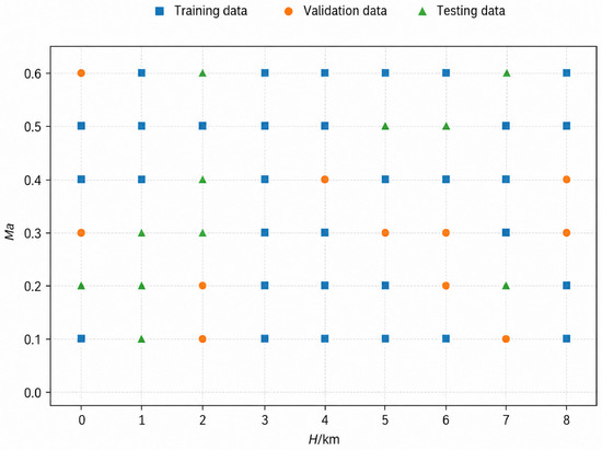
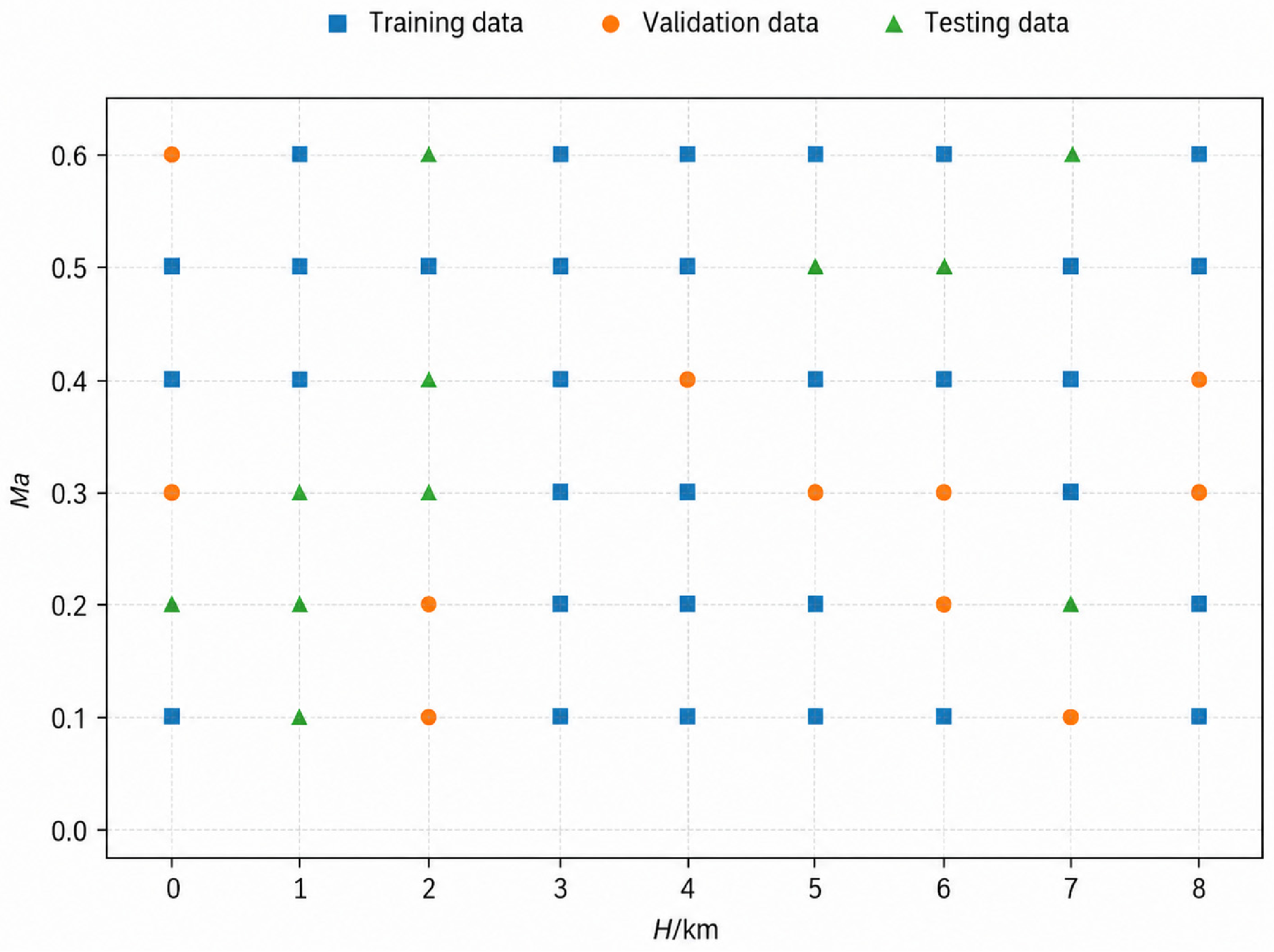
The dataset contains 11 SI unit variables: time (s), low-pressure spool speed N1 (rpm), high-pressure spool speed N2 (rpm), high-pressure compressor outlet total pressure Pt3 (Pa), combustor exit temperature T4 (K), fuel flow Wf (kg/s), low-pressure turbine exit temperature T5 (K), thrust F (N), altitude H (m), Mach number Ma, and signal type. N1, N2, Pt3, T4, and Wf were used as inputs, and T5 and F as outputs. With a fixed random seed (SEED = 42), the 54 operating points were randomly divided into training, validation, and test sets in a 6:2:2 ratio, corresponding to 32, 11, and 11 operating points. The distribution of operating points across the three sets is shown in Figure 4.
Figure 4.
Distribution of operating points in the training, validation, and test sets.
3.1.2. Data Preprocessing
Data preprocessing consisted of dataset splitting, sensor noise modeling, and normalization.
The 54 operating points were divided into training, validation, and test subsets using the fixed seed SEED = 42 and the 6:2:2 ratio described above, ensuring reproducibility.
To represent practical measurement uncertainty, output perturbations were introduced into the training and validation data before normalization, with σT5 = 3.0 K and σF = 0.75% × Fmean, where Fmean is the mean thrust in the training set. These values were selected as literature-informed, order-of-magnitude representations of thermocouple measurement and thrust determination uncertainty rather than as the specifications of particular sensors [26,27,28]. The test set remained noise free to provide an unbiased evaluation.
The input variables were standardized using the Z-score transformation
where μ and σ are the training set mean and standard deviation of each feature. The outputs were mapped linearly to [0,1] by min–max normalization:
where y is the original output and ymin and ymax are the minimum and maximum training values. All normalization parameters were computed from the training set and then applied unchanged to the validation and test sets to avoid data leakage. During training, multiplicative Gaussian noise with an amplitude of 0.001|x| was additionally applied to the inputs as implicit regularization.
3.2. Model Description
The physical JT9D system was represented by five input variables: low-pressure spool speed N1 (rpm), high-pressure spool speed N2 (rpm), high-pressure compressor outlet total pressure Pt3 (Pa), combustor exit temperature T4 (K), and fuel flow Wf (kg/s). The target outputs were low-pressure turbine exit temperature T5 (K) and thrust F (N).
N1 and N2 describe the spool speed state and are central to control law design; Pt3 reflects compressor pressure-raising capability and thermodynamic cycle efficiency; T4 characterizes the combustor thermal state; and Wf is the primary manipulated variable governing thrust. Together, these variables represent the thermodynamic state of the engine during acceleration. T5 and F are key indicators for performance assessment, control, fault diagnosis, and health management.
A two-layer LSTM was used as the base predictor [17]. This architecture was selected based on preliminary experiments conducted by our group before the present comparative study. In those experiments, increasing the network depth from one to two LSTM layers produced a clear improvement in dynamic prediction performance, whereas increasing the depth from two to three layers yielded only marginal additional gains and, for some evaluation metrics, even caused slight performance degradation. The two-layer architecture was therefore adopted as a practical balance between temporal feature representation and model complexity. Sliding window sequences were passed through two stacked LSTM layers and a fully connected output layer. Data from all 54 operating points were used to train one cross-condition model. Dropout regularization and early stopping were used to suppress overfitting and improve generalization [29,30].
3.3. Simulation Platform
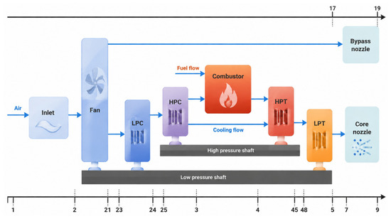
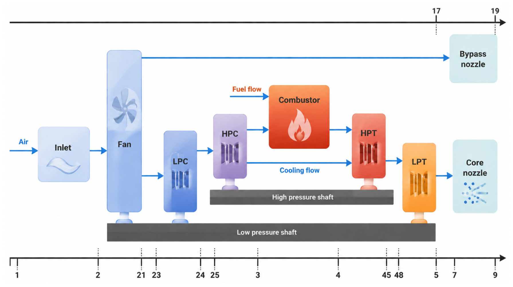
The component-level JT9D model was developed in MATLAB/Simulink using the open-source T-MATS v1.4.0 toolbox released by NASA [25], running in MATLAB/Simulink R2023a. It comprises an inlet, fan, low-pressure compressor, high-pressure compressor, combustor, high-pressure turbine, low-pressure turbine, core nozzle, and bypass nozzle. Standard station numbering is used, and common work equations are solved to obtain matched operating points. The station layout is shown in Figure 5.
Figure 5.
Station layout of the JT9D turbofan engine.
To generate multi-condition dynamic data over the flight envelope, the original model was extended only at the script level; the Simulink model, component maps, Newton–Raphson solver, and spool dynamics modules were not altered. Three extensions were introduced.
(1) Parameterized injection of flight environment conditions. In the original model, inlet total temperature Tt, total pressure Pt, and ambient static pressure Pamb were hard coded for a single design point. Before each run, the modified script computes the inlet conditions from altitude H and Mach number Ma using the ISA standard atmosphere:
Tt = Ta(1 + 0.2Ma2)
Ta and Pa are evaluated piecewise according to the ISA model. A lapse rate of L = 0.0065 K/m is used in the troposphere (H ≤ 11 km), and an isothermal value Ta = 216.65 K is used above this altitude [31]. The calculated quantities are written to Simulink constant blocks through set_param, extending the platform from one design point to batch simulations over H = 0–11 km and Ma = 0.1–0.8. Although the extended platform supports this broader envelope, the dataset used in this study was restricted to H = 0–8 km and Ma = 0.1–0.6.
(2) Programmatic generation of compound throttle commands. The original model used a single step command. The modified MATLAB script generates a 251-point speed command time series at 0.04 s intervals and supplies it to the Simulink input through a timeseries object. Each 10 s simulation starts from idle and applies three 1.5 s accelerations at 2.0, 4.5, and 7.0 s, successively reaching Nidle + Δ/3, Nidle + 2Δ/3, and Nmax = 3667.6 rpm, where Δ = Nmax − Nidle. One-second steady intervals are retained between acceleration segments. Step, linear ramp, and quadratic parabolic throttle profiles are included. To avoid divergence when the low-pressure spool leaves the component map boundary at high altitude and low speed, an adaptive idle speed schedule is used: Nidle = 3000 rpm for H ≤ 5 km, 3100 rpm for H = 6–8 km, 3200 rpm for H = 9–10 km, and 3300 rpm for H = 11 km.
(3) Standardized SI unit postprocessing. The original imperial unit outputs are retained in the model and converted by a separate Python script: F(lbf) × 4.44822→N, Wf(lbm/s) × 0.453592→kg/s, T(°R) × 5/9→K, and P(psia) × 6894.76→Pa. The resulting dataset is entirely expressed in SI units.
3.4. Modeling and Simulation
3.4.1. Model Hyperparameter Settings
Before training, the sliding window length, the numbers of hidden units in the first and second LSTM layers, and the dropout rate were jointly optimized by GA-DOA. The window length determines the accessible temporal context; too few hidden units may cause underfitting, whereas too many increase complexity and overfitting risk. Dropout suppresses feature co-adaptation by randomly deactivating neural connections during training [29].
The number of LSTM layers was not included as an additional GA-DOA decision variable in the present study. Although such an extension is theoretically feasible, it would introduce a discrete architecture dimension and substantially enlarge the hyperparameter search space. Because each fitness evaluation requires training an LSTM model, searching the network depth together with the window length, hidden unit numbers, dropout rate, and output loss weights would markedly increase the computational burden. Moreover, the main objective of this study is to evaluate the effectiveness of the proposed GA-DOA search mechanism under a controlled predictor architecture rather than to perform an exhaustive neural architecture search. Considering the preliminary depth comparison and the computational cost, the LSTM depth was therefore fixed at two layers, while the layer widths and other key hyperparameters were optimized. Incorporating network depth into the search space remains a feasible extension for future work.
The hidden layers used rectified linear units (ReLUs), whose nonsaturating positive region gradient helps alleviate gradient attenuation [32]. Training used the Adam optimizer, which adapts the update step from first- and second-moment estimates and is suitable for noisy nonstationary optimization [33]. Validation MSE was evaluated after each epoch. Training stopped when validation loss did not improve for 30 epochs, and the parameters from the best epoch were restored [30]. The optimized dropout layer and 0.1% multiplicative Gaussian input noise further improved robustness [29].
The hyperparameter search bounds were determined by combining guidance from previous LSTM hyperparameter tuning studies with the characteristics of the present dynamic identification task. Previous work has shown that LSTM performance is sensitive to architectural and temporal hyperparameters, including the number of hidden layers, the number of cell units, and the history time input, and has also emphasized the need to balance search effectiveness against computational resource constraints [34]. Accordingly, considering the relatively compact input–output dimension of the present problem, the temporal scale of the acceleration transients, the available data volume, and the repeated LSTM training cost incurred during metaheuristic optimization, the search ranges were restricted to physically and computationally reasonable intervals. The same bounds were used for all competing optimization algorithms to ensure a consistent search space.
3.4.2. Evaluation Metrics
Prediction accuracy was quantified by the root mean square error (RMSE), mean absolute error (MAE), and mean absolute percentage error (MAPE):
RMSE measures the overall magnitude of the prediction error.
MAE represents the average absolute deviation.
Here, N is the number of samples, and ŷi and yi are the predicted and true values. RMSE emphasizes the overall error scale, MAE describes the mean absolute bias, and MAPE quantifies relative error.
The comparison followed a controlled variable design: the LSTM backbone form, data split, training strategy, and hyperparameter search ranges were held constant, while the optimization method was varied among GA-DOA, GA, DOA, PSO, and SSA [20,21,22]. All optimized models used the same two-layer LSTM backbone and the same 54 operating points.
3.5. Results and Discussion
The models were implemented in Python 3.9.25. The original prediction curves and Table 2 and Table 3 retain the best validation run results for direct comparison with the initial experiments. To assess stochastic robustness and isolate mechanism contributions, an additional repeated-run study was conducted using a fixed data/noise split (split_seed = 42) and ten common run seeds for GA, DOA, the two ablated GA-DOA variants, and the complete GA-DOA. The repeated-run results are reported as mean ± sample standard deviation of RMSE and MAE.
Table 2.
Hyperparameter search space used for all optimization algorithms.
Table 3.
LSTM hyperparameter settings for the six models.
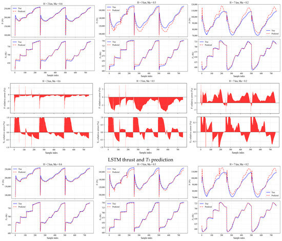
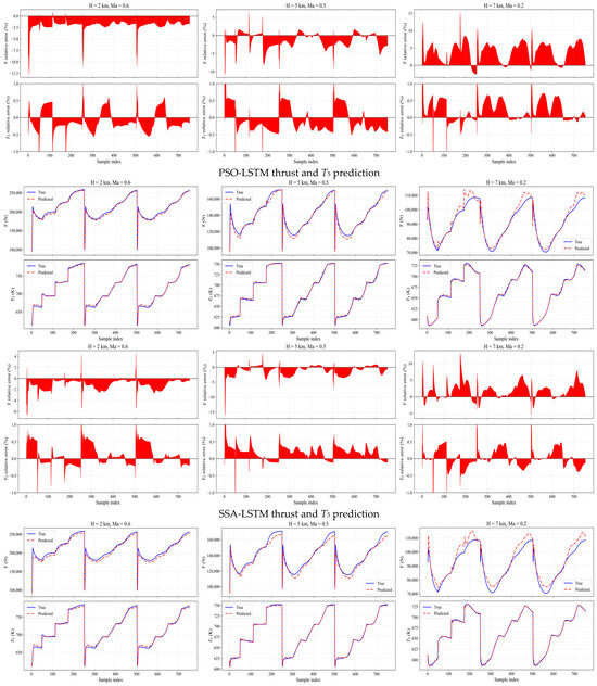
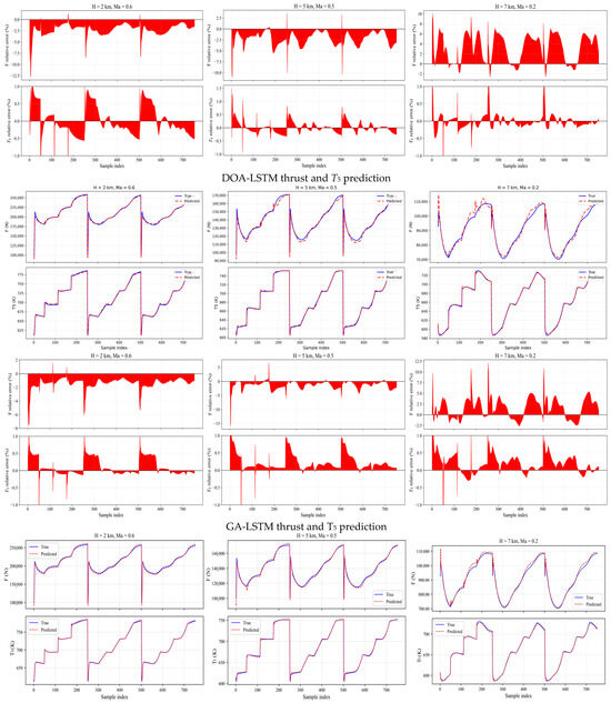
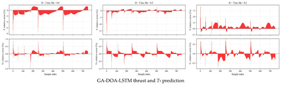
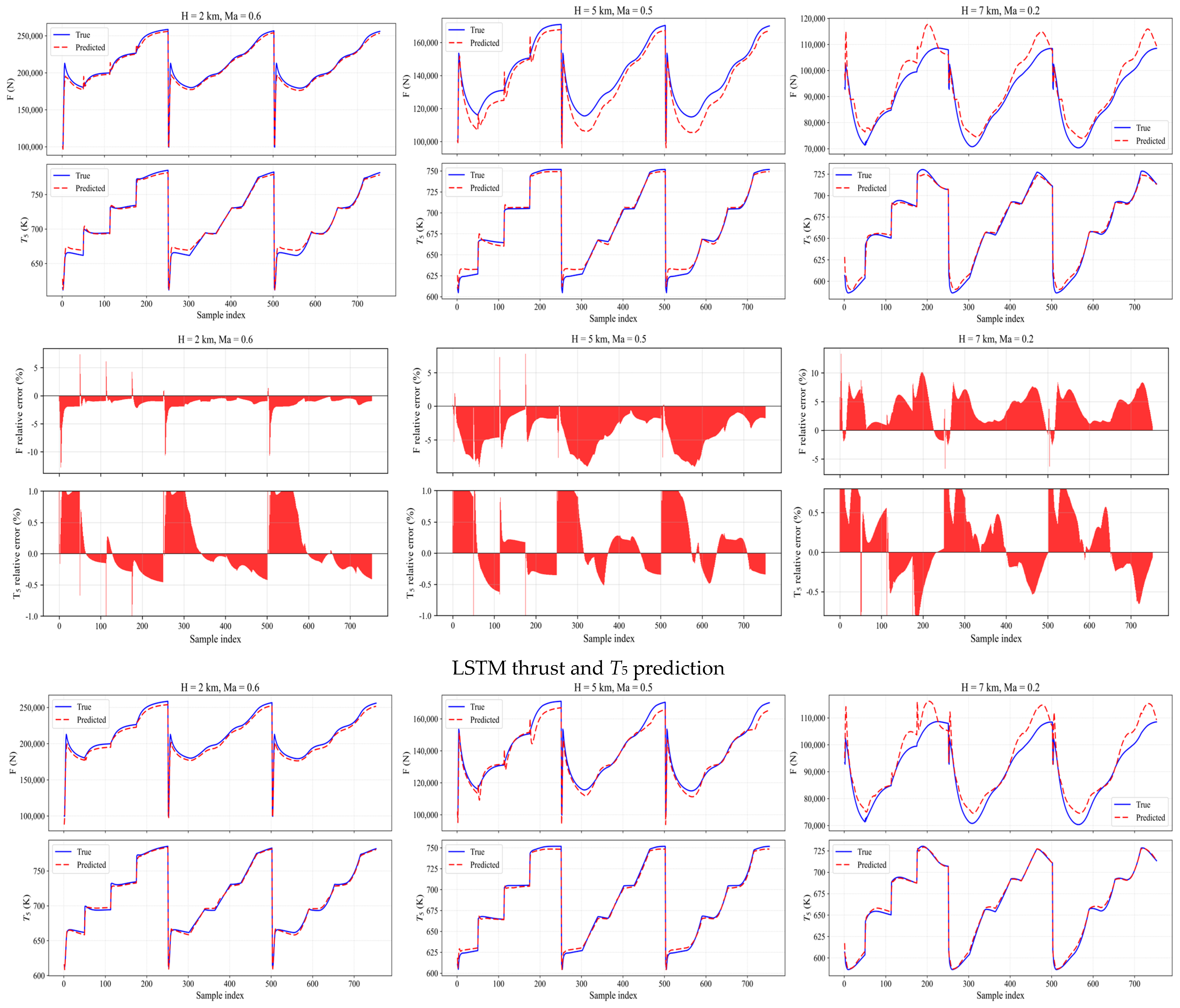
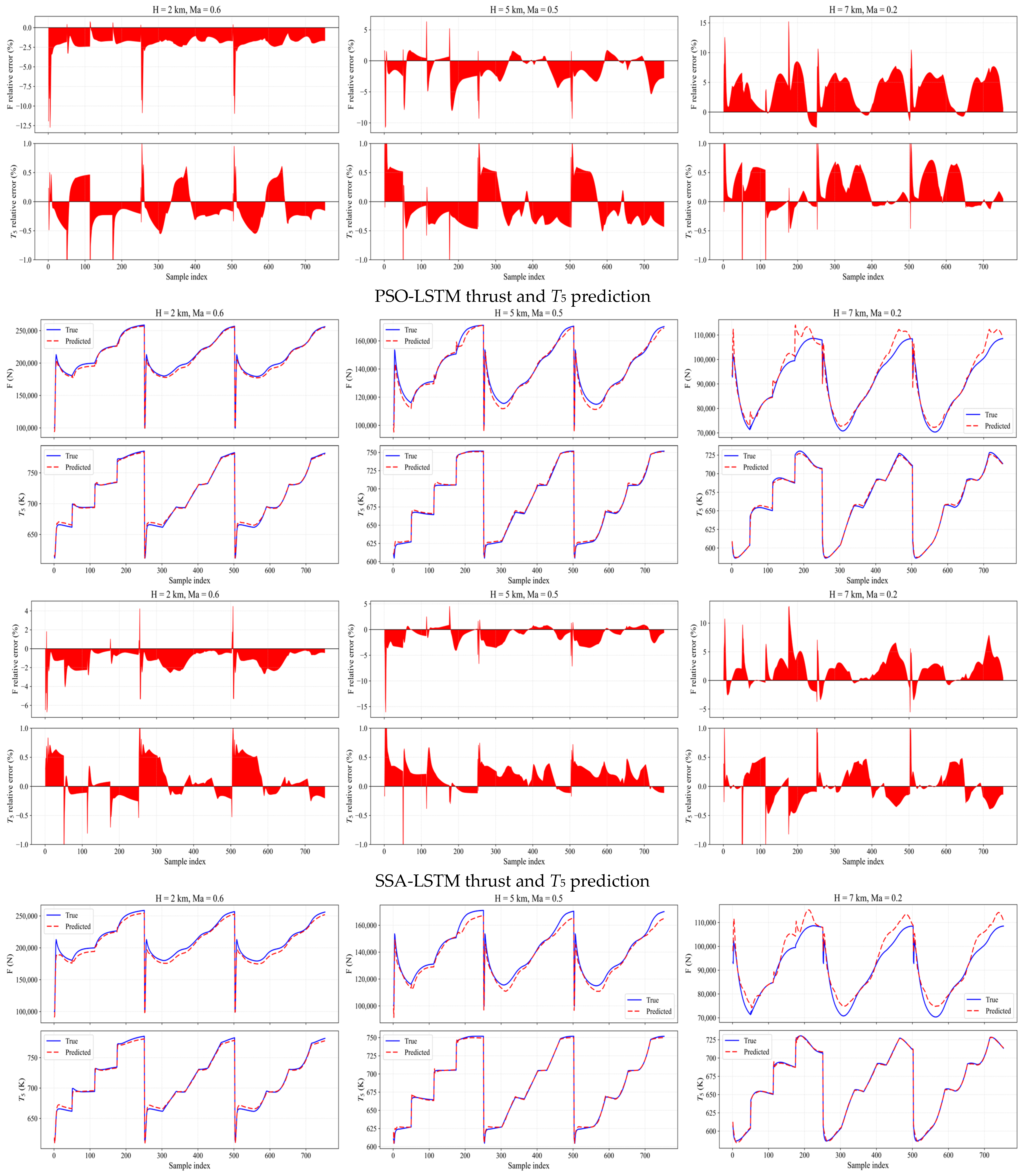
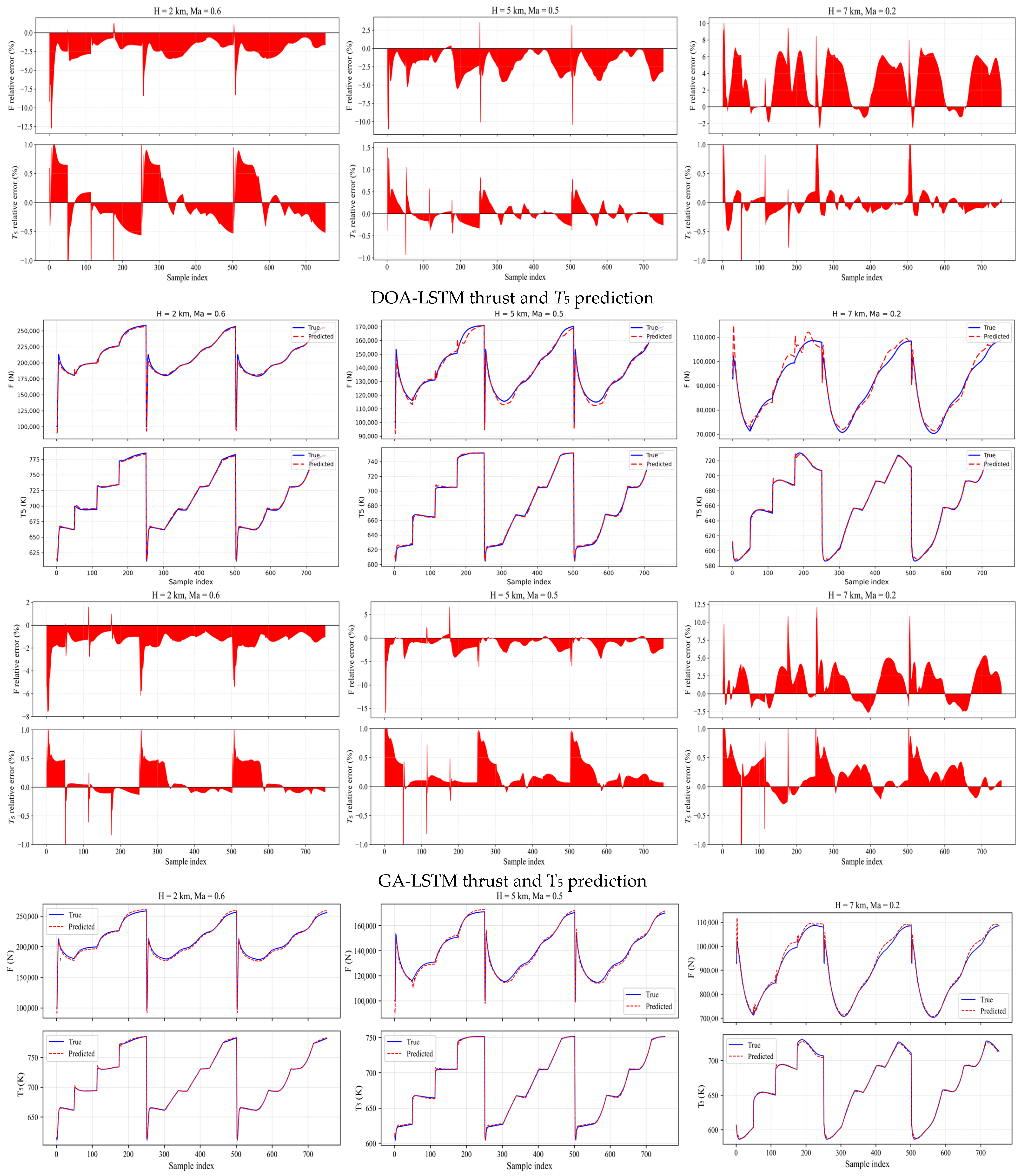
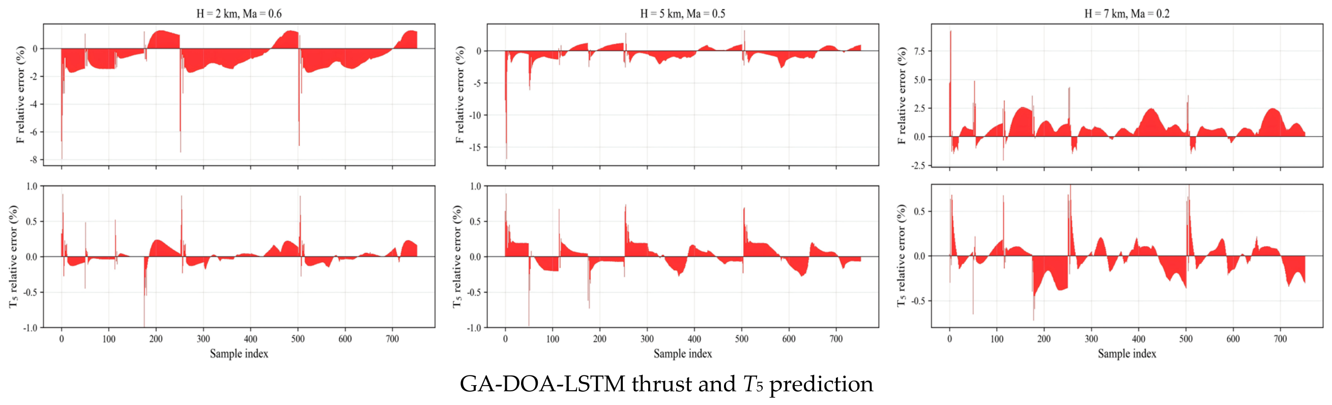
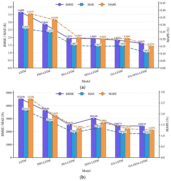
Three representative test conditions were selected from the 11 test operating points: a low-altitude/high-speed boundary condition (H = 2 km, Ma = 0.6), a high-altitude/low-speed boundary condition (H = 7 km, Ma = 0.2), and a moderate-altitude/moderate-speed condition (H = 5 km, Ma = 0.5). The first two represent distinct boundary regimes, while the moderate case is an interior condition; these curves are representative transient visualizations rather than an exhaustive survey of all altitude–Mach combinations. Figure 6 compares the thrust and T5 predictions of LSTM, PSO-LSTM, SSA-LSTM, DOA-LSTM, GA-LSTM, and GA-DOA-LSTM. GA-LSTM already tracks the reference thrust curves closely and removes much of the sustained deviation seen in the earlier baselines. GA-DOA-LSTM further lowers the full test set thrust RMSE from 2448.73 to 2430.10 N, MAE from 1864.57 to 1832.24 N, and MAPE from 1.3119% to 1.2576%, corresponding to reductions of 0.8%, 1.7%, and 4.1%, respectively. The pointwise advantage is not uniform at every instant: GA-LSTM remains locally competitive at H = 5 km and Ma = 0.5, but the aggregate metrics favor the cooperative optimizer. The comparison of error metrics for all six models is shown in Figure 7.
Figure 6.
Thrust and T5 predictions of the six models under representative operating conditions.
Figure 7.
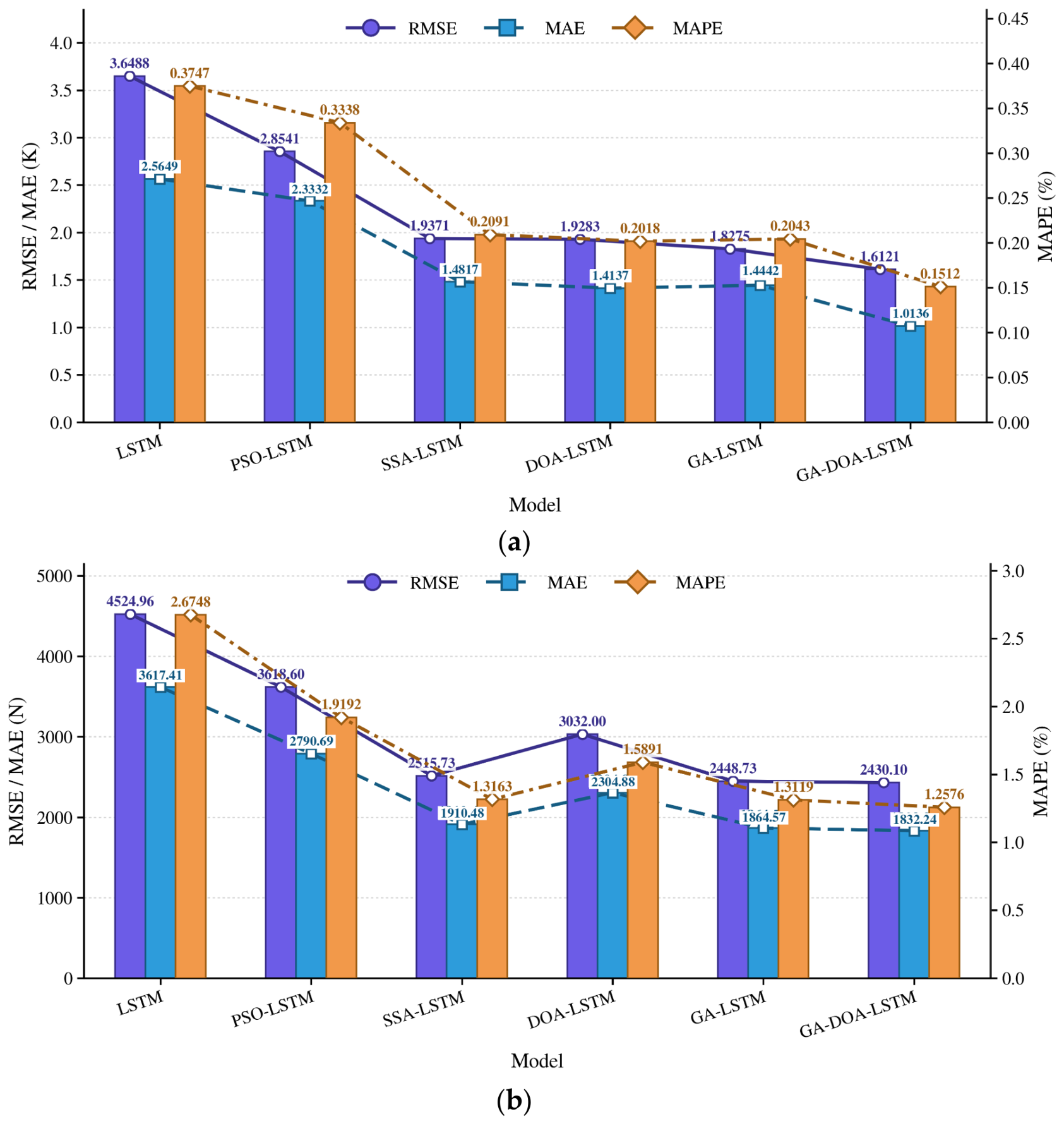
Comparison of error metrics for the six models: (a) T5 prediction performance; (b) thrust prediction performance.
The prediction of T5 was generally more accurate than that of thrust. GA-LSTM follows the T5 reference closely under all three conditions, with most deviations confined to short intervals around throttle transitions. GA-DOA-LSTM improves the full test set T5 RMSE from 1.8275 to 1.6121 K, MAE from 1.4442 to 1.0136 K, and MAPE from 0.2043% to 0.1512%, reductions of 11.8%, 29.8%, and 26.0%, respectively. The larger decrease in MAE than in RMSE indicates that the cooperative search mainly reduces persistent moderate errors, while a smaller number of transition-related peaks remain. The selected window and hidden layer configuration therefore improve temperature dynamic tracking without changing the overall response shape. At low altitude and high speed, larger fuel flow variation and thermal loading increase the difficulty of the problem; at high altitude and low speed, reduced air density and stronger thermal inertia slow the temperature response. The complete test-set prediction accuracy of the six models is summarized in Table 4.
Table 4.
Prediction accuracy of the six models on the test set.
Several error patterns were shared by all models. Thrust lag occurred during acceleration at H = 2 km, Ma = 0.6 and H = 5 km, Ma = 0.5, whereas overshoot was common at H = 7 km, Ma = 0.2. These similarities indicate that part of the prediction error originates from the inherent engine dynamics rather than from the learning algorithm alone.
At low and moderate altitudes, thrust lag is mainly associated with spool inertia and component rematching. After a throttle change, fuel flow and combustor heat release increase rapidly, but the high- and low-pressure spools require time to accumulate rotational energy. The compressor and turbine must also establish a new matched operating point, so thrust develops later than the control input.
A data-driven predictor must infer the future response from historical states. During a rapid transition from low to high power, the inputs may already have changed while thrust is still influenced by the preceding operating point. If this long-timescale dependence is not learned sufficiently, the model smooths the response and produces an apparent delay. This explains why different optimizers can show similar lag at the two lower-altitude conditions.
At H = 7 km and Ma = 0.2, the observed overshoot is related to the reduced ambient pressure and density, lower inlet mass flow, and delayed aerodynamic matching. Fuel addition initially increases heat release, while inlet and spool constraints postpone the establishment of the new steady state; consequently, turbine temperature and compressor outlet pressure may temporarily depart from their matched values and generate a thrust peak.
From the learning perspective, the high-altitude/low-speed response is highly nonstationary and underrepresented by boundary condition samples. Strong initial trends in fuel flow and spool acceleration may cause the model to anticipate the high-thrust state before aerodynamic matching and inertia have taken effect, resulting in a temporary overprediction.
3.5.1. Repeated-Run Robustness and Ablation Analysis
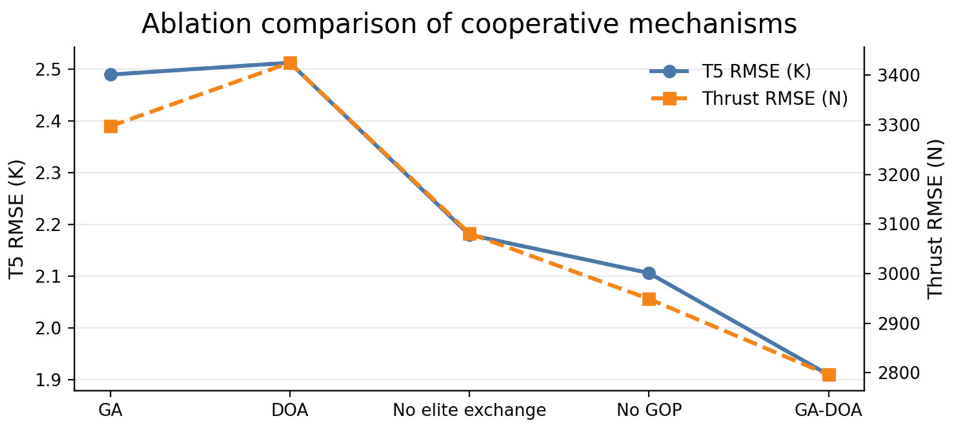
Because population-based optimizers are stochastic, single-run results may be sensitive to random initialization and search updates. Therefore, five variants—GA, DOA, GA-DOA without elite exchange (GADOA_no_elite), GA-DOA without GOP guidance (GADOA_no_GOP), and the complete GA-DOA—were independently repeated ten times. The data partition and sensor noise realization were fixed with split_seed = 42, while the same run seed sequence was used for all variants. This protocol isolates optimizer-induced variability and enables direct comparison of metric dispersion.
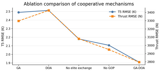
As summarized in Table 5 and Figure 8, the complete GA-DOA achieved the lowest mean error for all four repeated-run metrics, with T5 RMSE and MAE of 1.909 ± 0.618 K and 1.395 ± 0.531 K, respectively, and thrust RMSE and MAE of 2796 ± 479 N and 2077 ± 396 N, respectively. Compared with the pure GA baseline, the complete framework reduced the mean T5 and thrust RMSE by 23.3% and 15.2%, respectively. Compared with the pure DOA baseline, the corresponding reductions were 24.0% and 18.4%. These comparisons show that the observed improvement cannot be attributed to either GA or DOA operating independently but is associated with their integration and the accompanying cooperative mechanisms.
Table 5.
Ten-run robustness and ablation results (mean ± sample standard deviation).
Figure 8.
Comparison of mean T5 and thrust RMSE for the repeated-run robustness and ablation variants.
The ablation analysis focused on GOP guidance and bidirectional elite exchange because they represent two core cross-population cooperation mechanisms in the proposed framework. The GOP aggregates high-quality candidates generated by both populations and provides a shared search target, whereas bidirectional elite exchange directly transfers promising solutions between the GA and DOA populations. The component removal variants therefore evaluate two complementary forms of information sharing: shared target guidance and direct solution migration. Removing GOP guidance increased T5 RMSE and MAE by 10.3% and 16.6%, respectively, and increased thrust RMSE and MAE by 5.5% and 6.1%. These changes are consistent with the intended role of the GOP in improving the quality of the search target. Removing elite exchange increased T5 RMSE and MAE by 14.2% and 16.6%, respectively, and increased thrust RMSE and MAE by 10.2% and 10.3%. This result indicates that the conditional transfer of elite solutions facilitates the propagation of useful information between the two populations. Under the present experimental setting, elite exchange produced a somewhat larger reduction in mean error than GOP guidance, particularly for thrust prediction.
Overall, the results support three conclusions. First, GA alone does not account for the accuracy improvement of the complete method. Second, integrating GA and DOA provides better average prediction accuracy than using either optimizer independently. Third, removing either GOP guidance or bidirectional elite exchange increases the mean prediction errors, indicating that both shared target guidance and direct solution migration make positive marginal contributions when the remaining components of the framework are retained.
3.5.2. Fixed-Budget Fairness Analysis
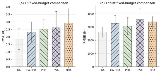
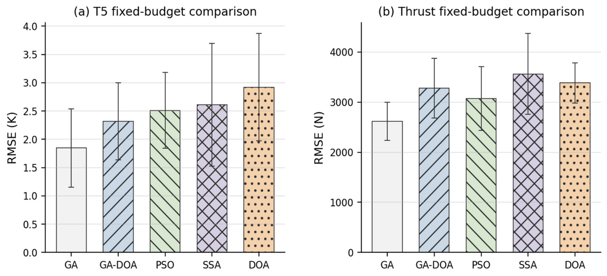
Table 6 and Figure 9 present a separate comparison. To further examine whether the observed gains were simply caused by a larger optimization budget, a separate fixed-budget comparison was performed in which GA, GA-DOA, PSO, SSA, and DOA were each limited to 120 fitness evaluations and repeated 10 times using the same data split and run seed sequence. Under this deliberately tight budget, GA obtained the lowest mean errors (T5 RMSE 1.847 ± 0.692 K; T5 MAE 1.397 ± 0.707 K; thrust RMSE 2917 ± 379 N; thrust MAE 2125 ± 308 N), while GA-DOA achieved 2.321 ± 0.681 K, 1.705 ± 0.585 K, 3274 ± 595 N, and 2469 ± 501 N, respectively. GA-DOA nevertheless remained more accurate than PSO, SSA, and DOA for T5 under the same evaluation budget, and outperformed SSA and DOA for thrust. These results show that the cooperative GA-DOA framework is not inherently advantaged by evaluation count and that its full accuracy benefit requires sufficient room for the coevolution, information exchange, and refinement stages to operate. In practical terms, the method trades a limited amount of additional offline optimization effort for higher final prediction accuracy in the full search configuration; this extra cost is confined to model development and does not increase online inference complexity.
Table 6.
Fixed-budget comparison with 120 fitness evaluations (ten runs; mean ± sample standard deviation).
Figure 9.
Fixed-budget comparison of T5 and thrust RMSE across ten independent runs. Error bars denote sample standard deviation.
3.5.3. Out-of-Envelope Extrapolation Analysis
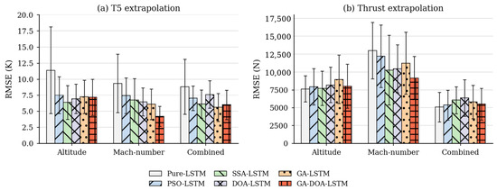
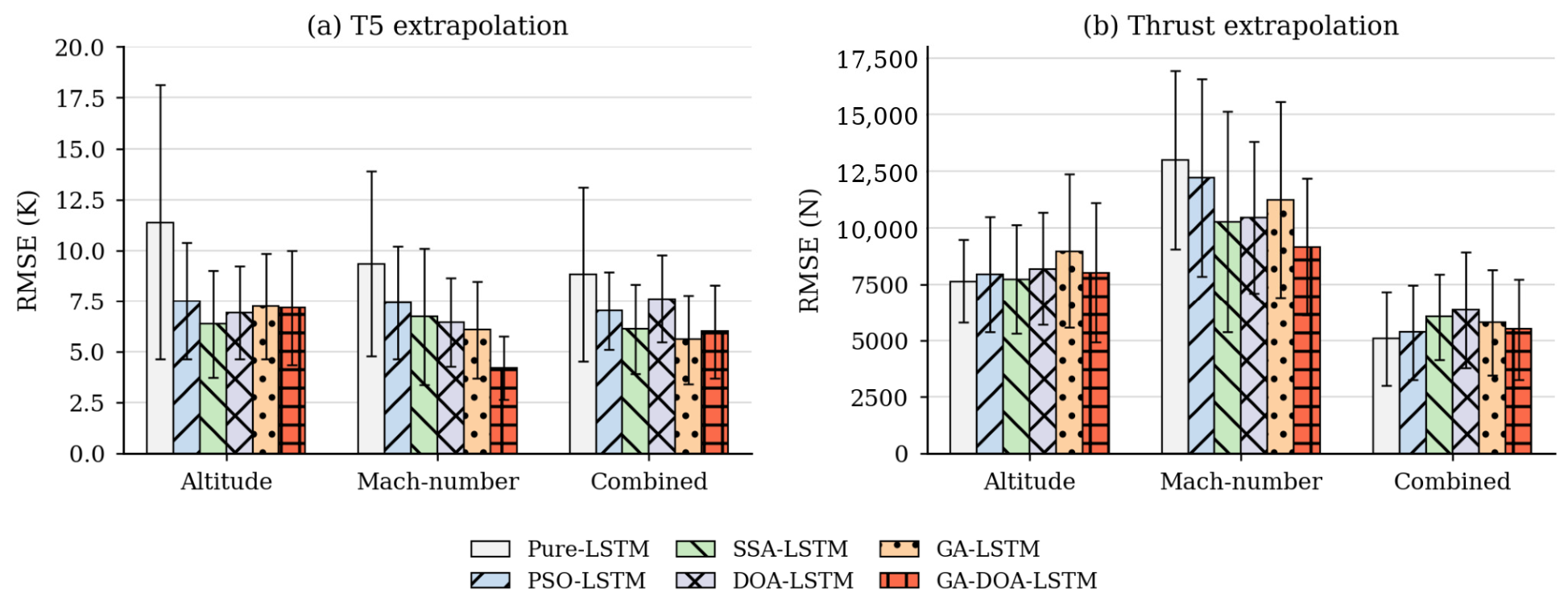
To assess extrapolation beyond the sampled operating envelope, additional tests were conducted outside the training domain of H = 0–8 km and Ma = 0.1–0.6. The extrapolation conditions were not selected arbitrarily. They were determined with reference to physically meaningful operating conditions of a transport turbofan engine and to the convergence boundary of the extended T-MATS/JT9D simulation model, so that the evaluation remained both operationally relevant and numerically feasible. Three categories were considered: altitude extrapolation, Mach number extrapolation, and combined altitude–Mach number extrapolation. The combined category explicitly includes high-altitude/high-speed conditions beyond both original boundaries, thereby testing the more demanding coupled distribution shift raised in the review. Low-altitude/low-speed cases are closer to the lower/interior portion of the sampled envelope and do not constitute the same simultaneous out-of-envelope shift. All extrapolation conditions were excluded from model training, validation, and hyperparameter optimization. The category-level RMSE statistics for six models over ten independent runs are summarized in Figure 10 and Table 7.
Figure 10.
Comparison of mean extrapolation RMSE for T5 and thrust under altitude, Mach number, and combined out-of-envelope conditions. Error bars denote the mean pointwise standard deviation across ten independent runs.
Table 7.
Extrapolation performance of different models beyond the training operating envelope.
For the two principal physical outputs, T5 and thrust, Table 7 also provides uncertainty intervals for the extrapolation results. Specifically, the bracketed values are averaged pointwise 95% confidence intervals derived from 10 independent runs. These intervals quantify the run-to-run uncertainty of the prediction errors for the main physical parameters and complement the mean ± standard deviation reporting. They should be interpreted as uncertainty intervals of the prediction error, rather than as measurement tolerances of the underlying T-MATS physical variables.
Across all 16 extrapolation operating points, GA-DOA-LSTM achieved an overall mean T5 RMSE of 5.767 K, which was 9.9% lower than the 6.399 K obtained by GA-LSTM. At the category level, GA-DOA-LSTM achieved the lowest T5 RMSE under Mach number extrapolation (4.21 K), a 30.7% reduction relative to GA-LSTM (6.08 K). The two methods were comparable under altitude extrapolation (7.17 K for GA-DOA-LSTM and 7.25 K for GA-LSTM), although SSA-LSTM produced the lowest altitude category value (6.36 K). Under combined extrapolation, GA-LSTM achieved the lowest T5 RMSE (5.60 K), compared with 6.00 K for GA-DOA-LSTM. These results show that the cooperative optimizer improves overall T5 extrapolation and provides a clear advantage for Mach number shifts but does not dominate every category.
Thrust extrapolation was more challenging and more condition dependent. GA-DOA-LSTM obtained the lowest category mean thrust RMSE under Mach number extrapolation (9145.5 N), compared with 12,984.1, 12,225.3, 10,256.6, 10,453.2, and 11,241.7 N for Pure LSTM, PSO-LSTM, SSA-LSTM, DOA-LSTM, and GA-LSTM, respectively. Relative to GA-LSTM, GA-DOA-LSTM reduced thrust RMSE by 10.5%, 18.6%, and 5.2% for altitude, Mach number, and combined extrapolation, respectively. It nevertheless did not attain the lowest thrust RMSE in the altitude or combined categories when all six models were compared. The larger errors at the most severe high-altitude conditions confirm that extrapolation remains limited by the absence of representative training information, particularly for thrust, which depends strongly on inlet conditions, airflow, component matching, and boundary region dynamics. Accordingly, the proposed method should be interpreted as improving resistance to specific operating envelope shifts rather than eliminating the general extrapolation limitation of data-driven identification. Future studies will expand physically representative training coverage near the engine operating and simulation convergence boundaries and investigate physics-informed and uncertainty-aware learning with higher-fidelity and experimental engine data.
The aggregate results in Table 2 and Table 3 support the visual comparison. For T5, GA-LSTM achieved an RMSE of 1.8275 K, an MAE of 1.4442 K, and a MAPE of 0.2043%; GA-DOA-LSTM reduced these values to 1.6121 K, 1.0136 K, and 0.1512%, respectively. Relative to GA-LSTM, the reductions were 11.8%, 29.8%, and 26.0%. For thrust, GA-LSTM obtained an RMSE of 2448.73 N, an MAE of 1864.57 N, and a MAPE of 1.3119%, whereas GA-DOA-LSTM achieved 2430.10 N, 1832.24 N, and 1.2576%. The corresponding gains over GA-LSTM were smaller but consistent at 0.8%, 1.7%, and 4.1%. This contrast indicates that adding DOA-based cooperative search to GA provides its clearest benefit for temperature prediction, while GA alone had already located a strong thrust model configuration. GA-DOA-LSTM nevertheless achieved the lowest RMSE, MAE, and MAPE for both outputs among all six models.
Overall, GA-DOA-LSTM achieved the best balance between accuracy and robustness for repeated aero-engine acceleration. Its performance remained stable across the evaluated test data, including the high-altitude boundary condition, supporting its use in engine state monitoring and health management applications.
4. Conclusions
A GA-DOA-LSTM framework was developed for dynamic identification of a high bypass ratio turbofan engine. The optimizer combines GA-based diversity preservation with the exploration and attack mechanisms of DOA, while the GOP, greedy acceptance, conditional elite exchange, and fixed-weight refinement improve target quality and late-stage convergence.
Using dynamic data from 54 T-MATS/JT9D operating points, the proposed model outperformed the baseline and four single-optimizer LSTM models on the in-envelope test set. It achieved T5 RMSE, MAE, and MAPE values of 1.6121 K, 1.0136 K, and 0.1512%, and thrust values of 2430.10 N, 1832.24 N, and 1.2576%, respectively. Additional out-of-envelope tests showed the accuracy degradation expected for data-driven models under distribution shift. In the expanded six-model comparison, GA-DOA-LSTM achieved the lowest category mean T5 and thrust RMSE under Mach number extrapolation. Averaged across all 16 extrapolation conditions, its T5 RMSE was 9.9% lower than that of GA-LSTM, and its thrust RMSE was lower than GA-LSTM in all three extrapolation categories. GA-LSTM nevertheless achieved the lowest T5 RMSE under combined extrapolation, and other baselines remained superior in some altitude and combined thrust cases. The proposed cooperative optimization therefore improves robustness to specific operating envelope shifts but does not remove the fundamental extrapolation limitations of data-driven modeling.
The present study has several limitations. First, the validation is based on the T-MATS/JT9D simulation environment, and a simulation-to-real discrepancy remains unavoidable. Real engine measurements may additionally be affected by component deterioration and variability, sensor and actuator uncertainty, environmental disturbances, and unmodeled thermal/mechanical dynamics; therefore, the present results should be interpreted as simulation-based validation rather than direct validation on a physical engine. Rig or flight test data will be used in future work to evaluate and, if necessary, reduce this simulation-to-real gap. Second, because the current model is developed for the JT9D configuration, its direct transferability to engines with different size, thrust class, bypass ratio, or architecture has not yet been established. Cross-engine validation and transfer learning strategies will therefore be investigated. Third, the cooperative GA-DOA procedure introduces additional offline optimization overhead because two search populations, information exchange, GOP maintenance, and final refinement are involved. This additional cost is paid during model development to obtain improved final predictive performance and does not increase the online inference complexity of the trained two-layer LSTM. Future work will investigate more computationally efficient search and surrogate-assisted optimization while preserving the accuracy benefit.
Author Contributions
Conceptualization, W.W. and Y.C.; methodology, Y.C. and W.W.; software, Y.C.; validation, Y.C., J.P., N.J. and Y.Z.; formal analysis, Y.C.; investigation, Y.C. and X.D.; resources, W.W.; data curation, Y.C. and X.D.; writing—original draft preparation, Y.C.; writing—review and editing, W.W. and J.P.; visualization, Y.C.; supervision, W.W.; project administration, W.W.; funding acquisition, W.W. All authors have read and agreed to the published version of the manuscript.
Funding
This research was funded by the Natural Science Basic Research Program of Shaanxi (Program No. 2026JC-YBMS-0529).
Data Availability Statement
The dataset was generated from the JT9D dynamic simulation implemented in T-MATS and contains 54 flight operating points. Each operating point/profile simulation contains 251 time steps, corresponding to 753 samples per operating point across the three throttle profiles. Because the data include internal simulation model configurations subject to confidentiality restrictions, the raw dataset is not publicly available. Experimental code and optimized model parameters may be obtained from the corresponding author upon reasonable request. All experiments used a fixed data split seed of 42. Within each comparative experiment, the evaluated methods used a common set of run seeds, while the run seed sets could differ across the main, ablation, fixed-budget, and extrapolation experiments.
Conflicts of Interest
The authors declare no conflicts of interest.
References
- Liu, D.X.; Jin, J. Development and challenges of aero-engine technology. Acta Aeronaut. Astronaut. Sin. 2022, 43, 025546. [Google Scholar]
- Xiao, D.; Song, S.; Xiao, H.; Wang, Z. Predicting the performance status of aero-engines using a spatio-temporal decoupled digital twin modeling method. Adv. Eng. Inform. 2025, 65, 103218. [Google Scholar] [CrossRef] [Scilit]
- Zheng, Q.G. Aero-Engine Performance Optimization Control Based on Nonlinear Model Predictive Control. Ph.D. Dissertation, Nanjing University of Aeronautics and Astronautics, Nanjing, China, 2023. [Google Scholar]
- Fan, Z.Y.; Wang, Z.L.; Liu, Z.X. Prediction model on aircraft engine performance parameters based on XGBoost. Comput. Meas. Control 2023, 31, 46–52. [Google Scholar]
- Liao, Z.; Zhang, R.; Zhao, H.; Gao, F.; Geng, J.; Chen, X.; Song, Z. Towards domain shifts: Stream fine-tuning via feed-forward fault data generation for on-board aero-engine gas-path diagnosis. Measurement 2024, 237, 115207. [Google Scholar] [CrossRef] [Scilit]
- Wang, W.; Li, J.F.; Liu, S. Nonlinear identification of aero-engine transient states based on an improved local linear model tree. Inf. Control 2020, 49, 560–569, 577. [Google Scholar]
- Asgari, H.; Ory, E. Machine learning approaches for modelling a single shaft gas turbine. Int. J. Model. Identif. Control 2021, 37, 275–284. [Google Scholar] [CrossRef] [Scilit]
- Vu, D.Q.; Razakarivony, S.; Thepaut, S.; Doquet, G.; Marnissi, Y.; Nocture, M. Aircraft engine performance estimation from multi-point and multi-time operational data via neural networks. In Proceedings of the 2024 IEEE Conference on Artificial Intelligence (CAI), Singapore, 25–27 June 2024. [Google Scholar]
- Chen, Z.Q.; Hong, J.; Xiao, G.; Wen, X. Dynamic parameter identification of an aero-engine based on SSA-NARX. J. Eng. Therm. Energy Power 2024, 39, 205–215. [Google Scholar]
- Cui, Z.; Yan, Z.; Zhao, M.; Zhong, S. Gas path parameter prediction of aero-engine based on an autoregressive discrete convolution sum process neural network. Chaos Solitons Fractals 2022, 154, 111627. [Google Scholar] [CrossRef] [Scilit]
- Wang, K.; Guo, Y.; Zhao, W.; Zhou, Q.; Guo, P. Gas path fault detection and isolation for aero-engine based on LSTM-DAE approach under multiple-model architecture. Measurement 2022, 202, 111875. [Google Scholar] [CrossRef] [Scilit]
- Liu, Y.; Chen, X.; Lin, Z.; Wang, Y.; Zhou, Q.; Qing, X. Aeroengine gas path parameter trend prediction based on LSTM. In Proceedings of the SAE 2023 Intelligent Urban Air Mobility Symposium, Hangzhou, China, 20 October 2023. [Google Scholar]
- Meng, W.; Pan, Z.; Wen, S.; Qin, P.; Sun, X. Aeroengine thrust estimation and embedded verification based on improved temporal convolutional network. Chin. J. Aeronaut. 2024, 37, 106–117. [Google Scholar] [CrossRef] [Scilit]
- Xiao, D.; Xiao, H.; Li, R.; Wang, Z. Application of physical-structure-driven deep learning and compensation methods in aircraft engine health management. Eng. Appl. Artif. Intell. 2024, 136, 109024. [Google Scholar] [CrossRef] [Scilit]
- Kim, S. Application of machine learning and its effectiveness in performance model adaptation for a turbofan engine. Aerosp. Sci. Technol. 2024, 147, 108976. [Google Scholar] [CrossRef] [Scilit]
- Hu, C.; Miao, K.; Zhou, M.; Shen, Y.; Sun, J. Intelligent performance degradation prediction of light-duty gas turbine engine based on limited data. Symmetry 2025, 17, 277. [Google Scholar] [CrossRef] [Scilit]
- Hochreiter, S.; Schmidhuber, J. Long short-term memory. Neural Comput. 1997, 9, 1735–1780. [Google Scholar] [CrossRef] [Scilit]
- Lin, L.; Liu, J.; Guo, H.; Lv, Y.; Tong, C. Sample adaptive aero-engine gas-path performance prognostic model modeling method. Knowl.-Based Syst. 2021, 224, 107072. [Google Scholar] [CrossRef] [Scilit]
- Ma, S.; Wu, Y.F.; Zheng, H.; Guo, L.F. Aero-engine gas-path parameter prediction based on an improved LSTM. Meas. Control Technol. 2024, 43, 1–10. [Google Scholar]
- Mohammed, B.O.; Aghdasi, H.S.; Salehpour, P. Dhole optimization algorithm: A new metaheuristic algorithm for solving optimization problems. Clust. Comput. 2025, 28, 430. [Google Scholar] [CrossRef] [Scilit]
- Eberhart, R.C.; Kennedy, J. A new optimizer using particle swarm theory. In Proceedings of the Sixth International Symposium on Micro Machine and Human Science; IEEE: Nagoya, Japan, 1995; pp. 39–43. [Google Scholar]
- Xue, J.; Shen, B. A novel swarm intelligence optimization approach: Sparrow search algorithm. Syst. Sci. Control Eng. 2020, 8, 22–34. [Google Scholar] [CrossRef] [Scilit]
- Shang, M.; Tian, M.; Wang, X. GA-DE: An integrated meta-heuristic approach for optimizing feedforward neural networks. J. Supercomput. 2025, 81, 339. [Google Scholar] [CrossRef] [Scilit]
- Holland, J.H. Adaptation in Natural and Artificial Systems; University of Michigan Press: Ann Arbor, MI, USA, 1975. [Google Scholar]
- Chapman, J.W.; Lavelle, T.M.; May, R.D.; Litt, J.; Guo, T.-H. Toolbox for the Modeling and Analysis of Thermodynamic Systems (T-MATS) User’s Guide; NASA/TM-2014-216638; NASA Glenn Research Center: Cleveland, OH, USA, 2014.
- George, B.; Muthuveerappan, N. Error estimation of measured exhaust gas temperature in afterburner mode in an aero gas turbine engine. Def. Sci. J. 2022, 72, 10–17. [Google Scholar] [CrossRef] [Scilit]
- SAE International. The Preparation and Use of Thermocouples for Aircraft Gas Turbine Engines; SAE Aerospace Information Report AIR46C; SAE International: Warrendale, PA, USA, 2022. [Google Scholar] [CrossRef] [Scilit]
- Gillespie, J.; Ng, W.; Lowe, K.T.; Crook, L.; Oechsle, V.L. Acoustic thrust estimation on turbofan engines. J. Propuls. Power 2023, 39, 130–140. [Google Scholar] [CrossRef] [Scilit]
- Srivastava, N.; Hinton, G.; Krizhevsky, A.; Sutskever, I.; Salakhutdinov, R. Dropout: A simple way to prevent neural networks from overfitting. J. Mach. Learn. Res. 2014, 15, 1929–1958. [Google Scholar]
- Prechelt, L. Automatic early stopping using cross validation: Quantifying the criteria. Neural Netw. 1998, 11, 761–767. [Google Scholar] [CrossRef] [Scilit]
- ISO 2533:1975; Standard Atmosphere. ISO: Geneva, Switzerland, 1975.
- Nair, V.; Hinton, G.E. Rectified linear units improve restricted Boltzmann machines. In Proceedings of the 27th International Conference on Machine Learning, Haifa, Israel, 21–24 June 2010; pp. 807–814. [Google Scholar]
- Kingma, D.P.; Ba, J. Adam: A method for stochastic optimization. In Proceedings of the International Conference on Learning Representations, San Diego, CA, USA, 7–9 May 2015. [Google Scholar]
- Dhake, H.; Kashyap, Y.; Kosmopoulos, P. Algorithms for hyperparameter tuning of LSTMs for time series forecasting. Remote Sens. 2023, 15, 2076. [Google Scholar] [CrossRef] [Scilit]

Disclaimer/Publisher’s Note: The statements, opinions and data contained in all publications are solely those of the individual author(s) and contributor(s) and not of MDPI and/or the editor(s). MDPI and/or the editor(s) disclaim responsibility for any injury to people or property resulting from any ideas, methods, instructions or products referred to in the content. |
© 2026 by the authors. Licensee MDPI, Basel, Switzerland. This article is an open access article distributed under the terms and conditions of the Creative Commons Attribution (CC BY) license.