Comparative Assessment of Random Forest and Linear Regression for Predicting South Asian Aridity Driven by Tropical Ocean Signals

Highlights

What are the main findings?

• ENSO strongly influences South Asian aridity, with asymmetric, threshold-dependent responses: extreme El Niño events disproportionately intensify aridity.
• Random Forest outperforms linear regression, with SHAP analysis identifying Niño3.4 as the dominant oceanic predictor of aridity.

What are the implications of the main findings?

• After removing long-term trends, interannual aridity predictability persists most strongly in hyper-arid and semi-arid dryland zones.
• Tropical ocean signals explain only modest year-to-year variability regionally, highlighting the need to incorporate local terrestrial processes for operational drought forecasting in South Asia.

Abstract

The South Asian monsoon sustains nearly one-quarter of the global population, yet the combined effects of water supply and atmospheric evaporative demand on regional aridity remain poorly integrated in long-term assessments. This study characterizes spatial and temporal aridity dynamics across the South Asian Monsoon region from 1901 to 2024 using the UNEP Aridity Index, offering a comprehensive view of hydroclimatic stress beyond precipitation alone. We integrate gridded climate observations with sea surface temperature records through Empirical Orthogonal Function decomposition and an interpretable machine learning framework, comparing linear regression against Random Forest and Hybrid models trained on historical data and validated independently. Our analysis reveals pronounced warming, spatially heterogeneous drying concentrated in northwestern regions, and a robust ENSO-aridity teleconnection modulated by the Indian Ocean Dipole. Machine learning models demonstrate superior skill in capturing nonlinear, threshold-dependent responses, yet their performance varies substantially across aridity zones, with linear approaches failing entirely in humid regions while hybrid frameworks excel in drylands. Critically, after removing long-term trends, interannual predictability persists most strongly in hyper-arid and semi-arid zones, where ENSO and IOD signals remain detectable, but declines elsewhere. SHapley Additive exPlanations identify Niño3.4 as the dominant oceanic predictor, with extreme El Niño events disproportionately intensifying aridity. These findings demonstrate that tropical ocean signals alone explain only modest year-to-year variability in the regional mean, with predictability concentrated in specific dryland zones. This work provides a diagnostic foundation for drought early-warning systems while emphasizing the need to incorporate local terrestrial processes and long-term trends for operational forecasting in one of the world’s most climate-vulnerable regions.

1. Introduction

South Asia’s water resources face increasing stress from changing precipitation and rising temperatures, with their combined effects on water availability and atmospheric evaporative demand contributing to increasing aridity across parts of the subcontinent [1]. The South Asian monsoon is the dominant climatic feature controlling the hydrological and agricultural cycles of this region. Its annual onset and variability influence the livelihoods of nearly one-quarter of the global population by replenishing rivers, aquifers, and croplands [2,3]. This variability is notoriously complex, manifesting not only from year to year but also at decadal scales, with profound consequences for the region’s densely populated and predominantly agrarian societies [4,5]). The monsoon’s spatial and temporal behavior defines sharp environmental contrasts from the humid forests of the northeast to the semi-arid and arid regions of northwestern India and Pakistan [6]. In these transitional and dryland zones, which include the Thar Desert and the rain-shadow regions of the Western Ghats, even slight deviations from normal rainfall can trigger widespread drought, threatening food security and rural livelihoods; [7]. In these drylands, small changes in water availability can have severe implications, making the understanding of regional aridity crucial.

Aridity arises from a persistent imbalance between water supply and atmospheric evaporative demand. It reflects the interaction among precipitation (P), potential evapotranspiration (PET), vegetation, and human activity [8,9]. Unlike drought, which is typically a temporary anomaly relative to climatic conditions, aridity represents a longer-term characteristic of climate and provides an important measure of regional water stress. This imbalance currently affects over one-third of the world’s population, contributing to crop failure, water scarcity, and land degradation [10,11]. Prolonged aridity may ultimately drive desertification, undermining agricultural productivity and ecosystem stability [12]. For South Asia, where a significant portion of the population depends on rain-fed agriculture for staples like wheat and rice, the implications of increasing aridity are particularly acute [13]. Quantifying and tracking aridity are therefore essential for climate adaptation and water-resource management, particularly in South Asia, where livelihoods are tightly linked to the land’s moisture balance.

The United Nations Environment Programme (UNEP) Aridity Index, defined as the ratio of P to PET, provides an integrated measure of this moisture balance and serves as the basis for defining global dryland classifications [14]. Because it accounts for both water input and evaporative demand, the UNEP Aridity Index can reveal ‘warming-induced drying,’ where increased temperatures intensify PET even without declines in rainfall [15,16]. Hence, aridity trends offer a more complete picture of hydroclimatic stress than precipitation changes alone, making the UNEP Aridity Index particularly useful for assessing hydroclimatic changes across regions with contrasting climatic regimes.

Among the large-scale climate drivers influencing South Asia’s hydroclimate, the El Niño–Southern Oscillation (ENSO) exerts the most prominent control [17,18]. El Niño events typically weaken monsoon circulation, causing reduced rainfall and widespread drought, while La Niña events tend to enhance rainfall [19,20]. However, this ENSO–monsoon relationship is known to be non-stationary and has weakened in recent decades, modulated by other modes of sea surface temperature variability. Notably, the Indian Ocean Dipole (IOD) plays a critical role, with a positive IOD often able to counter the drying effect of an El Niño, thereby restoring monsoon rains over the subcontinent [21].

Despite decades of research into these teleconnections, most existing predictability studies for South Asia have focused on forecasting seasonal monsoon rainfall totals using statistical models based on ENSO and IOD precursors [22,23]. Consequently, their integrated influence on aridity remains critically understudied. Focusing on aridity rather than rainfall alone is important because changes in atmospheric evaporative demand can intensify water stress even when precipitation changes are relatively modest. A more integrated assessment is therefore needed to determine how large-scale ocean variability is associated with spatial and temporal changes in South Asian aridity.

Advances in data-driven methods now enable more nuanced analyses of such complex, nonlinear relationships. Conventional linear approaches are useful for identifying broad statistical relationships but may not adequately represent nonlinear responses and interactions among multiple climate predictors. Machine learning (ML) approaches, especially ensemble algorithms such as Random Forests (RF), can capture intricate dependencies among multiple predictors without restrictive statistical assumptions [24]. Furthermore, explainable Artificial Intelligence tools such as SHapley Additive exPlanations (SHAP) provide transparent insights into the relative importance of individual drivers, allowing ML to function as both a predictive and diagnostic framework [25]. Because apparent predictive skill may partly reflect shared long-term trends rather than true interannual teleconnections, we additionally assess model performance after linear detrending to isolate the robustness of year-to-year ocean-driven signals.

To address these gaps, we integrate conventional hydroclimatic diagnostics with comparative machine learning and explainable artificial intelligence within a century-long framework (1901–2020). Specifically, we aim to (1) characterize long-term trends and spatial patterns of precipitation, temperature, PET, and the Aridity Index; (2) identify spatiotemporal modes linking tropical ocean variability to aridity; (3) compare Random Forest, Linear Regression, and Hybrid models for predictive skill; and (4) diagnose dominant predictors and distinguish trend-driven from interannual predictability. By shifting the focus from monsoon rainfall alone to the integrated metric of aridity, and by leveraging a century of hydroclimatic data with advanced machine learning approaches, this work offers new insights into the processes linking large-scale ocean variability and terrestrial water stress in South Asia. The results provide a basis for understanding the predictive potential of tropical ocean signals and for improving drought prediction and regional water and agricultural management strategies in a warming South Asia.

2. Data and Method

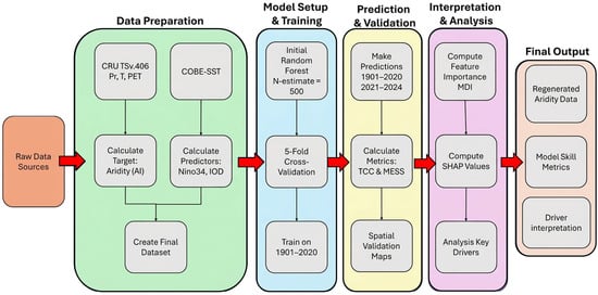
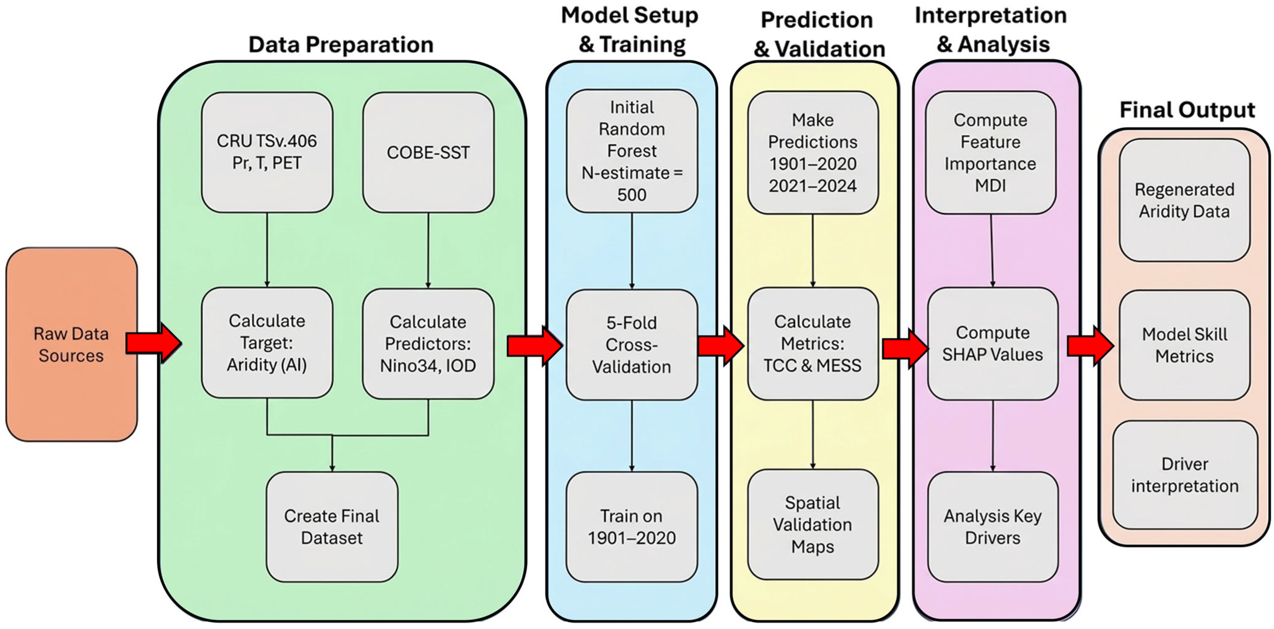
The overall analytical workflow for this study, integrating data processing, statistical analysis, and an explainable machine learning framework, is summarized in Figure 1.

Figure 1. Workflow diagram showing data sources, preprocessing steps, Random Forest model architecture, and explainable artificial intelligence framework for quantifying ENSO’s influence on South Asian aridity.

2.1. Study Region and Data Sources

For the purposes of this study, the South Asian (SAM) region was operationally defined as the geographical domain 60–103° E and 0–40° N, covering nine countries, i.e., Afghanistan, Bangladesh, Bhutan, India, Maldives, Myanmar, Nepal, Pakistan, and Sri Lanka. Climate variables including precipitation, daily mean temperature and potential evapotranspiration from 1901 to 2024 were obtained from the Climatic Research Unit (CRU TS v4.08) gridded dataset at 0.5° × 0.5° resolution (https://crudata.uea.ac.uk/cru/data/hrg/; accessed on 20 October 2025). These products have been well validated and frequently used in previous studies [26]. Widely recognized for its long-term consistency and reliability, CRU data have been extensively used in climate studies, including IPCC assessments [27]. Topographic data were obtained from the ETOPO1 Global Relief Model, a 1-arc-minute (~1.85 km) resolution global dataset that integrates land surface topography and ocean bathymetry. ETOPO1 is derived from multiple satellite altimetry and in situ observations and provides a consistent representation of global elevation relative to mean sea level. The dataset is widely used in climatological and geophysical studies for characterizing terrain controls on atmospheric and oceanic processes [28]. Sea surface temperature (SST) data were sourced from the Centennial In-situ Observation-Based Estimates of Sea Surface Temperature, version 2 (COBE-SST2), developed by the Japan Meteorological Agency (JMA). COBE-SST2 is a globally gridded SST dataset constructed from quality-controlled in situ observations, including ship and buoy measurements, with bias corrections applied to ensure long-term homogeneity. The dataset spans 1901–2024 and is extensively used for climate variability studies, including ENSO and long-term ocean–atmosphere interactions [29]. The data from 1901 to 2024 were accessed from https://ds.data.jma.go.jp/tcc/tcc/products/elnino/cobesst2/cobe-sst2.html on 20 October 2025. The primary aridity metric was the United Nations Environment Programme (UNEP) Aridity Index (AI), defined as:

$$AI={\displaystyle \frac{P}{PET}}$$

(1)

where P is mean annual precipitation (mm) and PET is mean annual potential evapotranspiration (mm). The Aridity Index was first calculated at the grid-cell level using CRU data, and regional values for the South Asian Monsoon domain were obtained by computing the area-weighted average of grid-cell Aridity Index values within the study region.

For robustness, we additionally compared the UNEP index with the De Martonne index (DM):

$$DM= {\displaystyle \frac{P}{T+10}}$$

(2)

where T is mean annual temperature (°C). A comparison between the two indices is presented in Supplementary Figure S1.

PET was estimated using the Hargreaves method [30]:

$$PET=0.0023 \left(T_{mean}+17.8\right) {(T_{max}-T_{min})}^{0.5} R_a$$

(3)

where $T_{mean}$, $T_{max}$ and $T_{min}$ are daily mean, maximum, and minimum temperatures (°C), and R_a is extraterrestrial radiation (MJ m⁻² day⁻¹). Although temperature-based PET methods such as Hargreaves may introduce uncertainties relative to Penman–Monteith, several regional evaluations have shown that the Hargreaves formulation reliably captures large-scale temporal variability and long-term PET trends in South Asia, even when its absolute magnitudes differ from PM [31,32]. These studies indicate that key hydroclimatic signals including aridity trends and ENSO-related anomalies remain broadly consistent across PET formulations, supporting the robustness of our conclusions despite the use of a simplified PET method. The study area was classified into climate zones based on the long-term mean AI using the UNEP classification scheme: hyper-arid (AI < 0.05), arid (0.05 ≤ AI < 0.20), semi-arid (0.20 ≤ AI < 0.50), dry sub-humid (0.50 ≤ AI < 0.65), and humid (AI ≥ 0.65). All analyses were conducted in Python programming language (v3.9) using standard scientific-computing and machine learning libraries.

2.2. Trend Analysis

Temporal variability of precipitation, temperature, PET, and Aridity Index was examined for 1901–2020, stratified by UNEP-defined aridity zones (Figure 2). We utilized the 1901–2020 period to get the same climatology of 60 years each, even if our dataset study period is 2024. Linear trends were computed using ordinary least squares (OLS) regression:

$$Y_t= \alpha + \beta t+ {\epsilon }_t$$

(4)

where Y_t is the annual value of the climate variable in year t, $\alpha$ is the intercept, β is the trend (slope), and ϵ_t is the residual. Statistical significance was tested using the Mann–Kendall test at the 95% confidence level. To identify long-term variations, decadal (10-year) and climatological 30-year running mean was applied. Spatial patterns of change (Figure 3, Figures S2 and S3) were expressed as percentage change per decade relative to the 1901–1930 baseline.

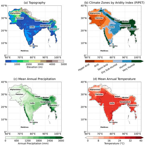
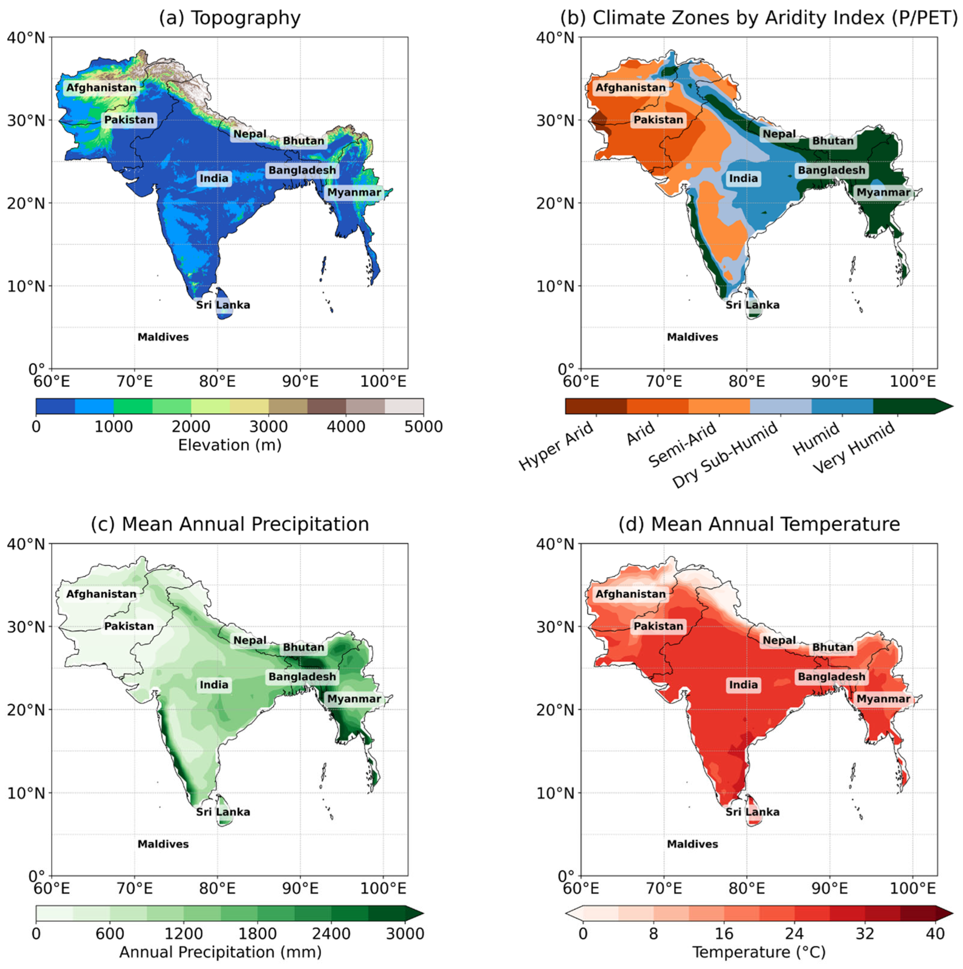
Figure 2. Spatial characteristics of the South Asian Monsoon region (Afghanistan, Bangladesh, Bhutan, India, Maldives, Myanmar, Nepal, Pakistan, and Sri Lanka) spanning 60–103° E longitude and 0–40° N latitude: (a) Topography (m), (b) climate classification by UNEP Aridity Index, (c) mean annual precipitation (mm) and (d) mean annual temperature (°C).

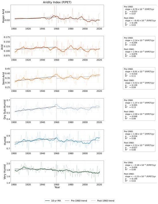
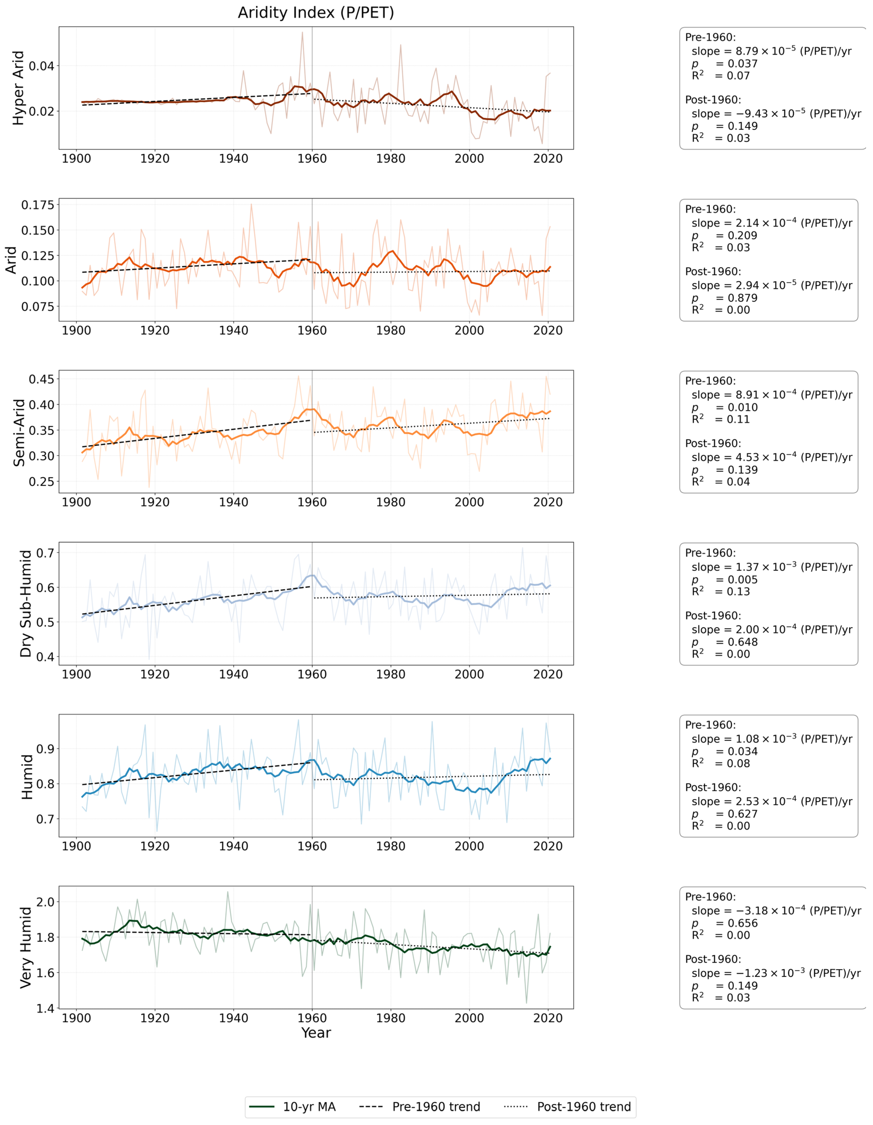
Figure 3. Time series (1901–2020) of mean annual Aridity Index across South Asian aridity zones, stratified according to the UNEP climate classification (as in Figure 2b). Thin lines represent annual values, while thick lines show 10-year moving averages. Dashed and dotted lines indicate linear trends for the pre-1960 and post-1960 periods, respectively. Boxes within each panel report the trend slope, coefficient of determination (R²), and statistical significance. All curves represent area-weighted averages of gridded data within each climate zone and line color are according to climate zone as in Figure 2b.

2.3. Interannual Ocean Teleconnections

Interannual ENSO events were identified using the Niño3.4 index, defined as the SST anomaly averaged over 170–120° W and 5° S–5° N. Following NOAA criteria, moderate events were defined by anomalies exceeding 0.5 °C, and strong events by anomalies exceeding 1.0 °C. Interannual IOD events were identified using the Dipole Mode Index (DMI), calculated as the difference in SST anomalies between the western Indian Ocean (50–70° E, 10° S–10° N) and the southeastern Indian Ocean (90–110° E, 10° S–0° N) [33]. Positive IOD events were defined by DMI values exceeding +0.4 °C, and Negative IOD events by values falling below −0.4 °C. ENSO-related SST variability was analyzed using Empirical Orthogonal Function (EOF) decomposition [34] applied to tropical Pacific SSTs (100° E–60° W, 30° S–30° N). EOF analysis employed cosine latitude weighting to account for varying grid-cell areas base on climatology of 1901–2024. The first three EOF modes were retained, explaining the dominant ENSO-related variance. To assess ENSO and IOD impacts on regional hydroclimate, composite anomalies of aridity during El Niño, La Niña, Positive IOD, and Negative IOD years were calculated. Spatial correlations between aridity and global SST anomalies were further computed across UNEP aridity zones.

2.4. Climate Variability Patterns of Aridity

EOF analysis was applied to Aridity Index, precipitation, temperature, and PET over 1901–2024. For SST, we computed SST composite EOFs for Pacific Region, which are distinct from the three leading EOF modes described earlier, using only strong ENSO years (5 El Niño and 6 La Niña events identified by a ±1.0 Niño-3.4 threshold). This approach follows common ENSO-composite EOF practice and allows us to isolate SST spatial patterns that are characteristic of extreme ENSO phases. Two-sample t-tests were used to assess statistically significant differences in the loading patterns.

2.5. Machine Learning Framework

To quantify the predictive skill of tropical oceanic signals on South Asian aridity, a benchmark multiple linear regression (LR) model was compared with a nonlinear Random Forest (RF) regression model [35]. The predictor set included the Niño3.4, Niño1+2, Niño3, and Niño4 indices, the IOD index, and their 2-year lagged anomalies, while the target variable was the regional UNEP Aridity Index over South Asia study domain. The RF model was configured with 500 decision trees, with the maximum tree depth optimized using 5-fold cross-validation. Model training was conducted over the period 1901–2000, and predictive performance was independently evaluated for 2001–2024.

2.6. Model Interpretation and Evaluation

To interpret model predictions and quantify driver contributions, we employed two complementary approaches: Variance Inflation Factor (VIF) for multicollinearity diagnostics and SHapley Additive exPlanations (SHAP) for feature attribution. Multicollinearity among predictors was assessed using the Variance Inflation Factor:

$${VIF}_j={\displaystyle \frac{1}{1-R_j^2}}$$

(5)

where $R_j^2$ is the coefficient of determination from regressing predictor j on all other predictors. VIF values exceeding 10 indicate severe multicollinearity that can destabilize coefficient estimates in linear models, while values between 5 and 10 suggest moderate correlation, and values below 5 are considered acceptable [36,37].

Feature importance for the RF model was assessed using Mean Decrease in Impurity (MDI) and SHAP values. The SHAP framework quantifies the marginal contribution of each feature to the model prediction:

$${\varnothing }_i= {\sum }_{S\subseteq F\left\{i\right\}}{\displaystyle \frac{\left|S\right|!\left(\left|F\right|-\left|S\right|-1\right)!}{\left|F\right|!}}[f(S\cup \left\{i\right\})-f\left(S\right)]$$

(6)

where |∅| is the SHAP value for feature ‘i’, ‘F’ is the full feature set, and f(S) is the model prediction using feature subset S.

Model skill was evaluated using the Temporal Correlation Coefficient (TCC) and the Mean Squared Skill Score (MSSS):

$$TCC={\displaystyle \frac{{\sigma }_{xy}}{{\sigma }_x{\sigma }_y}}$$

(7)

$$MSSS=1-{\displaystyle \frac{{MSE}_{model}}{{MSE}_{ref}}}$$

(8)

where σ_xy is the covariance between predicted and observed values, σ_x and σ_y are their standard deviations, and MSE denotes mean squared error.

3. Results

The South Asian Monsoon (SAM) region displayed marked spatial and temporal variability in hydroclimatic conditions, influenced by topography, atmospheric circulation, and oceanic modes such as ENSO and IOD. This section presents the key findings from analyses of historical climate data (1901–2024), including spatial patterns, trends, teleconnections, and machine learning predictions of aridity.

3.1. Spatiotemporal Hydroclimatic Patterns of the South Asian Monsoon Region

Pronounced geographic gradients govern the spatial distribution of moisture and energy across the region. Figure 2 presents the spatial distribution of key physiographic and hydroclimatic variables across the South Asian Monsoon region, including terrain elevation, Aridity Index, precipitation, and temperature. The spatial patterns revealed pronounced gradients largely controlled by topography and atmospheric circulation. Terrain elevation ranges from low-lying alluvial plains to heights exceeding 5000 m in the Himalayan arc (Figure 2a), where orographic lifting enhances precipitation on windward slopes while creating rain-shadow effects downstream. The UNEP Aridity Index (Figure 2b) reflects these topographic controls, transitioning sharply from hyper-arid conditions in southern Afghanistan and western Pakistan (AI < 0.05) to humid regimes in northeastern India, Bangladesh, and Myanmar (AI > 0.65). Annual precipitation (Figure 2c) follows this gradient, ranging from 400 to 600 mm yr⁻¹ in the arid northwest, increasing to 1000–1500 mm yr⁻¹ across central India, and exceeding 2500–3000 mm yr⁻¹ in the northeast. Mean annual temperature (Figure 2d) similarly mirrors elevation and aridity patterns, remaining below 10 °C in the high Himalayas, reaching 24–28 °C across lowlands, and rising to 30–32 °C within the driest zones.

Long-term trends differ systematically across aridity regimes as shown in (Figure 3). Figure 3 exhibits the time series of the Aridity Index, precipitation and temperature across the major aridity zones of South Asia for the period (1901–2020). Hyper-arid regions maintained persistently low AI (<0.05) and annual precipitation generally below 100 mm. Temperature records across all zones showed a gradual warming tendency after the mid-twentieth century, although the magnitude of the trend varies among climate regimes. The strongest warming occurs in the drier zones, while the humid and very humid zones exhibited more moderate temperature increases. Changes in Aridity Index also vary across regions: the hyper-arid zone showed the most evident post-1960 decline in AI, whereas semi-arid and dry sub-humid zones displayed interannual variability with weaker long-term trends. In the humid and very humid zones, slight increases in precipitation after the 1960s are accompanied by modest changes in Aridity Index, indicating the combined influence of precipitation variability and increasing evaporative demand.

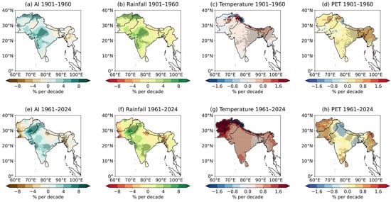
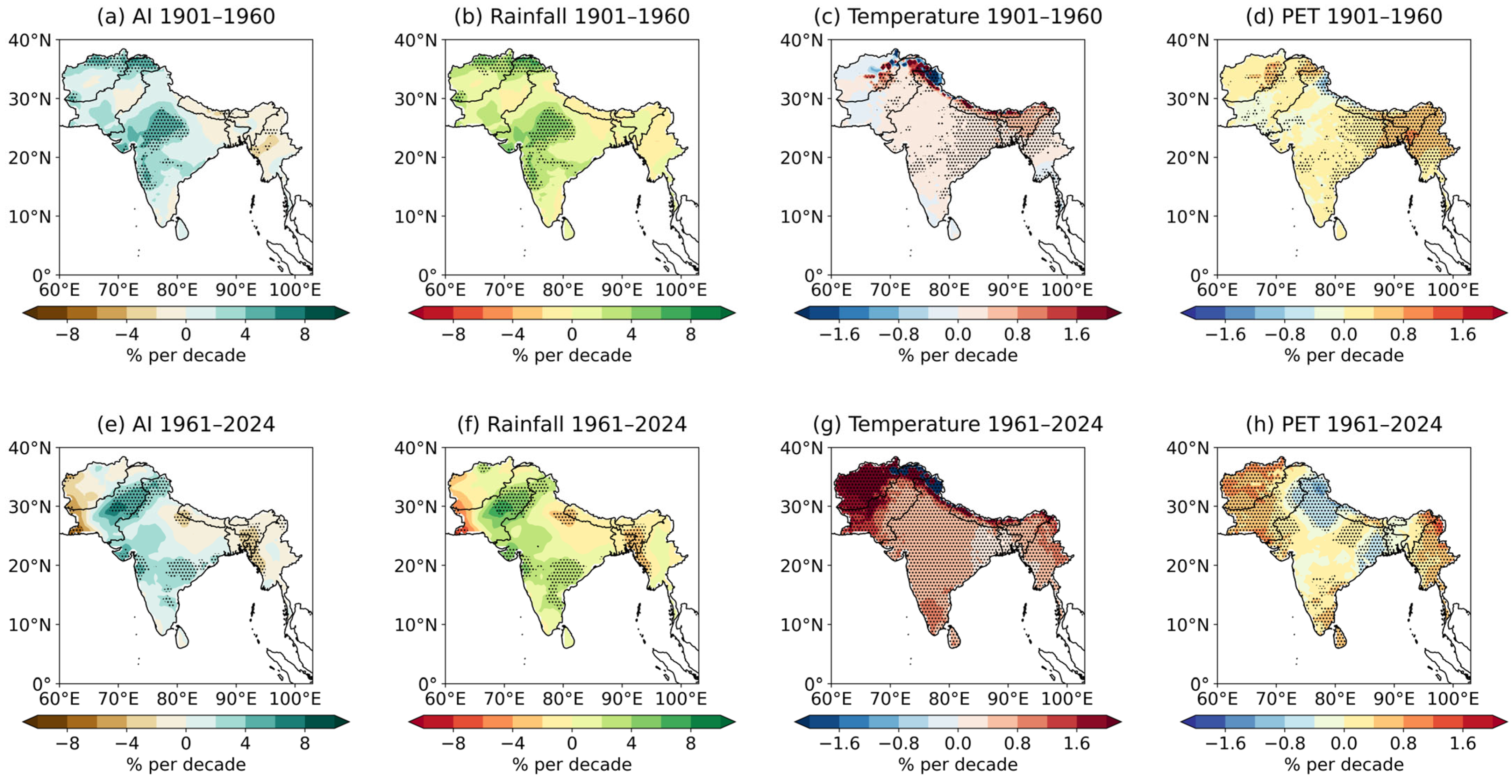
Moreover, the spatial grid point trends in the major hydroclimatic variables across the region from 1901 to 2020 at annual, decadal, and climatological scales is explained (Figure 4). The three trend estimates show broadly consistent spatial patterns, although the decadal smoothing highlights the most coherent regional signals. The Aridity Index exhibited significant drying in northwestern India and Pakistan, with declines of 6% to 8% per decade, while localized wetting trends of 2% to 4% per decade emerged in the northeastern region and along the Himalayan foothills. Corresponding precipitation trends revealed decreases of 4% to 6% per decade across the northwest but modest increases of 2 to 3% per decade in central and northeastern regions. Temperature trends showed widespread warming, strongest in northern Pakistan, Afghanistan, and the Himalayan belt (up to 1.6% per decade). PET increased by 0.8% to 1.6% per decade over central India and the Indo-Gangetic Basin reinforce growing evaporative pressures across much of the domain. Collectively, these findings demonstrate a century-long intensification of both thermal and evaporative stress across large parts of the SAM domain. Because these spatial and temporal trends reflect both local hydroclimatic forcing and remote climate variability, the following section investigates how large-scale oceanic modes, particularly ENSO modulate aridity across the region.

Figure 4. Spatial trends of climate variable (1901–2024) over South Asian Monsoon region, expressed as percentage change per decade: (a–d) Annual trends, (e–h) decadal (10-year) smoothed trends, and for (a,e) Aridity Index, (b,f) precipitation, (c,g) temperature, and (d,h) PET. Dotted hatched areas indicate statistically significant trends (p < 0.05).

3.2. Oceanic Variability and Teleconnection Controls on Regional Aridity

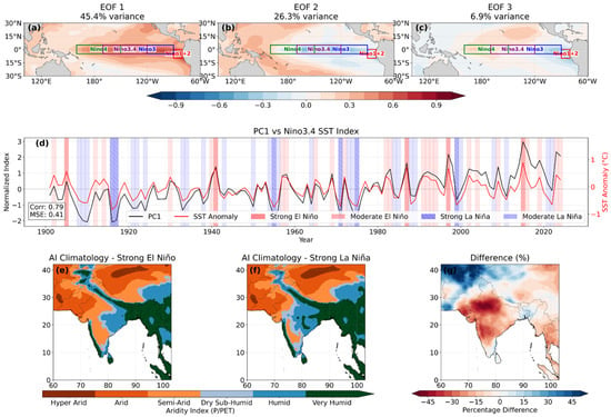
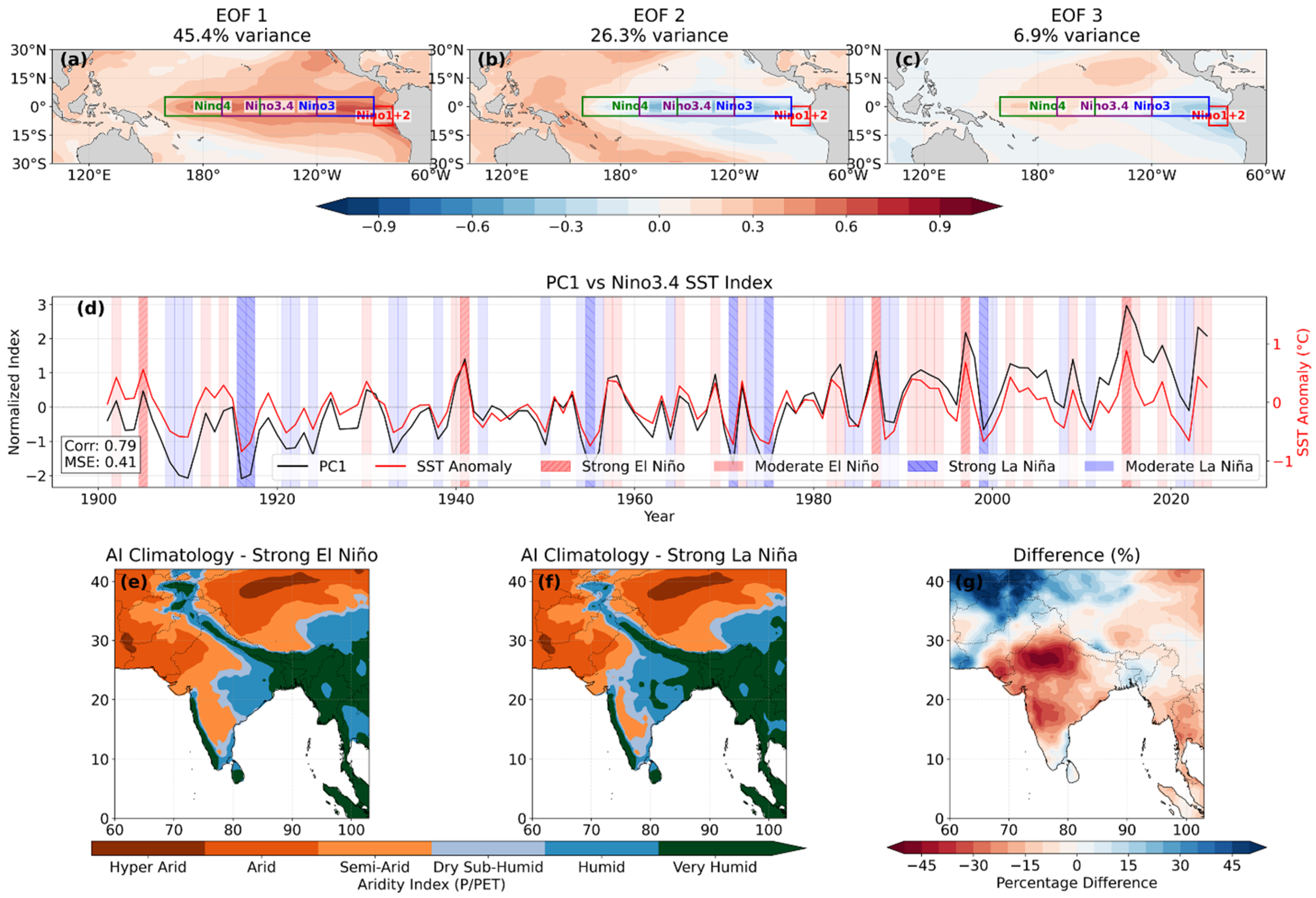
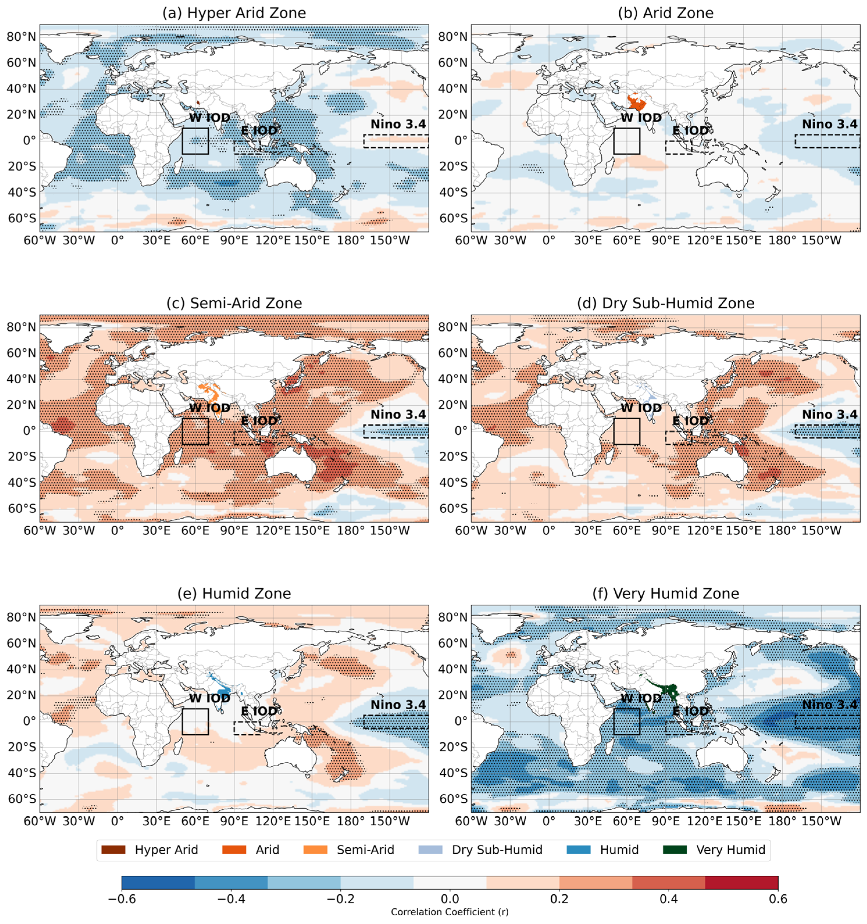
Large-scale ocean–atmosphere modes exerted considerable influence on aridity variability across the region (Figure 5, Figure 6, Figure 7 and Figure 8). EOF analysis of Pacific sea surface temperatures (SSTs; Figure 5a–c) identified three dominant modes: canonical ENSO centered in the eastern equatorial Pacific (EOF1; 45.4% variance), a Modoki-like pattern (EOF2; 26.3%), and secondary Pacific modes (EOF3; 6.9%). The first principal component (PC1) exhibited strong correlation with the Niño3.4 index (r = 0.79; Figure 5d), confirming ENSO as the dominant driver of regional hydroclimatic variability. Separate composite averaging were calculated for years when the Nino3.4 SST anomaly exceeded ±1.0 °C during 1901–2024 and we got strong El Niño (1905, 1941, 1987, 1997, 2015) and strong La Niña (1916, 1917, 1955, 1971, 1975, 1999) years. The composite analyses showed the contrasting impacts of ENSO phases on regional moisture availability. El Niño events substantially suppressed Aridity Index values across northwest and central India, reducing moisture availability to 60–70% of climatology, whereas La Niña conditions enhanced Aridity Index to 80–100% of normal across the Indo-Gangetic Plain and central India (Figure 5e,f). The El Niño minus La Niña difference patterns (Figure 5g) revealed dipole structures with AI reductions reaching 45% over the Indo-Gangetic Plain during El Niño, partially compensated by positive anomalies of 20–30% in the northeast during La Niña.

Figure 5. Pacific Ocean climate modes and their impacts on South Asian aridity: (a–c) First three EOFs of tropical Pacific (100° E–60° W, 30° S–30° N) SST (shaded) with Niño region boundaries (colored boxes); (d) normalized PC1 (black) and Niño3.4 SST anomaly (red) time series (1901–2024) with ENSO events highlighted (moderate: solid fill, strong: hatched); (e,f) Composite Aridity Index (P/PET) during (e) strong El Niño and (f) strong La Niña years classified by UNEP climate zones; (g) percentage difference in Aridity Index between strong El Niño and La Niña composites. EOF analysis used cosine latitude weighting, and ENSO events were defined using ±0.5 °C (moderate) and ±1.0 °C (strong) Niño3.4 SST anomaly thresholds.

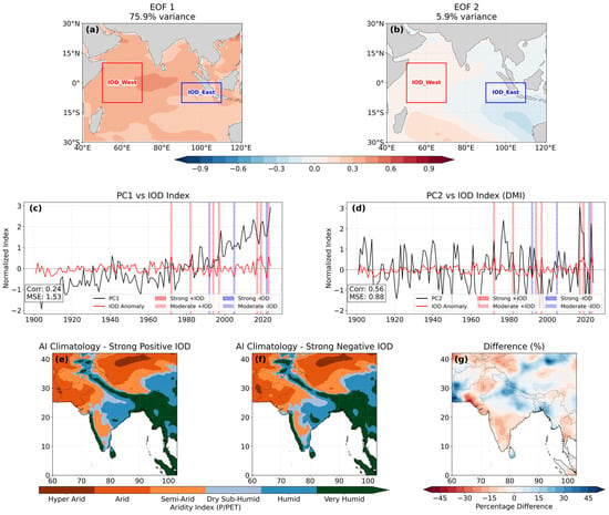
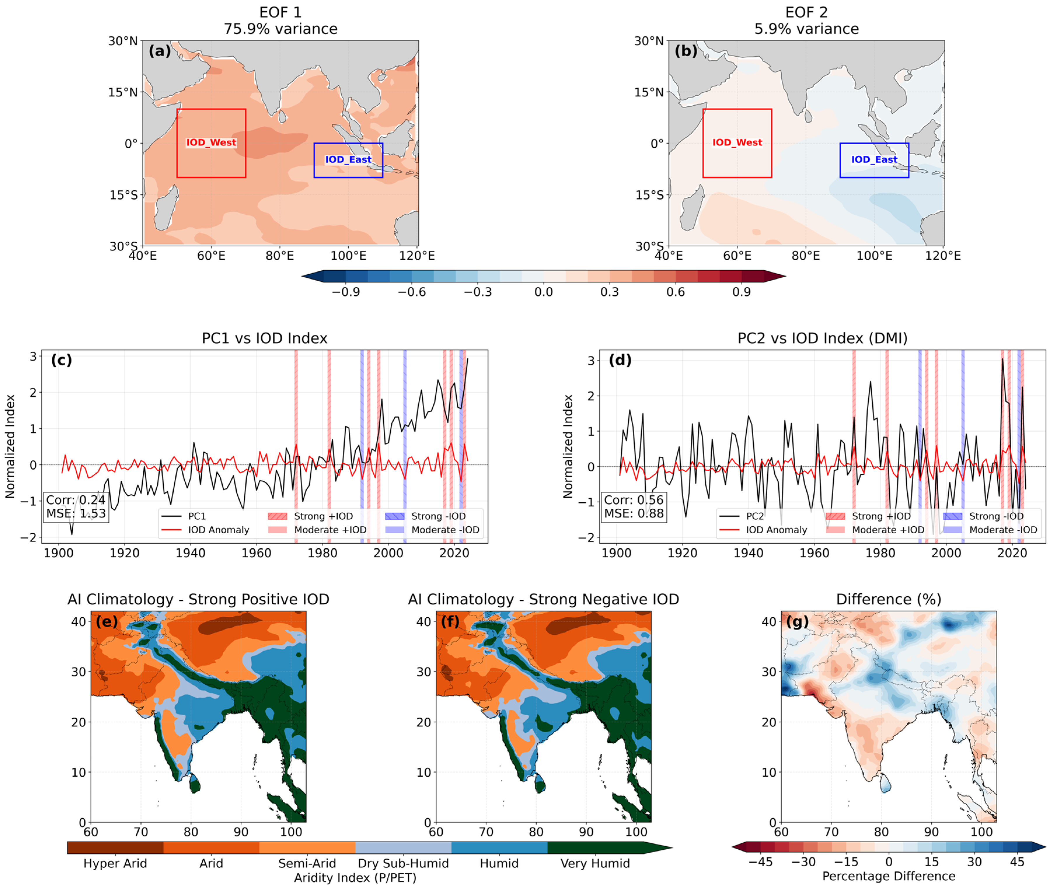
Figure 6. Indian Ocean Dipole and its impacts on South Asian aridity: (a,b) First two EOFs of tropical Indian Ocean (40–120° E, 30° S–30° N) SST (shaded) with the western (50–70° E, 10° S–10° N) and eastern (90–110° E, 10° S–0° N) IOD poles (colored boxes); (c,d) normalized PCs (black) and Dipole Mode Index (DMI) SST anomaly (red) time series (1901–2024) with IOD events highlighted (moderate: solid fill, strong: hatched); (e,f) Composite Aridity Index during (e) strong positive IOD and (f) strong negative IOD years classified by UNEP climate zones; (g) percentage difference in AI between strong positive and negative IOD composites. EOF analysis used cosine latitude weighting, and IOD events were defined using ±0.5 °C (moderate) and ±1.0 °C (strong) DMI thresholds.

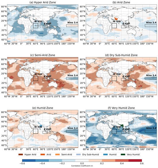
Figure 7. Spatial correlations (1901–2024) between South Asian aridity and global sea surface temperatures (SSTs), by UNEP climate zones: (a) hyper-arid, (b) arid, (c) semi-arid, (d) dry sub-humid, (e) humid, and (f) very humid zones. Dotted hatching denotes statistically significant correlations (p < 0.05). Black boxes highlight Niño3.4 (170–120° W, 5° S–5° N; dashed) and Indian Ocean Dipole (50–70° E, 10° S–10° N; solid) regions.

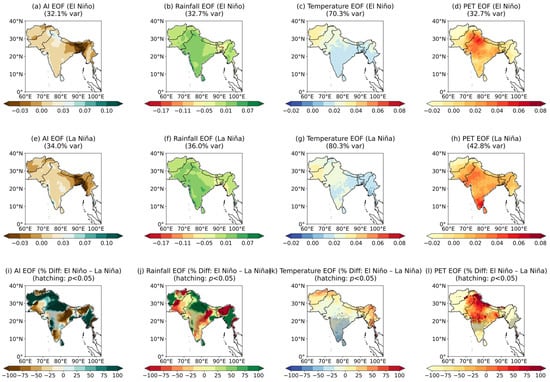
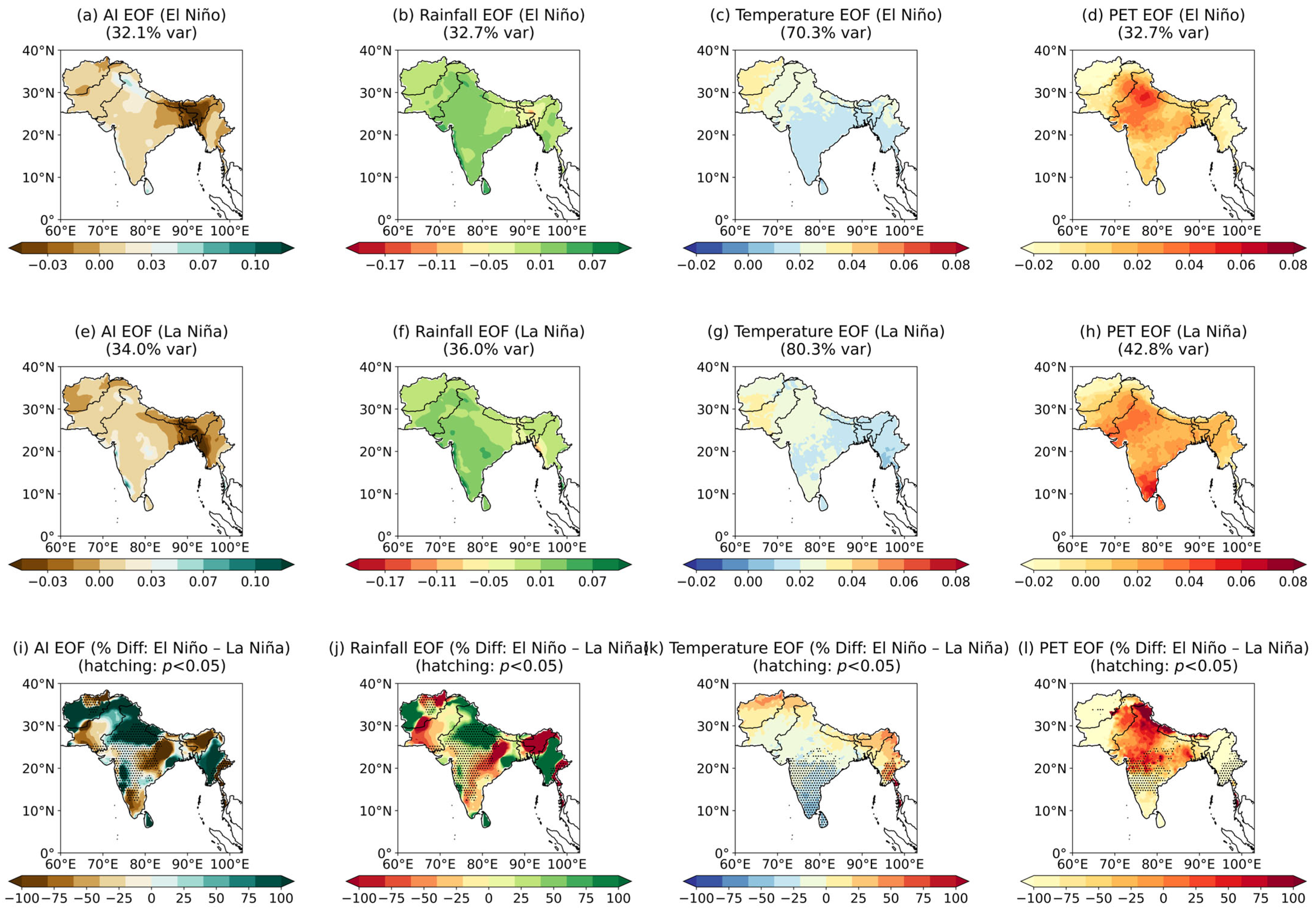
Figure 8. Dominant climate variability patterns during strong ENSO events (ENSO extremes) over South Asia (1901–2024): (a–d) First EOF modes of (a) Aridity Index (AI), (b) precipitation, (c) temperature, and (d) potential evapotranspiration (PET) during strong El Niño years; (e–h) corresponding EOF patterns during strong La Niña years; (i–l) percentage differences between El Niño and La Niña EOF patterns (hatching indicates p < 0.05 significance from two-sample t-test. Strong ENSO events were defined using historical thresholds (±1.0 °C Niño3.4 SST anomaly).

In addition to Pacific variability, the IOD also contributes to hydroclimatic variability across South Asia (Figure 6). The EOF analysis of tropical Indian Ocean SST reveals a basin mode (IOB, Figure 6a) and a dipole mode (IOD, Figure 6b). The leading principal component (PC1) showed a long-term trend, consistent with previous reports of tropical SST warming [38]. The time series of PC2 is consistent with the Dipole Mode Index (DMI), capturing major IOD events from 1990 to 2024 (Figure 6d). Composite analyses illustrate the contrasting hydroclimatic impacts of IOD phases. Strong positive IOD events generally correspond to enhanced Aridity Index values across parts of South Asia, indicating relatively wetter conditions, whereas negative IOD phases are associated with reduced Aridity Index and comparatively drier conditions (Figure 6e,f). The difference between positive and negative IOD composites (Figure 6g) highlights spatial contrasts in moisture response, demonstrating that Indian Ocean variability can modulate regional aridity patterns alongside Pacific-driven ENSO forcing.

Correlations between zone-specific Aridity Index and global sea surface temperatures revealed heterogeneous teleconnection sensitivities across the region (Figure 7a–f). Hyper-arid regions showed weak but slightly positive correlations with SST anomalies in the Niño3.4 region, whereas arid regions exhibited weak negative correlations, indicating that ENSO influences vary across the driest climate regimes. In contrast, semi-arid and dry sub-humid zones displayed stronger positive correlations with equatorial Pacific and Indian Ocean SSTs, suggesting greater hydroclimatic responsiveness to basin-scale ocean variability. Humid regions exhibited weaker and more spatially heterogeneous correlations, while very humid zones showed clearer negative correlations with equatorial Pacific SSTs, reflecting more complex interactions between ENSO variability and monsoonal circulation in the wettest parts of the domain.

EOF analysis of the hydroclimatic anomalies during strong ENSO phases (Figure 8a–i) further demonstrated ENSO-driven reorganization of regional water and energy fluxes. During El Niño, the leading Aridity Index mode (32.1% variance) reflects widespread drying across northwest and central regions, coinciding with reduced precipitation (32.7%) and sharply elevated PET (temperature-related variance: 70.3%). Conversely, La Niña produces a strongly coherent wetting mode (34.0%) linked to enhanced precipitation (36.0%) and reduced PET/cooling (80.3%). The resulting difference fields (Figure 8i–l) highlights distinct dipole structures, particularly the strong Aridity Index drying over the Indo-Gangetic Plain under El Niño and the thermal intensification across the Himalayas. Supplementary analyses (Figures S1–S6) verify the strength of these findings, including cross-index comparisons (UNEP vs. De Martonne), additional EOFs for individual hydroclimatic variables, and singular value decomposition (SVD) patterns linking SST variability with regional aridity.

3.3. Machine Learning Prediction of Aridity and Model Performance

To evaluate the predictive potential of tropical ocean variability for South Asian aridity, we developed machine learning and statistical modeling frameworks using the Niño3.4, Niño1+2, Niño3, and Niño4 indices, the IOD index, and their 1- and 2-year lagged anomalies as predictors. These indices capture the persistence and multi-year teleconnections of oceanic modes that modulate monsoon behavior and hydroclimatic variability across the subcontinent. Random Forest (RF), configured as an ensemble of 500 trees with maximum depth optimized via 5-fold cross-validation on the training data, serves as a nonlinear benchmark. Linear Regression (LR) provides a baseline representing additive, linear responses. We additionally developed a Hybrid model that combines RF predictions with the LR framework by using RF output as an additional predictor, integrating nonlinear feature extraction with linear interpretability. Model skill was evaluated using the Mean Squared Skill Score (MSSS) against a climatology reference forecast and the Temporal Correlation Coefficient (TCC). All hyperparameters were determined exclusively on the training period (1901–2000), ensuring no information from the validation era (2001–2024) influenced model configuration. We first examine the mechanistic basis for model predictions through interpretability analysis (Section 3.3.1), focusing on feature importance and nonlinear predictor–response relationships over the full historical period (1901–2024). This is followed by comprehensive temporal and spatial validation over the independent hold-out period (Section 3.3.2).

3.3.1. Model Interpretation and Climate Driver Attribution

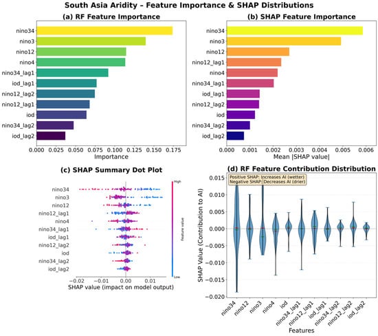
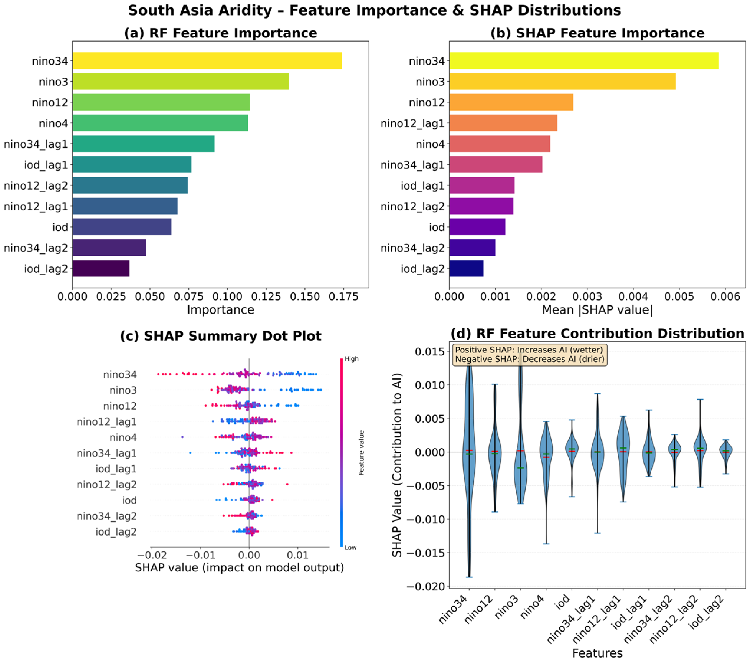
To explain the predictive mechanisms underlying model performance, we conducted a comparative interpretability analysis of the RF and LR models (Figure 9 and Figure S11). Feature importance was quantified using both standard RF Mean Decrease in Impurity (MDI; Figure 9a) and SHapley Additive exPlanations (SHAP) values (Figure 9b and Figure S7 in the Supplementary Materials). SHAP provides more reliable attribution than MDI alone by decomposing predictions into additive contributions from each predictor. Both methods identified Niño3.4 as the dominant predictor, followed by Niño3 and Niño1+2, confirming ENSO variability as the primary source of predictable aridity variance. One-year lagged ENSO indices (Niño3.4_lag1, Niño1+2_lag1) ranked as secondary predictors, while IOD-related variables (IOD, IOD_lag1) showed moderate but consistent importance, indicating that Indian Ocean variability modulates but does not override ENSO-driven impacts.

Figure 9. Machine learning analysis of South Asian aridity. (a) Standard Random Forest feature importance. (b) SHAP-based feature importance. (c) SHAP value distribution (red = high feature values, blue = low). (d) RF feature contribution distribution.

Prior to interpretability analysis, we assessed multicollinearity among predictors using the Variance Inflation Factor (VIF). Severe multicollinearity can inflate regression coefficients and impair interpretability in linear models. VIF analysis (Figure 9c and Figure S8) revealed that simultaneous ENSO indices (Niño3.4, Niño3, Niño1+2, Niño4) displayed severe multicollinearity (VIF > 10; range: 15.47–103.16), as expected given their physical interdependence. Lagged ENSO indices (Niño3.4_lag1–2, Niño1+2_lag1–2) and IOD-related variables, however, showed acceptable multicollinearity (VIF < 5), indicating that temporal separation effectively reduces predictor redundancy. These findings justify the inclusion of multiple ENSO indices in the RF model, which is robust to multicollinearity in prediction, while cautioning against overinterpreting individual LR coefficients. We note that high multicollinearity among simultaneous Niño-region indices may introduce instability into SHAP attributions; the reported feature rankings should therefore be interpreted as indicative rather than definitive.

The SHAP value distributions (Figure 9c) revealed pronounced asymmetries in predictor–response relationships. For Nino3.4, high index values (red points, indicating El Nino conditions) consistently shifted predictions toward higher aridity (positive SHAP values), while low values (blue points, La Nina conditions) reduced aridity predictions (negative SHAP values). Critically, the distribution showed asymmetric spread: extreme positive Nino3.4 values produced disproportionately large positive SHAP contributions compared to the negative contributions from equivalent-magnitude La Nina events, indicating threshold-dependent responses. Similar but weaker asymmetries appeared for Nino3 and Nino12. In contrast, IOD indices displayed more proportional, bidirectional influences with substantial overlap between positive and negative values, suggesting complex conditional effects that depend on the concurrent ENSO state.

Individual prediction explanations for extreme years illustrated the compound nature of aridity drivers. For the wettest year of the record, 1959 (AI = 0.737; Figure S11), positive SHAP contributions from lagged La Niña-like indices (low Niño3.4, low Niño3) dominated the prediction, collectively pushing the model toward extreme wetness. IOD-related variables provided smaller offsetting contributions, partially mitigating but not reversing the strong ENSO-driven wetting signal. Conversely, for the driest year, 1972 (AI = 0.589; Figure S11), negative SHAP contributions from El Niño-like conditions (high Niño3.4_lag1, high Niño1+2) drove predictions toward increased aridity (i.e., a decreased Aridity Index), with IOD contributions again providing secondary modulation. These results demonstrate that extreme aridity anomalies result from aligned contributions across multiple ENSO indices rather than single-predictor dominance, with IOD effects modulating the magnitude but rarely reversing the ENSO-driven tendency.

A comparison of time series showed the model prediction skill over the full 1901–2024 period (Figure S11). The RF model (red dashed line) closely tracked observed aridity variability (black line), capturing both interannual fluctuations and extreme events with high fidelity (MSE: 0.0003; TCC: 0.656; MSSS: 0.701 for 1901–2000). The LR model (blue dotted line) reproduced the general temporal patterns but systematically underestimated peak amplitudes and failed to capture the sharp transitions evident in 1959, 1972, and other extreme years, resulting in degraded performance (MSE: 0.0006; TCC: 0.566; MSSS: 0.320 for 1901–2000). The RF model’s superior reconstruction of extreme events reflects its capacity to capture the nonlinear, threshold-dependent ENSO responses and compound multi-predictor effects revealed in the SHAP analysis, which the additive linear framework cannot represent.

3.3.2. Comparative Temporal and Spatial Validation of RF and LR Models

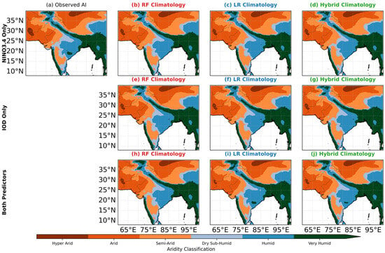
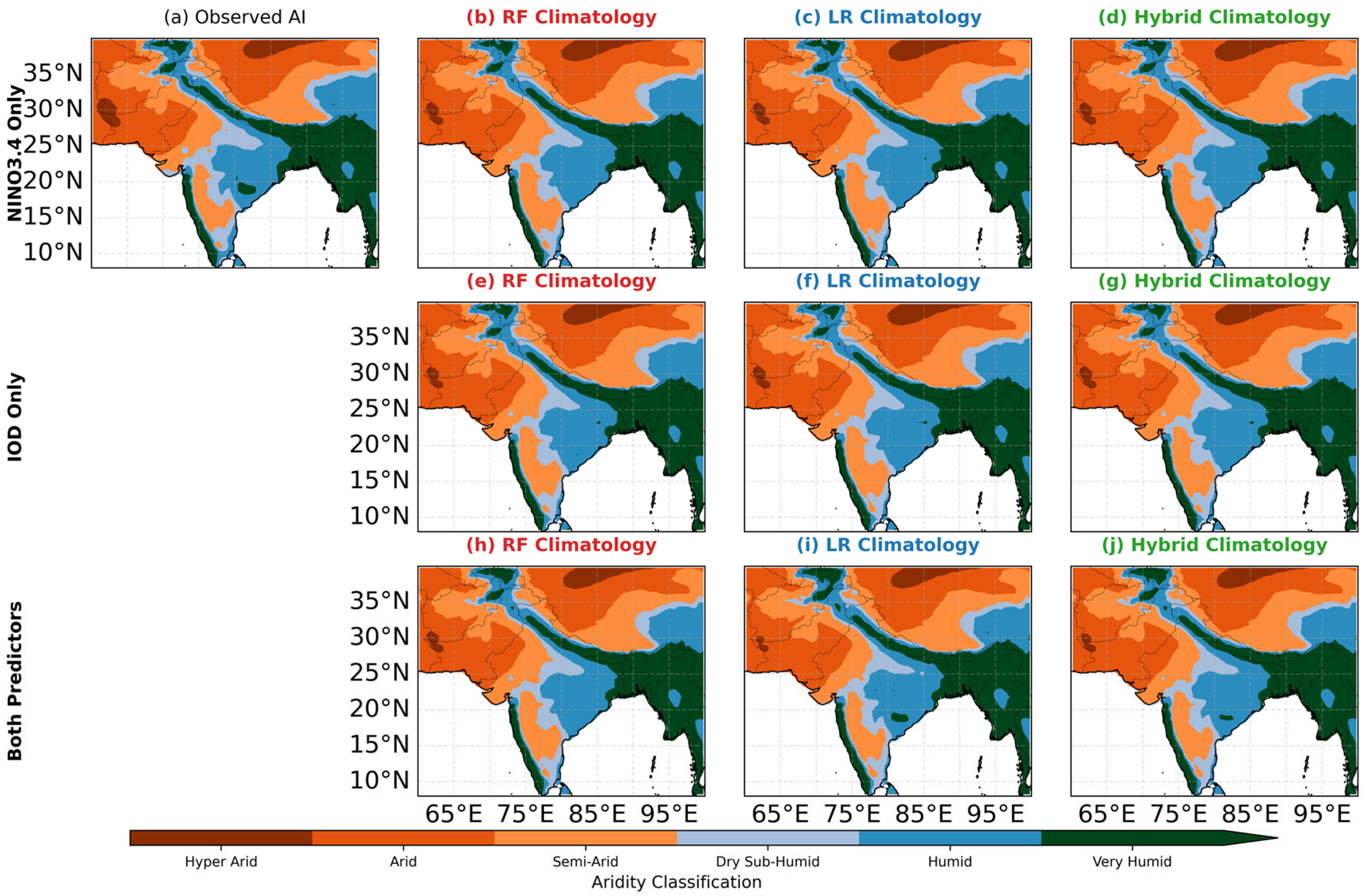
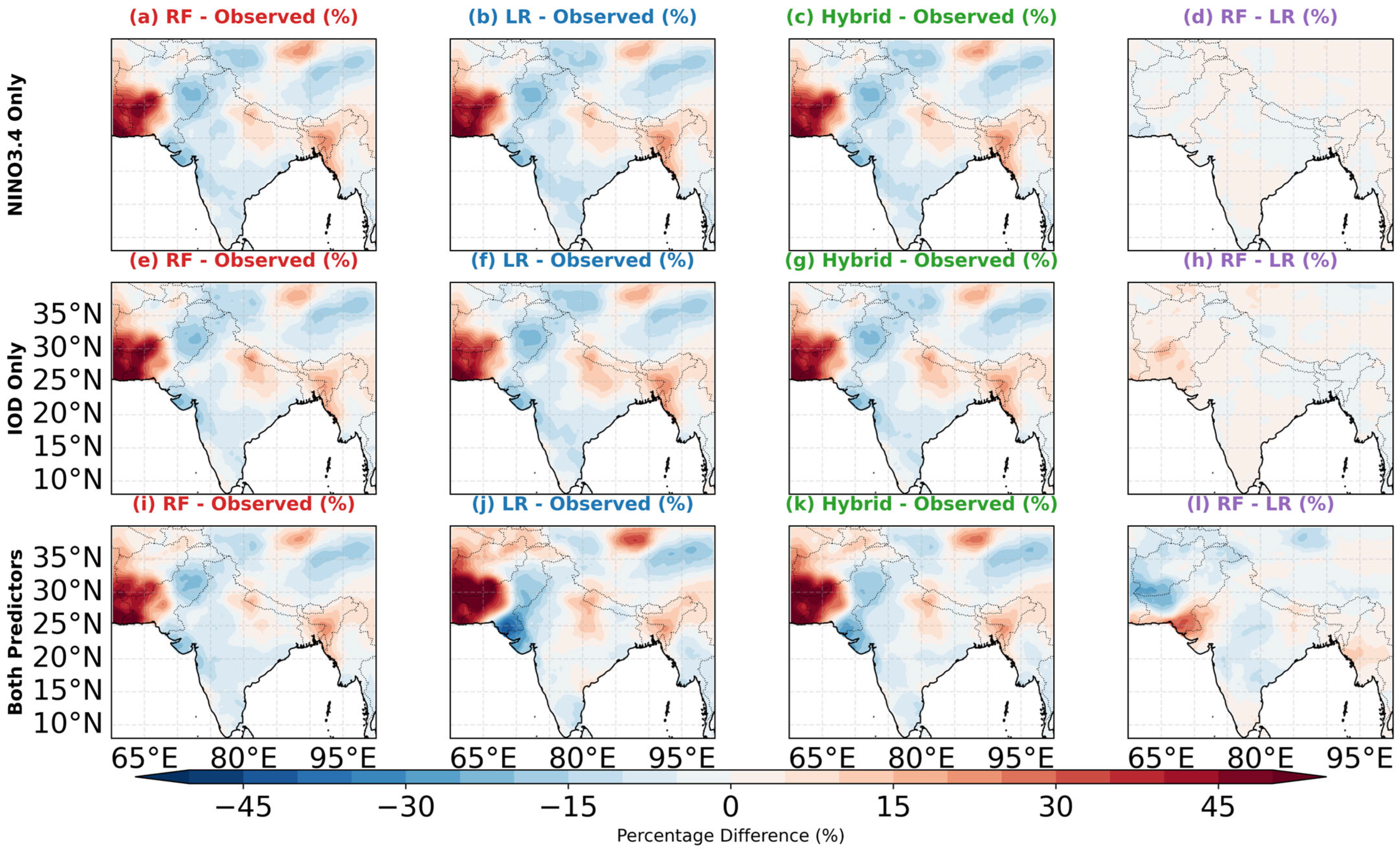
Building on the mechanistic insights from the interpretability analysis, we conducted a comprehensive evaluation of RF and LR model performance during the independent validation period (2001–2024). Figure 10 provides a spatially explicit comparison of observed aridity climatology and model predictive skill across the region. The observed Aridity Index climatology (Figure 10a) exhibited pronounced spatial gradients from hyper-arid zones in the northwest (Afghanistan, Pakistan) to humid regions in the east (Myanmar, northeastern India). The RF model’s mean Aridity Index prediction (Figure 10b) successfully captured this spatial structure with minimal systematic bias (Figure 11a,d,g), demonstrating its capability to reproduce regional-scale moisture gradients for independent validation period. In contrast, the LR model’s mean Aridity Index prediction (Figure 10c) captured the broad regional structure but exhibited notable systematic biases: overestimation in the Indo-Gangetic Plain and significant underrepresentation of aridity in the arid northwest (Figure 11b,e,h). These climatological biases are consistent with the LR model’s intrinsic limitation in accounting for the physically significant nonlinearities and complex teleconnection interactions identified.

Figure 10. Spatial distribution of aridity index (AI) climatology for the period 2001–2024 across South Asia for different predictor combinations. (a) Observed AI climatology derived from CRU precipitation (P) and potential evapotranspiration (PET) data (AI = P/PET). (b–d) AI climatology predicted by random forest (RF), linear regression (LR), and hybrid (RF + LR)/2 models using only NINO3.4 sea surface temperature indices and their lags. (e–g) Same as (b–d) but using only Indian Ocean Dipole (IOD) indices. (h–j) Same as (b–d) but using both NINO3.4 and IOD indices. Aridity classification follows the UNEP aridity categories: hyper-arid (<0.03), arid (0.03–0.20), semi-arid (0.20–0.50), dry sub-humid (0.50–0.65), humid (0.65–1.0), and very humid (>1.0). Models were trained on data from 1901 to 2000 and validated over the 2001–2024 period.

Figure 11. Percentage differences between predicted and observed AI climatology (2001–2024) across South Asia for different predictor combinations. (a–c) RF, LR, and hybrid model differences using NINO3.4 indices only. (e–g) Same as (a–c) but using IOD indices only. (i–k) Same as (a–c) but using both NINO3.4 and IOD indices. (d,h,l) RF minus LR percentage differences for the three predictor sets, highlighting systematic differences between machine learning and linear regression approaches. Positive values (red shades) indicate overestimation, while negative values (blue shades) indicate underestimation relative to observations. For panels (d,h,l), positive values indicate RF predicts a higher Aridity Index (i.e., wetter conditions) than LR, and vice versa. White areas represent differences near zero (±5%). Percentage difference calculated as [(Predicted − Observed)/Observed] × 100% for (a–c,e–g,i–k) and [(RF − LR)/Observed] × 100% for (d,h,l). Models trained on 1901–2000, evaluated on 2001–2024.

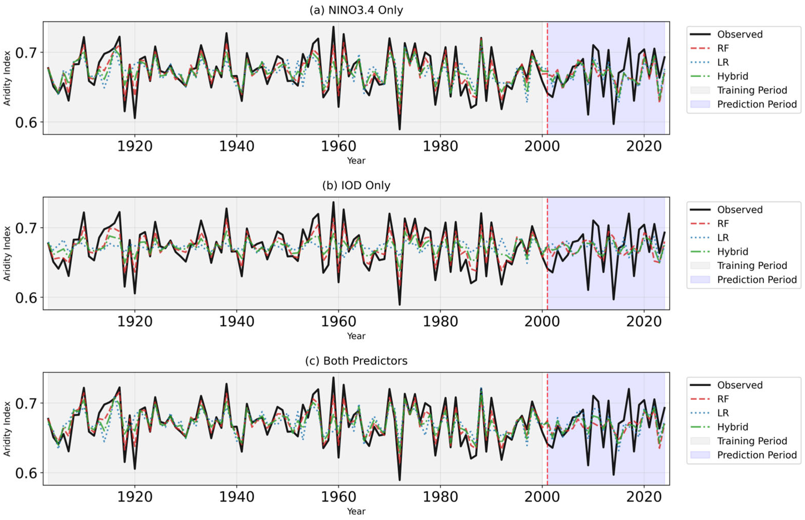
Assessment of interannual variability during 2001–2024 further demonstrated model performance in capturing year-to-year fluctuations. Domain-averaged time series (Figure 12a–c) showed that all three models tracked the general temporal evolution of Aridity Index. Comparison against simple benchmarks (Figure S7) confirms that these high skill scores reflect genuine predictive capability rather than fortuitous persistence or long-term trends; a climatology reference achieves near-zero skill, while a persistence forecast performs worse than the ML output. The Hybrid model’s superior aggregate performance stems from its ability to leverage both the nonlinear feature extraction of RF and the linear additive structure of LR, effectively capturing threshold-dependent ENSO responses alongside systematic linear trends. Visual inspection revealed that both RF and Hybrid models more consistently captured the magnitude of extreme dry and wet events, whereas the LR model tended to dampen extremes a pattern consistent with the nonlinear threshold responses identified in the SHAP analysis.

Figure 12. Temporal evolution of area-averaged Aridity Index over South Asia for different predictor combinations. (a) Time series using only NINO3.4 indices, (b) using only IOD indices, and (c) using both predictors. Black solid line represents observed AI, while dashed red, dotted blue, and dash-dot green lines represent RF, LR, and hybrid model predictions, respectively. Gray shading indicates training period (1901–2000), blue shading indicates independent validation period (2001–2024), and red dashed vertical line marks the transition year (2001). All models capture the interannual variability but differ in their ability to reproduce extreme events and long-term trends.

Regional analysis further differentiated model behavior. The RF model exhibited notable performance advantages in areas where nonlinear ENSO–IOD controls are physically dominant, including Afghanistan, Pakistan, Myanmar, and the Maldives. Conversely, the LR model performed comparably or slightly better only in restricted regions such as Nepal, Bhutan, and Bangladesh, where local hydroclimate noise or weaker teleconnection signals may limit the benefit of RF complexity. Taken together, the spatial and temporal validation results underscore the advantage of the RF framework in representing tropical-ocean-driven aridity variability across diverse South Asian climatic regimes, particularly for long-term trends and spatial gradients. These outcomes build on the nonlinear and interactive mechanisms identified above and establish a foundation for exploring the broader utility of machine learning techniques in tropical climate prediction.

3.3.3. Influence of Long-Term Trends and Interannual Teleconnections

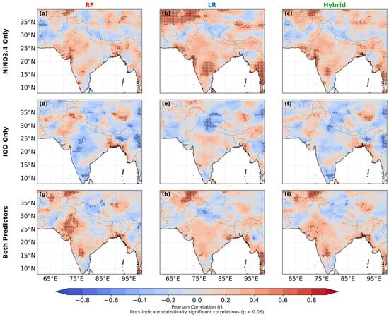
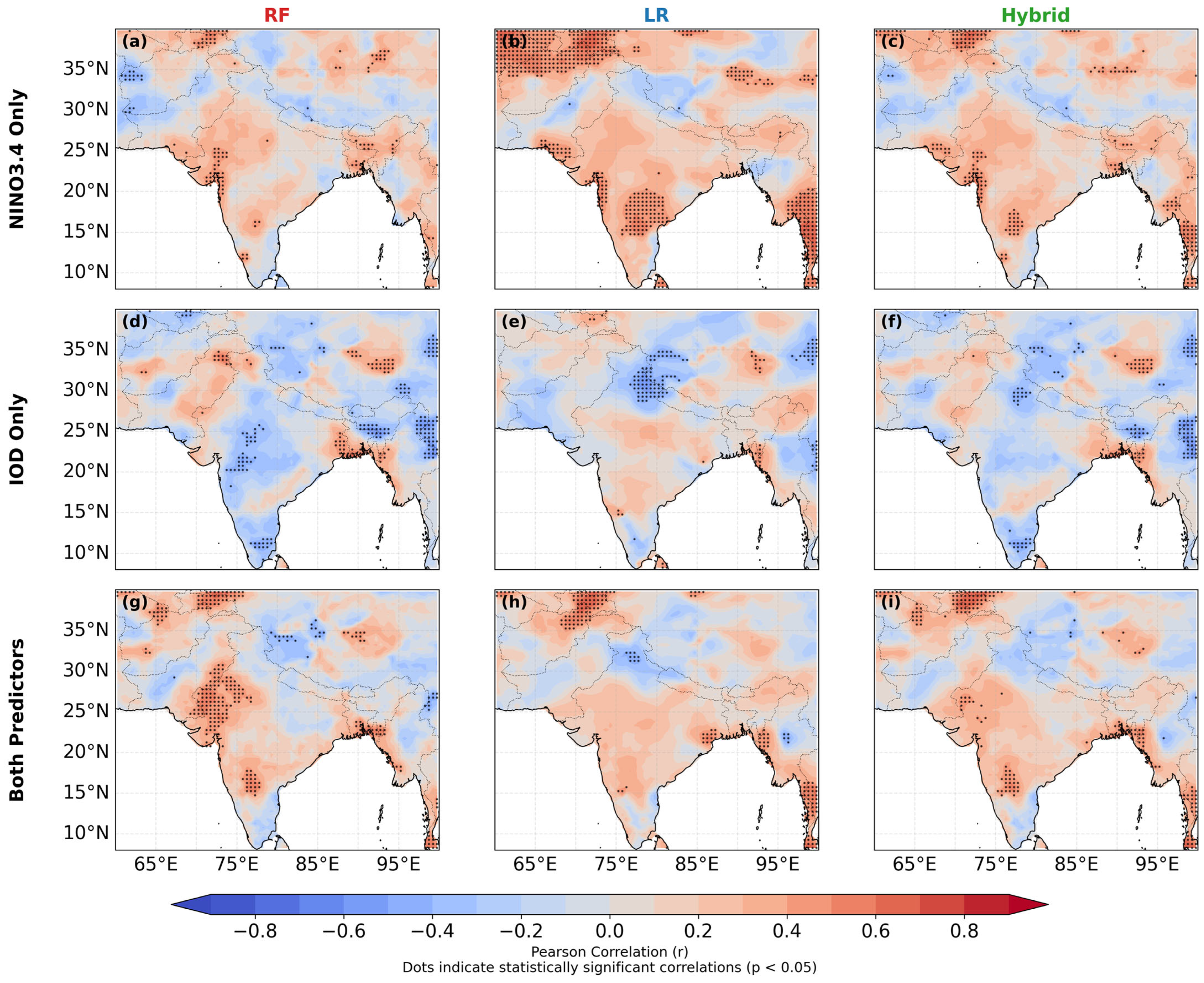
To assess whether the high predictive skill of the original models (R² for the area-averaged series) merely reflects long-term trends rather than genuine year-to-year teleconnections, we repeated the entire modeling procedure after linearly detrending both the target Aridity Index and all predictor indices. Detrending was performed per grid cell (for AI) and per index over the full 1901–2024 period, removing any linear trend and leaving only interannual anomalies. Figure 13 shows the Pearson correlation between detrended observed and predicted AI for the three predictor sets (Niño3.4 only, IOD only, and both). While the combined predictor set yielded positive correlations over most of South Asia, the magnitudes are modest (typically r < 0.5), indicating that the models capture only a fraction of the interannual variability. The highest correlations are found over northwestern India and parts of Pakistan, where ENSO and IOD teleconnections are known to be strongest. This visual impression is confirmed by the quantitative metrics summarized in Table 1 and Figure 14.

Figure 13. Spatial distribution of temporal Pearson correlation (r) between predicted and observed aridity index (AI) over South Asia for the period 2001–2024. Correlations are computed at each grid cell between detrended model predictions and CRU-derived observed AI. Rows correspond to predictor sets: (a–c) NINO3.4 indices only; (d–f) Indian Ocean Dipole (IOD) indices only; (g–i) both NINO3.4 and IOD indices. Columns correspond to models: random forest (RF; left), linear regression (LR; middle), and hybrid (RF + LR)/2 (right). Dots indicate statistically significant correlations (p < 0.05). Models were trained on 1901–2000 data and validated over the 2001–2024 period.

Table 1. Inter-model performance sensitivity test.

Zone	Model	R2 (Orig)	R2 (Det)	TCC (Orig)	TCC (Det)	RMSE (Orig)	RMSE (Det)	Bias (Orig)	Bias (Det)
Hyper-Arid	RF	0.668	0.728	0.873	0.898	0.001	0.001	0.000	0.000
	LR	0.029	0.082	0.272	0.311	0.001	0.001	0.000	0.000
	Hybrid	0.736	0.815	0.878	0.911	0.001	0.001	0.000	0.000
Arid	RF	0.563	0.658	0.774	0.845	0.005	0.004	0.001	0.001
	LR	0.022	0.088	0.295	0.331	0.007	0.007	0.001	0.001
	Hybrid	0.551	0.702	0.784	0.850	0.005	0.004	0.001	0.001
Semi-Arid	RF	0.593	0.643	0.808	0.848	0.008	0.008	0.002	0.002
	LR	0.008	0.085	0.246	0.310	0.013	0.013	0.002	0.001
	Hybrid	0.620	0.700	0.812	0.848	0.008	0.007	0.002	0.002
Dry Sub-Humid	RF	0.560	0.575	0.785	0.803	0.012	0.012	0.003	0.003
	LR	−0.108	0.108	0.166	0.353	0.019	0.017	0.004	0.002
	Hybrid	0.572	0.574	0.796	0.798	0.012	0.012	0.004	0.004
Humid	RF	0.543	0.530	0.771	0.771	0.015	0.015	0.004	0.004
	LR	−0.113	0.104	0.161	0.342	0.023	0.021	0.005	0.002
	Hybrid	0.609	0.527	0.803	0.766	0.014	0.015	0.003	0.004
Very Humid	RF	0.681	0.655	0.867	0.837	0.021	0.019	−0.004	0.003
	LR	0.246	0.301	0.498	0.552	0.032	0.027	−0.002	0.001
	Hybrid	0.747	0.691	0.870	0.839	0.019	0.018	−0.003	0.003

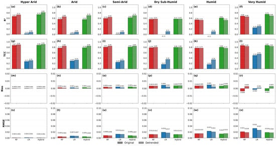
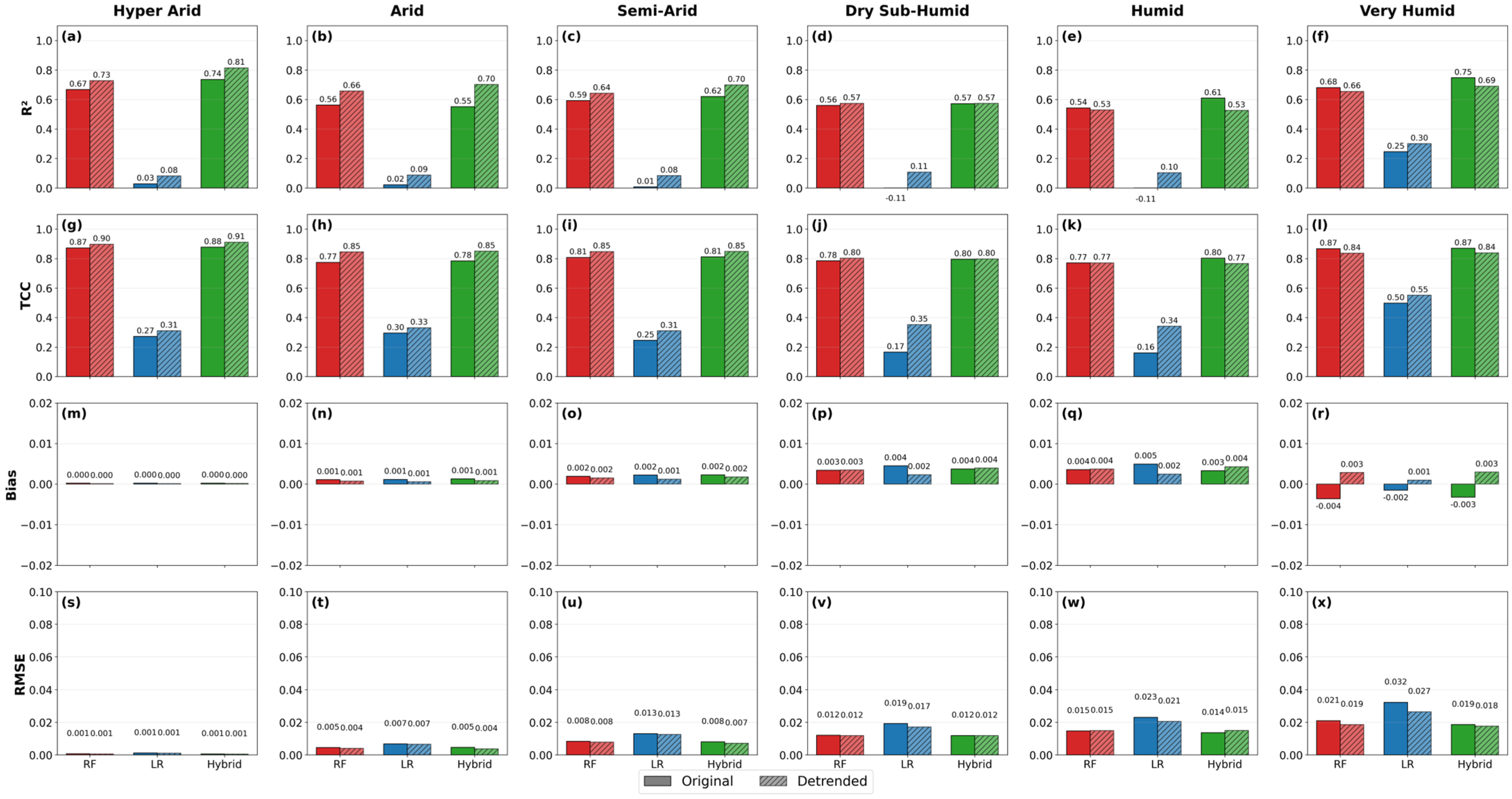
Figure 14. Model performance comparison by aridity zone for original versus detrended predictors across different methods. The 4 × 6 grid displays, from top to bottom, four evaluation metrics: (a–f) coefficient of determination (R²), (g–l) temporal correlation coefficient (TCC), (m–r) bias, and (s–x) root mean square error (RMSE). Columns represent the six UNEP aridity zones: hyper-arid, arid, semi-arid, dry sub-humid, humid, and very humid. Within each panel, solid bars show results using original predictors and hatched bars show results using detrended predictors, for Random Forest (RF, red), Linear Regression (LR, blue), and Hybrid (RF + LR)/2 (green) models. The zone-specific breakdown highlights the spatial heterogeneity of predictive skill across South Asia, revealing that area-averaged metrics mask contrasting regional responses.

When evaluated over the full domain, the original models achieve high skill (e.g., RF: R² = 0.72, TCC = 0.87), largely because they capture the strong long-term trend in aridity. However, the zone-specific breakdown (Table 1 and Figure 14) reveals significant spatial heterogeneity. The from 1901–2model performs exceptionally well in the hyper-arid (R² = 0.736) and very humid (R² = 0.747) zones, while the Linear Regression model produces negative R² values in the dry sub-humid and humid zones (R² < 0), indicating complete failure in these regions. After detrending, the area-averaged skill drops substantially (RF: R² = 0.20, TCC = 0.45), but the zone-specific detrended skill actually increases in the hyper-arid zone (Hybrid R² = 0.815), confirming that the trend is the dominant source of area-averaged predictive power while masking zone-specific interannual predictability. The linear regression model, which originally performed poorly in the area average (R² = 0.32), exhibits highly variable zone-specific skill. It fails completely in the humid and dry sub-humid zones under original predictors but improves slightly in the hyper-arid zone after detrending (R² increases from 0.029 to 0.082). This suggests that its modest area-averaged skill derives almost entirely from interannual covariation rather than long-term trends. The Hybrid model, while still outperforming the individual models in the area-averaged detrended case (R² = 0.28, TCC = 0.54), demonstrates highly zone-dependent benefits. In the hyper-arid zone, the Hybrid model achieves exceptionally high detrended skill (R² = 0.815), proving that combining RF and LR yields a substantial benefit for capturing interannual signals in dryland regions, even though the area-averaged improvement appears modest.

It is important to note that the final model evaluation was performed on a temporally independent period (2001–2024), with models trained exclusively on 1901–2000. This strict temporal hold-out ensures that no future information leaks into the predictions, thereby respecting the chronological order required for climate time-series analysis. A temporal sensitivity analysis was further conducted by comparing model performance for the full period (1901–2024) and a shorter sensitivity period (1951–2024) to evaluate robustness. The analysis reveals that the models achieve high skill (e.g., Hybrid R² = 0.58) by capturing the long-term aridity trend, but after detrending, skill drops substantially (Hybrid R² = 0.28), indicating that interannual teleconnections explain only a modest portion of variability. A sensitivity test using only post-1950 data, where observational coverage is more robust, produces comparable detrended skill (Hybrid R² = 0.39), confirming that the limited predictive power for interannual fluctuations is robust and not excessively influenced by early-record uncertainties (Table 2). In summary, while the original models skillfully reproduce the long-term evolution of aridity, their ability to forecast interannual variations is highly spatially variable. The detrended analysis reveals that tropical ocean variability (ENSO, IOD) explains only a modest fraction of year-to-year changes in the area-averaged South Asian aridity, a finding consistent with the modest correlations in Figure 13. However, the zone-specific breakdown in Table 1 shows that this interannual predictability is concentrated in the hyper-arid, arid, and semi-arid zones, while it remains negligible in the humid zones. These results underscore the importance of distinguishing between trend-driven and variability-driven predictability in climate-impact studies.

Table 2. Model Performance Sensitivity test for Full Period (1901–2024) vs Sensitivity Period (1951–2024).

Period	R2 (Orig)	RMSE (Orig)	TCC (Orig)	Bias (Orig)	R2 (Det)	RMSE (Det)	TCC (Det)	Bias (Det)
Full (1901–2024)	0.579	0.020	0.795	−0.0004	0.281	0.027	0.535	−0.0006
Sensitivity (1951–2024)	0.392	0.025	0.676	−0.0039	0.394	0.025	0.650	−0.0004

4. Discussion

The South Asian Monsoon region exhibited a complex interplay of physiography, atmospheric dynamics, and tropical SST forcing through atmospheric teleconnections that jointly shape hydroclimatic variability and aridity. Our analysis demonstrated pronounced topographic and climatic gradients, where orographic barriers enhance rainfall on windward slopes while creating rain-shadow effects inland, producing stark contrasts from hyper-arid zones in Afghanistan and western Pakistan to humid regions in northeastern India and Myanmar. These gradients, combined with long-term warming, result in heightened evaporative demand and declining aridity indices, particularly in arid and semi-arid regions, even when precipitation remains stable [39,40]. Elevated zones experience amplified warming, threatening glacier-fed water systems downstream and intensifying regional water stress. These findings underscore South Asia’s vulnerability to hydroclimatic stress and the risk of expanding aridification in transitional zones, echoing prior studies linking warming to monsoon weakening and increased evaporative stress [3,41,42].

Superimposed on these topographic and warming-driven patterns are strong teleconnection influences from tropical oceans. ENSO exhibited as a key driver of aridity variability, with El Niño generally suppressing moisture availability in northwest and central India, and La Niña enhancing wetness across the Indo-Gangetic Plain and eastern regions, although the strength of these signals varies by decade and climate zone. IOD phases modulate these effects, producing nonlinear and non-additive outcomes: positive IOD offsets El Niño drying, while negative IOD amplifies it [43,44]. Sensitivity gradients across aridity zones highlight heterogeneous vulnerability: hyper-arid/arid areas show muted but consistent ENSO impacts, semi-arid zones are highly responsive, and humid regions are buffered by local monsoon feedbacks. This combination of teleconnection-induced variability with long-term warming generates a spatially heterogeneous pattern of aridity extremes, with critical implications for agriculture and water security [17,45].

The mechanistic evidence suggests that the predictive value of tropical ocean variability for South Asian aridity is partly nonlinear and modulated by ENSO-IOD interactions, though the explanatory power for year-to-year variability remains modest after removing long-term trends. The Random Forest model identifies Niño3.4 and its lagged anomalies as the dominant predictors, aligning with previous work highlighting ENSO as the leading driver of monsoon rainfall and drought variability across South Asia [46,47]. SHAP-derived response functions further reveal pronounced threshold behavior: strong El Niño events induce abrupt aridification, while La Niña enhances wetting, consistent with nonlinear atmospheric teleconnections and their amplification through land–atmosphere coupling. Similarly, SHAP interaction terms demonstrate that IOD phases modulate ENSO impacts, with positive IOD partly offsetting El Niño drying and negative IOD intensifying it [48,49]. This compound behavior has been widely documented in hydroclimate extremes across the Indo-Pacific [50], yet it cannot be represented by additive linear models, reinforcing the need for nonlinear frameworks capable of capturing state-dependent, multi-year teleconnections [51,52].

The superiority of RF becomes even more apparent in the temporal and spatial validation. RF successfully reconstructs interannual variability, spatial aridity gradients, and extreme hydroclimatic excursions across the monsoon core zone and northwest drylands regions where ENSO–IOD teleconnections and antecedent land–surface feedback exert dominant control. This is reflected in its substantially higher MSSS and TCC values relative to LR, supporting findings from recent studies showing that nonlinear and tree-based models outperform linear approaches in predicting precipitation, droughts, and monsoon variability [53]. LR’s systematic underestimation of extremes, spatial biases, and inability to reproduce lagged relationships indicate structural limitations inherent in linear models, particularly in teleconnection-dominated regions. Its comparatively better performance in Nepal, Bhutan, and Bangladesh is consistent with regions where the aridity response to oceanic forcing is predominantly linear or where teleconnection signals are weaker [54]. Overall, these results suggest that improving predictions of South Asian aridity may benefit from models that capture nonlinear ENSO-IOD interactions and threshold-driven responses, particularly for extreme events, though trend-dominated signals currently account for most of the explained variance. This aligns with a broader scientific consensus advocating physically interpretable machine learning frameworks for drought prediction under ongoing climate variability and intensifying anthropogenic warming [55,56].

Together, these findings reveal a hydroclimatic paradox across the SAM region: despite the persistence of large-scale monsoon rainfall gradients, rising temperatures and amplified ocean–atmosphere variability are elevating aridity risks across both dryland and humid systems. Arid and semi-arid zones are likely to face intensified water scarcity, transitional regions show signs of progressive drying, and humid areas experience increasingly volatile wetness–dryness swings, with direct implications for agriculture, food security, and livelihoods [9,10,57]. The relative skill of RF-based forecasting, especially in capturing extreme events, highlights the potential of interpretable machine learning systems to complement traditional methods in early-warning and adaptation planning, particularly when long-term trends are considered alongside interannual variability. However, important limitations remain. The reliability of early-century CRU observations varies across regions, which may influence long-term trend detection; local processes such as irrigation feedbacks, aerosol loading, snow–albedo interactions, and land-use changes were not explicitly included; and gridded datasets cannot fully resolve microscale hydroclimatic heterogeneity in complex terrain. These constraints highlight opportunities for future work, including integrating high-resolution regional climate simulations, satellite-derived indicators of land–surface processes, and additional predictors such as soil moisture, vegetation stress, and aerosol optical depth. Incorporating hybrid dynamical–statistical frameworks and deep-learning architectures capable of representing multiscale teleconnections may further enhance predictive skill and allow better attribution of observed aridity changes. Advances in these directions will be essential for developing robust early-warning systems and improving projections of drought–wetness transitions under future climate scenarios.

5. Conclusions

This study provides a comprehensive assessment of hydroclimatic variability and aridity dynamics across the South Asian Monsoon region by integrating long-term observations with advanced statistical and machine learning approaches. The analysis revealed strong spatial gradients governed by physiography and monsoon circulation, with pronounced contrasts between the hyper-arid landscapes of northwest Afghanistan and Pakistan and the humid regimes of northeastern India and Myanmar. Long-term warming since the 1960s, accompanied by rising PET, has intensified aridity across much of the region, particularly in northwest India and Pakistan where thermal stress compounds existing precipitation deficits. ENSO emerged as the dominant driver of interannual aridity variability, while the IOD modulated ENSO impacts to generate nonlinear and spatially heterogeneous hydroclimatic responses. El Niño events enhanced drought risk in arid and semi-arid regions, whereas La Niña promoted wetness in monsoon cores, illustrating how large-scale oceanic forcing interacts with local topographic and climatic controls to shape region-specific vulnerabilities. These dynamics highlight the limitations of linear methods in capturing the full spectrum of teleconnection effects.

Our comparative modeling analysis demonstrated the higher predictive skill of the Random Forest framework relative to linear regression for the original aridity series from tropical ocean signals. RF captures nonlinear thresholds, lagged influences, and ENSO–IOD interactions that LR cannot, offering physically interpretable insights through SHAP analysis and achieving superior performance across MSSS, TCC, and country-level evaluations. These results underscore the dual importance of large-scale teleconnections and local hydroclimatic processes in governing South Asian aridity, and they demonstrate the utility of interpretable machine learning methods for advancing drought prediction and climate risk assessment. Looking ahead, future work should incorporate high-resolution regional climate simulations, additional environmental predictors such as soil moisture, aerosols, and land-use change, and hybrid dynamical–statistical frameworks to further enhance predictive fidelity. Such advances are essential for strengthening early-warning systems, improving water-resource planning, and supporting climate-resilient agriculture in one of the world’s most hydro-climatically vulnerable regions.

References

- Intergovernmental Panel on Climate Change (IPCC). Climate Change Information for Regional Impact and for Risk Assessment. In Climate Change 2021—The Physical Science Basis; Cambridge University Press: Cambridge, UK, 2023; pp. 1767–1926. [Google Scholar] [CrossRef] [Scilit]
- Krishnan, R.; Sanjay, J.; Gnanaseelan, C.; Mujumdar, M.; Kulkarni, A.; Chakraborty, S. Assessment of Climate Change over the Indian Region A Report of the Ministry of Earth Sciences (MoES), Government of India; Springer: Singapore, 2020. [Google Scholar]
- Turner, A.G.; Annamalai, H. Climate change and the South Asian summer monsoon. Nat. Clim. Chang. 2012, 2, 587–595. [Google Scholar] [CrossRef] [Scilit]
- Oo, K.T.; Dalhatu, A.; Jonah, K.; Dong, Y.; Madhushanka, D.; Yohannes, T. Examining of interannual variability in the Mainland-Indochina Southwest Monsoon onset applying new monsoon index. Theor. Appl. Climatol. 2025, 156, 336. [Google Scholar] [CrossRef] [Scilit]
- Oo, K.T.; Haishan, C.; Jonah, K.; Xinguan, D. Physical drivers and trends of the recent delayed withdrawal of the Southwest Monsoon over Mainland Indochina. Weather. Clim. Dyn. 2025, 6, 1399–1417. [Google Scholar] [CrossRef] [Scilit]
- Ummenhofer, C.C.; Geen, R.; Denniston, R.F.; Rao, M.P. Past, present, and future of the South Asian monsoon. In The Indian Ocean and its Role in the Global Climate System; Elsevier: Amsterdam, The Netherlands, 2024; pp. 49–78. [Google Scholar] [CrossRef] [Scilit]
- Ebaju, G.K.; Zhang, F.; Okrah, A.; Soe, T.M.; Oo, K.T. Spatiotemporal Changes of Drought Conditions Over the Hindu-Kush Himalayan Region During the Recent Century: Insights for Climate Adaptation. Int. J. Climatol. 2025, 46, e70217. [Google Scholar] [CrossRef] [Scilit]
- Ma, M.; Wang, Q.; Liu, R.; Zhao, Y.; Zhang, D. Effects of climate change and human activities on vegetation coverage change in northern China considering extreme climate and time-lag and -accumulation effects. Sci. Total Environ. 2023, 860, 160527. [Google Scholar] [CrossRef] [Scilit] [PubMed]
- Ullah, S.; You, Q.; Sachindra, D.A.; Nowosad, M.; Ullah, W.; Bhatti, A.S.; Jin, Z.; Ali, A. Spatiotemporal changes in global aridity in terms of multiple aridity indices: An assessment based on the CRU data. Atmos. Res. 2022, 268, 105998. [Google Scholar] [CrossRef] [Scilit]
- Koutroulis, A.G. Dryland changes under different levels of global warming. Sci. Total Environ. 2019, 655, 482–511. [Google Scholar] [CrossRef] [Scilit] [PubMed]
- Yin, J.; Porporato, A. Global Distribution of Climatic Aridity. Geophys. Res. Lett. 2023, 50, e2023GL105228. [Google Scholar] [CrossRef] [Scilit]
- Adamo, S.B.; Crews-Meyer, K.A. Aridity and desertification: Exploring environmental hazards in Jáchal, Argentina. Appl. Geogr. 2006, 26, 61–85. [Google Scholar] [CrossRef] [Scilit]
- Yan, S.; Alvi, S. Food security in South Asia under climate change and economic policies. Int. J. Clim. Chang. Strateg. Manag. 2022, 14, 237–251. [Google Scholar] [CrossRef] [Scilit]
- Greve, P.; Roderick, M.L.; Ukkola, A.M.; Wada, Y. The aridity Index under global warming. Environ. Res. Lett. 2019, 14, 124006. [Google Scholar] [CrossRef] [Scilit]
- Cook, B.I.; Smerdon, J.E.; Seager, R.; Coats, S. Global warming and 21st century drying. Clim. Dyn. 2014, 43, 2607–2627. [Google Scholar] [CrossRef] [Scilit]
- Zhou, S.; Williams, A.P.; Lintner, B.R.; Berg, A.M.; Zhang, Y.; Keenan, T.F.; Cook, B.I.; Hagemann, S.; Seneviratne, S.I.; Gentine, P. Soil moisture–atmosphere feedbacks mitigate declining water availability in drylands. Nat. Clim. Chang. 2021, 11, 38–44. [Google Scholar] [CrossRef] [Scilit]
- Fan, F.; Lin, R.; Fang, X.; Xue, F.; Zheng, F.; Zhu, J. Influence of the Eastern Pacific and Central Pacific Types of ENSO on the South Asian Summer Monsoon. Adv. Atmos. Sci. 2021, 38, 12–28. [Google Scholar] [CrossRef] [Scilit]
- van Dongen, R.; Scherler, D.; Wendi, D.; Deal, E.; Mao, L.; Marwan, N.; Meier, C.I. El Niño Southern Oscillation (ENSO)-induced hydrological anomalies in central Chile. EGUsphere 2022. [Google Scholar] [CrossRef] [Scilit]
- Jourdain, N.C.; Gupta, A.S.; Taschetto, A.S.; Ummenhofer, C.C.; Moise, A.F.; Ashok, K. The Indo-Australian monsoon and its relationship to ENSO and IOD in reanalysis data and the CMIP3/CMIP5 simulations. Clim. Dyn. 2013, 41, 3073–3102. [Google Scholar] [CrossRef] [Scilit]
- Cai, W.; Wang, G.; Li, Z.; Zheng, X.; Yang, K.; Ng, B. Chapter 21—Response of the positive Indian Ocean dipole to climate change and impact on Indian summer monsoon rainfall. In Indian Summer Monsoon Variability; Elsevier: Amsterdam, The Netherlands, 2021; pp. 413–432. [Google Scholar]
- Behera, S.K.; Ratnam, J.V. Quasi-asymmetric response of the Indian summer monsoon rainfall to opposite phases of the IOD. Sci. Rep. 2018, 8, 123. [Google Scholar] [CrossRef] [Scilit] [PubMed]
- Ashok, K.; Yamagata, T. A Look at the Relationship between the ENSO and the Indian Ocean Dipole. J. Meteorol. Soc. Japan. Ser. II 2003, 81, 41–56. [Google Scholar] [CrossRef] [Scilit]
- Ummenhofer, C.C.; Gupta, A.S.; Li, Y.; Taschetto, A.S.; England, M.H. Multi-decadal modulation of the El Nĩo-Indian monsoon relationship by Indian Ocean variability. Environ. Res. Lett. 2011, 6, 034006. [Google Scholar] [CrossRef] [Scilit]
- Huntingford, C.; Jeffers, E.S.; Bonsall, M.B.; Christensen, H.M.; Lees, T.; Yang, H. Machine learning and artificial intelligence to aid climate change research and preparedness. Environ. Res. Lett. 2019, 14, 124007. [Google Scholar] [CrossRef] [Scilit]
- Materia, S.; García, L.P.; van Straaten, C.O.S.; Mamalakis, A.; Cavicchia, L.; Coumou, D.; de Luca, P.; Kretschmer, M.; Donat, M. Artificial intelligence for climate prediction of extremes: State of the art, challenges, and future perspectives. Wiley Interdiscip. Rev. Clim. Chang. 2024, 15, e914. [Google Scholar] [CrossRef] [Scilit]
- Harris, I.; Osborn, T.J.; Jones, P.; Lister, D. Version 4 of the CRU TS monthly high-resolution gridded multivariate climate dataset. Sci. Data 2020, 7, 109. [Google Scholar] [CrossRef] [Scilit] [PubMed]
- Lee, H.; Calvin, K.; Dasgupta, D.; Krinner, G.; Mukherji, A.; Thorne, P.; Trisos, C.; Romero, J.; Aldunce, P.; Barrett, K.; et al. IPCC, 2023: Climate Change 2023: Synthesis Report, Summary for Policymakers. Contribution of Working Groups I, II and III to the Sixth Assessment Report of the Intergovernmental Panel on Climate Change; Core Writing Team, Lee, H., Romero, J., Eds.; IPCC: Geneva, Switzerland, 2023. [Google Scholar] [CrossRef] [Scilit]
- Amante, C.; Eakins, B.W. Etopo1 1 Arc-Minute Global Relief Model: Procedures, Data Sources and Analysis; NOAA Technical Memorandum NESDIS NGDC-24; National Geophysical Data Center: Boulder, CO, USA, 2009. [Google Scholar]
- Hirahara, S.; Ishii, M.; Fukuda, Y. Centennial-scale sea surface temperature analysis and its uncertainty. J. Clim. 2014, 27, 57–75. [Google Scholar] [CrossRef] [Scilit]
- Hargreaves, G.H.; Samani, Z.A. Reference crop evapotranspiration from temperature. Appl. Eng. Agric. 1985, 1, 96–99. [Google Scholar] [CrossRef] [Scilit]
- Aadhar, S.; Mishra, V. Increased Drought Risk in South Asia under Warming Climate: Implications of Uncertainty in Potential Evapotranspiration Estimates. J. Hydrometeorol. 2020, 21, 2979–2996. [Google Scholar] [CrossRef] [Scilit]
- Nagappan, M.; Kudiyarasumani, A.; Jayamurugan, S. Assessment of Reference Evapotranspiration: A Case Study Using Hargreaves and Penman- Monteith. Int. J. Innov. Sci. Res. Technol. 2025, 10, 2354–2360. [Google Scholar] [CrossRef] [Scilit]
- Saji, N.H.; Goswami, B.N.; Vinayachandran, P.N.; Yamagata, T. A dipole mode in the tropical Indian Ocean. Nature 1999, 401, 360–363. [Google Scholar] [CrossRef] [Scilit] [PubMed]
- Monahan, A.H.; Fyfe, J.C.; Ambaum, M.H.P.; Stephenson, D.B.; North, G.R. Empirical orthogonal functions: The medium is the message. J. Clim. 2009, 22, 6501–6514. [Google Scholar] [CrossRef] [Scilit]
- Breiman, L. Random Forests. Mach. Learn. 2001, 45, 5–32. [Google Scholar] [CrossRef] [Scilit]
- Fox, J. Quantitative Applications in the Social Sciences. In Regression Diagnostics; SAGE Publications, Inc.: Thousand Oaks, CA, USA, 1991. [Google Scholar]
- Salmerón, R.; García, C.B.; García, J. Variance Inflation Factor and Condition Number in multiple linear regression. J. Stat. Comput. Simul. 2018, 88, 2365–2384. [Google Scholar] [CrossRef] [Scilit]
- Dong, L.; McPhaden, M.J. Why has the relationship between Indian and Pacific Ocean decadal variability changed in recent decades? J. Clim. 2017, 30, 1971–1983. [Google Scholar] [CrossRef] [Scilit]
- Bookhagen, B.; Strecker, M.R. Orographic barriers, high-resolution TRMM rainfall, and relief variations along the eastern Andes. Geophys. Res. Lett. 2008, 35, L06403. [Google Scholar] [CrossRef] [Scilit]
- Oo, K.T. Interannual Variability of Winter Rainfall in Upper Myanmar. J. Sustain. Environ. Manag. 2022, 1, 344–358. [Google Scholar] [CrossRef] [Scilit]
- Cook, B.I.; Mankin, J.S.; Marvel, K.; Williams, A.P.; Smerdon, J.E.; Anchukaitis, K.J. Twenty-First Century Drought Projections in the CMIP6 Forcing Scenarios. Earths Future 2020, 8, e2019EF001461. [Google Scholar] [CrossRef] [Scilit]
- Krishnan, R.; Sabin, T.P.; Madhura, R.K.; Vellore, R.K.; Mujumdar, M.; Sanjay, J.; Nayak, S.; Rajeevan, M. Non-monsoonal precipitation response over the Western Himalayas to climate change. Clim. Dyn. 2019, 52, 4091–4109. [Google Scholar] [CrossRef] [Scilit]
- Bhatla, R.; Varma, P.; Verma, S.; Ghosh, S. El Nino/La Nina impact on crop production over different agro-climatic zones of Indo-Gangetic Plain of India. Theor. Appl. Climatol. 2020, 14, 151–163. [Google Scholar] [CrossRef] [Scilit]
- Luo, B.; Luo, D.; Dai, A.; Simmonds, I.; Wu, L. The modulation of Interdecadal Pacific Oscillation and Atlantic Multidecadal Oscillation on winter Eurasian cold anomaly via the Ural blocking change. Clim. Dyn. 2022, 59, 127–150. [Google Scholar] [CrossRef] [Scilit]
- Verma, K.K.; Song, X.P.; Kumari, A.; Jagadesh, M.; Singh, S.K.; Bhatt, R.; Singh, M.; Seth, C.S.; Li, Y.R. Climate change adaptation: Challenges for agricultural sustainability. Plant Cell Environ. 2024, 48, 2522–2533. [Google Scholar] [CrossRef] [Scilit] [PubMed]
- Ji, Q.; Jia, X.; Jiang, L.; Xie, M.; Meng, Z.; Wang, Y.; Lin, X. Contribution of Atmospheric Factors in Predicting Sea Surface Temperature in the East China Sea Using the Random Forest and SA-ConvLSTM Model. Atmosphere 2024, 15, 670. [Google Scholar] [CrossRef] [Scilit]
- Juneng, L.; Tangang, F.T. Evolution of ENSO-related rainfall anomalies in Southeast Asia region and its relationship with atmosphere—Ocean variations in Indo-Pacific sector. Clim. Dyn. 2005, 25, 337–350. [Google Scholar] [CrossRef] [Scilit]
- De Silva, T.M.; Hornberger, G.M. Identifying El Niño-Southern Oscillation influences on rainfall with classification models: Implications for water resource management of Sri Lanka. Hydrol. Earth Syst. Sci. 2019, 23, 1905–1929. [Google Scholar] [CrossRef] [Scilit]
- Oo, K.T.; Chen, H.; Dong, Y.; Jonah, K. Investigating the link between Mainland-Indochina monsoon onset dates and cyclones over the Bay of Bengal basin. Clim. Dyn. 2024, 62, 8475–8496. [Google Scholar] [CrossRef] [Scilit]
- Dixit, Y.; Chua, S.; Yan, Y.T.; Kumari, A.; Switzer, A.D. Hydroclimatic impacts of the abrupt cooling event 8200 years ago in the western Indo-Pacific Warm Pool. Commun. Earth Environ. 2024, 5, 690. [Google Scholar] [CrossRef] [Scilit]
- Derot, J.; Sugiura, N.; Kim, S.; Kouketsu, S. Improved climate time series forecasts by machine learning and statistical models coupled with signature method: A case study with El Niño. Ecol. Inform. 2024, 79, 102437. [Google Scholar] [CrossRef] [Scilit]
- Schubert, S.; Gutzler, D.; Wang, H.; Dai, A.; Delworth, T.; Deser, C.; Findell, K.; Fu, R.; Higgins, W.; Hoerling, M.; et al. A U.S. Clivar project to assess and compare the responses of global climate models to drought-related SST forcing patterns: Overview and results. J. Clim. 2009, 22, 5251–5272. [Google Scholar] [CrossRef] [Scilit]
- Sham, F.A.F.; El-Shafie, A.; Jaafar, W.Z.B.W.; Adarsh, S.; Sherif, M.; Ahmed, A.N. Improving rainfall forecasting using deep learning data fusing model approach for observed and climate change data. Sci. Rep. 2025, 15, 27872. [Google Scholar] [CrossRef] [Scilit] [PubMed]
- Janes, T.; McGrath, F.; Macadam, I.; Jones, R. High-resolution climate projections for South Asia to inform climate impacts and adaptation studies in the Ganges-Brahmaputra-Meghna and Mahanadi deltas. Sci. Total Environ. 2019, 650, 1499–1520. [Google Scholar] [CrossRef] [Scilit] [PubMed]
- Felsche, E.; Ludwig, R. Applying machine learning for drought prediction in a perfect model framework using data from a large ensemble of climate simulations. Nat. Hazards Earth Syst. Sci. 2021, 21, 3679–3691. [Google Scholar] [CrossRef] [Scilit]
- Ogunrinde, A.T.; Adigun, P.; Xue, X.; Dairaku, K.; Shah, S.A.; Adawa, I.S. Probabilistic quantification of global drought risk amplification from temperature-enhanced evapotranspiration under climate change. Geosci. Front. 2025, 17, 102235. [Google Scholar] [CrossRef] [Scilit]
- Oo, K.T.; Kazora, J.; Ayugi, B.O. Future changes in rainfall variability for the mainland Indochina southwest monsoon. Clim. Res. 2024, 93, 57–74. [Google Scholar] [CrossRef] [Scilit]
Disclaimer/Publisher’s Note: The statements, opinions and data contained in all publications are solely those of the individual author(s) and contributor(s) and not of MDPI and/or the editor(s). MDPI and/or the editor(s) disclaim responsibility for any injury to people or property resulting from any ideas, methods, instructions or products referred to in the content. |
© 2026 by the authors. Licensee MDPI, Basel, Switzerland. This article is an open access article distributed under the terms and conditions of the Creative Commons Attribution (CC BY) license.