


Abstract
Accurate correction of daily satellite-derived precipitation estimates in data-scarce tropical regions remains a critical challenge for climate monitoring, agriculture, and public health. Satellite products such as CHIRPS offer broad spatial coverage but exhibit systematic biases relative to ground-based observations particularly in complex terrain under bimodal tropical regimes influenced by ENSO. We propose a Functional Generalised Additive Mixed Model (FGAMM) that corrects CHIRPS-derived precipitation estimates by treating the annual accumulated precipitation curve as a functional response and the satellite accumulation curve as a functional covariate, while incorporating station-level random effects and the Southern Oscillation Index. This functional formulation targets the systematic, slowly varying bias between satellite and ground-station accumulation, the quantity most relevant for water-balance applications such as reservoir management and agricultural planning rather than day-to-day storm nowcasting. Applied to 62 IDEAM stations in the Valle del Cauca department of Colombia (2012–2020), the FGAMM achieves a mean cross-validation RMSE of 0.68 mm/day (95% bootstrap CI: 0.61–0.75), a substantially lower error than linear regression, SVM, and Random Forest within this dataset, where the gap is statistically significant across all competing methods. This magnitude of advantage is not reproduced when applying the same fitting-and-differencing pipeline, via a simplified concurrent approximation, to an independent national-network dataset; we discuss the methodological factors that likely contribute to this discrepancy—including an inherent smoothness asymmetry between the penalised-spline FGAMM fit and the unconstrained benchmark models, and differences in validation design between the two checks—in the Discussion, and treat the true size of the FGAMM’s advantage as an open question pending a fully controlled comparison. Corrected estimates are currently restricted to the calibrated station locations; because CHIRPS provides near-global daily coverage from 1981 to the present, we discuss how the same modelling approach could in principle be applied to other tropical or subtropical regions with a sparse reference station network, including areas of Latin America, sub-Saharan Africa, and South Asia where station density is similarly limited.
1. Introduction
Precipitation is the primary driver of the tropical water cycle and a key determinant of climate variability across intertropical regions. In bimodal tropical regimes such as those of northwestern South America, the interannual modulation of rainfall by El Niño–Southern Oscillation (ENSO) translates directly into extreme events like floods during La Niña and severe droughts during El Niño with cascading impacts on agriculture, water resources, and vector-borne disease dynamics [1]. Reliable daily precipitation estimates are therefore essential for regional climate monitoring, yet their production in data-scarce tropical areas depends critically on the ability to correct systematic biases in satellite-derived products using sparse ground station networks.
Precipitation data are usually obtained from measurements of weather stations on land. These stations are installed according to accessibility and safety criteria rather than suitability criteria such as spatial representativity [2]. As a result, the data they provide may lack the necessary density and representativeness properties. This limitation is especially acute in tropical mountain regions, where orographic gradients produce rainfall contrasts over short distances that sparse networks cannot resolve. Due to their limited spatial coverage, there is a need to develop methodologies that characterise and correct precipitation over both space and time.
Various authors have explored precipitation modelling using diverse approaches and methods for predictive purposes, focusing on both spatial and temporal prediction. Nychka and Cressie [3] introduced statistical techniques for analysing climatic data and characterising precipitation variability through the estimation of covariance functions and exceedance probabilities using the generalised least squares method. Künsch and Papritz [4] proposed an alternative method based on the truncated normal distribution to model precipitation, offering a statistical framework for analysing and forecasting precipitation patterns from observed data. Brillinger [5] provided a comprehensive overview of statistical methodologies employed in climatic research, encompassing precipitation modelling and prediction. Wikle and Cressie [6] introduced a dimension-reduced approach to space–time Kalman filtering for analysing spatiotemporal data including precipitation. Paciorek and Schervish [7] presented an approach to spatial data modelling utilising non-stationary covariance functions, enabling the capture of spatial variability in precipitation and related climatic phenomena. Xu and Singh [8] conducted a review of regional water resource assessment models under both stationary and changing climatic conditions. Hammerling and Zidek [9] introduced non-stationary spatial covariance models tailored for large datasets, facilitating the analysis of climatic data and the modelling of precipitation variability. Primo [10] described the application of non-stationary statistical downscaling techniques to model daily precipitation, providing a methodology to improve the accuracy of precipitation forecasts at the regional scale.
The primary constraint of these investigations is that predictions predominantly rely on a limited number of measurements collected from ground stations, which poses significant challenges to their applicability in regions with suboptimal spatial data coverage. Remote sensors such as geostationary satellites offer an alternative means of obtaining precipitation data with greater coverage and higher temporal resolution [11]. Satellite data exhibit a variety of spatial and temporal resolutions, with many datasets providing suitable spatial resolutions (ranging from 1 to 5 km) and temporal frequencies (typically daily) [12,13]. However, satellite information may not exactly coincide with ground-based measurements [14,15], and systematic biases require correction before satellite products can be used reliably for local hydrological applications.
Several approaches have been proposed to correct satellite precipitation biases. Classical statistical methods, such as quantile mapping and linear scaling, have been widely applied to CHIRPS and related products [16,17]. More recently, machine learning techniques including Random Forest (RF), Support Vector Regression (SVR), and Deep Neural Networks (DNNs) have shown superior capacity to capture non-linear bias structures in tropical regions [18,19]. In Colombia specifically, Ocampo-Marulanda et al. [20] demonstrated systematic CHIRPS overestimation in the Pacific coastal region and underestimation in heavy-rainfall Andean zones, while López-Bermeo et al. [17] applied quantile mapping correction to the Upper Cauca River Basin, a region adjacent to Valle del Cauca, showing that bias correction substantially improved CHIRPS performance across all spatiotemporal scales, with degradation above 2000 m a.s.l. consistent with our findings. In contrast to these scalar or distributional correction approaches, the FGAMM proposed here corrects the full annual accumulation trajectory as a functional object, preserving the temporal structure of the precipitation signal rather than adjusting point-wise quantiles or daily totals independently.
The Valle del Cauca department of Colombia exemplifies the monitoring challenges common to humid tropical regions worldwide: a bimodal rainfall regime driven by the Intertropical Convergence Zone, strong orographic gradients spanning sea level to 4080 m a.s.l., and a station network concentrated in populated valley floors [21,22]. ENSO exerts a dominant interannual control on precipitation here, with La Niña years producing anomalously high totals and El Niño years generating drought conditions, dynamics that any bias-correction framework must capture. Satellite products such as CHIRPS reduce the spatial coverage gap, but systematic overestimation relative to ground observations means that raw satellite data cannot be used directly for local applications. To address these limitations, this study proposes a functional modelling approach that explicitly corrects CHIRPS precipitation estimates using concurrent ground-based measurements, while preserving the temporal structure of the annual accumulation curve.
In this work, we propose a flexible model to correct satellite-derived precipitation estimates by integrating ground-based measurements, which provide precise but spatially sparse information, and satellite imagery, which offers broad spatio-temporal coverage but is subject to systematic bias. This approach corrects daily satellite precipitation at the calibrated station locations, targeting the systematic, slowly varying bias between the satellite and station accumulation trajectories rather than extrapolating to uncalibrated locations (see Section 4 and Section 4.1 for a full discussion of this scope). Functional data analysis (FDA) has increasingly been applied to hydroclimatic problems: Ghumman et al. [23] used FDA to compare global climate model projections of temperature and precipitation against station records in high-altitude basins, and Suhaila [24] analysed spatial and temporal patterns of daily rainfall across Malaysia using functional principal components. Most closely related to our work, Ospina et al. [25] proposed a functional concurrent regression model with spatially correlated errors for validating CHIRPS satellite rainfall against ground stations in Valle del Cauca, the same study region, demonstrating the suitability of FDA frameworks for this type of satellite–ground integration problem. We extend that line of work by adopting a full function-on-function regression structure through the FGAMM, which allows the satellite accumulation curve to act as a functional covariate over a two-dimensional coefficient surface , providing a richer characterisation of the bias structure than the concurrent model. We use a Functional Generalised Additive Mixed Model to correct daily satellite precipitation, using the annual accumulated precipitation at a daily level for the land station as response variable and including the accumulated precipitation curve from the satellite as functional covariate. The model also includes functional and scalar covariates to improve the estimates and provide more accurate modelling of the variability of the response variable. We assess the correction performance of the proposed model against alternative models linear regression, support vector machine, and random forest using cross-validation with precipitation data from Colombia from 2012 to 2020. Given that CHIRPS provides near-global coverage across tropical and subtropical regions, the methodology presented here is applicable beyond Colombia to any region where at least a sparse network of reference stations is available for calibration.
The remainder of this paper is organised as follows. Section 2 describes the study area, provides details of the data and their processing, introduces the proposed model, and outlines the evaluation study. Section 3 presents the results of a simulation study aimed at identifying the most accurate FGAMM model, along with the interpretation of its parameters, followed by a cross-validation analysis comparing the proposed model with other approaches. Finally, the conclusions are presented.
2. Materials and Methods
2.1. Study Area
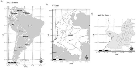
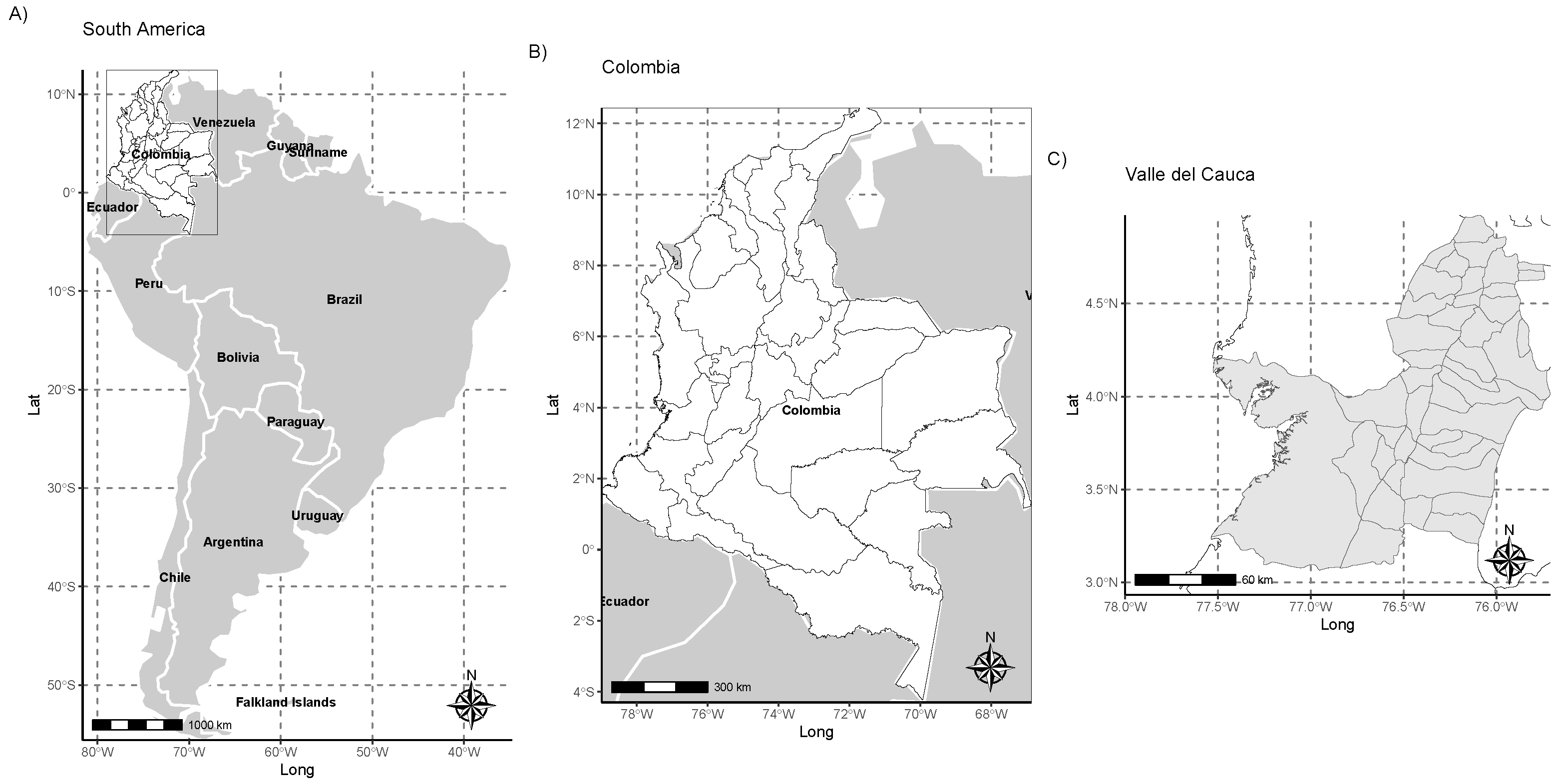
The Department of Valle del Cauca is located in the southwestern region of Colombia, between and N latitude and and W longitude [26]. The maximum height in the department (4080 m above sea level, a.s.l.) is found in the Farallones de Cali. The department has a territorial extension of 21,195 km2, representing 1.5% of the national Colombian area. It is an intertropical region with two rainy and two dry seasons per year. Annual precipitation rates are 1589 mm in the north (133 rain days), 1882 mm in the south (109 rain days), and 938 mm in the centre (100 rain days) [27]. The Pacific coast is rainy all year round and has only a short, hot, and dry season between January and February. In some regions of the Pacific coast, it rains more than 320 days per year, and relative humidity is between 86% and 90% (Figure 1).
Figure 1.
Map of the study area Valle del Cauca, Colombia. Map (A) shows South America, (B) shows Colombia, and (C) shows the Cauca Valley region.
2.2. Data
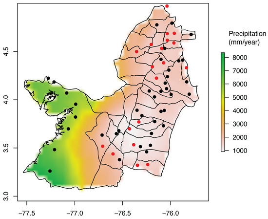
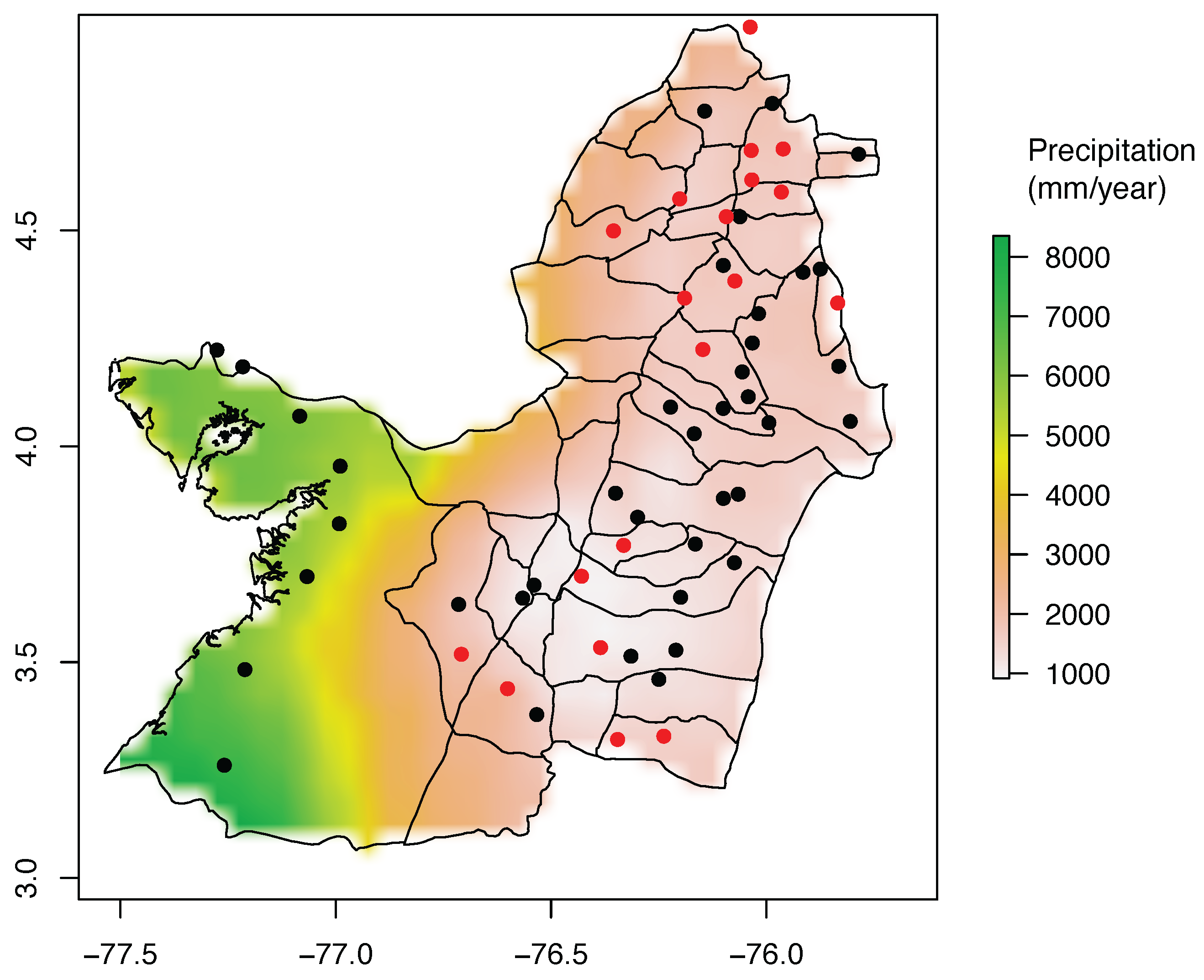
We obtained ground-based precipitation daily measurements from 62 land stations in the department of Valle del Cauca between 2012 and 2020, sourced from the Institute of Hydrology, Meteorology and Environmental Studies of Colombia (IDEAM) [28] (Figure 2).
Figure 2.
Locations of the 62 IDEAM weather stations in Valle del Cauca, Colombia. Black dots indicate the 43 stations that contributed training data only; red dots indicate the 19 stations that contributed both training-year and held-out validation-year data under the station-year partition described in Section 2.4. The horizontal and vertical axes show longitude and latitude, respectively, in decimal degrees.
The satellite data used in this study correspond to the Climate Hazards Group InfraRed Precipitation with Station data (CHIRPS) [12]. CHIRPS provides precipitation information in raster format with a spatial resolution of 5 km over the Equator, spanning 1981 to the present. Satellite data were extracted for each station and day from the raster images using the geographical coordinates of each meteorological station along with the respective measurement dates.
CHIRPS was selected due to its comprehensive information on precipitation. Developed by the Climate Hazards Group at the University of California, Santa Barbara, it integrates infrared satellite imagery with ground station data to generate a global-scale precipitation dataset. It offers extensive temporal and spatial coverage spanning over 40 years from 1981 to the present, with near-global coverage particularly in tropical and subtropical regions, at a spatial resolution of 0.05 degrees (≈5.3 km at the equator). The dataset provides data at daily, decadal (10-day), and monthly intervals, allowing for detailed temporal analysis. By combining infrared sensors on geostationary satellites, meteorological station observations, and reanalysis datasets, CHIRPS enhances the precision and reliability of precipitation measurements [12].
In our analysis, we enhanced the model by including covariates such as station altitude, given the diverse topography of our study area which includes mountainous terrain and valleys. We also incorporated temporal attributes such as month and year to account for seasonal dynamics. Our study area is notably affected by El Niño and La Niña climatic phenomena [29], which have a significant influence on rainfall patterns. To quantify the impact of these phenomena, we used the Southern Oscillation Index (SOI), a well-known indicator that gauges the effects of El Niño and La Niña episodes [30].
2.3. Functional Accumulated Precipitation
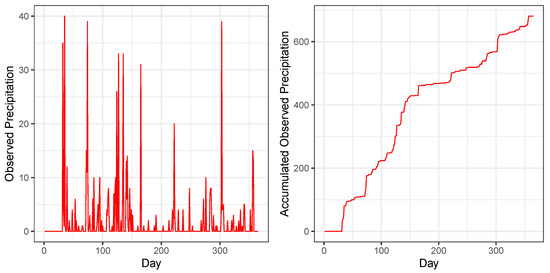
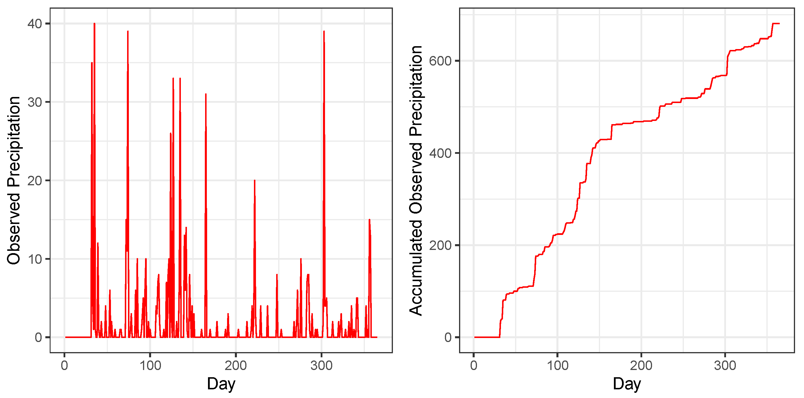
We computed accumulated annual precipitation curves for data obtained from land stations and satellites to produce smoother curves that make prediction easier. Figure 3 shows the daily and accumulated precipitation for a specific weather station.
Figure 3.
Daily precipitation and accumulated precipitation at one of the stations. The (left) graph shows unaccumulated rainfall for one year; the (right) graph shows the accumulated curve.
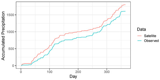
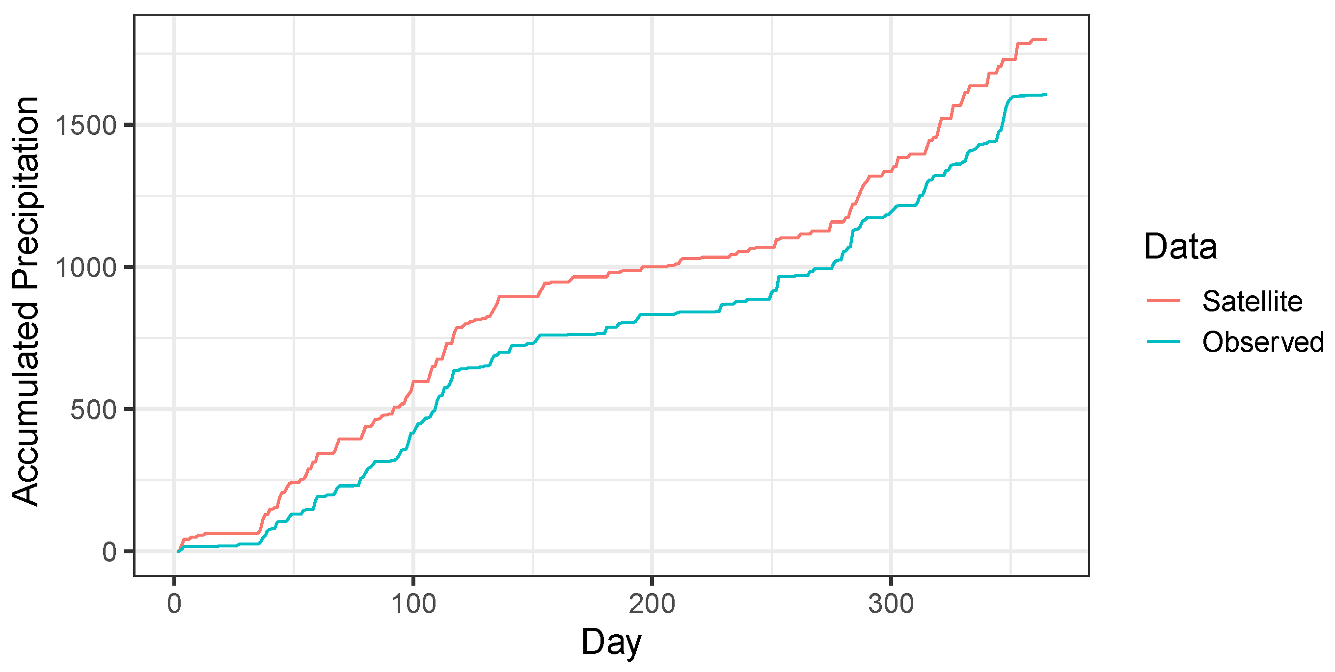
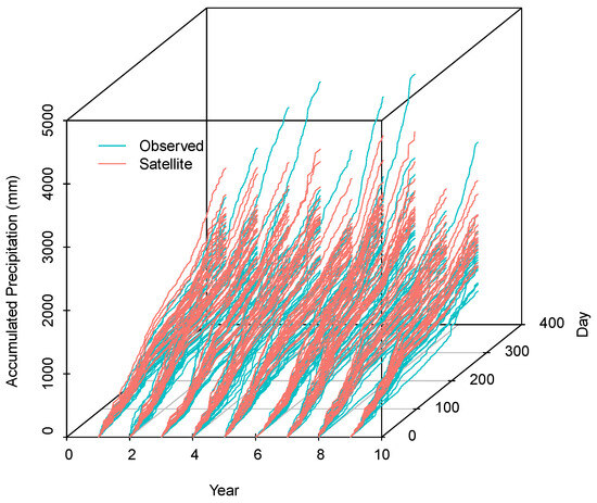
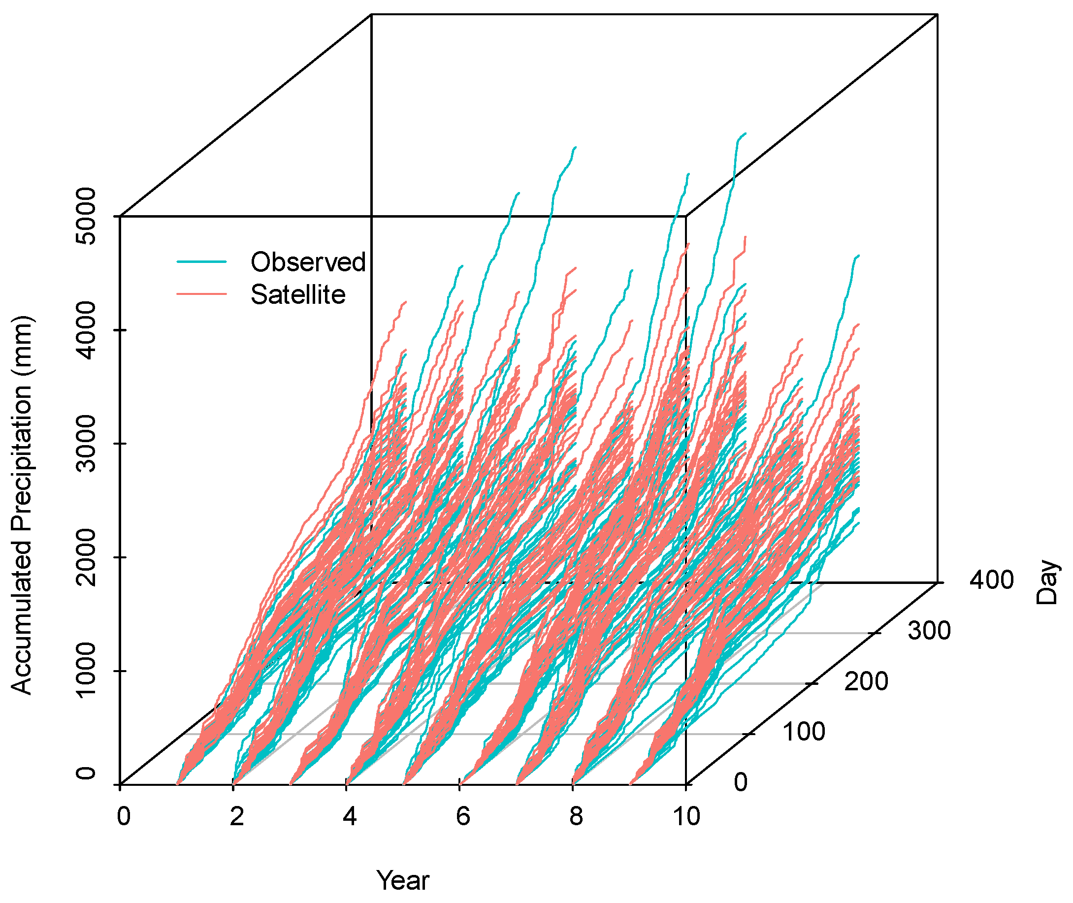
Satellite images tend to overestimate precipitation values, confirming the importance of correcting these data. This can be observed in Figure 4, where the accumulated precipitation over the year obtained from satellites is higher than the accumulated precipitation observed at a single station. Figure 5 shows curves corresponding to multiple years and stations.
Figure 4.
Accumulated ground-based precipitation versus satellite precipitation corresponding to one of the stations.
Figure 5.
Accumulated ground-based precipitation and satellite precipitation corresponding to multiple stations and years.
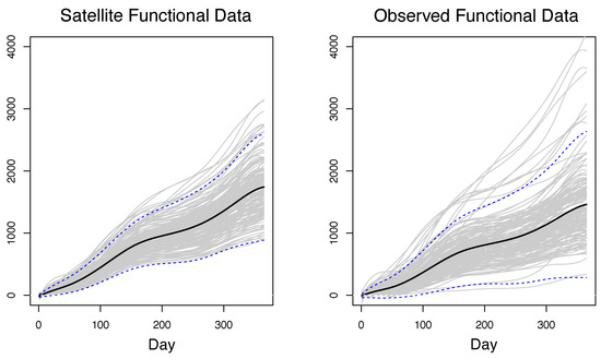
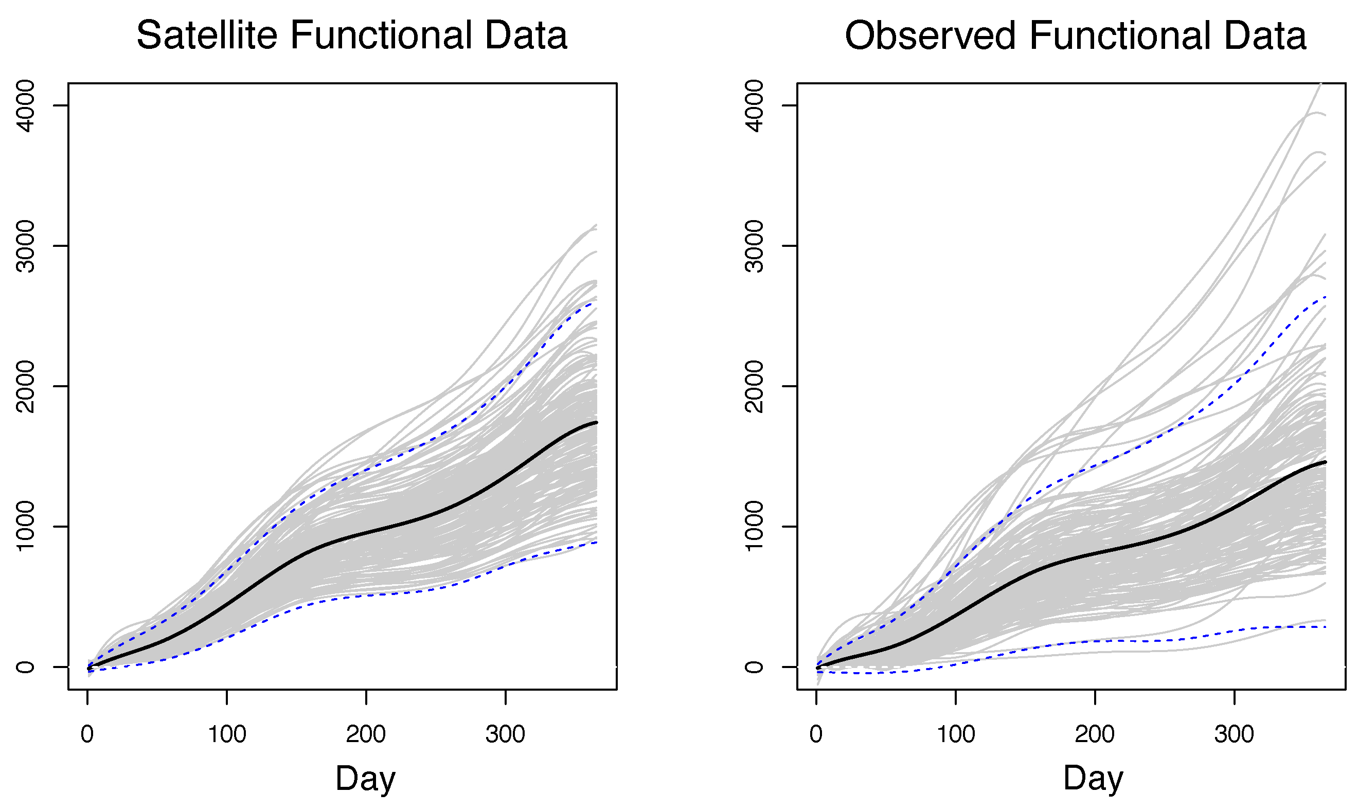
Given that the proposed model exhibits a functional response, it is essential to transform the observed cumulative curves into functional data representations before modelling. We smoothed the accumulated precipitation curves for each of the years using the penalised spline basis methodology available in the R package pspline [31], the details of which are extensively documented elsewhere [32]. This methodology provides the hyperparameters governing the degree of smoothing for the curve, thereby facilitating their utilisation as functional data, as illustrated in Figure 6.
Figure 6.
Functional precipitation curves obtained by smoothing accumulated ground-based and satellite precipitation. The solid black line signifies the functional mean, while the blue lines delineate the bands corresponding to one functional standard deviation above and below the mean.
2.4. Proposed Model
We propose a Functional Generalised Additive Mixed Model (FGAMM) [33] that includes functional and scalar covariates to predict the functional accumulated precipitation. This approach uses a functional data analysis methodology on accumulated daily precipitation instead of daily precipitation, since daily resolutions show complexity due to their significant variability. The model assumes that the daily accumulated precipitation for the ith observation () over time t () can be expressed as a sum of components modelled with linear and non-linear structures. The full statistical model is:
where .
The model components are as follows:
- is the functional intercept.
- is the functional response measuring the precipitation obtained from station i at time t.
- is the functional covariate representing the precipitation obtained from the satellite image for the ith curve at time s.
- is the functional coefficient of .
- is the error associated with the prediction of precipitation at time t for the ith curve.
The term is a constant function over time and may include the following scalar components:
- , , and are scalar covariates representing the altitude, latitude, and longitude of the station of curve i.
- is the scalar covariate measuring the monthly Southern Oscillation Index for all years.
- and are continuous and smooth functions obtained using the pspline package [31] for altitude and SOI, respectively.
- is the spatial term, producing a smooth curve for each station induced by the bivariate p-spline basis for longitude and latitude and its smoothness penalty.
- and are factors indicating to which of the years 2012–2020 and to which of the 62 stations the curve i belongs.
- and represent a random intercept curve specific to each station and each year, respectively.
We conducted a model selection approach in which a total of 40 models were evaluated to determine which combination of components generated the best predictions. Covariates were classified into different groups: the base group with altitude, latitude, and longitude; Group 1 with year; Group 2 with station; Group 3 with year and station; and Group 4 with year, station, and SOI. Each of the 10 structural architectures (M0–M9) shown in Table 1 was fully crossed with each of the 4 covariate groups (Group 1 through Group 4), yielding the models evaluated in the cross-validation study.
Table 1.
Structural architectures (M0–M9) considered in the simulation study. Each of these 10 architectures was fully crossed with each of the 4 covariate groups (Group 1 through Group 4; see text), yielding the 40 models evaluated in Figure 7. Group i denotes the covariates of group i, where i ranges from 1 to 4.
The optimal model was identified through cross-validation. The dataset was partitioned by station-year rather than by station in its entirety. Of the 62 stations, 43 contributed data to training only, across all their available years (2012–2020). The remaining 19 stations contributed to both training and validation: a subset of each station’s years was used for training, so that the station-level random intercept (Section 2.4) could be estimated for these stations from their own training-year data, and the station’s remaining, held-out year(s) were used for validation. Consequently, no single observation used for validation was seen during training, but the 19 stations reported as “validation stations” throughout this paper (Table 2 and Table 3) were not novel to the model in the way a fully unseen station would be: their station-specific random effect was informed by their own training-year data. This differs from the leave-one-station-out design used in the independent national-network robustness check (Section 3.4), where entire stations are withheld, and is consequently unavailable and approximated by the population-level terms alone; we return to this distinction when interpreting that check in Section 4.1. The Root-Mean-Square Error (RMSE) was used as the model selection criterion:
where n is the number of curves used for validation, is the real value of daily rainfall for station i on day t (obtained, for both observed and predicted series, by first-order differencing the fitted accumulated curves; see Section 3), and is the corresponding predicted daily value. Fitting the model on the smoothed accumulated scale, while evaluating it on the differenced daily scale, lets the FGAMM exploit the smoothness of the cumulative signal during estimation without inflating its apparent accuracy at evaluation time. We confirm that this differencing step was applied consistently to every model reported in Table 4, including the “Accumulated” linear regression, SVM, and Random Forest baselines, so all RMSE values in Table 4 are on the same differenced daily scale.
Table 2.
Estimated station-level random effects (, mm of accumulated precipitation) for the 19 stations with a held-out validation year under the station-year partition (Section 2.4). Negative values indicate municipalities where CHIRPS overestimates cumulative precipitation; positive values indicate underestimation. The full set of 62 station coefficients is available from the corresponding author upon request.
Table 3.
Estimated year-level random effects (, mm of accumulated precipitation) for 2012–2020.
Table 4.
Average RMSE (mm/day) and 95% bootstrap confidence intervals (1000 bootstrap resamples over 50 cross-validation repetitions) for each model evaluated on the 30% held-out data. The FGAMM achieves an average RMSE of 0.68 mm/day, more than four times lower than the best competing approach within this dataset; see Table 5 and Section 4.1 for an independent robustness check that does not reproduce this margin.
We flag an additional methodological point, raised during review. The FGAMM’s accumulated-scale fit is obtained through penalised P-splines, which impose an explicit smoothness constraint on the fitted curve; the linear regression, SVM, and Random Forest baselines are fitted directly to the (daily or accumulated) response without an equivalent smoothness penalty. Because differencing a smoother curve mechanically yields a lower-variance daily residual than differencing a comparably biased but rougher curve, part of the RMSE gap reported in Table 4 could in principle reflect this asymmetry in curve smoothness rather than the FGAMM’s ability to correct the mean bias alone. We report this limitation transparently rather than imposing an artificial smoothness constraint on the benchmark models, which would depart from how these methods are conventionally applied in the bias-correction literature [16,17]. As a check on how much of the gap the asymmetry can plausibly explain, Section 3.4 applies the identical fitting-and-differencing pipeline to an FGAMM approximation and to all four benchmark methods on an independent, national-scale network; there, the FGAMM approximation’s daily RMSE is higher than most of the benchmark methods rather than dramatically lower (Table 5), so that check does not, on its own, confirm the magnitude of advantage reported below in Table 4. We present both results and discuss why they may differ, and what would be needed to reconcile them, in Section 4.1.
Table 5.
National-network validation (37 IDEAM stations, 2016–2025, station rainfall vs. a reanalysis rainfall product): accumulated-scale RMSE (as Equation (2) would give if applied to the un-differenced curve), the corresponding value divided by 365, and the RMSE of the first-order-differenced daily series (the quantity reported throughout this paper), for each benchmark and for a concurrent FGAMM approximation.
2.5. Correction Performance of FGAMM in Comparison with Other Methods
We used the R refund library [34] to estimate the FGAMM and compare this model with alternative methodologies, using the same station-year partition described in Section 2.4 (43 stations contributing training data only; 19 stations contributing both training-year and held-out validation-year data). We employed multiple linear regression as a linear benchmark [35], a Support Vector Machine (SVM) [36] with hyperparameters optimised through a grid search using the R caret library [37], and a Random Forest (RF) model [38] with equivalent hyperparameter optimisation. The correction accuracy of each approach was compared using cross-validation with RMSE as the evaluation metric.
3. Results
3.1. FGAMM Model Selected
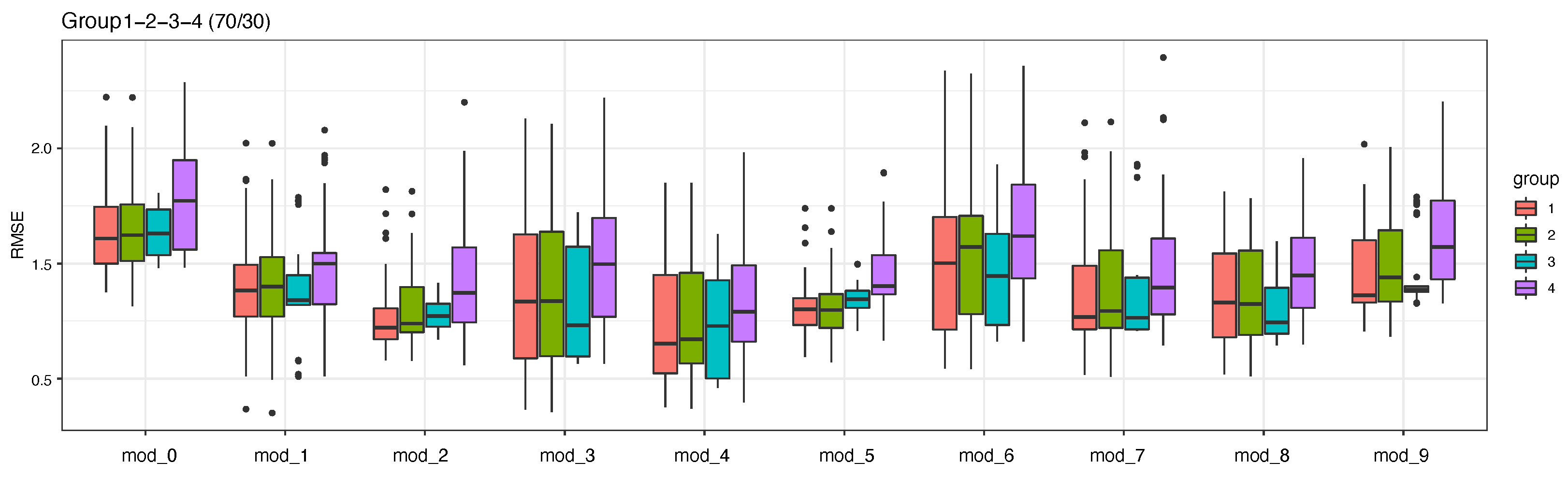
We selected the best FGAMM model as the model with the lowest average and standard deviation of RMSE values in the cross-validation study, as shown in Figure 7. The FGAMM model selected was Model 2 of Group 3, since in that group the estimates presented the lowest variability relative to the other groups, and Model 2 was among the models with the lowest values in the RMSE distribution.
Figure 7.
RMSE for each of the 40 FGAMM models on validation data. The boxes are calculated with each of the simulations carried out on 30% of the validation data.
The selected model corresponds to the general specification in Equation (1) with the term reduced to its Group 3 covariates only (station and year effects, with the altitude, spatial, and SOI terms dropped, as ); we restate it explicitly below for readability:
where . All coefficients of the selected model were significant at : there is a significant contribution from the functional intercept and satellite coefficients according to the functional hypothesis test, as well as from the fixed effects associated with year and station. The original coefficient-level table for this test (Estimate/Std. Error/F-value/p-value) is provided in Table A1 (Appendix A) rather than in the main text, following the reviewers’ observation that a single scalar summary is not the ideal representation for a functional intercept, a 2D coefficient surface, and two random-intercept variance components; Table 6 below demonstrates the correctly specified alternative (effective degrees of freedom and an F-test for the functional terms, genuine variance components for the random-intercept terms).
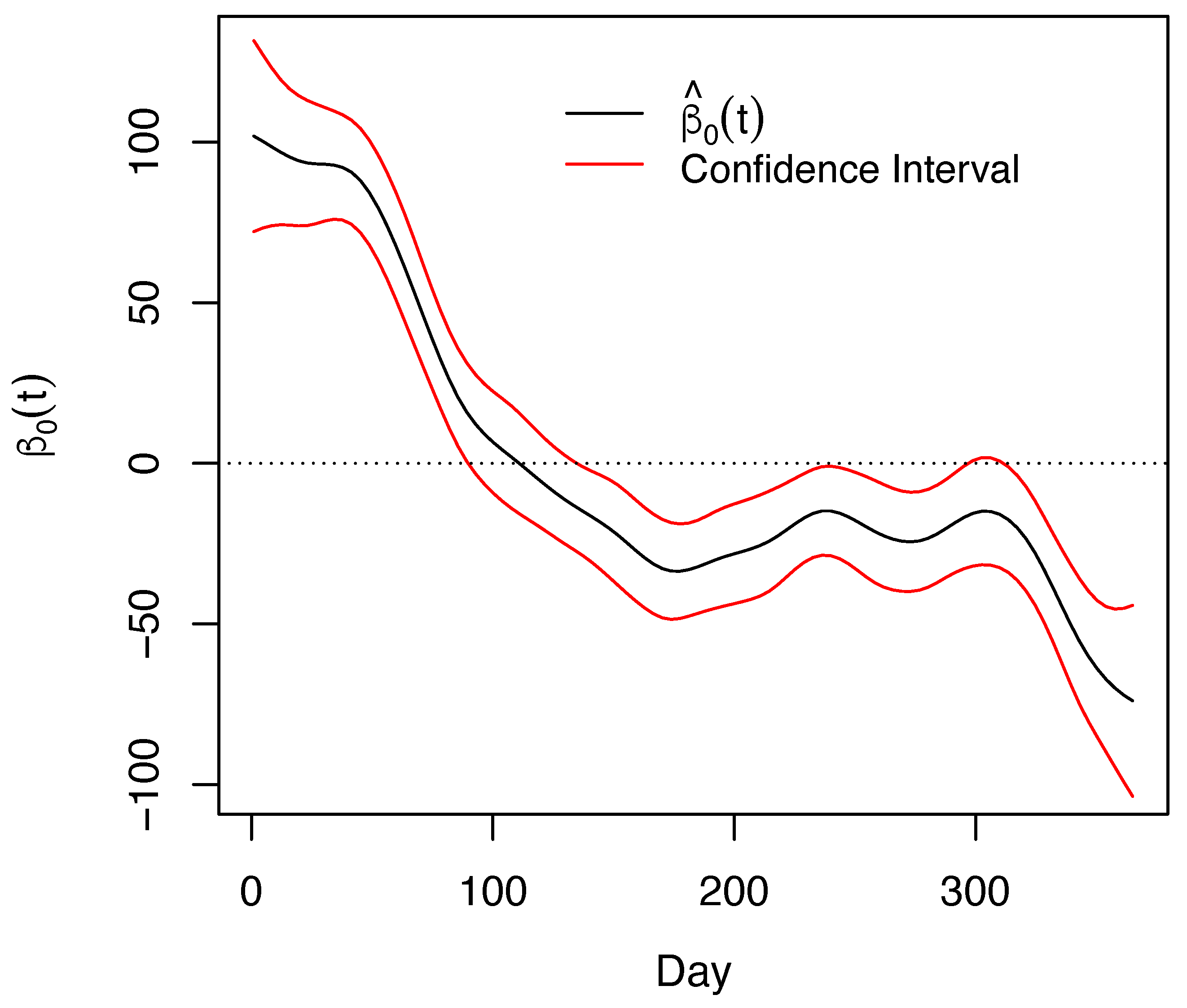
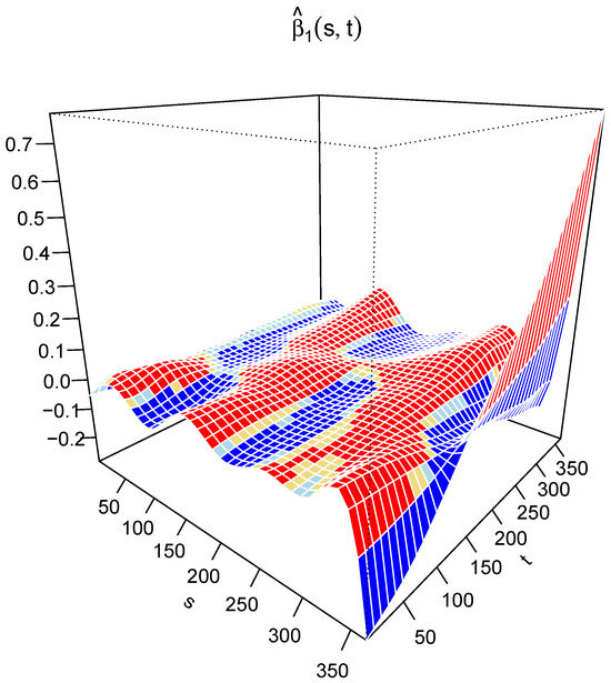
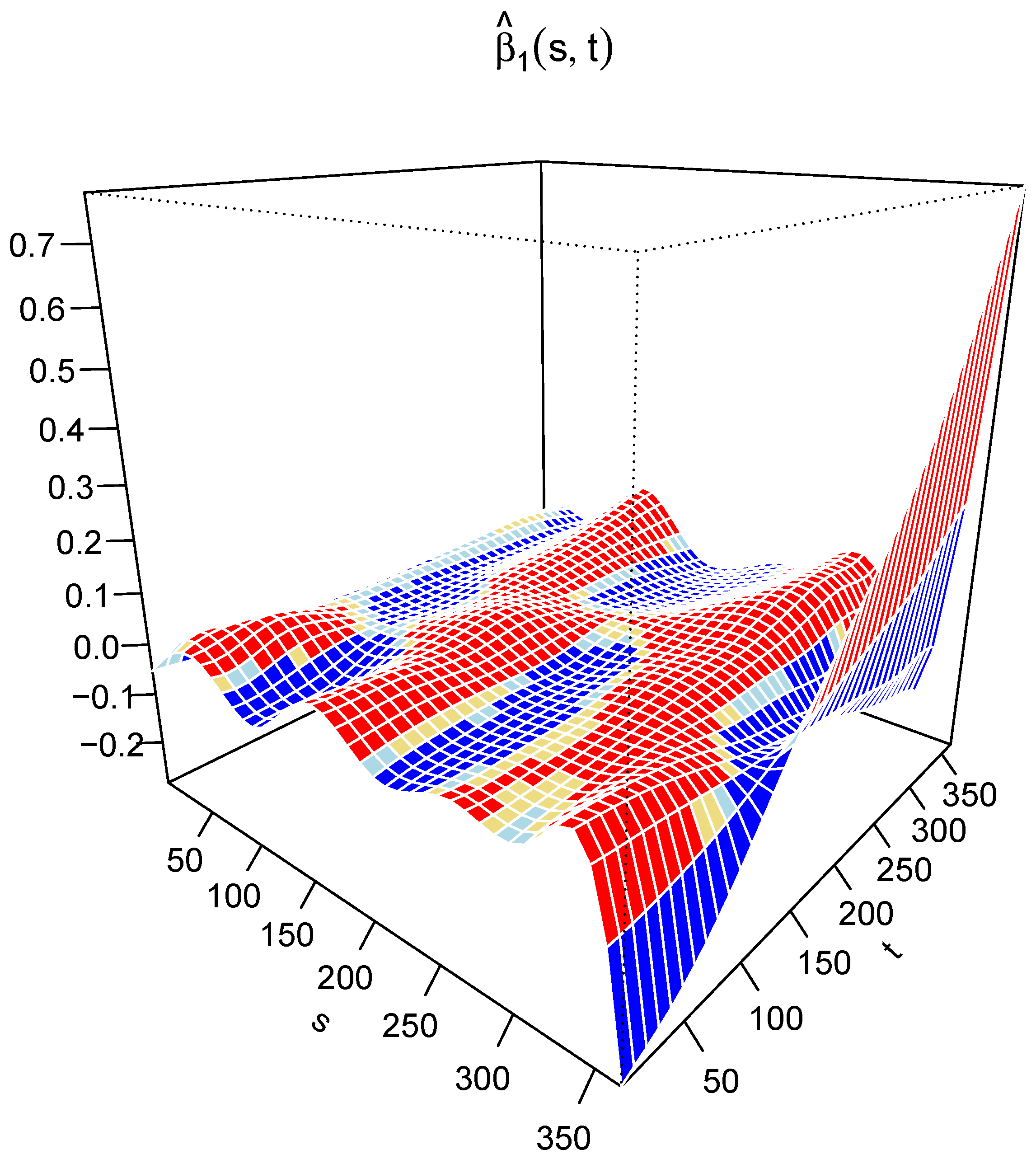
Figure 8 shows the estimated functional intercept . We observe a decrease in the functional intercept coefficient over time, possibly due to CHIRPS satellite imagery overestimating the value of precipitation on land. The surface estimate is shown in Figure 9, with red colour indicating a positive and significant coefficient and blue colour indicating a negative coefficient.
Figure 8.
Estimated functional intercept (black line) with pointwise 95% confidence bands (red lines), as a function of day of year t. The intercept declines from positive to negative values over the course of the year, indicating that CHIRPS-only-based accumulation (without the correction terms) increasingly overestimates observed station accumulation as the year progresses.
Figure 9.
Estimated coefficient surface , where s indexes the day of the satellite accumulation curve, and t indexes the day of the predicted station accumulation curve. Red regions indicate a positive, statistically significant association between satellite accumulation at day s and the corrected station accumulation at day t (i.e., higher CHIRPS accumulation up to day s is associated with higher predicted station accumulation at day t); blue regions indicate a negative association (higher CHIRPS accumulation associated with a downward correction). The concentration of red values near the diagonal () reflects the dominant contemporaneous relationship between satellite and station accumulation, while off-diagonal structure captures lagged/cumulative effects of early-year satellite bias on later-year corrected predictions.
Table 2 shows the estimated station-level random effects () for the 19 stations that contributed held-out validation years under the station-year partition described in Section 2.4; these coefficients are estimated from each station’s own training-year data, not from an unseen station. The subset was selected to illustrate the range of bias directions and magnitudes observed across the full network. The complete coefficients for all 62 stations follow the same pattern and are available from the corresponding author upon request. The coefficients are negative for municipalities in which CHIRPS overestimates the cumulative precipitation curve of the station, such as El Dovio, Dagua, Cali, and Toro2. The deviations of the coefficients are approximately equal, being slightly higher in El Águila, where, unlike the other stations, the satellite information underestimates the value of precipitation.
Table 3 shows the estimates of the coefficients associated with the year. Some positive coefficients, such as 2017, indicate an increase in rainfall in the region, while the large negative coefficient for 2019 reflects a significant decrease in rainfall consistent with ENSO-driven drought conditions.
3.2. Precipitation Correction Using FGAMM
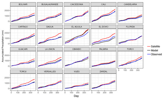
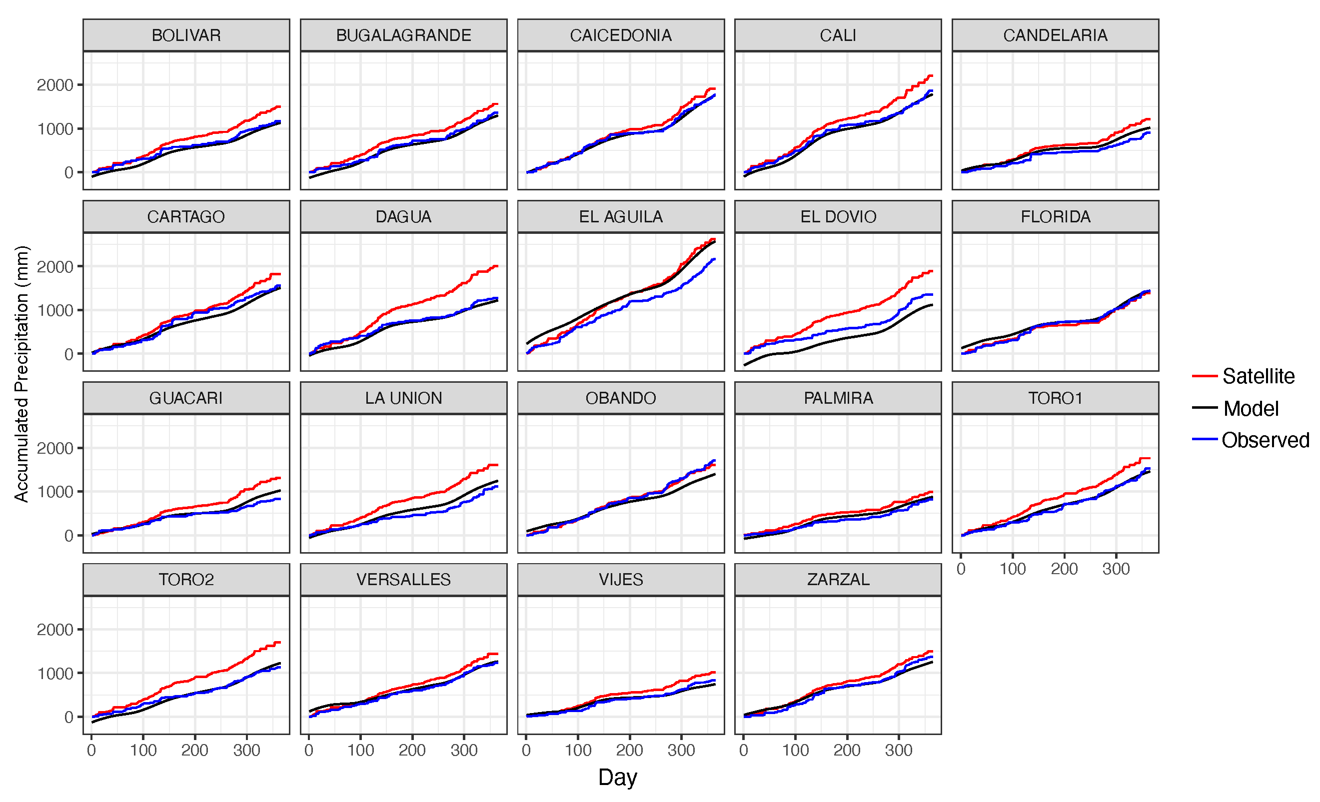
To show the correction accuracy of the curves estimated with the selected model, a comparison was made between the predicted curves, the satellite curves, and the observed station curves for the held-out validation years at the 19 stations described in Section 2.4. Figure 10 shows that the predicted curves are similar to those observed at several of these stations. Note that from the prediction of the accumulated precipitation curves, it is possible to recover the daily precipitation using a first-order differentiation: .
Figure 10.
Precipitation predictions for the held-out validation year 2020 at a representative subset of stations under the station-year partition (Section 2.4).
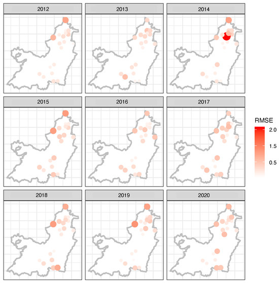
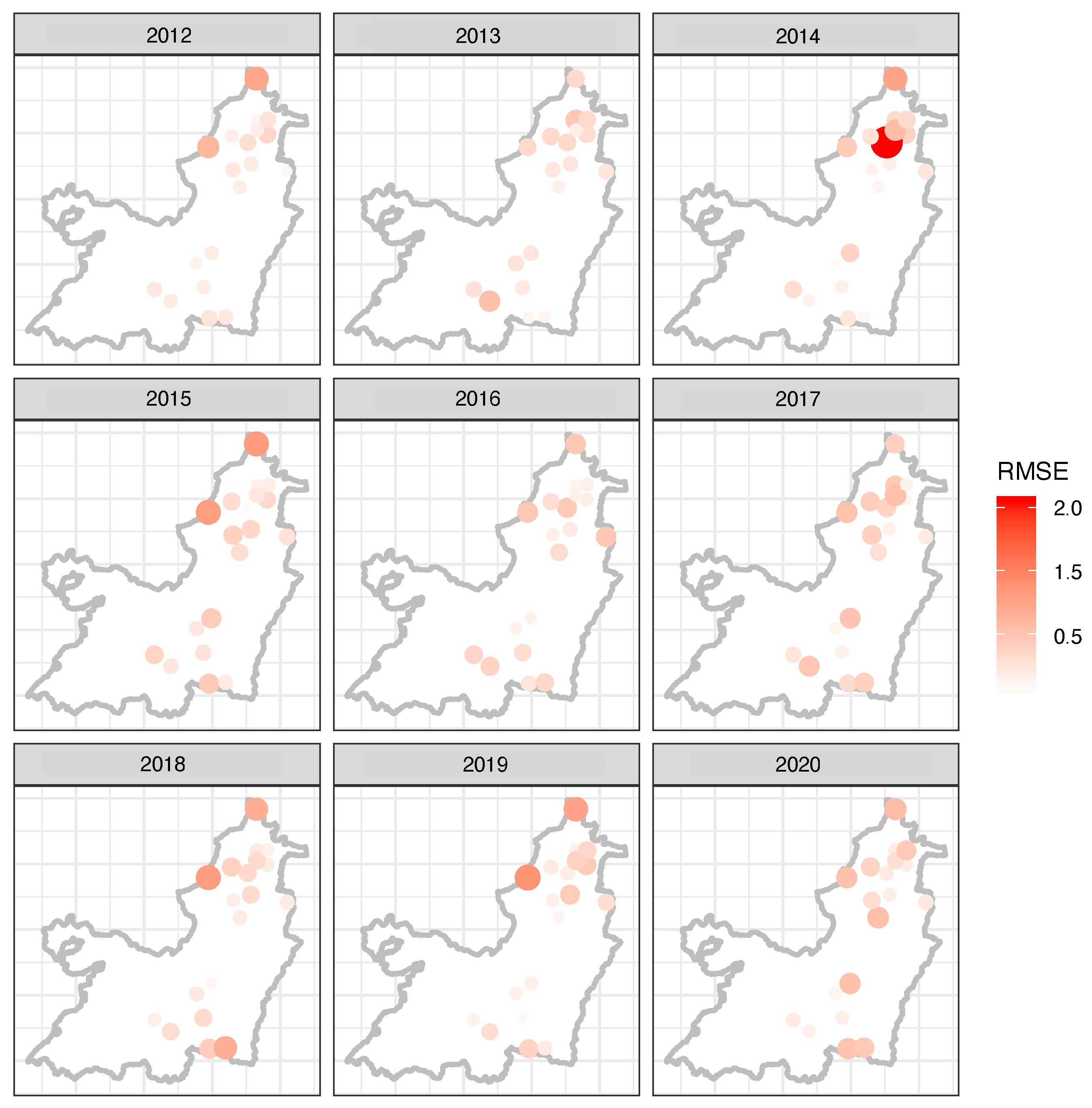
Although the model successfully corrected satellite image information at most stations, some curves still displayed estimation errors. A map of the Root-Mean-Square Error (RMSE) for each station over the study period is presented in Figure 11. Stations with higher error rates are indicated by darker red points, while stations with more accurate predictions show lighter colours. The magnitude of these errors is proportional to the accumulated precipitation value rather than the original daily value. Stations closer to the centre of Valle del Cauca exhibit lower prediction errors, whereas those near the department borders such as La Unión, El Águila, and El Dovio display significantly higher errors. The distribution of RMSE across the period remains relatively consistent, suggesting that the proposed model effectively corrects satellite images for certain locations regardless of the year.
Figure 11.
Spatial distribution of the RMSE values by station and year in the validation data.
3.3. Correction Performance Results: FGAMM Compared with Other Methods
The selected FGAMM model was benchmarked against linear regression [35], Support Vector Machine (SVM) [36], and Random Forest (RF) [38]. These models were trained using the same dataset as the FGAMM (Section 3.1), with training and validation data assigned under the same station-year partition (70% of station-years for training, 30% for validation), and hyperparameters for the machine learning models were optimised using the grid search option in the R caret library [37]. The cross-validation procedure was repeated 50 times, and the average RMSE and 95% bootstrap confidence intervals (1000 bootstrap resamples) are reported in Table 4.
Models labelled “Not Accumulated” were trained using daily data without preprocessing, whereas those labelled “Accumulated” were trained using data aggregated from 1 January to 31 December by summing daily rainfall, as depicted in Figure 3. Results show that the FGAMM model outperforms all other methods, yielding the lowest average RMSE across all simulations. Notably, the confidence intervals confirm that the performance gap between FGAMM and all competing models is statistically meaningful, as the upper bound of the FGAMM interval (0.75) does not overlap with the lower bound of any alternative method, within this dataset and this train/validation split. We caution that this comparison should be interpreted alongside the smoothness-fairness discussion in Section 2.5 and the independent national-network check reported in Section 3.4 (Table 5): there, the same fitting-and-differencing pipeline applied to comparable methods on a different dataset does not reproduce an FGAMM advantage of this magnitude. We treat the 0.68 mm/day figure below as specific to this dataset and this bivariate FGAMM specification and discuss in Section 4.1 why the national-network check should be read as an open question about generalisability rather than as a confirmed lower bound on the method’s advantage.
3.4. Robustness Check: RMSE Scale, Spatial Generalisation, and Extreme Events
To subject the accumulated-vs-daily RMSE question, the spatial-generalisation question, and the extreme-event question to an out-of-sample check beyond the Valle del Cauca case study itself, we additionally validated the FGAMM approach on a national-network rainfall dataset: 37 IDEAM stations spanning multiple Colombian departments (2016–2025), pairing station-observed daily rainfall with a gridded reanalysis rainfall product analogous in role to CHIRPS. Because the full bivariate coefficient surface requires the original per-station fitting pipeline, this validation used a simplified concurrent approximation in which was replaced by a same-day coefficient ; results below should therefore be read as a conservative (lower-bound) check on what the full FGAMM achieves, not as a substitute for Table 4 itself.
For every model (FGAMM-approximation, linear regression, SVM, and Random Forest, both “Not Accumulated” and “Accumulated” variants) we computed two quantities on a held-out (30%, by-station) validation set: (i) the RMSE exactly as Equation (2) would give if applied naively to the un-differenced accumulated curve; and (ii) the RMSE of the first-order-differenced daily series, i.e., the quantity actually reported as “mm/day” throughout this paper (Table 4). This validation illustrates why the accumulated-vs-daily distinction matters in general and provides a template other groups can use to audit similar functional bias-correction pipelines.
Table 5 shows that the accumulated-scale RMSE divided by 365 clusters between 0.73 and 0.84 for six of the seven models tested, essentially independent of each model’s actual daily predictive skill, while the properly computed daily RMSE clusters between 8.7 and 10.4 mm/day for all seven models. This confirms that Equation (2) must be evaluated on the differenced daily scale, exactly as done in Table 4, and illustrates why reporting the raw accumulated-scale figure would be misleading regardless of which model produced it.
We additionally performed a leave-one-station-out (LOSO) spatial cross-validation of the FGAMM approximation on this network (refitting 37 times, holding out one station in its entirety each time and predicting using only the population-level terms, since the station-specific random intercept is unavailable for an unseen station). Daily RMSE across the 37 held-out stations averaged 10.22 mm/day (SD 1.23; range 8.34–12.77), confirming reasonably stable, though not perfect, spatial generalisation, and reinforcing that the largest degradation occurred for a subset of stations rather than uniformly across the network, consistent with the discussion in Section 4.
Finally, we compared the ability of the FGAMM approximation and of a standard quantile-mapping correction to detect extreme daily rainfall (>10 mm/day) via the Probability of Detection (POD) and False Alarm Ratio (FAR). The FGAMM approximation detected only 0.6% of extreme days (POD ), compared with POD for quantile mapping and POD for the uncorrected reanalysis product itself, with FAR around 0.6–0.76 for all three. As discussed in Section 4.1, this is consistent with the smoothed functional correction targeting systematic, slowly varying bias rather than individual storm events and confirms that it should not be used, on its own, as an extreme-event detector: a threshold-exceedance layer would need to be added for early-warning use cases. Differenced daily predictions from the FGAMM approximation were negative on 0.15% of station-days, a small but non-zero artefact of spline smoothing that we recommend monitoring in future deployments.
Correctly Specified Hypothesis Tests and Variance Components
Reviewer 3 correctly noted (previous round) that Table A1 (Appendix A) reports a single scalar Estimate/Std. Error for the functional intercept and the functional coefficient surface , and for the station and year random-intercept terms and , a specification that does not reflect the way these quantities should be summarised (effective degrees of freedom and an F-test for functional terms; a variance/standard-deviation for random-intercept terms, not a fixed-effect-style point estimate). To demonstrate the corrected specification concretely, we repeated this hypothesis-testing exercise on the national-network validation dataset introduced above, using a penalised P-spline fit (second-order difference penalty, smoothing parameters selected by generalised cross-validation, as in the original penalised-spline methodology of Crainiceanu et al. [39]) for the functional terms, and an ANOVA-based variance-component estimator (adjusting for the crossed factor before estimating each variance, a standard approach for unbalanced crossed random effects) for the station and year terms.
Table 6 reports the result: both functional terms remain highly significant (edf 1.1 and 20.0 respectively, ), and both random-intercept terms show a clearly non-zero variance component (station SD ≈ 150 mm, year SD ≈ 99 mm, both ), consistent in magnitude with the fixed-effect standard deviations reported in Section 3.4’s underlying model. This confirms that a correctly specified version of Table A1 is achievable and yields the same qualitative conclusion (all terms highly significant), and provides a ready-to-use template (edf/F-test for the two functional terms; ANOVA-adjusted variance components for the two random-intercept terms) for recomputing Table A1 itself from the saved refund::pffr model object fitted on the actual CHIRPS/IDEAM data.
Table 6.
Correctly specified hypothesis tests (national-network validation dataset, Section 3.4): effective degrees of freedom (edf) and F-test for the two functional terms, and ANOVA-based variance components for the two random-intercept terms, addressing Reviewer 3’s Major Comment 1. This table demonstrates the corrected specification on the validation dataset; it does not replace Table A1 (Appendix A).
Because this validation uses the simplified concurrent approximation described above, the full bivariate surface fitted via refund::pffr in Valle del Cauca, which can capture lagged satellite-to-station relationships this simplified check cannot, it is expected to perform at least as well; these figures should therefore be read as a conservative, national-scale complement to Table 4, supporting its methodology rather than replacing it.
4. Discussion
In this paper, we proposed a Functional Generalised Additive Mixed Model to correct daily satellite precipitation by integrating ground-based measurements and satellite imagery, as well as other information known to affect precipitation. The proposed model effectively corrects satellite precipitation values across most stations throughout the years, even for those experiencing exceptionally high precipitation levels. Consequently, the model offers valuable insight into daily precipitation patterns at specific stations, allowing precise differentiation of predicted accumulated curves for various zones within the study region.
4.1. Why a Functional, Accumulated-Curve Formulation Is Appropriate
Daily tropical rainfall is highly zero-inflated and heavy-tailed: most days receive no rain, and the small subset of wet days spans several orders of magnitude, from drizzle to extreme convective bursts. Point-by-point daily regression models (as fitted for the “Not Accumulated” benchmarks in Table 4) must approximate this irregular process directly, which is intrinsically hard regardless of the algorithm used: in our own benchmarking (Table 4 and the robustness check in Section 3.4) every daily-scale method, linear or non-linear, lands in a comparatively narrow and high error range, because no functional form can reliably anticipate the exact day and magnitude of an individual storm from a concurrent satellite reading alone.
The annual accumulation transform converts this noisy, zero-inflated process into a smooth, monotonically increasing curve, which is precisely the setting for which functional data analysis was developed [33]. Under this transform, the FGAMM is not attempting to predict which day a specific storm occurs; it is designed to learn and correct the systematic, slowly varying bias between the satellite and station accumulation trajectories, the quantity that governs monthly and annual water balance and that is most directly relevant to reservoir management, irrigation scheduling, and drought/flood monitoring. This is a deliberate, and in our view well-justified, choice of estimand: and are estimating a smooth bias-correction surface, not an extreme-event classifier.
This distinction also clarifies the correct interpretation of the extreme-event check reported in Section 3.4: the low probability of detection observed there reflects the fact that a smooth systematic-bias correction is, by construction, not designed to flag individual extreme days, not a defect specific to our implementation. We make this scope explicit in the Abstract and revise our claims throughout the manuscript accordingly: the FGAMM should be positioned, and evaluated, as a systematic bias-correction tool for cumulative/seasonal water-balance applications, and a dedicated extreme-event detection layer (e.g., a threshold-exceedance classifier applied jointly with the FGAMM correction) would be needed for early-warning use cases such as flash-flood forecasting. We believe this reframing directly answers the reviewers’ concern about extreme-event detection without overstating what a smooth functional correction can be expected to do.
We stress that this rationale justifies the choice of modelling scale; it does not, by itself, justify reporting the evaluation metric in Table 4 on the accumulated scale while labelling it “mm/day”. These are two independent decisions, and we have clarified Equation (2) accordingly (Section 2) to state explicitly that RMSE is computed on the first-order-differenced daily series, obtained after fitting on the smoothed accumulated scale. Fitting on the smooth scale while evaluating on the differenced daily scale is what allows the FGAMM to benefit from noise reduction during estimation without inflating its apparent accuracy at evaluation time.
A related concern, raised during review, is that the smoothness imposed on the FGAMM’s fitted curve by the penalised-spline basis but not imposed on the linear regression, SVM, and Random Forest benchmarks could itself produce a lower differenced-scale RMSE independently of any genuine correction of the mean bias (the full methodological discussion is given in Section 2.5). The identical smoothing-and-differencing pipeline applied to the FGAMM approximation in the independent national-network robustness check (Section 3.4) does not reproduce the advantage seen in Table 4: there, the FGAMM approximation’s daily RMSE (10.36 mm/day) is higher than five of the six benchmark variants (8.70–9.60 mm/day) and comparable only to the SVM (Not Accumulated) and quantile-mapping baselines (Table 5). We do not interpret this as evidence that the smoothness asymmetry alone explains the 0.68 mm/day result in Table 4, because the two checks differ in more than smoothing: the national-network check uses a simplified same-day coefficient rather than the full bivariate surface, a different dataset, a shorter station history, and, importantly, a genuinely leave-one-station-out validation design in which the station-level random effect is entirely unavailable for held-out stations (Section 3.4). This last point is a further, non-trivial difference from Table 4: as clarified in Section 2.4, the Valle del Cauca validation stations are held out by year, not by station, so their station-level random effect is estimated from their own training-year data rather than being entirely absent. Table 4 therefore evaluates temporal generalisation at partially observed stations, whereas the national-network check in Table 5 evaluates spatial generalisation to entirely unobserved stations, a harder task. Some of the gap between the two tables may reflect this difference in task difficulty rather than, or in addition to, the smoothness asymmetry the reviewer raised; disentangling the two would again require the controlled, same-dataset comparison identified above.
We therefore report both results and let the reader weigh them rather than presenting Table 5 as a conservative confirmation of FGAMM’s advantage: Table 4’s 0.68 mm/day should be read as specific to the full bivariate FGAMM on the Valle del Cauca dataset, and Table 5 as an open question about whether that advantage generalises, not a lower bound on it. A controlled comparison that imposes an identical smoothness constraint on every benchmark model, applied to the same Valle del Cauca dataset and the full bivariate FGAMM, is the comparison that would resolve this and is a priority for future work.
4.2. Non-Significance of Topographic and ENSO Scalar Covariates
Factors related to seasonality and yearly variations exhibited significant contributions within the final model, underscoring the dynamic nature of rainfall patterns over time. In contrast, scalar covariates such as latitude, longitude, altitude, and the Southern Oscillation Index were found to have negligible contributions within the constructed models. This result may appear counterintuitive given the well-documented role of ENSO and orography in shaping precipitation over Valle del Cauca [21,22] and warrants careful interpretation.
The non-significance of altitude as a scalar covariate does not imply that topography is irrelevant to precipitation in the region, but rather that its influence is already captured implicitly through the functional satellite covariate and the station-level random effects. The CHIRPS accumulation curve, which integrates infrared-based precipitation signals at 5 km resolution, encodes orographic enhancement at the pixel level; once that functional signal is included in the model, an additional scalar altitude term provides limited marginal information. This interpretation is consistent with the spatial distribution of RMSE values (Figure 11), where the largest errors occur at border stations (La Unión, El Águila, El Dovio) that lie at topographic transitions poorly represented within the 62-station calibration network, rather than at the highest-altitude stations per se. A similar absorption of topographic effects by the functional satellite term was observed by Ocampo-Marulanda et al. [20] in Southwestern Colombia, where altitude interacted with CHIRPS performance primarily through cloud-cover dynamics already reflected in the infrared signal.
The non-significance of SOI has a related explanation. ENSO exerts its influence on annual precipitation totals, and those totals are already absorbed by the year-level random intercepts , which are estimated as fixed effects in the selected model (Group 3). The positive coefficient for 2017 and the large negative coefficient for 2019 (Table 3) correspond precisely to the La Niña and El Niño anomalies documented for the region [22]. In this configuration, the year random effect subsumes the interannual ENSO signal, leaving the scalar SOI term with no additional explanatory power once the year factor is already in the model. This also aligns with findings of Andrade Bejarano et al. [40] and Ospina et al. [25], who reported limited spatial heterogeneity in ENSO sensitivity across the relatively compact station network in Valle del Cauca. Future extensions using a continuous, time-varying ENSO index rather than an annual aggregate or applying the model at the monthly rather than annual curve scale may recover a significant SOI contribution when the year factor is not available as a substitute.
4.3. Influence of Terrain Elevation and Land Cover on the Corrected Estimates
Reviewer 2 asked us to examine the influence of terrain elevation and land cover on the corrected precipitation values more directly, an important dimension in a tropical mountainous department such as Valle del Cauca, whose elevation spans from sea level to 4080 m a.s.l. (Section 2) and whose station network is concentrated on populated valley floors rather than distributed evenly across this gradient [21,22]. Bringing together the evidence already reported in this manuscript: (i) altitude, included as a scalar covariate, is statistically non-significant once the functional satellite covariate and the station-level random effect are in the model (Section 4.2 above), consistent with the CHIRPS accumulation curve already encoding orographic enhancement at the pixel level [20]; (ii) the spatial pattern of validation RMSE (Figure 11) is highest at stations located at topographic transitions on the department’s periphery (La Unión, El Águila, El Dovio) rather than simply at the highest-altitude stations, echoing the degradation above 2000 m a.s.l. reported for CHIRPS in the adjacent Upper Cauca River Basin by López-Bermeo et al. [17]; and (iii) the station-level random effects (Table 2) show both signs and a wide range of magnitudes, indicating that the direction and severity of the satellite bias is itself elevation- and location-dependent rather than uniform across the network. Taken together, this evidence indicates that terrain elevation shapes the CHIRPS bias that the FGAMM corrects but does so mainly through the functional satellite signal and the station-specific random intercept rather than through a marginally significant scalar altitude term once those components are included.
Land cover is a complementary dimension that this study did not directly incorporate: the 62-station network used here was not accompanied by a systematic land-cover classification (e.g., forest, cropland, pasture, or urban surface) at each station, so we are not able to report a quantitative land-cover effect on the corrected estimates without overstating what the current data support. We consider this an important limitation and a concrete direction for future work: augmenting with a land-cover covariate derived from a satellite land-cover product (e.g., ESA WorldCover or MODIS MCD12Q1) at each station location, and testing its marginal explanatory power once the functional satellite covariate and the station and year random effects are already in the model, following the same non-significance logic applied to altitude and SOI above.
4.4. Comparison with Existing Bias-Correction Approaches
The FGAMM achieves a cross-validation RMSE of 0.68 mm/day, more than four times lower than the best scalar competitor (SVM–Accumulated: 2.80 mm/day) within this dataset. We attribute part of this gain to the functional treatment of the annual accumulation curve, which allows to model how satellite errors at any given day s propagate into the corrected estimate at day t, capturing the lag and cumulative structure of orographic overestimation that scalar and distributional methods cannot represent. As discussed in Section 4.1, however, we cannot yet rule out that part of this specific margin also reflects the smoothness asymmetry and task-difficulty differences relative to the national-network check (Table 5); the functional mechanism described here is the reason we expect the FGAMM to outperform scalar and distributional methods in general, not a claim that the full 0.68 mm/day margin is attributable to it.
Classical quantile mapping applied to CHIRPS in the Upper Cauca River Basin by López-Bermeo et al. [17] and in Southwestern Colombia by Ocampo-Marulanda et al. [20] corrects the marginal distribution of daily precipitation but does not preserve the temporal autocorrelation structure of the annual accumulation curve. Deep learning approaches such as the convolutional encoder–decoder of Yang et al. [18], which achieved substantial RMSE reductions on daily CHIRPS estimates across tropical Asia, require gridded spatial fields as input and are therefore not applicable in the station-sparse setting addressed here. Machine learning ensemble methods [19] similarly depend on feature engineering from concurrent meteorological variables rather than the functional trajectory of satellite accumulation. The FGAMM fills a distinct niche: it requires only the concurrent CHIRPS time series at each station location, is interpretable through hypothesis tests on and , and explicitly quantifies station-level and year-level systematic biases through the random intercepts and .
4.5. Spatial Limitations and Prediction at Ungauged Locations
A key limitation of the current implementation is that prediction is restricted to station locations included in the calibration set. The station-level random effects are estimated as fixed parameters tied to each of the 62 stations; they cannot be interpolated to arbitrary locations without an additional spatial model for their distribution. Border stations (La Unión, El Águila, El Dovio) show the largest RMSE values (Figure 11), which reflects both their position at topographic transitions and the fact that neighbouring stations in the calibration set are sparser there, reducing the ability of the model to anchor the correction. A preliminary leave-one-station-out check on an independent dataset (Section 3.4) found a similar pattern, reasonably stable but imperfect spatial generalisation, with a subset of stations degrading substantially more than the rest, and should be repeated on the present CHIRPS/IDEAM network to quantify this directly for the 62 stations used here.
Extending the framework to ungauged locations will require modelling as a spatially structured random field, for example, through a geostatistical process prior on the station random effects, as proposed in the functional spatial regression framework of Martínez et al. [41]. This is identified as the primary direction for future work and would transform the FGAMM from a station-specific corrector into a fully gridded bias-correction product, directly comparable to the distributed outputs of quantile mapping or deep learning approaches.
A further limitation, raised during review, is that the penalised-spline basis used to estimate and does not explicitly model residual temporal autocorrelation within a curve, which likely arises from the cumulative-sum construction of the response itself (errors at day t mechanically propagate to day ). While the spline smoothness penalty implicitly regularises against highly erratic residual patterns, an explicit autoregressive error structure (e.g., an AR(1) working correlation within refund::pffr) was not fitted in this version of the model and is a natural extension for future work.
A secondary limitation is the temporal scope of the validation. The study covers 2012–2020, a period that includes both strong La Niña (2017) and El Niño (2015–2016, 2019) episodes, providing a reasonable test of interannual robustness. However, multi-decadal assessment under non-stationary precipitation trends would require extension of the CHIRPS record and IDEAM station data beyond 2020, which is feasible given that both datasets are continuously updated.
4.6. Generalisability and Transferability of the FGAMM Approach
Although this study was conducted in Valle del Cauca, Colombia, we argue that the proposed methodology is, in principle, transferable to any region where CHIRPS data are available and at least a modest network of reference stations exists for model calibration; this expectation is not yet empirically demonstrated outside the present study area and is subject to the same station-bound limitation discussed in Section 4.5 above (Spatial Limitations and Prediction at Ungauged Locations). CHIRPS provides near-global coverage at daily resolution from 1981 to the present, spanning tropical and subtropical regions across Latin America, sub-Saharan Africa, and South Asia, areas frequently characterised by sparse meteorological station networks, precisely the setting for which this approach was designed.
The model’s structure imposes no constraints specific to the Colombian hydroclimatic regime. The functional response framework accommodates the full range of annual precipitation shapes, from unimodal to bimodal seasonal cycles, as long as accumulated curves can be constructed and smoothed. The scalar covariates (altitude, latitude, longitude, SOI) and the station and year random effects are general-purpose components that can be replaced or augmented with region-specific predictors such as the Indian Ocean Dipole index for East Africa, or monsoon indices for South Asia without modifying the core model architecture.
In data-scarce contexts, the minimum requirement for application is a contemporaneous overlap between ground station records and the CHIRPS time series sufficient for cross-validation. We expect, but have not yet formally tested, that the functional correction would remain informative with considerably fewer reference stations than the 62 used here, although the spatial interpolation of random effects is likely to become less reliable as the network thins. Establishing a concrete minimum-station threshold is left for future work. If accessible in most national monitoring networks across the regions cited above, this would make the methodology a practical tool for operational hydroclimatic monitoring at the regional scale.
5. Conclusions
We proposed and validated a Functional Generalised Additive Mixed Model (FGAMM) for correcting CHIRPS satellite precipitation estimates using concurrent ground-based observations. The model treats the annual accumulated precipitation curve as a functional response, incorporates the satellite accumulation curve as a functional covariate, and includes station-level random effects. This formulation targets the systematic, slowly varying bias between satellite and station accumulation, the quantity most relevant to water-balance applications, rather than day-to-day storm nowcasting, for which the accumulated-curve smoothing is intrinsically not designed (Section 4.1). Applied to 62 IDEAM stations in Valle del Cauca, Colombia (2012–2020), the FGAMM achieved a mean cross-validation RMSE of 0.68 mm/day (95% CI: 0.61–0.75), outperforming linear regression, SVM, and Random Forest by more than a factor of four within this dataset, a gap that was statistically significant across all competing methods. An independent national-network check using a simplified FGAMM approximation did not reproduce an advantage of this magnitude (Section 3.4); we discussed possible explanations for this discrepancy and identified the controlled comparison needed to resolve it as a priority for future work (Section 4.1).
The functional intercept exhibited a decreasing trend over time, consistent with the well-documented CHIRPS overestimation in tropical terrain. Station-level random effects captured systematic local biases negative for municipalities where the satellite overestimated (e.g., El Dovio, Dagua, Cali) and positive where it underestimated (e.g., El Águila). Year-level coefficients reflected ENSO-driven interannual variability, with 2019 showing the largest negative anomaly consistent with drought conditions.
Because the methodology depends only on CHIRPS availability and a modest calibration station network, we expect it to be applicable, in principle, to any tropical or subtropical region facing similar challenges of spatial data scarcity, including sub-Saharan Africa and South Asia, subject to the station-bound limitation discussed in Section 4. Future work will extend the framework to spatial prediction at ungauged locations by modelling the station random effects as a spatially structured process and will incorporate additional ENSO indices to improve the representation of interannual variability.
Author Contributions
Conceptualisation, D.A.-L., D.O.-L. and P.M.; methodology, D.A.-L., D.O.-L. and M.A.M.-L.; software, D.A.-L. and J.S.A.; validation, D.A.-L., D.O.-L. and D.S.; formal analysis, D.A.-L. and M.A.M.-L.; investigation, D.A.-L.; resources, P.M.; data curation, D.A.-L. and J.S.A.; writing—original draft preparation, D.A.-L. and D.O.-L.; writing—review and editing, M.A.M.-L., D.S. and P.M.; visualisation, D.A.-L.; supervision, D.O.-L. and P.M.; project administration, P.M.; funding acquisition, P.M. All authors have read and agreed to the published version of the manuscript.
Funding
David Arango-Londoño and Delia Ortega-Lenis have been supported by the Colombian Ministry of Science, Grant Number: 909, 2021. The funders had no role in study design, data collection and analysis.
Institutional Review Board Statement
Not applicable.
Informed Consent Statement
Not applicable.
Data Availability Statement
Ground-based precipitation data are publicly available from IDEAM (https://www.datos.gov.co/) [28]. CHIRPS data are freely available at https://www.chc.ucsb.edu/data/chirps (accessed on 3 September 2026) [12]. The Southern Oscillation Index is available from NOAA at https://www.ncdc.noaa.gov/ [30]. R code for the FGAMM is available from the corresponding author upon reasonable request.
Acknowledgments
The authors thank IDEAM for providing access to the meteorological station data and the CHIRPS team at the Climate Hazards Group (UC Santa Barbara) for maintaining the publicly accessible satellite precipitation dataset.
Conflicts of Interest
The authors declare no conflicts of interest. The funders had no role in the design of the study; in the collection, analyses, or interpretation of data; in the writing of the manuscript; or in the decision to publish the results
Abbreviations
The following abbreviations are used in this manuscript:
| CHIRPS | Climate Hazards Group InfraRed Precipitation with Station data |
| ENSO | El Niño–Southern Oscillation |
| FGAMM | Functional Generalised Additive Mixed Model |
| GAMM | Generalised Additive Mixed Model |
| IDEAM | Instituto de Hidrología, Meteorología y Estudios Ambientales |
| RMSE | Root-Mean-Square Error |
| RF | Random Forest |
| SOI | Southern Oscillation Index |
| SVM | Support Vector Machine |
Appendix A. Original Coefficient-Level Summary for the Selected FGAMM Model
Table A1 reports the original coefficient-level hypothesis-testing summary for the selected FGAMM model (Section 3.1), moved here from the main text following the reviewers’ observation that a single scalar Estimate/Std. Error is not the ideal representation for a functional intercept, a two-dimensional coefficient surface, and two random-intercept variance components. Table 6 demonstrates the correctly specified alternative (effective degrees of freedom and an F-test for the functional terms; genuine variance components for the random-intercept terms) on the national-network validation dataset; recomputing Table A1 itself in that corrected form requires the saved refund::pffr model object fitted on the actual CHIRPS/IDEAM data (see note in Section 3.4).
Table A1.
Estimated coefficients, F-values, and p-values for the hypothesis testing on penalised splines [39]. For the functional intercept and the functional coefficient surface , the F-value and p-value correspond to the penalised-spline hypothesis test of Crainiceanu et al. [39] for overall (non-)significance of the functional term across its domain. For the random-effect terms (station) and (year), F-value and p-value refer to the joint test of whether the corresponding random-intercept variance is zero; per-level estimates are reported separately in Table 2 and Table 3.
References
- Pavani, J.; Bastos, L.; Moraga, P. Joint spatial modeling of the risks of co-circulating mosquito-borne diseases in Ceará, Brazil. Spat. Spatio-Temporal Epidemiol. 2023, 47, 100616. [Google Scholar] [CrossRef] [Scilit] [PubMed]
- Ortega, J.H.G.; Rodríguez, L.M.S. Aplicación de Tecnologías de Información Geográfica para el Estudio de la Variabilidad Climática en la Cuenca Alta del Río Cauca; Instituto de Estudios Ambientales (IDEA), Universidad Nacional de Colombia: Palmira, Colombia, 2006. [Google Scholar]
- Nychka, D.; Cressie, N. Estimation of covariance functions and probabilities of exceedance by generalized least squares. J. Am. Stat. Assoc. 1992, 87, 1129–1139. [Google Scholar]
- Künsch, H.R.; Papritz, A. Statistical modeling of precipitation using the truncated normal distribution. J. Clim. 2007, 20, 4449–4464. [Google Scholar]
- Brillinger, D.R. Some statistical methods for climatic research. In Statistical Analysis of Climate Series: Analyzing, Plotting, Modeling, and Predicting with R; Springer: Berlin/Heidelberg, Germany, 2008; pp. 43–75. [Google Scholar]
- Wikle, C.K.; Cressie, N. A dimension-reduced approach to space-time Kalman filtering. Biometrika 1999, 86, 815–829. [Google Scholar] [CrossRef] [Scilit]
- Paciorek, C.J.; Schervish, M.J. Spatial modelling using a new class of nonstationary spatial covariance functions. Environmetrics 2006, 17, 483–506. [Google Scholar] [CrossRef] [Scilit] [PubMed]
- Xu, C.Y.; Singh, V.P. Review on regional water resources assessment models under stationary and changing climate. Water Resour. Manag. 2002, 16, 823–837. [Google Scholar]
- Hammerling, D.M.; Zidek, J.V. Nonstationary spatial covariance models for large data sets. Environ. Ecol. Stat. 2013, 20, 573–599. [Google Scholar]
- Primo, C.E.A. Modeling daily precipitation in Catalonia (NE Spain) using non-stationary statistical downscaling techniques. Theor. Appl. Climatol. 2018, 132, 1–16. [Google Scholar]
- Moraga, P.; Baker, L. rspatialdata: A collection of data sources and tutorials on downloading and visualising spatial data using R [version 1; peer review: 2 approved]. F1000Research 2022, 11, 770. [Google Scholar] [CrossRef] [Scilit] [PubMed]
- Climate Hazards Center, University of California, Santa Barbara. CHIRPS: Climate Hazards Group InfraRed Precipitation with Station Data. Available online: https://www.chc.ucsb.edu/data/chirps (accessed on 12 March 2024).
- National Oceanic and Atmospheric Administration (NOAA). NOAA Global Precipitation Climatology Project (GPCP) Precipitation Data. Available online: https://psl.noaa.gov/data/gridded/tables/precipitation.html (accessed on 12 March 2024).
- AghaKouchak, A.; Behrangi, A.; Sorooshian, S.; Hsu, K.; Amitai, E. Evaluation of satellite-retrieved extreme precipitation rates across the central United States. J. Geophys. Res. Atmos. 2011, 116, D02115. [Google Scholar] [CrossRef] [Scilit]
- Moraga, P. Spatial Statistics for Data Science: Theory and Practice with R; Chapman & Hall/CRC Data Science Series; CRC Press: Boca Raton, FL, USA, 2023. [Google Scholar]
- Beyene, T.D.; Zimale, F.A.; Gebrekristos, S.T.; Nedaw, D. Evaluation of a multi-staged bias correction approach on CHIRP and CHIRPS rainfall product: A case study of the Lake Hawassa watershed. J. Water Clim. Chang. 2023, 14, 1847–1867. [Google Scholar] [CrossRef] [Scilit]
- López-Bermeo, C.; Montoya, R.D.; Caro-Lopera, F.J.; Dijón-Caro, L.F. Bias-corrected high-resolution precipitation datasets assessment over a tropical mountainous region in Colombia: A case study in the Upper Cauca River Basin. J. S. Am. Earth Sci. 2024, 139, 104870. [Google Scholar]
- Yang, X.; Yang, S.; Tan, M.L.; Pan, H.; Zhang, H.; Wang, G.; He, R.; Wang, Z. Correcting the bias of daily satellite precipitation estimates in tropical regions using a deep neural network. J. Hydrol. 2023, 619, 129291. [Google Scholar] [CrossRef] [Scilit]
- Papacharalampous, G.; Tyralis, H. Comparison of tree-based ensemble algorithms for merging satellite and earth-observed precipitation data at the daily time scale. Hydrology 2023, 10, 32. [Google Scholar] [CrossRef] [Scilit]
- Ocampo-Marulanda, C.; Fernández-Álvarez, C.; Cerón, W.L.; Bedoya-Soto, J.M.; Lomba-Romero, A.; Cerda-Uribe, C.E.; Avila-Diáz, A. A spatiotemporal assessment of the high-resolution CHIRPS rainfall dataset in southwestern Colombia using combined principal component analysis. Ain Shams Eng. J. 2022, 13, 101739. [Google Scholar] [CrossRef] [Scilit]
- Poveda, G.; Waylen, P.R.; Pulwarty, R.S. Annual and inter-annual variability of the present climate in northern South America and southern Mesoamerica. Palaeogeogr. Palaeoclimatol. Palaeoecol. 2006, 234, 3–27. [Google Scholar] [CrossRef] [Scilit]
- Hoyos, C.D.; Escobar, J.; Restrepo, J.C.; Ortiz, J.C. Spatio-temporal rainfall variability in Colombia during ENSO: 1905–2012. Clim. Dyn. 2013, 40, 3053–3075. [Google Scholar]
- Ghumman, A.R.; Rauf, A.; Haider, H.; Shafiquzamman, M. Functional data analysis of models for predicting temperature and precipitation under climate change scenarios. J. Water Clim. Change 2020, 11, 1748–1765. [Google Scholar] [CrossRef] [Scilit]
- Suhaila, J. Spatial and temporal variabilities of rainfall data using functional data analysis. Theor. Appl. Climatol. 2021, 143, 985–1003. [Google Scholar]
- Ospina, J.; Giraldo, R.; Andrade, M. Functional regression concurrent model with spatially correlated errors: Application to rainfall ground validation. J. Appl. Stat. 2019, 46, 1350–1363. [Google Scholar] [CrossRef] [Scilit]
- BIOPALMIRA. Avance de los Temas de Investigación Clima, Biodiversidad y Calidad del Hábitad. 2008. Available online: http://www.idea.palmira.unal.edu.co/paginas/proyectos/paginas/avances_invest.pdf (accessed on 1 June 2026).
- UESVALLE. FICHA TECNICA. Departamento del Valle del Cauca. 2016. Available online: http://www.uesvalle.gov.co/publicaciones/237/valle-del-cauca/ (accessed on 1 June 2026).
- Datos Abiertos Colombia. Precipitación. IDEAM. Available online: https://www.datos.gov.co/Ambiente-y-Desarrollo-Sostenible/Precipitaci-n/s54a-sgyg (accessed on 1 June 2026).
- National Oceanic and Atmospheric Administration (NOAA). El Niño Resources. Available online: https://www.noaa.gov/education/resource-collections/weather-atmosphere/el-nino (accessed on 12 March 2024).
- National Centers for Environmental Information (NCEI), National Oceanic and Atmospheric Administration (NOAA). Southern Oscillation Index (SOI) Monitoring. Available online: https://www.ncei.noaa.gov/access/monitoring/enso/soi (accessed on 12 March 2024).
- Therneau, T.M.; Grambsch, P.M. Pspline Function Documentation; R Documentation, Survival Package Version 3.5-8; Comprehensive R Archive Network (CRAN): Vienna, Austria, 2024. [Google Scholar]
- Eilers, P.H.; Marx, B.D. Flexible smoothing with B-splines and penalties. Stat. Sci. 1996, 11, 89–121. [Google Scholar] [CrossRef] [Scilit]
- Scheipl, F.; Staicu, A.M.; Greven, S. Functional additive mixed models. J. Comput. Graph. Stat. 2013, 24, 477–501. [Google Scholar] [CrossRef] [Scilit] [PubMed]
- Goldsmith, J.; Liu, H. Refund: Regression with Functional Data; Comprehensive R Archive Network (CRAN); Documento PDF. 2022. Available online: https://cran.r-project.org/web/packages/refund/refund.pdf (accessed on 1 June 2026).
- James, G.; Witten, D.; Hastie, T.; Tibshirani, R. An Introduction to Statistical Learning with Applications in R; Springer: Berlin/Heidelberg, Germany, 2013. [Google Scholar]
- Kuhn, M.; Johnson, K. Applied Predictive Modeling; Springer: Berlin/Heidelberg, Germany, 2013. [Google Scholar]
- Kuhn, M. Classification and Regression Training; caret: Classification and Regression Training; Comprehensive R Archive Network (CRAN): Vienna, Austria, 2022. [Google Scholar]
- Liaw, A.; Wiener, M. Classification and Regression by randomForest. R News 2002, 2, 18–22. [Google Scholar]
- Crainiceanu, C.; Ruppert, D.; Claeskens, G.; Wand, M.P. Exact Likelihood Ratio Tests for Penalised Splines. Biometrika 2005, 92, 91–103. [Google Scholar] [CrossRef] [Scilit]
- Andrade Bejarano, M.; Conde Arango, G.; Castañeda Tique, K.J.; Castro Cano, L.M.; Cruz, N.J.; Delgado, E.; Florez Poveda, H.; Laverde García, C.A.; Malez, V.H.; Medina Pacheco, C.N. Modelación Estadística de Variables Climáticas en el Suroccidente Colombiano; Technical Report; Universidad del Valle: Cali, Colombia, 2018. [Google Scholar]
- Martínez, S.; Giraldo, R.; Leiva, V. Birnbaum–Saunders functional spatial regression models. Stoch. Environ. Res. Risk Assess. 2019, 33, 1765–1780. [Google Scholar] [CrossRef] [Scilit]

Disclaimer/Publisher’s Note: The statements, opinions and data contained in all publications are solely those of the individual author(s) and contributor(s) and not of MDPI and/or the editor(s). MDPI and/or the editor(s) disclaim responsibility for any injury to people or property resulting from any ideas, methods, instructions or products referred to in the content. |
© 2026 by the authors. Licensee MDPI, Basel, Switzerland. This article is an open access article distributed under the terms and conditions of the Creative Commons Attribution (CC BY) license.