Comparative Performance of the Halphen-A and Pearson Type III Distributions in Modeling Annual Maximum Discharges in Romania

Abstract

This study presents a comparative flood frequency analysis of annual maximum discharges for major Romanian river basins, assessing the performance of the Halphen-A distribution relative to the Pearson Type III distribution, the reference model in Romanian hydrological practice. Four long-term discharge series from the Siret, Ialomița, and Danube rivers are analyzed, covering diverse hydroclimatic conditions. Distribution parameters are estimated using the method of moments and maximum likelihood estimation. Model performance is evaluated using RMSE and MAE, complemented by an analysis of extreme quantile behavior. The results show that both distributions fit the observed data well, with only minor differences in global error metrics. However, for high return periods (T > 100 years), Halphen-A exhibits smoother extrapolation and yields more stable extreme quantile estimates, particularly when estimated by MLE. Although Pearson III often achieves slightly lower metrics values, its upper tail is more constrained and sensitive to skewness and record length. The study concludes that classical goodness-of-fit measures alone are insufficient for selecting models for design floods and that Halphen-A provides a robust complementary alternative for extreme flood estimation.

1. Introduction

Hydroclimatic extremes, and floods in particular, represent one of the most critical challenges for contemporary water resources engineering, risk assessment, and climate adaptation strategies. Extreme river discharges are the cumulative outcome of complex interactions between atmospheric forcing, catchment response, land-use dynamics, and, increasingly, anthropogenic regulation. As climate variability and change alter precipitation patterns and intensify extreme rainfall events, the statistical characterization of flood extremes becomes a central component of both scientific investigation and applied water management [1,2,3,4]. Reliable flood frequency analysis is therefore a cornerstone of hydroclimatic extremes modeling, providing the quantitative basis for forecasting, hazard assessment, and the design of resilient hydraulic infrastructure.

Urban and regulated river systems are especially sensitive to extreme hydrological events, as they concentrate exposure, vulnerability, and economic risk [5]. However, the methodological challenges associated with modeling flood extremes extend well beyond urban contexts and apply equally to natural basins, large regulated rivers, and mixed hydroclimatic regimes [6]. In all these cases, the accurate representation of the upper tail of flood distributions is essential, as design floods associated with long return periods (e.g., 100, 500, or 1000 years) are typically derived through statistical extrapolation far beyond the available observational record [7]. Small differences in distributional assumptions or parameter estimation methods can therefore lead to substantial discrepancies in predicted extreme quantiles, with direct implications for flood forecasting, infrastructure safety, and risk-informed decision-making.

The frequency analysis of annual maximum discharges plays a crucial role in hydrology, with direct implications for the design of hydraulic structures, flood risk management, and the development of adaptation strategies to climate change [8,9]. Within this framework, the choice of an appropriate probability distribution is not merely a technical detail but a fundamental modeling decision that governs the representation of hydroclimatic extremes and their uncertainty. Traditional approaches have relied on a limited number of parametric distributions that offer analytical simplicity and long-standing empirical acceptance [10,11].

In Romania, the Pearson Type III distribution is widely used in flood frequency studies and remains the reference model embedded in national regulations and engineering practice [12]. Its popularity is largely due to its ability to represent positively skewed flood series and its compatibility with moment-based parameter estimation techniques. However, recent advances in probability distribution theory and extreme-value hydrology have shown that classical distributions may exhibit structural limitations when applied to highly skewed or heavy-tailed datasets, particularly for large return periods [13,14,15,16]. Such limitations are increasingly relevant under changing hydroclimatic conditions, where shifts in precipitation regimes and runoff generation processes may amplify both skewness and kurtosis in flood series.

Recent advances in probability distribution theory [17,18,19,20,21] suggest that the Halphen family of distributions may provide a more flexible and accurate representation of hydrological extremes. Owing to their richer parameterization, Halphen distributions are capable of modeling a wider range of skewness and kurtosis values than classical models, allowing for a more nuanced description of the statistical structure of extreme discharges [19]. This flexibility is particularly important in the context of hydroclimatic extremes, where the upper tail behavior of flood distributions often reflects rare combinations of meteorological and hydrological processes that are not well captured by more restrictive distributions.

Among the Halphen family, the Halphen-A distribution has attracted increasing attention in recent hydrological applications, as it combines analytical tractability with a strong ability to reproduce heavy-tailed behavior [19,20]. Several recent studies have demonstrated its potential competitiveness, relative to traditional models, including Pearson Type III and Generalized Extreme Value distributions, especially when data records are short or dominated by a small number of extreme events [17,18,19,20,21]. Despite this growing body of literature, systematic comparative assessments of Halphen-A against nationally adopted reference distributions remain limited, particularly in Eastern European hydroclimatic contexts.

The aim of this study is therefore to compare the performance of the Halphen-A distribution with that of the Pearson Type III distribution in modeling annual maximum discharges for two representative Romanian river basins. The comparison is conducted using two widely applied parameter estimation methods, namely the method of moments and maximum likelihood estimation, in order to evaluate not only the goodness of fit but also the robustness of parameter estimates under conditions of pronounced skewness, high kurtosis, and limited sample length [13,14,15,16]. By explicitly focusing on the behavior of the distributions in the upper tail, this study contributes to the broader discussion on the modeling and assessment of hydroclimatic extremes and highlights the potential role of more flexible probabilistic models in modern flood frequency analysis.

2. Materials and Methods

The Halphen family of distributions was initially introduced in engineering and geostatistical applications but has recently gained attention in hydrological analysis due to its remarkable flexibility in modeling asymmetric distributions [17,18,19,20,21].

This family includes three main types:

-

Halphen-A (HA) distribution, which is suitable for series exhibiting moderate skewness and long tails.

-

Halphen-B (HB) distribution, which is capable of modeling highly skewed series, often applied when data show a significant deviation from normality.

-

Halphen-Inverse (HI) distribution, which is appropriate for datasets with pronounced extreme values and a high concentration of probability in the lower part of the distribution.

The major advantage of the Halphen distributions lies in their ability to adapt to various shapes of extreme-value data, making them strong competitors to classical models such as the Generalized Extreme Value [14,22], Pearson Type III [12,13], or Log-Pearson Type III distributions [23,24]. Their flexible parameterization allows for the simultaneous representation of different statistical characteristics (mean, variance, skewness, and kurtosis) in a unified mathematical framework, which can lead to more accurate modeling of hydrological extremes, especially under non-stationary conditions.

A crucial aspect of frequency analysis is the method used to estimate the parameters of the chosen probability distribution. In this study, two main estimation methods are analyzed and compared:

-

Method of moments (MOM), one of the simplest and most intuitive approaches, is based on equating the sample moments to the theoretical moments of the distribution. Although computationally straightforward, it can be sensitive to outliers and the sample size, which may affect parameter stability [13,25].

-

Maximum likelihood estimation (MLE) is a statistically rigorous method that determines parameters by maximizing the likelihood function. It typically yields efficient and asymptotically unbiased estimates for large samples, but it is computationally more complex and sensitive to the assumptions of data independence and identically distributed samples [26].

By applying both estimation methods to the Halphen and Pearson III distributions, the study aims to highlight the strengths and weaknesses of each approach in capturing the statistical behavior of extreme hydrological events, ultimately contributing to a better understanding of their applicability in flood frequency modeling and risk assessment.

If a random variable, X, follows a Halphen-A distribution, the probability density function $f(x)$ with parameters $\alpha >0$, $\beta >0$ and $\gamma \in R$ is defined by the following [17,18,19,20,21]:

$$f(x)={\displaystyle \frac{1}{2\cdot {\beta }^{\gamma }\cdot K_{\gamma }\left(2\cdot \alpha \right)}}\cdot x^{\gamma -1}\cdot \exp \left(-\alpha \cdot \left({\displaystyle \frac{x}{\beta }}+{\displaystyle \frac{\beta }{x}}\right)\right)$$

(1)

The complementary cumulative distribution function is as follows:

$$F\left(x|\alpha ,\beta ,\gamma \right)=1-{\displaystyle \underset{0}{\overset{x}{\int }}\frac{1}{2\cdot {\beta }^{\gamma }\cdot K_{\gamma }\left(2\cdot \alpha \right)}\cdot x^{\gamma -1}\cdot \exp \left(-\alpha \cdot \left(\frac{x}{\beta }+\frac{\beta }{x}\right)\right)dx}$$

(2)

The expressions of the equations required for parameter estimation using the method of moments (MOM) are as follows:

$$\mu =\beta \cdot {\displaystyle \frac{K_{\gamma +1}\left(2\cdot \alpha \right)}{K_{\gamma }\left(2\cdot \alpha \right)}}$$

(3)

$${\sigma }^2={\beta }^2\cdot \left({\displaystyle \frac{K_{\gamma +2}\left(2\cdot \alpha \right)}{K_{\gamma }\left(2\cdot \alpha \right)}}-{\left[{\displaystyle \frac{K_{\gamma +1}\left(2\cdot \alpha \right)}{K_{\gamma }\left(2\cdot \alpha \right)}}\right]}^2\right)$$

(4)

$$C_s={\displaystyle \frac{K_{\gamma }{\left(2\cdot \alpha \right)}^2\cdot K_{\gamma +3}\left(2\cdot \alpha \right)-3\cdot K_{\gamma +1}\left(2\cdot \alpha \right)\cdot K_{\gamma +2}\left(2\cdot \alpha \right)+2\cdot K_{\gamma +1}{\left(2\cdot \alpha \right)}^3}{{\left(K_{\gamma }\left(2\cdot \alpha \right)\cdot K_{\gamma +2}\left(2\cdot \alpha \right)-K_{\gamma +1}{\left(2\cdot \alpha \right)}^2\right)}^{1.5}}}$$

(5)

where $\mu$ represents the arithmetic mean, ${\sigma }^2$ represents the variance, and $C_s$ represents the skewness.

The relationships for estimating parameters with the maximum likelihood method are the following:

$$\mu =\beta \cdot {\displaystyle \frac{K_{\gamma +1}\left(2\cdot \alpha \right)}{K_{\gamma }\left(2\cdot \alpha \right)}}$$

(6)

$${\displaystyle \frac{1}{\beta }}\cdot {\displaystyle \frac{K_{\gamma -1}\left(2\cdot \alpha \right)}{K_{\gamma }\left(2\cdot \alpha \right)}}={\displaystyle \frac{1}{n}}{\displaystyle \sum _{i=1}^n\frac{1}{X_i}}$$

(7)

$$\log \left(\beta \right)\cdot {\displaystyle \frac{d}{d\gamma }}{K}_{\gamma }\left(2\cdot \alpha \right)={\displaystyle \frac{1}{n}}{\displaystyle \sum _{i=1}^n\log \left(X_i\right)}$$

(8)

where $K_v\left(x\right)$ is the modified Bessel function of the second kind:

$$K_v\left(x\right)={\displaystyle \frac{1}{2}}\cdot {\left({\displaystyle \frac{x}{2}}\right)}^v\cdot {\displaystyle \underset{0}{\overset{\infty }{\int }}{t}^{-v-1}\cdot \exp \left(-t-\frac{x^2}{4\cdot t}\right)\cdot dt}$$

(9)

It can be observed that the estimation of the Halphen-A distribution parameters requires the solution of a system of three nonlinear equations, corresponding to the theoretical relationships between the distribution moments and its characteristic parameters.

This system generally does not allow a closed-form analytical solution, making the use of iterative numerical methods necessary.

In this article, the system of nonlinear equations was solved using the Levenberg–Marquardt algorithm, as implemented in Mathcad, due to its robustness and its ability to ensure stable convergence, even in the presence of strong nonlinearity and sensitivity to initial parameter values.

3. Case Study

The four case studies consist of performing frequency analyses of maximum discharges based on annual maximum flow series from the Ialomița, Siret, and Danube rivers. Two of these data series (Siret and Ialomița) are selected as reference series in the Romanian regulations [12], while the other two data series correspond to the Danube River, which has particular significance for flood control.

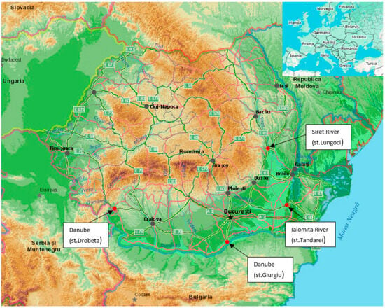
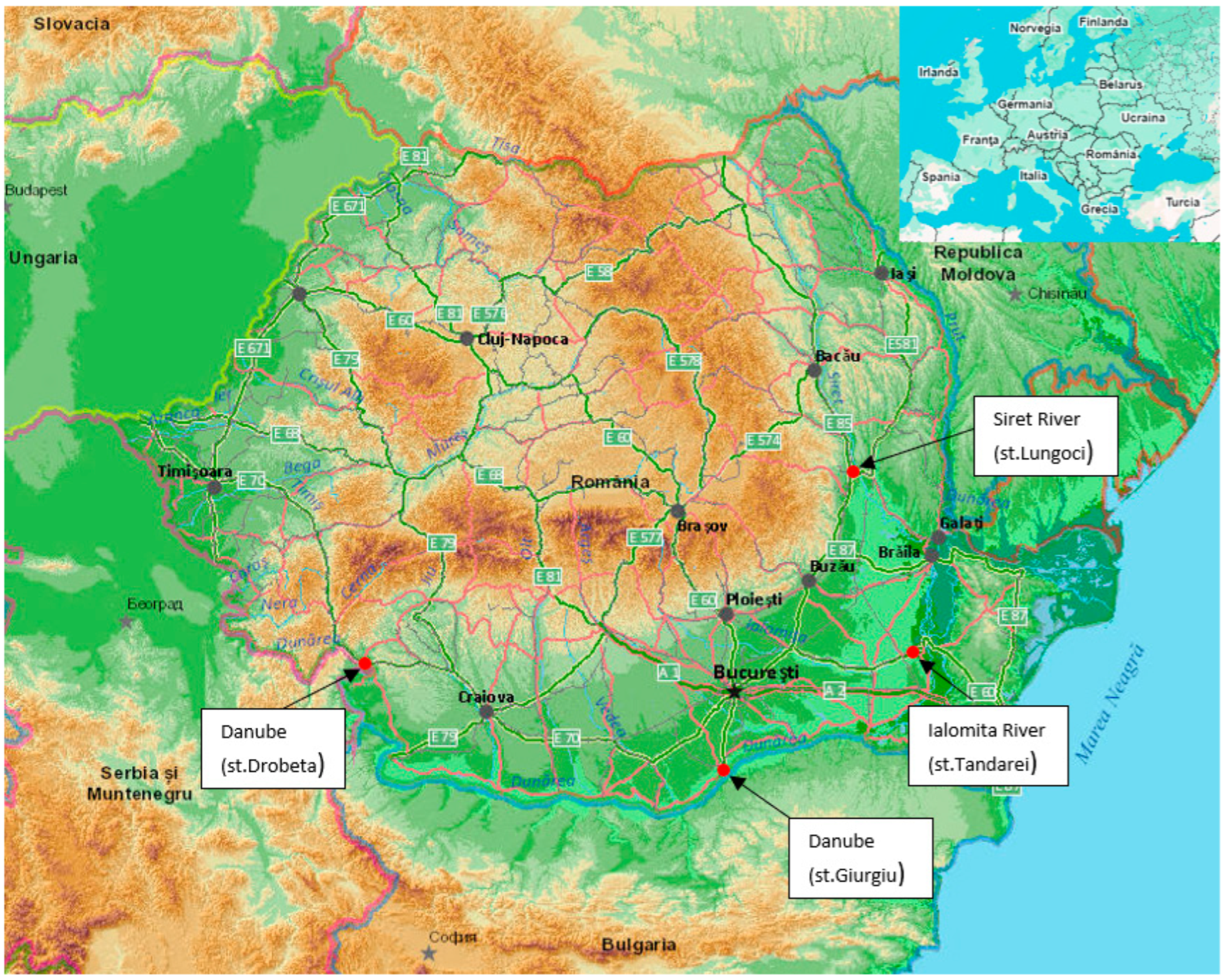
Figure 1 illustrates the four investigated locations considered in the analysis. Two of these sites are situated along the Danube River, reflecting the hydrological significance of this major transboundary watercourse, while one location is positioned on the Siret River and another on the Ialomița River. All selected gauging stations are located within Romania and were chosen to ensure a representative coverage of different hydroclimatic and physiographic conditions. This spatial distribution allows for a comparative assessment of hydrological behavior across distinct river basins, capturing both large lowland rivers and medium-sized catchments influenced by regional climatic variability.

Figure 1. Geographical distribution of the four hydrometric stations included in the analysis [14].

The hydrological analysis covers three major river systems in Romania, namely the Danube River, the Siret River, and the Ialomița River, which together represent a wide range of physiographic and hydroclimatic conditions.

The Danube, the second longest river in Europe with a length of about 2860 km, originates in the Black Forest Mountains and discharges into the Black Sea through the Danube Delta, crossing or bordering multiple countries, including Romania, where it extends for approximately 1075 km. Along its Romanian course, the river exhibits distinct geomorphological sectors, ranging from the narrow gorge reach between Baziaș and Drobeta-Turnu Severin, where the Iron Gates I and II hydropower schemes are located, to wide floodplain and deltaic reaches downstream, and its flow regime is controlled by both alpine and Carpathian snowmelt, as well as precipitation, with major tributaries such as the Cerna, Jiu, Olt, Argeș, Ialomița, and Siret contributing significantly to its discharge.

The Siret River, the largest Romanian tributary of the Danube in terms of catchment area (approximately 47,610 km²), originates in the Eastern Carpathians and flows for about 706 km, of which 559 km are on Romanian territory, being characterized by a nival–pluvial regime with pronounced spring floods driven by snowmelt and secondary peaks in autumn due to rainfall, a high flood potential, and a temperate-continental climate marked by strong spatial contrasts in temperature and precipitation between mountainous and lowland areas.

The Ialomița River, originating in the Bucegi Mountains at elevations of around 2300 m, drains a basin of about 10,350 km² over a length of roughly 417 km and exhibits a similar nival–pluvial regime, with maximum discharges in spring and frequent flood hazards in the plain sector, while low flows and drought conditions commonly occur during summer.

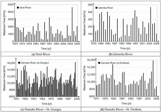
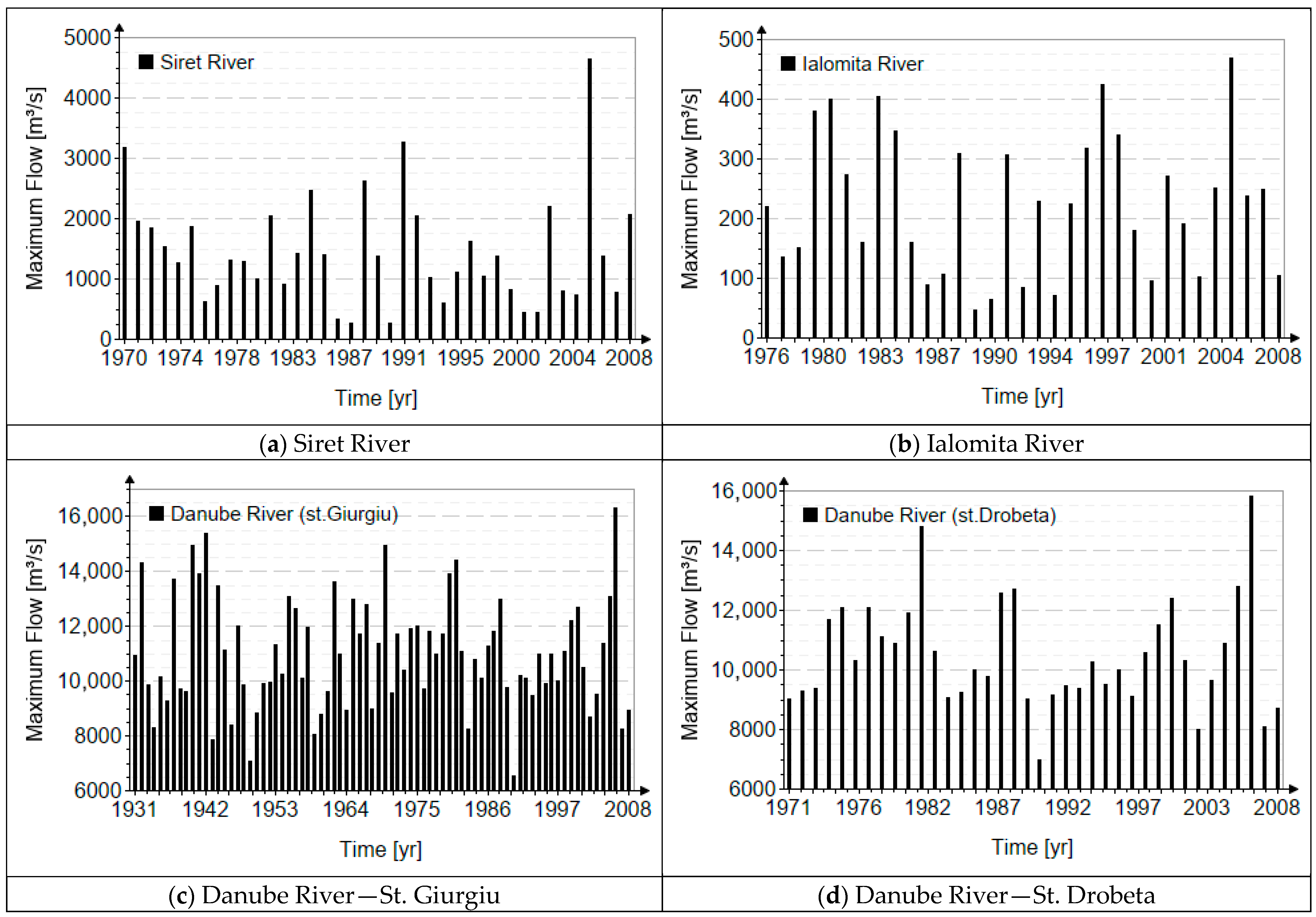
Figure 2 presents the chronological data series analyzed for each hydrometric station, providing the basis for subsequent statistical and frequency analyses.

Figure 2. The annual values of maximum discharges.

The record lengths of the analyzed hydrological series vary across the selected rivers and gauging stations, ensuring a representative temporal coverage for frequency analysis. For the Danube River, two stations are considered: Drobeta, with an observation record spanning 38 years, and Giurgiu, which provides a substantially longer series of 78 years, offering a robust basis for extreme-value assessment. The Siret River is represented by the Lungoci station, with a record length of 39 years, while the Ialomița River is analyzed by using data from the Tăndărei station, covering 33 years. These record lengths reflect both the availability of long-term observations and the relevance of the selected stations for hydrological design and regulatory applications.

The statistical indicators for the analyzed sites are summarized in Table 1.

Table 1. Statistical indicators of the observed data.

River/Station	$\mathit{\mu }$	${\mathit{C}}_{\mathit{v}}$	${\mathit{C}}_{\mathit{s}}$	${\mathit{C}}_{\mathit{s}}^{\mathit{c}\mathit{o}\mathit{r}\mathit{r}\mathit{e}\mathit{c}\mathit{t}\mathit{e}\mathit{d}}$	${\mathit{C}}_{\mathit{k}}$ (Kurtosis)
	[m3/s]	[-]	[-]	[-]	[-]
Siret/Lungoci	1442.5	0.634	0.379	1.269	7.872
Ialomita/Tandarei	224.1	0.527	0.327	1.054	4.074
Danube/Drobeta	10480.4	0.173	0.881	0.347	6.167
Danube/Giurgiu	10972.7	0.184	0.379	0.368	4.853

Where $\mu$ represents the arithmetic mean, $C_v$ is the coefficient of variation, and $C_s$ is the skewness coefficient.

The $C_s^{corrected}$ denotes the corrected skewness coefficient. Taking into account the relatively short lengths of the available data, the skewness was established according to Romanian practices: namely, multiplying the coefficient of variation by a factor $\xi$ that depends on the origin of the maximum flows. In both cases, the chosen coefficient is two. This coefficient reflects the dominant genesis of high flows, taking values of two for flows generated by snowmelt, three for flows generated by mixed sources (snowmelt and rainfall), and four for peak flows generated exclusively by rainfall.

To evaluate the temporal consistency of the hydrological record, a stationarity analysis was performed, using the t-test. The results indicate that the time series of annual maximum discharges does not exhibit statistically significant trends or systematic changes over the observation period, supporting the assumption of stationarity and confirming that the dataset is suitable for frequency analysis.

In addition, the Grubbs test was applied to identify potential anomalous or extreme values that could bias the statistical characterization of the series; however, no outliers were detected, confirming the homogeneity and overall reliability of the observed data.

4. Results and Discussions

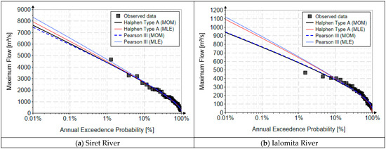
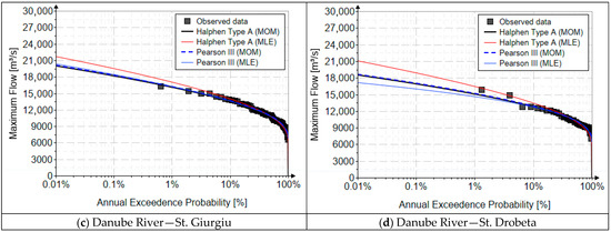
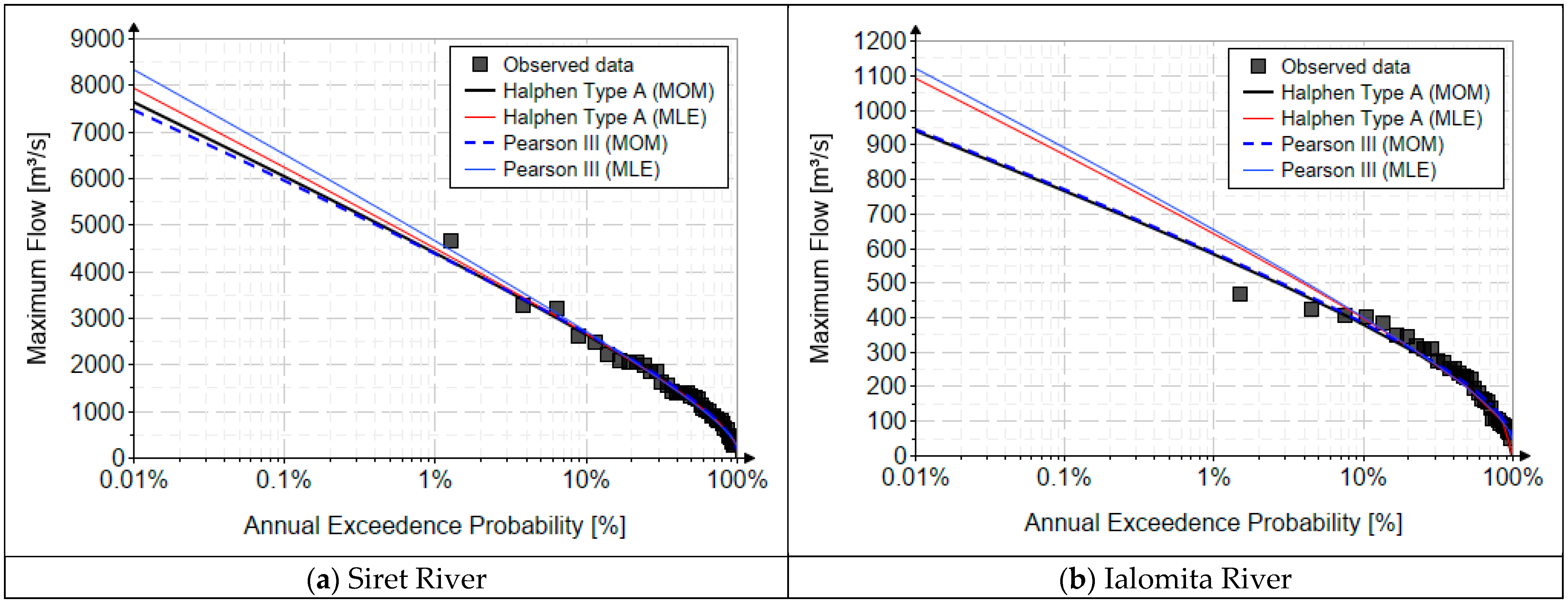
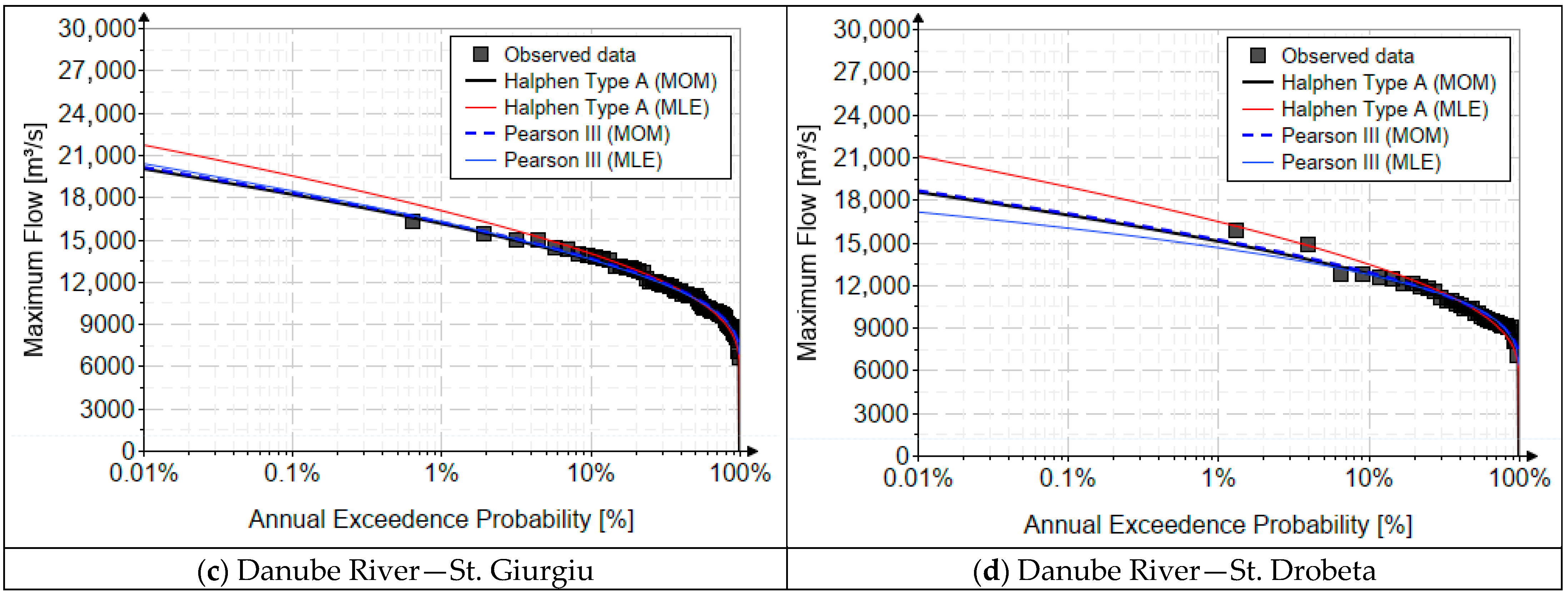
The comparative analysis between the Halphen-A and Pearson Type III distributions, as illustrated by the quantile plots in Figure 3, demonstrates that both models reproduce the observed annual maximum discharges with a high degree of numerical accuracy over the range of available data. However, the practical relevance of a flood frequency model is not determined primarily by its ability to interpolate moderate events, but rather by its capacity to extrapolate reliably toward long return periods, where the upper tail of the distribution dominates the design decisions.

Figure 3. The quantile function curves corresponding to the analyzed probability distribution.

The visual evidence shows that the relative differences between Halphen-A and Pearson III increase with the return period. This implies that, in relative terms, the discrepancy between the two models at T > 100 years is significantly larger than at T = 10 or 20 years. In hydrotechnical practice, such differences may easily reach several percent in peak discharge, which is far from negligible: a 5–10% difference in a 100-year or 1000-year flood can translate into substantial changes in spillway capacity, levee crest elevation, or floodplain inundation extent.

The graphical comparison reveals that for both the Siret and Ialomița rivers, the fitted curves are nearly indistinguishable at low and medium return periods (T < 50 years), where the empirical data are relatively dense and where most probability mass is concentrated. In this region, the differences between Halphen-A and Pearson III remain marginal and hydrologically insignificant. In contrast, for higher return periods (T > 100 years), the curves begin to diverge systematically, particularly in the upper tail, where the Halphen-A distribution produces smoother and more gradually increasing quantiles. This behavior indicates a reduced tail curvature compared with Pearson III, which tends to impose a more rigid extrapolation pattern, controlled primarily by the sample skewness.

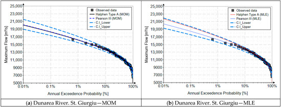
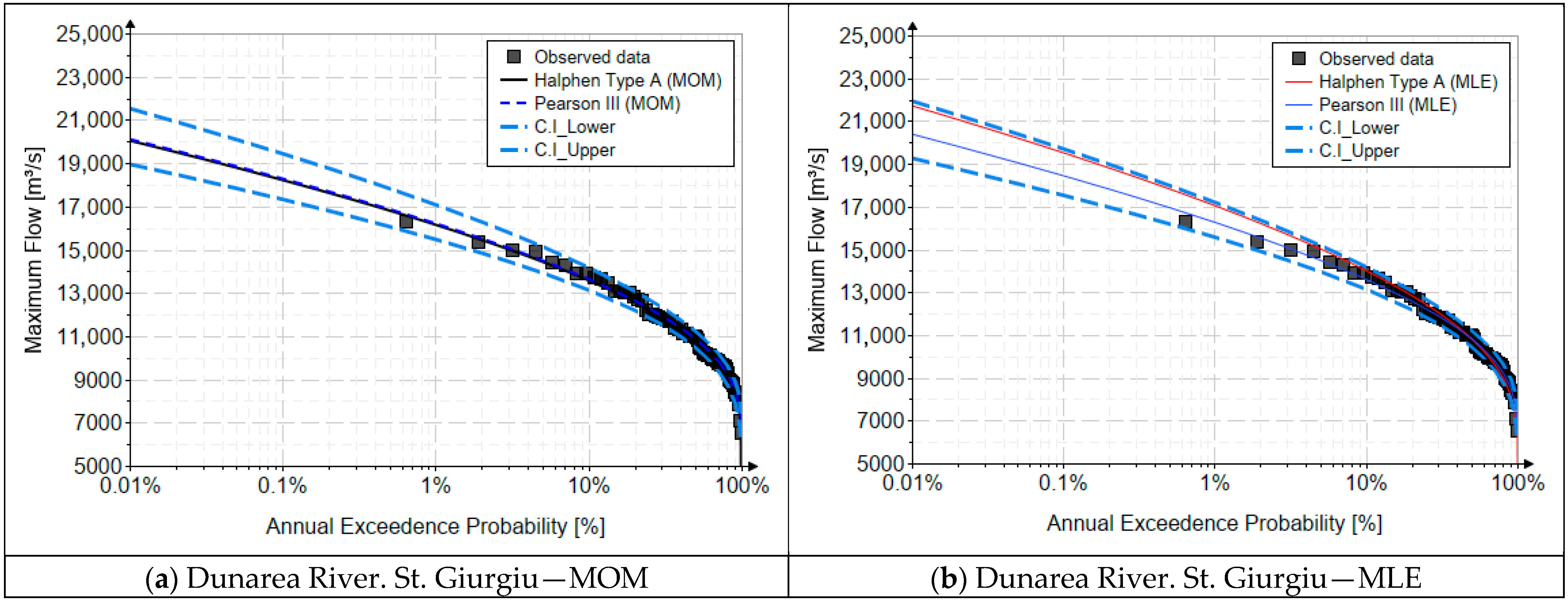
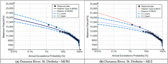
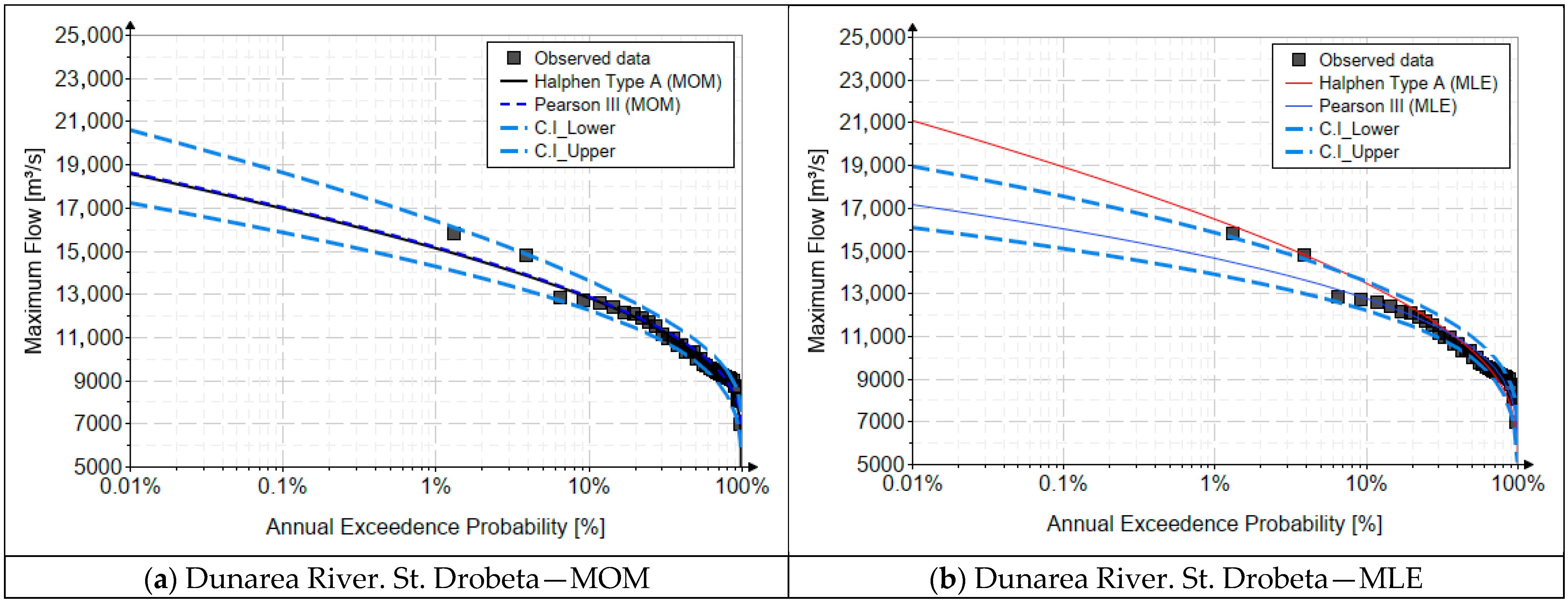
The results obtained for the Danube River at the Giurgiu and Drobeta stations highlight the inherent uncertainty associated with extrapolating flood quantiles toward very low annual exceedance probabilities. In the range of small probabilities (typically below 1%, corresponding to return periods greater than 100 years), the estimated discharges lie largely outside the domain of the observed data, which is limited by the finite record lengths. Under these conditions, the choice of both the probability distribution and the parameter-estimation method becomes decisive, as the fitted curves are no longer strongly constrained by empirical observations, but mainly by the assumed tail behavior of the model.

A consistent pattern can be observed when comparing the Halphen Type A and Pearson III distributions fitted using the MOM and MLE. In the upper tail, Halphen Type A generally yields higher quantile estimates than Pearson III, especially when parameters are estimated via MLE, indicating a heavier tail and a more conservative characterization of extreme floods. Differences between MOM and MLE are modest within the central probability range, where the data density is higher, but they become increasingly pronounced toward the lower exceedance probabilities, where small changes in parameter values translate into substantial differences in predicted peak flows.

Regarding the selection of the most appropriate model, performance indicators are commonly employed as objective evaluation criteria. Table 2, Table 3 and Table 4 present the resulting values of these indicators: namely, the RMSE (root mean square error) and MAE (mean absolute error). It should be noted that, by construction, these indicators primarily reflect the model’s goodness of fit within the range of the observed data, where empirical information is available and densely sampled.

Table 2. RMSE and MAE score values for the Ialomita River.

	Ialomita River
Distribution	MAE		RMSE
	MOM	MLE	MOM	MLE
Halphen-A	0.0404	0.0373	0.0085	0.008
Pearson III	0.0404	0.0383	0.0085	0.0082

Table 3. RMSE and MAE score values for the Siret River.

	Siret River
Distribution	MAE		RMSE
	MOM	MLE	MOM	MLE
Halphen-A	0.021	0.0224	0.00399	0.0042
Pearson III	0.0203	0.0278	0.00395	0.0052

Table 4. RMSE and MAE score values for the Danube River.

	Danube River—St. Giurgiu				Danube River—St. Drobeta
Distribution	MAE		RMSE		MAE		RMSE
	MOM	MLE	MOM	MLE	MOM	MLE	MOM	MLE
Halphen-A	0.0184	0.0266	0.0026	0.0036	0.0377	0.0536	0.0074	0.0105
Pearson III	0.0184	0.0174	0.0026	0.0025	0.0377	0.0448	0.0074	0.0089

Consequently, low RMSE and MAE values indicate a good overall agreement between the fitted distribution and the recorded annual maximum flows, particularly in the central and upper-probability domains that are well supported by observations. However, these metrics provide limited insight into the model behavior in the extreme lower exceedance probability range, where design-relevant quantiles are typically sought and where the estimated values lie outside the domain of the observed record.

Therefore, while RMSE and MAE are useful for identifying models that best reproduce the historical data, they should not be regarded as sufficient criteria for assessing the reliability of extrapolated extreme floods. A comprehensive model selection should also consider the theoretical properties of the distribution tail, the stability of parameter estimates, and the consistency of predicted quantiles at long return periods, especially when the results are used for flood risk management and hydraulic design.

For the Siret and Ialomita rivers, the lowest RMSE and MAE values correspond to Halphen-A estimated by MLE, indicating not only a better overall fit but also a more stable representation of extremes. In relative terms, the improvement over Pearson III is small for moderate events but becomes more meaningful in the tail, where Pearson III exhibits slightly larger deviations.

For the Danube River at the Giurgiu and Drobeta gauging stations, the magnitude of the indicators is relatively small, indicating that all tested models reproduce the observed annual maximum flows reasonably well within the range of available data. For the Giurgiu station, both distributions yield very similar performance. In terms of MAE, Pearson III with MLE shows the lowest value (0.0174), slightly outperforming both Halphen-A and Pearson III fitted with MOM (0.0184). A comparable pattern is observed for RMSE, where Pearson III–MLE (0.0025) marginally improves upon the MOM-based fits (0.0026). These differences, although numerically small, suggest a slightly better overall fit of Pearson III when parameters are estimated via MLE, particularly in capturing deviations across the observed data range. At the Drobeta station, the results show higher MAE and RMSE values compared to Giurgiu, reflecting a larger dispersion of observed floods and possibly a more complex hydrological response. Here, again, Pearson III consistently provides lower error values than Halphen-A for both estimation methods, with Pearson III–MLE yielding the best overall performance (MAE = 0.0448, RMSE = 0.0089). The comparison between MOM and MLE indicates that MLE generally improves the fit, especially for Pearson III, whereas Halphen-A exhibits a more noticeable increase in errors when switching from MOM to MLE. These results indicate that, according to classical goodness-of-fit metrics, Pearson III (particularly when estimated using MLE) offers the best agreement with the observed data at both Danube stations. However, it is essential to emphasize that RMSE and MAE predominantly assess the model performance within the domain of recorded floods. As such, while Pearson III–MLE appears to be statistically preferable, based on these indicators, this does not automatically guarantee superior reliability in extrapolating extreme quantiles associated with very low exceedance probabilities.

Therefore, the numerical ranking provided by Table 2, Table 3 and Table 4 should be complemented by an analysis of tail behavior and parameter stability when selecting the most appropriate model for design-level flood estimation.

Uncertainty Considerations

The results highlight a fundamental statistical issue: flood frequency models are highly sensitive to the joint behavior of skewness and kurtosis, especially when data records are short or when a few extreme events dominate the higher-order moments.

For the Siret and Ialomița, the series are characterized by relatively limited sample lengths and by pronounced tail heaviness. Under such conditions, classical moment-based estimators become increasingly unstable, because the third and fourth moments are strongly influenced by a small number of observations. This instability directly affects the Pearson III distribution, whose shape is tightly coupled to the sample skewness. The Halphen-A distribution mitigates this problem by introducing additional flexibility into the relationship between skewness and kurtosis. This allows it to adapt more smoothly to the empirical tail structure without forcing extreme quantiles to follow the rigid extrapolation imposed by Pearson III. As a result, Halphen-A produces quantile curves that are more physically plausible for very rare floods, particularly when T exceeds 100 years.

In the case of the Danube River, the analyzed data series can be considered to be relatively long, with record lengths of up to 78 years, which provides a solid empirical basis for frequency analysis and leads to a better agreement among the fitted statistical models.

Consequently, the differences between the adopted distributions and parameter estimation methods are less pronounced than in the case of short records, since the available data constrain the fitted curves more effectively over the range of observed values.

Nevertheless, despite the considerable length of the series, the results remain affected by non-negligible biases, particularly in the upper tail of the distribution, corresponding to low annual exceedance probabilities. These biases arise from the limited information on rare extreme events, sampling variability, and the inherent assumptions of the adopted statistical models, and they may still have a significant impact on the estimation of design discharges used in flood risk management and hydraulic design applications.

In general, MLE consistently provides better performance than MOM, reflecting its higher statistical efficiency. However, the effect of the estimation method is not uniform across the considered distributions. Pearson III exhibits a greater sensitivity to the choice of estimator, especially in the distribution tail, whereas Halphen-A shows comparatively more stable behavior. This pattern is consistent with theoretical expectations, as MOM is more susceptible to the influence of skewness, kurtosis, and record length, due to its direct dependence on higher-order sample moments. By contrast, likelihood-based approaches are less affected by these distortions, although they remain intrinsically dependent on the assumed form of the probability distribution. In general, a key limitation of three-parameter distributions is that parameter estimation methods based on statistical descriptors (MOM, L-moments, LH-moments, and K-moments) are intrinsically restricted to calibrating only three independent statistics. As a consequence, the fourth statistical descriptor, namely kurtosis (or its counterparts L-kurtosis and LH-kurtosis), cannot be explicitly matched. This limitation is particularly important in the analysis of extreme maximum events, since kurtosis exerts a strong control on tail heaviness and, implicitly, on the behavior of high quantiles. Proper calibration of this fourth-order characteristic is only possible when using distributions with at least four parameters, such as the Wakeby distribution. However, this increased flexibility comes at the cost of significantly more complex and computationally demanding parameter-estimation procedures, which often require elaborate numerical algorithms and careful convergence control.

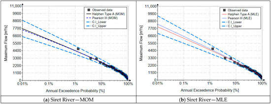
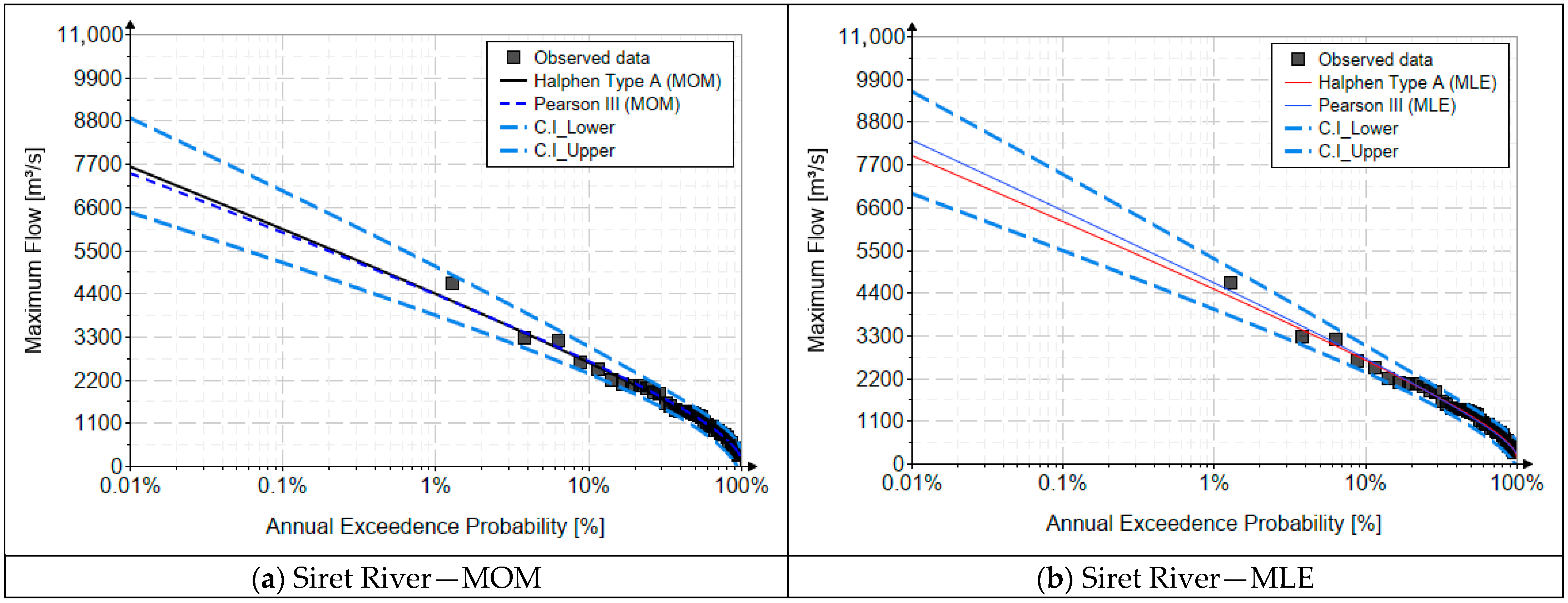
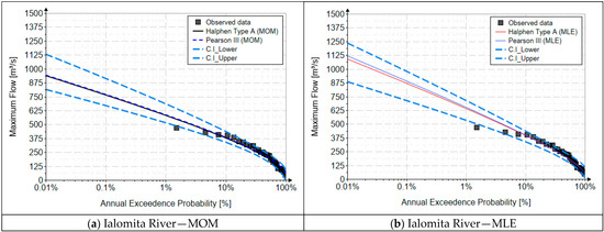
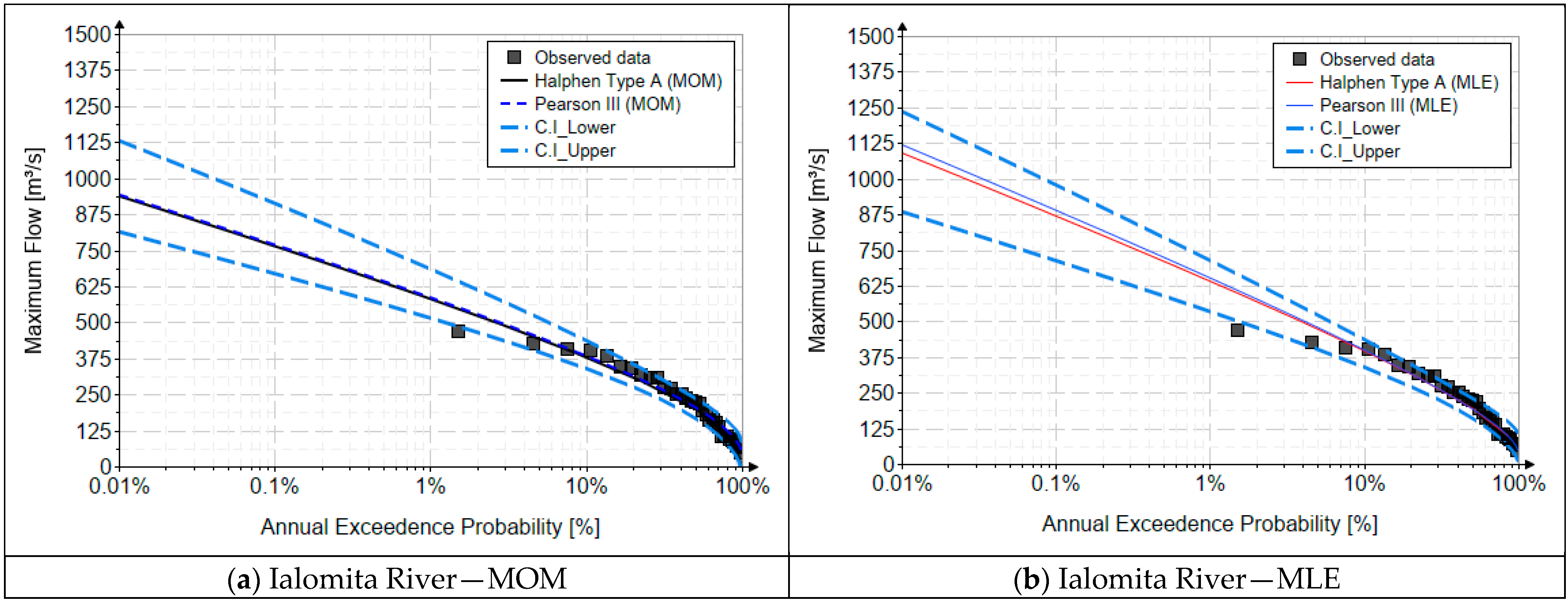
Considering that the Pearson type III distribution represents the reference distribution in Romanian hydrological practice for the analysis of annual maximum discharges, the plots shown in Figure 4, Figure 5, Figure 6 and Figure 7 are intended to highlight the uncertainty associated with quantile estimation and the degree of robustness of the statistical fit.

Figure 4. Confidence interval. Siret River.

Figure 5. Confidence interval. Ialomita River.

Figure 6. Confidence interval. Dunarea River—St. Giurgiu.

Figure 7. Confidence interval. Dunarea River—St. Drobeta.

In these graphical representations, the quantile curves estimated using the Pearson III distribution are presented together with the 95% confidence bands, constructed around the theoretical values. The confidence intervals reflect the variability induced by the record length, the parameter estimation method, and the distribution skewness, and therefore constitute a direct indicator of the uncertainty level of the predictions, particularly in the low-probability range corresponding to rare events.

By explicitly including confidence intervals, the figures provide a more rigorous interpretation than a simple comparison of theoretical curves, allowing for a simultaneous assessment of both the estimated value and the probable range within which it may vary. This approach is fully consistent with modern recommendations on uncertainty analysis in hydrology and supports the use of the Pearson III distribution, not only as a normative solution, but also as a statistically robust model that is capable of delivering coherent and interpretable estimates for hydrotechnical design and flood risk management.

5. Conclusions

The comparative flood frequency analysis performed for the Siret, Ialomița and Danube rivers leads to several technically significant conclusions that extend beyond simple goodness-of-fit metrics. While both the Halphen-A and Pearson Type III distributions provide satisfactory representations of the observed annual maximum discharges, their behavior diverges increasingly as the analysis moves toward high return periods, which are the most relevant for hydrotechnical design and flood risk management.

The results presented in Figure 3 and quantified through the RMSE and MAE values in Table 2, Table 3 and Table 4 demonstrate that Halphen-A, particularly when estimated by MLE, consistently yields the most stable and accurate fits. More importantly, the Halphen-A distribution produces smoother and more flexible upper-tail quantiles, which become increasingly distinct from those of Pearson III for T > 100 years. Although the two models are nearly equivalent in terms of frequent floods, their relative differences grow with the return period, implying that Pearson III may either over- or under-estimate extreme design floods when extrapolated far beyond the data range.

These differences are not merely statistical but have direct engineering implications. In the context of dam safety, flood protection works, and urban drainage systems, even a few percent difference in the estimated 100-year or 1000-year flood can determine whether a structure is overtopped, whether a spillway is undersized, or whether floodplain zoning is overly conservative or dangerously optimistic. The evidence from this study therefore suggests that Halphen-A offers a more reliable basis for high-return-period design in Romanian river basins characterized by strong skewness and heavy tails.

The analysis also confirms that parameter estimation methods play a critical role. The MLE systematically outperforms the MOM, especially for extreme quantiles, because it is less sensitive to the distortions introduced by skewness, kurtosis, and limited sample size. In contrast, MOM, which remains the parent method in Romanian practice, is inherently vulnerable to these effects, particularly when higher-order moments are dominated by a few large floods. This vulnerability propagates directly into Pearson III estimates, reinforcing the risk of biased tail extrapolation.

From a broader methodological perspective, these findings also point to the limitations of using MOM as the “parent method” in Romanian hydrological practice.

While MOM has the advantage of simplicity and long-standing tradition, it is not optimal for highly skewed, heavy-tailed, or short flood records, which are precisely the conditions encountered in many Romanian basins.

Rigorous alternatives such as L-moments [27,28,29] and, more recently, K-moments (knowable moments) [15,30,31] have been specifically developed to address these shortcomings by reducing sensitivity to outliers and improving robustness under limited data availability.

Unfortunately, these methods are not yet embedded in Romanian regulations, which still rely primarily on MOM-based Pearson III analyses.

In conclusion, this study provides strong empirical support for the integration of Halphen-type models, and particularly the Halphen-A distribution, into Romanian flood frequency analysis.

Used in combination with statistically efficient estimation methods, Halphen-A can reduce tail bias, improve the physical plausibility of extreme quantiles, and, ultimately, contribute to safer and more resilient hydrotechnical designs.

The findings also underscore the need for a gradual modernization of national standards [12], moving beyond traditional MOM-based Pearson III and toward more flexible and robust statistical frameworks that better reflect the realities of contemporary hydrology.

6. Future Directions

The analysis will focus on assessing the Halphen distribution under climate change and nonstationary conditions, where time-invariant parameters are no longer adequate. This includes developing nonstationary Halphen models with parameters linked to time or relevant climatic/hydrological covariates and benchmarking their performance against standard distributions, using information criteria and tail-oriented validation.

A Bayesian framework will be explored to improve parameter estimation and uncertainty quantification, allowing for the integration of prior information and the derivation of robust credible intervals for extreme quantiles. Additionally, recent approaches such as nonstationary POT/GP models, mixture or regime-switching models, and Bayesian model averaging will be investigated to better represent changing flood-generation mechanisms and reduce model uncertainty in design-flood estimation [32,33].

References

- Blöschl, G.; Hall, J.; Parajka, J.; Perdigão, R.A.P.; Merz, B.; Arheimer, B.; Aronica, G.T.; Bilibashi, A.; Bonacci, O.; Borga, M.; et al. Changing climate shifts timing of European floods. Science 2017, 357, 588–590. [Google Scholar] [CrossRef] [Scilit] [PubMed]
- Kundzewicz, Z.W.; Kanae, S.; Seneviratne, S.I.; Handmer, J.; Nicholls, N.; Peduzzi, P.; Mechler, R.; Bouwer, L.M.; Arnell, N.; Mach, K.; et al. Flood risk and climate change: Global and regional perspectives. Hydrol. Sci. J. 2013, 59, 6351. [Google Scholar] [CrossRef] [Scilit]
- Razi Ghalavand, M.; Farajzadeh, M.; Ghavidel Rahimi, Y. Modeling Return Levels of Non-Stationary Rainfall Extremes Due to Climate Change. Atmosphere 2025, 16, 136. [Google Scholar] [CrossRef] [Scilit]
- Papalexiou, S.M.; Montanari, A. Global and regional increase of precipitation extremes under global warming. Water Resour. Res. 2019, 55, 4901–4914. [Google Scholar] [CrossRef] [Scilit]
- Juan-Diego, E.; Mendoza, A.; Arganis-Juárez, M.L.; Berezowsky-Verduzco, M. Alteration of Catchments and Rivers, and the Effect on Floods: An Overview of Processes and Restoration Actions. Water 2025, 17, 1177. [Google Scholar] [CrossRef] [Scilit]
- Li, Y.; Rodriguez, F.; Berthier, E. Development and Evaluation of a Saturated Zone Module in an Integrated Urban Hydrological Model. Water 2022, 14, 1030. [Google Scholar] [CrossRef] [Scilit]
- Viglione, A.; Merz, R.; Salinas, J.L.; Blöschl, G. Flood frequency hydrology: 3. A Bayesian analysis. Water Resour. Res. 2013, 49, 675–692. [Google Scholar] [CrossRef] [Scilit]
- Merz, B.; Vorogushyn, S.; Lall, U.; Viglione, A.; Blöschl, G. Charting unknown waters—On the role of surprise in flood risk assessment and management. Water Resour. Res. 2015, 51, 6399–6416. [Google Scholar] [CrossRef] [Scilit]
- Lee, D.-H.; Kim, N.W. Regional Flood Frequency Analysis for a Poorly Gauged Basin Using the Simulated Flood Data and L-Moment Method. Water 2019, 11, 1717. [Google Scholar] [CrossRef] [Scilit]
- Khaliq, M.; Ouarda, T.; Ondo, J.-C.; Gachon, P.; Bobée, B. Frequency analysis of a sequence of dependent and/or non-stationary hydro-meteorological observations: A review. J. Hydrol. 2006, 329, 534–552. [Google Scholar] [CrossRef] [Scilit]
- Kundzewicz, Z.W.; Hirabayashi, Y.; Kanae, S. River Floods in the Changing Climate—Observations and Projections. Water Resour. Manag. 2010, 24, 2633–2646. [Google Scholar] [CrossRef] [Scilit]
- The Regulations Regarding the Establishment of Maximum Flows and Volumes for the Calculation of Hydrotechnical Retention Constructions; Ministry of Regional Development and Tourism: Bucharest, Romania, 2012.
- Anghel, C.-G.; Ianculescu, D. An In-Depth Statistical Analysis of the Pearson Type III Distribution Behavior in Modeling Extreme and Rare Events. Water 2025, 17, 1539. [Google Scholar] [CrossRef] [Scilit]
- Anghel, C.G.; Ianculescu, D. Application of the GEV Distribution in Flood Frequency Analysis in Romania: An In-Depth Analysis. Climate 2025, 13, 152. [Google Scholar] [CrossRef] [Scilit]
- Ianculescu, D.; Anghel, C.G. Innovative Explicit Relations for Weibull Distribution Parameters Based on K-Moments. Mathematics 2025, 13, 3473. [Google Scholar] [CrossRef] [Scilit]
- Anghel, C.G.; Ianculescu, D. Probabilistic Forecasting of Peak Discharges Using L-Moments and Multi-Parameter Statistical Models. Water 2025, 17, 1908. [Google Scholar] [CrossRef] [Scilit]
- El Adlouni, S.; Bernard, B. Halphen Distribution Family: With Application in Hydrological Frequency Analysis; Water Resources Publications: Littleton, CO, USA, 2017. [Google Scholar]
- Zhang, L.; Singh, V.P. Revisiting the Application of Halphen Distributions in Flood Frequency Analysis. J. Hydrol. Eng. 2021, 26, 04021042. [Google Scholar] [CrossRef] [Scilit]
- El Adlouni, S.; Chebana, F.; Bobée, B. Generalized Extreme Value versus Halphen System: Exploratory Study. J. Hydrol. Eng. 2010, 15, 79–89. [Google Scholar] [CrossRef] [Scilit]
- Dvorák, V.; Bobée, B.; Boucher, S.; Ashkar, F. Halphen Distributions and Related Systems of Frequency Functions; Rapport Scientifique (R236); INRS-Eau: Quebec City, QC, Canada, 1988. [Google Scholar]
- Perreault, L.; Bobée, B.; Rasmussen, P.F. Halphen Distribution System. I: Mathematical and Statistical Properties. J. Hydrol. Eng. 1999, 4, 189–199. [Google Scholar] [CrossRef]
- Salinas, J.L.; Castellarin, A.; Viglione, A.; Kohnová, S.; Kjeldsen, T.R. Regional parent flood frequency distributions in Europe—Part 1: Is the GEV model suitable as a pan-European parent? Hydrol. Earth Syst. Sci. 2014, 18, 4381–4389. [Google Scholar] [CrossRef] [Scilit]
- Bulletin 17B Guidelines for Determining Flood Flow Frequency; Hydrology Subcommittee, Interagency Advisory Committee on Water Data. U.S. Department of the Interior, U.S. Geological Survey, Office of Water Data Coordination: Reston, VA, USA, 1981.
- Mason, R.R., Jr. Bulletin 17C Guidelines for Determining Flood Flow Frequency; U.S. Department of the Interior, U.S. Geological Survey: Reston, VA, USA, 2017.
- Papalexiou, S.M.; Koutsoyiannis, D. Battle of extreme value distributions: A global survey on extreme daily rainfall. Water Resour. Res. 2013, 49, 187–201. [Google Scholar] [CrossRef] [Scilit]
- Coles, S.; Pericchi, L.R.; Sisson, S. A fully probabilistic approach to extreme rainfall modeling. J. Hydrol. 2003, 273, 35–50. [Google Scholar] [CrossRef] [Scilit]
- Rao, A.R.; Hamed, K.H. Flood Frequency Analysis; CRC Press: Boca Raton, FL, USA, 2000; ISBN 978-0-8493-0083-7. [Google Scholar]
- H Hosking, J.R.M.; Wallis, J.R. Regional Frequency Analysis, An Approach Based on L-Moments; Cambridge University Press, The Edinburgh Building: Cambridge, UK, 1997; ISBN 13-978-0-521-43045-6. [Google Scholar]
- Hosking, J.R.M. L-Moments: Analysis and Estimation of Distributions Using Linear Combinations of Order Statistics. J. R. Stat. Soc. 1990, 52, 105–124. [Google Scholar] [CrossRef] [Scilit]
- Koutsoyiannis, D. Knowable moments for high-order stochastic characterization and modelling of hydrological processes. Hydrol. Sci. J. 2019, 64, 19–33. [Google Scholar] [CrossRef] [Scilit]
- Koutsoyiannis, D. Knowable Moments in Stochastics: Knowing Their Advantages. Axioms 2023, 12, 590. [Google Scholar] [CrossRef] [Scilit]
- Xu, W.; Jiang, C.; Yan, L.; Li, L.; Liu, S. An Adaptive Metropolis-Hastings Optimization Algorithm of Bayesian Estimation in Non-Stationary Flood Frequency Analysis. Water Resour. Manag. 2018, 32, 1343–1366. [Google Scholar] [CrossRef] [Scilit]
- Li, L.; Krasovskaia, I.; Xiong, L.; Yan, L. Analysis and projection of runoff variation in three Chinese rivers. Hydrol. Res. 2017, 48, 1296–1310. [Google Scholar] [CrossRef] [Scilit]
Disclaimer/Publisher’s Note: The statements, opinions and data contained in all publications are solely those of the individual author(s) and contributor(s) and not of MDPI and/or the editor(s). MDPI and/or the editor(s) disclaim responsibility for any injury to people or property resulting from any ideas, methods, instructions or products referred to in the content. |
© 2026 by the authors. Licensee MDPI, Basel, Switzerland. This article is an open access article distributed under the terms and conditions of the Creative Commons Attribution (CC BY) license.