Joint Covariate Balancing for Difference-in-Differences with Missing Outcome Evolutions

Abstract

We propose a joint covariate balancing estimator for the average treatment effect on the treated (ATT) in a difference-in-differences (DID) design when the outcome evolution, rather than a specific outcome level, is missing at random (MAR). The proposed estimator combines treatment and response into one indicator and calibrates the two group-based density ratios directly. Point estimation therefore requires only two nuisance working models, and inference adds two linear projections, giving four in total, whereas a factorized implementation of the efficient influence function requires five: one treatment probability, two response probabilities, and two outcome-evolution models. The estimator is automatically self-normalized and attains the semiparametric efficiency bound for the coarsened data model when all working models are correctly specified. Furthermore, we show that the proposed estimator is doubly robust for both consistency and inference. The simulation results support componentwise robustness and confirm the efficiency result when all nuisance models are correctly specified, while highlighting substantial small-sample limitations under low response probabilities. An all-correct design further shows that the efficiency ordering relative to an estimator using the always-observed outcome level can reverse.

1. Introduction

Semiparametric difference-in-differences (DID) estimators adjust for differences in pre-treatment covariates when parallel trends hold conditionally rather than unconditionally (Abadie, 2005; Sant’Anna & Zhao, 2020). In practice, however, the outcome is often missing for some units, and a simple complete-case analysis that discards all units with any missing outcome is inefficient, and is biased whenever response depends on covariates that also shift the outcome evolution. To address this issue, researchers have developed methods assuming that outcomes are missing at random (MAR) (Tang et al., 2024; Tsiatis, 2006; A. Zhao et al., 2024). In DID with MAR, Testa et al. (2026) propose a semiparametric DID estimator based on the efficient influence function (EIF) of the ATT to enhance efficiency. However, this construction introduces several nuisance models that must all be correctly specified to attain the semiparametric efficiency bound, which is challenging in practice. Reducing the number of nuisance models in the MAR DID setting is therefore desirable, though it is not obvious how to achieve this. The covariate balancing propensity score (CBPS) framework (Fan et al., 2023; Imai & Ratkovic, 2014; Li & Matsushita, 2025) provides this possibility, as it allows the composite of the treatment and response probabilities, namely, the group-based density ratio, to be calibrated directly in a single step.

In this paper, we propose a joint covariate balancing estimator for the ATT in a DID design with outcomes missing at random. The proof architecture for double robustness in DID follows Sant’Anna and Zhao (2020), and the calibration machinery follows the covariate balancing literature (Fan et al., 2023; Imai & Ratkovic, 2014) and its complete-data DID implementation (Li & Matsushita, 2025). Two elements are new. First, we coarsen the outcome to its evolution and combine treatment and response into a single indicator, so that the missingness restriction is placed on the outcome evolution rather than on a particular outcome level; the efficient influence function of the resulting observed-data model is derived in Proposition 1, and Remark 1 quantifies the efficiency consequence of the coarsening. Second, the calibration condition is joint across the two respondent groups, estimates the two group-based density ratios directly, and uses the treated sample as the common balancing target.

These two choices deliver the three properties that constitute our contribution. First, the proposed DID estimator reduces the number of nuisance models required, using only two working models for point estimation where a factorized implementation would require five, without losing local efficiency (i.e., it attains the semiparametric efficiency bound), and it is automatically self-normalized (i.e., it has the Hájek form). Inference additionally uses the two weighted least-squares projections, so that four working models enter in total, against five in the factorized implementation. Second, the proposed DID estimator is componentwise doubly robust for consistency: it is consistent if, for each respondent group, at least one of the density-ratio model and the outcome-evolution model is correctly specified. Third, the proposed DID estimator has a form-invariant asymptotic variance as long as, for each respondent group, at least one of the density-ratio model and the outcome-evolution model is correctly specified, a property known as double robustness for inference. Our numerical study examines small-sample inference, both favorable and unfavorable working-model configurations, and the efficiency comparison with an outcome-level estimator.

The estimator also sits within a broader literature on balancing and calibration weights. Inverse probability tilting (Graham et al., 2012) and entropy balancing (Hainmueller, 2012) construct weights by exponential tilting subject to moment constraints; Q. Zhao and Percival (2017) show that entropy balancing is doubly robust, and Chan et al. (2016) establish global efficiency for empirical balancing calibration weighting with a growing dictionary. Related constructions include stable balancing weights (Zubizarreta, 2015), kernel-based covariate functional balancing (Wong & Chan, 2018), and tailored loss functions (Q. Zhao, 2019). Our joint balancing condition inherits from this literature the exponential-tilting form of the weights, the exact finite-sample moment matching, and the convexity of the calibration problem. What is new is that the balancing target is the treated sample for both respondent groups simultaneously, and that each set of weights calibrates a composite of a treatment probability and a response probability rather than a single selection probability. On the missing-data side we rely on the coarsened data framework of Robins et al. (1994), Bang and Robins (2005) and Tsiatis (2006), and on the efficiency side on Hahn (1998) and Hirano et al. (2003). Finally, reducing the number of nuisance models is complementary to, rather than a substitute for, debiased machine learning (Chernozhukov et al., 2018).

The rest of the paper is organized as follows. Section 2 introduces the setup and assumptions. Section 3 derives the efficient influence function for the ATT and the associated componentwise doubly robust estimand. Section 4 presents the joint covariate balancing estimator. Section 5 establishes its local efficiency and its double robustness for both consistency and inference. Section 6 reports the Monte Carlo results. Section 7 concludes.

2. Setup

There are two periods, $t\in \{0,1\}$, and treatment starts only at $t=1$. Let $D\in \{0,1\}$ indicate treatment, $Y_t\left(d\right)$ denote potential outcomes, and $\Delta Y=Y_1-Y_0$. The indicator R equals one when both outcome levels needed for $\Delta Y$ are observed. The coarsened data are i.i.d. copies of $O=(X,D,R,R\Delta Y)$, where X is a fully observed vector of pre-treatment covariates. The parameter of interest is the ATT, defined as

$$\tau =\mathbb{E}[Y_1\left(1\right)-Y_1\left(0\right)\mid D=1].$$

(1)

Define $p=\mathbb{P}(D=1)$, $e^{*}\left(x\right)=\mathbb{P}(D=1\mid X=x)$, $r_d^{*}\left(x\right)=\mathbb{P}(R=1\mid D=d,X=x)$, $m_d^{*}\left(x\right)=\mathbb{E}(\Delta Y\mid D=d,X=x)$, $S_1=DR$, and $S_0=(1-D)R$. Write $a_d^{*}\left(x\right)=\mathbb{P}(S_d=1\mid X=x)$, so that

$$a_1^{*}\left(x\right)=e^{*}\left(x\right)r_1^{*}\left(x\right),a_0^{*}\left(x\right)=\{1-e^{*}\left(x\right)\}{r}_0^{*}\left(x\right).$$

(2)

The joint indicator is therefore multiplicative: each $a_d^{*}$ is a product of two probabilities. Next, we introduce the identification conditions for the ATT and the MAR conditions for the outcome evolution.

Assumption 1 (Identification conditions).

The following conditions hold:

 (i) 

$Y_1=D{Y}_1\left(1\right)+(1-D)Y_1\left(0\right)$ and $Y_0=Y_0\left(0\right)$ almost surely;

 (ii) 

$\mathbb{E}[Y_1\left(0\right)-Y_0\left(0\right)\mid D=1,X]=\mathbb{E}[Y_1\left(0\right)-Y_0\left(0\right)\mid D=0,X]$ almost surely;

 (iii) 

For some $\epsilon >0$, $p>\epsilon$ and $e^{*}\left(X\right)\le 1-\epsilon$ almost surely.

Assumption 1(i) imposes consistency and no anticipation: the observed post-treatment outcome agrees with the potential outcome under the realized treatment status, while the baseline outcome is untreated for every unit. Assumption 1(ii) is conditional parallel trends, which restricts the conditional mean of the untreated outcome evolution rather than the levels of the potential outcomes. Assumption 1(iii) is ATT overlap: treatment occurs with positive probability, and comparison units remain available over the covariate support relevant to the treated population. These conditions are standard in semiparametric DID analyses of the ATT (Abadie, 2005; Li & Matsushita, 2025; Sant’Anna & Zhao, 2020).

Assumption 2 (Missing at random and response overlap).

For each $d\in \{0,1\}$,

 (i) 

$R\perp \perp \Delta Y\mid (D=d,X)$;

 (ii) 

For some $\underline{r}>0$, $r_d^{*}\left(X\right)\ge \underline{r}$ almost surely on the covariate support of treated units.

Assumption 2(i) is an MAR restriction on observability of the outcome evolution, not a pair of date-specific MAR restrictions as imposed in Testa et al. (2026). It allows $R=0$ to arise from a missing baseline, a missing follow-up, or simultaneous missingness. If $Y_0$ is always observed, R is the post-treatment response indicator; if $Y_1$ is always observed, it is the pre-treatment response indicator. When either outcome may be missing, R is the complete-pair indicator, i.e., $R=R_0{R}_1$, where $R_t=\mathbf{1}\left\{Y_t\mathrm{observed}\right\}$ for $t\in \{0,1\}$.

Example 1.

Assumption 2(i) restricts only outcome evolution, so it is useful to clarify the forms of dependence between R and the outcome levels $(Y_0,Y_1)$ that it permits. For example, suppose that for some measurable h and some unobserved U,

$$R=h(X,D,Y_0,U),U\perp \perp (Y_0,\Delta Y)\mid (D,X),Y_0\perp \perp \Delta Y\mid (D,X).$$

(3)

Clearly, $(Y_0,U)\perp \perp \Delta Y\mid (D,X)$ implies $R\perp \perp \Delta Y\mid (D,X)$, so Assumption 2(i) holds. However, since R is a nondegenerate function of the baseline outcome $Y_0$ and $Y_1=Y_0+\Delta Y$, neither of the date-specific conditions $Y_0\perp \perp R\mid (D,X)$ and $Y_1\perp \perp R\mid (D,X)$ need hold. An empirical example is missingness driven by the baseline outcome level: workers with low baseline earnings are more likely to be nonrespondents in a population where, conditional on age, education, and gender, baseline earnings carry no information about subsequent outcome evolution. In this setting, Assumption 2(i) accommodates mechanisms that are missing not at random (MNAR) with respect to the specific outcome levels, that is, $Y_0\cancel{⫫}R\mid (D,X)$ and $Y_1\cancel{⫫}R\mid (D,X)$.

More importantly, under Assumption 2(i), one can use the observed data to identify the conditional mean of the outcome evolution for each treatment group, i.e., $\mathbb{E}(\Delta Y\mid D=d,R=1,X)=\mathbb{E}(\Delta Y\mid D=d,X),d\in \{0,1\}$. Finally, under Assumptions 1–2, the ATT is identified by

$$\tau ={\displaystyle \frac{1}{p}}\mathbb{E}\left[\{S_1{\omega }_1^{*}\left(X\right)-S_0{\omega }_0^{*}\left(X\right)\}\Delta Y\right],$$

(4)

where

$${\omega }_1^{*}\left(x\right)={\displaystyle \frac{e^{*}\left(x\right)}{a_1^{*}\left(x\right)}}={\displaystyle \frac{1}{r_1^{*}\left(x\right)}},{\omega }_0^{*}\left(x\right)={\displaystyle \frac{e^{*}\left(x\right)}{a_0^{*}\left(x\right)}}={\displaystyle \frac{e^{*}\left(x\right)}{\{1-e^{*}\left(x\right)\}{r}_0^{*}\left(x\right)}}$$

(5)

are the group-based density ratios. The role of Assumption 2(ii) is now transparent: by (2) the denominator of ${\omega }_d^{*}=e^{*}/a_d^{*}$ is a product of two probabilities, so overlap in treatment alone does not keep the weights bounded. Identification itself only requires $a_d^{*}\left(X\right)>0$ on the covariate support of treated units, but Assumptions 1(iii) and 2(ii) are needed jointly to bound the weights. This identification result extends the inverse probability weighting (IPW) representation of Abadie (2005), in which only $e^{*}$ enters, to outcome evolutions that are missing at random. When outcomes are fully observed, (4) reduces to that representation. The proof is given in Appendix A.1.

3. Efficient Influence Function and Componentwise Doubly Robust Estimation

Before introducing the proposed estimator, we characterize the efficiency benchmark under the outcome evolution MAR condition.

Proposition 1 (Efficient influence function).

Under Assumptions 1–2, the efficient influence function for τ in the nonparametric model for $O=(X,D,R,R\Delta Y)$ is

$$\begin{array}{cc}\hfill {\phi }_{\mathrm{eff}}\left(O\right)=& {\displaystyle \frac{1}{p}}[S_1{\omega }_1^{*}\left(X\right)\{\Delta Y-m_1^{*}\left(X\right)\}-S_0{\omega }_0^{*}\left(X\right)\{\Delta Y-m_0^{*}\left(X\right)\}\hfill \\ \hfill & +D\{m_1^{*}\left(X\right)-m_0^{*}\left(X\right)-\tau \}],\hfill \end{array}$$

(6)

which satisfies $\mathbb{E}\left[{\phi }_{\mathrm{eff}}\left(O\right)\right]=0$, and $V_{\mathrm{eff}}=\mathbb{E}[{\phi }_{\mathrm{eff}}{\left(O\right)}^2]$ is the semiparametric efficiency bound for regular estimators of τ. When the outcome evolution is fully observed, that is, $r_1^{*}\left(X\right)=r_0^{*}\left(X\right)=1$ almost surely so that $R=1$ for all units, ${\phi }_{\mathrm{eff}}\left(O\right)$ reduces to the efficient influence function for the ATT with fully observed panel data derived in Sant’Anna and Zhao (2020). The proof is given in Appendix A.2.

Remark 1.

Proposition 2.8 of Testa et al. (2026) derives the efficient influence function for the ATT when the post-treatment outcome $Y_1$ is always observed and only the baseline outcome $Y_0$ may be missing. Their setting differs from ours in two respects. First, the MAR conditions differ. Their MAR condition is date-specific, requiring $Y_0\perp \perp R\mid (D,X)$ (their Assumption 2.3), whereas Assumption 2(i) imposes a single restriction on the observability of the outcome evolution $\Delta Y$ while allowing either outcome level, or both, to be missing. Hence, Assumption 2(i) is not nested within their date-specific restriction, nor is theirs nested within ours. Second, the observed data differ: in their setting, units with $R=0$ still contribute their post-treatment outcomes, whereas under our coarsening $O=(X,D,R,R\Delta Y)$ they contribute only $(X,D,R)$. To compare the efficiency bounds implied by the two MAR conditions, we work within the intersection of the two non-nested conditions by imposing the joint restriction

$$(Y_0,Y_1)\perp \perp R\mid (D,X),$$

(7)

which implies both their date-specific condition $Y_0\perp \perp R\mid (D,X)$ and our Assumption 2(i). Specializing our setup to theirs, so that R indicates whether $Y_0$ is observed, let ${\phi }_T$ denote their efficient influence function and let $V_{\mathrm{eff}}^T=\mathbb{E}\left({\phi }_T^2\right)$ denote the corresponding semiparametric efficiency bound for the observed data $O^T=(X,D,Y_1,R,R{Y}_0)$. Under the intersection condition (7), their efficient influence function can then be written as ${\phi }_T\left(O^T\right)={\phi }_{\mathrm{eff}}\left(O\right)+\Delta (O,Y_1)$, where

$$\Delta (O,Y_1)={\displaystyle \frac{D}{p}}\left\{1-{\displaystyle \frac{R}{r_1^{*}\left(X\right)}}\right\}\{Y_1-{\nu }_1^{*}\left(X\right)\}-{\displaystyle \frac{(1-D)e^{*}\left(X\right)}{p\{1-e^{*}\left(X\right)\}}}\left\{1-{\displaystyle \frac{R}{r_0^{*}\left(X\right)}}\right\}\{Y_1-{\nu }_0^{*}\left(X\right)\},$$

(8)

is the adjustment that exploits the post-treatment outcomes of nonrespondents; here, ${\nu }_d^{*}\left(X\right)=\mathbb{E}(Y_1\mid D=d,X)$, and $\Delta (O,Y_1)$ is not a function of O. Under the intersection condition (7), straightforward algebra yields the following expression for the efficiency comparison:

$$V_{\mathrm{eff}}^T=V_{\mathrm{eff}}-{\displaystyle \frac{1}{p^2}}{\displaystyle \sum _{d=0}^1}\mathbb{E}\left[q_d^{*}\left(X\right)\{{\sigma }_{\Delta ,d}^{*2}\left(X\right)-{\sigma }_{0,d}^{*2}\left(X\right)\}\right],$$

(9)

where ${\sigma }_{\Delta ,d}^{*2}\left(X\right)=Var(\Delta Y\mid D=d,X)$, ${\sigma }_{0,d}^{*2}\left(X\right)=Var(Y_0\mid D=d,X)$, and the nonnegative weights are

$$q_1^{*}\left(X\right)={\displaystyle \frac{e^{*}\left(X\right)\{1-r_1^{*}\left(X\right)\}}{r_1^{*}\left(X\right)}},q_0^{*}\left(X\right)={\displaystyle \frac{e^{*}{\left(X\right)}^2\{1-r_0^{*}\left(X\right)\}}{\{1-e^{*}\left(X\right)\}{r}_0^{*}\left(X\right)}}.$$

The efficiency ranking can therefore go in either direction, depending on the serial dependence of the outcome. Writing ${\sigma }_{1,d}^{*2}\left(X\right)=Var(Y_1\mid D=d,X)$ and ${\sigma }_{\Delta ,d}^{*2}={\sigma }_{0,d}^{*2}+{\sigma }_{1,d}^{*2}-2{\rho }_d^{*}{\sigma }_{0,d}^{*}{\sigma }_{1,d}^{*}$ with ${\rho }_d^{*}$ the conditional correlation between $Y_0$ and $Y_1$ given $(D=d,X)$, the coarsened bound $V_{\mathrm{eff}}$ is the smaller of the two whenever ${\sigma }_{\Delta ,d}^{*2}<{\sigma }_{0,d}^{*2}$. For example, if ${\sigma }_{1,d}^{*}={\sigma }_{0,d}^{*}$, then ${\rho }_d^{*}>1/2$ implies $V_{\mathrm{eff}}<V_{\mathrm{eff}}^T$. In panel settings in which DID is typically applied, outcomes tend to exhibit strong serial correlation. Thus, coarsening the observed data to O and imposing Assumption 2(i) can be more, rather than less, informative than observing $Y_1$ for nonrespondents under the date-specific MAR condition. The ranking is reversed when the outcome evolution is more variable than the baseline outcome. The proof of (9) is provided in Appendix A.3.

In terms of the underlying conditional probabilities, $S_1{\omega }_1^{*}\left(X\right)=DR/r_1^{*}\left(X\right)$ and $S_0{\omega }_0^{*}\left(X\right)=(1-D)R{e}^{*}\left(X\right)/\left[\{1-e^{*}\left(X\right)\}{r}_0^{*}\left(X\right)\right]$, so (6) involves the three probability models $e^{*}$, $r_1^{*}$, and $r_0^{*}$, together with the two outcome-evolution models $m_1^{*}$ and $m_0^{*}$. Motivated by Equation (6), let ${\omega }_d\left(X\right)$ and $m_d\left(X\right)$ denote working models for the group-based density ratio ${\omega }_d^{*}\left(X\right)$ and the outcome evolution $m_d^{*}\left(X\right)$, either of which may be misspecified, and define the augmented estimand

$${\tau }_{\mathrm{dr}}={\displaystyle \frac{1}{p}}\mathbb{E}\left[D\{m_1\left(X\right)-m_0\left(X\right)\}+S_1{\omega }_1\left(X\right)\{\Delta Y-m_1\left(X\right)\}-S_0{\omega }_0\left(X\right)\{\Delta Y-m_0\left(X\right)\}\right].$$

(10)

Proposition 2 (Componentwise double robustness).

Under Assumptions 1–2, ${\tau }_{\mathrm{dr}}=\tau$ if, for each $d\in \{0,1\}$, either ${\omega }_d\left(X\right)={\omega }_d^{*}\left(X\right)$ or $m_d\left(X\right)=m_d^{*}\left(X\right)$ almost surely.

Proposition 2 shows that the augmented estimand equals the ATT as long as, for each respondent group, at least one of the two working models is correctly specified. Modeling the weights through the two density ratios rather than the three probabilities also weakens the requirements: ${\omega }_1$ is correctly specified if and only if $r_1$ is, while ${\omega }_0$ is correctly specified whenever e and $r_0$ both are, but also under compensating misspecification of the two. Nevertheless, a factorized implementation of ${\tau }_{\mathrm{dr}}$ would still fit the three probability models separately and combine them, so that five working models enter in total. The proof is given in Appendix A.4.

Recall that while the efficient influence function involves the outcome-evolution models, the identification result (4) involves only the weighting functions. It is therefore worth exploiting this lower-nuisance identification while retaining the double robustness property. The joint covariate balancing approach of the next section calibrates the two group-based density ratios in (5) directly and dispenses with the separate estimation of $e^{*}$, $r_1^{*}$, and $r_0^{*}$; in addition, no outcome-evolution model $m_d^{*}\left(X\right)$ needs to be estimated for point estimation. Furthermore, the resulting estimator retains componentwise double robustness.

4. Joint Covariate Balancing Estimator

Let $b\left(X\right)={(1,b_2\left(X\right),\dots ,b_K\left(X\right))}^{\top }$ be a fixed dictionary. For each respondent group, consider a single-index working family generated by a scalar link function $g_d:\mathbb{R}\to (0,\infty )$ that is positive and twice continuously differentiable, with ${\dot{g}}_d\left(u\right)>0$ for every $u\in \mathbb{R}$,

$${\omega }_d(X;{\lambda }_d)=g_d\left\{b{\left(X\right)}^{\top }{\lambda }_d\right\},{\lambda }_d\in {\Lambda }_d\subset {\mathbb{R}}^K,d\in \{0,1\},$$

these conditions on the link are also collected in Assumption 3(ii) below. To distinguish the three roles associated with ${\omega }_d$, we use $g_d$ for the scalar link function, ${\omega }_d(·;{\lambda }_d)$ for the density-ratio working model induced by the link, and ${\omega }_d^{*}$ for the true group-specific density ratio. The derivative with respect to ${\lambda }_d$ takes the convenient form $\partial g_d\left\{b{\left(X\right)}^{\top }{\lambda }_d\right\}/\partial {\lambda }_d={\dot{g}}_d\left\{b{\left(X\right)}^{\top }{\lambda }_d\right\}b\left(X\right)$, where ${\dot{g}}_d\left(u\right)=d{g}_d\left(u\right)/du>0$. The complete notation is summarized in Table 1 below.

Table 1. Notation for the working models.

Symbol	Meaning
$b\left(X\right)$	Fixed dictionary of K functions of the covariates, with $b_1\equiv 1$
$g_d(·)$, ${\dot{g}}_d(·)$	Scalar link function generating the working family for group d, and its derivative
${\omega }_d^{*}\left(x\right)=e^{*}\left(x\right)/a_d^{*}\left(x\right)$	True group-based density ratio, defined in (5)
${\omega }_d(x;{\lambda }_d)=g_d\left\{b{\left(x\right)}^{\top }{\lambda }_d\right\}$	Density-ratio working model at the parameter ${\lambda }_d$
${\omega }_d^0={\omega }_d(·;{\lambda }_d^0)$, ${\widehat{\omega }}_d={\omega }_d(·;{\widehat{\lambda }}_d)$	Density-ratio working model at the pseudo-true and at the estimated parameter
$m_d^{*}\left(x\right)=\mathbb{E}(\Delta Y\mid D=d,X=x)$	True outcome evolution
$m_d\left(x\right)$	Generic outcome-evolution working model, used in (10) and Proposition 2
${\ell }_d\left(x\right)=b{\left(x\right)}^{\top }{\beta }_d$	Linear outcome-evolution working model generated by the dictionary; ${\ell }_d^0$ denotes it at the pseudo-true coefficient ${\beta }_d^0$ of (23)

For ${\omega }_d$, one may, for example, use the exponential link $g_d\left(u\right)=\exp \left(u\right)$ to specify log-linear group-specific density ratios. Under this specification, correct specification requires $\log {\omega }_1^{*}\left(X\right)=-\log r_1^{*}\left(X\right)=b{\left(X\right)}^{\top }{\lambda }_1$ and $\log {\omega }_0^{*}\left(X\right)=\log \left\{e^{*}\left(X\right)/\{1-e^{*}\left(X\right)\}\right\}-\log r_0^{*}\left(X\right)=b{\left(X\right)}^{\top }{\lambda }_0$ for some ${\lambda }_1,{\lambda }_0\in {\mathbb{R}}^K$. Thus, the exponential specification is a direct working model for each composite density ratio; it is not generally implied by fitting separate logistic models for e and $r_d$. However, the comparison group specification can be restrictive because the true $\log {\omega }_0^{*}$ combines treatment odds and response selection; the robustness results below allow either working family to be misspecified.

4.1. Composite Versus Factorized Working Models

Correct specification of the composite model ${\omega }_0^{*}$ neither implies nor is implied by correct specification of the separate models for $e^{*}$ and $r_0^{*}$. For example, consider the exponential link specification of ${\omega }_0^{*}$ mentioned above. In one direction, if $e^{*}$ is logistic with index linear in b and $r_0^{*}$ is log-linear in b, then $\log {\omega }_0^{*}=logit{e}^{*}-\log r_0^{*}$ is linear in b and therefore the composite model is correctly specified; if instead $r_0^{*}$ is logistic, $\log {\omega }_0^{*}$ is not linear in b, so the composite model is misspecified under exponential link specification, even though both factors are correctly specified. In the other direction, the composite model is correct whenever the two factor misspecifications cancel in the difference $logit{e}^{*}-\log r_0^{*}$; for example, if the two factors satisfy $logit{e}^{*}\left(X\right)=b{\left(X\right)}^{\top }\alpha +h\left(X\right)$, $\log r_0^{*}\left(X\right)=b{\left(X\right)}^{\top }\gamma +h\left(X\right)$, for some $\alpha ,\gamma \in {\mathbb{R}}^K$ and some bounded h, then neither the logistic model for $e^{*}$ nor the log-linear model for $r_0^{*}$ is correctly specified. However, $\log {\omega }_0^{*}\left(X\right)=b{\left(X\right)}^{\top }(\alpha -\gamma )$ is exactly linear in b and the composite model is correct. Thus, correctness of the composite can hold under compensating misspecification. The composite is the natural object when selection into treatment and nonresponse operate through the same latent index—for instance, when both are driven by a single measure of attachment to the program—since $\log {\omega }_0^{*}$ is then a single index even if neither factor belongs to a convenient parametric family; the factorized specification is preferable when assignment and response are governed by clearly distinct mechanisms with separately credible models. As a trade-off, the composite model is parsimonious and directly targeted, since ${\omega }_0^{*}$ is the only object that enters the identification result (4). However, it does not disentangle the two underlying mechanisms and therefore provides no mechanism-specific diagnostic, whereas the factorized model remains interpretable at the level of each mechanism.

4.2. Joint Covariate Balancing Condition

Let $\widehat{\mathbb{E}}\left[h\right]=n^{-1}{\sum }_{i=1}^{n}h\left(O_i\right)$. We estimate $\lambda ={({\lambda }_1^{\top },{\lambda }_0^{\top })}^{\top }$ from the joint covariate balancing condition

$$\widehat{\mathbb{E}}\left[\left(\begin{array}{c}[S_1{g}_1\left\{b{\left(X\right)}^{\top }{\widehat{\lambda }}_1\right\}-D]b\left(X\right)\\ [S_0{g}_0\left\{b{\left(X\right)}^{\top }{\widehat{\lambda }}_0\right\}-D]b\left(X\right)\end{array}\right)\right]=0_{2K}.$$

(11)

This condition is valid because, at the true ratios,

$$\mathbb{E}[S_d{\omega }_d^{*}\left(X\right)b\left(X\right)\mid X]=a_d^{*}\left(X\right){\omega }_d^{*}\left(X\right)b\left(X\right)=e^{*}\left(X\right)b\left(X\right)=\mathbb{E}[Db\left(X\right)\mid X].$$

Equation (11) extends the CBPS principle of Imai and Ratkovic (2014) and Fan et al. (2023) simultaneously to the two respondent groups. It targets balance rather than prediction of treatment or response, avoids separately fitting three probabilities, and exactly matches both groups, weighted by their group-based density ratios, to the treated sample. When $R=1$ almost surely, the covariate balancing condition reduces to the complete-data CBPS DID condition of Li and Matsushita (2025). The link also governs whether the balancing condition can be solved in a given sample. Because $g_d$ is strictly increasing, (11) is the first-order condition of the separable convex problem

$${\widehat{\lambda }}_d=\arg \underset{{\lambda }_d\in {\Lambda }_d}{\min }\widehat{\mathbb{E}}\left[S_d{G}_d\left\{b{\left(X\right)}^{\top }{\lambda }_d\right\}-Db{\left(X\right)}^{\top }{\lambda }_d\right],G_d^{\prime }=g_d,$$

(12)

whose Hessian matrix $\widehat{\mathbb{E}}\left[S_d{\dot{g}}_d\left\{b{\left(X\right)}^{\top }{\lambda }_d\right\}b\left(X\right)b{\left(X\right)}^{\top }\right]$ is positive definite whenever $\widehat{\mathbb{E}}\left[S_{d}b\left(X\right)b{\left(X\right)}^{\top }\right]$ is nonsingular, because ${\dot{g}}_d>0$. Strict convexity delivers uniqueness, but not existence. We discuss this in Appendix A.6.

4.3. Estimation

Given a solution ${\widehat{\lambda }}_d$ of the calibration problem (12), equivalently of the balancing condition (11), write ${\widehat{\omega }}_d\left(X\right)=g_d\left\{b{\left(X\right)}^{\top }{\widehat{\lambda }}_d\right\}$ for the fitted group-based weights. The joint covariate balancing (JCB) DID estimator is

$${\widehat{\tau }}_{\mathrm{JCB}}={\displaystyle \frac{1}{\widehat{p}}}\widehat{\mathbb{E}}\left[\{S_1{\widehat{\omega }}_1\left(X\right)-S_0{\widehat{\omega }}_0\left(X\right)\}\Delta Y\right],\widehat{p}=\widehat{\mathbb{E}}\left[D\right].$$

(13)

Balancing the intercept normalizes the group-based weights in each respondent group to the number treated, so that ${\widehat{\tau }}_{\mathrm{JCB}}$ is automatically self-normalized and takes the Hájek form (Hájek, 1971). Self-normalized weighting estimators are known to exhibit more stable finite-sample performance than their unnormalized counterparts (Busso et al., 2014). Moreover, the joint covariate balancing condition (11) implies, for any ${\beta }_1,{\beta }_0\in {\mathbb{R}}^K$,

$$\begin{array}{c}\hfill {\widehat{\tau }}_{\mathrm{JCB}}={\displaystyle \frac{1}{\widehat{p}}}\widehat{\mathbb{E}}\left[Db{\left(X\right)}^{\top }({\beta }_1-{\beta }_0)+S_1{\widehat{\omega }}_1\left(X\right)\{\Delta Y-b{\left(X\right)}^{\top }{\beta }_1\}-S_0{\widehat{\omega }}_0\left(X\right)\{\Delta Y-b{\left(X\right)}^{\top }{\beta }_0\}\right],\end{array}$$

(14)

which is similar in form to Equation (10) and hence doubly robust, as we will discuss in the next section. Unlike Equation (10), however, the JCB DID estimator does not require estimating the outcome-evolution models for point estimation.

For the choice of the dictionary $b\left(X\right)$, we recommend including an intercept and all covariates that enter the outcome-evolution model linearly, augmenting them with low-order transformations and interactions of variables that are likely to jointly affect treatment assignment and nonresponse, and keeping the dimension K fixed. For inference, we suggest choosing ${\widehat{\beta }}_d$ to satisfy

$$\widehat{\mathbb{E}}\left[S_d{\dot{g}}_d\left\{b{\left(X\right)}^{\top }{\widehat{\lambda }}_d\right\}b\left(X\right)\{\Delta Y-b{\left(X\right)}^{\top }{\widehat{\beta }}_d\}\right]=0,d\in \{0,1\}.$$

(15)

Equation (15) is the normal equation of a weighted least-squares regression of $\Delta Y$ on $b\left(X\right)$ with weights $S_d{\dot{g}}_d\left\{b{\left(X\right)}^{\top }{\widehat{\lambda }}_d\right\}$ evaluated at the same ${\widehat{\lambda }}_d$ that enters (13). Define the estimated influence function by

$$\begin{array}{cc}\hfill {\widehat{\psi }}_i=& {\displaystyle \frac{1}{\widehat{p}}}[D_i\{b{\left(X_i\right)}^{\top }({\widehat{\beta }}_1-{\widehat{\beta }}_0)-{\widehat{\tau }}_{\mathrm{JCB}}\}\hfill \\ \hfill & +{\displaystyle \sum _{d=0}^1}{s}_d{S}_{di}{\widehat{\omega }}_d\left(X_i\right)\{\Delta Y_i-b{\left(X_i\right)}^{\top }{\widehat{\beta }}_d\}],s_1=1,s_0=-1,\hfill \end{array}$$

(16)

and estimate its variance by

$$\widehat{V}=\widehat{\mathbb{E}}\left({\widehat{\psi }}_i^2\right).$$

(17)

For $\alpha \in (0,1)$, an asymptotic level $1-\alpha$ confidence interval for $\tau$ is ${\widehat{\tau }}_{\mathrm{JCB}}\pm z_{1-\alpha /2}\sqrt{\widehat{V}/n}$. The same ${\widehat{\lambda }}_d$ therefore enters (13), (15), and (16); Theorem 3 shows why this, and the choice of weights in (15), matters for the validity of the inference, and Section 6.1 gives the numerical details.

5. Theoretical Properties

This section establishes the asymptotic properties of the JCB DID estimator. We first state the regularity conditions and formalize the correctness conditions for the group-based density-ratio and outcome-evolution working models. We then show that the estimator is asymptotically normal and attains the semiparametric efficiency bound when all working models are correctly specified, and finally show that it remains consistent and that the variance estimator (17) delivers valid inference throughout the componentwise union model. Throughout this section, a superscript 0 denotes a pseudo-true parameter, defined as the solution to the corresponding population estimating equation, which is well defined even under misspecification; a superscript * denotes the true quantity. Under correct specification the two coincide, for example, ${\omega }_d^0={\omega }_d^{*}$ and ${\ell }_d^0=m_d^{*}$.

Assumption 3 (Regularity).

For $d\in \{0,1\}$,

 (i) 

The dictionary is bounded, $\parallel b\left(X\right)\parallel \le C_b<\infty$ almost surely; $\mathbb{E}(\Delta Y^4)<\infty$; and $\mathbb{E}\left[S_{d}b\left(X\right)b{\left(X\right)}^{\top }\right]$ is positive definite;

 (ii) 

The link $g_d:\mathbb{R}\to (0,\infty )$ is twice continuously differentiable and satisfies ${\dot{g}}_d\left(u\right)>0$ for every $u\in \mathbb{R}$;

 (iii) 

The parameter space ${\Lambda }_d\subset {\mathbb{R}}^K$ is compact and convex, and the population calibration equation $\mathbb{E}\left[(S_d{g}_d\left\{b{\left(X\right)}^{\top }{\lambda }_d\right\}-D)b\left(X\right)\right]=0$ has a unique solution ${\lambda }_d^0$, which lies in the interior of ${\Lambda }_d$.

Assumption 3 collects three primitive conditions. Part (i) restricts the dictionary: $b\left(X\right)$ is bounded, its second-moment matrix on the group-d respondents is nonsingular, and the outcome evolution has a finite fourth moment. Part (ii) requires a positive, twice continuously differentiable link with a strictly positive first derivative. Positivity makes ${\omega }_d(·;{\lambda }_d)$ a candidate density ratio, and ${\dot{g}}_d>0$ makes (11) the first-order condition of a strictly convex problem and ${\dot{g}}_d$ a positive weight in (15). The second derivative is needed because the projection estimating function already contains ${\dot{g}}_d$: differentiating it with respect to ${\lambda }_d$ involves ${\ddot{g}}_d$. Together with the bounded dictionary and compact parameter space, continuity of ${\ddot{g}}_d$ gives the parameter-Lipschitz bounds used in Lemma A1. Part (iii) restricts the parameter space to be compact and convex and requires the population calibration equation to have a unique solution ${\lambda }_d^0$ in its interior; ${\lambda }_d^0$ is the pseudo-true calibration parameter, and its existence is an overlap statement, since it asks the treated distribution of $b\left(X\right)$ to be covered by that of the group-d respondents. Conditions of this kind are standard in the covariate balancing and calibration literature; see, for example, Chan et al. (2016), Q. Zhao (2019), and Imai and Ratkovic (2014).

Assumption 3 serves one purpose in what follows: it makes the two nuisance estimators ${\widehat{\lambda }}_d$ and ${\widehat{\beta }}_d$ root-n consistent and asymptotically linear, with a positive-definite Jacobian and square-integrable envelopes. This is exactly what the uniform laws of large numbers, mean-value expansions, and central limit theorems behind Theorems 1–3 require. The statement is given in Appendix A.5.

Write ${\omega }_d^0\left(X\right)=g_d\left\{b{\left(X\right)}^{\top }{\lambda }_d^0\right\}$, ${\dot{g}}_d^0\left(X\right)={\dot{g}}_d\left\{b{\left(X\right)}^{\top }{\lambda }_d^0\right\}$, and ${\ell }_d^0=b{\left(X\right)}^{\top }{\beta }_d^0$. For each respondent group define the group-based density-ratio and outcome-model correctness conditions:

$${\mathcal{W}}_d:{\omega }_d^{*}\left(X\right)=g_d\left\{b{\left(X\right)}^{\top }{\lambda }_d^0\right\},{\mathcal{M}}_d:m_d^{*}\left(X\right)=b{\left(X\right)}^{\top }{\beta }_d^0,$$

(18)

that is, the working family is correctly specified at the pseudo-true parameter. By the uniqueness of pseudo-true parameters, ${\mathcal{W}}_d$ (resp. ${\mathcal{M}}_d$) is equivalent to the existence of some ${\lambda }_d\in {\mathbb{R}}^K$ (resp. ${\beta }_d\in {\mathbb{R}}^K$) for which the working model equals the true function, since any such parameter solves the corresponding population equation and must therefore coincide with the pseudo-true value. In particular, ${\omega }_d^0={\omega }_d^{*}$ under ${\mathcal{W}}_d$ and ${\ell }_d^0=m_d^{*}$ under ${\mathcal{M}}_d$.

5.1. Local Efficiency

We first consider the benchmark case in which all working models are correctly specified.

Theorem 1 (Local efficiency).

Under Assumptions 1–3, if ${\mathcal{W}}_d$ and ${\mathcal{M}}_d$ hold for both $d\in \{0,1\}$, then

$$\sqrt{n}({\widehat{\tau }}_{\mathrm{JCB}}-\tau )\stackrel{d}{\to }\mathcal{N}(0,V_{\mathrm{eff}}),$$

(19)

where $V_{\mathrm{eff}}$ is the semiparametric efficiency bound of Proposition 1.

Theorem 1 shows that the JCB DID estimator is locally efficient: it attains the semiparametric efficiency bound without estimating the three probability models $e^{*}$, $r_1^{*}$, and $r_0^{*}$ separately. The proof is given in Appendix A.7. Local efficiency is a property at the intersection of correctly specified working models; the next two subsections show that consistency and valid inference are preserved on the much larger componentwise union model.

5.2. Double Robustness for Consistency

The relevant union model is componentwise:

$$\left({\mathcal{W}}_1\mathrm{or}{\mathcal{M}}_1\right)\mathrm{and}\left({\mathcal{W}}_0\mathrm{or}{\mathcal{M}}_0\right).$$

(20)

Theorem 2 (Double robustness for consistency).

Under Assumptions 1–3, (20) implies ${\widehat{\tau }}_{\mathrm{JCB}}\stackrel{p}{\to }\tau$.

Theorem 2 shows that the JCB DID estimator is doubly robust for consistency in a componentwise sense: for each respondent group d, it suffices that either the group-based density-ratio model or the outcome-evolution model is correctly specified, and the two groups may rely on different correctly specified components. The probability-limit bias of ${\widehat{\tau }}_{\mathrm{JCB}}$ is

$$plim{\widehat{\tau }}_{\mathrm{JCB}}-\tau ={\displaystyle \frac{1}{p}}\left[\mathbb{E}\left[(a_1^{*}{\omega }_1^0-e^{*})(m_1^{*}-{\ell }_1^0)\right]-\mathbb{E}\left[(a_0^{*}{\omega }_0^0-e^{*})(m_0^{*}-{\ell }_0^0)\right]\right].$$

(21)

For component d, ${\mathcal{W}}_d$ makes $a_d^{*}{\omega }_d^0=e^{*}$, whereas ${\mathcal{M}}_d$ makes $m_d^{*}-{\ell }_d^0=0$. Thus, either model removes that component’s bias, independently across the two respondent groups. It should be stressed that ${\mathcal{M}}_d$ requires the true outcome evolution $m_d^{*}$ to be linear in the same dictionary $b\left(X\right)$ that is used for calibration. The proof is given in Appendix A.8.

5.3. Double Robustness for Inference

Consistency alone does not guarantee valid inference: the limiting distribution of $\sqrt{n}({\widehat{\tau }}_{\mathrm{JCB}}-\tau )$ could in principle depend on the estimation error of ${\widehat{\lambda }}_d$, and this contribution varies with which working models are correctly specified. This subsection shows that the weighted least-squares choice of ${\widehat{\beta }}_d$ in (15) removes this first-order effect, so that the variance estimator (17) delivers valid inference throughout the union model (20).

Define

$$\begin{array}{c}\hfill {\psi }_i^0={\displaystyle \frac{1}{p}}\left[D_i\{b{\left(X_i\right)}^{\top }({\beta }_1^0-{\beta }_0^0)-\tau \}+{\displaystyle \sum _{d=0}^1}{s}_d{S}_{di}{\omega }_d^0\left(X_i\right)\{\Delta Y_i-b{\left(X_i\right)}^{\top }{\beta }_d^0\}\right].\end{array}$$

(22)

The population projection equation selects

$${\beta }_d^0={\left\{\mathbb{E}\left[S_d{\dot{g}}_d^0\left(X\right)b\left(X\right)b{\left(X\right)}^{\top }\right]\right\}}^{-1}\mathbb{E}[S_d{\dot{g}}_d^0\left(X\right)b\left(X\right)\Delta Y].$$

(23)

Under (20), a first-order Taylor expansion of (14), evaluated at ${\beta }^0={({\beta }_1^{0\top },{\beta }_0^{0\top })}^{\top }$ and expanded in $\widehat{\lambda }$ around ${\lambda }^0={({\lambda }_1^{0\top },{\lambda }_0^{0\top })}^{\top }$, gives

$$\begin{array}{cc}\hfill \sqrt{n}({\widehat{\tau }}_{\mathrm{JCB}}-\tau )& ={\displaystyle \frac{1}{\sqrt{n}}}{\displaystyle \sum _{i=1}^n}{\psi }_i^0+{\displaystyle \frac{1}{p}}{\displaystyle \sum _{d=0}^1}{s}_d{\kappa }_d{\left({\beta }_d^0\right)}^{\top }\sqrt{n}({\widehat{\lambda }}_d-{\lambda }_d^0)+o_p\left(1\right),\hfill \\ \hfill {\kappa }_d\left({\beta }_d\right)& =\mathbb{E}\left[S_d{\dot{g}}_d^0\left(X\right)b\left(X\right)\{\Delta Y-b{\left(X\right)}^{\top }{\beta }_d\}\right].\hfill \end{array}$$

(24)

Exact calibration makes the derivative with respect to ${\beta }_d$ vanish. Moreover, ${\kappa }_d\left({\beta }_d\right)=0$ is precisely the population projection equation that defines ${\beta }_d^0$ in (23), so ${\kappa }_d\left({\beta }_d^0\right)=0$ by construction, even when the outcome model is misspecified; for any other choice of ${\beta }_d$, the corresponding term ${\kappa }_d{\left({\beta }_d\right)}^{\top }\sqrt{n}({\widehat{\lambda }}_d-{\lambda }_d^0)$ would not vanish and the estimation error of ${\widehat{\lambda }}_d$ would enter the limiting distribution. This choice removes the first-order effect of estimating ${\lambda }_d$; it does not remove the fixed misspecification bias in (21), which is why the union condition remains necessary. This projection argument parallels the complete-data constructions for doubly robust inference in Sant’Anna and Zhao (2020) and Li and Matsushita (2025).

Theorem 3 (Double robustness for inference).

Let ${\psi }_i^0$ be defined by (22) with ${\beta }^0$ given by the weighted least-squares projection (23) . Under Assumptions 1–3 and (20) ,

$$\sqrt{n}({\widehat{\tau }}_{\mathrm{JCB}}-\tau )={\displaystyle \frac{1}{\sqrt{n}}}{\displaystyle \sum _{i=1}^n}{\psi }_i^0+o_p\left(1\right)\stackrel{d}{\to }\mathcal{N}(0,V^0),V^0=\mathbb{E}\left[{\left({\psi }_i^0\right)}^2\right],$$

(25)

and $\widehat{V}\stackrel{p}{\to }{V}^0$.

Theorem 3 shows that inference based on (17) is valid throughout the componentwise union model, with the same variance formula regardless of which working models are correctly specified. If both the group-based density-ratio and outcome-evolution models are correctly specified for both groups, ${\psi }_i^0$ equals the efficient influence function ${\phi }_{\mathrm{eff}}\left(O_i\right)$ of Proposition 1 and $V^0=V_{\mathrm{eff}}$, recovering the local efficiency stated in Theorem 1. The proof is given in Appendix A.9.

Remark 2.

It is worth being precise about what Theorem 3 delivers outside the intersection of correctly specified working models, since $V^0$ and $V_{\mathrm{eff}}$ are then different objects. Because $\widehat{V}\stackrel{p}{\to }{V}^0$ and $V^0$ is the actual asymptotic variance of ${\widehat{\tau }}_{\mathrm{JCB}}$ under whichever part of the union model (20) holds, the confidence intervals are asymptotically exact rather than conservative: their coverage converges to the nominal level throughout the union model. What is given up outside that intersection is efficiency, not validity, since $V^0$ need not equal the bound $V_{\mathrm{eff}}$ attained in Theorem 1. The consistency of $\widehat{V}$ in (25) is not automatic. In particular, the weights in (15) must be $S_d{\dot{g}}_d\left\{b{\left(X\right)}^{\top }{\widehat{\lambda }}_d\right\}$, evaluated at the estimated calibration parameter ${\widehat{\lambda }}_d$, and that same ${\widehat{\lambda }}_d$ must be used in (13) , (15) , and (16) .

6. Monte Carlo Study

This section examines the finite-sample behavior of ${\widehat{\tau }}_{\mathrm{JCB}}$ along four dimensions: componentwise robustness and the accuracy of the associated inference throughout the union model (20); local efficiency at the intersection of correctly specified working models, together with a direct comparison with the estimator of Testa et al. (2026); what is given up when the factorized working models are correct and the composite ones are not; and the sensitivity of precision to the choice of dictionary. Appendix B.1 adds a weak-response design in which the calibration itself can fail.

6.1. Baseline Designs

We first consider four baseline designs with $n\in \{250,500,1000,2000,5000\}$, while the additional designs use selected sample sizes specified below. Within each design and sample size, all estimators are evaluated on the same simulated datasets. We fix the number of attempts per design and sample size, and record method-specific failures without replacing unsuccessful replications.

The raw covariates are independent standard normal variables, $X_1,X_2\stackrel{\mathrm{i}.\mathrm{i}.\mathrm{d}.}{\sim }\mathcal{N}(0,1)$. Define $Z_j=2\Phi \left(X_j\right)-1,j\in \{1,2\}$, where $\Phi$ is the standard normal distribution function. Thus, $Z_1$ and $Z_2$ are independent $Uniform[-1,1]$ variables, while the underlying covariates remain normally distributed. All estimators use the same working dictionary $b\left(X\right)={(1,Z_1,Z_2)}^{\top }$. Let $Q=Z_1^2-1/3$, which is omitted from the dictionary. Treatment is generated from

$$logit{e}^{*}\left(X\right)=-0.20+0.80\left(Z_2^2-{\displaystyle \frac{1}{3}}\right).$$

The true group-based density ratios are

$$\log {\omega }_1^{*}\left(X\right)=\left\{\begin{array}{cc}1+0.75Z_1,\hfill & {\mathcal{W}}_1\mathrm{correct},\hfill \\ 1+0.75Z_1+0.50Z_1^2,\hfill & {\mathcal{W}}_1\mathrm{incorrect},\hfill \end{array}\right.$$

$$\log {\omega }_0^{*}\left(X\right)=\left\{\begin{array}{cc}1.30-0.65Z_1+0.10Z_2,\hfill & {\mathcal{W}}_0\mathrm{correct},\hfill \\ 1.30-0.65Z_1+0.10Z_2+0.60Z_1^2,\hfill & {\mathcal{W}}_0\mathrm{incorrect}.\hfill \end{array}\right.$$

Thus correctness means that the log density ratio is linear in $b\left(X\right)$; misspecification is created by adding $Z_1^2$. The response probabilities are

$$r_1^{*}\left(X\right)=\exp \{-\log {\omega }_1^{*}\left(X\right)\},r_0^{*}\left(X\right)=\exp \{logit{e}^{*}\left(X\right)-\log {\omega }_0^{*}\left(X\right)\}.$$

The separate logistic working models for $e^{*}$, $r_1^{*}$, and $r_0^{*}$ are therefore generally misspecified even when a composite density-ratio model ${\mathcal{W}}_d$ is correct. Let $g\left(X\right)=1+Z_1-0.70Z_2$. The true outcome-evolution models are

$$m_0^{*}\left(X\right)=\left\{\begin{array}{cc}g\left(X\right),\hfill & {\mathcal{M}}_0\mathrm{correct},\hfill \\ g\left(X\right)-4Q,\hfill & {\mathcal{M}}_0\mathrm{incorrect},\hfill \end{array}\right.m_1^{*}\left(X\right)=\left\{\begin{array}{cc}g\left(X\right)+2,\hfill & {\mathcal{M}}_1\mathrm{correct},\hfill \\ g\left(X\right)+2+2.5Q,\hfill & {\mathcal{M}}_1\mathrm{incorrect}.\hfill \end{array}\right.$$

Hence, a correct outcome model is linear in $b\left(X\right)$, whereas an incorrect model contains the omitted quadratic component Q. We generate $\Delta Y=D{m}_1^{*}\left(X\right)+(1-D)m_0^{*}\left(X\right)+\epsilon ,\epsilon \sim \mathcal{N}(0,1)$, and draw $R\mid (D=d,X)\sim Bernoulli\left\{r_d^{*}\left(X\right)\right\}$ independently of $\epsilon$. Consequently, $R\perp \perp \Delta Y\mid (D,X)$, so Assumption 2(i) holds by construction. Because $Z_1$ and $Z_2$ are bounded, the response probabilities are also bounded away from zero, so Assumption 2(ii) holds.

The four designs are DGP1: ${\mathcal{W}}_1$ and ${\mathcal{W}}_0$ correct, with ${\mathcal{M}}_1$ and ${\mathcal{M}}_0$ incorrect; DGP2: ${\mathcal{W}}_1$ and ${\mathcal{M}}_0$ correct, with ${\mathcal{M}}_1$ and ${\mathcal{W}}_0$ incorrect; DGP3: ${\mathcal{M}}_1$ and ${\mathcal{W}}_0$ correct, with ${\mathcal{W}}_1$ and ${\mathcal{M}}_0$ incorrect; and DGP4: ${\mathcal{M}}_1$ and ${\mathcal{M}}_0$ correct, with ${\mathcal{W}}_1$ and ${\mathcal{W}}_0$ incorrect. Each design satisfies (20). Since treatment depends on $Z_2$ but not on $Z_1$, $\mathbb{E}(Q\mid D=1)=0$. The true ATT is $\tau =2$ in every design.

We consider three estimators: the naive estimator, the proposed JCB estimator, and the plug-in estimator. The naive estimator is the difference in mean outcome evolution between the two respondent groups. The plug-in estimator uses (10), with three logistic probability regressions and two ordinary least-squares outcome-evolution regressions on the same dictionary. The JCB estimator is defined in Section 4.3. For the plug-in estimator and, in DGP5 below, the Testa estimator, standard errors are computed from joint sandwich estimators that include all fitted nuisance scores and their cross-covariances; JCB uses the influence-function variance estimator in (17). The calibration problem (12) is solved by Newton–Raphson with step halving, started at ${\lambda }_d=0$, which under the exponential link corresponds to the unweighted respondent sample, and stopped when the largest absolute element of the gradient falls below ${10}^{-8}$ within 200 iterations. The projection (15) is an ordinary weighted least-squares fit. All computations are carried out in R version 4.6.0; the code and the simulation results are provided in the Supplementary Materials.

Remark 3.

Equation (5) implies ${\omega }_1^{*}\left(x\right)=1/r_1^{*}\left(x\right)\ge 1$, a restriction the exponential link does not impose, so ${\widehat{\omega }}_1\left(x\right)<1$ can occur in finite samples. A reasonable alternative is the shifted link $g_1\left(u\right)=1+\exp \left(u\right)$, which enforces ${\omega }_1>1$ and has ${\dot{g}}_1\left(u\right)=\exp \left(u\right)>0$, so it satisfies Assumption 3(ii) and every result above applies to it unchanged. We nevertheless work with the unconstrained exponential link, for two reasons. It makes the calibration problem an exponential tilting, and hence directly comparable to entropy balancing (Hainmueller, 2012; Q. Zhao & Percival, 2017); and ${\omega }_1^{*}\ge 1$ is a property of the truth rather than a requirement for any of Theorems 1–3, so imposing it is unnecessary for consistency, efficiency or valid inference. We therefore report the share of treated respondents with ${\widehat{\omega }}_1<1$ as a diagnostic, and the constrained link is the natural choice when that share is large.

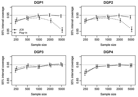
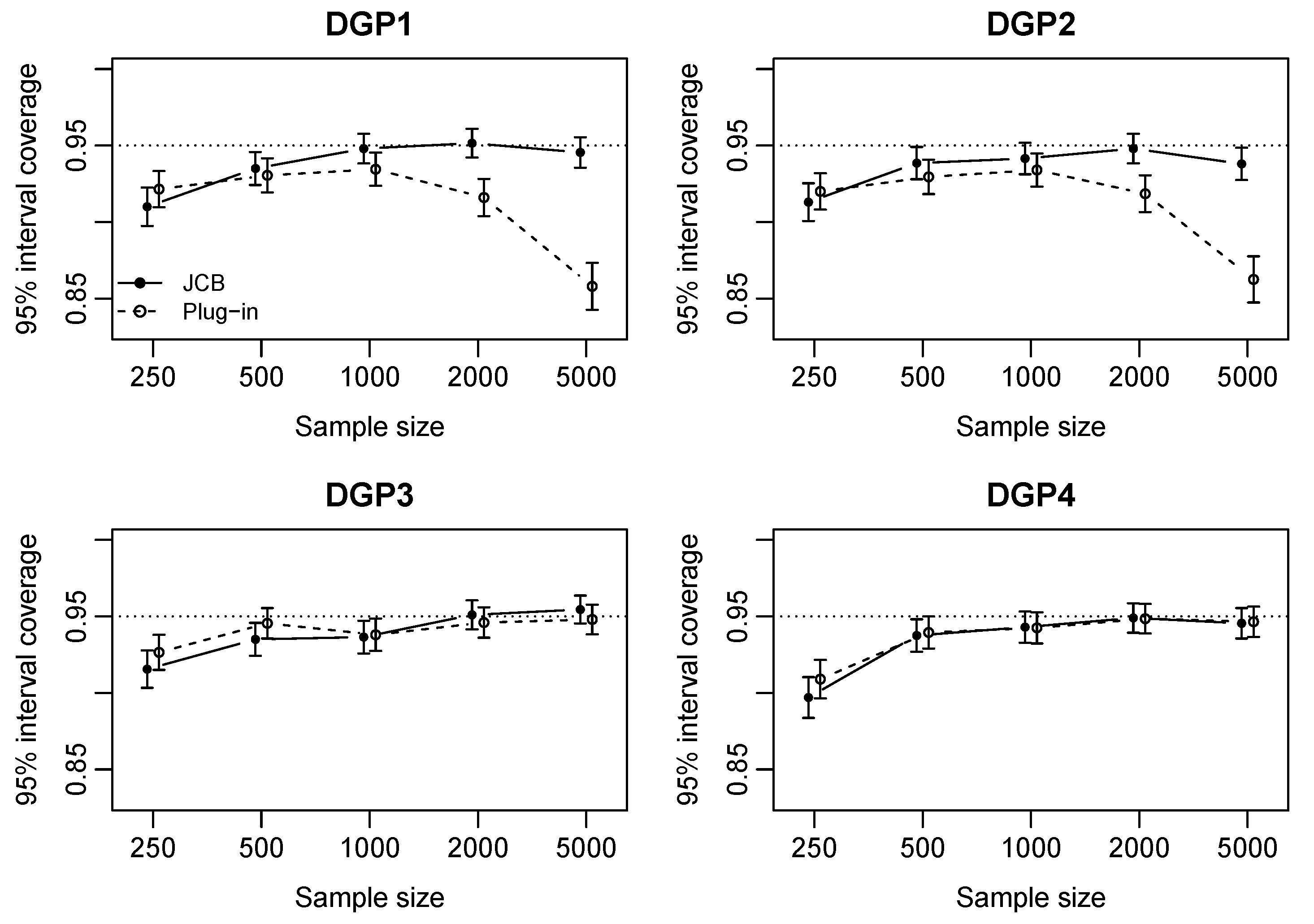
The results of the four baseline designs are summarized in Table 2 at $n=5000$ and, across sample sizes, in Figure 1. Bias is the average deviation of the replicated estimates from the true ATT; SD is the empirical standard deviation of the replicated estimates and SE is the average of their estimated standard errors; RMSE is the root mean squared error; and coverage is the proportion of nominal 95% Wald intervals containing the true ATT. Parentheses give Monte Carlo standard errors (MCSEs), computed as in Table 6 of Morris et al. (2019): $\mathrm{SD}/\sqrt{m}$ for the bias and ${\{\widehat{c}(1-\widehat{c})/m\}}^{1/2}$ for the coverage $\widehat{c}$, where m is the number of successful fits in the cell, equal to 2000 throughout Table 2.

Table 2. Baseline results.

Design	Estimator	Bias (MCSE)	SD	SE	RMSE	Cover. (MCSE)
DGP1	Naive	−0.3485 (0.0017)	0.076	0.076	0.357	0.0035 (0.0013)
DGP1	Plug-in	0.0751 (0.0019)	0.086	0.086	0.114	0.8580 (0.0078)
DGP1	JCB	−0.0041 (0.0018)	0.081	0.080	0.081	0.9455 (0.0051)
DGP2	Naive	−0.3867 (0.0016)	0.070	0.068	0.393	0.0000 (0.0000)
DGP2	Plug-in	0.0542 (0.0015)	0.069	0.067	0.088	0.8625 (0.0077)
DGP2	JCB	0.0016 (0.0015)	0.067	0.065	0.067	0.9380 (0.0054)
DGP3	Naive	−0.3775 (0.0017)	0.075	0.076	0.385	0.0005 (0.0005)
DGP3	Plug-in	0.0243 (0.0017)	0.078	0.080	0.082	0.9480 (0.0050)
DGP3	JCB	−0.0026 (0.0017)	0.074	0.076	0.074	0.9545 (0.0047)
DGP4	Naive	−0.4216 (0.0015)	0.066	0.067	0.427	0.0000 (0.0000)
DGP4	Plug-in	−0.0021 (0.0014)	0.061	0.060	0.061	0.9465 (0.0050)
DGP4	JCB	−0.0021 (0.0014)	0.061	0.060	0.061	0.9455 (0.0051)

Notes: Each cell uses 2000 attempted datasets. Parentheses give Monte Carlo standard errors (MCSEs) of bias and coverage. SD is the Monte Carlo standard deviation; SE is the mean estimated standard error. Intervals are normal 95% Wald intervals.

Figure 1. Coverage against sample size in DGP1–DGP4. Bars are $\pm 1.96$ Monte Carlo standard errors; the horizontal dotted line marks 0.95. Filled circles and solid lines denote JCB; open circles and dashed lines denote the plug-in estimator.

At $n=5000$, JCB has absolute bias below 0.005 in each baseline design, whereas the plug-in biases in DGP1–DGP3 are 0.075, 0.054, and 0.024. Measured against the Monte Carlo standard errors in Table 2, these plug-in departures are 39, 35, and 14 MCSEs from zero, and the associated coverages of 0.8580 in DGP1 and 0.8625 in DGP2 lie about twelve MCSEs below nominal, so they reflect misspecification rather than simulation noise. The JCB departures are smaller by an order of magnitude: only DGP1 exceeds two MCSEs, at $-0.0041$ against an MCSE of 0.0018, and JCB coverage is within 2.3 MCSEs of $0.95$ in every design. In DGP4, where both outcome models are correct, JCB and the plug-in estimator have essentially identical RMSE (0.061); their biases agree to four decimals and both lie 1.5 MCSEs from zero, so this design does not separate them. These comparisons illustrate correctness of the composite working models as a distinct source of robustness, rather than a general advantage over factorized models. The results above are all at $n=5000$, whereas Theorems 2 and 3 are asymptotic and the samples available in applied DID studies are often far smaller. We therefore turn to the behavior of the estimator and of its inference as n falls.

Figure 1 plots coverage against sample size for both estimators in the four baseline designs, with bars of $\pm 1.96$ Monte Carlo standard errors. Two features stand out. First, at $n=250$ neither estimator attains nominal coverage: JCB ranges from 0.897 to 0.916, and its mean estimated standard error is only 0.87 to 0.90 times the Monte Carlo standard deviation, so the asymptotic approximation understates the sampling variability. The gap closes as n grows; by $n=5000$, JCB coverage ranges from 0.938 to 0.955 and that ratio lies between 0.97 and 1.03. Second, the two estimators diverge in DGP1 and DGP2: the plug-in curve peaks near 0.934 at $n=1000$ and then falls to 0.858 and 0.863 at $n=5000$, while JCB stays close to nominal. The plug-in bias settles near 0.07 and 0.05 from $n=500$ onwards, while its standard error shrinks at the rate $n^{-1/2}$, so the ratio of the two grows and the intervals miss increasingly often; this is the finite-sample signature of an inconsistent estimator. In DGP3 and DGP4 the two curves stay close, the smaller plug-in bias in DGP3 not yet being visible in coverage at these sample sizes. Detailed results are reported in Table A2 of Appendix B. We also examine the behavior of the JCB estimator when respondents are scarce, a setting in which its calibration can fail outright; that experiment is reported in Appendix B.1 and Table A4.

6.2. Efficiency Comparison

To illustrate the non-monotonic efficiency ranking discussed in Remark 1, we consider DGP5. Let $e^{*}=p=0.4$ and $r_1^{*}=r_0^{*}=r=0.6$. Define $\mu \left(X\right)=0.5Z_1+0.5Z_2$ and generate $Y_0=\mu \left(X\right)+{\epsilon }_0$, $Y_1=\mu \left(X\right)+g\left(X\right)+2D+{\epsilon }_1$, where $({\epsilon }_0,{\epsilon }_1)$ is mean-zero bivariate normal with unit marginal variances and correlation $\rho \in \{0.2,0.8\}$, independent of $(X,D,R)$. We retain $Y_1$ for every unit and reveal $Y_0$ only when $R=1$. Both MAR restrictions in Remark 1 hold, the ATT is 2, and all probability, density-ratio, and outcome working models on $b^{\left(3\right)}={(1,Z_1,Z_2)}^{\top }$ are correctly specified. The sample sizes are 500, 1000, and 5000.

We directly implement the estimator under Assumption 2.3 of Testa et al. (2026), using low-dimensional logistic and linear regressions. This is a parametric implementation of their estimating equation, not a replication of their random-forest procedure. Write ${\mu }_d^{*}\left(X\right)=\mathbb{E}(Y_0\mid D=d,X)$, ${\nu }_0^{*}\left(X\right)=\mathbb{E}(Y_1\mid D=0,X)$ and $m_0^{*}={\nu }_0^{*}-{\mu }_0^{*}$. The estimator is

$${\widehat{\tau }}_T={\displaystyle \frac{1}{n_1}}{\displaystyle \sum _{i=1}^n}\left[D_i\{{\widehat{U}}_{1i}-{\widehat{m}}_0\left(X_i\right)\}-(1-D_i){\displaystyle \frac{\widehat{e}\left(X_i\right)}{1-\widehat{e}\left(X_i\right)}}\{{\widehat{U}}_{0i}-{\widehat{m}}_0\left(X_i\right)\}\right],$$

(26)

where ${\widehat{m}}_0\left(X\right)={\widehat{\nu }}_0\left(X\right)-{\widehat{\mu }}_0\left(X\right)$, $n_1={\sum }_{i=1}^n{D}_i$ is the number of treated units and ${\widehat{U}}_{di}=Y_{1i}-{\widehat{\mu }}_d\left(X_i\right)-{\displaystyle \frac{R_i}{{\widehat{r}}_d\left(X_i\right)}}\{Y_{0i}-{\widehat{\mu }}_d\left(X_i\right)\}$. Write $V_J=V_{\mathrm{eff}}$ for the semiparametric efficiency bound of the coarsened model in Proposition 1 and $V_T=V_{\mathrm{eff}}^T$ for the bound of the outcome-level model in Remark 1, both evaluated at the generating distribution; the same notation is used for the other designs in Appendix B. In the present design, Proposition 1 and the comparison identity (9) give

$$V_J=2(1-\rho )\left\{{\displaystyle \frac{1}{pr}}+{\displaystyle \frac{1}{(1-p)r}}\right\},V_T=\left(1+{\displaystyle \frac{1}{r}}-2\rho \right)\left\{{\displaystyle \frac{1}{p}}+{\displaystyle \frac{1}{1-p}}\right\}.$$

For $\rho =0.2$, $(V_J,V_T)=(11.1111,9.4444)$; for $\rho =0.8$, they are $(2.7778,4.4444)$. Since $e^{*}$ and $r_d^{*}$ are constant here and $m_1^{*}-m_0^{*}=\tau$, both bounds reduce to functions of $\rho$ alone, and because ${\sigma }_{0,d}^{*2}={\sigma }_{1,d}^{*2}$, Remark 1 places the crossing point at $\rho =1/2$: the two values chosen are symmetric about it, so the ranking reverses, with $V_J>V_T$ at $\rho =0.2$ and $V_J<V_T$ at $\rho =0.8$.

Table 3 confirms this prediction in the simulated data. Both estimators are essentially unbiased, and $\overline{\widehat{V}}$ matches the corresponding bound. The reversal is therefore visible in the estimated variances and not only in the efficiency bounds: $\overline{\widehat{V}}=11.1267$ for JCB against ${\overline{\widehat{V}}}_T=9.4559$ for Testa at $\rho =0.2$, and $2.7765$ against $4.4475$ at $\rho =0.8$. Because all four working models are correctly specified in DGP5, this finding also directly verifies Theorem 1.

Table 3. Efficiency comparison under intersection MAR.

$\mathit{\rho }$	Estimator	Bias (MCSE)	SD	SE	V	$\overline{\widehat{\mathit{V}}}$	Cover. (MCSE)
0.2	JCB	−0.0012 (0.0011)	0.0471	0.0472	11.1111	11.1267	0.9470 (0.0050)
0.2	Testa	−0.0002 (0.0010)	0.0440	0.0435	9.4444	9.4559	0.9405 (0.0053)
0.8	JCB	0.0007 (0.0005)	0.0236	0.0236	2.7778	2.7765	0.9510 (0.0048)
0.8	Testa	0.0004 (0.0007)	0.0296	0.0298	4.4444	4.4475	0.9580 (0.0045)

Notes: V is the semiparametric efficiency bound of the model the estimator is built for, $V_J$ for JCB and $V_T$ for Testa, and $\overline{\widehat{V}}$ is the Monte Carlo average of $n{\widehat{\mathrm{SE}}}^2$. The reported rows use $n=5000$ and 2000 attempted datasets per cell. All other columns are defined as in Table 2. Both estimators are evaluated on the same simulated datasets.

6.3. Correct Factorized Models and Dictionary Sensitivity

Designs DGP6-N and DGP6-L reverse the roles of the two implementations: the probability models are genuinely logistic, so the factorized plug-in estimator is correctly specified, and we can quantify what JCB gives up in that case. They use

$$\begin{array}{cc}\hfill logit{e}^{*}& =-1+1.5Z_1+0.3Z_2,\hfill \\ \hfill logit{r}_1^{*}& =0.3-0.7Z_1+0.2Z_2,\hfill \\ \hfill logit{r}_0^{*}& =-0.2+0.6Z_1-0.2Z_2.\hfill \end{array}$$

These models belong to the factorized working families on $b^{\left(3\right)}$, whereas the composite density ratios generally do not belong to the exponential working family. DGP6-N uses $m_0^{*}=g-4Q$ and $m_1^{*}=g+2+2.5Q$, so both linear outcome models are misspecified. Numerical integration gives $\mathbb{E}(Q\mid D=1)=0.0242$ and $\tau =2.1572$. DGP6-L uses $m_0^{*}=g$, $m_1^{*}=g+2$ and $\tau =2$. Both designs use $n\in \{500,1000\}$ and unit-variance normal outcome-evolution noise.

Design DGP7 turns to the choice of dictionary. It retains the two correct composite ratios and two nonlinear outcome models from DGP1, but changes treatment assignment to

$$logit{e}^{*}=-0.5+0.8(Z_2^2-1/3)+0.6Q.$$

Now, $\mathbb{E}(Q\mid D=1)=0.0329$ and $\tau =2+6.5\mathbb{E}(Q\mid D=1)=2.2137$; the omitted term therefore contributes to the ATT. We use $n\in \{500,1000\}$ and compare JCB with $b^{\left(2\right)}={(1,Z_1)}^{\top }$, $b^{\left(3\right)}$, and $b^{\left(4\right)}={(1,Z_1,Z_2,Q)}^{\top }$ on the same data. The control-group robustness condition fails for $b^{\left(2\right)}$, both density ratios are correct for $b^{\left(3\right)}$, and all four JCB working models are correct for $b^{\left(4\right)}$. The results of DGP6-N, DGP6-L, and DGP7 are summarized in Table 4.

Table 4. Factorized correctness and dictionary sensitivity at $n=1000$.

Design	Estimator	Bias (MCSE)	SD	SE	RMSE	Cover. (MCSE)
DGP6-N	Plug-in	−0.0014 (0.0036)	0.159	0.155	0.159	0.9425 (0.0052)
DGP6-N	JCB	−0.0249 (0.0034)	0.151	0.147	0.153	0.9350 (0.0055)
DGP6-L	Plug-in	0.0022 (0.0024)	0.109	0.107	0.109	0.9445 (0.0051)
DGP6-L	JCB	0.0023 (0.0024)	0.109	0.107	0.109	0.9425 (0.0052)
DGP7	JCB, $K=2$	−0.0337 (0.0048)	0.214	0.206	0.217	0.9390 (0.0054)
DGP7	JCB	−0.0106 (0.0046)	0.207	0.198	0.207	0.9415 (0.0052)
DGP7	JCB, $K=4$	−0.0022 (0.0040)	0.181	0.169	0.181	0.9315 (0.0056)

Notes: Each cell uses 2000 attempted datasets. Parentheses give Monte Carlo standard errors (MCSEs) of bias and coverage. SD is the Monte Carlo standard deviation; SE is the mean estimated standard error. Intervals are normal 95% Wald intervals. Unqualified estimators use $K=3$. The plug-in estimator is shown only for DGP6, where the factorized models are correct; its DGP7 results are in Table A2. True ATTs: DGP6-N = 2.1572; DGP6-L = 2.0000; DGP7 = 2.2137.

At $n=1000$ in DGP6-N, JCB bias is $-0.0249$ (MCSE: 0.0034), compared with $-0.0014$ (MCSE: 0.0036) for the plug-in estimator. JCB is outside its componentwise union model here. Its somewhat smaller RMSE, 0.153 versus 0.159, reflects a finite-sample variance trade-off and does not establish consistency. In DGP6-L both outcome models are correct, and the two estimators have almost identical bias and RMSE.

At $n=1000$, enriching $b^{\left(3\right)}$ to $b^{\left(4\right)}$ reduces JCB bias from $-0.0106$ to $-0.0022$ and RMSE from 0.207 to 0.181; it does not improve coverage (0.9415 versus 0.9315). The $K=4$ calibration fails once in 2000 attempts at $n=500$. Dictionary enrichment can reduce approximation error and variance while making calibration more demanding; its effect on finite-sample coverage is not monotone.

7. Conclusions

This paper studies the estimation of the ATT in a DID design when the outcome evolution is missing at random. We derive the efficient influence function for the coarsened observed-data model and propose a joint covariate balancing estimator that combines treatment and response into a single indicator and calibrates the two group-based density ratios directly, thereby dispensing with the separate estimation of the treatment and response probabilities. The estimator requires only two working models for point estimation, is automatically self-normalized, and attains the semiparametric efficiency bound when all working models are correctly specified. Beyond local efficiency, it is componentwise doubly robust: for each respondent group, correct specification of either the density-ratio model or the outcome-evolution model suffices for consistency, and the weighted least-squares projection makes the same influence-function-based variance estimator valid throughout the union model, so that the resulting inference is doubly robust. The simulation results support the componentwise robustness of the proposed estimator and confirm the efficiency result when all nuisance models are correctly specified, while also highlighting substantial small-sample limitations under low response probabilities. Designs with correctly specified factorized probability models further show that the JCB estimator does not enjoy a universal advantage under model misspecification.

Several extensions merit further study. First, the two-period design studied here is the building block of the group-time average treatment effects of Callaway and Sant’Anna (2021), surveyed together with the recent DID literature in Roth et al. (2023); the joint balancing approach could be extended to multiple periods and staggered adoption, where group-time ATTs would require a family of calibration conditions. Second, the fixed dictionary $b\left(X\right)$ could be allowed to grow with the sample size, connecting the joint balancing approach to sieve-based automatic estimation of the density ratios. Third, relaxing the MAR restriction on the outcome evolution toward instrument- or shadow-variable-based identification under missingness not at random is a natural next step.

Appendix A.1. Proof of the Identification Result (4)

Proof. 

Applying the second identity in (A1) with $g={\omega }_d^{*}$ and using $a_d^{*}{\omega }_d^{*}=e^{*}$ from (5),

$${\displaystyle \frac{1}{p}}\mathbb{E}\left[\{S_1{\omega }_1^{*}\left(X\right)-S_0{\omega }_0^{*}\left(X\right)\}\Delta Y\right]={\displaystyle \frac{1}{p}}\mathbb{E}\left[e^{*}\left(X\right)m_1^{*}\left(X\right)\right]-{\displaystyle \frac{1}{p}}\mathbb{E}\left[e^{*}\left(X\right)m_0^{*}\left(X\right)\right].$$

By Assumption 1(i), $m_1^{*}\left(X\right)=\mathbb{E}[Y_1\left(1\right)-Y_0\left(0\right)\mid D=1,X]$, and by conditional parallel trends (Assumption 1(ii)), $m_0^{*}\left(X\right)=\mathbb{E}[Y_1\left(0\right)-Y_0\left(0\right)\mid D=0,X]=\mathbb{E}[Y_1\left(0\right)-Y_0\left(0\right)\mid D=1,X]$ on the treated support. Hence, the display equals $\mathbb{E}[\mathbb{E}[Y_1\left(1\right)-Y_1\left(0\right)\mid D=1,X]\mid D=1]=\tau$. □

Appendix A.2. Proof of Proposition 1

Proof. 

The proof follows the structure of Hahn (1998) and Sant’Anna and Zhao (2020). The observed-data density with respect to a dominating measure factorizes as

$$f\left(O\right)=f_X\left(x\right)e^{*}{\left(x\right)}^D{\{1-e^{*}\left(x\right)\}}^{1-D}{r}_D^{*}{\left(x\right)}^R{\{1-r_D^{*}\left(x\right)\}}^{1-R}{f}_1{(\Delta y\mid x)}^{DR}{f}_0{(\Delta y\mid x)}^{(1-D)R},$$

where $r_D^{*}\left(x\right)=D{r}_1^{*}\left(x\right)+(1-D)r_0^{*}\left(x\right)$ and $f_d(\Delta y\mid x)$ denotes the conditional density of $\Delta Y$ given $(D=d,R=1,X=x)$; by Assumption 2(i), $m_d^{*}\left(x\right)=\int \Delta y{f}_d(\Delta y\mid x)d\Delta y$. For a regular parametric submodel through the truth, the score takes the form

$$\begin{array}{cc}\hfill S\left(O\right)=& u\left(X\right)\{D-e^{*}\left(X\right)\}+v(D,X)\{R-r_D^{*}\left(X\right)\}\hfill \\ & +DR{s}_1(\Delta Y\mid X)+(1-D)R{s}_0(\Delta Y\mid X)+t\left(X\right),\hfill \end{array}$$

with $\int s_d(\Delta y\mid x)f_d(\Delta y\mid x)d\Delta y=0$ for all x and $\mathbb{E}\left[t\right(X\left)\right]=0$.

We justify the claim that these elements generate the tangent space. The five factors $f_X$, $e^{*}$, $r_D^{*}$, $f_1$, and $f_0$ in the displayed factorization are variation-independent, and the observed-data model places no restriction on any of them: Assumption 2(i) is a restriction on the joint law of $(R,\Delta Y)$ given $(D,X)$, which is not identified from O because $\Delta Y$ is recorded only when $R=1$; it therefore restricts the full-data law but leaves the model for O nonparametric. Consequently, the tangent space is the orthogonal direct sum

$$\mathcal{T}={\mathcal{T}}_X\oplus {\mathcal{T}}_D\oplus {\mathcal{T}}_R\oplus {\mathcal{T}}_1\oplus {\mathcal{T}}_0,$$

where ${\mathcal{T}}_X=\{t\left(X\right):\mathbb{E}t=0,\mathbb{E}{t}^2<\infty \}$, ${\mathcal{T}}_D=\left\{u\left(X\right)\{D-e^{*}\left(X\right)\}\right\}$, ${\mathcal{T}}_R=\left\{v(D,X)\{R-r_D^{*}\left(X\right)\}\right\}$, and ${\mathcal{T}}_d=\{S_d{s}_d(\Delta Y\mid X):\mathbb{E}[s_d\mid D=d,R=1,X]=0\}$, each intersected with $L_2$. Orthogonality of the five summands follows from iterated expectations, using $\mathbb{E}[D-e^{*}\mid X]=0$, $\mathbb{E}[R-r_D^{*}\mid D,X]=0$, and $\mathbb{E}[s_d\mid D=d,R=1,X]=0$. That each summand is generated by regular parametric submodels is standard: for a bounded h in the relevant subspace, the one-dimensional submodel obtained by tilting the corresponding factor by $1+\theta h$ is regular with score h at $\theta =0$, and bounded functions are dense in each summand, so the mean-square closure of the scores is the whole summand. This is precisely the coarsened data construction of Tsiatis (2006, Chapters 7–10), specialized to a two-stage coarsening by D and R; see also Hahn (1998) for the complete-data case. Because the observed-data model is nonparametric, $\mathcal{T}$ is the entire space of mean-zero square-integrable functions of O, so an influence function for $\tau$ is unique and is automatically efficient once it is shown to be an influence function; the verification below therefore establishes both claims at once. Along the submodel, (4) gives

$$\tau \left(\theta \right)={\displaystyle \frac{\int e_{\theta }\left(x\right)\{m_{1,\theta }\left(x\right)-m_{0,\theta }\left(x\right)\}{f}_{X,\theta }\left(x\right)dx}{\int e_{\theta }\left(x\right)f_{X,\theta }\left(x\right)dx}},m_{d,\theta }\left(x\right)=\int \Delta y{f}_{d,\theta }(\Delta y\mid x)d\Delta y,$$

whose pathwise derivative at the truth is

$$\begin{array}{cc}\hfill {\partial }_{\theta }\tau ={\displaystyle \frac{1}{p}}[& \mathbb{E}\left[e^{*}\left(X\right)\int \Delta y{s}_1(\Delta y\mid X)f_1(\Delta y\mid X)d\Delta y\right]\hfill \\ \hfill & -\mathbb{E}\left[e^{*}\left(X\right)\int \Delta y{s}_0(\Delta y\mid X)f_0(\Delta y\mid X)d\Delta y\right]\hfill \\ \hfill & +\mathbb{E}\left[\{m_1^{*}\left(X\right)-m_0^{*}\left(X\right)-\tau \}{\partial }_{\theta }e\left(X\right)\right]\hfill \\ \hfill & +\mathbb{E}\left[\{m_1^{*}\left(X\right)-m_0^{*}\left(X\right)-\tau \}{e}^{*}\left(X\right)t\left(X\right)\right]],\hfill \end{array}$$

(A2)

where ${\partial }_{\theta }e\left(X\right)=\partial e_{\theta }\left(X\right)/\partial \theta {|}_{\theta ={\theta }^{*}}$ denotes the pathwise derivative of the treatment probability along the submodel; matching the Bernoulli score component $u\left(X\right)\{D-e^{*}\left(X\right)\}$ gives ${\partial }_{\theta }e\left(X\right)=u\left(X\right)e^{*}\left(X\right)\{1-e^{*}\left(X\right)\}$. Decompose

$${\phi }_{\mathrm{eff}}\left(O\right)=\overline{u}\left(X\right)\{D-e^{*}\left(X\right)\}+DR{\overline{s}}_1(\Delta Y\mid X)+(1-D)R{\overline{s}}_0(\Delta Y\mid X)+\overline{t}\left(X\right),$$

with $\overline{u}=\{m_1^{*}-m_0^{*}-\tau \}/p$, ${\overline{s}}_1={\omega }_1^{*}\left(X\right)\{\Delta Y-m_1^{*}\left(X\right)\}/p$, ${\overline{s}}_0=-{\omega }_0^{*}\left(X\right)\{\Delta Y-m_0^{*}\left(X\right)\}/p$, and $\overline{t}=e^{*}\left(X\right)\{m_1^{*}-m_0^{*}-\tau \}/p$. Each ${\overline{s}}_d$ integrates to zero against $f_d$, and $\mathbb{E}\left[\overline{t}\left(X\right)\right]=0$ because $p\tau =\mathbb{E}\left[e^{*}(m_1^{*}-m_0^{*})\right]$; hence, ${\phi }_{\mathrm{eff}}\in \mathcal{T}$, and $\mathbb{E}\left[{\phi }_{\mathrm{eff}}\left(O\right)\right]=0$ follows from the same identities. Pairing ${\phi }_{\mathrm{eff}}$ with each score component via iterated expectations, using $\mathbb{E}[D\{D-e^{*}\left(X\right)\}\mid X]=e^{*}\left(X\right)\{1-e^{*}\left(X\right)\}$, $\mathbb{E}[R-r_D^{*}\left(X\right)\mid D,X]=0$, $r_1^{*}{\omega }_1^{*}=1$, $(1-e^{*})r_0^{*}{\omega }_0^{*}=e^{*}$, and the zero conditional means of the residuals $\Delta Y-m_d^{*}\left(X\right)$ given $(D=d,R=1,X)$, all cross-terms vanish and

$$\mathbb{E}\left[{\phi }_{\mathrm{eff}}\left(O\right)S\left(O\right)\right]={\partial }_{\theta }\tau$$

for every regular submodel, with the four surviving pairings matching the four terms of (A2). Therefore, ${\phi }_{\mathrm{eff}}$ is an influence function for $\tau$; being an element of $\mathcal{T}$, it is the efficient influence function, and $V_{\mathrm{eff}}=\mathbb{E}\left[{\phi }_{\mathrm{eff}}^2\right]$ is the semiparametric efficiency bound. □

Appendix A.3. Proof of the Efficiency Comparison in Remark 1

Proof. 

Throughout this subsection we specialize to the design of Testa et al. (2026) under their Assumption 2.3: the post-treatment outcome $Y_1$ is always observed, R indicates that the baseline outcome $Y_0$ is observed, and the observed data are $O^T=(X,D,Y_1,R,R{Y}_0)$, of which $O=(X,D,R,R\Delta Y)$ is a coarsening. We impose the intersection condition (7), that is, $(Y_0,Y_1)\perp \perp R\mid (D,X)$, under which both MAR conditions are satisfied. The two bounds are defined in their respective observed-data models: $V_{\mathrm{eff}}$ in the nonparametric model for O under Assumption 2(i), and $V_{\mathrm{eff}}^T$ in the nonparametric model for $O^T$ under their Assumption 2.3. Write ${\nu }_d^{*}\left(X\right)=\mathbb{E}(Y_1\mid D=d,X)$, ${\mu }_d^{*}\left(X\right)=\mathbb{E}(Y_0\mid D=d,X)$, so that $m_d^{*}={\nu }_d^{*}-{\mu }_d^{*}$, and set

$$\begin{array}{c}\hfill {\sigma }_{1,d}^{*2}\left(X\right)=Var(Y_1\mid D=d,X),{\sigma }_{0,d}^{*2}\left(X\right)=Var(Y_0\mid D=d,X),{\sigma }_{\Delta ,d}^{*2}\left(X\right)=Var(\Delta Y\mid D=d,X).\end{array}$$

Step 1 (Comparison of the two efficient influence functions). Based on Equation (5) in Proposition 2.8 of Testa et al. (2026), the efficient influence function for $\tau$ in the nonparametric model for $O^T$ is given by

$$\begin{array}{cc}\hfill {\phi }_T={\displaystyle \frac{1}{p}}[& D\left\{(Y_1-{\nu }_1^{*})-{\displaystyle \frac{R}{r_1^{*}}}(Y_0-{\mu }_1^{*})\right\}\hfill \\ & -{\displaystyle \frac{(1-D)e^{*}}{1-e^{*}}}\left\{(Y_1-{\nu }_0^{*})-{\displaystyle \frac{R}{r_0^{*}}}(Y_0-{\mu }_0^{*})\right\}+D\{m_1^{*}-m_0^{*}-\tau \}],\hfill \end{array}$$

where the dependence on X is suppressed for notational simplicity. Substituting $\Delta Y-m_d^{*}=(Y_1-{\nu }_d^{*})-(Y_0-{\mu }_d^{*})$ into (6), we obtain ${\phi }_T-{\phi }_{\mathrm{eff}}=\Delta (O,Y_1)$, where $\Delta$ is defined in (8). Under (7), an application of the law of iterated expectations yields $\mathbb{E}[\Delta (O,Y_1)]=0$.

Step 2 (Second and cross-moments). Because $r_d^{*}\left(X\right)=\mathbb{P}(R=1\mid D=d,X)$ and $R^2=R$, for $d\in \{0,1\}$,

$$\mathbb{E}\left[1-{\displaystyle \frac{R}{r_d^{*}}}|D=d,X\right]=0,\mathbb{E}\left[{\left(1-{\displaystyle \frac{R}{r_d^{*}}}\right)}^2|D=d,X\right]={\displaystyle \frac{1-r_d^{*}}{r_d^{*}}},$$

$$\mathbb{E}\left[{\displaystyle \frac{R}{r_d^{*}}}\left(1-{\displaystyle \frac{R}{r_d^{*}}}\right)|D=d,X\right]=-{\displaystyle \frac{1-r_d^{*}}{r_d^{*}}},$$

and, by (7), each of them factorizes from any function of $(Y_0,Y_1)$ given $(D,X)$. The two terms of $\Delta$ are supported on $D=1$ and $D=0$, respectively, so their cross-product vanishes because $D(1-D)=0$. Applying the law of iterated expectations conditional on $(D,X)$ together with the second identity above, the second moment of $\Delta$ is

$$\begin{array}{c}\hfill p^2\mathbb{E}\left({\Delta }^2\right)=\mathbb{E}\left[e^{*}{\displaystyle \frac{1-r_1^{*}}{r_1^{*}}}{\sigma }_{1,1}^{*2}\right]+\mathbb{E}\left[(1-e^{*}){\left({\displaystyle \frac{e^{*}}{1-e^{*}}}\right)}^2{\displaystyle \frac{1-r_0^{*}}{r_0^{*}}}{\sigma }_{1,0}^{*2}\right]={\displaystyle \sum _{d=0}^1}\mathbb{E}\left[q_d^{*}{\sigma }_{1,d}^{*2}\right],\end{array}$$

where $\mathbb{E}[{(Y_1-{\nu }_d^{*})}^2\mid D=d,X]={\sigma }_{1,d}^{*2}$, $q_1^{*}={\displaystyle \frac{e^{*}\{1-r_1^{*}\}}{r_1^{*}}}$, and $q_0^{*}={\displaystyle \frac{{\left(e^{*}\right)}^2\{1-r_0^{*}\}}{\{1-e^{*}\}{r}_0^{*}}}$. By a similar argument, the cross-moment of ${\phi }_{\mathrm{eff}}$ and $\Delta$ can be evaluated component by component. The component $D\{m_1^{*}-m_0^{*}-\tau \}$ of ${\phi }_{\mathrm{eff}}$ is a function of $(D,X)$; it is orthogonal to the first term of $\Delta$ by the first identity above, and to the second term because $D(1-D)=0$. For the remaining components, $S_1{\omega }_1^{*}=DR/r_1^{*}$ and $S_0{\omega }_0^{*}=(1-D)R{e}^{*}/\left\{(1-e^{*})r_0^{*}\right\}$, so the third identity gives

$$\begin{array}{c}\hfill p^2\mathbb{E}({\phi }_{\mathrm{eff}}\Delta )=-\mathbb{E}\left[e^{*}{\displaystyle \frac{1-r_1^{*}}{r_1^{*}}}{c}_1^{*}\right]-\mathbb{E}\left[{\displaystyle \frac{{\left(e^{*}\right)}^2}{1-e^{*}}}{\displaystyle \frac{1-r_0^{*}}{r_0^{*}}}{c}_0^{*}\right]=-{\displaystyle \sum _{d=0}^1}\mathbb{E}\left[q_d^{*}{c}_d^{*}\right],\end{array}$$

where $c_d^{*}=Cov(\Delta Y,Y_1\mid D=d,X)$.

Step 3 (Conclusion). Since ${\phi }_T={\phi }_{\mathrm{eff}}+\Delta$ and both terms have mean zero, $V_{\mathrm{eff}}^T=\mathbb{E}\left({\phi }_T^2\right)=V_{\mathrm{eff}}+2\mathbb{E}({\phi }_{\mathrm{eff}}\Delta )+\mathbb{E}\left({\Delta }^2\right)$. Combining the two displays in Step 2,

$$p^2\left(V_{\mathrm{eff}}^T-V_{\mathrm{eff}}\right)=p^2\left\{2\mathbb{E}({\phi }_{\mathrm{eff}}\Delta )+\mathbb{E}\left({\Delta }^2\right)\right\}={\displaystyle \sum _{d=0}^1}\mathbb{E}\left[q_d^{*}\left({\sigma }_{1,d}^{*2}-2c_d^{*}\right)\right].$$

Since $c_d^{*}=Cov(Y_1-Y_0,Y_1\mid D=d,X)={\sigma }_{1,d}^{*2}-Cov(Y_0,Y_1\mid D=d,X)$,

$${\sigma }_{1,d}^{*2}-2c_d^{*}=2Cov(Y_0,Y_1\mid D=d,X)-{\sigma }_{1,d}^{*2}=-\left\{{\sigma }_{\Delta ,d}^{*2}-{\sigma }_{0,d}^{*2}\right\},$$

which is (9). □

Appendix A.4. Proof of Proposition 2

Proof. 

Applying the identities in (A1) to each term of (10),

$$p{\tau }_{\mathrm{dr}}=\mathbb{E}\left[e^{*}(m_1-m_0)\right]+\mathbb{E}\left[a_1^{*}{\omega }_1(m_1^{*}-m_1)\right]-\mathbb{E}\left[a_0^{*}{\omega }_0(m_0^{*}-m_0)\right],$$

where all functions are evaluated at X. Subtracting $p\tau =\mathbb{E}\left[e^{*}(m_1^{*}-m_0^{*})\right]$ and rearranging,

$$p({\tau }_{\mathrm{dr}}-\tau )=\mathbb{E}\left[(a_1^{*}{\omega }_1-e^{*})(m_1^{*}-m_1)\right]-\mathbb{E}\left[(a_0^{*}{\omega }_0-e^{*})(m_0^{*}-m_0)\right].$$

(A3)

Each term in (A3) is the product of a weighting error and an outcome error for one respondent group. If ${\omega }_d={\omega }_d^{*}$, then $a_d^{*}{\omega }_d=e^{*}$ by (5); if $m_d=m_d^{*}$, then $m_d^{*}-m_d=0$. Hence, under the componentwise condition of Proposition 2, both terms vanish and ${\tau }_{\mathrm{dr}}=\tau$. □

Appendix A.5. Auxiliary Lemmas

Lemma A1 (Primitive conditions imply the asymptotic regularity used in Section 5).

Let Assumptions 1–3 hold and let $d\in \{0,1\}$. Then,

 (a) 

The population calibration objective ${\lambda }_d\mapsto \mathbb{E}[S_d{G}_d\left\{b{\left(X\right)}^{\top }{\lambda }_d\right\}-Db{\left(X\right)}^{\top }{\lambda }_d]$, with $G_d^{\prime }=g_d$, is strictly convex on ${\Lambda }_d$, so the interior solution ${\lambda }_d^0$ of Assumption 3(iii) is its global minimizer, and the Jacobian $J_d=\mathbb{E}\left[S_d{\dot{g}}_d\left\{b{\left(X\right)}^{\top }{\lambda }_d^0\right\}b\left(X\right)b{\left(X\right)}^{\top }\right]$ is finite and positive definite;

 (b) 

The population projection equation has the unique solution ${\beta }_d^0$ of (23) , whose design matrix is exactly the calibration Jacobian $J_d$, and the projection is a weighted least-squares fit with weights $S_d{\dot{g}}_d^0\left(X\right)$;

 (c) 

With probability approaching one, the sample problem (12) has a unique minimizer ${\widehat{\lambda }}_d$ in the interior of ${\Lambda }_d$, and ${\widehat{\lambda }}_d\stackrel{p}{\to }{\lambda }_d^0$ and ${\widehat{\beta }}_d\stackrel{p}{\to }{\beta }_d^0$;

 (d) 

$({\widehat{\lambda }}_d,{\widehat{\beta }}_d)$ is root-n consistent and asymptotically linear, with

$$\sqrt{n}({\widehat{\lambda }}_d-{\lambda }_d^0)={\displaystyle \frac{1}{\sqrt{n}}}{\displaystyle \sum _{i=1}^n}{J}_d^{-1}\{D_i-S_{di}{\omega }_d^0\left(X_i\right)\}b\left(X_i\right)+o_p\left(1\right),$$

and

$$\sqrt{n}({\widehat{\beta }}_d-{\beta }_d^0)=J_d^{-1}{\displaystyle \frac{1}{\sqrt{n}}}{\displaystyle \sum _{i=1}^n}\left[{\zeta }_d^0\left(O_i\right)+H_d{J}_d^{-1}\{D_i-S_{di}{\omega }_d^0\left(X_i\right)\}b\left(X_i\right)\right]+o_p\left(1\right),$$

where

$$\begin{array}{cc}\hfill {\zeta }_d^0\left(O\right)& =S_d{\dot{g}}_d^0\left(X\right)b\left(X\right)\{\Delta Y-b{\left(X\right)}^{\top }{\beta }_d^0\},\hfill \\ \hfill H_d& =\mathbb{E}\left[S_d{\ddot{g}}_d\left\{b{\left(X\right)}^{\top }{\lambda }_d^0\right\}b\left(X\right)b{\left(X\right)}^{\top }\{\Delta Y-b{\left(X\right)}^{\top }{\beta }_d^0\}\right];\hfill \end{array}$$

 (e) 

The calibration and projection estimating functions, indexed by $({\lambda }_d,{\beta }_d)$ in a neighborhood of $({\lambda }_d^0,{\beta }_d^0)$, are continuously differentiable in the parameters; the functions and their first derivatives have square-integrable envelopes, and the functions satisfy a parameter-Lipschitz bound with a square-integrable random coefficient.

Lemma A2 (Population calibration and projection identities).

Let Assumptions 1–3 hold. For $d\in \{0,1\}$,

 (a) 

$\mathbb{E}\left[\{a_d^{*}\left(X\right){\omega }_d^0\left(X\right)-e^{*}\left(X\right)\}b\left(X\right)\right]=0$;

 (b) 

If ${\omega }_d^{*}\left(X\right)=g_d\left\{b{\left(X\right)}^{\top }{\overline{\lambda }}_d\right\}$ for some ${\overline{\lambda }}_d\in {\mathbb{R}}^K$, then ${\overline{\lambda }}_d={\lambda }_d^0$, so that ${\mathcal{W}}_d$ holds and $a_d^{*}{\omega }_d^0=e^{*}$ almost surely;

 (c) 

If $m_d^{*}\left(X\right)=b{\left(X\right)}^{\top }{\overline{\beta }}_d$ for some ${\overline{\beta }}_d\in {\mathbb{R}}^K$, then ${\overline{\beta }}_d={\beta }_d^0$, so that ${\mathcal{M}}_d$ holds and ${\ell }_d^0=m_d^{*}$ almost surely.

The two lemmas play different roles. Lemma A1 converts Assumption 3 into the asymptotic regularity that the later proofs use: a strictly convex population calibration objective with a finite, positive-definite Jacobian, a unique population projection coefficient whose design matrix is that same Jacobian, consistency of $({\widehat{\lambda }}_d,{\widehat{\beta }}_d)$, their root-n asymptotic linearity, and square-integrable envelopes for the estimating functions. Parts (c)–(e) are what justify the uniform laws of large numbers, mean-value expansions and central limit theorems invoked in the proofs of Theorems 2 and 3.

Lemma A2 records the population identities behind the double-robustness arguments. Part (a) is the population counterpart of the sample balancing condition (11); it holds at the pseudo-true parameter whether or not the working models are correctly specified, and it is what removes each respondent group’s bias term. Parts (b)–(c) state that if the true density ratio ${\omega }_d^{*}$ or the true outcome evolution $m_d^{*}$ belongs to the corresponding working family, then the pseudo-true parameter recovers it, so that ${\mathcal{W}}_d$ holds at ${\lambda }_d^0$ or ${\mathcal{M}}_d$ holds at ${\beta }_d^0$. The lemma is used in the proofs of Theorems 1–3.

Proof of Lemma A1.

Fix $d\in \{0,1\}$ and let $C_{\Lambda }={\sup }_{{\lambda }_d\in {\Lambda }_d}\parallel {\lambda }_d\parallel <\infty$, which is finite by Assumption 3(iii). By Assumption 3(i), ${|b\left(X\right)}^{\top }{\lambda }_d|\le C_b{C}_{\Lambda }=:C$ almost surely, uniformly in ${\lambda }_d\in {\Lambda }_d$. Because $g_d$ is continuous and strictly positive and ${\dot{g}}_d$ is continuous and strictly positive by Assumption 3(ii), the constants

$$\begin{array}{cc}\hfill 0<c_1& =\underset{\left|u\right|\le C}{\min }{\dot{g}}_d\left(u\right)\le \underset{\left|u\right|\le C}{\max }{\dot{g}}_d\left(u\right)=c_2<\infty ,\hfill \\ \hfill 0<c_3& =\underset{\left|u\right|\le C}{\min }{g}_d\left(u\right)\le \underset{\left|u\right|\le C}{\max }{g}_d\left(u\right)=c_4<\infty ,\hfill \end{array}$$

are well defined, since a continuous positive function attains its bounds on a compact interval. By Assumption 3(ii), $c_5:={\max }_{\left|u\right|\le C}\left|{\ddot{g}}_d\left(u\right)\right|<\infty$. Hence, $g_d$ and ${\dot{g}}_d$ are Lipschitz on $[-C,C]$, with constants $c_2$ and $c_5$, respectively.

(a) The population objective $Q_d\left({\lambda }_d\right)=\mathbb{E}[S_d{G}_d\left\{b{\left(X\right)}^{\top }{\lambda }_d\right\}-Db{\left(X\right)}^{\top }{\lambda }_d]$ is finite on ${\Lambda }_d$ and twice continuously differentiable, with ${\nabla }^2{Q}_d\left({\lambda }_d\right)=\mathbb{E}\left[S_d{\dot{g}}_d\left\{b{\left(X\right)}^{\top }{\lambda }_d\right\}b\left(X\right)b{\left(X\right)}^{\top }\right]⪰c_1\mathbb{E}\left[S_{d}b\left(X\right)b{\left(X\right)}^{\top }\right]\succ 0$ by Assumption 3(i). Hence, $Q_d$ is strictly convex on the convex set ${\Lambda }_d$, and the interior stationary point ${\lambda }_d^0$ of Assumption 3(iii) is its global minimizer. The same display at ${\lambda }_d^0$ shows that $J_d$ is positive definite, and $J_d⪯c_2{C}_b^2{I}_K$ shows that it is finite.

(b) The population projection equation is linear in ${\beta }_d$ with coefficient matrix $\mathbb{E}\left[S_d{\dot{g}}_d^0\left(X\right)b\left(X\right)b{\left(X\right)}^{\top }\right]=J_d$, which by (a) is nonsingular; the unique solution is therefore (23), and it is finite because $\parallel b\parallel \le C_b$, ${\dot{g}}_d^0\le c_2$ and $\mathbb{E}(\Delta Y^2)<\infty$. Since ${\dot{g}}_d^0>0$, the equation is the normal equation of a genuine weighted least-squares fit.

(c) The class $\{S_d{G}_d\left\{b{\left(X\right)}^{\top }{\lambda }_d\right\}-Db{\left(X\right)}^{\top }{\lambda }_d:{\lambda }_d\in {\Lambda }_d\}$ is uniformly bounded by ${\max }_{\left|u\right|\le C}\left|G_d\left(u\right)\right|+C$ and is Lipschitz in ${\lambda }_d$ with constant $(c_4+1)C_b$, hence Glivenko–Cantelli; therefore, ${\sup }_{{\lambda }_d\in {\Lambda }_d}|{\widehat{Q}}_d\left({\lambda }_d\right)-Q_d\left({\lambda }_d\right)|\stackrel{p}{\to }0$, where ${\widehat{Q}}_d$ is the sample objective in (12). Both objectives are convex, and $Q_d$ has a unique minimizer in the interior of ${\Lambda }_d$, so the standard argument for convex M-estimation (Newey & McFadden, 1994) gives ${\widehat{\lambda }}_d\stackrel{p}{\to }{\lambda }_d^0$ and, with probability approaching one, ${\widehat{\lambda }}_d$ lies in the interior of ${\Lambda }_d$ and solves (11). Uniqueness holds with probability approaching one because ${\nabla }^2{\widehat{Q}}_d⪰c_1\widehat{\mathbb{E}}\left[S_{d}b{b}^{\top }\right]$ and $\widehat{\mathbb{E}}\left[S_{d}b{b}^{\top }\right]\stackrel{p}{\to }\mathbb{E}\left[S_{d}b{b}^{\top }\right]\succ 0$. For ${\beta }_d$, ${\widehat{\beta }}_d$ solves a linear system whose matrix $\widehat{\mathbb{E}}\left[S_d{\dot{g}}_d\left\{b{\left(X\right)}^{\top }{\widehat{\lambda }}_d\right\}b{b}^{\top }\right]$ converges in probability to $J_d$ by the same uniform law and the continuity of ${\dot{g}}_d$, and whose right-hand side converges to $\mathbb{E}[S_d{\dot{g}}_d^{0}b\Delta Y]$; hence, ${\widehat{\beta }}_d\stackrel{p}{\to }{\beta }_d^0$.

(d) On the event that ${\widehat{\lambda }}_d$ is an interior solution, the integral form of the mean-value expansion of the sample calibration equation gives

$$0=\widehat{\mathbb{E}}\left[\{S_d{\omega }_d^0\left(X\right)-D\}b\left(X\right)\right]+{\overline{J}}_d({\widehat{\lambda }}_d-{\lambda }_d^0),$$

where

$${\overline{J}}_d={\int }_0^1\widehat{\mathbb{E}}\left[S_d{\dot{g}}_d\left\{b{\left(X\right)}^{\top }[{\lambda }_d^0+t({\widehat{\lambda }}_d-{\lambda }_d^0)]\right\}b\left(X\right)b{\left(X\right)}^{\top }\right]dt.$$

The integrand has a bounded envelope and is Lipschitz in the calibration parameter, with constant $c_5{C}_b^3$. A uniform law of large numbers, consistency from part (c), and continuity therefore give ${\overline{J}}_d\stackrel{p}{\to }{J}_d\succ 0$. Rearranging and applying the central limit theorem to $\{D_i-S_{di}{\omega }_d^0\left(X_i\right)\}b\left(X_i\right)$, which has mean zero and a finite second moment, yields the stated asymptotic expansion for ${\widehat{\lambda }}_d$.

For the projection coefficient, use ${\zeta }_d^0$ and $H_d$ as defined in part (d) of the lemma. The derivatives of the projection equation with respect to ${\lambda }_d^{\top }$ and ${\beta }_d^{\top }$ have population limits $H_d$ and $-J_d$, respectively. They are continuous in the parameters and dominated by an integrable envelope, as shown in part (e). Their uniform laws of large numbers, consistency from part (c), and the integral mean-value expansion therefore give

$$\{J_d+o_p\left(1\right)\}\sqrt{n}({\widehat{\beta }}_d-{\beta }_d^0)={\displaystyle \frac{1}{\sqrt{n}}}{\displaystyle \sum _{i=1}^n}{\zeta }_d^0\left(O_i\right)+\{H_d+o_p\left(1\right)\}\sqrt{n}({\widehat{\lambda }}_d-{\lambda }_d^0).$$

Since $J_d$ is nonsingular, $\sqrt{n}({\widehat{\lambda }}_d-{\lambda }_d^0)=O_p\left(1\right)$, and the sum on the right is $O_p\left(1\right)$, this first establishes $\sqrt{n}({\widehat{\beta }}_d-{\beta }_d^0)=O_p\left(1\right)$ and then yields

$$J_d\sqrt{n}({\widehat{\beta }}_d-{\beta }_d^0)={\displaystyle \frac{1}{\sqrt{n}}}{\displaystyle \sum _{i=1}^n}{\zeta }_d^0\left(O_i\right)+H_d\sqrt{n}({\widehat{\lambda }}_d-{\lambda }_d^0)+o_p\left(1\right).$$

Here, $\mathbb{E}\left[{\zeta }_d^0\left(O\right)\right]=0$ by the population projection equation, and ${\zeta }_d^0$ has a finite second moment. Substituting the expansion for ${\widehat{\lambda }}_d$ gives the stated expansion for ${\widehat{\beta }}_d$. Thus, both nuisance estimators are root-n consistent and asymptotically linear.

(e) Write $b=b\left(X\right)$, $u=b^{\top }{\lambda }_d$, and $r_{\beta }=\Delta Y-b^{\top }{\beta }_d$. The two functions used in Appendices Appendix A.8 and Appendix A.9 are

$$h_d(O;{\lambda }_d,{\beta }_d)=S_d{g}_d\left(u\right)r_{\beta },{\zeta }_d(O;{\lambda }_d,{\beta }_d)=S_d{\dot{g}}_d\left(u\right)b{r}_{\beta },$$

or products of them with D or components of b. Their parameter derivatives are

$$\begin{array}{cccc}\hfill {\nabla }_{{\lambda }_d}{h}_d& =S_d{\dot{g}}_d\left(u\right)b{r}_{\beta },\hfill & \hfill {\nabla }_{{\beta }_d}{h}_d& =-S_d{g}_d\left(u\right)b,\hfill \\ \hfill {\displaystyle \frac{\partial {\zeta }_d}{\partial {\lambda }_d^{\top }}}& =S_d{\ddot{g}}_d\left(u\right)b{b}^{\top }{r}_{\beta },\hfill & \hfill {\displaystyle \frac{\partial {\zeta }_d}{\partial {\beta }_d^{\top }}}& =-S_d{\dot{g}}_d\left(u\right)b{b}^{\top }.\hfill \end{array}$$

These derivatives exist and are continuous by Assumption 3(ii). The calibration estimating function $\{S_d{g}_d\left(u\right)-D\}b$ is also continuously differentiable, with derivative $S_d{\dot{g}}_d\left(u\right)b{b}^{\top }$.

Let $\mathcal{K}$ be a compact convex neighborhood of ${\beta }_d^0$ and $B_{\beta }={\sup }_{{\beta }_d\in \mathcal{K}}\parallel {\beta }_d\parallel$. Since $|r_{\beta }|\le |\Delta Y|+C_b{B}_{\beta }$, the functions above and their first derivatives are bounded in norm, uniformly on ${\Lambda }_d\times \mathcal{K}$, by

$$F_d\left(O\right)=A_d(1+|\Delta Y\left|\right),$$

where $A_d<\infty$ depends only on $C_b$, $C_{\Lambda }$, $c_2$, $c_4$, $c_5$, and $\mathcal{K}$. Products with D or components of b obey a bound of the same form. Integrating the first derivatives along the segment between any two parameter values $\theta ={({\lambda }_d^{\top },{\beta }_d^{\top })}^{\top }$ and $\tilde{\theta }$ gives

$$|h_d(O;\theta )-h_d(O;\tilde{\theta })|+\parallel {\zeta }_d(O;\theta )-{\zeta }_d(O;\tilde{\theta })\parallel \le F_d\left(O\right)\parallel \theta -\tilde{\theta }\parallel ,$$

after increasing $A_d$ if necessary. By Assumption 3(i), $\mathbb{E}\left[F_d{\left(O\right)}^4\right]<\infty$, so this is a square-integrable random Lipschitz coefficient and envelope, and the squared functions have integrable envelopes.

On the compact parameter neighborhood, the estimating functions, their first derivatives, and the squared estimating functions are continuous in the parameters and have integrable envelopes. Hence, uniform laws of large numbers apply. Together with consistency, these justify the convergence of the sample Jacobians in part (d) and the consistency of the variance estimator. At the limiting parameter values, square integrability ensures the ordinary central limit theorems used below. □

Proof of Lemma A2.

(a) Applying the first identity in (A1) coordinatewise, together with $\mathbb{E}\left[Db\left(X\right)\right]=\mathbb{E}\left[e^{*}\left(X\right)b\left(X\right)\right]$, the population calibration equation in Assumption 3(iii) becomes $\mathbb{E}\left[\{a_d^{*}{\omega }_d^0-e^{*}\}b\right]=0$. (b) By (5), $a_d^{*}{\omega }_d^{*}=e^{*}$, so ${\overline{\lambda }}_d$ solves the population calibration equation; uniqueness in Assumption 3(iii) gives ${\overline{\lambda }}_d={\lambda }_d^0$, and ${\mathcal{W}}_d$ holds with $a_d^{*}{\omega }_d^0=a_d^{*}{\omega }_d^{*}=e^{*}$. (c) If $m_d^{*}=b^{\top }{\overline{\beta }}_d$, the second identity in (A1) gives

$$\mathbb{E}\left[S_d{\dot{g}}_d^0\left(X\right)b\left(X\right)\{\Delta Y-b{\left(X\right)}^{\top }{\overline{\beta }}_d\}\right]=\mathbb{E}\left[a_d^{*}\left(X\right){\dot{g}}_d^0\left(X\right)b\left(X\right)\{m_d^{*}\left(X\right)-b{\left(X\right)}^{\top }{\overline{\beta }}_d\}\right]=0,$$

so ${\overline{\beta }}_d$ solves the population projection equation; uniqueness (Lemma A1(b)) gives ${\overline{\beta }}_d={\beta }_d^0$, and ${\mathcal{M}}_d$ holds with ${\ell }_d^0=b{\left(X\right)}^{\top }{\beta }_d^0=m_d^{*}$. □

Appendix A.6. Existence of a Finite Calibration Solution Under the Exponential Link

Here, we discuss the existence of a finite solution to the sample calibration problem in (12) under the exponential link; i.e., $g_d(·)=\exp (·)$, for which $G_d(·)=\exp (·)$. Under this link, (12) is an exponential tilting, or entropy balancing, problem (Graham et al., 2012; Hainmueller, 2012). Recall that the first element of $b\left(X\right)$ is the constant $b_1\equiv 1$, and suppose $\widehat{\mathbb{E}}\left[S_{d}b\left(X\right)b{\left(X\right)}^{\top }\right]$ is nonsingular. Then, the sample objective in (12), minimized over ${\mathbb{R}}^K$, has a minimizer only if the support condition

$${\left({\sum }_{i=1}^n{D}_i\right)}^{-1}{\sum }_{i=1}^n{D}_{i}b\left(X_i\right)\in riconv\left\{b\left(X_i\right):S_{di}=1\right\},$$

(A4)

where ri denotes the relative interior. Equivalently, ${\overline{b}}_T\in riconv{\mathcal{B}}_d$, where ${\overline{b}}_T=n_1^{-1}{\sum }_{i=1}^n{D}_{i}b\left(X_i\right)$, $n_1={\sum }_{i=1}^n{D}_i$, and ${\mathcal{B}}_d=\{b\left(X_i\right):S_{di}=1\}$. The minimizer, when it exists, is unique because the objective is strictly convex.

Two consequences are worth recording. First, the population analogue of (A4) is implied by Assumptions 1(iii) and 2(ii) with the factorization (2), since these guarantee $a_d^{*}\left(X\right)>0$ on the covariate support of the treated, so that the treated distribution of $b\left(X\right)$ is dominated by the group-d respondent distribution; the sample condition then holds with probability approaching one. Second, condition (A4) shows exactly how the risk of failure scales: (A4) is a statement in ${\mathbb{R}}^K$ about ${\sum }_i{S}_{di}$ points, so it becomes more demanding as K increases or as the number of respondents in the smaller group falls, which is the formal counterpart of separation in logistic regression and of the convex-hull condition in empirical likelihood. Condition (A4) therefore fails in exactly the situations practitioners worry about: a comparison group with few respondents; a covariate region populated by treated units but not by group-d respondents; or a dictionary rich enough that the treated mean escapes the K-dimensional hull.

Proof. 

Write $nL\left(\lambda \right)={\sum }_{i:S_{di}=1}\exp \left\{b{\left(X_i\right)}^{\top }\lambda \right\}-n_1{\overline{b}}_T^{\top }\lambda$ for n times the objective in (12). Its Hessian is ${\sum }_{i:S_{di}=1}\exp \left\{b{\left(X_i\right)}^{\top }\lambda \right\}b\left(X_i\right)b{\left(X_i\right)}^{\top }$, which is positive definite because $\widehat{\mathbb{E}}\left[S_{d}b{b}^{\top }\right]$ is nonsingular and the exponential weights are strictly positive; hence, L is strictly convex. At a minimizer ${\widehat{\lambda }}_d$ the first-order condition is ${\sum }_{i:S_{di}=1}\exp \left\{b{\left(X_i\right)}^{\top }{\widehat{\lambda }}_d\right\}b\left(X_i\right)=n_1{\overline{b}}_T$. Its first coordinate, which exists because $b_1\equiv 1$, gives ${\sum }_{i:S_{di}=1}\exp \left\{b{\left(X_i\right)}^{\top }{\widehat{\lambda }}_d\right\}=n_1$. Hence, $p_i=\exp \left\{b{\left(X_i\right)}^{\top }{\widehat{\lambda }}_d\right\}/n_1$ are strictly positive, sum to one, and satisfy ${\sum }_i{p}_{i}b\left(X_i\right)={\overline{b}}_T$, which exhibits ${\overline{b}}_T$ as a convex combination of ${\mathcal{B}}_d$ with all weights strictly positive, that is, ${\overline{b}}_T\in riconv{\mathcal{B}}_d$. □

Appendix A.7. Proof of Theorem 1

Proof. 

If ${\mathcal{W}}_d$ and ${\mathcal{M}}_d$ hold for both $d\in \{0,1\}$, then the union condition (20) also holds. Hence, Equation (25) in Theorem 3 yields

$$\sqrt{n}({\widehat{\tau }}_{\mathrm{JCB}}-\tau )={\displaystyle \frac{1}{\sqrt{n}}}{\displaystyle \sum _{i=1}^n}{\psi }_i^0+o_p\left(1\right)\stackrel{d}{\to }\mathcal{N}(0,V^0),V^0=\mathbb{E}\left[{\left({\psi }_i^0\right)}^2\right].$$

The proof of Equation (25) is provided in Appendix A.9. Obviously, when ${\omega }_d^0={\omega }_d^{*}$ and ${\ell }_d^0=m_d^{*}$ for both d, we have ${\psi }_i^0={\phi }_{\mathrm{eff}}\left(O_i\right)$ in (A10), and hence $V^0=\mathbb{E}\left[{\phi }_{\mathrm{eff}}{\left(O\right)}^2\right]=V_{\mathrm{eff}}$. □

Appendix A.8. Proof of Theorem 2

Proof. 

By Lemma A1(c), ${\widehat{\lambda }}_d\stackrel{p}{\to }{\lambda }_d^0$ and the law of large numbers gives $\widehat{p}\stackrel{p}{\to }p>0$. The envelope conditions supplied by Lemma A1(e) justify a uniform law of large numbers for ${\lambda }_d\mapsto \widehat{\mathbb{E}}[S_d{g}_d\left\{b{\left(X\right)}^{\top }{\lambda }_d\right\}\Delta Y]$ in a neighborhood of ${\lambda }_d^0$, so by the continuous mapping theorem,

$${\widehat{\tau }}_{\mathrm{JCB}}\stackrel{p}{\to }{\displaystyle \frac{1}{p}}\mathbb{E}[\{S_1{\omega }_1^0\left(X\right)-S_0{\omega }_0^0\left(X\right)\}\Delta Y]={\displaystyle \frac{1}{p}}\left[\mathbb{E}\left[a_1^{*}{\omega }_1^0{m}_1^{*}\right]-\mathbb{E}\left[a_0^{*}{\omega }_0^0{m}_0^{*}\right]\right],$$

(A5)

where the equality uses (A1). Combining (4) with (A1) evaluated at ${\omega }_d^{*}$ and using $a_d^{*}{\omega }_d^{*}=e^{*}$ gives $p\tau =\mathbb{E}\left[e^{*}(m_1^{*}-m_0^{*})\right]$. Hence,

$$p\left(plim{\widehat{\tau }}_{\mathrm{JCB}}-\tau \right)=\mathbb{E}\left[(a_1^{*}{\omega }_1^0-e^{*})m_1^{*}\right]-\mathbb{E}\left[(a_0^{*}{\omega }_0^0-e^{*})m_0^{*}\right].$$

(A6)

Because ${\ell }_d^0=b{\left(X\right)}^{\top }{\beta }_d^0$, Lemma A2(a) yields $\mathbb{E}\left[(a_d^{*}{\omega }_d^0-e^{*}){\ell }_d^0\right]=0$; subtracting these zero terms from (A6) gives the product-bias formula (21). Consider component d. Under ${\mathcal{W}}_d$, Lemma A2(b) gives $a_d^{*}{\omega }_d^0-e^{*}=0$ almost surely. Under ${\mathcal{M}}_d$, $m_d^{*}=b^{\top }{\beta }_d^0$ is linear in b, so $\mathbb{E}\left[(a_d^{*}{\omega }_d^0-e^{*})m_d^{*}\right]=0$ by Lemma A2(a). Under the union condition (20), both terms in (A6) therefore vanish, and ${\widehat{\tau }}_{\mathrm{JCB}}\stackrel{p}{\to }\tau$. □

Appendix A.9. Proof of Theorem 3

Proof. 

Let ${\beta }^0={({\beta }_1^{0\top },{\beta }_0^{0\top })}^{\top }$ be defined by (23). The proof proceeds in six steps.

Step 1 (Augmented representation). The sample calibration condition (11) implies $\widehat{\mathbb{E}}\left[S_d{\widehat{\omega }}_d\left(X\right)b{\left(X\right)}^{\top }{\beta }_d\right]=\widehat{\mathbb{E}}\left[Db{\left(X\right)}^{\top }{\beta }_d\right]$ for every ${\beta }_d\in {\mathbb{R}}^K$; adding and subtracting these quantities in (13) yields (14). Evaluating (14) at $\beta ={\beta }^0$ and subtracting $\tau$,

$$\widehat{p}({\widehat{\tau }}_{\mathrm{JCB}}-\tau )=\widehat{\mathbb{E}}\left[D\{b{\left(X\right)}^{\top }({\beta }_1^0-{\beta }_0^0)-\tau \}+{\displaystyle \sum _{d=0}^1}{s}_d{S}_d{g}_d\left\{b{\left(X\right)}^{\top }{\widehat{\lambda }}_d\right\}\{\Delta Y-b{\left(X\right)}^{\top }{\beta }_d^0\}\right].$$

(A7)

Step 2 (Expansion in $\widehat{\lambda }$). Lemma A1(d)–(e) permits a mean-value expansion of ${\lambda }_d\mapsto \widehat{\mathbb{E}}\left[S_d{g}_d\left\{b{\left(X\right)}^{\top }{\lambda }_d\right\}\{\Delta Y-b{\left(X\right)}^{\top }{\beta }_d^0\}\right]$ around ${\lambda }_d^0$; the uniform convergence of the sample derivative to ${\kappa }_d\left({\beta }_d^0\right)$ in shrinking neighborhoods of ${\lambda }_d^0$, combined with ${\widehat{\lambda }}_d-{\lambda }_d^0=O_p\left(n^{-1/2}\right)$, gives

$$\widehat{p}({\widehat{\tau }}_{\mathrm{JCB}}-\tau )=p\widehat{\mathbb{E}}\left({\psi }_i^0\right)+{\displaystyle \sum _{d=0}^1}{s}_d{\kappa }_d{\left({\beta }_d^0\right)}^{\top }({\widehat{\lambda }}_d-{\lambda }_d^0)+o_p\left(n^{-1/2}\right),$$

(A8)

which yields (24) after dividing by $\widehat{p}$ and using $\widehat{p}\stackrel{p}{\to }p$. By the definition of ${\beta }_d^0$ in (23), ${\kappa }_d\left({\beta }_d^0\right)=0$, so the second term on the right-hand side of (A8) vanishes.

Step 3 (Mean zero under the union model). By (A1) and rearrangement,

$$p\mathbb{E}\left({\psi }_i^0\right)=\left[\mathbb{E}\left[a_1^{*}{\omega }_1^0{m}_1^{*}\right]-\mathbb{E}\left[a_0^{*}{\omega }_0^0{m}_0^{*}\right]-p\tau \right]-{\displaystyle \sum _{d=0}^1}{s}_d\mathbb{E}\left[(a_d^{*}{\omega }_d^0-e^{*})b{\left(X\right)}^{\top }{\beta }_d^0\right].$$

(A9)

The bracketed term equals the right-hand side of (A6) and vanishes under (20) by the proof of Theorem 2; each summand in the second term vanishes by Lemma A2(a), regardless of the value of ${\beta }_d^0$. Hence, $\mathbb{E}\left({\psi }_i^0\right)=0$.

Step 4 (Asymptotic normality). Assumption 3(i) and Lemma A1(e) ensure $V^0=\mathbb{E}\left[{\left({\psi }_i^0\right)}^2\right]<\infty$. By Steps 1–3 and the central limit theorem, $\sqrt{n}\widehat{\mathbb{E}}\left({\psi }_i^0\right)\stackrel{d}{\to }\mathcal{N}(0,V^0)$. Since $\widehat{p}\stackrel{p}{\to }p>0$, Slutsky’s theorem applied to $\sqrt{n}({\widehat{\tau }}_{\mathrm{JCB}}-\tau )=(p/\widehat{p})\sqrt{n}\widehat{\mathbb{E}}\left({\psi }_i^0\right)+o_p\left(1\right)$ yields (25).

Step 5 (Consistency of the variance estimator). The quantity ${\widehat{\psi }}_i$ in (16) equals ${\psi }_i^0$ with $({\lambda }^0,{\beta }^0,\tau ,p)$ replaced by $(\widehat{\lambda },\widehat{\beta },{\widehat{\tau }}_{\mathrm{JCB}},\widehat{p})$. All replaced quantities are consistent by Lemma A1(c)–(d) and Steps 1–4, the estimating function is continuous in the parameters in a neighborhood of their limits, and Assumption 3(i) with Lemma A1(e) supplies square-integrable envelopes; a standard uniform law of large numbers then gives $\widehat{V}=\widehat{\mathbb{E}}\left({\widehat{\psi }}_i^2\right)\stackrel{p}{\to }\mathbb{E}\left[{\left({\psi }_i^0\right)}^2\right]=V^0$.

Step 6 (Local efficiency). Suppose ${\mathcal{W}}_d$ and ${\mathcal{M}}_d$ hold for both $d\in \{0,1\}$. Lemma A2(b)–(c) give ${\omega }_d^0={\omega }_d^{*}$ and ${\ell }_d^0=m_d^{*}$, so

$$\begin{array}{cc}\hfill {\psi }_i^0=& {\displaystyle \frac{1}{p}}[D_i\{m_1^{*}\left(X_i\right)-m_0^{*}\left(X_i\right)-\tau \}\hfill \\ \hfill & +S_{1i}{\omega }_1^{*}\left(X_i\right)\{\Delta Y_i-m_1^{*}\left(X_i\right)\}-S_{0i}{\omega }_0^{*}\left(X_i\right)\{\Delta Y_i-m_0^{*}\left(X_i\right)\}].\hfill \end{array}$$

(A10)

The right-hand side of (A10) coincides with the efficient influence function ${\phi }_{\mathrm{eff}}\left(O_i\right)$ derived in Proposition 1. Hence, $V^0=V_{\mathrm{eff}}$ equals the semiparametric efficiency bound for the coarsened observed-data model. □

Appendix B.1. Weak Response

Design DGP8 divides both response probabilities of DGP1 by three, preserving correctness of both exponential density-ratio models by adding $\log 3$ to their intercepts. The control-group response probability can be as low as 0.0296, and the population control-group response rate is approximately 0.0800. We use $n\in \{250,500,1000\}$.

Table A4. Weak response: Failures and conditional coverage.

n	Estimator	Success	Fail (%)	Bias (MCSE)	Cover. (MCSE)	Joint
250	JCB	1784	10.80	−0.1889 (0.0177)	0.7668 (0.0100)	0.684
250	Plug-in	1998	0.10	−0.2645 (0.0209)	0.7863 (0.0092)	0.785
250	Plug-in (unclipped)	1998	0.10	−0.2595 (0.0211)	0.7878 (0.0091)	0.787
500	JCB	1989	0.55	−0.1022 (0.0110)	0.8763 (0.0074)	0.872
500	Plug-in	2000	0.00	−0.0968 (0.0123)	0.8910 (0.0070)	0.891
500	Plug-in (unclipped)	2000	0.00	−0.0925 (0.0127)	0.8910 (0.0070)	0.891
1000	JCB	2000	0.00	−0.0347 (0.0073)	0.9250 (0.0059)	0.925
1000	Plug-in	2000	0.00	−0.0208 (0.0079)	0.9285 (0.0058)	0.928
1000	Plug-in (unclipped)	2000	0.00	−0.0205 (0.0079)	0.9280 (0.0058)	0.928

Notes: There are 2000 attempts per row. Success counts valid estimates with valid SEs. Bias conditions on point-estimate success, and coverage on valid-SE success. Joint is the proportion of all attempts that both succeed and cover the true ATT. The default plug-in clips fitted probabilities to $[0.01,0.99]$; the unclipped version uses the same generated data.

Table A4. Weak response: Failures and conditional coverage.

n	Estimator	Success	Fail (%)	Bias (MCSE)	Cover. (MCSE)	Joint
250	JCB	1784	10.80	−0.1889 (0.0177)	0.7668 (0.0100)	0.684
250	Plug-in	1998	0.10	−0.2645 (0.0209)	0.7863 (0.0092)	0.785
250	Plug-in (unclipped)	1998	0.10	−0.2595 (0.0211)	0.7878 (0.0091)	0.787
500	JCB	1989	0.55	−0.1022 (0.0110)	0.8763 (0.0074)	0.872
500	Plug-in	2000	0.00	−0.0968 (0.0123)	0.8910 (0.0070)	0.891
500	Plug-in (unclipped)	2000	0.00	−0.0925 (0.0127)	0.8910 (0.0070)	0.891
1000	JCB	2000	0.00	−0.0347 (0.0073)	0.9250 (0.0059)	0.925
1000	Plug-in	2000	0.00	−0.0208 (0.0079)	0.9285 (0.0058)	0.928
1000	Plug-in (unclipped)	2000	0.00	−0.0205 (0.0079)	0.9280 (0.0058)	0.928

Notes: There are 2000 attempts per row. Success counts valid estimates with valid SEs. Bias conditions on point-estimate success, and coverage on valid-SE success. Joint is the proportion of all attempts that both succeed and cover the true ATT. The default plug-in clips fitted probabilities to $[0.01,0.99]$; the unclipped version uses the same generated data.

DGP8 exposes an important finite-sample limitation. At $n=250$, JCB fails in 216 of 2000 attempts under the stated implementation; conditional coverage is 0.7668 and the proportion of all attempts yielding a covering interval is only 0.6840. Table A3 shows what drives this. The median effective sample sizes among successful fits are 11.0 for the treated respondents and 8.0 for the controls, while the median largest calibrated weight is 17.7 and 22.4 in the two groups and the 95th percentile of the largest control weight is 54.4, so a handful of respondents carries the estimate; 2.60% of treated respondents even receive a fitted weight below one, which ${\omega }_1^{*}\ge 1$ excludes. Both the failures and the undercoverage recede as the sample grows: at $n=1000$ every fit succeeds, the effective sample sizes rise to 48.9 and 36.4, and coverage reaches 0.9250. None of this is an artifact of trimming. The calibrated weights of JCB are never trimmed, and the $[0.01,0.99]$ clipping that the plug-in applies to its fitted probabilities is immaterial here: removing it leaves that estimator’s bias and coverage essentially unchanged, so the difficulty lies in the scarcity of respondents rather than in any stabilizing device.

References

- Abadie, A. (2005). Semiparametric difference-in-differences estimators. Review of Economic Studies, 72(1), 1–19. [Google Scholar] [CrossRef] [Scilit]
- Bang, H., & Robins, J. M. (2005). Doubly robust estimation in missing data and causal inference models. Biometrics, 61(4), 962–973. [Google Scholar] [CrossRef] [Scilit]
- Busso, M., DiNardo, J., & McCrary, J. (2014). New evidence on the finite sample properties of propensity score reweighting and matching estimators. Review of Economics and Statistics, 96(5), 885–897. [Google Scholar] [CrossRef] [Scilit]
- Callaway, B., & Sant’Anna, P. H. C. (2021). Difference-in-differences with multiple time periods. Journal of Econometrics, 225(2), 200–230. [Google Scholar] [CrossRef] [Scilit]
- Chan, K. C. G., Yam, S. C. P., & Zhang, Z. (2016). Globally efficient non-parametric inference of average treatment effects by empirical balancing calibration weighting. Journal of the Royal Statistical Society: Series B, 78(3), 673–700. [Google Scholar] [CrossRef] [Scilit]
- Chernozhukov, V., Chetverikov, D., Demirer, M., Duflo, E., Hansen, C., Newey, W., & Robins, J. (2018). Double/debiased machine learning for treatment and structural parameters. The Econometrics Journal, 21(1), C1–C68. [Google Scholar] [CrossRef] [Scilit]
- Fan, J., Imai, K., Lee, I., Liu, H., Ning, Y., & Yang, X. (2023). Optimal covariate balancing conditions in propensity score estimation. Journal of Business & Economic Statistics, 41(1), 97–110. [Google Scholar] [CrossRef] [Scilit]
- Graham, B. S., Pinto, C. C. d. X., & Egel, D. (2012). Inverse probability tilting for moment condition models with missing data. Review of Economic Studies, 79(3), 1053–1079. [Google Scholar] [CrossRef] [Scilit]
- Hahn, J. (1998). On the role of the propensity score in efficient semiparametric estimation of average treatment effects. Econometrica, 66(2), 315–331. [Google Scholar] [CrossRef] [Scilit]
- Hainmueller, J. (2012). Entropy balancing for causal effects: A multivariate reweighting method to produce balanced samples in observational studies. Political Analysis, 20(1), 25–46. [Google Scholar] [CrossRef] [Scilit]
- Hájek, J. (1971). Discussion of “An essay on the logical foundations of survey sampling, Part I,” by D. Basu. In V. P. Godambe, & D. A. Sprott (Eds.), Foundations of statistical inference. Holt, Rinehart and Winston. [Google Scholar]
- Hirano, K., Imbens, G. W., & Ridder, G. (2003). Efficient estimation of average treatment effects using the estimated propensity score. Econometrica, 71(4), 1161–1189. [Google Scholar] [CrossRef] [Scilit]
- Imai, K., & Ratkovic, M. (2014). Covariate balancing propensity score. Journal of the Royal Statistical Society: Series B, 76(1), 243–263. [Google Scholar] [CrossRef] [Scilit]
- Li, J., & Matsushita, Y. (2025). A difference-in-differences estimator by covariate balancing propensity score. arXiv, arXiv:2508.02097. [Google Scholar] [CrossRef] [Scilit]
- Morris, T. P., White, I. R., & Crowther, M. J. (2019). Using simulation studies to evaluate statistical methods. Statistics in Medicine, 38(11), 2074–2102. [Google Scholar] [CrossRef] [Scilit]
- Newey, W. K., & McFadden, D. (1994). Large sample estimation and hypothesis testing. In R. F. Engle, & D. L. McFadden (Eds.), Handbook of econometrics (Vol. 4, pp. 2111–2245). Elsevier. [Google Scholar]
- Robins, J. M., Rotnitzky, A., & Zhao, L. P. (1994). Estimation of regression coefficients when some regressors are not always observed. Journal of the American Statistical Association, 89(427), 846–866. [Google Scholar] [CrossRef] [Scilit]
- Roth, J., Sant’Anna, P. H. C., Bilinski, A., & Poe, J. (2023). What’s trending in difference-in-differences? A synthesis of the recent econometrics literature. Journal of Econometrics, 235(2), 2218–2244. [Google Scholar] [CrossRef] [Scilit]
- Sant’Anna, P. H. C., & Zhao, J. (2020). Doubly robust difference-in-differences estimators. Journal of Econometrics, 219(1), 101–122. [Google Scholar] [CrossRef] [Scilit]
- Tang, S., Zhan, M., Jiang, Q., & Zhang, T. (2024). Efficient covariate balancing for the average treatment effect with missing outcome. Economics Letters, 244, 111961. [Google Scholar] [CrossRef] [Scilit]
- Testa, L., Kennedy, E. H., & Reimherr, M. (2026). Efficient difference-in-differences estimation when outcomes are missing at random. arXiv, arXiv:2509.25009v2. Available online: https://arxiv.org/abs/2509.25009 (accessed on 14 September 2026). [CrossRef] [Scilit]
- Tsiatis, A. A. (2006). Semiparametric theory and missing data. Springer. [Google Scholar]
- Wong, R. K. W., & Chan, K. C. G. (2018). Kernel-based covariate functional balancing for observational studies. Biometrika, 105(1), 199–213. [Google Scholar] [CrossRef] [Scilit]
- Zhao, A., Ding, P., & Li, F. (2024). Covariate adjustment in randomized experiments with missing outcomes and covariates. Biometrika, 111(4), 1413–1420. [Google Scholar] [CrossRef] [Scilit]
- Zhao, Q. (2019). Covariate balancing propensity score by tailored loss functions. Annals of Statistics, 47(2), 965–993. [Google Scholar] [CrossRef] [Scilit]
- Zhao, Q., & Percival, D. (2017). Entropy balancing is doubly robust. Journal of Causal Inference, 5(1), 20160010. [Google Scholar] [CrossRef] [Scilit]
- Zubizarreta, J. R. (2015). Stable weights that balance covariates for estimation with incomplete outcome data. Journal of the American Statistical Association, 110(511), 910–922. [Google Scholar] [CrossRef] [Scilit]
Disclaimer/Publisher’s Note: The statements, opinions and data contained in all publications are solely those of the individual author(s) and contributor(s) and not of MDPI and/or the editor(s). MDPI and/or the editor(s) disclaim responsibility for any injury to people or property resulting from any ideas, methods, instructions or products referred to in the content. |
© 2026 by the authors. Licensee MDPI, Basel, Switzerland. This article is an open access article distributed under the terms and conditions of the Creative Commons Attribution (CC BY) license.