


Abstract
Copulas are widely used in financial economics, as well as in other areas of applied mathematics. Yet, there is much arbitrariness in their choice. The author proposes a “natural copula” concept that minimizes the Wasserstein distance between distributions in a space in which both distributions are embedded. Transport properties and hydrodynamic interpretation are discussed with two examples of distributions of financial significance. In 2D, a natural copula can be parsimoniously estimated by linear programming methods. A discussion of the construction of multivariate copulas follows. Finally, the quality of the multivariate copula approximation is investigated using the Kolmogorov–Arnold neural network (KAN).
1. Introduction
In this paper, we introduce and motivate the concept of a natural copula, defined as the copula that minimizes the Wasserstein distance (Villani, 2003) within the common space in which the marginals are embedded. Although some arbitrariness remains—since the Wasserstein distance admits multiple formulations—this choice should reflect the substantive nature of the problem. For instance, the parameter p in the Wasserstein distance can be linked to the functional space used to approximate the marginals. The use of the Wasserstein distance is further justified by its natural interpretation in geometric (optimal transport) (Villani, 2003) and hydrodynamic contexts (Brenier, 2004).
The modern development of copula theory originates in Sklar’s pioneering work Sklar (1959, 1960). Since then, copulas have become an important tool in financial mathematics, with many families available, including the Gaussian and Archimedean copulas (Durante & Seupi, 2016). Given this long and diverse history, it is difficult to assign clear priority to any single development. Nonetheless, even comprehensive treatments of copula theory, such as (Joe, 1997), do not explicitly incorporate the criterion of Wasserstein distance minimization.
We illustrate our concept using a Volume-at-Price (VAP) distribution and an empirical limit order book (LOB). Our approximation method enables efficient minimization of the Wasserstein distance via linear programming techniques (Matousek & Gartner, 2007). Moreover, the resulting copula admits an elegant hydrodynamic interpretation: it corresponds to the flow of an incompressible fluid—representing probability mass—between two distributions viewed as a source and a sink.
Our approach is motivated by the fact that copulas are employed not only for internal financial analytics within corporations, but also for reporting and regulatory purposes. Despite the increased computational time required by the proposed natural copula, due to the lack of an analytical formula in dimensions higher than one, having a standardized definition of a copula is valuable for facilitating comparisons between financial institutions.
The paper is organized as follows. Section 2 reviews the relevant literature, and Section 3 summarizes key concepts in statistical inference. Section 4 presents the problem formulation. Section 5 introduces a parsimonious linear programming approach for estimating the copula. Section 6 presents two empirical examples: (1) the Volume-at-Price distribution of an IBM stock, and (2) a trader’s limit order book for the S&P 500 ETF on a representative trading day. Section 7 introduces a correlation measure analogous to Kendall’s tau. Section 8 discusses extensions to higher-dimensional settings, while Section 9 demonstrates how to construct a five-dimensional copula from three-dimensional distributions. Section 10 explores the use of Kolmogorov–Arnold neural networks (KANs) to analyze our approximation method. Finally, Section 11 concludes the paper. The paper contains two abstracts: one makes a hydrodynamic illustration of the concept of the natural copula, another describes the ETF dataset.
2. Literature Review
Copulas were invented and reinvented several times. Some attribute their invention to the doctoral dissertation by Hoeffding (1940), but it was published by the University of Berlin during the Second World War and could not possibly receive the circulation it deserved. Another introduction to the subject appeared in the 1951 paper by Fréchet (1951) in the annals of a provincial university. Since then, the limit of positive dependence attained by a comonotonicity copula (see Section 5) is called a “Fréchet limit” after him.
Modern application of copulas is based on a celebrated research by Sklar (1959, 1960). In financial mathematics, copulas are used to evaluate the distribution of the random variable X + Y when the marginal distributions of X and Y are known. The distributions for X and Y can be arbitrary and mutually dependent (Cherubini et al., 2016). Also, they are rarely Gaussian.
Copulas are widely used in financial economics (Brigo et al., 2010; Hofert & Scherer, 2011; Cherubini et al., 2016), as well as in other areas of applied mathematics. Because of the additivity of money, the prices of derivative products must be linear functions of the components of the replicating portfolio. In the asset management business, a typical problem is modeling a portfolio of financial instruments, frequently a credit portfolio, with each instrument having its own distribution (Brigo et al., 2010). While the expected payoff of each instrument can be a highly nonlinear function of its parameters, the portfolio distribution is a linear combination of the payoffs of its constituent instruments.
Finally, in the market microstructure, the distributions of quotes on the buy and sell sides of the LOB are linked by the clearing condition. The volume of sold securities must be equal to the volume of bought securities, and the orders must be filled at the best execution price (Hasbrouck, 2007).
We want to present the last application as an example. It has an obvious connection to the transportation problem of Monge (1781). Gaspar Monge, an XVIIIth century mathematician, first posed the problem of the optimal moving of remblais (rubble) into an accurate pile (deblais). This problem has generated a whirlwind of literature in the XXth century, spanning programming and optimization, from pioneering work by Kantorovich (1942) to the present day (Rachev & Rüschendorf, 1998; Brenier, 2004).
Our definition of copula as “natural” is such that the metric distance to carry purchased securities to cover sales, or vice versa, is minimal. Since the 1960s, and mainly in the XXIth century, transport problems have acquired an elegant formulation in hydrodynamic terms (Brenier (2004) and op. cit.). We demonstrate the hydrodynamic interpretation of the samples of one-dimensional distributions. The extension of the procedure to a multidimensional case is sometimes non-trivial, but there are algorithmic methods to build (n + 1) dimensional copulas from the family of n-dimensional copulas (Shemyakin & Knyazev, 2017).
In the dimension equal to d = 1, comonotonic copulas of the type C = min(u,v) are the Wasserstein-2 minimizers (Villani, 2003), Theorem 2.18. In this paper, we discuss linear programming methods as a possible numerical improvement for cases of higher dimensionality where comonotonic copulas do not necessarily minimize the Wasserstein distance. In the paper by Alfonsi and Jourdain (2013), the authors solve the problem in reverse for any dimension. Namely, they establish the conditions under which a comonotonic copula minimizes the Wasserstein distance. Here, we are interested not so much in minimizing the Wasserstein distance per se, but rather in the possibilities offered by the natural copula in the field of financial mathematics.
One of the most popular methods of constructing multivariate copulas is the so-called “vine copula” method (Czado, 2019). We shall demonstrate the construction blocks of the five-dimensional portfolio in Section 9 and build an example of a copula in Section 10. In Section 11, we apply the Kolmogorov–Arnold approximation theorem to our construction of copulas.
3. Statistical Inference with Copulas
This section closely follows Embrechts and Hofert (2013). Let , be the i.i.d. copies of a d-dimensional random vector following the distribution function H with continuous marginals , and a corresponding copula C. A conventional assumption is that all marginals correspond to some parametric family of distributions. The main statistical problem is the estimation of the parameter vector: . The most popular method for estimating the parameter vector is the maximum likelihood method and its variations (Embrechts & Hofert, 2013, Section 2.1). These methods are consistent and asymptotically normal under common regularity conditions (Kim et al., 2007). As Kim et al. (Kim et al., 2007) write, quoting Joe (1997), Chapter 10, the parameter distribution of the methods discussed in Section 2 of Embrechts and Hofert (2013)
for n → ∞ where is the true value of the vector of parameters.
Maximum likelihood methods can be computationally deficient even for the low-dimensional copulas if only the number of parameters in a functional approximation is large. Before we start constructing the copula, we parameterize its marginals and use them as given. This procedure was proposed by Genest et al. (1995), who proved its consistency. In Section 5, we use a truncated form of the Hermite function to model the marginals of the probability densities. For simplification of the calculation, we parametrize each marginal by six numerical parameters and four Hermite functions (Abramowitz & Stegun, 1964). In Section 9, we use special polynomials for modeling cumulative distributions.
4. Problem Design
For our demonstration of the method, we chose the Wasserstein-2 metric as the criterion for distributional affinity. The functional to minimize is thus the following:
where and
And Equations (1″) show he marginals under constraints:
Here, FX(x) and FY(y) are the cumulative distribution functions. To provide a practical solution to the problem, we use parametric approximations of real financial distributions. A particular parametrization can be chosen in an infinite number of ways, and it is not an integral part of the method. To make my computations feasible for a laptop, I use the following parametrizations for the probability densities and a rather small number (n = 4) of Hermite polynomials (in physicists’ convention).
In the system of Equation (2), Hi are the Hermite polynomials (Abramowitz & Stegun, 1964). We use a Gaussian cutoff factor in (2), sometimes called Hermite–Gaussian functions (HG), to be able to extend integration from the finite sampling domain to the real line [−∞,∞]. It is well known that HG are dense in (Lax, 2002). Real price distributions in finance have finite support and can be extended to the real line by zeros, so the application of HG does not result in additional numerical error.
For the convenience of comparison with the actual Volume-at-Price distributions, the test functions of Equation (2) were linearly rescaled into the following form:
In Equation (2′), VB,S are the volume amplitudes for buy and sell distributions, pB,S are the centered prices, ξ is a scaling factor for the polynomial powers, and σ is the implied width of the price distributions.
5. Parsimonious Optimization
To minimize the functional (1) under constraints (1′) and (1″), we use the following approach. This approach is not an integral part of selecting a natural copula, but it is an efficient method for approximating copulas. First, we seek a solution in the form
where τ(x,y) = C + P(x,y).1 This function is similar to the coefficient in (Rüschendorf, 1996). In Equation (3), C ≥ 0 is a constant and P(x,y) is a polynomial such that P(x,0) = 0 and P(0,y) = 0. The constraints of the system (1) are satisfied by a specific choice of normalization of the marginals fX(x) and fY(y) of Equation (2). Our initial choice of P(x, y) was as follows:
The consistency conditions
can be fulfilled by the choice of the constant C ≥ 0.
In Equation (4), c1, c2, c3, and c4 are the estimated constants. It turns out that in the expansion of Equation (4), only one or two coefficients are significant. Note that is a copula PDF in its own right. So, Equation (4) can be considered as a factorization of the original copula into a dependency-free and dependent part. Naturally, for the numerical simulation, one must check that for [0, 1]2, which is always true for the .
The integration of each monomial in a polynomial P(x,y) provides a certain integral Ii. Subsequent integration of each monomial multiplied by a mutual distance, , produces another set of definite integrals, This reduces minimizing the functional (1) to the linear programming problem:
Under the following constraint,
Note that we changed the unity normalization condition for the distribution by an inequality. Because of the properties of a distance, all integrals are non-negative and, consequently, the minimum is always achieved by equality. Otherwise, we could always make an affine scaling of the coefficients so that Equation (5) has the sign of equality, but the resulting value of the functional of Equation (4) is lower. The application of the linear programming algorithm (Equations (4) and (5)) is, practically, a consequence of the Hoeffding inequality (Hoeffding, 1940; Abdelatif et al., 2024).
6. Two Examples of Copulas
To provide examples of the method, we use (1) Value-at-Price (VAP) distribution of the trades in IBM stock on 5 March 2016 and (2) SPDR500 LOB distribution on 3 January 2014. Both distributions were smoothed using an MA(2) process before applying a parametric approximation. We estimated real distributions according to Equation (2′). The distributions were estimated on the original price scale and rescaled linearly to [0, 1]2 squares. We optimize the copula according to the prescription of Section 4. For trial purposes, we used the Gaussian basis for the distributions. The parameters for two examples (four one-dimensional distributions) are given in Table 1 and Table 2.
Table 1.
Parametric approximation for two examples of Section 4. The marginals are parametrized as follows: and .
Table 2.
Parametrization of the function of Equation (3).
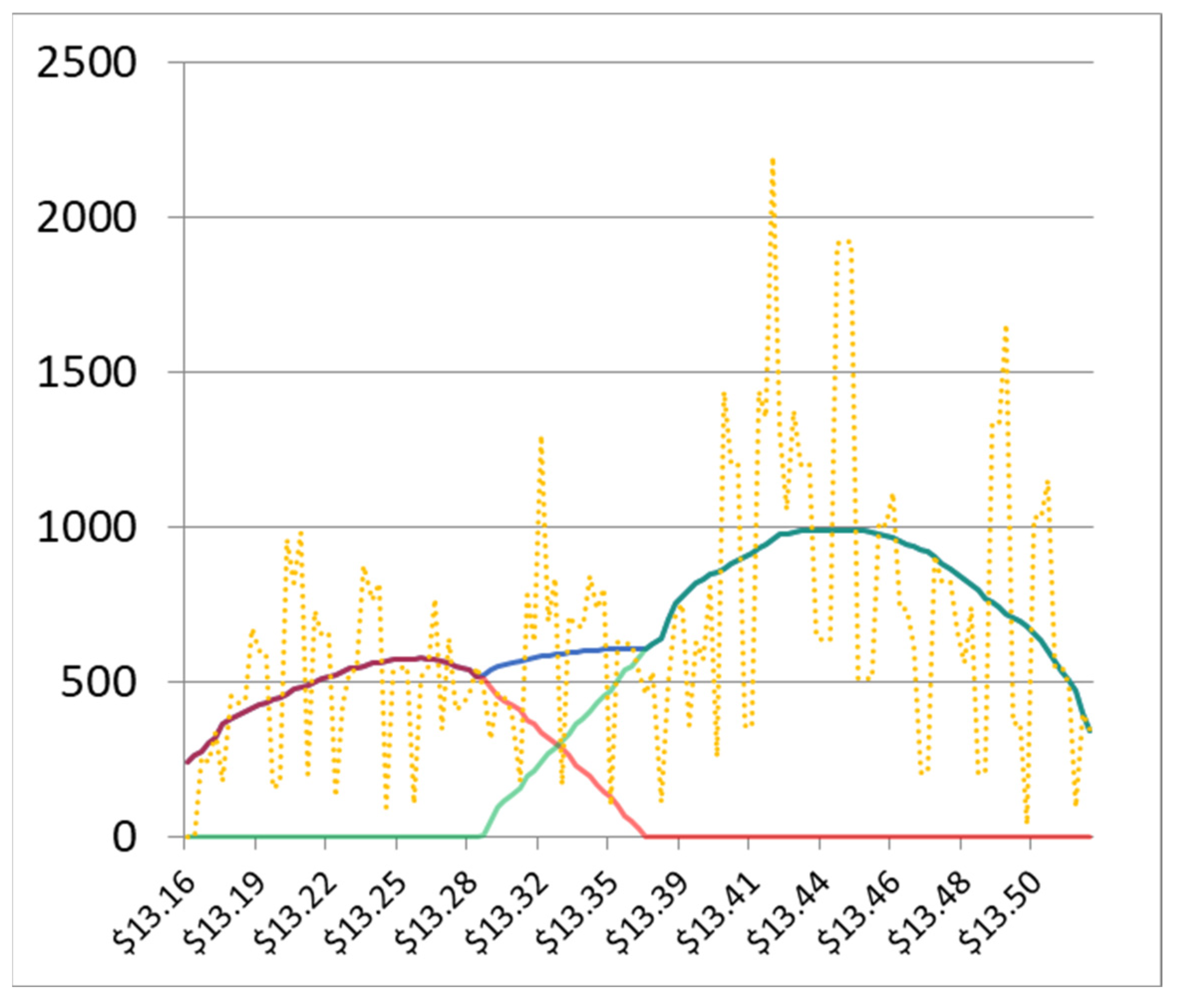
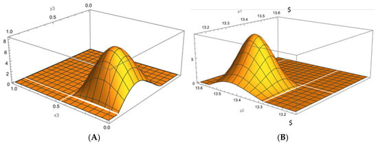
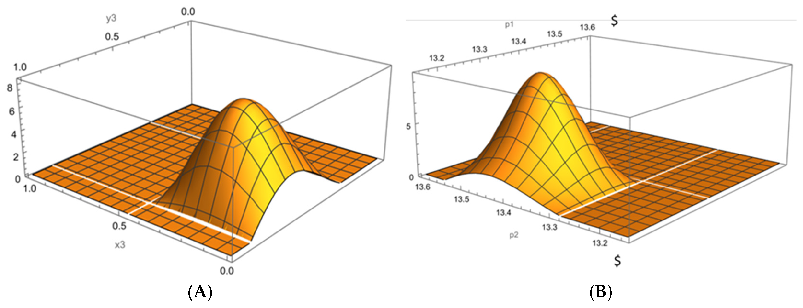
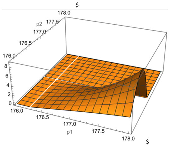
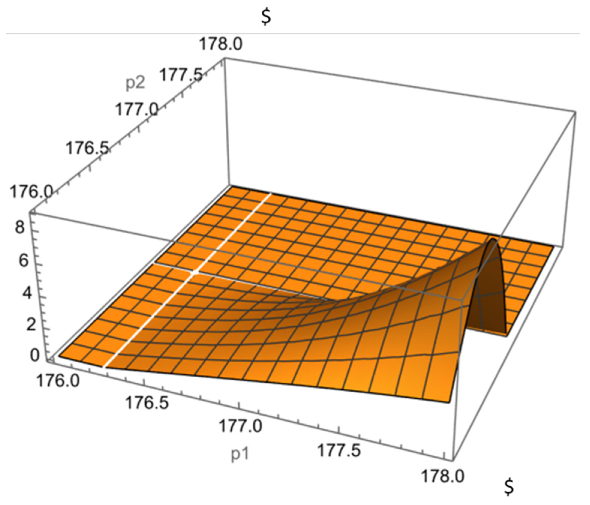
Empirical distributions and their estimates are plotted in Figure 1, Figure 2 and Figure 3. Visual comparison of the natural copula and some popular copula distributions (product, Gumbel, maximum correlation), as well as the pseudocodes are provided in Supplemental Materials and Graphics.
Figure 1.
Volume-at-Price distribution (yellow dot) for the IBM stock on 3 May 2016. The solid red line indicates our approximation of offers, the solid green line is the approximation of bids, and the blue curve is the sum of the total.
Figure 2.
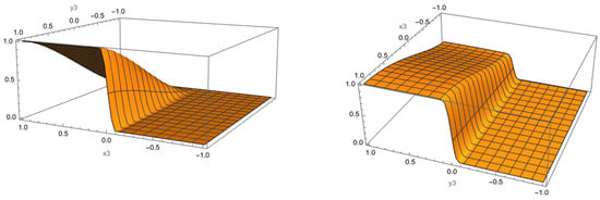
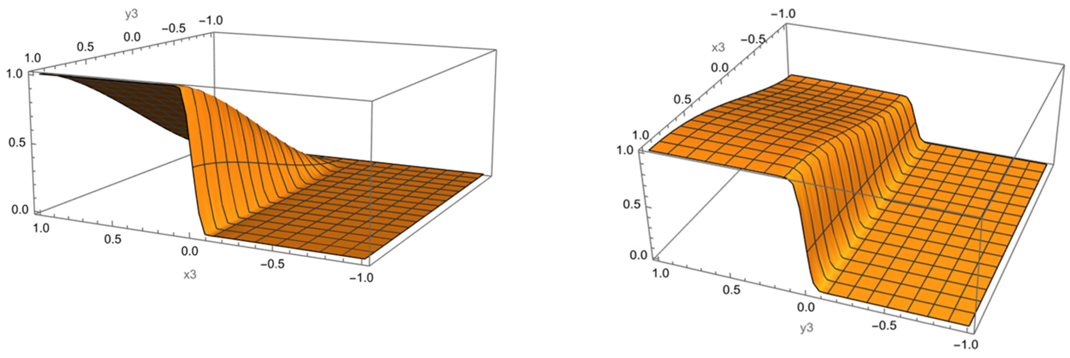
The density of the natural copula of the IBM Volume-at-Price (VaP) distribution in (A) normalized coordinates, and (B) original dollar prices. The vertical scale is arbitrary.
Figure 3.
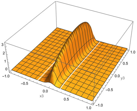
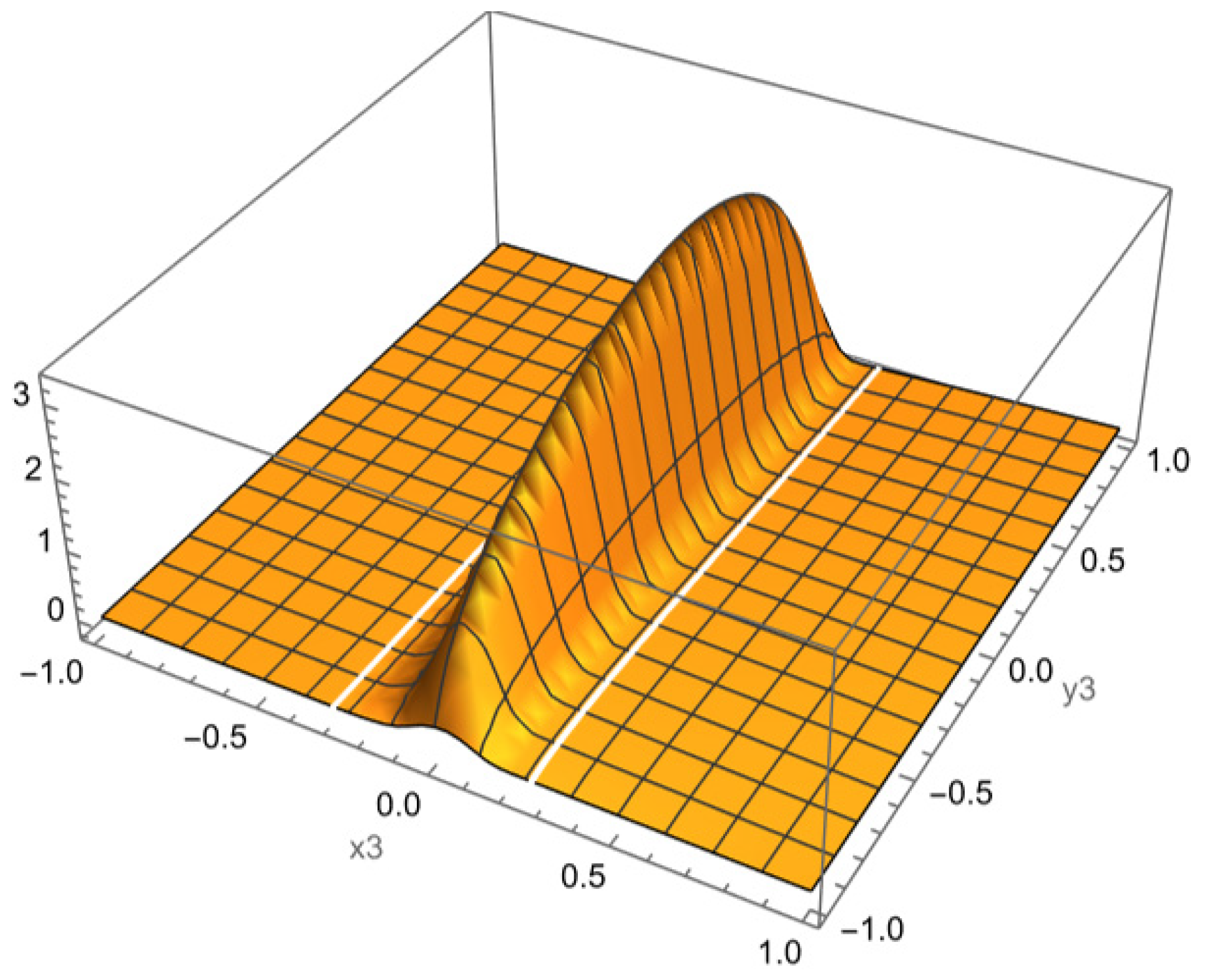
The density of a natural copula of a sample LOB of SPDR500.
7. Implicit Measure of Correlation
The measure of correlation, which is usually invoked in connection with copulas, is the Kendall copula tau parameter (Shemyakin & Knyazev, 2017). One possible extension of the concept of correlation to our method of estimation is the following expression:
For the factorizable distributions, the expression of Equation (7) is zero by construction. The estimates of our two model distributions are given in Table 3 and Table 4. The above correlation is independent of our copula approach and is a feature of the preferred method of estimation we outlined in Section 5.
Table 3.
The measure of correlation of Equation (10) for the normalized copulas. IBM designates a copula between IBM VAP daily distributions for buy and sale orders, and a copula between SDPR500 designates estimated LOB distributions for buy and sale orders.
Table 4.
The entropic measure of correlation of Equation (7′) for the normalized copulas. Estimated distributions are the same as in Table 3.
However, the application of the concept of correlation to copulas in general is not that straightforward. The correlation of copulas is not equivalent to the correlation of underlying stochastic processes. A high correlation embedded in copula construction means that the stochastic processes of the marginal distributions are similar in law. High correlation of the time series producing these distributions means that they are similar in probability, which is a much stronger condition. Entropic measures of distributions’ affinity might be more meaningful:
8. Gluing of the Copulas
The concept of the “natural copula” enables a hydrodynamic illustration in terms of conservation of probability (see Appendix A). Similarly to the flow of incompressible liquid, the distribution density remains equal to one (Villani, 2003, pp. 14, 29 for his definition of gluing). This hints at the following possibility. If we have three distributions, φ1(x), φ2(y), and φ3(z), and estimate the copulas U12(φ1(x), φ2(y)) and U23(φ2(y), φ3(z)) according to the prescriptions of Section 4, it is possible to construct a copula U13(φ1(x), φ3(z)) following straightforward rules.
Building on the analogy introduced in Section 7, we hypothesize that constructing a copula between two one-dimensional distributions is equivalent to determining the flow of an incompressible fluid between a source and a sink. Within this framework, it is possible to implement a transshipment through an intermediate pair of distributions (Rachev & Rüschendorf, 1998, p. 2; Villani, 2003, p. 11). In practical terms, this means that the terminal conditions of the first transport problem can be treated as the initial conditions for the second. By iteratively applying this procedure, the resulting flow defines a copula linking the first and third distributions.
This simple statement can be very useful for reducing computational complexity in the construction of multidimensional copulas. If we want to use binary copulas , i = 1, N, to construct a higher-dimensional copula, we need to make O(N2) estimations (see, e.g., Kojadinovic & Yan, 2011). However, employing the gluing procedure and creating a vocabulary with a standard distribution, for instance, uniform, the number of necessary estimations will be only linear in N.
We used returns on the five ETFs that invest in bonds of ESG-compliant companies (see the list in Appendix B). This choice is more or less arbitrary. We use it to emphasize the fact that one of the most frequent uses of copulas in finance is the determination of VaR and similar metrics for investment portfolios (Brigo et al., 2010; Cherubini et al., 2016).
A popular method of construction of multivariate copulas is the so-called method of vine copulas (Nelsen, 2006; Shemyakin & Knyazev, 2017). To build a vine copula for the test portfolio of five assets, we first produced three-dimensional copulas. This is done according to the following formulas for the PDFs.
We can check by direct computation that
In Equation (8), i, j, k = 1, 2, …, 5, I, J, K = 1, 2, …, 5. Lowercase letters index the coordinates; uppercase letters index the distributions obtained at the first stage of the estimation F(.). Because of the functional form of Equation (11), instead of I × J × K = 125 combinatorial options, we need to estimate only distributions.
It turned out that the Gaussian–Hermite basis of Table 1 was not optimal.2 A spline approximation worked better. Furthermore, a “natural” standard distribution turns out to be the Wigner distribution , which plays the role of normal distribution in the free probability theory (Voiculescu et al., 2016; Mungo & Speicher, 2017). The reason for this will be the subject of further investigation.
A functional form of Equation (4) also turned out not to be optimal for numerical estimation. Instead, we used the following trial functions for the pairs of CDFs:
In Figure 4, we demonstrate the construction of a binary copula of two empirical distributions from copulas of each of the empirical distributions (F12[x,y], F21[x,y]) with a Wigner distribution:
Figure 4.
Estimated CDFs for the gluing procedure for the returns of the ESGS and ETHO ETFs (see Appendix A) in the period 5 December 2023–5 October 2024.
The functional form in Equation (10) is suggested by the unnumbered equation in Rachev and Rüschendorf (1998, Theorem 1.4.11).
Wigner distribution can be restored from a cross-section of the three-dimensional copula in Figure 5.
Figure 5.
The cross-section of the three-dimensional distribution obtained by the procedure of Section 8 for the ESGS-ETHO ETF. We observe that it recovers the Wigner semi-circular distribution.
Summing up the contents of this section, our gluing construction is a version of the vine copula, in which one uses an unspecified but standard vocabulary of the functional forms. Hence, the marginals are estimated only once during the numerical procedure. This advantage does not seem critical for the relatively low-dimensional copulas provided here as an example, but it can be critical in cases where the dimensionality curse arises.
9. Multivariate Copulas
To produce a natural multivariate copula from one-dimensional distributions, we can use the method of the vine copula described, for instance, in (Czado, 2019). We have chosen a portfolio of five assets, namely the returns of ESG-themed Exchange Traded Funds (ETFs). The list of funds is provided in Appendix A.
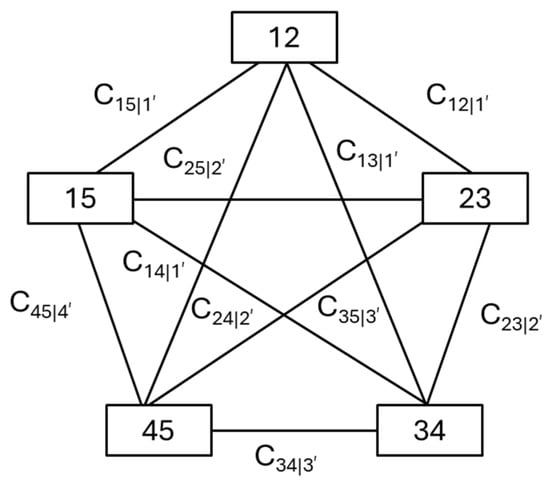
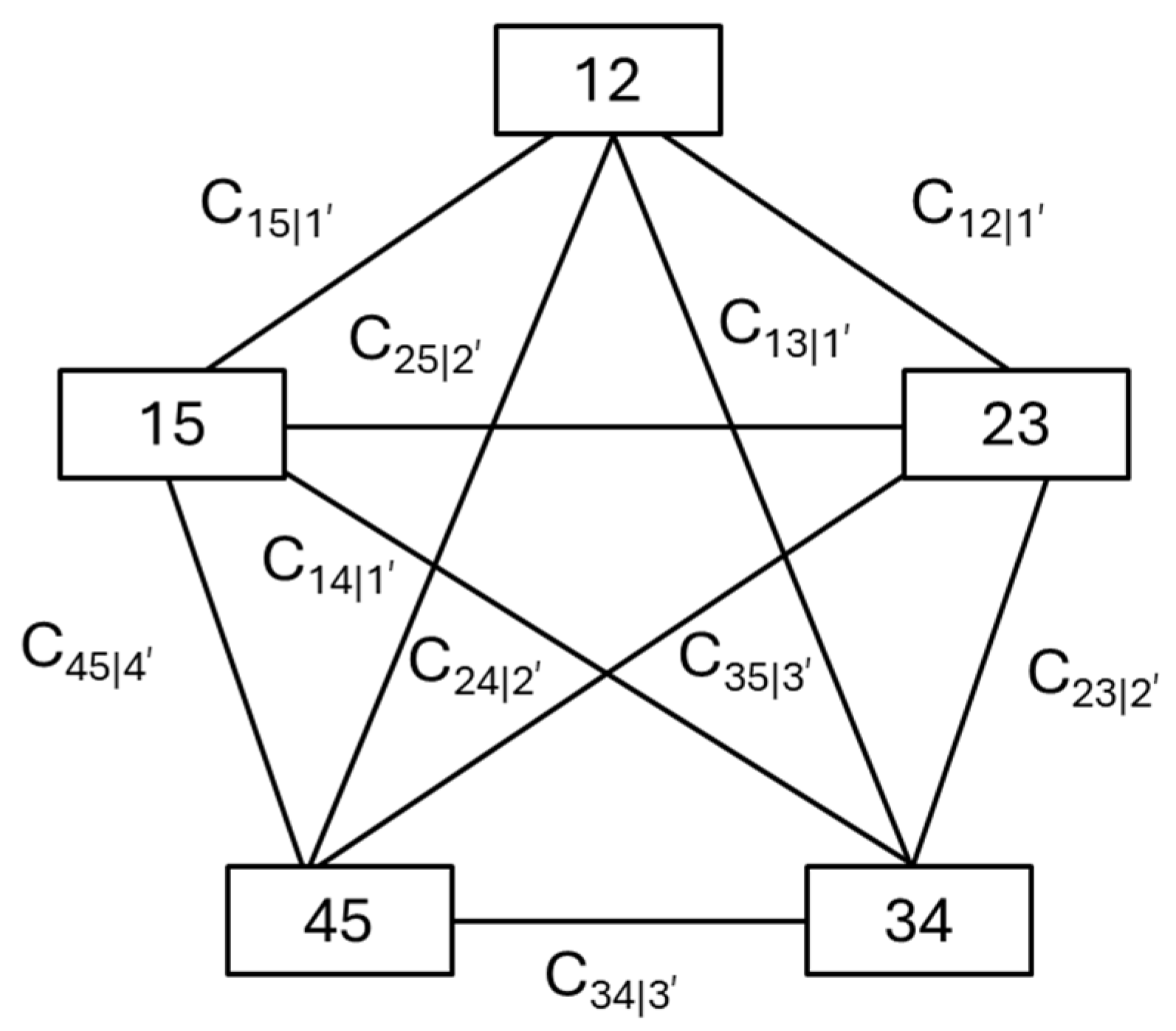
If we limit ourselves to the second third-degree dependencies between the returns, according to (Shemyakin & Knyazev, 2017), the vine formula for the five-dimensional copula will be
In Equation (11), f(xi) are the marginal distributions for the variables i = 1, 2, …, 5, and Cij|k are the three-dimensional correlations obtained from Equation (11). The factors Cij|k are conditional distributions of the variables i and j, f(xi, xj), for the value of variable k equal to xk.
We present the construction scheme for the five-dimensional copula in Figure 6.
Figure 6.
Vine diagram for the five-dimensional copula in the 3-fund approximation (i.e., correlations between four tuples of funds are ignored). The numbers correspond to the ordinal of the asset in Appendix A.
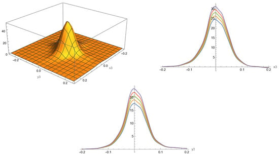
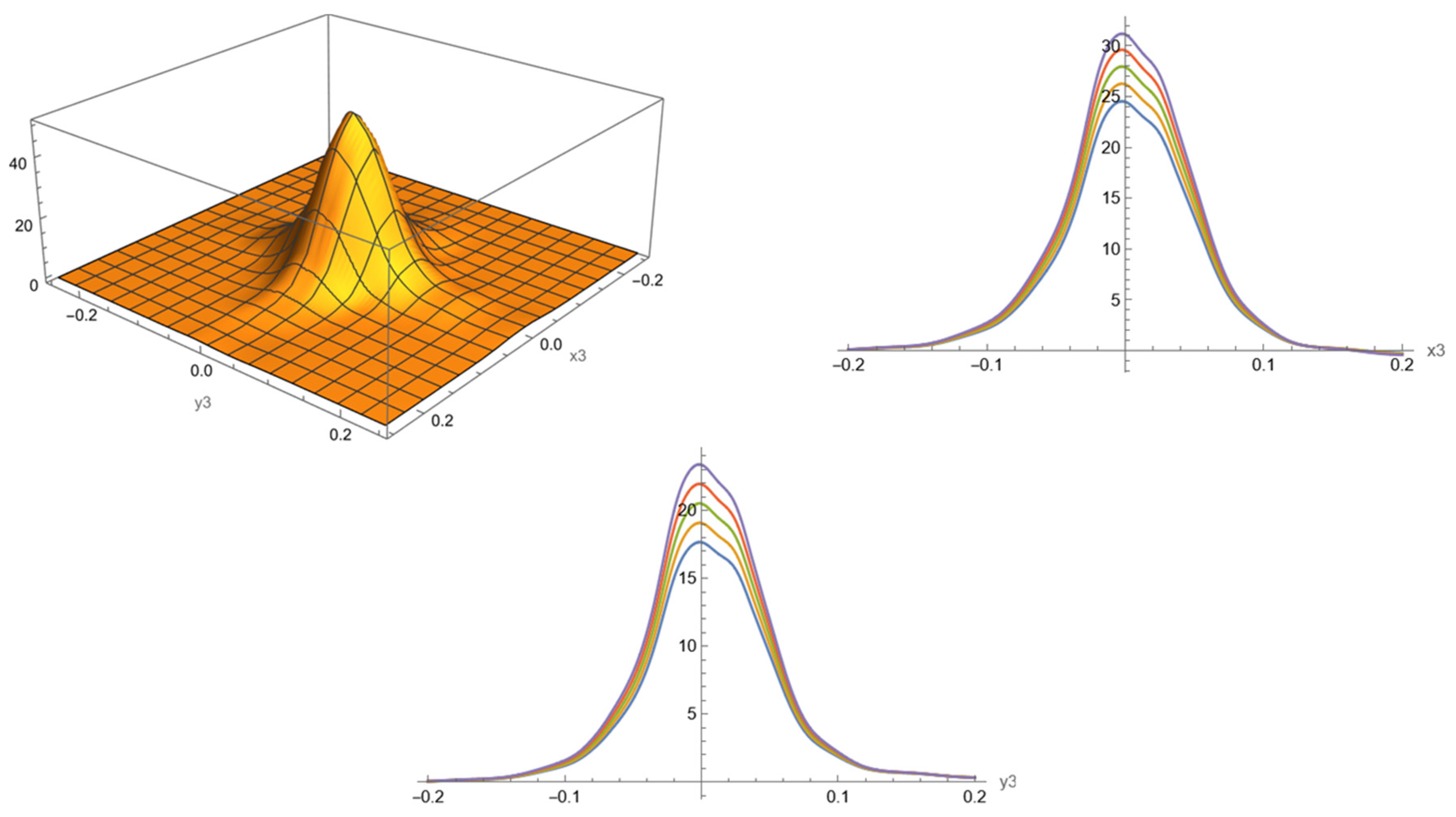
Because a six-dimensional manifold (five independent and one dependent variable) cannot be conveniently plotted on a two-dimensional sheet, we demonstrate only the cross-sections along the plane of ESGS-ETHO funds in Figure 7.
Figure 7.
Two-dimensional and one-dimensional cross sections (X-Z and Y-Z planes) of the copula for the returns of the five funds in Appendix A. Only funds 1 and 2 in Table A2 are plotted. Colored curves correspond to the simulated analysis of reaction of funds 1 (ESGS, upper plot) and 2 (ETHO, lower plot) to the changes in the returns of the third fund (KARS). The curves begin with −25 bp change of returns of the fund 3 with the step of 5 bp from color blue (−25 bp) to purple (0 bp), respectively.
One cannot ascertain whether the copula constructed in this way minimizes the Wasserstein distances between one-dimensional distributions, even neglecting dependencies of the four assets, exclusively from Equation (11). To clarify this issue, we employ the Kolmogorov–Arnold neural network (KAN).
10. Kolmogorov–Arnold Network
Why use copulas when neural networks can approximate the empirical results well? Unlike the original dataset, the copula generated by the algorithm in Figure 6 can be decomposed into constituent parts and used for prediction and risk analysis. A typical question in the risk analysis context is the following: What will the expected returns of stocks A and B be if stock C falls by 3%? Note that the last data point can be within or outside the historical dataset.
According to the famed representation theorem of Arnold and Kolmogorov, any multivariate function can be expressed as a composition of functions of only three variables using two operations: composition and addition (Kolmogorov, 1956; Arnold, 1957).
The original version of the theorem speaks of the finite number of compositions. However, the universal Kolmogorov–Arnold representation was reduced to increasingly parsimonious forms, culminating in the simplest (see Sprecher, 1965; Braun, 2010), namely a combination of two functions with appropriate dilations and shifts.
This form of the K-A theorem using shifts is especially useful in constructing a KAN on the functional basis of marginals. We use the Mathematica© version of the KAN designed by Hafver (2008). Unlike a multi-layer perceptron neural network (NN), which uses fixed activation functions on nodes and learnable weights on edges, the KAN uses algebraic summation on nodes and learnable activation functions on edges.
As is the problem with all NNs, it is difficult to assess multidimensional tensors, which are typically their output, from a human perspective. To use the KAN, we use the following pre-processing procedure. First, we create training files from the discrete numeric output of the three-dimensional copulas of Section 8 (five basis functions). Second, we use a ten-dimensional vector of empirical ETF returns as a test file. The logic of doing so is as follows.
We force the KAN to accept our functions as primary data. The network uses its own (black box) criteria to fit the original data. In the end, we try to fit a five-dimensional array of actual ETF returns with our combination of ten standard functions.
Because neural networks typically rely on an implicit metric or pseudo-metric—such as mean squared error or Kullback–Leibler divergence—we hypothesize that the resulting approximation is near-optimal with respect to the Wasserstein distance. We emphasize that this remains a conjecture: we do not claim that Kolmogorov–Arnold networks (KANs) produce solutions that are optimal in the strict sense of transport theory. Rather, we suggest that their solutions are likely to be close to optimal.
This expectation arises from a key structural difference between KANs and standard neural networks. While conventional networks adjust the weights of perceptrons, KANs keep these weights fixed and instead adapt the activation functions locally. As noted by Z. Liu et al. (2024), KANs demonstrate a superior ability to approximate special functions (Section 3.2) as well as solutions to elliptic differential equations (Section 3.4). Since the nonlinear equations encountered in transport theory are typically degenerate elliptic (Rachev & Rüschendorf, 1998), it is reasonable to expect that the advantages of KANs extend to our setting.
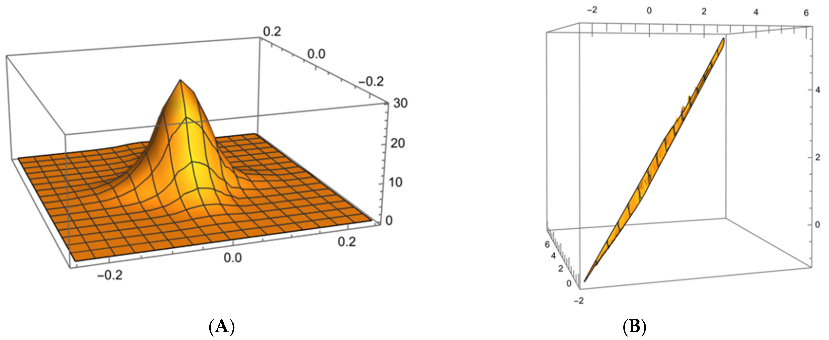
Furthermore, Rüschendorf’s (1985) Theorem 2 establishes that, under mild regularity conditions, the Wasserstein distance admits an analytic representation. Because the splines used in KAN were explicitly designed to approximate analytic functions, this suggests that numerical approximations based on KANs—particularly those employing spline-based representations of underlying analytic structures—can achieve high accuracy. We expect the cross-sections of the output data to be the results of linear transformation of their arguments, thus making Jacobian simply a number. The results of the KAN are shown in Figure 8. This suggests that the fitting of the three-asset pools of our five-asset portfolio to the vine Equation (11) was successful.
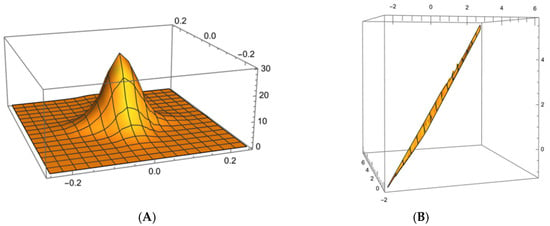
Figure 8.
(A) A two-dimensional cross-section of the empirical copula obtained by KAN. (B) Neural network regression of the empirical copula on the copula obtained by the approximate algorithm of Section 9. A narrow diagonal from the lower plane of the XYZ cube to the upper plane reflects good quality of approximation.
11. Conclusions
This paper demonstrates that a natural copula is the one that minimizes the Wasserstein distance between probability distributions within a common embedding space. Its estimation involves no arbitrariness beyond the choice of this embedding space and the order of the Wasserstein distance. In most applications, the embedding space and approximation metrics arise naturally from the problem setting.
Historically, questions of priority in the development of copula theory date back to the 1940s and 1950s, and we do not claim that the present construction is entirely novel. Nevertheless, the combination of numerical and conceptual advantages explored here—namely, the use of independently estimated marginals as priors (see also Genest et al., 1995), linear programming for estimation, standard distributional frameworks, the hydrodynamic interpretation of probability flow in the sense of Arnold–Brenier, and direct applicability to problems of financial relevance—suggests that unifying these elements under the framework of Wasserstein geometry is both natural and instructive.
The proposed estimation method, based on linear programming, is fully nonparametric and does not rely on any specific functional form of the copula. Moreover, the natural copula admits an intuitive hydrodynamic interpretation: if one distribution is viewed as a source and the other as a sink, the transport of probability mass between the marginals follows the Euler equations. In this analogy, incompressibility corresponds to the preservation of total probability (i.e., normalization).
Extending the concept of a natural copula to higher dimensions presents additional challenges. As an approximation, we employ vine copulas, which significantly reduce the computational complexity of multivariate estimation. To further investigate this issue, we apply Kolmogorov–Arnold neural networks (KANs). Our findings suggest that, for five assets, a three-asset vine copula provides a reasonable approximation to the fully empirical copula produced by the “black box” of a neural network.
The convergence of empirical copulas to the true underlying distribution has been extensively studied and established under various conditions (e.g., Fermanian et al., 2004; Radulovic et al., 2017 and op. cit.). This body of work supports the use of semi-empirical approaches to copula construction, even in higher-dimensional settings. The treatment of very-high-dimensional cases remains an important direction for future research.
Supplementary Materials
The following supporting information can be downloaded at: https://www.mdpi.com/article/10.3390/econometrics14020027/s1.
Funding
This research received no external funding.
Data Availability Statement
Supplementary Material contains pseudocodes and visual comparisons of copulas. Further inquiries can be directed to the corresponding author.
Conflicts of Interest
The author declares that the research was conducted in the absence of any commercial or financial relationships that could be construed as a potential conflict of interest.
Appendix A. Hydrodynamic Interpretation of the “Natural Copula”
The connection of the problems of optimal transport with hydrodynamics evolved from the pioneering 1960s work by Arnold (1966) and was resuscitated in the 2000s through the work of Benamou and Brenier (see Brenier, 2004 and op. cit.) (for the modern bibliography, one can consult J.-G. Liu et al., 2019 and Chizat et al., 2018). Approximately, the Wasserstein distance between two shapes/distributions is minimized by the flow of an incompressible fluid that obeys the Euler equations. Heretofore, we can assume that one marginal distribution is a hydrodynamic source and the other is a drain for an incompressible fluid. Incompressibility preserves the normalization of the distributions of probability flows. The properties of a natural copula are thus related to the global properties of probability flow.
We illustrate this interpretation by plotting the vector field associated with the derivatives of the copula function in Figure A1. We interpret these derivatives as velocities:
where V(x,y) is a potential function of the flow, which we identify with our copula. Then, as usual, we can define the following characteristics:
which are called circulation and flux in hydrodynamics. We choose the contour of integration along the border of the sampling area. Because of the square integration region [0, 1] × [0, 1], the y-integrals over parts of the integration contour parallel to the x-axis and the x-integrals over contour intervals parallel to the y-axis are identically zero (see Figure A1). So, only one component of flow velocity gives a contribution to the contour integral:
The results of our calculation, expressed in arbitrary units, are provided in Table A1.
Figure A1.
Hydrodynamic velocity vector fields of copula distributions. (A) Vector field corresponding to the copula distribution in Figure 2A of the main text. Arrows indicate the magnitude and direction of hydrodynamic velocities (Equation (A1)). (B) Vector field corresponding to the copula distribution in Figure 3B of the main text. Arrows indicate the magnitude and direction of hydrodynamic velocities (Equation (A1)).The coordinates x and y are the percentage scales of the embedding box [0, 1] × [0, 1].
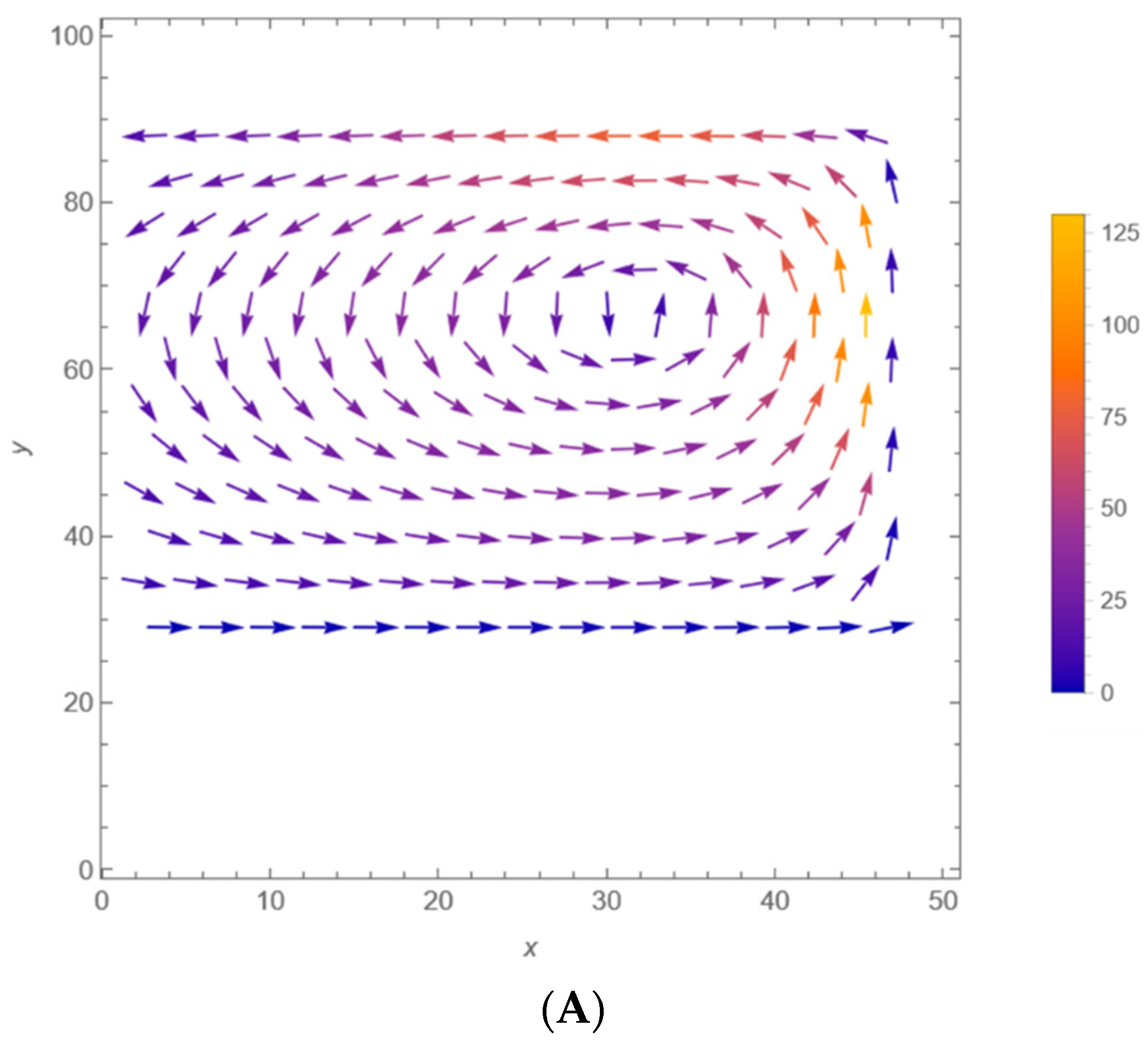
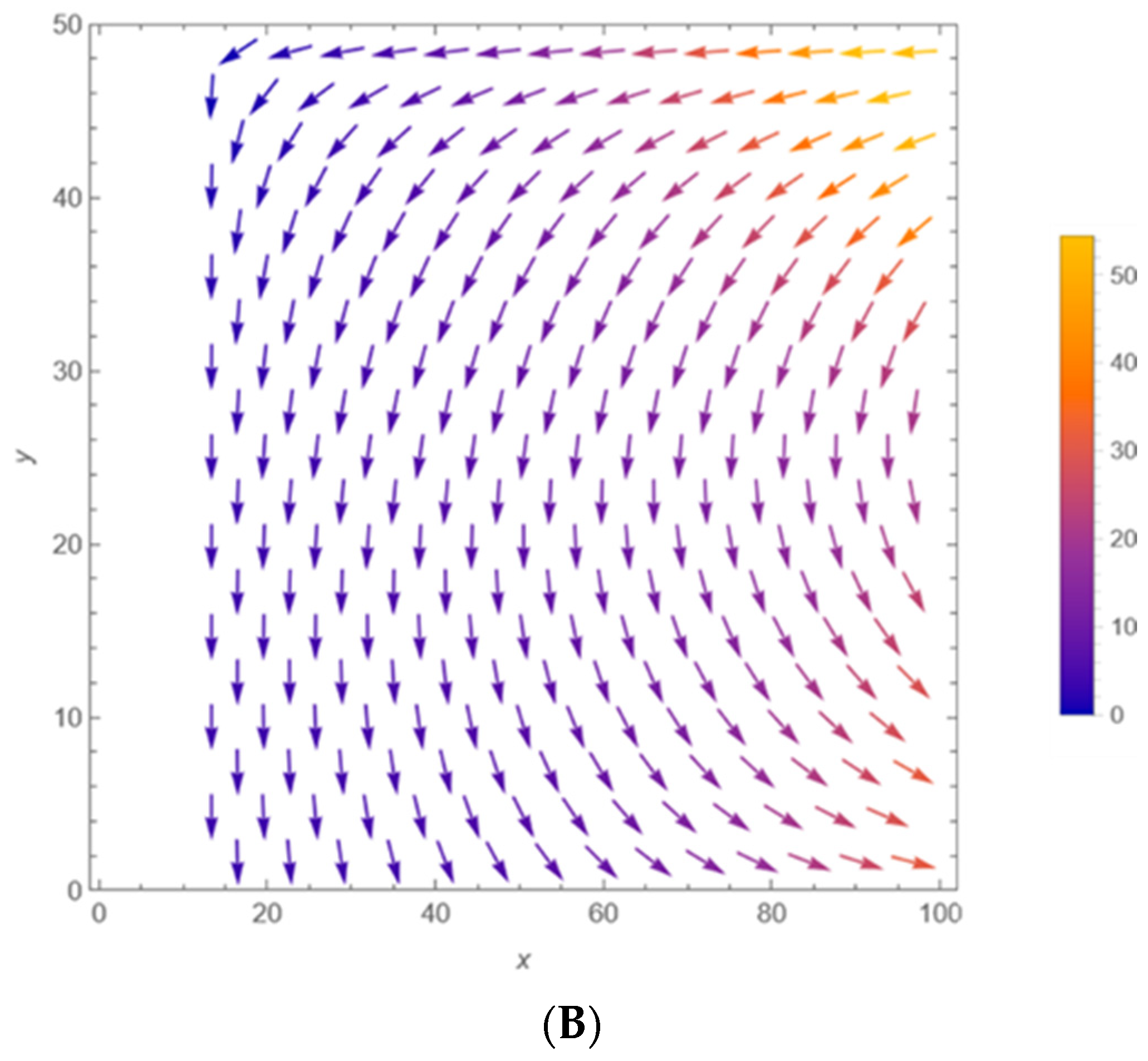
Table A1.
Hydrodynamic flux Φ and circulation Γ (Equation (6)) for the sample copulas in arbitrary units. Turnover is significant, while the imbalance is small 1.
We tentatively identify circulation with the number of shares changing hands in the case of optimal unwinding of the LOB and flux with the market imbalance.
Appendix B. Description of the Funds’ Data Collection
Table A2.
Description of the Exchange-Traded Funds (ETFs) used for the multivariate sample in Section 8, Section 9 and Section 10 *.
Notes
| 1 | Note that the normalization condition uniquely determines the constant. |
| 2 | Optimality criteria included the speed and quality of convergence, among others, which may be portfolio-specific. For instance, in using a uniform distribution instead of Wigner’s semi-circular distribution, one must smooth the corners of the PDF for the numerical estimation. |
References
- Abdelatif, M., Kuchling, P., Rudiger, B., & Ventura, I. (2024). Wasserstein distance in terms of the comonotonicity copula. arXiv. [Google Scholar] [CrossRef] [Scilit]
- Abramowitz, M., & Stegun, I. (1964). Handbook of mathematical functions with tables, graphs and mathematical tables. NBS.
- Alfonsi, A., & Jourdain, B. (2014). A remark on the optimal transport between two probability measures sharing the same copula. Statistics and Probability Letters, 84, 131–134. [Google Scholar] [CrossRef] [Scilit]
- Arnold, V. (1957). On functions of three variables. Proceedings of the USSR Academy of Sciences, 114(4), 679–681. [Google Scholar]
- Arnold, V. (1966). Sur la geometrie differentielle des groupes de Lie de dimension infinie et ses applications a l’hydrodynamique des fluides parfaits. Annales de l’institut Fourier, 16, 319–361. [Google Scholar] [CrossRef] [Scilit]
- Braun, J. (2010). On Kolmogorov’s superposition theorem and its applications. Springer. [Google Scholar]
- Brenier, Y. (2004). Extended Monge-Kantorovich theory. In Optimal transportation and applications (pp. 91–121). Lecture Notes in Mathematics, 1813. Springer. [Google Scholar]
- Brigo, D., Pallavicini, A., & Torresetti, R. (2010). Credit models and the crisis: A journey into CDOs, copulas, correlations and dynamic models. Wiley & Sons. [Google Scholar]
- Cherubini, U., Gobbi, F., & Mulinacci, S. (2016). Convolution copula econometrics. Springer. [Google Scholar]
- Chizat, L., Peyre, G., Schmitzer, B., & Vialard, F.-X. (2018). Unbalanced optimal transport: Dynamic and kantorovich formulation. Journal of Functional Analysis, 274(11), 3090–3123. [Google Scholar] [CrossRef] [Scilit]
- Czado, C. (2019). Analyzing dependent data with copulas (Vol. 222). Springer. [Google Scholar]
- Durante, F., & Seupi, C. (2016). Principles of copula theory. CRC Press. [Google Scholar]
- Embrechts, P., & Hofert, M. (2013). Statistical inference for copulas in high dimensions: A simulation study. ASTIN Bulletin: The Journal of the IAA, 43(2), 81–95. [Google Scholar] [CrossRef] [Scilit]
- Fermanian, J.-D., Radulovic, D., & Wegcamp, M. (2004). Weak convergence of empirical copula processes. Bernoulli, 10(5), 847–860. [Google Scholar] [CrossRef] [Scilit]
- Fréchet, M. (1951). Sur les tableux de correlation dont les marges sont donnees. Annales de l’Université de Lyon. 3e série, Sciences Section A, 14, 53–77. [Google Scholar]
- Genest, C., Ghoudi, K., & Rivest, L.-P. (1995). A semiparametric estimation procedure of dependence parameters in multivariate families of distributions. Biometrika, 82(3), 543–552. [Google Scholar] [CrossRef]
- Hafver, A. (2008). Wolfram community. DNV. [Google Scholar]
- Hasbrouck, J. (2007). Empirical market microstructure: The institutions, economics and econometrics. Oxford UP. [Google Scholar]
- Hoeffding, W. (1940). Masstabinvariante Korrelationstheorie. Schrifften des Matemathisches Instituts and Instituts fuer Angewandte Mathematic der Universitaet Berlin, 5, 181–233. [Google Scholar]
- Hofert, M., & Scherer, M. (2011). CDO pricing with nested Archimedean copulas. Quantitative Finance, 11(5), 775–787. [Google Scholar] [CrossRef] [Scilit]
- Joe, H. (1997). Multivariate models and dependence concepts. Chapman & Hall. [Google Scholar]
- Kantorovich, L. (1942). On the translocation of masses. Doklady Akademii Nauk SSSR, 37, 199–201. [Google Scholar] [CrossRef] [Scilit]
- Kim, G., Silvapulle, M. J., & Silvapulle, P. (2007). Comparison of semiparametric and parametric methods for estimating copulas. Computational Statistics & Data Analysis, 51, 2836–2850. [Google Scholar] [CrossRef] [Scilit]
- Kojadinovic, I., & Yan, J. (2011). A goodness-of-fit test for multivariate multiparameter copulas based on multiplier central limit theorems. Statistics and Computing, 21, 17–30. [Google Scholar] [CrossRef] [Scilit]
- Kolmogorov, A. (1956). On the representation of continuous functions of several variables by superpositions of continuous functions of a smaller number of variables. Proceedings of the USSR Academy of Sciences, 179–182. [Google Scholar]
- Lax, P. (2002). Functional analysis (Pure and applied mathematics: A Wiley series of texts, monographs and tracts). Wiley. [Google Scholar]
- Liu, J.-G., Pego, R. L., & Slepcev, D. (2019). Least action principles for incompressible flows and geodesics between shapes. Calculus of Variations and Partial Differential Equations, 58, 179. [Google Scholar] [CrossRef] [Scilit]
- Liu, Z., Wang, Y., Vaidya, S., Ruehle, F., Halverson, J., Soljacic, M., Hou, T., & Tegmark, M. (2024). KAN: Kolmogorov-Arnold Networks. arXiv. [Google Scholar] [CrossRef] [Scilit]
- Matousek, J., & Gartner, B. (2007). Understanding and using linear programming. Springer. [Google Scholar]
- Monge, C. (1781). Memoire sur la theorie des deblais et des remblais. Histoire de l’Academie Royale des Sciences de Paris. [Google Scholar]
- Mungo, J. A., & Speicher, R. (2017). Free probability and random matrices (Vol. 35). Fields Institute Monographs. Springer. [Google Scholar]
- Nelsen, R. B. (2006). An introduction to copulas. Springer. [Google Scholar]
- Rachev, S. T., & Rüschendorf, L. (1998). Mass transportation problems (Vol. 1). Springer. [Google Scholar]
- Radulovic, D., Wegcamp, M., & Zhao, Y. (2017). Weak convergence of empirical copula indexed by functions. Bernoulli, 23(4B), 3346–3384. [Google Scholar] [CrossRef] [Scilit]
- Rüschendorf, L. (1985). The Wasserstein distance and approximation theorems. Probability Theory and Related Fields, 70, 117–129. [Google Scholar] [CrossRef] [Scilit]
- Rüschendorf, L. (Ed.). (1996). Development of Frechet-bounds distributions with fixed marginals and related topics. In Risk bounds and partial dependence information (Vol. 28, pp. 345–346). Springer. [Google Scholar]
- Shemyakin, A., & Knyazev, A. (2017). Intorduction to Bayesian estimation and copula model of dependence (A. Knyazev, & A. Shemyakin, Eds.). Wiley & Co. [Google Scholar]
- Sklar, A. (1959). Fonctions de repartition a n dimensions et leur marges. Publications de l’Institute de Statistique de l’Universite de Paris, 8, 229–231. [Google Scholar]
- Sklar, A. (1960). Random variables, joint distribution functions, and copulas. Kybernetica, 9(6), 449–460. [Google Scholar]
- Sprecher, D. (1965). On the structure of continuous functions of several variables. Transactions of the American Mathematical Society (AMS), 115, 340–355. [Google Scholar] [CrossRef]
- Villani, C. (2003). The Wasserstein distances. In Topics in optimal transportation. American Mathematical Society. [Google Scholar]
- Voiculescu, D. V., Stammeier, N., & Weber, M. (Eds.). (2016). Free probability and operator algebras. Munster Lectures in Mathematics. EMS. [Google Scholar]

Disclaimer/Publisher’s Note: The statements, opinions and data contained in all publications are solely those of the individual author(s) and contributor(s) and not of MDPI and/or the editor(s). MDPI and/or the editor(s) disclaim responsibility for any injury to people or property resulting from any ideas, methods, instructions or products referred to in the content. |
© 2026 by the author. Licensee MDPI, Basel, Switzerland. This article is an open access article distributed under the terms and conditions of the Creative Commons Attribution (CC BY) license.