


Abstract
Mobile platforms such as high-speed trains and unmanned aerial vehicles (UAVs) experience quasi-periodic variation in link quality as they move through a cellular base-station lattice, so the service rate of their on-board uplink buffer is itself time-periodic. We model this buffer as a periodic queue whose service rate follows from a signal-to-noise-ratio (SNR)-to-rate map and construct an edge-resident controller that exploits this periodic structure for real-time quality-of-service (QoS) control. From a harmonic-balance (Fourier–Galerkin) solution of the periodic regime, the controller derives backlog and tail-probability indicators and uses them to drive admission, redundancy and handover decisions on the device. The method rests on a stability criterion and a quantitative error bound for the spectral truncation, under stated regularity and stability conditions, and is validated against Monte Carlo simulation along a ∼650 km geo-anchored corridor: on the periodic backbone, the solver matches simulation to within about , and a coefficient-driven admission rule lowers the 99th-percentile delay by about relative to a reactive baseline at high load. On the full map-derived profile with aperiodic coverage gaps, the proposed proactive controller—spectral backbone admission combined with a radio-map look-ahead—attains the lowest mean and tail delay, about and below the reactive baseline and and below uncontrolled DropTail, with buffer overflow cut from to , at a deliberate admitted-load cost (goodput ≈0.84 vs. ). An operation-count analysis indicates compatibility with sub-ms control deadlines on a Cortex-A55-class system-on-chip. The controller runs on the device itself, without cloud or GPU, and the architecture is realised in a granted patent; end-to-end hardware benchmarking and an extension to non-Poisson traffic are left for future work.
1. Introduction
High-speed trains, vehicular fleets, unmanned aerial vehicles and other mobile sensing platforms increasingly rely on public cellular infrastructure for uplink aggregation of on-board telemetry, video and control traffic [1,2]; a current panorama of railway-dedicated 5G/6G systems is given in [3]. Outside dense urban areas, the inter-site distance between base stations (BSs) can exceed the kilometre scale, producing coverage gaps and strongly time-varying link quality along a route. Under near-constant-speed motion, the large-scale path loss experienced by an on-board aggregator is a spatially periodic function of the position relative to the BS lattice, which translates into a T-periodic signal-to-noise ratio (SNR) [4,5]. Since the achievable rate is a non-decreasing function of the SNR—in deployed systems a staircase map through the discrete modulation-and-coding schemes (MCS) [6], cf. Remark 1—the effective service rate at the aggregator is itself T-periodic, and the on-board queue must be analysed as a time-inhomogeneous birth–death process rather than a classical queue.
Traffic aggregation is a standard way to improve end-to-end performance on mobile platforms [7,8,9]: flows from multiple on-board clients are merged across all available links (5G/LTE, Wi-Fi, satellite) while the aggregator monitors channel quality and balances load (Figure 1). Existing link-aggregation standards, however, operate at the MAC/PPP layer and do not address cellular handover (Section Related Work); at 200–, LTE/NR mobility incurs frequent handovers and measurable extra latency [10,11,12,13]. A reasonable alternative is to buffer the load during low-SNR intervals rather than to trigger retransmissions that are likely to fail, in line with opportunistic and back-pressure scheduling [14,15,16,17].
Figure 1.
On-board traffic aggregation on a high-speed platform moving through a cellular base-station lattice. Heterogeneous sensors and actuators generate telemetry and control traffic (aggregate arrival rate ) into an on-board buffer; the consolidated flow is forwarded to the serving base station over a link whose service rate varies quasi-periodically with position, with handover in cell-overlap regions and a coverage gap (dead zone) between cells. An edge-resident spectral controller sets the admission factor from the backlog and tail indicators. Schematic illustration, not a measured deployment.
- Problem and scope.
To optimise on-device buffer control in this setting, one needs a model that couples three elements: (i) the spatially periodic large-scale path loss and the resulting SNR induced by the BS lattice; (ii) the vehicle speed, which sets the period T; and (iii) the queueing dynamics at the aggregator. We adopt an model in which Poisson arrivals of rate are served at a continuous T-periodic rate , obtained by mapping path loss to SNR and then to rate via Shannon’s formula as an information-theoretic upper bound [2,18]. This is the simplest model that retains both the periodic structure of the channel and the stochastic fluctuations of the traffic; finite-buffer theory and non-Poisson arrivals lie outside the analytical scope of the present paper, although finite-buffer effects are included in the simulation study of Section 5.
- Contributions.
The contribution of the present paper is threefold, concerning the system design, its mathematical foundation and its engineering feasibility.
System design (main contribution). We design and profile a spectral QoS controller for on-board mobile aggregators: a closed-loop pipeline (SNR → FFT → sparse SLAE → QoS metrics → TCP/FEC/HO actuation) that exploits the periodic structure of the radio environment to provide real-time delay and overflow control (Section 4). The controller presented here is the queueing-theoretic realisation of the on-board aggregator architecture protected by patent RU 2843669 C1 [19].
Mathematical foundation. The controller rests on the periodic queueing model driven by the physically motivated service profile . We restate the classical ergodicity criterion for periodic queues [20,21,22] (Theorem 1), prove geometric tail bounds for both the underloaded and the relaxed regime (Propositions 1 and 2), derive the harmonic-balance system and formulate a quantitative truncation error bound (Theorem 2), conditional on the weighted-regularity Assumption 1 and a uniform invertibility property (Assumption 2) that we verify numerically in Section 5, together with an explicit a posteriori error indicator usable by the controller at runtime. The multi-link Markov-modulated extension of the aggregation model is developed in [23].
Engineering feasibility. We profile the pipeline for a mid-class ARM Cortex-A55 system-on-chip using a worst-case operation-count analysis and show that representative truncation sizes fit comfortably within a scheduling period (Section 4); the entire loop is designed to run on-board without cloud assistance or GPU, constituting a lightweight, analytically grounded alternative to ML-based edge controllers such as [24]. Throughout, “edge-deployable” refers to a design whose worst-case operation count and memory footprint are shown to fit the runtime budget of a mid-class embedded SoC (Section 4; it does not claim a completed hardware deployment. An end-to-end hardware benchmark of the integrated controller is left for future work. To the best of our knowledge, the present paper is the first to use a spectral (Fourier–Galerkin) decomposition of a periodic queueing model as the computational kernel of an edge-resident QoS controller, with an operation-count budget estimated to be compatible with realistic embedded hardware (Section 4).
- Paper organisation.
Section 2 formalises the periodic channel model and the resulting system. Section 3 states and proves the ergodicity criterion (Theorem 1), develops the harmonic-balance system together with the truncation bound (Theorem 2), treats the small-modulation example and relates the model to the periodic fluid limit (Appendix E). Section 4 describes the on-device spectral controller and its profiled embedded implementation. Section 5 presents the numerical validation. Section 6 summarises the findings and outlines extensions.
Related Work
Modelling efforts relevant to high-mobility aggregation fall into five thematic strands.
- (A)
- Connectivity and coverage abstractions.
Percolation and stochastic-geometry models characterise large-scale connectivity and coverage of wireless networks but typically abstract away queueing dynamics and buffer control; see, for example, [25,26,27]. These models are complementary to ours: they set the coverage budget under which a periodic service profile is meaningful but do not address the latency induced by the resulting queue.
- (B)
- Markov-modulated wireless links.
Finite-state channel models obtained by discretising SNR into modulation-and-coding-scheme (MCS) levels yield Markov or semi-Markov descriptions and are widely used in embedded implementations [28,29]. The canonical burst-error model is the Gilbert–Elliott process [30,31]. More expressive driving processes are provided by the Markovian Arrival Process (MAP) and the Batch MAP (BMAP) of Lucantoni [32], which admit matrix-analytic stationary analysis. Relative to this line of work, our model replaces Markov modulation by a deterministic T-periodic service profile tied explicitly to the physical path loss. The two approaches are complementary: MAP/BMAP suits routes with genuine channel randomness, while a fixed BS lattice with a known speed profile is captured more parsimoniously by the periodic model and its spectral representation.
- (C)
- Non-stationary and periodic queues.
Non-stationary and periodic queues form an established subfield of queueing theory. Lemoine [20] and Heyman–Whitt [21] analysed time-varying birth–death systems via transient and drift methods; Massey–Whitt [33] and Margolius [22] studied the sample-path and asymptotic behaviour of periodic and systems, establishing the ergodicity criterion in its classical form. Harmonic-balance and Fourier-series expansions for the resulting periodic regimes appear, among others, in Kuczura [34] for small perturbations of and in Knessl–Yang [35] for asymptotic expansions of time-varying queues. The present work does not claim novelty for the ergodicity criterion or for the harmonic-balance technique as such; it contributes (i) a quantitative truncation error bound (Theorem 2) adapted to the specific block-tridiagonal structure of the physically motivated problem and (ii) a tight integration of the resulting spectral solver with an edge-deployable hardware pipeline. For the linear ODEs with periodic coefficients that underlie the truncated harmonic-balance system, we rely on the classical Floquet theory as presented in [36].
- (D)
- Handover and protocol-level studies.
Studies of high-speed mobility and handover focus on radio requirements and handover procedures [10,11,12]—see [3] for the state of the art in 6G-enabled railway systems—or on network-selection and aggregation policies [37], while the link-aggregation standards LACP and Multilink PPP are defined for MAC- or PPP-layer adjacency and do not address cellular handover dynamics [38,39]. These works frame the practical constraints within which our aggregator must operate but do not provide a queueing-theoretic model of the resulting buffer dynamics.
- (E)
- Edge-deployed queueing and control.
Recent research on edge-deployed traffic control for vehicular and high-speed scenarios combines measurement and prediction of channel state with adaptive buffering, typically via Kalman filtering [40] or compact neural predictors [41,42]. Such approaches are effective empirically but rely on learned surrogate models of rather than on a tractable analytical description. The closest antecedent to the controller developed here is the adaptive aggregator design of [7,19], to which we contribute an analytically supported and profiled spectral control loop.
- (F)
- Queue control at IoT edge nodes: ML approaches and alternatives.
A rapidly growing body of work addresses adaptive queue management at edge-IoT nodes. A recent study [24] proposes decentralised queue control with a parameterised service-time shift for a model, implemented via a DQN (Deep Q-Network) reinforcement-learning agent; the authors report a 17–26% reduction in average delay compared with DropTail/RED/CoDel on real-world edge-IoT traces. However, the approach requires training data and a non-trivial training/tuning cost, provides no formal convergence guarantee for the deployed policy and does not model the periodic structure of the service rate arising from physical propagation. Standard AQM heuristics (DropTail, RED [43], CoDel) do not adapt to a time-varying ; SDN-based QoS frameworks [44] are centralised and ill-suited to resource-constrained edge devices; and the L4S mechanism [45,46] targets time-critical 5G traffic without a queueing-theoretic model of periodic service modulation.
- (G)
- Prior work by the authors and patent protection.
The present work continues a research programme on mobile traffic aggregation by the authors. Kalimulina [47] proposed multi-valued logic models for traffic classification in mobile-network aggregation. Esin and Kalimulina [23] developed a Markov-modulated queueing network for mobile traffic aggregation with threshold-controlled buffers, which generalises the single-link model of the present work to a multi-link Markov-modulated setting. The adaptive aggregator architecture described in [7,19] is protected by Russian patent RU 2843669 C1 (published 17 July 2025); see the Conflicts of Interest statement.
- Gap addressed and novelty claims.
Relative to strands (A)–(G) above, the contribution of this work is at the intersection of three areas that have not been connected before:
- Spectral queueing method as a real-time control kernel. We use the harmonic-balance (Fourier–Galerkin) decomposition of the periodic queue not merely as an analytical tool but as the computational engine of an edge-deployed QoS controller. To the best of our knowledge, no prior work has deployed a spectral queueing solver on an embedded platform for real-time buffer management.
- End-to-end pipeline from physical propagation to actuator commands. The controller closes the loopwithin the profile-update budget of an on-board ARM Cortex-A55 SoC—the sparse solve runs at profile-update times, the online step being metric evaluation and thresholding—without cloud assistance (operation-count budget, Section 4), constituting a lightweight, analytically grounded alternative to ML-based edge controllers.
- Analytically grounded error control. The truncation error bound of Theorem 2—conditional on the weighted-regularity Assumption 1 and the numerically supported uniform-invertibility Assumption 2, and accompanied by the runtime a posteriori indicator —provides a quantitative handle on the accuracy of the spectral solver that neither heuristic (DropTail, RED, CoDel) nor purely learning-based (DQN [24]) controllers expose.
Table 1 summarises the comparison of the proposed spectral controller with the main competing approaches.
Table 1.
Comparison of the proposed spectral controller with competing edge-QoS approaches.
- Notation.
2. Problem Statement
We consider a high-mobility platform equipped with an on-board traffic aggregator that moves past a linear array of cellular base stations (BSs). Let the BS locations form a one-dimensional lattice with inter-site distance , and let the aggregator travel at an essentially constant speed along the lattice.
Because the received power depends on the instantaneous position relative to the nearest site, the achievable service rate varies periodically along the route. It is therefore natural to introduce the period
and the dimensionless intra-cell coordinate , which cycles once per inter-site interval. Passengers’ devices associate locally with the on-board aggregator; such single-hop, multi-interface architectures are standard in contemporary 4G/5G deployments and hide frequent handovers from end users [7,48,49].
We focus on the sparse-coverage regime: the inter-site distance is large enough to produce intervals where the SNR falls below an operational threshold, creating coverage gaps (“dead zones”). At the same time, mobility is high (typical rail/highway speeds), so multiple handovers can occur over application-level time horizons.
Our objective is to model the queue formed at the on-board aggregator under these conditions. We assume a Poisson aggregate input of rate and a single server whose service rate is a continuous, T-periodic function induced by the large-scale path-loss/SNR profile along the route. The queue-length process is then a time-inhomogeneous birth–death process (a periodic system). The following subsections formalise the geometry and signal model (Section 2.2) and the resulting queueing dynamics (Section 2.3).
2.1. Model Assumptions
To enable an explicit periodic formulation and a tractable analysis, we adopt the following standing assumptions.
- Linear BS lattice and one-dimensional motion. Let base-station locations form an infinite one-dimensional latticeThe on-board aggregator moves along the same axis; handovers occur only between adjacent sites . By translational invariance, all inter-site intervals are statistically identical. It is thus natural to work on the quotient space and analyse a single representative cell of length (Figure 2). Given the physical position , define the periodic spatial coordinateand an associated service-rate profile . The time-domain service rate is the composition
- Aggregator velocity. On long cruising sections, the on-board control keeps the train speed tightly around the set-point. For high-speed lines with ATO, constant-speed regulation is typically within km of the set-point [50], which corresponds to ≲0.7% at –320 km . Continuous ETCS supervision further bounds overspeed via warning and automatic brake intervention [51,52]. Speed sensing accuracy of modern Doppler odometers is ≤0.4% at 100–600 km , i.e., about km at 300 km .Therefore, in our first-order analytical model, we assume essentially constant speedso that and the inter-site traversal time is well defined. Consequently,In the baseline analysis, we set and re-introduce stochastic speed jitter later as a small perturbation.
Figure 2.
Infinite linear topology of base stations positioned on a one-dimensional lattice at . Directed edges indicate permissible movement between adjacent sites. By translational invariance, the dynamics on reduce to those on a single cell; after normalisation to unit length, this becomes the reference interval .
Normalisation. Exploiting translational invariance, we reduce the dynamics to a single inter-site cell by introducing the dimensionless intra-cell coordinate
where is the cell-crossing frequency; we henceforth normalise the inter-site distance to unity () and write as for brevity. With this convention, carries units of time, consistent with the route period used in the numerical scenarios of Section 5. Under the constant-speed baseline ,
so the intra-cell motion is a sawtooth with unit spatial period and time period T. We use the normalised distance to the nearest BS,
and define the service rate via the path-loss/SNR mapping of Section 2.2 as
Because and hence , the service profile is explicitly periodic,
Note that is dimensionless; the physical distance to the nearest BS equals in the original units. Throughout, we use as the spatial coordinate and keep t as physical time; no ambiguity arises since T is fixed by .
2.2. Large-Scale Path Loss and Instantaneous Signal-to-Noise Ratio (SNR)
Normalising the inter-site distance to 1, the position of the mobile aggregator at time t is , and the (dimensionless) distance to the nearest BS is
Under constant speed , we have , hence is a deterministic T–periodic sawtooth with .
- Large-scale path loss (dB).
In accordance with standard large-scale models [2,4,5], the path loss in decibels is modelled as a log-distance law plus an optional mobility penalty,
where is the path-loss exponent, is a reference distance (e.g., 1 m), and is the inter-site spacing (equal to 1 under our normalisation). The term aggregates mobility-induced penalties (e.g., Doppler/ICI or protocol overhead) and is non-decreasing in v; in the baseline, we set .
- Instantaneous SNR (linear units).
With transmit power , aggregate antenna gain G, noise spectral density and bandwidth B, the instantaneous SNR is
where is non-increasing in v with . For fixed , the mapping is strictly decreasing on .
- Noise-limited regime.
The link budget (2) is noise-limited: inter-cell interference is not modelled. This is the standard operating regime of the sparse rural deployments targeted here, where large inter-site distances keep the interfering signal weak relative to noise. The periodic framework itself does not depend on this choice: if the dominant interferers belong to the same BS lattice, the resulting signal-to-interference-plus-noise ratio is again a T-periodic function of the position, so the analysis of Section 3 applies unchanged with a modified profile shape; only the closed-form link (3) between path loss and rate is lost. An interference-aware calibration of is left for future work.
- Mapping to service rate.
Let W be the channel bandwidth and b the packet size (bits). Using the Shannon formula as an information-theoretic upper bound [2,18], we define the instantaneous service rate
and the cycle maximum at the operating speed ,
For fixed , the function is strictly decreasing and continuously differentiable on , so the maximum of is attained at (i.e., directly under a BS).
- Periodic service profile.
With and , the queue is driven by the T–periodic profile
- Regularity and handover smoothing.
The triangle wave is Lipschitz but not : it has corners at the cell mid-point () and at the period boundaries (), corresponding to the moments at which the aggregator passes directly under, or precisely between, two adjacent BSs. Composition with the smooth path-loss/SNR mapping (3) therefore yields a that is also Lipschitz but only piecewise , with two corner points per period. This regularity is too weak for the quantitative truncation bound of Theorem 2, which relies on faster-than-polynomial Fourier decay of .
In practice, no realistic radio link exhibits such corners: a handover overlap window of width is always present, during which the aggregator simultaneously sees two adjacent BSs and selects the stronger one through soft combining. We model this by replacing with a smoothed version obtained by convolving with a bump function of support , normalised so that :
The smoothed profile is and T-periodic. As , it converges uniformly to the unsmoothed , with . In the rest of this paper, we drop the subscript and assume that , with the understanding that corresponds to the physical handover overlap window (typically –200 ms in 5G/NR, much smaller than s for high-speed rail). All Fourier-decay-based estimates in Section 3 apply to this smoothed profile.
Remark 1.
(i) is in decibels, is linear. (ii) Under the unit-cell normalisation (), the physical distance to the nearest BS equals in original units. (iii) The Shannon mapping in (3) provides a convenient analytic surrogate; practical MCS realisations yield a staircase approximation of but do not affect the periodicity in (5). Indeed, the composition of the T-periodic SNR trajectory with any monotone—in particular staircase, MCS-quantised [6]—rate map is again T-periodic, and the mollification of Section 2.2—applied to the composed profile itself rather than to , with the same kernel and the same physical origin (handover overlap, MCS-adaptation hysteresis, per-TTI averaging)—again yields a T-periodic profile, restoring the regularity used in Section 3. The Shannon map is used only to generate the synthetic profiles of Section 5; the controller of Section 4 operates on any measured or tabulated profile.
The continuous formulation offers three immediate benefits. First, it removes the ad hoc three-zone discretisation often introduced for implementation convenience. Second, it ties the queueing dynamics directly to the physical path-loss mechanism via (3), thereby avoiding an extra modelling layer. Third, the resulting system remains analytically tractable: with and , it is a periodically time-inhomogeneous birth–death process, for which classical Markov and queueing techniques apply (see, e.g., [53,54,55]). If desired, the familiar three-zone picture can be recovered by thresholding at two service-rate levels , which yields a finite-state “staircase” model (e.g., the S1/S2/S3 regime used in practice [7]) and admits Markov or semi-Markov representations [48,56]; however, such coarse quantisation is not required for the analysis developed here.
- Deviations from exact periodicity.
The analysis below exploits the spatial periodicity induced by the BS lattice, and it is useful to state explicitly how the method degrades when this assumption is violated. Three regimes can be distinguished. (i) Small continuous perturbations—speed jitter, scatter in the site positions—act as a convolution of the periodic skeleton and preserve the framework: the Fourier coefficients are merely multiplied by a smoothing envelope (Appendix E). (ii) Isolated aperiodic events, such as the coverage gaps of Section 5, lie outside any periodic description; the controller therefore treats them by a separate look-ahead layer while the spectral layer continues to describe the periodic backbone, so the degradation is graceful, as quantified empirically in Section 5.2. (iii) Fully irregular deployments, with no underlying lattice, are the limit in which the periodic model stops being parsimonious; the appropriate description is then a Markov-modulated (MAP/BMAP) service process, cf. Section Related Work (B) and [32]. A practical applicability indicator is the fraction of the variance of the measured profile captured by the first K harmonics of the nominal period; it can be monitored online alongside the a posteriori indicator of (26).
2.3. System Model as a Periodic Queue Modulated by the Channel State
Now, after we have specified the time-periodic service profile (5), we are ready to describe the queueing model of our system. Customer requests (i.e., aggregated packets) arrive according to a Poisson process with rate .
The (single) server operates at a service rate , where is a continuous, T-periodic function of time determined by the instantaneous SNR. The single-server abstraction reflects the aggregator architecture: all on-board flows are consolidated into one uplink carried by the serving base station, so at any instant one radio link serves the aggregate, and a handover replaces the server rather than adding one. A multi-link configuration, in which several heterogeneous interfaces (e.g., two cellular carriers and a satellite link) are active simultaneously, leads to a Markov-modulated queueing network and is treated in the companion paper [23]; an system with exchangeable servers would not capture the heterogeneity of such links. Bursty, non-Poisson input is likewise deferred to the MAP/BMAP extension outlined in Section 6. Mixed QoS classes are handled upstream by the aggregator’s traffic-classification layer [47], so they enter the present model as a single consolidated stream; a multi-class (priority) extension of the spectral scheme is left for future work. Let denote the queue length at time . Then, is a time-inhomogeneous birth–death process with transition probabilities
We next introduce the period-averaged service rate
which will play a central role in the stability criterion derived later.
The explicit form of the time-dependent generator and the associated Kolmogorov forward equations are presented in the following subsection.
Let be the vector of state probabilities, where . The Kolmogorov forward equations for the time-inhomogeneous birth–death process take the form
System (10) can be written compactly as , where is the infinite three-diagonal matrix
Also we can rewrite it in the form of time-dependent generator. For any bounded test function , the generator reads
Because , both and are T-periodic; the queue is therefore a periodically time-inhomogeneous system. The spectral properties of constitute the basis for the Fourier–Floquet solution in Section 3.2.
Remark 2
(Why the periodic model is non-trivial). At first sight, the queue under study appears to be a minor modification of the classical : the state space is the same (one queue, one server) and the transition structure looks like a classical birth–death process. For constant rates, the stationary distribution is the well-known geometric law . Once the service intensity becomes T-periodic, however, the model is no longer solvable by elementary means. The probabilities depend on time and admit no closed product form; the coefficients in the Fourier expansion can be obtained analytically only for very special shapes of . Thus, the problem reduces to a linear system of ordinary differential equations with periodic coefficients, , where the generator (and hence ) is explicitly T-periodic in t. Floquet theory and spectral methods are therefore required to obtain the periodic solution.
3. Main Results
This section contains the three analytical results of this paper: the ergodicity criterion for the periodic queue (Theorem 1); the harmonic-balance formulation of its periodic regime together with a quantitative truncation error bound (Theorem 2); and a corrected first-order closed form for small sinusoidal modulation (Section 3.2.3). The periodic fluid limit and related secondary material are collected in Appendix E.
3.1. Stability Condition
- Probabilistic setup.
Fix a stochastic basis satisfying the usual conditions and supporting:
- a Poisson process of intensity (arrivals);
- a counting process with -predictable intensity (departures), where is a continuous T-periodic function;
- the queue length .
The process is not Markov on its own due to the periodic dependence on t. However, the augmented process
is a homogeneous strong Markov process on with . All ergodicity statements below refer to this augmented process. We also introduce the embedded discrete-time chain
which is a homogeneous Markov chain on , since repeats with period T.
Theorem 1
(Necessary and sufficient stability criterion). Assume is T-periodic with , and let
The augmented process admits the following dichotomy with respect to the stability indicator
- (a)
- If (12) holds, then is positive recurrent and admits a unique invariant probability measure π; equivalently, admits a unique T-periodic limiting distribution .
- (b)
- If , then almost surely; in particular, is transient.
- (c)
- If (the critical case), then is not positive recurrent and no invariant probability measure exists; does not converge to a periodic regime. The finer classification of the critical skeleton chain is not used below.
Remark 3.
The criterion of Theorem 1 is known for broad classes of periodic queues and ; see Lemoine [20], Heyman–Whitt [21], Massey–Whitt [33], Margolius [22]. We give a self-contained proof tailored to our physically motivated , since the geometric tail bound used in Section 3.2.2 relies on the explicit Lyapunov construction below.
Proof (sketch).
The criterion is classical [20,21,22,33]. We sketch the argument on the embedded chain ; the Lyapunov function constructed here is reused in Proposition 2.
Sufficiency (). The Doob decomposition of the Poisson arrival and departure processes gives
where are martingales [57]. With , the one-period drift satisfies . Since departures are stochastically dominated by a Poisson process of rate ([57], Chapter II), the emptying probability decays super-exponentially in n (Poisson tail), so the drift is at most for n large enough. The chain is irreducible and aperiodic on : over one period, the queue can grow (no departure on a sub-interval of positive probability, since ) and can empty (positive probability, since ), so every pair of states communicates in one step; the finite set is therefore a small set, a fact reused in Proposition 2. The Foster–Lyapunov criterion ([58], Theorem 11.3.4) then gives positive recurrence of and hence ergodicity of .
Necessity (). If , the SLLN for the martingales , together with (13) and the non-negativity of idle time gives a.s., so . The critical case follows from [59]: no invariant probability measure exists (null recurrence). □
3.2. Spectral Representation of Probabilities via the Periodic Regime
We now derive an explicit representation of the periodic solution to system (10), assuming the stability condition (12) of Theorem 1 is satisfied.
Because both the service rate and the desired probability vector are T-periodic, it is natural to expand them in Fourier series ([60], Section 3.1):
Substituting these series in (10) and differentiating its left-hand side, we get
Each product of with a probability series becomes a discrete convolution of coefficients. For any index ,
and analogously for with replaced by .
Equating coefficients of in the Kolmogorov Equation (10) yields, for , the infinite linear system
For the boundary state , Equation (10a) has no term, so no harmonic self-convolution arises and one obtains the simpler boundary equation
System (16) and (17) has a block-tridiagonal structure in the state index n: each block is coupled to , and (via the self-convolution term on the LHS of (16)) to itself. Within each diagonal block, the coupling in the harmonic index is given by the circulant-type operator . Truncation and numerical solution techniques are discussed in Section 3.2.2.
- Normalisation and well-posedness.
The system (16) and (17) is homogeneous: it merely encodes that solves the periodically driven Kolmogorov Equation (10), without enforcing that is a probability measure for each t. The normalisation for all translates, via Fourier expansion, into the constraints
Together with non-negativity (which follows from the convergence to the periodic regime in Theorem 1), the constraints (18) make the spectral problem well posed: the kernel of the homogeneous block-tridiagonal operator in (16) and (17) is one-dimensional under (12), and (18) fixes its scale.
For the numerical implementation in Section 4, we work in the truncated function space , and the spectral problem becomes the linear system
where is obtained by replacing one row of the truncated harmonic-balance operator (corresponding, say, to the equation) with the normalisation constraint , and the right-hand side is the basis vector with a single non-zero entry at the substituted row. With this substitution, we obtain the normalised truncated system actually solved in the numerical implementation. Its invertibility for finite —and, more importantly, the uniform invertibility required for the error bound—is the subject of Theorem 2 under Assumption 2 and is monitored a posteriori at runtime through the indicator of Section 4.
3.2.1. Solution Scheme for the General Case
- Truncation strategy.
For numerical implementation, we truncate the system by retaining only
which yields a finite linear system of size . The remainder of this subsection establishes a quantitative error bound for this truncation.
3.2.2. Tail Bounds and Convergence of the Truncation
The justification of the truncation rests on two independent estimates: geometric decay of in the state index n, and rapid decay of in the harmonic index m.
- Geometric tail in the state variable.
Let
and . The stability criterion (12) only requires ; for the tail bound, we additionally assume , i.e., . When (full coverage gaps), the bound takes a weaker form (Remark 5 below).
Lemma 1 (Sample-path domination).
There exists an queue with arrival rate λ and service rate , defined on the same probability space as , such that
provided .
Proof.
Standard coupling via a common Poisson stream of arrivals and domination of departure intensities: the server in Q operates at intensity , so Q cannot empty more slowly than . Formal construction follows from the comparison theorem for point-process intensities, see Brémaud [57], Ch. II, Theorem T8. □
Proposition 1 (Geometric tail of the periodic regime).
Assume , and let be the T-periodic limiting distribution from Theorem 1. Then
Proof.
By Lemma 1, a.s., hence for all . Letting along and using the positive recurrence guaranteed by Theorem 1, we obtain , where is the stationary M/M/1 queue with parameters . Therefore, . □
Proposition 2 (Geometric tail in the relaxed regime ).
Assume the basic stability condition (12), , but allow (the queue overloads on part of the period). Then, the periodic regime of Theorem 1 satisfies a geometric tail bound in the embedded chain :
where is any value in the open interval and depends on . Choosing (which minimises the one-period drift exponent Ψ defined below and is not claimed to be the sharp tail exponent) yields the explicit rate ; taking gives the faster rate for any , at the cost of a larger constant C. The estimate holds without any assumption on .
Proof.
We apply the geometric Foster–Lyapunov criterion of Meyn–Tweedie [58] with the exponential Lyapunov function for some to be chosen.
Step 1: per-period drift with rare-emptying correction. Fix and let be the number of arrivals in the period and the number of points of the service Poisson process of cumulative rate ; A and D are independent of and of each other. By the Skorokhod (reflection) representation over the period, , where is the lost service (local time at the empty state) and only on the emptying event . On , the server is busy throughout, and
On , departures cannot increase the queue, so ; moreover, draining from level n requires at least n service points, whence and, by independence,
The Poisson tail decays super-exponentially, so . Combining the two contributions,
Step 2: choice of z and drift inequality. Since , and is strictly convex with , one has on , so ; the minimiser gives the smallest , i.e., the strongest one-period contraction (but, as noted, not the sharpest tail exponent). Since , there is with for all , hence
Step 3: small set and conclusion. The set is a small set for the embedded chain (it is finite, and irreducibility of Y was shown in Step 2 of the proof of Theorem 1). On this small set, is bounded by . The conditions of the geometric drift theorem from [58] are therefore satisfied with the exponential Lyapunov function V, and we conclude that the invariant distribution of satisfies , which is equivalent to (20) with the constant . The lifting from the embedded distribution to the continuous-time periodic regime is explicit: for , the queue length is dominated by plus the arrivals in the elapsed sub-interval, whence, taking and applying Markov’s inequality to ,
so (20) holds after absorbing the bounded period factor into the constant. □
Remark 4 (On the role of Proposition 2).
This proposition closes the gap between the basic stability criterion of Theorem 1 (which only requires ) and the strong tail estimate of Proposition 1 (which requires the stronger condition , i.e., the queue is underloaded throughout the period). In the practically relevant regime where the queue overloads on part of the cycle but is stable on average—which is precisely the motivation for buffering on a mobile aggregator—the geometric tail still holds, with rate instead of .
The factor is an artefact of the choice : each cycle averages out the within-period oscillations of the queue, so only the cycle-average load matters. The value maximises the one-period contraction (smallest across exponential Lyapunov functions ); it does not give the sharpest tail exponent, which is approached as , corresponding to the geometric rate at the cost of a larger constant.
The constants in the truncation error bound of Theorem 2 can be re-derived in this relaxed regime by replacing with the new geometric rate , at the cost of slower convergence in the state index n. The full extension is left to a separate publication.
Remark 5 (Weaker bound when ).
The complete coverage gap case , in which the service rate vanishes on a non-trivial subinterval of the period, is qualitatively different: arrivals during such an interval are not balanced by any departures, so the queue length grows with positive probability before resuming service. We expect the same geometric drift mechanism to extend to this case under , since the drift estimate of Step 1 uses only the integrated service rate , not the instantaneous ; but a complete proof requires a separate irreducibility and small-set argument for profiles with service-free intervals. We therefore invoke this case only in the finite-buffer simulations of Section 5.
- Spectral decay in the harmonic index.
For a smooth T-periodic function , the Fourier coefficients satisfy the classical estimate
with constant (see ([60], Section 3.3)). For , the decay is faster than any polynomial; for analytic , it is exponential: for some .
- Truncation error bound.
Let denote the exact solution of the infinite system (16) and (17) together with the normalisation (18), and the solution of the truncated finite system (19), padded with zeros outside the truncation window. We measure the error in the weighted space defined below, which is the natural function-space counterpart of the geometric tail bound of Proposition 1.
- Weighted function space.
Fix and , and define
The weight controls the geometric tail in the state direction, while encodes the harmonic regularity inherited from . By Proposition 1 and the Fourier-decay estimate (21), the exact solution c of the infinite spectral problem belongs to and satisfies , where the constant depends only on and the choice of . The detailed operator-theoretic setup is given in Appendix C.
Assumption 1 (Weighted temporal regularity of the periodic regime).
Let , and . With and any , assume that the periodic regime of Theorem 1 satisfies
i.e., with one temporal derivative to spare, .
ODE bootstrapping of the periodic Kolmogorov hierarchy (10) driven by the coefficient , together with the geometric state tail of Proposition 1 (valid since ) and the Fourier-decay estimate (21), makes this regularity plausible; the uniform-in-n constant is checked numerically in Section 5. The one-derivative margin (rather than ) is what yields the harmonic-truncation rate below.
Theorem 2 (Truncation error bound, conditional on Assumptions 1 and 2).
Assume and for some . Let be the exact periodic regime normalised by (18), and let be the unique solution of the truncated linear system (19). Under Assumption 1 (weighted temporal regularity) and Assumption 2 (uniform invertibility of the truncated harmonic-balance operator, verified numerically), there exist and constants , depending only on and on the chosen , such that for all and ,
If μ is real-analytic on , the second term is replaced by for some depending on the strip of analyticity. The two ingredients of this bound—the weighted temporal regularity of c in supplied by Assumption 1 and the truncation residual estimate—are established at the level of the proof sketch below; a version with fully explicit constants is left to future work.
Proof (sketch).
The argument has the structure of a Galerkin truncation error estimate in a Hilbert space, see, e.g., ([61], Section 4.2).
Let be the orthogonal projection onto the finite-dimensional subspace
The truncated operator is exactly the matrix defined after (19) once one identifies with . The proof proceeds in three steps.
Step 1: regularity and tail bounds for the exact solution. The geometric tail bound of Proposition 1 together with the Fourier-decay estimate (21) imply
where depend only on the data and on . The crucial point is that the state-tail estimate (24) is computed in for all , without an intermediate truncation in the harmonic index; the spurious factor that arose in the unweighted variant of this estimate is no longer present because the weight absorbs the geometric decay exactly.
Step 2: the trial/test setting and uniform invertibility. The operator contains the diagonal multiplier and therefore loses one temporal derivative: it is not bounded from into itself. We measure its range in the companion space , defined exactly as in (22) but with the harmonic weight lowered by one derivative to . On this scale, is bounded: the multiplier maps with norm ; the state shifts are bounded by through the geometric weight; and the harmonic self-convolution is bounded by (finite for ); hence (Appendix C).
In this setting, the relevant uniform invertibility is the discrete inf-sup (Banach–Nečas–Babuška) bound stated with the trial norm and the weaker test/range norm : there exist and such that, for all , the restricted operator (with the row replaced by the normalisation constraint (18)) satisfies
This step is the non-elementary one, and we treat it as a numerically verified hypothesis (Assumption 2). Heuristically, the diagonal part is bounded below ( away from the -entry, growing like in the harmonic index, which is exactly matched by the weaker range norm), the off-diagonal couplings are bounded as above and the one-dimensional kernel of (the periodic regime) is removed by the normalisation (18); the open point is that stays bounded below uniformly in . A heuristic argument and the supporting numerical evidence are given in Appendix C and Section 5.
Step 3: consistency and error decomposition. Let . Since the infinite normalised problem is consistent, the residual of the projected exact solution in the truncated Galerkin system is
up to the normalisation row, which is satisfied exactly by construction. By the discrete inf-sup estimate of Step 2 and the boundedness ,
where we used that the truncation projection is a contraction on . Since , the triangle inequality gives the quasi-optimality estimate
Combining this with the state-tail estimate (24) and the harmonic-tail estimate (25) yields
which is (23).
The analytic case is treated identically, with replaced by coming from the exponential Fourier decay . □
Assumption 2 (Uniform invertibility of ).
Under the assumptions of Theorem 2, there exist constants and , depending only on and on the choice of weight parameter , such that for all and the truncated harmonic-balance operator on , augmented by the normalisation constraint (18) on the -row, is bounded below from into , i.e., for all (equivalently, the smallest singular value of in these weighted trial/test norms is ). The assumption has been verified numerically across a wide range of test configurations (strong, modest and weak stability; sinusoidal and profiles); in all cases, stabilises geometrically to a strictly positive constant as ; the convergence study of Section 5 provides supporting numerical evidence.
Remark 6 (Status of the proof).
Step 1 (regularity of the exact solution) is postulated as the weighted temporal regularity of Assumption 1; Proposition 1 and the Fourier-decay estimate (21) motivate this assumption and supply the state-tail part of the estimate. Step 3 (error decomposition) follows from the inf-sup estimate. The only non-elementary building block is the uniform inf-sup bound of Step 2, stated as Assumption 2. The bound of Theorem 2 therefore holds conditionally on Assumptions 1 and 2; for the latter, Appendix C gives a heuristic argument and Section 5 gives numerical support. In the terminology of Galerkin theory, this is a conditional, Babuška-type quasi-optimality estimate: the implication (discrete inf-sup ⇒ quasi-optimality) is rigorous, and only its hypothesis (Assumption 2) is verified numerically rather than proved, exactly as for the inf-sup constants of mixed and Petrov–Galerkin schemes ([61], Chapter 5); we therefore retain the term ”theorem”. The estimate itself is proved for the uniformly underloaded regime ; the relaxed regime reached at high load in Section 5 is supported only numerically and is left for a full theoretical extension. For the engineering application of Section 4, the controller additionally verifies convergence at runtime through the a posteriori indicator .
- A posteriori indicator.
In practice, are unknown. As an a posteriori error indicator, we use the relative difference between two successive solutions with increasing :
The numerical experiments of Section 5 show that decays at the same empirical rate as the theoretical bound (23) and may serve as a stopping criterion in the edge controller.
- Floquet interpretation.
The truncated system (16) is a linear ODE with T-periodic coefficients; by Floquet’s theorem [36], its fundamental matrix is with . It follows from the proof of Theorem 1 that, for , B has a single zero eigenvalue (the periodic mode) and N eigenvalues with strictly negative real part; hence is unique and the remaining modes decay at rate , a spectral analogue of the mixing rate of the embedded chain . The full truncated problem is a block-tridiagonal linear system of dimension , solvable by cyclic reduction or a sparse direct/iterative solver; an FFT-based on-board implementation is described in Section 4. In special cases, the method yields exact closed forms for , as the next subsection illustrates.
3.2.3. Example: Small-Amplitude Sinusoidal Modulation
Consider the regime
and let . For , the queue is stationary M/M/1 with the geometric distribution .
We seek the periodic regime as a first-order expansion in :
so that is split symmetrically between the two complex conjugate harmonics. Substituting (27) and (28) into the Kolmogorov equations (10) and collecting the terms yields two distinct recurrences, one for the boundary state and one for the bulk .
These two recurrences are solved in Appendix D; we record here only the result. The bulk forcing reduces to , and the homogeneous part of the bulk recurrence has characteristic roots
which by Vieta satisfy
with at and for . The -summable solution is therefore ; the particular amplitude and the boundary closure (Appendix D) give
Both A and B diverge as , but the observable remains finite as (consistency check below).
- Result.
The first-order periodic correction is
- Consistency checks.
- Quasi-static limit . Both A and B diverge as , but their combination remains finite. Expanding and likewise for , one finds and, more generally, for (which also returns at ). This coincides exactly with the adiabatic perturbation of the geometric distribution: , which to first order in gives , the factor arising from .✓
- High-frequency limit ., and as well, so the modulation is averaged out, consistently with the homogenisation principle for fast oscillations.✓
- Boundary equation. Satisfied by construction through (32).✓
3.3. Performance Metrics
In this section, we give a rigorous procedure for computing operational characteristics of the periodic queue, using the spectral representation (14) obtained above.
- Instantaneous moments.
Recall that denotes the queue length (number of jobs in system) at time t. Its first and second moments are
Let be the Fourier coefficients in ; define for every harmonic
These are precisely the Fourier coefficients of the first and second powers of . Inverting the series, we obtain the compact expressions
Hence, the full time profile of the instantaneous mean queue length and its variance follows directly from the already-computed coefficients .
- 2.
- Cycle-average moments.
Integrating the instantaneous mean queue length over one period T gives
For the variance, two distinct quantities should be distinguished: the cycle-average of the instantaneous variance, , and the variance of the cycle-averaged queue length, which is not generally meaningful for a deterministic periodic regime. Using and Parseval’s identity for the Fourier series, the cycle-average of the instantaneous variance is
Note that the right-hand side reduces to only in the trivial case when is time-independent, i.e., for all . In the general periodic regime, the cross-harmonic contributions reduce the overall variance because part of the second moment is absorbed by the deterministic time variation of .
- 3.
- Mean delay (cycle-averaged Little’s law).
For non-stationary single-server queues, the instantaneous Little’s identity does not hold pointwise in general; it requires either passage to a sample-path version or restriction to arrival epochs (PASTA), see Whitt [62] for a detailed discussion. In our setting, however, the arrival process is Poisson with constant rate , and the cycle-averaged Little’s identity does hold:
where denotes the average per-job sojourn time across one period under the periodic stationary regime . Equation (35) is sufficient for the engineering performance assessment carried out in Section 4 (which targets cycle-averaged latency budgets); a finer analysis of the time profile is deferred to future work. For real-time control, we additionally use the backlog-based delay proxy ; we stress that this is only a proxy, since the pointwise identity fails in general, whereas the only rigorously justified Little-type metric in the present paper is the cycle-averaged of (35).
Hence, the cycle-averaged performance metrics—mean queue length, time-averaged variance and mean delay—are expressed solely in terms of the Fourier coefficients computed by the spectral scheme.
- 4.
- Service intensity and throughput.
The instantaneous service rate is
Expanding both terms in Fourier series yields
Consequently, the zero-frequency (cycle-average) component is
The Kolmogorov balance equations imply that, in steady state, the mean departure rate equals the mean arrival rate, so that
regardless of the waveform of . Thus, the average throughput of the system matches the offered traffic load, as expected for an ergodic queue.
- 5.
- Blocking and packet-loss metrics.
In cellular practice, the headline QoS indicators are blocking and drop probabilities rather than delay alone. In the packet-level model studied here, their natural counterpart is the loss probability of the finite-buffer variant. Since arrivals are Poisson with a constant rate, the lack-of-anticipation (PASTA) property applies at every instant [63], so the probability that a packet arriving at time t is blocked equals the boundary probability of the periodic regime of the finite system, and the cycle-averaged loss is . The finite-buffer harmonic-balance problem is the same block-tridiagonal system (19) with the state index truncated at and a reflecting boundary row, so no new machinery is required; the tail proxy used by the controller in Section 4 is precisely an online surrogate of this quantity, and the finite-buffer overflow reported in Section 5 is its simulated ground truth. Session-level call-drop probability is an application-layer metric outside the packet model: on the aggregator a dropped session corresponds to a coverage gap that outlasts both the buffer and the application time-out (cf. the outages – in Section 5.4); a formal session-level analysis is left for future work.
The generating-function route to the moments, the correspondence with the periodic fluid limit and a robustness analysis under small velocity jitter are collected in Appendix E.
4. Online Spectral Controller: Algorithm and Embedded Implementation
The practical advantage of the spectral representation (16) is that an on-board traffic aggregator can evaluate delay, throughput and overflow probabilities in real time using only the current position and the (measured or tabulated) service-rate profile . Below, we formalise this idea, derive the control rules and show how the entire scheme fits into a lightweight hardware block whose dominant cost is the block-tridiagonal sparse solve, with complexity floating-point operations per profile update—evaluated when the local periodic service profile is initialised or refreshed rather than at every MAC (medium-access-control) scheduling instant and small enough to run on the on-board SoC without cloud assistance or heavy neural networks; during routine operation, the controller only evaluates the precomputed Fourier representation and applies the admission and FEC (forward error correction) rules. The overall data-flow and control logic are summarised in Figure 3.
Figure 3.
Block diagram of the on-board spectral controller (cf. Algorithm A1 and Table A1). The analysis path (top row), executed at profile-update times, maps the measured or tabulated service profile to the spectral coefficients and the derived metrics of Section 3.3; the actuation path (bottom row), executed every control period, applies the three control rules of Step 5 of Section 4: congestion avoidance (5a), reliability guard (5b) and predictive buffering (5c).
4.1. Edge-Embedded Spectral Controller Pipeline (FFT–Sparse SLAE)
- Step 1.
- Service-rate acquisition. At the beginning of every scheduling period, the aggregator either (i) measures the instantaneous SNR and converts it to the service rate via the Shannon formula (3) with MHz, bits, or—if the route is fixed and pre-surveyed—(ii) reads a pre-computed table of service rates indexed by the current GPS coordinate. (Such “radio maps” can be generated offline once per line segment and stored locally in the controller’s embedded memory; see [7,19] for a description of the aggregator architecture that supports this mode. For rail corridors, the route is fixed, so the map can be assembled from standard commissioning/drive-test runs or from operator-side measurement collection, e.g., the 3GPP minimisation-of-drive-tests framework [64]; data-driven radio-map estimation from sparse measurements is a mature research area in its own right, see the survey [65] and, for UAV platforms, [66]. Online refinement of the Fourier coefficients from live SNR measurements is outlined in Section 6.) This yields the discrete vector that feeds the FFT stage.
- Step 2.
- Discretisation and FFT. Choose uniform grid points and compute the M-point FFT
- Step 3.
- Spectral truncation and linear solver. Keep only (typically ) and queue states (e.g., ). The truncated system (16) and (17) together with the normalisation (18) becomes the block-tridiagonal linear system (19), which is solved by sparse block LU (or preconditioned GMRES) in operations, yielding the coefficients .
- Step 4.
- Metric computation. Aggregate queue moments asand obtain cycle averages .
- Step 5.
- Adaptive control.
- Step 5(a).
- Congestion avoidance. If , the TCP/QUIC congestion window is multiplicatively decreased, with .
- Step 5(b).
- Reliability guard. If the predicted congestion (tail) probability exceeds a safety margin, , the controller either switches to a backup link or increases FEC redundancy. Here, is a congestion threshold and is a tail-probability proxy; the actual packet-loss probability in a finite buffer requires the finite-capacity model, which is not analysed theoretically in this paper.
- Step 5(c).
- Predictive buffering. If the forecast service rate falls below the arrival rate, for some look-ahead (or the instantaneous for more than ), the aggregator freezes new transmissions, allowing the hardware FIFO to grow up to packets and preventing futile retransmissions. Once is restored, normal operation resumes.
Controlled Arrival-Rate Interpretation
The spectral solver computes the open-loop periodic congestion forecast under a nominal offered load , which is the system analysed above. The control action then modifies the effective admitted load through a multiplier , so that the closed loop is in fact an system with arrival rate . In the present implementation, this is used only as a heuristic receding-horizon policy layered on the open-loop forecast; a fully self-consistent spectral controller, in which the harmonic-balance system is re-solved for the controlled arrival profile, is left to future work.
This entire five-stage loop—(i) SNR acquisition, (ii) FFT, (iii) block-tridiagonal solve, (iv) moment aggregation, (v) control update—was profiled on a mid-class SoC. (Reference platform: a representative embedded ARM SoC (quad-core Cortex-A55 @ 1.3 GHz, 2 MiB shared L2 cache, 1 GiB LPDDR4). Code was compiled with gcc 12 using the flags -O3 -ffast-math. The numbers reported below are derived from FLOP-count estimates and sustained ARM NEON throughput measurements; end-to-end hardware benchmarks of the integrated controller are pending and will be reported in a follow-up engineering note.) With , , , the truncated harmonic-balance system has dimension , with a block-tridiagonal structure of diagonal blocks of size (each dense circulant from the harmonic self-convolution) and diagonal off-diagonal blocks of the same size. The solver complexity is dominated by block elimination, which costs floating-point operations, not the that a dense LU on the full matrix would require.
Status of the timing estimates. The wall-time figures quoted above are projections based on FLOP counts and published ARM Cortex-A55 sustained throughput, not measurements on a deployed system; direct end-to-end hardware benchmarks are outside the scope of the present study and are listed as future work. The block-LU complexity scaling is exact; only the FLOP-to-time conversion factor (∼0.5 GFLOPS sustained for sparse complex linear algebra on Cortex-A55, with cache-resident working set) is empirical and may shift the absolute timings by a factor of 2–3 in either direction depending on cache effects and the specific BLAS routines used.
With a 100 ms scheduling period, this corresponds to ∼1% single-core utilisation; distributing the FFT and LU over two cores reduces the per-core load to under . Peak RAM consumption is bounded above by the factorisation working set (∼141 kB for complex-double storage of the block-tridiagonal factor at ), the FFT buffers (∼8 kB) and the moment table (∼64 kB), totalling under 350 kB—well inside the L2 cache of typical embedded ARM SoCs and without touching the DRAM bandwidth budget reserved for payload traffic.
These operation-count estimates indicate that the controller can run entirely on-device—no cloud off-loading—while comfortably meeting a real-time deadline of 100 ms and leaving ample head-room for additional tasks. The block diagram of the controller and its hardware–software interfaces is shown in Figure 3.
A reference implementation that follows the five-step workflow is given as Algorithm A1 in Appendix A.
The proposed FFT–SLAE controller processes any measured or pre-tabulated service-rate waveform , relies only on standard embedded DSP/IP blocks (real-FFT, sparse LU/GMRES) and delivers online estimates of the queue delay and occupancy. These metrics, in turn, drive the adaptive window/FEC logic, enabling the aggregator to react autonomously to fast variations in the radio environment without off-board computation.
A block-level pin map, I/O timing and resource usage are summarised in Appendix B (Table A1).
5. Numerical Validation
All numerical experiments reported in this section are fully reproducible from the openly archived code [67]. We validate the spectral controller pipeline developed in Section 4 on a service profile obtained from a cellular coverage map along a constant-speed route, rather than from an idealised closed-form modulation. Sampling the best-server signal-to-noise ratio (SNR) along the trajectory and mapping it through a clipped Shannon rate yields a quasi-periodic service profile (Figure 4); its periodic backbone, obtained by phase-folding over one inter-cell period, drives the harmonic-balance solver,
Five cell-edge minima carry coverage gaps of differing depth and duration—genuine breaks in coverage arising from inter-site distance and terrain obstruction, not tunnels: three full outages () of about 8, 5 and s, and two partial deep fades in which the rate falls to about and pkt/s. All five are aperiodic and are reproduced directly by the Monte Carlo simulator, while the solver characterises the smooth periodic backbone; the full outages are the case of Remark 5, the partial fades keep . The buffer size is packets throughout. All code, the coverage-map construction and the raw outputs are provided in the open Zenodo archive [67].
Figure 4.
Geo-anchored high-speed-rail corridor (presented anonymously, without place labels). (a) Overview of the ≈654 km route (crimson), the 172 off-track base stations and the five coverage gaps/deep fades (1–5). (b) A ≈36 km inset showing the hexagonal cells, the off-track base-station offsets (dotted) and one coverage gap; the hexagons approximate each site’s coverage footprint at the inter-site pitch (the underlying strong/usable/weak coverage uses SNR thresholds dB). The deployment, base-station positions and coverage gaps are synthetic and illustrative and are straightforward to replace by a measured radio map.
Scope of the theory vs. the experiments. The truncation bound of Theorem 2 is proved only in the uniformly underloaded regime . The full map carries aperiodic dead zones (including the outages) and, at high load, the relaxed regime ; these lie outside the hypotheses of Theorem 2. The corresponding results below—in particular the tail-delay reductions of Section 5.2—are therefore supported by the runtime a posteriori indicator (26) and by Monte Carlo simulation, not by the theorem itself; the spectral solver is validated against simulation on the periodic backbone, where the theorem applies (Section 5.1.2).
5.1. Simulation Protocol
The continuous-time dynamics with the time-varying service rate are simulated by an event-driven thinning scheme with dominating rate and a FIFO buffer with per-packet timestamps, so the reported sojourn-time mean and 99th percentile are exact for the accepted packets. Feedback controllers (reactive, Q-learning) observe the queue through a measurement/control latency s, whereas the proactive controller uses the a priori radio-map forecast without lag (Section 5.2). Each load level is estimated from independent replications (distinct seeds ) and each speed level from ; the error bars are reported with the controller-comparison results below. These error bars report two-sided confidence intervals for the mean using the Student-t quantile . As an independent check, the thinning implementation was cross-validated against a direct non-homogeneous event simulator, and doubling the post-warm-up event count changed every reported metric by less than the plotted interval width. The simulation parameters are collected in Table 2 and the controller hyper-parameters in Table 3. The parameter choices are anchored as follows: the speed sweep 180–420 km/h covers the operating envelope of commercial high-speed rail and stays within the 3GPP mobility targets (350 km/h for LTE-A, 500 km/h for NR) [10,11]; the inter-cell period s at 300 km/h corresponds to an inter-site distance of ≈3.8 km, inside the rural-macro range of [5]; the coverage tiers dB reflect typical boundaries between high, medium and low modulation-and-coding schemes [6]; MHz is a standard LTE/NR carrier bandwidth; the buffer size B, the delay target and the feedback latency are application-level choices, with s of the order of the measurement-plus-signalling latency of high-mobility handover [12]; the offered load enters only through the dimensionless ratio , and packet-level rates are in model units.
Table 2.
Simulation parameters.
Table 3.
Controller and Q-learning baseline parameters.
5.1.1. Radio Environment and Service Profile
Figure 4 shows the corridor: the route crosses successive cells, and the best-server SNR–hence the admissible service rate–dips at every cell edge, producing the quasi-periodic modulation. The periodic backbone stays in pkt/s, so the cell-edge dips are shallow; the five coverage gaps, by contrast, drive the rate to zero (or near zero) for a few seconds each and are the physical origin of the deep delay spikes that the proactive controller is designed to anticipate. For presentation, the same pipeline can drape this coverage overlay on a real, label-free terrain basemap (Figure 5); this rendering is purely decorative and does not affect the service-rate generation. The resulting service-rate profile is shown in Figure 6.
Figure 5.
Illustrative rendering produced by the same pipeline: the coverage overlay (base stations, signal tiers, and a coverage gap marked by a red circle) draped on a real, label-free terrain basemap. The rendering is decorative and for visualisation only—it does not enter the service-rate computation, which is defined entirely by the synthetic deployment and propagation overlay. Map data © OpenStreetMap contributors, rendered with OpenTopoMap (CC-BY-SA); shown without place labels.
Figure 6.
Service-rate profile derived from the coverage map. (a) The realised rate (blue) over the whole ≈654 km traversal: a dense periodic cell pattern punctuated by the five heterogeneous coverage gaps—three full outages (z1, z2, z3) and two partial fades (z4, z5); mean pkt/s. (b) A ≈32 km zoom on a full outage (z3): tracks the tiled periodic backbone (red dashed) over the cell-edge dips but falls to zero at the gap. (c) The periodic backbone over one inter-cell period, which drives the harmonic-balance solver (the aperiodic gaps enter only through the finite-buffer Monte Carlo simulations).
5.1.2. Validation of the Spectral Solver Against Monte Carlo
We validate the solver against the event-driven simulator on the periodic backbone (the dead zones, being aperiodic, are excluded from this comparison and handled separately by the simulator). Figure 7 shows the spectral mean occupancy over one inter-cell period at . Table 4 reports the period-averaged occupancy from the spectral solution and from Monte Carlo over three loads; the relative difference stays below about (and at ), and the solver reproduces the exact value when the modulation is switched off.
Figure 7.
Spectral mean buffer occupancy over one period at , from the harmonic-balance solution at truncation . The dotted line is the period average ; the cycle-averaged delay proxy is .
Table 4.
Spectral solver vs. Monte Carlo on the periodic backbone (period-averaged occupancy , ).
Because the backbone minimum is pkt/s, the loads keep (the strong regime of Theorem 2), whereas enters the relaxed regime of Proposition 2; the close agreement at all three loads indicates that the truncation remains accurate across both regimes. The deep outages of the dead zones correspond to the case of Remark 5 and are reproduced only in the simulator.
5.1.3. Spectral Admission on the Periodic Benchmark
The controller comparison that follows runs on the full map-derived profile, whose coverage gaps are aperiodic and hence lie outside the periodic spectral solution; on that profile, the proposed proactive controller combines the spectral backbone admission with a radio-map look-ahead for the gaps. To isolate and validate the spectral layer—the one whose actuation kernel is the harmonic-balance solution itself—we evaluate it here on the periodic backbone , the regime the solver characterises exactly. The spectral admission factor reads the solved coefficients c through two periodic predictors,
both reconstructed from c via , and, with a lead time , throttles in proportion to the excess of each predictor above its period mean,
with , s, , and . Because the thresholds are the predictors’ own period means, the rule is load-adaptive.
Figure 8 reports the outcome ( replications). The spectral controller attains the lowest 99th-percentile delay at every load, with a margin that widens as the backbone congests: it is statistically indistinguishable from the baselines at (no sustained congestion to anticipate), about below the latency-limited reactive controller at ( vs. s) and about below it at ( vs. s, non-overlapping intervals), at an admitted-load cost comparable to the full-profile case (goodput at ). The right panel shows the mechanism: falls ahead of the spectrally predicted tail-proxy peak and returns to one over the cell-centre trough. The harmonic-balance solution, used directly as the actuation kernel, therefore yields a competitive proactive controller on the regime it models; the radio-map look-ahead of Section 5.2 is the complementary mode that extends proactivity to the aperiodic dead zones, which no periodic spectral object can represent.
Figure 8.
Spectral admission controller on the periodic backbone (no dead zones). (Left): 99th-percentile delay versus offered load for DropTail, the reactive baseline and the spectral controller (, confidence intervals); the spectral advantage widens with load. (Right): at , over one inter-cell period, the spectral admission (blue) drops ahead of the spectrally predicted tail proxy (purple), pre-draining before the backlog that the service dip would otherwise build.
5.2. Controller Comparison Across Load Levels
We compare six buffer-management strategies on the map-derived profile (36) at km/h, at loads :
- DropTail: no admission control; packets are dropped only when the buffer is full.
- Static M/M/1: a constant admission factor set from the stationary estimate , ignoring periodicity (Table 3).
- Reactive threshold: admission is throttled in two steps once the delayed occupancy crosses and of B, modelling a realistic measurement/control latency s; this stands for the family of occupancy-reactive active queue management such as RED [43].
- Radio-map look-ahead (gap-only ablation): a proactive admission factor driven by the radio-map service deficit (Table 3), which pre-empts the aperiodic coverage gaps but does not manage the periodic backbone; included as an ablation of the gap layer alone.
- Proposed controller (Spectral+map): the featured controller, combining the coefficient-driven spectral admission on the periodic backbone (Section 5.1.3) with the radio-map look-ahead for the aperiodic gaps; the admitted fraction is the more conservative of the two layers. Routine actuation needs no online linear solve.
- Q-learning baseline: a tabular agent with discretised state (occupancy × phase) and three admission levels, trained on-profile; a lightweight RL comparator under the same embedded constraints, not a reproduction of [24].
These schemes are canonical representatives of the main control families (open-loop, stationary, occupancy-reactive AQM, and learning-based); a head-to-head comparison against further published implementations—the RED active queue management of [43], the CoDel delay-targeting AQM of [68] (RFC 8289), the L4S low-latency architecture [45,46] and the DQN of [24]—is a separate engineering study and is left to future work. Table 1 positions the proposed controller against these families at the feature level; we note that the Q-learning baseline is trained and evaluated under the same embedded constraints as the proposed controller, so the comparison below is like-for-like within the resource budget of the target platform.
Figure 9 presents the comparison; the operating point at is detailed in Table 5. Panels, from left to right and top to bottom, show mean delay, 99th-percentile delay, overflow probability and goodput (accepted fraction).
Figure 9.
Six-controller comparison versus load on the map-derived profile with five coverage gaps ( km/h, , s); the proposed Spectral+map controller is drawn in bold. Panels: mean delay, 99th-percentile delay, overflow probability and goodput (accepted fraction). Points are means over replications over the full route; bars are confidence intervals.
Table 5.
Operating point at ( km/h, , over the full route, CI on the tail). “Throttled” is the fraction of offered traffic rejected by admission control; goodput is the accepted fraction. The proposed Spectral+map controller attains the lowest delay and overflow at a deliberate goodput cost.
- Mean and tail delay (upper panels of Figure 9)
The proposed Spectral+map controller attains the lowest mean and 99th-percentile delay across the load range. At , its mean delay is s and its tail s, against s for the reactive controller and s for uncontrolled DropTail—about and below the reactive baseline, and and below DropTail, with non-overlapping confidence intervals (Table 5). The gain comes from anticipation on two scales: the spectral layer pre-drains ahead of the periodic cell-edge dips, which dominate the long route, and the radio-map layer pre-drains ahead of the aperiodic coverage gaps; the gap-only ablation, lacking the backbone layer, does not achieve this aggregate reduction.
- Overflow and the goodput trade-off (lower panels of Figure 9)
The proactive control also cuts buffer overflow sharply: at , the Spectral+map controller holds overflow at , against for DropTail (a reduction) and on par with the reactive controller. This advantage in latency and loss is not without cost. Because the spectral and radio-map layers throttle pre-emptively on a forecast rather than reacting to the realised queue, they admit less traffic: goodput is for Spectral+map at , against for the reactive controller and for DropTail (Table 5); Q-learning reaches a comparable delay only by throttling far more heavily (goodput ). The comparison is therefore a deliberate delay-versus-admitted-load trade-off appropriate to delay-bounded QoS, not a uniform improvement: the proposed controller buys the lowest, most load-robust delay and the lowest overflow at a modest goodput cost and does so proactively—which the latency-limited reactive controller cannot. The online controller uses the tail proxy as its overflow surrogate; the finite-buffer losses reported here are the simulated ground truth.
5.3. Robustness Across the Speed Range
Sweeping the train speed from 180 to 420 km/h at fixed leaves the ordering intact (Figure 10): the proposed Spectral+map controller has the lowest mean and 99th-percentile delay at every speed, preserving its margin over the reactive and DropTail baselines, at the same modest admitted-load cost seen above. Higher speed shortens each inter-cell period but also each coverage gap, so the absolute delay levels drift slowly while the relative advantage of anticipation is preserved. A sensitivity check at with replications (against in the load sweep and in the speed sweep) left the controller ranking unchanged in both mean and 99th-percentile delay, with proportionally tighter confidence intervals.
Figure 10.
Tail delay and overflow versus train speed ( km/h) at fixed load . Bands are confidence intervals over replications.
5.4. Predictive Control Timeline
Figure 11 folds the buffer trajectory over the traversal period and averages it, exposing the proactive pre-draining that a single noisy run hides. Approaching each coverage gap, the proposed controller (blue) lowers admission ahead of the outage and attains the lowest occupancy peak at every zone; through its spectral backbone layer, it also holds the lowest occupancy between zones (route-mean against for reactive and for DropTail at ). The size of the gain tracks the severity: at the partial fades, the proposed peak is far below the baselines (at z4, against for reactive and for DropTail), and at the short full outage (z3), it is against and . The two longest full outages (z1: s, z2: s), by contrast, fill the buffer for every controller (≈24 against ): a multi-second total outage delivers more backlog than a 24-packet buffer can hold, so here proactivity reduces but cannot eliminate the loss—which also motivates buffer sizing as a complementary lever.
Figure 11.
Ensemble-mean buffer occupancy along the route at , folded over the traversal period and averaged over seeds and passes. The five coverage gaps are shaded; the dashed line is the buffer size . The proposed Spectral+map controller (blue) shows the lowest occupancy across the route and the lowest peak at every gap, although the longest full outages (z1, z2) still bring all controllers to saturation.
5.5. Computational Timing
Figure 12 reports the computational cost of the periodic-regime characterisation, which is performed off the control path. On the reference Python 3.10 /SciPy implementation, the SLAE solve dominates (>98% of runtime); scaling by 20× for a C implementation on ARM Cortex-A55 (a conservative estimate consistent with [7,19]), the configurations and cost about and ms, respectively–within the 1–ms budget of a ms control period (Table 6). The large truncation used for the validation of Table 4 is deliberately conservative; online, the a posteriori indicator (26) selects a far smaller truncation at a prescribed tolerance. Moreover, the proactive controller actuates from the look-ahead deficit (Table 3) and needs no online linear solve, so the figures above bound an analysis cost rather than a per-step control cost.
Figure 12.
(a) Total solver runtime vs. system dimension : Python/SciPy on the test machine (blue) and estimated ARM Cortex-A55 runtime assuming a speedup from a C implementation (red). The green dashed line marks a conservative ms compute budget within a ms control period. (b) Per-stage timing breakdown on ARM (estimated) for selected configurations. The sparse solve is performed at profile-update times; routine actuation evaluates the precomputed Fourier representation without an online linear solve.
Table 6.
Solver (analysis) timing: measured Python/SciPy runtime and estimated ARM Cortex-A55 runtime (20× C speedup assumed) against the conservative ms budget of Figure 12. This harmonic-balance solve runs off the control path, at profile-update times only; routine per-step actuation evaluates the precomputed Fourier representation with no online solve. The row is the deliberately conservative truncation used for the validation of Table 4 (≈34 ms, off-path); online, the a posteriori indicator selects a smaller truncation at a prescribed tolerance.
Table 6 summarises the timing breakdown for representative configurations.
6. Conclusions and Future Work
We have developed a self-contained spectral method for the periodic queue induced by sparse cellular coverage along a constant-speed route and have used it as the computational kernel of an edge-deployable QoS controller. Analytically, we established the ergodicity criterion, geometric tail bounds and a convergent harmonic-balance truncation with an a posteriori error indicator; on the engineering side, the periodic characterisation runs off the control path on a mid-class ARM core, while routine actuation evaluates the precomputed Fourier representation with no online linear solve, cloud, or GPU.
The practical gain is seen on the geo-anchored ≈654 km benchmark: the proposed Spectral+map controller attains the lowest mean and 99th-percentile delay across loads and speeds—about and below the latency-limited reactive baseline, and and below uncontrolled DropTail at , with buffer overflow cut from to —at a deliberate admitted-load cost (goodput ≈0.84 vs. ; Table 5); the only regime in which it gives no improvement is a full outage longer than the buffer can absorb (Section 5.4).
The aggregator architecture and the edge controller analysed here are realised in a granted patent (RU 2843669 C1 [19]): the periodic model, the spectral solver and the coefficient-driven control logic are designed to run entirely on the device, with no cloud or GPU and with the harmonic-balance solve confined to infrequent profile updates. A systematic end-to-end timing campaign on the deployed SoC, complementing the operation-count projections of Section 4, remains to be carried out.
Future work. We indicate several directions for further work. On the analytical side, the truncation error bound—established here for the underloaded regime —should be extended to the practically central regime , in which the aggregator overloads on part of each cycle and buffers the temporary deficit, building on the geometric tail of Proposition 2; the complete coverage-gap case (Remark 5) is a further step. On the modelling side: extension to and finite-buffer via matrix-analytic methods, with overflow and age-of-information metrics; replacement of the deterministic by a Markov-modulated or MAP/BMAP driving process [32] for heavy-tailed or correlated traffic, coupling the spectral scheme with phase-type analysis; explicit handover dynamics between adjacent base stations; a multi-user extension with shared periodic service, where the spectral formulation generalises to coupled block-tridiagonal systems; and data-driven calibration of from measured radio traces, with online identification of the Fourier coefficients via recursive FFT.
Author Contributions
Conceptualisation, A.A.E.; methodology, A.A.E. (aggregator architecture and system design) and E.Y.K. (spectral and probabilistic analysis); software, E.Y.K.; formal analysis and proofs, E.Y.K.; validation, E.Y.K. (spectral solver against Monte Carlo simulation) and A.A.E. (hardware); investigation, E.Y.K. (numerical experiments) and A.A.E. (hardware design and experimental testing); resources, A.A.E.; writing—original draft, E.Y.K. and A.A.E.; writing—review and editing, E.Y.K. and A.A.E. All authors have read and agreed to the published version of the manuscript.
Funding
Anton A. Esin and Elmira Yu. Kalimulina were partially supported by the Ministry of Science and Higher Education of the Russian Federation under the state assignment (project FFNU-2025-0029).
Data Availability Statement
The source code supporting this study—the spectral harmonic-balance solver, the event-driven Monte Carlo simulator (controllers and coverage-map construction) and the scripts that reproduce every figure and table of Section 5 from the raw numerical outputs—is openly available as a single archived module on Zenodo at DOI: https://doi.org/10.5281/zenodo.20596212 [67]. The same archive records the software environment (Python, NumPy, SciPy and Matplotlib versions), the random-number generator and the sparse-solver settings and tolerances used for the numerical and timing results. No measured traffic or cellular-operator datasets were used: the cellular deployment, base-station positions, coverage-gap locations and propagation overlays of Section 5 are synthetic and are generated entirely by the supplied code. Figure 4 and Figure 5 are geo-anchored to a real ≈654 km corridor but are shown without place labels; Figure 5 additionally overlays a real, label-free terrain basemap (map data © OpenStreetMap contributors, rendered with OpenTopoMap, CC-BY-SA) for visualisation only. Neither the corridor geometry nor the basemap enters the numerical service-rate generation.
Acknowledgments
The authors used OpenAI ChatGPT (GPT-5.5) solely for language translation, English-language editing, and improvement of grammar and style. The tool was not used to generate scientific results, perform analyses, or make scientific decisions. All AI-assisted output was reviewed and verified by the authors, who take full responsibility for the final content.
Conflicts of Interest
A.A.E. and E.Y.K. are named inventors on Russian patent RU 2843669 C1 (published 17 July 2025), which protects the traffic-aggregator architecture analysed in this article; A.A.E. is an employee of Incarnet Mathematical Modelling Ltd. The authors declare no other conflicts of interest.
Appendix A. On-Board FFT–SLAE Controller
| Algorithm A1 On-Board FFT–SLAE Control Loop |
|
The two conditional blocks implement the two-threshold control logic (the delay threshold scaling the TCP window, and the tail/overflow threshold triggering a handover) described in Step 5 of Section 4.1.
Appendix B. Hardware Blocks
Table A1.
ASIC/FPGA macro-blocks of the FFT controller. RSSI—received-signal strength indicator; CORDIC—COordinate Rotation DIgital Computer; HO—handover.
Timing notes. Sampling/control interval s. Stages 1–5 (the harmonic-balance analysis) take approximately – ms for – and ≈34 ms at the truncation; this pipeline runs at profile-update times, off the control path, whereas per-step actuation only evaluates the precomputed representation (no online solve); Stage 6/7 decisions are executed in the same interrupt service routine, so updated window and redundancy are committed before the next MAC frame.
Appendix C. Inf-Sup Estimate for the Truncated Harmonic-Balance Operator
This appendix provides the technical details supporting Step 2 of the proof of Theorem 2.
Recall the weighted Hilbert space defined in (22) with weight , where . The harmonic-balance operator —where is the once-weaker companion space of the proof of Theorem 2 (the space with harmonic weight replaced by )—is decomposed as
where:
- is the diagonal multiplication operator for and ;
- acts in the state direction: for , with the obvious modification for ;
- is the harmonic self-convolution: for , and zero at (since the boundary equation (17) contains no self-convolution).
- Boundedness of and on .
Set , so that, by (22), the harmonic part of the -norm coincides with the -Sobolev norm . A state shift acts on as multiplication by on the weight, hence has operator norm . A harmonic convolution in the k-index is controlled by the weighted Young inequality for discrete convolutions: since the weight is sub-multiplicative, , one has
By the Fourier-decay estimate (21), , so and the weighted -norm is finite. Combining the two estimates,
both depending only on .
- Lower bound on .
On the orthogonal complement of its kernel,
A more careful estimate (combining the real and imaginary parts of the diagonal symbol) gives for all , where . The point corresponds to the kernel of (the periodic regime itself) and is removed by the normalisation (18), which substitutes the -row of with the constraint .
- Inf-sup constant (heuristic).
If is bounded below from into on the complement of its kernel—i.e., there exists with —then, for the truncated operator , Galerkin approximation theory in Hilbert spaces [61] suggests with , so that for large. Establishing the lower bound rigorously is the content of Assumption 2; we do not prove it here and instead verify it numerically (Section 5).
- Limitations.
The argument above is conditional on (used in the geometric tail of Proposition 1 and hence in the choice of ). Extending Theorem 2 to the regime , where the conditional drift towards zero only holds on average over the period, requires a different choice of weight. We discuss this extension and a partial result for in Remark 4 of Section 3.2.2.
Appendix D. First-Order Sinusoidal Expansion: Detailed Derivation
This appendix collects the first-order algebra of the small-amplitude example of Section 3.2.3, for the modulation (27) and the ansatz (28). Substituting into the Kolmogorov Equations (10) and collecting the terms yields one recurrence at the boundary state and one in the bulk.
- Boundary equation .
Since (10a) has no term, the only first-order contribution of at the harmonic comes from , giving
- Bulk equation .
In the same way, (10b) yields
Using , one has , so the forcing reduces to .
- Particular solution.
Trying in (A2) and using , the coefficient on the left simplifies to , so , which is the amplitude A of (31). It diverges as ; the divergence is cancelled by an equally singular homogeneous term.
- Homogeneous solution.
The homogeneous part of (A2), , has characteristic polynomial with the roots (29) and Vieta relations (30). For , , so the -summable contribution is .
- Boundary closure.
With and A fixed, the boundary Equation (A1) determines B. Substituting , and , using and ,
the last step using from (30); this is B of (32).
- Normalisation.
The condition for all t requires . Using geometric sums and (30),
and , so the two terms cancel and the normalisation holds; this was also verified symbolically.
Appendix E. Generating Function, Fluid Limit and Robustness to Velocity Jitter
This appendix collects the secondary analytical material that accompanies the performance metrics of Section 3.3: a generating-function route to the moments, the correspondence with the periodic fluid limit and a robustness analysis under small velocity jitter.
- Generating function.
Introduce the generating function
which is analytic for , where is the parameter of the geometric tail bound of Proposition 1. Then
so that the mean and second moment of follow directly from the Fourier coefficients of the truncated spectral scheme. The radius of convergence holds in the strong regime of Proposition 1. In the relaxed regime , Proposition 2 still gives a geometric tail for every base , so is analytic in a disc of radius exceeding one whenever ; hence, the derivatives at are well defined in both regimes considered here.
All are known after solving system (16); the remaining sums require only operations:
Substituting these into the formulas of Section 3.3 yields and and their cycle averages without any additional numerical integration.
- Remark on the fluid approximation.
A common tool for studying large queueing systems is the fluid (or hydrodynamic) limit. For the standard scaling with , the periodic service rate is replaced in the scaled clock by , which oscillates with frequency . By the homogenisation principle for time-periodic drifts [69], the high-frequency oscillations average out and the naive single-scale limit reduces to
i.e., the stationary M/M/1 fluid model with the period-averaged rate . This limit recovers only the cycle average and loses all information about the intra-period profile.
To retain the periodic structure in the fluid limit, one must employ a double scaling, which slows the service profile together with the fluid time. Let
where is the queue driven by . Under this scaling, the driving rate in the fluid clock is exactly , and the functional law of large numbers for time-inhomogeneous birth–death processes [70] yields, uniformly on compact intervals,
If the stability condition holds, every solution of (A4) is attracted to a unique T-periodic orbit ; when , the trajectory diverges linearly.
The periodic orbit obtained from (A4) approximates the time profile of the mean queue length derived via the Fourier–Floquet analysis in the large-load regime , , fixed; the two formulations yield the same stability criterion . Beyond the fluid regime, the stochastic fluctuations captured by the spectral method are essential, as confirmed numerically in Section 5.
- On Random Perturbations of the Service Rate.
To assess robustness, we let the vehicle velocity deviate from its nominal value,
where is a stationary, zero-mean process with variance and correlation time , with essentially bounded so that almost surely. Integrating, the actual aggregator position is
where is a centred, slowly varying random perturbation of the deterministic sawtooth . Recalling the path-loss/SNR mapping of Section 2.2, the instantaneous service rate is then
Note that the dependence on velocity enters here only through the position ; the direct mobility penalty of (2) is treated as a deterministic constant at the nominal speed and is unaffected by small .
- Local averaging at fixed phase.
Because the velocity noise has correlation time , the displacement at fixed admits the Gaussian approximation with (cell width); the precise variance depends on and , see [69]. Averaging only over the local jitter at fixed nominal phase, while preserving the deterministic periodic skeleton , gives the effective profile
where is the centred Gaussian density of width . Crucially, retains the full T-periodic structure inherited from : it is the deterministic skeleton convolved with a narrow Gaussian along the cell coordinate. The convolution is mathematically of the same nature as the handover smoothing of Section 2.2 and produces a profile.
- Implications.
After the substitution , the queue is again a periodically time-inhomogeneous system, and the results of Section 3 apply with the new profile:
- Stability. The criterion involves the cycle-average of the smoothed profile. Since the local averaging in (A5) is a narrow convolution of the deterministic skeleton, differs from only by ; the sign of the correction depends on the local curvature of and is not fixed in general. Stability is therefore preserved for sufficiently small jitter whenever holds with a non-vanishing margin.
- Limitations. The local-averaging argument relies on , i.e., on the assumption that the typical displacement is small compared with the cell width. For larger , or for non-Gaussian noise models, a separate analysis is required. A finite-state Markov-modulation approach (e.g., Gilbert–Elliott) can also be used and falls within the same framework provided .
Hence, the deterministic periodic framework is structurally stable under small velocity jitter: the smoothing preserves periodicity and strengthens the regularity assumed in Section 2.2.
References
- Goldsmith, A. Wireless Communications; Cambridge University Press: Cambridge, UK, 2005; p. 648. [Google Scholar]
- Rappaport, T.S. Wireless Communications: Principles and Practice, 2nd ed.; Prentice Hall PTR: Upper Saddle River, NJ, USA, 2001. [Google Scholar]
- Ai, B.; Lu, Y.; Fang, Y.; Niyato, D.; He, R.; Chen, W.; Zhang, J.; Ma, G.; Niu, Y.; Zhong, Z. 6G-enabled smart railways. Proc. IEEE 2025, 113, 1192–1235. [Google Scholar] [CrossRef] [Scilit]
- International Telecommunication Union, Radiocommunication Sector (ITU-R). Guidelines for Evaluation of Radio Interface Technologies for IMT-Advanced; Report ITU-R M.2135-1; ITU-R: Geneva, Switzerland, 2009; Available online: https://www.itu.int/dms_pub/itu-r/opb/rep/R-REP-M.2135-1-2009-PDF-E.pdf (accessed on 10 July 2026).
- 3rd Generation Partnership Project (3GPP). Study on Channel Model for Frequencies from 0.5 to 100 GHz; Technical Report 38.901 V19.4.0; Release 19 June 2026. Available online: https://www.3gpp.org/ftp/Specs/archive/38_series/38.901/38901-j40.zip (accessed on 10 July 2026).
- 3rd Generation Partnership Project (3GPP). NR; Physical Layer Procedures for Data; Technical Specification 38.214, Release 18. Available online: https://www.3gpp.org/ftp/Specs/archive/38_series/38.214/ (accessed on 10 July 2026).
- Marchenkov, A.A.; Esin, A.A. Network Data Aggregation System in Computer Networks. Russian Federation Patent 2694025 C1, 29 January 2019. [Google Scholar]
- Chang, C.S. Performance Guarantees in Communication Networks; Telecommunication Networks and Computer Systems; Springer: London, UK, 2000; p. 392. [Google Scholar]
- Shtefan, N.; Zhyhlo, S. Research and development of methods to improve the quality of mobile communication and mobile internet in high-speed trains. Syst. Res. Inf. Technol. 2025, 33–47. [Google Scholar] [CrossRef] [Scilit]
- 3rd Generation Partnership Project (3GPP). Requirements for Further Advancements for Evolved Universal Terrestrial Radio Access (E-UTRA) (LTE-Advanced); Technical Report 36.913 V18.0.0; Release 18. May 2024. Available online: https://www.etsi.org/deliver/etsi_tr/136900_136999/136913/18.00.00_60/tr_136913v180000p.pdf (accessed on 10 July 2026).
- 3rd Generation Partnership Project (3GPP). Study on Scenarios and Requirements for Next Generation Access Technologies; Technical Report 38.913 V18.0.0, Release 18. May 2024. Available online: https://www.etsi.org/deliver/etsi_tr/138900_138999/138913/18.00.00_60/tr_138913v180000p.pdf (accessed on 10 July 2026).
- Xu, S.; Zhu, G.; Ai, B.; Zhong, Z. A survey on high-speed railway communications: A radio resource management perspective. Comput. Commun. 2016, 86, 12–28. [Google Scholar] [CrossRef] [Scilit]
- Hu, J.; Wang, L.; Wu, J.; Pei, Q.; Liu, F.; Li, B. A comparative measurement study of cross-layer 5G performance under different mobility scenarios. Comput. Netw. 2025, 257, 110952. [Google Scholar] [CrossRef] [Scilit]
- Tassiulas, L.; Ephremides, A. Stability properties of constrained queueing systems and scheduling policies for maximum throughput in multihop radio networks. IEEE Trans. Autom. Control 1992, 37, 1936–1948. [Google Scholar] [CrossRef] [Scilit]
- Neely, M.J. Stochastic Network Optimization with Application to Communication and Queueing Systems; Synthesis Lectures on Communication Networks; Morgan & Claypool: San Rafael, CA, USA, 2010. [Google Scholar] [CrossRef] [Scilit]
- Berry, R.A.; Gallager, R.G. Communication over fading channels with delay constraints. IEEE Trans. Inf. Theory 2002, 48, 1135–1149. [Google Scholar] [CrossRef] [Scilit]
- Lee, J.; Jindal, N. Energy-efficient scheduling of delay-constrained traffic over fading channels. IEEE Trans. Wirel. Commun. 2009, 8, 1866–1875. [Google Scholar] [CrossRef] [Scilit]
- Shannon, C.E. A mathematical theory of communication. Bell Syst. Tech. J. 1948, 27, 379–423+623–656. [Google Scholar] [CrossRef] [Scilit]
- Esin, A.A.; Kalimulina, E.Y. System for Aggregating Network Traffic in Mobile Computer Networks with Intelligent Adaptive Control. RU Patent RU2843669C1, 19 May 2025. Available online: https://patents.google.com/patent/RU2843669C1/ (accessed on 10 July 2026).
- Lemoine, A.J. On queues with periodic Poisson input. J. Appl. Probab. 1981, 18, 889–900. [Google Scholar] [CrossRef] [Scilit]
- Heyman, D.P.; Whitt, W. The asymptotic behavior of queues with time-varying arrival rates. J. Appl. Probab. 1984, 21, 143–156. [Google Scholar] [CrossRef] [Scilit]
- Margolius, B.H. Sample path analysis of the Mt/Mt/c queue. Queueing Syst. 1999, 31, 59–93. [Google Scholar] [CrossRef] [Scilit]
- Esin, A.A.; Kalimulina, E.Y. Markov-modulated queueing network for mobile traffic aggregation with threshold-controlled buffers. Math. Model. Numer. Simul. Appl. 2026, 6, 4. [Google Scholar] [CrossRef] [Scilit]
- Kovtun, V. Decentralized queue control with delay shifting in edge-IoT using reinforcement learning. Sci. Rep. 2025, 15, 30845. [Google Scholar] [CrossRef] [Scilit] [PubMed]
- Baccelli, F.; Blaszczyszyn, B. Stochastic Geometry and Wireless Networks; Volume I Theory; ACM: New York, NY, USA, 2010. [Google Scholar] [CrossRef] [Scilit]
- Haenggi, M.; Andrews, J.G.; Baccelli, F.; Dousse, O.; Franceschetti, M. Stochastic geometry and random graphs for the analysis and design of wireless networks. IEEE J. Sel. Areas Commun. 2009, 27, 1029–1046. [Google Scholar] [CrossRef] [Scilit]
- Baccelli, F.; Blaszczyszyn, B. On a coverage process ranging from the Boolean model to the Poisson-Voronoi tessellation with applications to wireless communications. Adv. Appl. Probab. 2001, 33, 293–323. [Google Scholar] [CrossRef] [Scilit]
- Zhang, Q.; Kassam, S.A. Finite-state Markov model for Rayleigh fading channels. IEEE Trans. Commun. 1999, 47, 1688–1692. [Google Scholar] [CrossRef] [Scilit]
- Paranthaman, V.V.; Mapp, G.; Shah, P.; Nguyen, H.X.; Ghosh, A. Exploring Markov models for the allocation of resources for proactive handover in a mobile environment. In Proceedings of the 2015 IEEE 40th Local Computer Networks Conference Workshops (LCN Workshops), Clearwater Beach, FL, USA, 26–29 October 2015; pp. 855–861. [Google Scholar] [CrossRef] [Scilit]
- Gilbert, E.N. Capacity of a Burst-Noise Channel. Bell Syst. Tech. J. 1960, 39, 1253–1265. [Google Scholar] [CrossRef] [Scilit]
- Elliott, E.O. Estimates of Error Rates for Codes on Burst-Noise Channels. Bell Syst. Tech. J. 1963, 42, 1977–1997. [Google Scholar] [CrossRef] [Scilit]
- Lucantoni, D.M. New results on the single server queue with a batch Markovian arrival process. Commun.-Stat.-Stoch. Model. 1991, 7, 1–46. [Google Scholar] [CrossRef] [Scilit]
- Massey, W.A.; Whitt, W. Unstable asymptotics for nonstationary queues. Math. Oper. Res. 1994, 19, 267–291. [Google Scholar] [CrossRef] [Scilit]
- Kuczura, A. Piecewise Markov processes. SIAM J. Appl. Math. 1973, 24, 169–181. [Google Scholar] [CrossRef] [Scilit]
- Knessl, C.; Yang, Y.P. An exact solution for an M(t)/M(t)/1 queue with time-dependent arrivals and service. Queueing Syst. 2002, 40, 233–245. [Google Scholar] [CrossRef] [Scilit]
- Yakubovich, V.A.; Starzhinskii, V.M. Linear Differential Equations with Periodic Coefficients; Wiley: New York, NY, USA, 1975. [Google Scholar]
- Modeas, I.; Kaloxylos, A.; Merakos, L.; Tsolkas, D. An adaptive and distributed network selection mechanism for 5G networks. Comput. Netw. 2021, 189, 107943. [Google Scholar] [CrossRef] [Scilit]
- IEEE Std 802.1AX-2020; IEEE Standard for Local and Metropolitan Area Networks–Link Aggregation. IEEE: New York, NY, USA, 2020. [CrossRef] [Scilit]
- Sklower, K.; Lloyd, B.; McGregor, G.; Carr, D.; Coradetti, T. RFC 1990: The PPP Multilink Protocol (MP). 1996. Available online: https://www.rfc-editor.org/rfc/rfc1990 (accessed on 10 July 2026).
- Kalman, R.E. A New Approach to Linear Filtering and Prediction Problems. ASME J. Basic Eng. 1960, 82, 35–45. [Google Scholar] [CrossRef] [Scilit]
- Hochreiter, S.; Schmidhuber, J. Long Short-Term Memory. Neural Comput. 1997, 9, 1735–1780. [Google Scholar] [CrossRef] [Scilit] [PubMed]
- Sze, V.; Chen, Y.-H.; Yang, T.-J.; Emer, J.S. Efficient Processing of Deep Neural Networks: A Tutorial and Survey. Proc. IEEE 2017, 105, 2295–2329. [Google Scholar] [CrossRef] [Scilit]
- Floyd, S.; Jacobson, V. Random early detection gateways for congestion avoidance. IEEE/ACM Trans. Netw. 1993, 1, 397–413. [Google Scholar] [CrossRef] [Scilit]
- ETSI. Multi-Access Edge Computing (MEC); Framework and Reference Architecture; ETSI GS MEC 003 V2.1.1; ETSI: Sophia Antipolis, France, 2019; Available online: https://www.etsi.org/deliver/etsi_gs/MEC/001_099/003/02.01.01_60/gs_MEC003v020101p.pdf (accessed on 10 July 2026).
- Enabling Time-Critical Applications over 5G with Rate Adaptation. Ericsson White Paper, 2024. Available online: https://www.ericsson.com/en/reports-and-papers/white-papers/enabling-time-critical-applications-over-5g-with-rate-adaptation (accessed on 10 July 2026).
- Briscoe, B.; De Schepper, K.; Bagnulo, M.; White, G. Low Latency, Low Loss, and Scalable Throughput (L4S) Internet Service: Architecture; RFC 9330; IETF: Washington, DC, USA, 2023. [Google Scholar] [CrossRef] [Scilit]
- Kalimulina, E.Y. Application of Multi-Valued Logic Models in Traffic Aggregation Problems in Mobile Networks. In Proceedings of the 15th IEEE International Conference on Application of Information and Communication Technologies (AICT), Baku, Azerbaijan, 13–15 October 2021; pp. 1–6. [Google Scholar] [CrossRef] [Scilit]
- Limnios, N.; Oprisan, G. Semi-Markov Processes and Reliability; Springer Science & Business Media: Berlin/Heidelberg, Germany, 2012. [Google Scholar]
- Cinlar, E. Introduction to Stochastic Processes; Prentice-Hall: Upper Saddle River, NJ, USA, 1975. [Google Scholar]
- Yasui, Y. Automatic Train Operation System for the High Speed Shinkansen Train. WIT Trans. Built Environ. 2006, 88, 441–446. [Google Scholar] [CrossRef] [Scilit]
- European Union Agency for Railways (ERA), ERTMS Unit. Introduction to ETCS Braking Curves; ERA_ERTMS_040026, Version 1.5; 28p. 2022. Available online: https://www.era.europa.eu/system/files/2022-11/Introduction%20to%20ETCS%20braking%20curves.pdf (accessed on 10 October 2025).
- European Commission; Directorate-General for Mobility and Transport. ETCS Levels and Modes (Web Page), 2025. Available online: https://transport.ec.europa.eu/transport-modes/rail/ertms/what-ertms-and-how-does-it-work/etcs-levels-and-modes_en (accessed on 10 October 2025).
- Kleinrock, L. Queueing Systems; Wiley-Interscience: Hoboken, NJ, USA, 1975; Volume 1, p. 431. [Google Scholar]
- Gross, D.; Shortle, J.; Thompson, J.; Harris, C. Fundamentals of Queueing Theory; Wiley Series in Probability and Statistics; Wiley: Hoboken, NJ, USA, 2011; p. 527. [Google Scholar]
- Ross, S.M. Stochastic Processes, 2nd ed.; Wiley: Hoboken, NJ, USA, 1996. [Google Scholar]
- Janssen, J.; Limnios, N. (Eds.) Semi-Markov Models and Applications; Springer Science & Business Media: Berlin/Heidelberg, Germany, 2013. [Google Scholar]
- Brémaud, P. Point Processes and Queues: Martingale Dynamics; Springer: New York, NY, USA, 1981. [Google Scholar] [CrossRef] [Scilit]
- Meyn, S.P.; Tweedie, R.L. Markov Chains and Stochastic Stability, 2nd ed.; Cambridge University Press: Cambridge, UK, 2009. [Google Scholar] [CrossRef] [Scilit]
- Asmussen, S. Applied Probability and Queues, 2nd ed.; Stochastic Modelling and Applied Probability; Springer: New York, NY, USA, 2003; Volume 51. [Google Scholar] [CrossRef] [Scilit]
- Grafakos, L. Classical Fourier Analysis, 3rd ed.; Springer: New York, NY, USA, 2014. [Google Scholar] [CrossRef] [Scilit]
- Boffi, D.; Brezzi, F.; Fortin, M. Mixed Finite Element Methods and Applications; Springer Series in Computational Mathematics; Springer: Berlin Heidelberg, 2013; Volume 44. [Google Scholar] [CrossRef] [Scilit]
- Whitt, W. Time-varying queues. Queueing Model. Serv. Manag. 2018, 1, 79–164. Available online: http://www.columbia.edu/~ww2040/TVQ_082617.pdf (accessed on 10 July 2026).
- Wolff, R.W. Poisson arrivals see time averages. Oper. Res. 1982, 30, 223–231. [Google Scholar] [CrossRef] [Scilit]
- 3rd Generation Partnership Project (3GPP). Radio Measurement Collection for Minimization of Drive Tests (MDT); Overall Description; Stage 2; Technical Specification 37.320. Available online: https://www.3gpp.org/ftp/Specs/archive/37_series/37.320/ (accessed on 10 July 2026).
- Romero, D.; Kim, S.-J. Radio map estimation: A data-driven approach to spectrum cartography. IEEE Signal Process. Mag. 2022, 39, 53–72. [Google Scholar] [CrossRef] [Scilit]
- Shrestha, R.; Romero, D.; Chepuri, S.P. Spectrum surveying: Active radio map estimation with autonomous UAVs. IEEE Trans. Wirel. Commun. 2023, 22, 627–641. [Google Scholar] [CrossRef] [Scilit]
- Kalimulina, E.Y. Spectral QoS Controller on a High-Speed-Rail Corridor, version 1.0.0; Zenodo: Geneva, Switzerland, 2026. [Google Scholar] [CrossRef]
- Nichols, K.; Jacobson, V. Controlling Queue Delay. Commun. ACM 2012, 55, 42–50. [Google Scholar] [CrossRef] [Scilit]
- Pavliotis, G.A.; Stuart, A.M. Multiscale Methods: Averaging and Homogenization; Texts in Applied Mathematics; Springer: New York, NY, USA, 2008; Volume 53. [Google Scholar] [CrossRef] [Scilit]
- Mandelbaum, A.; Massey, W.A.; Reiman, M.I. Strong approximations for Markovian service networks. Queueing Syst. 1998, 30, 149–201. [Google Scholar] [CrossRef] [Scilit]
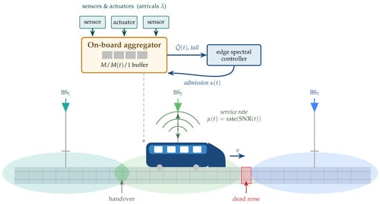
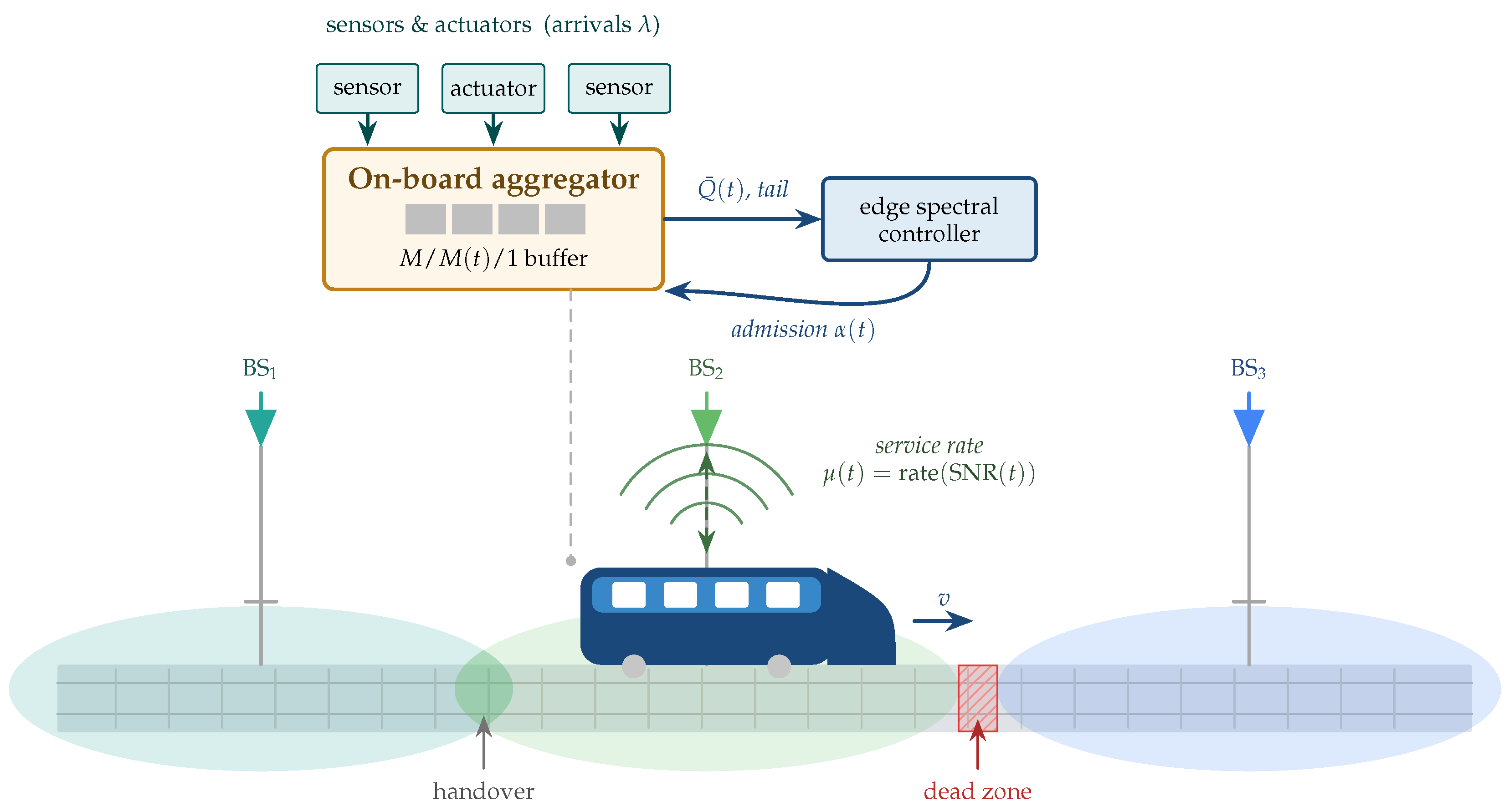
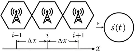
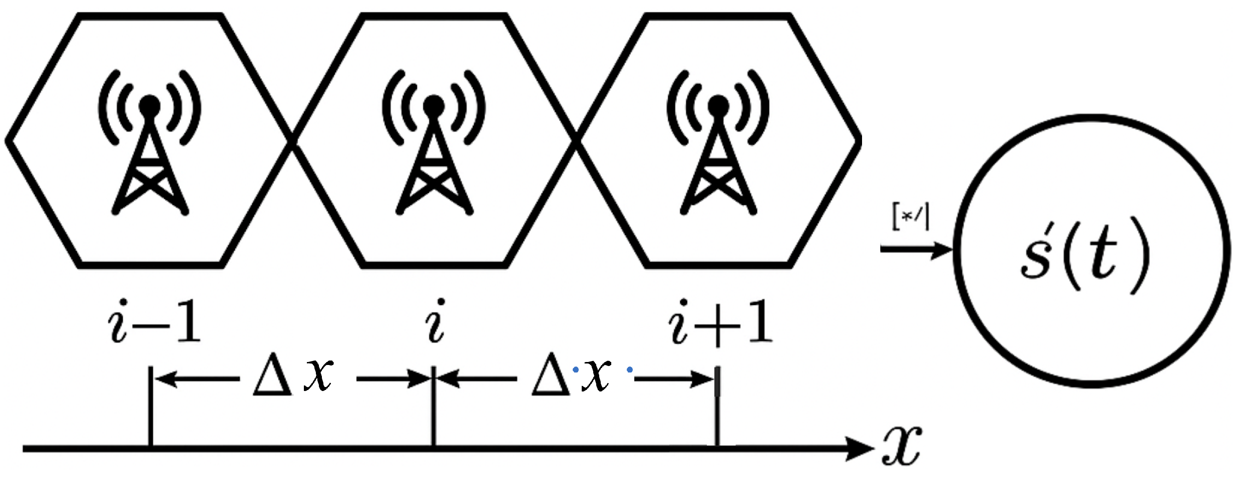
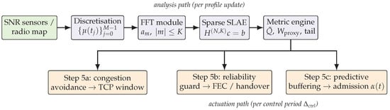
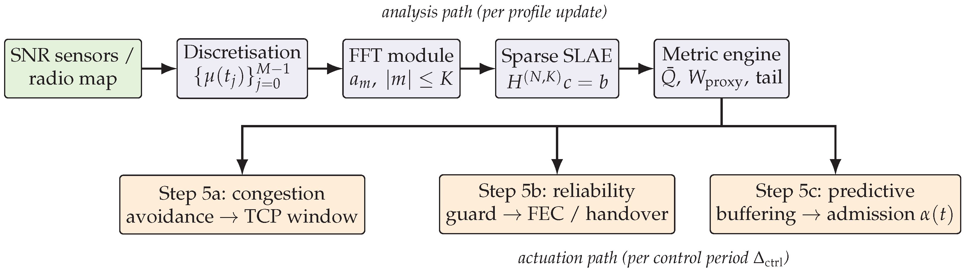
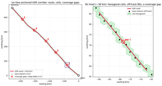
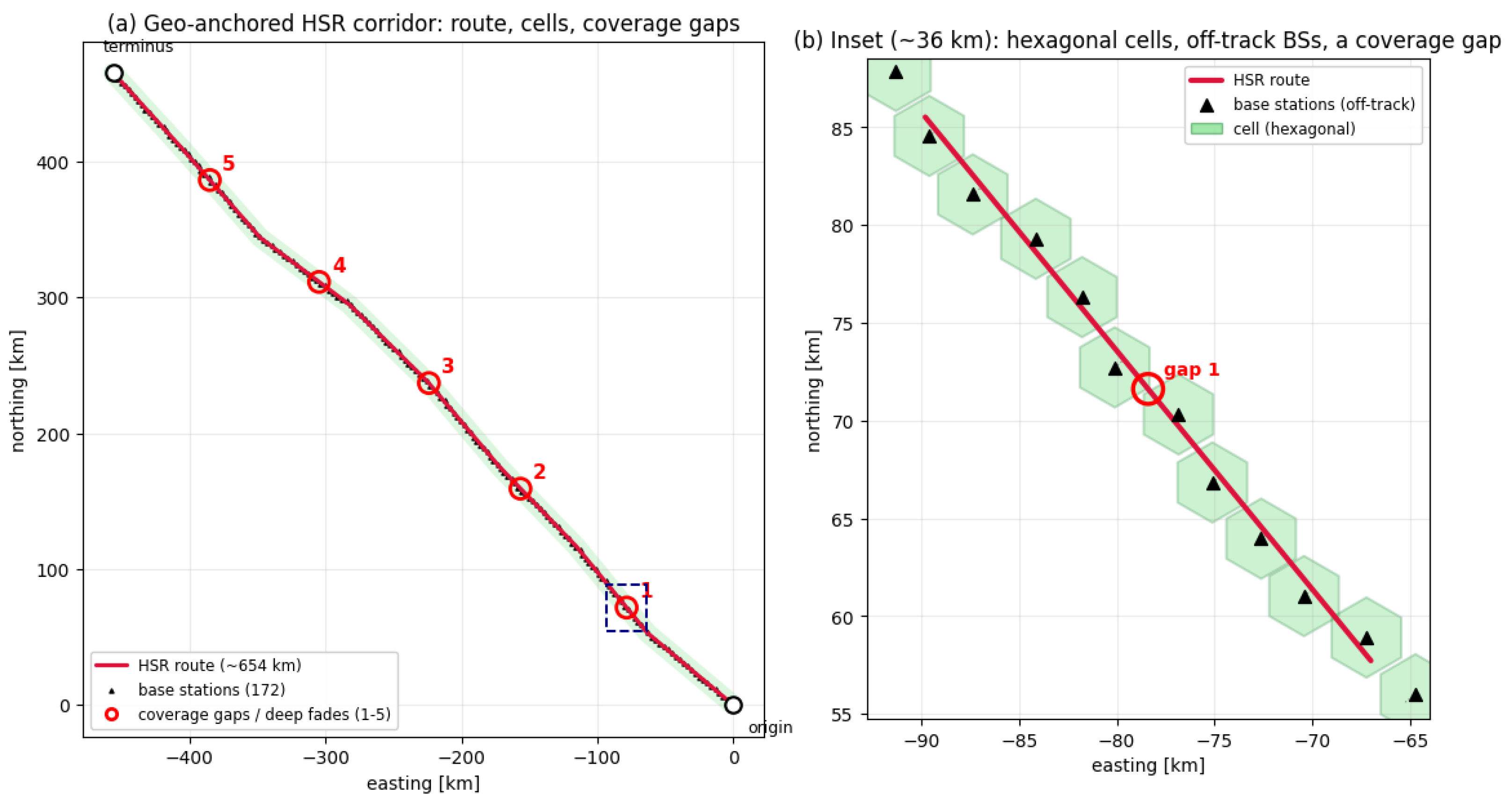
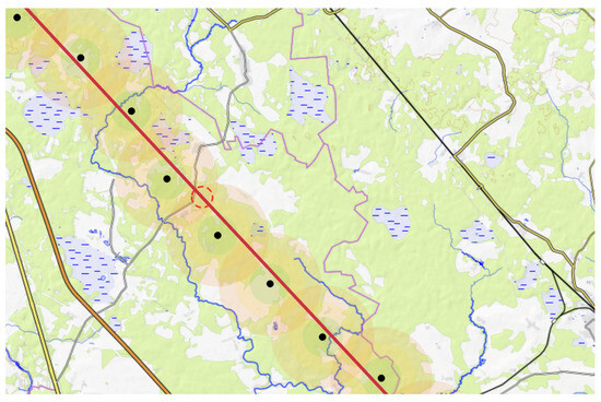
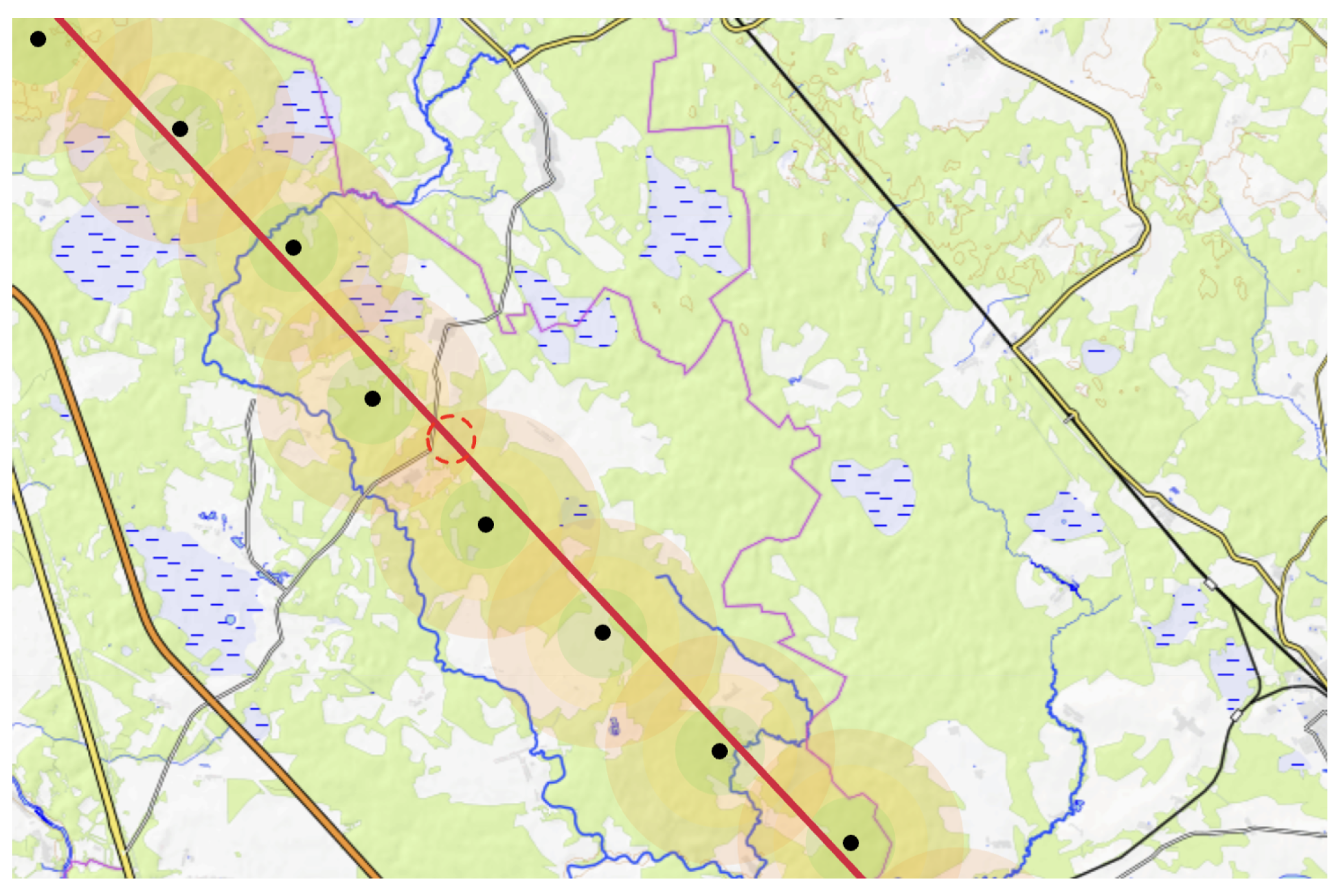
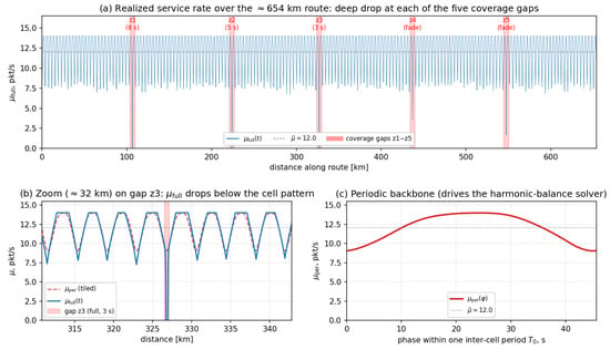
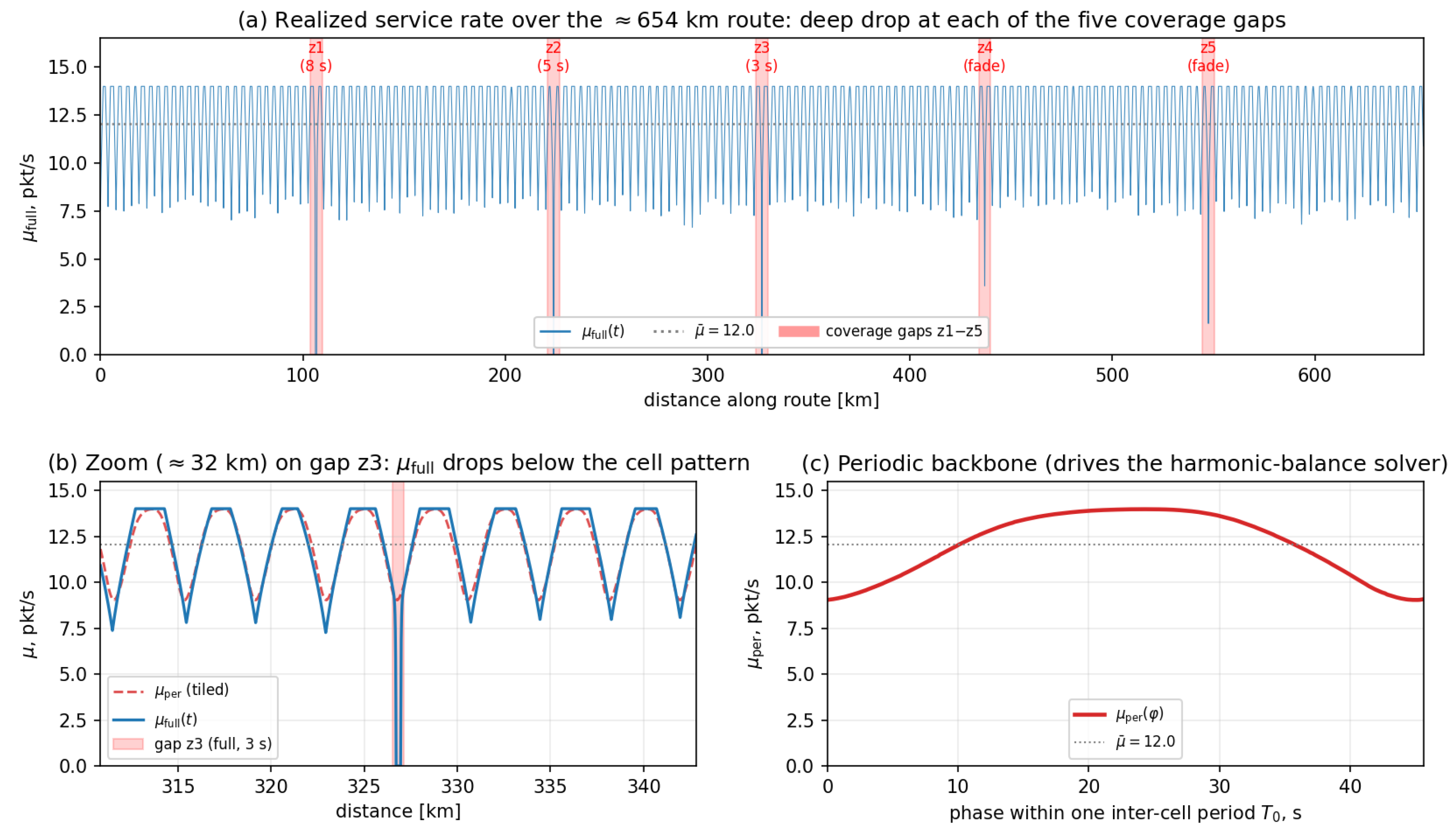
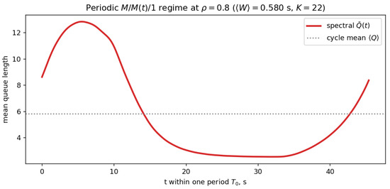
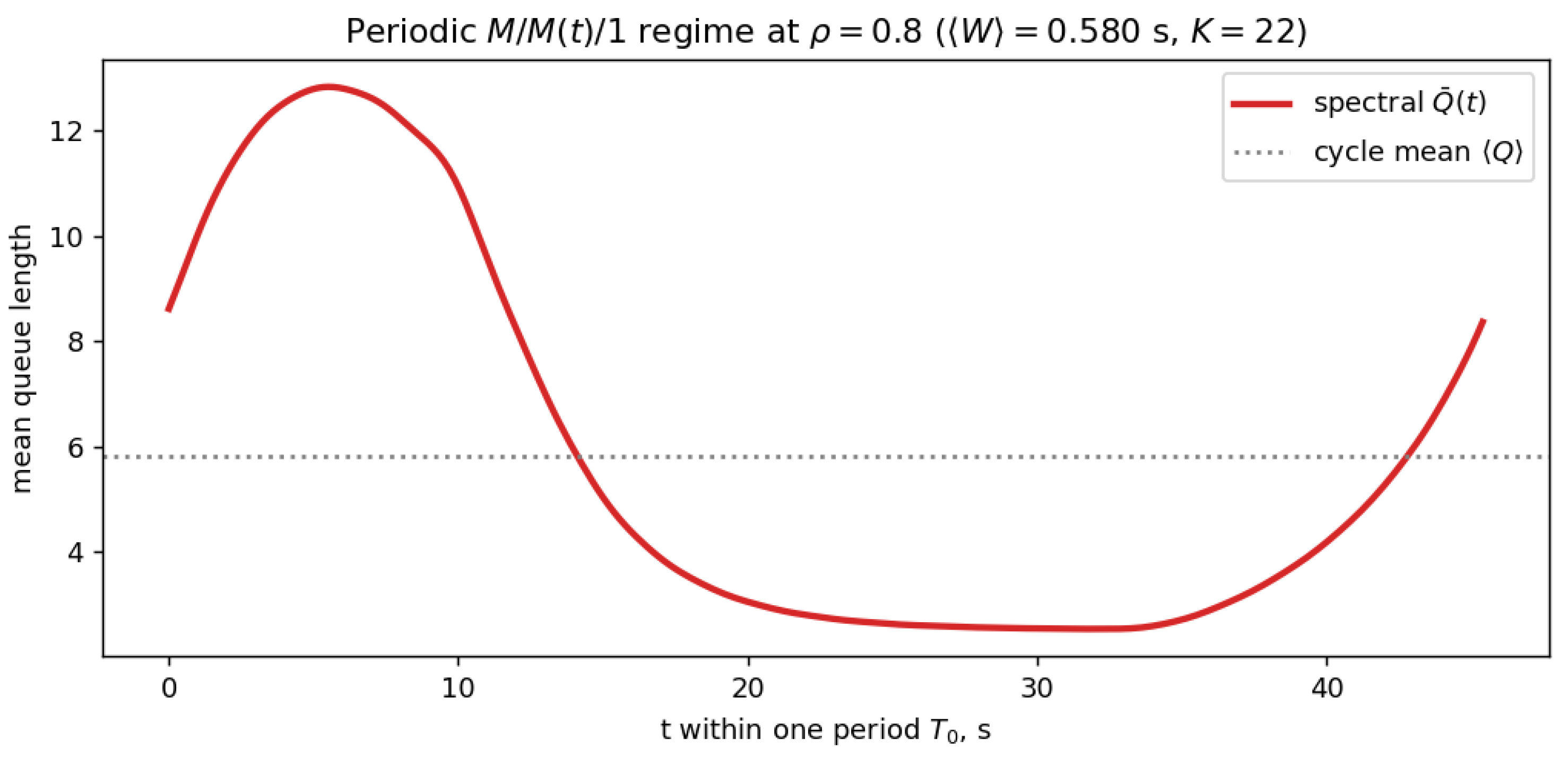
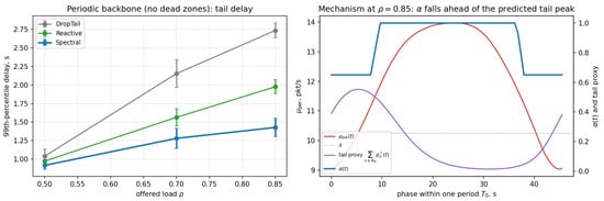
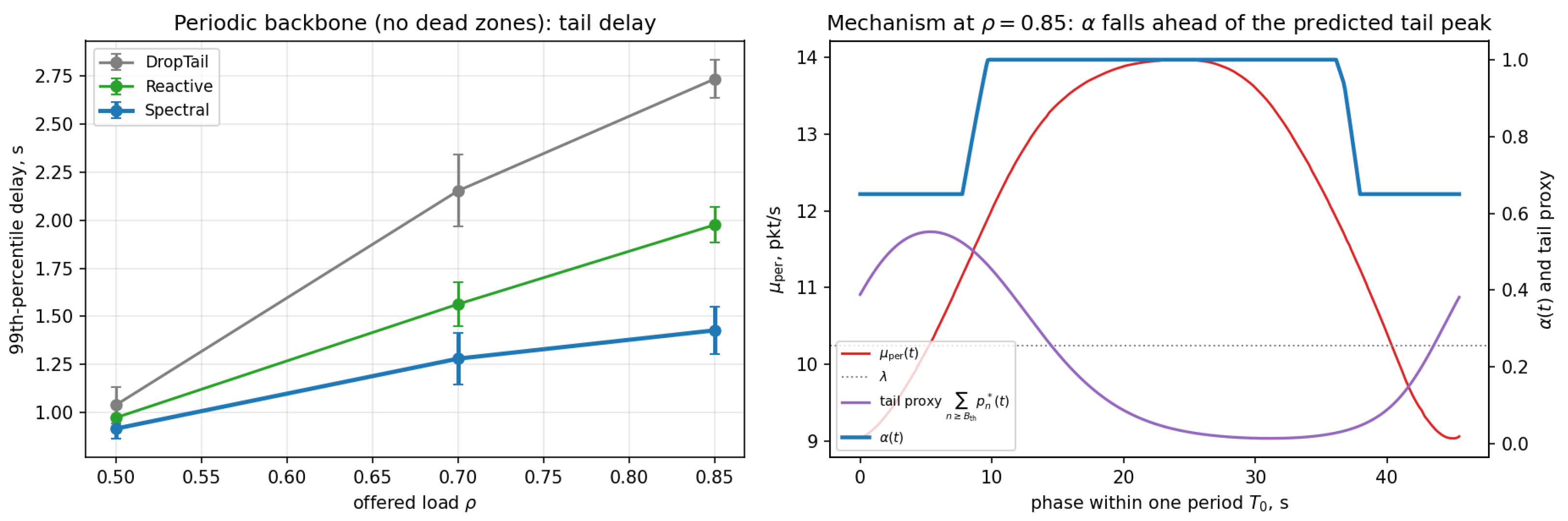
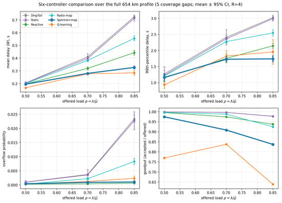
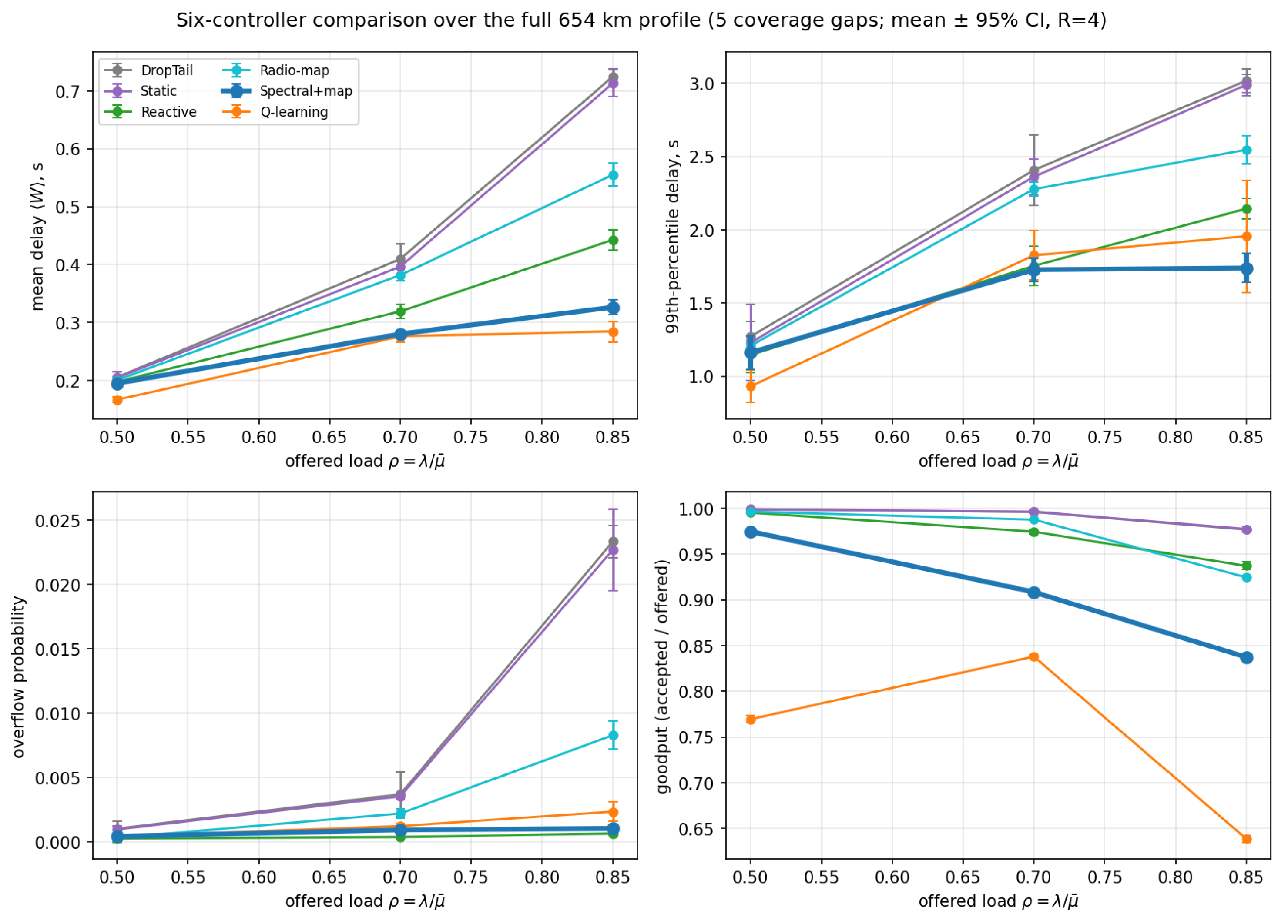
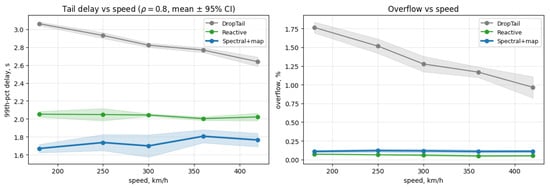
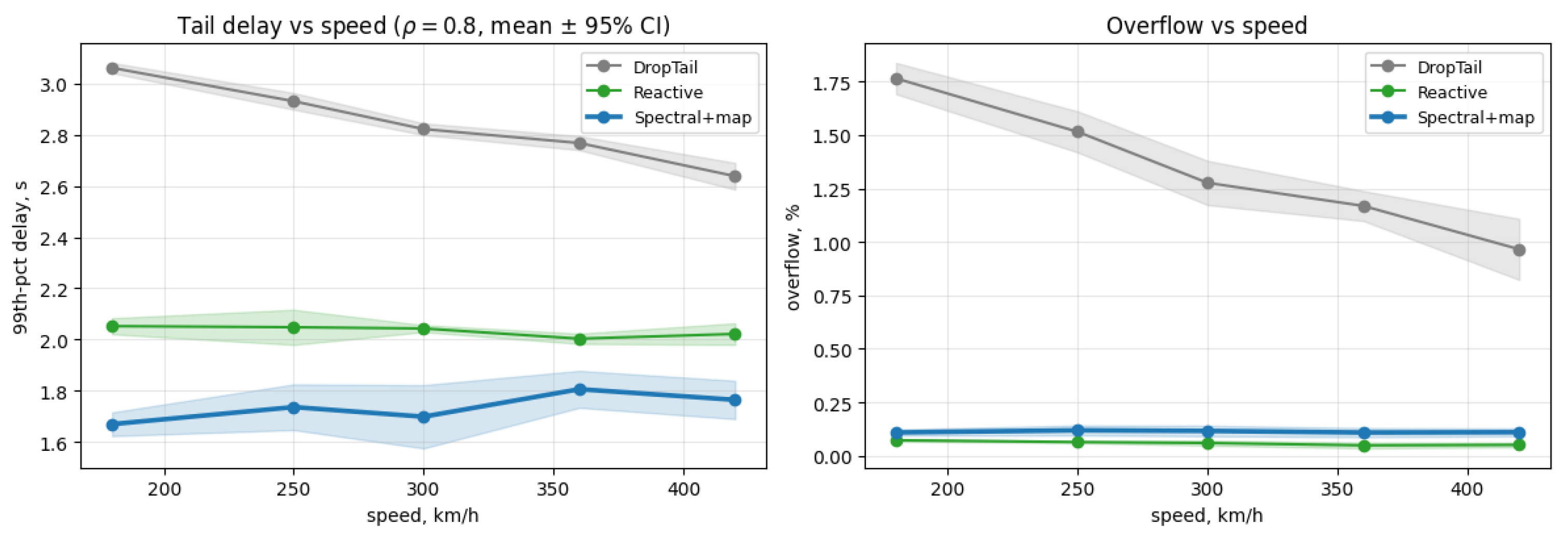
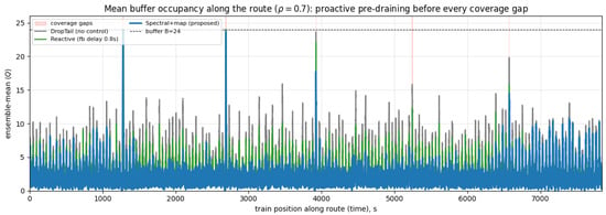
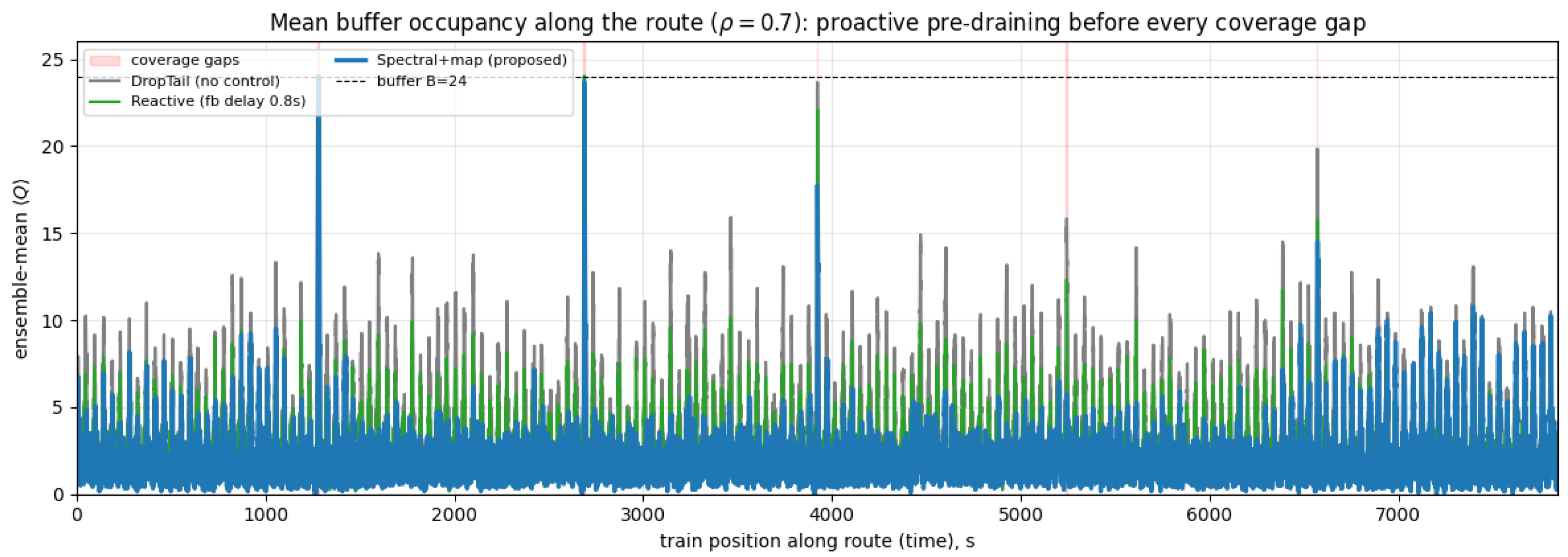
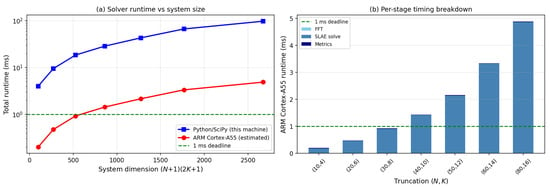
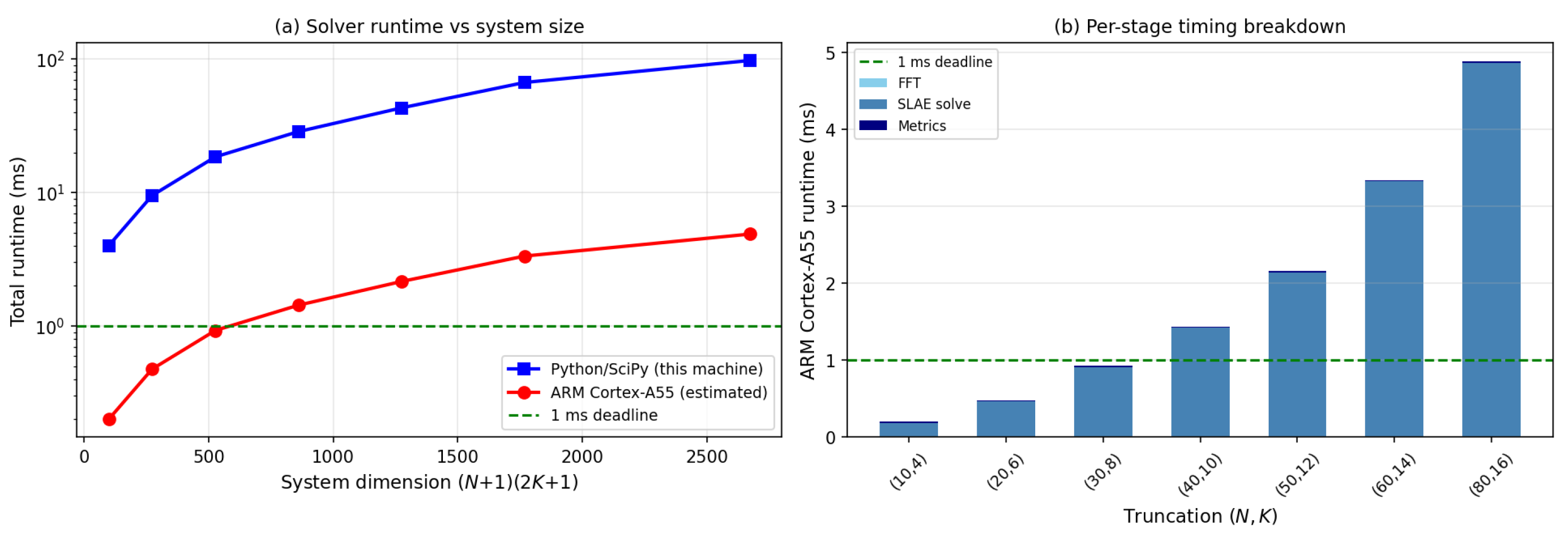

Disclaimer/Publisher’s Note: The statements, opinions and data contained in all publications are solely those of the individual author(s) and contributor(s) and not of MDPI and/or the editor(s). MDPI and/or the editor(s) disclaim responsibility for any injury to people or property resulting from any ideas, methods, instructions or products referred to in the content. |
© 2026 by the authors. Licensee MDPI, Basel, Switzerland. This article is an open access article distributed under the terms and conditions of the Creative Commons Attribution (CC BY) license.