


Abstract
Climate change and rapid urbanisation are intensifying the urban heat island effect, increasing thermal stress, degrading air quality, and leading to rising energy demand. Monitoring neighbourhood-scale heat requires Land Surface Temperature (LST) observations at fine spatial and temporal resolutions, yet satellite thermal products are limited by revisit frequency, acquisition time, and cloud cover. This study developed a novel approach integrating satellite-derived land cover characteristics with continuous contact-based temperature measurements from low-cost LoRaWAN sensors and geostatistical modelling to generate hourly LST maps at 10 m resolution. The technique provides communities with simpler, affordable methods for measuring heat islands and supporting mitigation strategies. Observations from 52 locations across Curtin University’s Bentley campus in Perth, Western Australia, were combined with land cover indices. Empirical Bayesian Kriging captured spatial and temporal urban heat patterns with a root mean square error of approximately 3 °C, representing a bias of near 1 °C. Predictions were consistent with Landsat-derived LST, revealing persistent heat retention over asphalt and cooler conditions associated with vegetation. Integrating satellite-derived predictors with ground measurements provides continuous fine-scale information to identify local heat hotspots and inform targeted mitigation. Unlike satellite data, these low-cost ground measurements could be collected with the help of urban practitioners, developers, and academic institutions.
1. Introduction
Global urban areas have expanded rapidly over the past few decades, primarily driven by population growth, increased economic opportunities and rural-to-urban migration. According to the World Health Organisation [1], approximately 56% of the global population currently lives in urban areas, and this number is projected to rise to around 70% by 2050 [2]. Urbanisation has become one of the defining processes of our time, with profound environmental and societal implications. One of the most critical challenges of urbanisation is the intensification of the Urban Heat Island (UHI) effect, where cities exhibit higher temperatures than their rural surroundings due to the replacement of natural land cover with impervious surfaces such as concrete and asphalt, combined with anthropogenic heat emissions [3]. Intensified UHI exacerbates heat stress, worsens air quality, increases energy demand, and undermines urban resilience to climate change, with disproportionate impacts on vulnerable populations [4]. Consistent temperature measurements are necessary to track potential UHI hotspots in space and time and to develop effective mitigation strategies. In heterogeneous urban environments, this requires observations that resolve thermal variability at fine spatial scales and capture rapid changes throughout the day and night.
In urban climate studies, UHI is traditionally measured using in situ weather data [5]. However, due to advances in satellite technology and thermal remote sensing, UHI is commonly assessed using LST, which gives rise to the concept of Surface Urban Heat Island (SUHI) [6]. SUHI is widely used because LST modulates the near-surface air temperature and reflects the thermal behaviour of urban materials [7]. Over the past few decades, SUHI research has expanded significantly due to advances in thermal remote sensing, in situ monitoring, and numerical modelling approaches. Satellite remote sensing has played a central role in SUHI analysis by providing spatially continuous LST observations over cities. To date, the most widely used thermal infrared (TIR) data have come from the Landsat Thermal Infrared Sensor (TIRS) and the Terra Advanced Spaceborne Thermal Emission and Reflection Radiometer (ASTER) sensors, with moderate spatial resolutions of 60–100 m. However, satellite-derived LST products are constrained by a trade-off between spatial and temporal resolutions [8]. TIR sensors that offer finer spatial detail have infrequent revisit times, while higher-frequency sensors, such as the Moderate Resolution Imaging Spectroradiometer (MODIS) with a spatial resolution of 1000 m, are too coarse for neighbourhood- and street-scale analysis. As such, current satellite products are unable to resolve diurnal and sub-daily SUHI analysis, which are useful for understanding how specific urban surfaces heat and cool, and for monitoring multiday heat events.
To overcome spatial resolution limitations, several LST downscaling approaches have been developed to enhance the spatial resolution of satellite-derived LST. These methods exploit the relationship between LST and higher-resolution surface characteristics derived from Visible and Near-Infrared (VNIR) bands, which are correlated with LST [9]. Commonly used variables are vegetation indices, built-up indices, surface moisture indices, and surface albedo [10,11,12,13,14]. Urban-focused studies have increasingly applied nonlinear regression and Machine Learning (ML) methods to capture the complex relationships between LST and heterogeneous surface composition of urban areas, yielding high-resolution products in selected cases [15,16,17,18]. Recent studies utilised the eXplainable Artificial Intelligence (XAI) techniques, such as Shapley Additive Explanations (SHAP), to interpret the factors contributing to urban LST variations [19,20]. These approaches provide insights into nonlinear relationships among LST and land cover, urban morphology, or anthropogenic indicators, often using models such as random forests or gradient boosting, combined with SHAP-based interpretation [20,21]. However, these studies are typically applied to satellite-derived LST snapshots at the time of thermal sensor acquisition and are therefore constrained by the temporal sampling and clear-sky availability of satellite thermal observations, limiting diurnal SUHI monitoring. To address this limitation, researchers have increasingly explored spatiotemporal fusion techniques that seek to improve temporal resolution while preserving fine spatial detail.
Spatiotemporal fusion methods attempt to improve temporal resolution while maintaining finer spatial detail by combining frequent coarse-resolution observations (e.g., MODIS) with sparse fine-resolution thermal imagery (e.g., Landsat) [22]. The widely used methods include the Spatial and Temporal Adaptive Reflectance Fusion Model (STARFM) approaches and more recent deep learning-based fusion models, such as the Spatiotemporal Temperature Fusion Network (STTFN) [23,24,25,26,27,28]. The result is a synthetic LST dataset characterised by both high spatial and temporal resolutions. However, the accuracy of these models remains dependent on the quality and representativeness of the training data, the temporal alignment of input images, and the computational cost associated with deep learning-based approaches. While effective in certain atmospheric conditions and landscapes, the fusion-based approaches remain constrained by sensor availability and scale mismatches, limiting their capacity for continuous urban monitoring at fine scales.
A recent study by Sara and Rajasekaran [29] have utilised hybrid models combining spatial disaggregation and Diurnal Temperature Cycle (DTC) modelling to reveal fine-scale hotspots during extreme heat events. The investigations demonstrate that high-spatiotemporal LST is essential for identifying localised effects of heatwaves that remain invisible at coarser resolutions. Furthermore, the work of Shahfahad et al. [30] in semi-arid Indian cities, highlights the seasonal dynamics of LST, suggesting that winter thermal patterns are often dominated by surface material emissivity and albedo, whereas summer patterns are governed by proximity to road infrastructure and bare soil indices. This seasonal shift in thermal controls underscores the necessity for models that can adapt to varying radiative regimes throughout the year [30]. Across studies, reported limitations include sensitivity to cloud cover, mismatched acquisition times between sensors, restricted daytime thermal sampling in many datasets, and an effective spatial resolution that often remains too coarse for intra-urban surfaces [31]. These constraints reduce the suitability of purely satellite-based fusion products for continuous diurnal SUHI monitoring at the neighbourhood scale. Given these limitations, complementary observation strategies are required to capture urban thermal variability at finer temporal scales than satellite systems alone can provide.
Terrestrial temperature observations provide direct, high-temporal-resolution measurements, supporting detailed tracking of thermal variability [32]. Traditional station networks often lack spatial density in urban areas and may be located at non-representative sites. Mobile transects can improve spatial detail but are typically limited to selected time windows and require substantial logistical resources [4]. More recently, smart-city and Internet of Things (IoT) deployments have enabled distributed sensor networks to capture intra-urban thermal variability with high temporal frequency [33,34,35]. While these networks can improve temporal continuity, they often remain spatially limited compared with satellite imagery because they measure near-surface air temperature rather than LST [36], complicating direct comparison with SUHI studies. These limitations have encouraged the use of complementary modelling approaches that can better represent urban thermal processes with greater spatial completeness.
In addition, numerical simulations can represent urban thermal processes at very fine spatial and temporal scales by modelling surface energy balance and accounting for urban geometry, materials, and radiative exchange [37]. Such approaches provide valuable insight into diurnal thermal behaviour and the influence of urban morphology [37,38,39]. Still, their performance depends strongly on the availability and quality of high-resolution input data, as well as the parametrisation of surface properties. They also often require substantial computational resources and can be challenging to scale to large urban extents. Collectively, these developments demonstrate that no individual technique fully satisfies the need for continuous, neighbourhood-scale surface temperature information with both high spatial and temporal resolution. This limitation has prompted growing interest in integrating complementary observational approaches that leverage the strengths of different data sources while compensating for their individual shortcomings.
Existing approaches, therefore, address only part of the spatiotemporal resolution challenge. Satellite-derived LST provides spatial continuity but remains limited in temporal frequency and in capturing fine-scale urban surface variability. Conversely, ground-based monitoring provides high temporal resolution and captures local thermal behavior but is typically limited to spatial extent. As such, integrating terrestrial surface temperature measurements with satellite-derived surface characteristics offers a promising pathway to overcome the limitations of either source alone, while also reducing uncertainties associated with atmospheric correction and surface emissivity estimation that affect purely remote sensing-based thermal retrieval in complex urban environments.
Building on this rationale, this study integrates existing satellite-derived surface characteristics with high-frequency, contact-based surface temperature measurements acquired from a low-cost LoRaWAN sensor network with and uncertainty-aware geostatistical interpolation to generate LST maps at high spatial (10 m) and temporal (hourly) resolutions, which has not been done yet in the literature to our knowledge. The framework is evaluated on Curtin University Bentley campus in Perth, Western Australia, for a period of 3 months and assessed using leave-one-out cross-validation and spatial consistency assessment with Landsat-derived LST at satellite overpass times.
2. Materials and Methods
2.1. Study Area
The study was conducted at Curtin University, Bentley campus, and its surrounding areas, located in Perth, Western Australia, covering approximately 400 hectares (Figure 1). The campus is a mixed-use university precinct comprising single and multi-story buildings; extensive managed green open spaces, including lawns and sports fields; significant tree canopy; and planted native vegetation, as well as parking lots and road infrastructure. The precinct also features an expanding area with student accommodation and commercial uses. Its climate is categorised as warm temperate and Mediterranean with wet, cold winters and hot, dry summers, and high temperatures and heatwaves in summertime (from November to April) [40]. Characterised by medium density, the Curtin campus is undergoing active redevelopment, with buildings changing and becoming denser. The study area encompasses various land cover types, which are crucial for assessing UHI variability. The zone surrounding the university campus encompasses major roads, residential blocks, a golf park, and commercial centres.
Figure 1.
Location of the study area (top left), ground-based measurement locations (top right) and a Land Use Land Cover map (bottom) of the study area. Data Sources: Esri basemap, Sentinel-2 imagery and OpenStreetMap for LULC.
2.2. Data
The data for this study comprise ground-based surface temperature measurements collected by sensors connected to a LoRaWAN network, surface-characteristic variables derived from Sentinel-2 (S2) imagery used as temperature predictors, LST derived from Landsat-8 (L8) and Landsat-9 (L9) as a reference for validation, and land cover data.
2.2.1. Ground-Based Temperature Measurements
The surface temperature data are recorded using a network of sensors managed by Curtin Properties under the name “Smart Campus Temperature and Humidity Monitoring” system. It uses LoRaWAN-enabled temperature and humidity sensors to capture environmental data across the Bentley campus. These sensors measure surface temperature by contact at various locations across different land cover types and transmit data via LoRaWAN to the Automatic Weather Station (AWS) IoT core. The recorded data is then integrated into the Smart Campus platform for comprehensive monitoring, analysis, and support of ongoing research on the Curtin campus. We deployed a total of 52 “Dragino LHT65 (sourced from Dragino Technology Co., Shenzhen, China)” sensor nodes, each installed on a sample representative of existing land covers in the area. In this network, the sensors are well distributed across the study area (Figure 1) and continuously used to record temperature data. The surface temperature probe is a resistance temperature detector (RTD) sensor characterised by a contact thermometer packaged in alumina tubes [41]. The LHT65 allows users to transmit data and reach extremely long ranges whilst minimising current consumption. LHT65 features a built-in 2400 mAh battery that lasts over 10 years. The temperature sensors can record temperatures ranging from −55 °C to 125 °C with a resolution of 0.0625 °C. Figure 2A and Figure 2B show, respectively, the LHT65 temperature sensor and a sensor node mounted on a building rooftop in the study area.
Figure 2.
Sensor node: (A) LHT65 temperature sensor; (B) a sensor mounted on a building roof.
The exact location of each sensor probe was recorded in the WGS 1984 UTM zone 50S coordinate system. To minimise scale-representativeness issues, sensor nodes were installed on relatively homogeneous surface patches representative of the dominant land cover types, including asphalt, grass, and roofing materials. This placement minimised edge effects and sub-pixel thermal variability, improving compatibility with the 10 m prediction resolution. Sensors on asphalt and concrete were fixed with thermally conductive epoxy, those on vegetated surfaces were placed on soil beneath the canopy, and roof-mounted sensors were secured with non-invasive adhesive away from edges, vents, and other localised microclimatic influences.
The LHT65 temperature sensors were factory-calibrated by the manufacturer (Dragino) to a stated accuracy of ±0.5 °C across a range of −10 °C to 85 °C [41]. Calibration stability was verified through field intercomparison campaigns conducted at the beginning, midpoint, and end of the monitoring period.
Quality control includes removing duplicate timestamps, transmission-corrupted or incomplete records, physically implausible values, and periods affected by documented installation or contact failures. Subsequent data cleaning and temporal aggregation are described in Section 2.3.1.
The monitoring campaign spans a continuous period from 19 March 2025 to 19 June 2025, covering the autumn-to-early winter transition in Bentley (Perth region), which is characterised by high diurnal variability in surface temperatures. This period offers a wide range of thermal conditions, ranging from warm daytime surfaces to cool nights, allowing evaluation of the model’s robustness under varying heat exchange processes and atmospheric conditions. Moreover, this timeframe coincides with increased cloud cover and intermittent rainfall, conditions under which satellite-derived LST retrievals are often limited. Within this period, the study addresses a critical gap in existing research, as most prior LST downscaling and UHI studies in Perth have examined only summer conditions, where radiative and surface responses are already well documented. The chosen timeframe, therefore, complements these earlier studies while enabling the development and validation of methods that remain reliable under less ideal conditions. Consequently, the model established here can be confidently extrapolated to warmer months, since the same materials and land cover types exhibit consistent thermal behaviour across seasons.
2.2.2. Satellite Data
As this study primarily aims to integrate ground-based temperature observations with satellite-derived data, multispectral imagery from the Multispectral Instrument (MSI) onboard S2 was employed. S2 provides data in the visible, near-infrared (NIR), and shortwave infrared (SWIR) bands at 10 m, offering detailed information on surface characteristics that modulate LST. From these bands, spectral indices were derived and used as temperature predictors. These indices capture biophysical and structural factors that influence thermal variation. Although S2 does not include a TIR band, its high spatial (10 m) and temporal (5 days) resolutions make it well-suited for synergistic applications with thermal sensors and ground observations for supporting urban heat assessment. The S2 product is geometrically and radiometrically calibrated, making it suitable for quantitative surface analysis.
Although S2 imagery is not continuously available due to cloud contamination, the derived spectral indices are not used as temporally dynamic inputs. Instead, they represent spatially explicit surface characteristics that evolve slowly relative to the hourly temperature variations captured by the ground-based sensors. As a result, S2-derived predictors are treated as quasi-static over a five-day window during the study period, reflecting the temporal resolution of S2, and are used to constrain the spatial structure of the LST interpolation rather than to drive temporal variability.
2.2.3. Validation and Spatial Consistency Assessment Data
As independent references for spatial consistency assessment, we utilised L8- and L9-satellite-derived LST, available during the study timeframe. L8 and L9 have two TIR bands with a spatial resolution of 100 m, covering wavelengths from 10.60 to 12.5 μm. Both satellites acquire images of the Earth’s surface over 16 days, with an 8-day offset between their acquisition cycles. The data for L8/L9 are available as Level 2, Tier 1 atmospherically corrected surface reflectance and surface temperature products, with an overpass time between 10:05 and 10:11 AM local time. The LST was downscaled to 10 m using the Geospatial Machine Learning (GeoML) downscaling algorithm by Andriambololonaharisoamalala et al. [42] to a spatial resolution similar to the predicted LST. This choice was informed by our previous evaluation in the same study area during December 2023 and January 2024, in which the GeoML-derived 10 m LST showed higher Pearson’s correlation and lower RMSE against independent ground-based infrared temperature measurements than the original 30 m Landsat LST [42]. Nevertheless, the downscaling introduces an additional source of uncertainty and is therefore considered when interpreting the satellite comparison.
Within the time frame, 11 images from 21 March 2025 to 8 June 2025 were available after cloud cover was analysed and were used for the spatial consistency assessment. Although L8 and L9 each have a nominal 16-day revisit period, the study area is covered by overlapping World Reference System paths. Consequently, combining observations from L8 and L9 and from adjacent paths yields a higher effective temporal sampling than the nominal 8-day repeat interval.
2.2.4. Land Cover Data
Multispectral image classification was conducted using S2 data with the random forest method to obtain land cover classes, including unirrigated grass, grass, asphalt, buildings with roof tiles (hereafter referred to as “roof tiles”), and buildings with Colorbond roofs (hereafter referred to as “Colorbond roof”), which were used for spatial consistency assessment of the predicted LST. The classification results were validated against ground-truth data using Google Earth (GE) imagery, yielding an overall accuracy of 94.88% and a Kappa coefficient of 0.93.
High-resolution GE imagery was used as a qualitative reference to support the interpretation of classification and spatial pattern results, rather than as a quantitative thermal validation source. It provides sub-meter visual information on land cover, surface materials, and urban morphology that cannot be resolved by satellite thermal sensors or ground-based point measurements. GE imagery facilitates visual assessment of whether predicted LST patterns and classified surface features are spatially consistent with observable urban elements, including roads, open spaces, parking areas, vegetation patches, and rooftops. This visual verification supports the interpretation of the spatial realism of the results by confirming alignment between predicted thermal patterns and known surface characteristics.
2.3. Methods
The objective of this study is to generate LST maps at high spatial (10 m) and high temporal (hourly) resolutions to support monitoring of diurnal and nocturnal SUHI dynamics. The workflow integrates high-frequency ground-based contact surface temperature observations with satellite-derived surface predictors and applies geostatistical interpolation to produce continuous hourly LST maps. The overall methodology consists of four sequential steps, as illustrated in Figure 3.
Figure 3.
Schematic workflow for generating 10 m, hourly LST time series maps.
The first step involves data preprocessing, including quality control, data cleaning, and preparation of both ground-based observations and remotely sensed datasets to ensure the reliability and consistency of the input data. The second step focuses on generating temperature predictors from S2 multispectral imagery. These predictors were selected based on their well-established relationships with LST reported in the literature and provide detailed spatial information describing surface characteristics.
The third step applies geostatistical interpolation methods to estimate continuous hourly LST surfaces from ground-based measurements. By incorporating the satellite-derived predictors as auxiliary variables, the interpolation accounts for both the spatial dependence of temperature observations and the influence of land surface characteristics, improving the spatial representation of hourly LST patterns. Due to the limited number of measurement points, geostatistical methods were selected as the primary modelling approaches because they explicitly account for spatial dependence and can provide predictions while characterising associated spatial uncertainty. Specifically, Automatic Universal Kriging (AUK) and Empirical Bayesian Kriging (EBK) were selected for the interpolation analysis [43]. In addition, to assess whether a machine learning approach could provide improved predictive performance under the same limited-sample conditions, a Support Vector Machine (SVM) was used as a benchmark using the same satellite-derived predictors. The comparison, therefore, allows the performance of spatially explicit geostatistical approaches to be evaluated against a machine-learning alternative.
Finally, the predicted hourly LST maps are validated using leave-one-out cross-validation, and the spatial consistency is assessed using Landsat-derived LST data.
2.3.1. Data Pre-Processing
Data pre-processing was conducted for both ground-based temperature observations and satellite-derived datasets to ensure consistency and accuracy. The workflow included outlier removal, temporal aggregation, and filtering for cloud contamination. For the ground-based LST data, initial cleaning involved removing incomplete or erroneous records. This step aimed to ensure that missing timestamps, duplicated records, and unrealistic temperature values (e.g., negative temperatures recorded during midday) are deleted, which can result from temporary sensor malfunctions or transmission losses. The data were then aggregated to an hourly temporal resolution to standardise the temporal scale across different monitoring sites and to reduce high-frequency noise. For the satellite-derived data, S2 cloud-free scenes over the study area have been selected.
No temporal gap-filling or data assimilation of S2 imagery was performed, as the S2-derived predictors are not required at hourly temporal resolution. The hourly LST time series is generated independently of S2 temporal availability, relying instead on continuous ground-based measurements, with S2 providing only spatially static constraints.
2.3.2. Temperature Predictors
High-spatial-resolution S2 multispectral data were used to compute temperature predictors for the two kriging interpolation methods. The predictors were chosen based on their established physical relationships with LST and their widespread application in thermal remote sensing studies. First, surface albedo has been widely recognised as an important predictor of spatial variations in LST. Albedo governs the proportion of incoming solar radiation reflected by the Earth’s surface, thereby influencing the surface energy balance and the amount of energy available for heating [44,45]. Second, the Normalised Difference Vegetation Index (NDVI) provides a measure of vegetation density and vigour. Vegetation moderates surface temperatures through shading and evapotranspiration, resulting in a strong and well-established inverse relationship between the NDVI and LST [46,47]. Third, the Normalised Difference Built-up Index (NDBI) characterises the spatial distribution and intensity of built-up areas. Urban materials such as concrete and asphalt generally exhibit greater heat storage capacity and lower evapotranspiration than vegetated surfaces, making the NDBI a reliable indicator of elevated LST in urban environments [48,49]. Lastly, the Normalised Difference Water Index (NDWI) has been commonly used as an indicator of moisture-related thermal variability and has demonstrated strong relationships with LST across a range of land cover types. Moisture availability influences latent heat flux through evaporation and evapotranspiration, which reduces surface temperatures [50,51]. Together, these variables describe complementary radiative, vegetative, built-up, and moisture controls on LST and therefore provide physically meaningful covariates for temperature interpolation.
All predictors are shown in Table 1, including their equations where B, G, R, NIR, SWIR1, and SWIR2 denote the blue, green, red, near-infrared, shortwave infrared 1, and shortwave infrared 2 bands, respectively. The script indicates the reflectance value of each band.
Table 1.
Temperature predictors.
To ensure that variables with meaningful relationships to LST were included in the interpolation models, correlation analysis was conducted to examine relationships among the satellite-derived predictor variables and to reduce redundancy. Pearson correlation coefficients were computed to identify highly correlated predictors. Variables exhibiting strong collinearity were evaluated to avoid instability in the interpolation models and to ensure that each predictor contributed distinct spatial information. This analysis supported the research objective by ensuring that predictor selection was physically meaningful and statistically robust, thereby improving the reliability of the subsequent geostatistical interpolation.
2.3.3. Geostatistical Interpolation and Machine Learning Benchmark
Geostatistical spatial interpolation is a popular technique that predicts missing data values from surrounding measured locations. In kriging, the predicted value at an unsampled location is estimated as a weighted linear combination of existing nearby observations given in Equation (1):
where is the estimated value, is the known measurements, and is the kriging weights determined by minimising the estimation variance under the unbiasedness constraint. The spatial dependence among the sampled points is modelled by the semivariogram, defined in Equation (2) in accordance with [52]:
A semivariogram quantifies the similarity between observations separated by distance h. The weights assigned to the sample points depend on the distances to the prediction point. For this study, two types of interpolation methods were used to predict LST, Automatic Universal Kriging (AUK) and Empirical Bayesian Kriging (EBK), were used as the primary approaches for predicting surface temperature. In addition, Support Vector Machine (SVM) with a radial basis function kernel was evaluated as a machine learning benchmark to assess whether a nonlinear predictor-based model could provide improved predictive performance with the available 52 sensor observations. AUK and EBK were selected as the primary geostatistical approaches because they explicitly model spatial autocorrelation and provide prediction uncertainty, which are important characteristics for spatially heterogeneous urban surface-temperature fields. In contrast, SVM can capture nonlinear relationships between observed surface temperature and predictor variables but does not explicitly model spatial dependence. Its inclusion, therefore, provides a complementary point of comparison with the spatially explicit geostatistical approaches.
AUK and EBK provide the best linear unbiased predictions and associated prediction variances while modelling spatial autocorrelation through the variogram. AUK automates variogram fitting, reducing the subjectivity associated with manually selecting variogram parameters, and provides a computationally efficient and reproducible benchmark. However, AUK treats the fitted variogram as known, which can lead to the underestimation of prediction uncertainty. EBK addresses this limitation by estimating multiple variogram models through Bayesian simulation and thereby accounting for uncertainty in the variogram parameters. This is particularly beneficial in heterogeneous urban environments, where variogram estimation can be challenging given limited sample sizes. Its main disadvantage is higher computational demand, particularly for large spatiotemporal datasets. For the present application, EBK was expected to provide an improved representation of uncertainty in the presence of strong spatial heterogeneity, while AUK was expected to provide a computationally efficient geostatistical comparison.
Because urban surface temperature exhibits strong spatial heterogeneity, individual point measurements cannot be assumed to directly represent the thermal state of a complete 10 m pixel. The point-based observations were therefore treated as spatial samples of the underlying temperature field rather than as pixel-scale observations. The geostatistical models estimate continuous surface-temperature fields by explicitly accounting for spatial dependence and local variability among nearby observations. The SVM benchmark, in contrast, estimates temperature from the nonlinear relationship between observed temperatures and satellite-derived predictor variables, without explicitly modelling spatial autocorrelation. This comparison was used to determine whether the additional representation of spatial dependence provided by the geostatistical approaches resulted in improved predictive performance for the present dataset.
Automatic Universal Kriging (AUK)
A key challenge in geostatistical interpolation is specifying and fitting the variogram model, which strongly influences the accuracy of kriging predictions. The variogram model is a function of semi-variance versus distance that provides a fit to the sample variogram [53]. Fitting a variogram model involves selecting the model type, such as spherical and Gaussian, and the associated parameters (e.g., nugget, sill, range), which are often determined through a subjective visual comparison of the variogram model and the sample variogram [54]. For this study, we utilise the automatic variogram fitting process developed by [53] and implemented in the R package “Automap” developed by Hiemstra [55].
With AUK, it is assumed that the temperature measurements from the network is a realisation of a spatial random field , described by the linear model in Equation (3) [56]:
where are the trend coefficients, and are unknown, is the ith known predictor at location , is a zero-mean, second-order stationary process with covariance defined by the fitted variogram. The best linear unbiased prediction for the grid node is given in Equation (4) [53]:
where are the estimated regression coefficients, are the observations, is the design matrix, , is the variance-covariance matrix of , and is a vector containing the covariance between the residuals of prediction and observations, and the vector is the best linear estimator of , given by Equation (5):
More details about automatic kriging can be seen in the article by Hiemstra et al. [53].
Empirical Bayesian Kriging (EBK)
EBK is an advanced geostatistical interpolation method that explicitly incorporates uncertainty in variogram estimation into the prediction process [57]. While AUK assumes that the fitted variogram fully captures the spatial structure, EBK recognises that variogram parameters are estimated from limited samples and are therefore uncertain. This uncertainty can propagate into kriging predictions, potentially underestimating prediction error if ignored [58]. This approach provides both predicted LST surfaces and more realistic prediction standard errors, improving reliability in heterogeneous urban landscapes or regions with irregular sensor coverage. The robust uncertainty quantification of EBK makes it particularly suitable for high-spatial-resolution LST modelling. EBK was implemented in ArcGIS Pro 3.6 Geostatistical Analysis of ESRI [59].
EBK repeatedly simulates multiple semivariogram models from prior distributions and updates them using observed data through Bayesian updating. The EBK predictor at an unknown location is expressed in Equation (6) in accordance with Gribov and Krivoruchko [58]:
with the associated variance shown in Equation (7):
where denotes the temperature at the location , is the vector of observed temperatures from sensor nodes, is the number of variogram simulations, represents the set of semivariogram parameters for the ith simulation, and are the conditional expectation and variance of the kriging prediction given , and is the Bayesian weight of each model, given in Equation (8):
Support Vector Machine (SVM) Benchmark
To assess whether a machine learning approach could improve predictive performance given the limited number of spatial observations available in this study, SVR with a Radial Basis Function (RBF) kernel was implemented as an additional benchmark. The model used the same four S2-derived predictors as the geostatistical models, namely surface albedo, the NDVI, the NDWI, and the NDBI, with the ground-based surface temperature measurements as the response variable. The SVM hyperparameters were the cost parameter (C), the RBF kernel parameter (γ), and the epsilon-insensitive loss parameter (ɛ). C controls the penalty assigned to prediction errors, γ controls the spatial locality of the nonlinear response in predictor space, and ɛ defines the width of the insensitive loss region around the predicted values.
During model tuning, a nested cross-validation procedure was adopted. For each outer leave-one-out iteration, one observation was withheld as an independent test observation, while the remaining observations were used for model training and hyperparameter optimisation. Within each outer training set, 5-fold cross-validation was used to identify the optimal combination of C, γ, and ɛ. The SVM was then fitted to the complete outer training set using the selected hyperparameters and used to predict the withheld observation. This process was repeated for all observations at each timestamp.
2.3.4. Validation and Spatial Consistency Assessment Methods
Two evaluation methods were used to assess the performance of the proposed approach in generating high spatiotemporal-resolution LST maps. First, cross-validation was employed to evaluate the predictive performance and internal consistency of the two models (EBK and AUK) using a leave-one-out sample. Second, the spatial consistency of the predicted LST was evaluated using satellite-derived LST. It is important to mention that these two evaluation steps serve different purposes. Cross-validation assesses how well the interpolation models reproduce observed contact-based surface temperature measurements at unsampled locations. In contrast, the comparison with satellite-derived LST is not intended as a physical validation of the ground-based sensor measurements, but rather as an independent assessment of the spatial consistency of the predicted LST relative to established thermal infrared satellite products.
Cross-Validation
To independently validate the predictive performance and uncertainty quantification of the model, we performed a “Leave-One-Out” cross-validation, as described by Pebesma [54]. This validation method enables the determination of how well the interpolation model fits the data. It works by removing a single point from the dataset and using all remaining points to predict the location of the removed point [60]. Therefore, each data point is sequentially removed and its value is predicted using a model trained on the remaining n − 1 observations. The predicted value is then compared to the measured value using the Root Mean Square Error (RMSE), bias, and the coefficient of determination (R2) as assessment metrics, respectively, given in Equations (13)–(15) [60]:
where is the number of observations, is the observed temperature at the location , is the predicted value at from the model trained without this point, and is the mean of observed values. For this method, the predicted value was then compared to the observed LST.
The RMSE quantifies the average magnitude of the difference between predicted and measured values. It represents how far, on average, model predictions deviate from the actual observations. Lower RMSE indicates better predictive performance. The bias measures the systematic error of a mode, whether predictions tend to be consistently higher or lower than the observed values. A bias close to 0 indicates that the predictions are unbiased on average; a positive bias suggests the model overestimates the observations; and a negative bias suggests the model underestimates them. R2 provide a measure of how well the predicted values explain the variability of the observed values. A value close to 1 indicates good predictive performance.
Because this validation relies exclusively on the ground-based sensor network, it directly assesses the interpolation framework’s internal reliability under varying thermal conditions throughout the day. R2 indicates how well spatial or spatiotemporal predictors capture the pattern and variability of temperature, while RMSE and bias quantify the absolute prediction errors.
Independent Spatial Consistency Assessment with Satellite-Derived LST
An independent evaluation of the predicted LST fields was conducted using LST derived from L8 and L9 data acquired at approximately 10:04–10:11 local time. The satellite-derived LST was downscaled to 10 m to match the spatial resolution of the predicted LST maps [42]. The 10 m resolution supports a scale-consistent comparison, reduces spatial aggregation bias associated with the coarser Landsat thermal data, and better represents temperature variability across heterogeneous urban surfaces. This comparison aims to assess the degree to which the predicted LST reproduces the spatial patterns and relative thermal contrasts observed in satellite-derived LST at the time of satellite overpass. Because contact-based surface temperature measurements and radiometric LST represent different physical quantities, this evaluation is explicitly interpreted as a spatial consistency assessment, rather than absolute physical validation. Instead, the comparison is used to examine whether the predicted LST reproduces the relative thermal patterns observed by satellite thermal infrared data at overpass time. This interpretation recognises the differences in measurement principle, spatial support, emissivity effects, and mixed-pixel behaviour while still providing a useful reference for evaluating the spatial realism of the predicted maps.
For each Landsat acquisition, the corresponding hourly aggregated LHT65 surface-temperature value at 10:00 AM local time was used. The Landsat–LHT65 temporal differences were between 4 and 11 min across the 11 validation dates. No temporal interpolation was applied to the satellite observations, and each Landsat LST-derived data was compared with the 10:00 AM ground-based measurements for the corresponding acquisition date.
The agreement between the two datasets was quantified using Pearson’s correlation coefficient r, which provides the degree of correlation between the two datasets as computed in Equation (16) after [61]. This metric was computed for the entire study area and separately for land cover classes to examine class-dependent behaviour. By combining cross-validation with ground-based observations and an independent assessment of spatial consistency using satellite-derived LST, the evaluation framework provides a robust and transparent evaluation of both model accuracy and spatial realism.
Any remaining discrepancies between predicted and satellite-derived LST may partly reflect limitations in scale representativeness, particularly in areas with strong sub-pixel heterogeneity or mixed land cover. All comparisons with satellite-derived LST were performed using only the available Landsat acquisitions at their respective overpass times, without temporal interpolation or temporal aggregation across scenes. Equation (16) is defined as follows:
where is the total number of observations, is the ith observation or reference data, is the mean value of , is the corresponding predicted LST data, and is the mean value of .
The value of r ranges from −1 to 1. Values close to 1 indicate a strong positive linear association, meaning that predicted values increase consistently with observed values, while values near 0 indicate little or no linear relationship. Pearson’s correlation coefficient, therefore, evaluates the strength of the relationship between the predicted and Landsat-derived LSTs.
3. Results and Evaluation
3.1. High-Spatiotemporal Resolution LST
Using the proposed framework, a fine-scale LST time series dataset was generated for the study area at 10 m spatial resolution and an hourly temporal resolution, producing 2218 hourly LST maps during the monitoring period. The resulting dataset provides a spatially continuous representation of surface temperature patterns while capturing diurnal variability and sub-daily scales. These LST maps were generated using AUK and EBK predictive modelling with the NDVI, the NDBI, the NDWI, and surface albedo as temperature predictors. The incorporation of these variables enabled the interpolation models to account for heterogeneity in land cover and surface energy balance, thus improving the spatial representation of LST across different urban environments.
Figure 4 and Figure 5 show examples of the predicted LST maps produced by EBK and AUK, respectively. These representative maps illustrate the spatial patterns of LST for three distinct times of day: morning, afternoon, and evening on 20 March 2025, providing a comparative view of the diurnal temperature variations captured by each interpolation approach. These examples highlight temporal variability in LST in relation to the underlying surface characteristics, including strong daytime heating and evening cooling. They also show the persistent warmth of surfaces covered by asphalt throughout the day and the rapid cooling of vegetated areas after sunset.
Figure 4.
Predicted LST using EBK interpolation on 20 March 2025, showing diurnal progression: (A) morning (6:00 am) with minimal solar heating, (B) afternoon peak (2:00 pm) showing maximum thermal contrast between built and vegetated surfaces, and (C) evening (9:00 pm) illustrating differential cooling rates across land cover types. Colour scale ranges from 10 °C to 56 °C to capture the full diurnal range.
Figure 5.
Predicted LST using AUK interpolation on 20 March 2025: (A) morning, (B) afternoon peak, and (C) evening. Colour scale depicted as defined in Figure 4. Visual comparison suggests spatial patterns similar to those of LST produced with EBK, but quantitative evaluation reveals differences in accuracy (Section 3.2).
The results suggested that the land cover types have a significant impact on LST patterns. The thermal contrast between these land cover types is evident in Figure 4 and Figure 5, with built areas consistently warmer (red and orange hues) than vegetated surfaces (green and blue hues). These spatial contrasts establish that the predicted LSTs capture the expected urban thermal behaviour and provide a basis for subsequent quantitative evaluation and class-based interpretation.
Diurnal variations also showed systematically cooler conditions in the morning than in the evening, consistent with heat storage and delayed heat release in urban materials. These figures also indicate that vegetated areas, such as parks, tend to be cooler during the daytime due to evapotranspiration, with the strongest cooling effect occurring in the afternoon when the thermal contrast with surrounding built-up surfaces is most pronounced. Visual inspection suggests no pronounced differences between the outputs of the EBK and AUK models, particularly during the afternoon. However, the evaluation presented in Section 3.1 reveals statistically clear differences between the two approaches.
3.2. Validation of the Predicted LST
The validation results are interpreted not only in terms of numerical performance metrics but also considering the physical processes governing urban surface temperatures, measurement-scale effects, and differences across observation modalities. This interpretation is essential for understanding the conditions under which the proposed framework performs best and where uncertainties remain.
The predicted LST maps generated using the AUK and EBK approaches were evaluated using leave-one-out cross-validation and spatial consistency check with Landsat-derived LST.
3.2.1. Cross-Validation of the Predicted LST
As presented in Table 2, the cross-validation results quantify the predictive accuracy of the AUK, EBK, and benchmark SVM models. The reported metrics, including the root mean square error (RMSE), bias, and coefficient of determination (R2), evaluate how well each model predicts temperature values at unsampled locations using observed data. These results also enable a direct comparison between the two kriging approaches, revealing their respective performance in representing the spatial variability of LST across the study area.
Table 2.
Error RMSE, bias, and coefficient of determination (R2)—result of cross-validation for the AUK, EBK, and SVM models.
Table 2 presents the cross-validation performance of EBK, AUK, and SVM models for the overall dataset and for the morning, afternoon, and evening periods. Across all models, the RMSE values range from 1.627 °C to 6.088 °C, with the lowest error observed for EBK during the evening (1.627 °C) and the highest for SVM in the afternoon (6.088 °C). Bias values were generally low, ranging from 0.010 °C to 1.139 °C, indicating a small systematic deviation between the predicted and observed surface temperatures. The coefficient of determination (R2) ranges from 0.579 to 0.952. Overall, EBK achieved the strongest predictive performance, with an RMSE of 2.975 °C and an R2 of 0.903, compared with 3.625 °C and 0.881 for AUK and 3.740 °C and 0.768 for SVM, respectively. Although SVM exhibited the lowest overall bias (0.072 °C), its lower R2 indicates weaker predictive power for the observed spatial variability.
A consistent temporal pattern was observed across the models, with prediction errors generally increasing during the afternoon and decreasing toward the evening. The afternoon represented the most challenging period, with RMSE values of 4.504 °C for EBK, 5.871 °C for AUK, and 6.088 °C for SVM, and corresponding R2 values of 0.803, 0.772, and 0.579, respectively. The comparatively larger errors during the afternoon are likely associated with stronger solar forcing and greater thermal contrasts between built-up and vegetated surfaces, which increase local spatial heterogeneity. In contrast, evening conditions produced lower errors and higher R2 values, particularly for EBK (RMSE = 1.627 °C; R2 = 0.952), indicating more spatially coherent cooling patterns.
Overall, EBK provided the strongest predictive performance among the three approaches, achieving the lowest RMSE and highest R2 for the overall dataset and for each period of the day. AUK generally showed intermediate performance, while SVM exhibited relatively low bias but weaker reproduction of the observed spatial variability. The stronger performance of EBK is consistent with its ability to account for uncertainty in variogram estimation and spatial heterogeneity through Bayesian simulation. These results indicate that, for the present sensor density and predictor set, explicitly modelling spatial dependence provided an advantage over the machine learning SVM benchmark.
3.2.2. Assessment of the Predicted LST with Satellite-Derived Data
The validation of the predicted LST from the EBK and AUK models was also conducted against LST derived from L8 and L9 data at the time of satellite overpass. Landsat acquisitions occurred between approximately 10:04 AM and 10:11 AM local time, while the corresponding ground-based comparison used the hourly aggregated LHT65 surface-temperature value at 10:00 AM. The resulting temporal difference between the satellite acquisition and the ground-based value therefore ranged from 4 to 11 min across the 11 validation dates. This relatively short temporal offset should nevertheless be considered because urban surface temperatures can change rapidly during daytime heating. The assessment metrics presented in Table 3 are based on the Pearson correlation coefficient (r).
Table 3.
Pearson’s correlation coefficient (r) between satellite-derived LST and the predicted LST with AUK and EBK at Landsat overpass times, including the temporal difference between the satellite acquisition and the 10:00 AM LHT65 observation.
As presented in Table 3, the EBK and AUK models demonstrate good overall agreement with satellite-derived LST across the different dates, with EBK exhibiting a wider but generally stronger range of correlations from 0.161 to 0.835 than AUK, where the correlation coefficients range from 0.447 to 0.751. The highest correlations for both methods occur on 21 March 2025 (hereafter, all other dates are given without the year, referring to 2025) (0.835 for EBK, 0.751 for AUK). In contrast, the weakest correlations are observed for EBK on 24 May (0.161) and for AUK on 8 June (0.447). Notably, correlations decline from March to June, indicating reduced rank-order agreement later in the season, even as EBK typically maintains smaller absolute errors. Taken together, both methods reproduce the spatial pattern of LST around the overpass time, but EBK provides more reasonable and comparatively stable predictions. In contrast, AUK occasionally yields a slightly higher correlation on specific days (e.g., 29 April, 16 May, 24 May, 8 June) at the cost of larger errors.
3.2.3. Interpretation of Validation Results
The validation results reveal systematic variations in model performance across time of day, land cover classes, and validation datasets, which can be explained by underlying physical and methodological factors.
First, prediction errors were consistently higher in the afternoon than in the morning or evening across all three models. This pattern is likely associated with stronger shortwave radiative forcing during peak solar hours, which amplifies thermal contrasts among adjacent surfaces, including sunlit and shaded areas, buildings, asphalt, and vegetation. These strong spatial gradients increase local thermal heterogeneity and make the spatial prediction problem more challenging, even when land-cover-based predictors are incorporated. In contrast, evening and nighttime conditions are increasingly influenced by heat storage and release, which generally produce more spatially coherent cooling patterns. This is reflected in the substantially lower evening RMSE and higher R2, particularly for EBK.
Second, the model comparison indicates that EBK generally provided the strongest predictive performance across the different periods of the day. For the overall dataset, EBK achieved an RMSE of 2.976 °C and an R2 of 0.903, compared with 3.625 °C and 0.881 for AUK and 3.740 °C and 0.768 for SVM. Although SVM produced relatively low bias, its lower R2 indicates weaker reproduction of the observed variability. The difference was particularly pronounced during the afternoon, when SVM achieved an RMSE of 6.088 °C and an R2 of 0.579, whereas EBK achieved 4.504 °C and 0.803. These results suggest that, for the present sensor density and predictor set, explicitly modelling spatial dependence provided an advantage over the nonlinear predictor-based SVM benchmark.
Third, the land-cover-specific assessment indicates that surfaces with relatively homogeneous thermal properties, such as asphalt and unirrigated grass, generally exhibited stronger spatial correspondence with satellite-derived LST than highly heterogeneous or radiatively complex surfaces. Colorbond roofs showed weaker correspondence, which may be associated with variations in roof colour, reflectance, emissivity, and roof geometry. These characteristics can produce substantial sub-pixel thermal variability and are difficult to represent fully using land-cover classification alone. The lower correlations observed for this class should therefore be interpreted in the context of both surface heterogeneity and differences in measurement scale.
Fourth, differences between the predicted surface temperature and the satellite-derived LST arise in part from fundamental differences in measurement principles. The ground-based sensors measure contact-based surface temperature at discrete locations, whereas Landsat estimates radiometric land surface temperature over its instantaneous field of view and is influenced by emissivity, atmospheric correction, and mixed-pixel effects. Consequently, the satellite comparison should be interpreted primarily as an assessment of spatial consistency and relative thermal patterns rather than as a direct measure of absolute physical accuracy. Differences in magnitude between the two datasets, therefore, do not necessarily represent prediction error alone.
Finally, the gradual decline in spatial correlation from March to June may reflect increasing atmospheric variability, cloud contamination, and seasonal changes in surface moisture and vegetation conditions. These factors can affect both the thermal state of the surface and the quality and representativeness of satellite-derived LST, thereby reducing agreement in the spatial ranking of relatively warmer and cooler surfaces.
Together, these findings indicate that the observed validation patterns reflect interactions among urban surface physics, spatial heterogeneity, observation scale, and measurement modality, rather than random model behaviour. The results highlight both the strengths and limitations of the proposed framework, particularly under strongly heterogeneous daytime conditions and for thermally complex surface types.
While urban LST exhibits significant spatial heterogeneity that challenges strict stationarity assumptions, EBK was specifically designed to accommodate such non-stationarity through Bayesian simulation of multiple semivariogram models. This approach provides robust predictions without requiring residuals to be strictly stationary, as the Bayesian framework explicitly accounts for uncertainty in the variogram arising from spatial heterogeneity. Given the limited sample size (n = 52), additional diagnostic tests such as Moran’s I correlogram would be underpowered and potentially misleading. Our cross-validation results, which demonstrate strong predictive performance (R2 = 0.903, RMSE = 2.98 °C for EBK), provide empirical evidence that the EBK framework effectively captures urban LST variability despite potential violations of strict stationarity.
3.3. Land-Cover-Specific Diurnal Behaviour and Spatial Consistency Assessment of EBK
The thermal pattern mentioned above is quantified in Figure 6, which illustrates the diurnal variation in LST across five representative land cover classes (unirrigated grass, grass, asphalt, Colorbond roofs, and roof tiles) of the study area for a seven-day extract period within the study timeframe. EBK predictions were used for this analysis because the validation results identified EBK as the best-performing interpolation model. At approximately 2:00 pm, the thermal gradient indicates that surfaces covered by asphalt have the highest LST, followed by Colorbond roofs, unirrigated grass, roof tiles, and grass (the lowest temperature). Figure 7 focuses on a single day (22 March 2025) to illustrate the detailed diurnal variations, highlighting the heating and cooling rate differences among land cover classes. During the midnight to early morning period, the order of elevated surface temperatures shifts slightly, with asphalt maintaining the highest LST, followed by grass, unirrigated grass, Colorbond roof, and roof tiles. This suggests that vegetated areas, particularly unirrigated grass, retain less heat overnight than impervious surfaces, whereas asphalt consistently exhibits a strong heat storage capacity.
Figure 6.
Temporal profile of land cover classes from 23 March to 29 March 2025, derived from EBK-predicted LST time series maps.
Figure 7.
Diurnal variation in surface temperature of various land covers in the study area on 22 March 2025, generated from EBK-predicted LST time series maps.
In the morning, Colorbond roofs exhibit a rapid temperature increase, surpassing that of asphalt, and reading their peak surface temperatures around midday (12:00 pm). After this peak, Colorbond roof temperatures begin to decline, while asphalt continues to accumulate heat throughout the afternoon. Asphalt surfaces cool more slowly than other land cover types and remain the warmest until midnight, highlighting their dominant role in sustaining elevated nocturnal surface temperatures. These class-specific profiles demonstrate that the hourly time series supports analysis of both daytime heating and nocturnal heat retention, which is central to the stated monitoring objective.
3.4. Land-Cover-Specific Spatial Consistency Assessment with EBK
Based on the aggregate spatial consistency check against satellite-derived LST, we conducted a stratified, land-cover-specific comparison in which the EBK-predicted LST, the best-performing model from the preceding analysis, was evaluated against L8/L9 satellite-derived LST across the five land cover classes. Table 4 presents the Pearson correlation coefficient between the two datasets for the five classes.
Table 4.
Pearson’s correlation coefficient (r) between predicted LST with the EBK model and satellite-derived LST for land cover classes on different dates.
Across land cover classes, as shown in Table 4, the agreement between LST predicted by the EBK model and satellite-derived LST clearly depends on class type and acquisition date. Averaged over dates, unirrigated grass exhibits the strongest correspondence (mean r = 0.57), followed by asphalt (mean r = 0.54). Roof tiles show intermediate performance (mean r = 0.50), whereas grass is weaker on average (mean r = 0.37). Colorbond roofs are consistently the most challenging class (mean r = 0.23), with a low peak of 0.418 and a minimum of 0.103.
The colour variation in the Colorbond roof class, as shown in a sample area in Figure 8, is highly heterogeneous, and the different colours affect LST; therefore, this land cover class shows lower correlation with Landsat LST. Colorbond is a brand of pre-painted steel roofing material widely used in Australia, available in multiple colours. The thermal behaviour of these roofs can be influenced by colour-dependent albedo (dark coloured Colorbond absorbs more solar radiation and reaches higher temperature than light colours), low thermal mass (steel roofs have low thermal mass, causing rapid heating and cooling in response to changing solar radiation), emissivity effects (metal surfaces have low and variable emissivity, which complicate LST retrieval), and view angle effects (anisotropic thermal emission from metal surfaces can cause directional brightness temperature variations).
Figure 8.
Colour variations in the Colorbond roof class. This image is a sample of the study area extracted from Google Earth imagery.
In contrast, the colours of other classes are more homogeneous and do not significantly impact the correlation. Considering dates across all classes, late March, especially 29 March, achieves the highest overall agreement (mean across classes of 0.62), while 24 May is uniformly poor (mean around 0.22), with minima for asphalt, roof tiles, and unirrigated grass. The pattern suggests that surfaces with more homogeneous thermal behaviour (asphalt, unirrigated grass) tend to have high correlation, whereas highly reflective, low-emissivity metal roofing (Colorbond) and phenologically dynamic vegetation (grass) reduce correlation, likely due to class-specific emissivity and moisture dynamics. The seasonal degradation from March to June is consistent with increased atmospheric and meteorological variability during these periods, particularly as indicated by the data captured on 15 and 24 May, containing abundant cloud cover. When examining the overall correlation values, the 10 m spatial resolution of the TIR image used as a reference should be considered, as highly heterogeneous urban areas are affected by mixed pixels.
4. Discussion and Conclusions
This study developed an integrated approach to generating high-spatial- and temporal-resolution LST maps by combining ground-based measurements, satellite-derived surface predictors, and geostatistical interpolation. A distinctive feature of the study is its ability to produce hourly LST maps at 10 m resolution, supporting the monitoring of both daytime heating and nocturnal cooling patterns across heterogeneous urban surfaces. This addresses a key limitation of satellite-derived LST products, which are often constrained by revisit frequency, cloud cover, and acquisition time. The approach is particularly relevant for urban environments where surface characteristics vary strongly over short distances [62].
The results demonstrate that the predicted LST maps capture clear thermal contrasts among land cover types. These patterns are consistent with existing UHI mapping studies [4,63] and reinforce the established role of land covers in controlling urban thermal variability [15,42,64]. The findings further confirm that vegetation indices, built-up indices, surface albedo, and moisture indicators provide meaningful spatial predictors of LST. The NDVI reflects vegetation cooling through evapotranspiration and shading [65,66,67], the NDBI represents the thermal influence of impervious surfaces [48,68], surface albedo indicates differences in shortwave radiation absorption [69], and the NDWI captures moisture-related cooling effects [70].
Methodologically, comparing AUK and EBK against the additional nested SVM benchmark highlights the value of uncertainty-aware geostatistical modelling for fine-scale urban temperature prediction. EBK generally outperformed both AUK and SVM, particularly during periods of strong spatial thermal variability, because it accounts for uncertainty in variogram estimation through a Bayesian framework. This makes EBK well-suited to heterogeneous urban areas where sensor coverage is uneven, and surface temperatures vary sharply over short distances. Although the S2-derived predictors improved the spatial representation of surface characteristics, they mainly constrained spatial contrasts rather than driving hourly temporal variation. SVM produced relatively low bias, but its overall RMSE and R2 were inferior to those of the geostatistical approaches, especially during the afternoon, when contrasts between built and vegetated surfaces and between sunlit and shaded areas increased local thermal heterogeneity. These findings suggest that, for the present sensor density and predictor set, explicitly accounting for spatial dependence provides an advantage over relying solely on nonlinear relationships between temperature and satellite-derived surface characteristics. However, this should not be interpreted as evidence that SVM is generally unsuitable for small datasets; rather, it indicates that EBK was more appropriate under the specific spatial and thermal conditions investigated here.
An additional contribution of this study is the complementary use of ground-based and satellite-derived observations. Contact-based surface temperature measurements and satellite-derived LST represent physically related but distinct quantities. The observed differences between predicted LST and Landsat-derived LST should therefore be interpreted as differences between measurement modalities rather than simple errors. Ground sensors measure local contact-based surface temperature, whereas satellite products estimate radiometric skin temperature over a pixel. Another difference is the temporal mismatch between satellite acquisitions and ground-based measurements. In this study, the Landsat overpasses occurred 4 to 11 min after the hourly aggregated LHT65 value assigned to 10:00 AM. Although this difference is relatively small, rapid surface heating during the morning may produce measurable temperature changes over such an interval, particularly over thermally contrasting urban materials. The observed differences between the predicted and satellite-derived temperature fields should therefore be interpreted in the context of both temporal mismatch and the distinct measurement principles and spatial supports of the two datasets. Despite these differences, the correlations between the predicted and satellite-derived LSTs indicate that both datasets capture similar spatial thermal structures. This supports the use of ground-based sensor networks to complement satellite observations, especially for continuous monitoring between satellite overpasses.
The low-cost nature of the sensor network makes this approach accessible to a wide range of stakeholders, including community groups, local governments, schools, and academic institutions. By deploying sensors across residential neighbourhoods, schools, and public spaces, communities could generate localised thermal data, build public awareness of urban heat risks, and contribute directly to evidence-based decision-making. This participatory monitoring model, akin to citizen science initiatives in other environmental domains, could substantially extend the spatial coverage and societal impact of urban heat studies.
The capacity to generate hourly LST maps at 10 m resolution has practical implications for urban heat management. Fine-scale thermal maps can identify persistent hotspots such as asphalt parking areas, exposed roofs, and unirrigated grass, helping communities and planners prioritise mitigation measures such as tree planting, shade structures, irrigation, and the replacement of heat-retaining materials. The hourly resolution is also important because it shows when specific surfaces reach peak temperatures and when they retain heat into the evening.
Although this study measured surface temperature rather than air temperature, LST remains important because hot surfaces influence the thermal environment experienced by pedestrians through longwave radiation [71]. Therefore, the resulting LST maps can support heat exposure assessment when combined with pedestrian activity, land use, or population data. In addition, dense ground-based sensor networks could complement official weather stations by providing localised thermal information in urban areas where people live, work, and move.
Several limitations should be acknowledged for this study. First, prediction quality depends on the density and spatial distribution of sensors. Although the 52-sensor network captured major land cover types across the study area, areas far from sensors or characterised by strong micro-scale heterogeneity may still have higher uncertainty. This also limits the spatial density available for interpolation and constrained additional analyses, such as residual spatial autocorrelation testing and land-cover-specific validation. Second, the 10 m spatial resolution, while finer than many satellite LST products, may not fully capture sub-metre thermal variability such as narrow shaded zones, small impervious patches, or within-roof material differences. Point-based measurements may therefore not always represent the full thermal variability within a 10 m pixel.
Third, S2-derived predictors are temporally sparse and cannot fully represent short-term changes in surface conditions, such as rainfall-driven moisture changes or rapid vegetation responses. In this study, hourly temporal variability was mainly driven by ground-based measurements, while S2 inputs provided spatial constraints. Fourth, the present approach relies primarily on two-dimensional land cover information and does not explicitly account for 3D urban morphology, such as building height, street canyon geometry, shading, or sky view factor, all of which can influence urban thermal patterns. A further limitation concerns the spatial–statistical assumptions underlying kriging-based interpolation. Urban surface temperature fields are strongly heterogeneous, and residual spatial structures may vary across land cover types and distance classes.
Future research should test the approach in larger, more diverse urban environments to evaluate its transferability across different climates, urban forms, and land cover compositions. While our study focused on asphalt as a representative impervious surface, given its prevalence in urban environments, alternative surfaces such as gravel, permeable pavers, and grasscrete also offer potential heat mitigation benefits. Gravel parking areas, for instance, may exhibit lower surface temperatures than asphalt due to increased albedo and reduced thermal mass, although they present challenges for surface marking and accessibility. Future investigation should systematically compare the thermal performance of different pavement materials across a wider range of surface types, including gravel, porous asphalt, and grasscrete, to provide urban planners with a comprehensive evidence base for material selection. Involving urban planners, developers, and landscape architects in sensor deployment and data interpretation could facilitate the translation of research findings into practice, while citizen science initiatives could extend monitoring to under-sampled areas.
In terms of methodology, further work should also investigate optimal sensor placement strategies and the minimum sensor density required to maintain reliable prediction accuracy at the city scale. In addition, the next study should deploy a denser and more balanced sensor network to enable robust residual spatial autocorrelation testing, such as Moran’s I correlograms, and land-cover-specific cross-validation across heterogeneous urban surfaces. Moreover, incorporating 3D urban morphology from LiDAR or digital surface models would help improve the representation of shading and urban geometry effects. Finally, additional air temperature sensors installed at standard pedestrian height could support the development of heat exposure metrics more directly linked to public health, while UAV thermal surveys could help characterise sub-pixel temperature variability and improve interpretation of 10 m predictions.
Overall, the study demonstrates that combining high-frequency ground-based measurements with satellite-derived surface characteristics can provide continuous, fine-scale information on urban surface heat dynamics. The resulting LST maps can support the identification of persistent heat hotspots and inform targeted heat-mitigation strategies, such as shading, greening, cool roofing and other surface material interventions. Future work should test the approach in other urban and climatic settings, expand sensor coverage, incorporate urban morphology variables, and collect coincident radiometric ground measurements to further improve model transferability and cross-sensor interpretation. Ultimately, this novel integration of satellite data with low-cost ground sensors offers a pathway for engaging academics, professionals, and citizens in collaborative efforts to address urban heat and build climate-resilient communities.
Author Contributions
Conceptualization, Ratovoson Robert Andriambololonaharisoamalala, Petra Helmholz, Ivana Ivánová, Dimitri Bulatov and Eriita Jones; methodology, Ratovoson Robert Andriambololonaharisoamalala, Dimitri Bulatov, Ivana Ivánová, Yongze Song and Eriita Jones; Software, Ratovoson Robert Andriambololonaharisoamalala, Petra Helmholz, Dimitri Bulatov, Ivana Ivánová and Yongze Song; validation, Ratovoson Robert Andriambololonaharisoamalala, Petra Helmholz, Ivana Ivánová, Yongze Song, Susannah Soon and Eriita Jones; formal analysis, Ratovoson Robert Andriambololonaharisoamalala, Petra Helmholz, Dimitri Bulatov, Ivana Ivánová, Susannah Soon and Eriita Jones; investigation, Ratovoson Robert Andriambololonaharisoamalala, Petra Helmholz, and Ivana Ivánová; resources, Ratovoson Robert Andriambololonaharisoamalala, Petra Helmholz, Ivana Ivánová and Dimitri Bulatov; data curation, Ratovoson Robert Andriambololonaharisoamalala, Dimitri Bulatov and Yongze Song; writing—original draft, Ratovoson Robert Andriambololonaharisoamalala and Petra Helmholz; writing—review and editing, Ratovoson Robert Andriambololonaharisoamalala, Petra Helmholz, Dimitri Bulatov, Ivana Ivánová, Yongze Song, Susannah Soon and Eriita Jones; visualization, Ratovoson Robert Andriambololonaharisoamalala, Ivana Ivánová, Dimitri Bulatov, Yongze Song and Susannah Soon; supervision, Petra Helmholz, Ivana Ivánová., Eriita Jones, Susannah Soon, and Dimitri Bulatov; project administration, Ratovoson Robert Andriambololonaharisoamalala, Ivana Ivánová and Petra Helmholz; funding acquisition, Ratovoson Robert Andriambololonaharisoamalala, Petra Helmholz and Ivana Ivánová All authors have read and agreed to the published version of the manuscript.
Funding
This work has been supported by the SmartSat CRC, whose activities are funded by the Australian Government’s CRC Program.
Data Availability Statement
The data that support the findings of this study are available from the corresponding author upon reasonable request.
Acknowledgments
The authors would like to express their gratitude to colleagues at Curtin Properties for their invaluable contributions to the deployment of the sensor network. They also gratefully acknowledge Eva Strauss for her insightful comments, which significantly improved this manuscript.
Conflicts of Interest
The authors declare no conflicts of interest.
Abbreviations
The following abbreviations are used in this manuscript:
| UHI | Urban heat island |
| LST | Land surface temperature |
| SUHI | Surface urban heat island |
| B | Blue |
| G | Green |
| R | Red |
| NIR | Near-infrared |
| VNIR | Visible and near-infrared |
| SWIR | Shortwave infrared |
| TIR | Thermal infrared |
| TIRS | Thermal infrared sensor |
| L8 | Landsat-8 |
| L9 | Landsat-9 |
| S2 | Sentinel-2 |
| ASTER | Advanced Spaceborne Thermal Emission and Reflection Radiometer |
| MODIS | Moderate-resolution Imaging Spectroradiometer |
| TM | Thematic Mapper |
| ETM+ | Enhanced Thematic Mapper Plus |
| MSI | Multispectral Imager |
| GeoML | Geospatial Machine Learning |
| STARFM | Spatial and Temporal Adaptive Reflectance Fusion Model |
| ESTARFM | Enhanced Spatial and Temporal Adaptive Reflectance Fusion Model |
| STTFN | Spatiotemporal Temperature Fusion Network |
| LoRaWAN | Long Range Wide Area Network |
| AWS | Automatic Weather Station |
| LHT | LoRaWAN Humidity and Temperature |
| mAh | milliampere-hour |
| UTM | Universal Transverse Mercator |
| WGS | World Geodetic System |
| AUK | Automatic universal kriging |
| EBK | Empirical Bayesian kriging |
| NDVI | Normalised difference vegetation index |
| NDBI | Normalised difference built-up index |
| NDWI | Normalised difference water index |
References
- World Health Organisation. Heat and Health; World Health Organisation: Geneva, Switzerland, 2020. [Google Scholar]
- Ritchie, H.; Samborska, V.; Roser, M. Urbanization. 2018. Available online: https://ourworldindata.org/urbanization (accessed on 2 February 2026).
- Team, O.E.H. How Cities Can Beat Extreme Heat|OGC Study on Urban Heat Mapping. 2025. Available online: https://www.ogc.org/blog-article/how-cities-can-beat-extreme-heat-mapping-the-invisible-killer/ (accessed on 20 November 2025).
- Shandas, V.; Voelkel, J.; Williams, J.; Hoffman, J. Integrating Satellite and Ground Measurements for Predicting Locations of Extreme Urban Heat. Climate 2019, 7, 5. [Google Scholar] [CrossRef] [Scilit]
- Howard, L. The Climate of London: Deduced from Meteorological Observations Made in the Metropolis and at Various Places Around it; Harvey and Darton, J. and A. Arch, Longman, Hatchard, S. Highley and R. Hunter: London, UK, 1833; Volume 3. [Google Scholar]
- Mills, G.; Futcher, J.; Stewart, I.D. The Urban Heat Island: Its Energetic Basis and Management. In Urban Microclimate Modelling for Comfort and Energy Studies; Palme, M., Salvati, A., Eds.; Springer International Publishing: Cham, Switzerland, 2021; pp. 23–53. [Google Scholar]
- Hulley, G.; Shivers, S.; Wetherley, E.; Cudd, R. New ECOSTRESS and MODIS Land Surface Temperature Data Reveal Fine-Scale Heat Vulnerability in Cities: A Case Study for Los Angeles County, California. Remote Sens. 2019, 11, 2136. [Google Scholar] [CrossRef] [Scilit]
- Andriambololonaharisoamalala, R.; Helmholz, P.; Ivánová, I.; Jones, E.; Soon, S.; Bulatov, D.; Song, Y. Enhancing the spatial and temporal resolution of satellite-derived land surface temperature in urban environments: A systematic literature review. Urban Clim. 2025, 60, 102345. [Google Scholar] [CrossRef] [Scilit]
- Pang, B.; Yue, J.; Zhao, G.; Xu, Z. Statistical Downscaling of Temperature with the Random Forest Model. Adv. Meteorol. 2017, 2017, 7265178. [Google Scholar] [CrossRef] [Scilit]
- Choe, Y.J.; Yom, J.H. Improving accuracy of land surface temperature prediction model based on deep-learning. Spat. Inf. Res. 2020, 28, 377–382. [Google Scholar] [CrossRef] [Scilit]
- Ebrahimy, H.; Azadbakht, M. Downscaling MODIS land surface temperature over a heterogeneous area: An investigation of machine learning techniques, feature selection, and impacts of mixed pixels. Comput. Geosci. 2019, 124, 93–102. [Google Scholar] [CrossRef] [Scilit]
- Zawadzka, J.; Corstanje, R.; Harris, J.; Truckell, I. Downscaling Landsat-8 land surface temperature maps in diverse urban landscapes using multivariate adaptive regression splines and very high resolution auxiliary data. Int. J. Digit. Earth 2020, 13, 899–914. [Google Scholar] [CrossRef] [Scilit]
- Lezama Valdes, L.-M.; Katurji, M.; Meyer, H. A Machine Learning Based Downscaling Approach to Produce High Spatio-Temporal Resolution Land Surface Temperature of the Antarctic Dry Valleys from MODIS Data. Remote Sens. 2021, 13, 4673. [Google Scholar] [CrossRef] [Scilit]
- Liang, L.; Li, J.; Chen, Y.H.; Xia, H.P.; Chen, Q. An Auto-Adjusted Kernel Method for Thermal Sharpening With Local and Object-Based Window Strategies. IEEE J. Sel. Top. Appl. Earth Obs. Remote Sens. 2021, 14, 3659–3668. [Google Scholar] [CrossRef] [Scilit]
- Dominguez, A.; Kleissl, J.; Luvall, J.C.; Rickman, D.L. High-resolution urban thermal sharpener (HUTS). Remote Sens. Environ. 2011, 115, 1772–1780. [Google Scholar] [CrossRef] [Scilit]
- Bechtel, B.; Zaksek, K.; Hoshyaripour, G. Downscaling Land Surface Temperature in an Urban Area: A Case Study for Hamburg, Germany. Remote Sens. 2012, 4, 3184–3200. [Google Scholar] [CrossRef] [Scilit]
- Gao, F.; Kustas, W.P.; Anderson, M.C. A Data Mining Approach for Sharpening Thermal Satellite Imagery over Land. Remote Sens. 2012, 4, 3287–3319. [Google Scholar] [CrossRef] [Scilit]
- Feng, X.; Foody, G.; Aplin, P.; Gosling, S.N. Enhancing the spatial resolution of satellite-derived land surface temperature mapping for urban areas. Sustain. Cities Soc. 2015, 19, 341–348. [Google Scholar] [CrossRef] [Scilit]
- Zhang, P.; Zhang, J.; Liu, Z.; Liu, Y.; Chen, Z. Relationship between land surface temperature and air quality in urban and suburban areas: Dynamic changes and interaction effects. Sustain. Cities Soc. 2025, 118, 106043. [Google Scholar] [CrossRef] [Scilit]
- Sheng, T.; Zhang, Z.; Qian, Z.; Ma, P.; Xie, W.; Zeng, Y.; Zhang, K.; Sun, Z.; Yu, J.; Chen, M. Examining urban agglomeration heat island with explainable AI: An enhanced consideration of anthropogenic heat emissions. Urban Clim. 2025, 59, 102251. [Google Scholar] [CrossRef] [Scilit]
- Yang, J.; Tong, Z.; Xu, J.; An, R.; Liu, Y.; Liu, Y. Leveraging machine learning to explore nonlinear associations between urban heat vulnerability and morbidity risk. Urban Clim. 2025, 59, 102320. [Google Scholar] [CrossRef] [Scilit]
- Weng, Q.; Fu, P. Modeling diurnal land temperature cycles over Los Angeles using downscaled GOES imagery. ISPRS J. Photogramm. Remote Sens. 2014, 97, 78–88. [Google Scholar] [CrossRef] [Scilit]
- Gao, F.; Masek, J.; Schwaller, M.; Hall, F. On the blending of the Landsat and MODIS surface reflectance: Predicting daily Landsat surface reflectance. IEEE Trans. Geosci. Remote Sens. 2006, 44, 2207–2218. [Google Scholar] [CrossRef] [Scilit]
- Liu, D.S.; Zhu, X.L. An Enhanced Physical Method for Downscaling Thermal Infrared Radiance. IEEE Geosci. Remote Sens. Lett. 2012, 9, 690–694. [Google Scholar] [CrossRef] [Scilit]
- Zhu, S.; Guan, H.; Millington, A.C.; Zhang, G. Disaggregation of land surface temperature over a heterogeneous urban and surrounding suburban area: A case study in Shanghai, China. Int. J. Remote Sens. 2013, 34, 1707–1723. [Google Scholar] [CrossRef] [Scilit]
- Zhu, X.; Chen, J.; Gao, F.; Chen, X.; Masek, J.G. An enhanced spatial and temporal adaptive reflectance fusion model for complex heterogeneous regions. Remote Sens. Environ. 2010, 114, 2610–2623. [Google Scholar] [CrossRef] [Scilit]
- Weng, Q.; Fu, P.; Gao, F. Generating daily land surface temperature at Landsat resolution by fusing Landsat and MODIS data. Remote Sens. Environ. 2014, 145, 55–67. [Google Scholar] [CrossRef] [Scilit]
- Zhu, X.; Helmer, E.H.; Gao, F.; Liu, D.; Chen, J.; Lefsky, M.A. A flexible spatiotemporal method for fusing satellite images with different resolutions. Remote Sens. Environ. 2016, 172, 165–177. [Google Scholar] [CrossRef] [Scilit]
- Sara, K.; Rajasekaran, E. High spatiotemporal resolution land surface temperature reveals fine-scale hotspots during heatwave events over India. Environ. Res. Commun. 2025, 7, 035027. [Google Scholar] [CrossRef] [Scilit]
- Shahfahad; Talukdar, S.; Naikoo, M.W.; Rihan, M.; Mohammad, P.; Rahman, A. Seasonal dynamics of land surface temperature and urban thermal comfort with land use land cover pattern in semi-arid Indian cities: Insights for sustainable Urban Management. Urban Clim. 2024, 57, 102105. [Google Scholar] [CrossRef] [Scilit]
- Yin, Z.; Wu, P.; Foody, G.M.; Wu, Y.; Liu, Z.; Du, Y.; Ling, F. Spatiotemporal Fusion of Land Surface Temperature Based on a Convolutional Neural Network. IEEE Trans. Geosci. Remote Sens. 2021, 59, 1808–1822. [Google Scholar] [CrossRef] [Scilit]
- Oke, T.R. Siting and Exposure of Meteorological Instruments at Urban Sites. In Air Pollution Modeling and Its Application XVII; Springer US: Boston, MA, USA, 2007; pp. 615–631. [Google Scholar]
- Muller, C.L.; Chapman, L.; Grimmond, C.S.B.; Young, D.T.; Cai, X. Sensors and the city: A review of urban meteorological networks. Int. J. Climatol. 2013, 33, 1585–1600. [Google Scholar] [CrossRef] [Scilit]
- Lyu, F.; Wang, S.; Han, S.Y.; Catlett, C.; Wang, S. An integrated cyberGIS and machine learning framework for fine-scale prediction of Urban Heat Island using satellite remote sensing and urban sensor network data. Urban Inform. 2022, 1, 6. [Google Scholar] [CrossRef] [Scilit]
- Lucas Bonilla, M.; Albalá Pedrera, I.T.; Bustos García de Castro, P.; Martín-Garín, A.; Montalbán Pozas, B. Comparing Monitoring Networks to Assess Urban Heat Islands in Smart Cities. Appl. Sci. 2025, 15, 6100. [Google Scholar] [CrossRef] [Scilit]
- Hulley, G.C.; Ghent, D.; Göttsche, F.M.; Guillevic, P.C.; Mildrexler, D.J.; Coll, C. 3—Land Surface Temperature. In Taking the Temperature of the Earth; Hulley, G.C., Ghent, D., Eds.; Elsevier: Amsterdam, The Netherlands, 2019; pp. 57–127. [Google Scholar]
- Bulatov, D.; Burkard, E.; Ilehag, R.; Kottler, B.; Helmholz, P. From multi-sensor aerial data to thermal and infrared simulation of semantic 3D models: Towards identification of urban heat islands. Infrared Phys. Technol. 2020, 105, 103233. [Google Scholar] [CrossRef] [Scilit]
- Wu, T.; He, Y.; Yang, X.; Dai, Y. An era of hyper-resolution land surface models: Truth or dare? Natl. Sci. Rev. 2025, 12, nwaf285. [Google Scholar] [CrossRef] [Scilit]
- Kim, S.W.; Brown, R.D. Urban heat island (UHI) intensity and magnitude estimations: A systematic literature review. Sci. Total Environ. 2021, 779, 146389. [Google Scholar] [CrossRef] [Scilit]
- Williams, S.; Nitschke, M.; Weinstein, P.; Pisaniello, D.L.; Parton, K.A.; Bi, P. The impact of summer temperatures and heatwaves on mortality and morbidity in Perth, Australia 1994–2008. Environ. Int. 2012, 40, 33–38. [Google Scholar] [CrossRef] [Scilit]
- Dragino. Dragino: Open Source WiFi, Linux Appliance. 2025. Available online: https://www.dragino.com/ (accessed on 3 September 2025).
- Andriambololonaharisoamalala, R.R.; Helmholz, P.; Bulatov, D.; Ivanova, I.; Song, Y.; Soon, S.; Jones, E. Downscaling of Urban Land Surface Temperatures Using Geospatial Machine Learning with Landsat 8/9 and Sentinel-2 Imagery. Remote Sens. 2025, 17, 2392. [Google Scholar] [CrossRef] [Scilit]
- Dixon, B.; Uddameri, V. GIS and Geocomputation for Water Resource Science and Engineering; Wiley: Hoboken, NJ, USA, 2016; pp. 1–545. [Google Scholar] [CrossRef] [Scilit]
- Liang, S. Narrowband to broadband conversions of land surface albedo I: Algorithms. Remote Sens. Environ. 2001, 76, 213–238. [Google Scholar] [CrossRef] [Scilit]
- Small, C. Comparative analysis of urban reflectance and surface temperature. Remote Sens. Environ. 2006, 104, 168–189. [Google Scholar] [CrossRef] [Scilit]
- Sharma, K.V.; Khandelwal, S.; Kaul, N. Comparative Assessment of Vegetation Indices in Downscaling of MODIS Satellite Land Surface Temperature. Remote Sens. Earth Sys. Sci. 2020, 3, 156–167. [Google Scholar] [CrossRef] [Scilit]
- Fassnacht, K.S.; Gower, S.T.; MacKenzie, M.D.; Nordheim, E.V.; Lillesand, T.M. Estimating the leaf area index of North Central Wisconsin forests using the landsat thematic mapper. Remote Sens. Environ. 1997, 61, 229–245. [Google Scholar] [CrossRef] [Scilit]
- Zha, Y.; Gao, J.; Ni, S. Use of normalized difference built-up index in automatically mapping urban areas from TM imagery. Int. J. Remote Sens. 2003, 24, 583–594. [Google Scholar] [CrossRef] [Scilit]
- He, K.; Ma, Z.Q.; Zhao, R.Y.; Biswas, A.; Teng, H.F.; Xu, J.F.; Yu, W.; Shi, Z. A Methodological Framework to Retrospectively Obtain Downscaled Precipitation Estimates over the Tibetan Plateau. Remote Sens. 2018, 10, 18. [Google Scholar] [CrossRef] [Scilit]
- McFeeters, S.K. The use of the Normalized Difference Water Index (NDWI) in the delineation of open water features. Int. J. Remote Sens. 1996, 17, 1425–1432. [Google Scholar] [CrossRef] [Scilit]
- Bala, R.; Prasad, R.; Pratap Yadav, V. Disaggregation of modis land surface temperature in urban areas using improved thermal sharpening techniques. Adv. Space Res. 2019, 64, 591–602. [Google Scholar] [CrossRef] [Scilit]
- Goovaerts, P. Geostatistics for Natural Resources Evaluation; Oxford University Press: New York, NY, USA, 1997. [Google Scholar]
- Hiemstra, P.H.; Pebesma, E.J.; Twenhöfel, C.J.W.; Heuvelink, G.B.M. Real-time automatic interpolation of ambient gamma dose rates from the Dutch radioactivity monitoring network. Comput. Geosci. 2009, 35, 1711–1721. [Google Scholar] [CrossRef] [Scilit]
- Pebesma, E.J. Multivariable geostatistics in S: The gstat package. Comput. Geosci. 2004, 30, 683–691. [Google Scholar] [CrossRef] [Scilit]
- Hiemstra, P.H. automap: Automatic Interpolation Package; R.p.v. 1.0-14; The Comprehensive R Archive Network (CRAN): Vienna, Austria, 2013. [Google Scholar]
- Christensen, R. Plane Answers to Complex Questions; Springer: Berlin/Heidelberg, Germany, 2002; Volume 35. [Google Scholar]
- Krivoruchko, K.; Gribov, A. Evaluation of empirical Bayesian kriging. Spat. Stat. 2019, 32, 100368. [Google Scholar] [CrossRef] [Scilit]
- Gribov, A.; Krivoruchko, K. Empirical Bayesian kriging implementation and usage. Sci. Total Environ. 2020, 722, 137290. [Google Scholar] [CrossRef] [Scilit]
- Krivoruchko, K. Empirical Bayesian Kriging; Press, C.E., Ed.; ESRI: Redlands, CA, USA, 2012. [Google Scholar]
- Allard, D.J.-P.; Chilès, P. Delfiner: Geostatistics: Modeling Spatial Uncertainty. Math. Geosci. 2013, 45, 377–380. [Google Scholar] [CrossRef] [Scilit]
- Keramitsoglou, I.; Kiranoudis, C.T.; Weng, Q. Downscaling geostationary land surface temperature imagery for urban analysis. IEEE Geosci. Remote Sens. Lett. 2013, 10, 1253–1257. [Google Scholar] [CrossRef] [Scilit]
- Voogt, J.A.; Oke, T.R. Thermal remote sensing of urban climates. Remote Sens. Environ. 2003, 86, 370–384. [Google Scholar] [CrossRef] [Scilit]
- Voelkel, J.; Shandas, V. Towards Systematic Prediction of Urban Heat Islands: Grounding Measurements, Assessing Modeling Techniques. Climate 2017, 5, 41. [Google Scholar] [CrossRef] [Scilit]
- Bahi, H.; Mastouri, H.; Radoine, H. Review of methods for retrieving urban heat islands. Mater. Today Proc. 2020, 27, 3004–3009. [Google Scholar] [CrossRef] [Scilit]
- Weng, Q.; Lu, D.; Schubring, J. Estimation of land surface temperature–vegetation abundance relationship for urban heat island studies. Remote Sens. Environ. 2004, 89, 467–483. [Google Scholar] [CrossRef] [Scilit]
- Rakoto, P.Y.; Deilami, K.; Hurley, J.; Amati, M.; Sun, Q. Revisiting the cooling effects of urban greening: Planning implications of vegetation types and spatial configuration. Urban For. Urban Green. 2021, 64, 127266. [Google Scholar] [CrossRef] [Scilit]
- Purevdorj, T.S.; Tateishi, R.; Ishiyama, T.; Honda, Y. Relationships between percent vegetation cover and vegetation indices. Int. J. Remote Sens. 1998, 19, 3519–3535. [Google Scholar] [CrossRef] [Scilit]
- Mukherjee, S.; Joshi, P.K.; Garg, R.D. Analysis of urban built-up areas and surface urban heat island using downscaled MODIS derived land surface temperature data. Geocarto Int. 2017, 32, 900–918. [Google Scholar] [CrossRef] [Scilit]
- Trlica, A.; Hutyra, L.R.; Schaaf, C.L.; Erb, A.; Wang, J.A. Albedo, Land Cover, and Daytime Surface Temperature Variation Across an Urbanized Landscape. Earth’s Future 2017, 5, 1084–1101. [Google Scholar] [CrossRef] [Scilit]
- Roy, B.; Bari, E. Examining the relationship between land surface temperature and landscape features using spectral indices with Google Earth Engine. Heliyon 2022, 8, e10668. [Google Scholar] [CrossRef] [Scilit]
- Coutts, A.M.; White, E.C.; Tapper, N.J.; Beringer, J.; Livesley, S.J. Temperature and human thermal comfort effects of street trees across three contrasting street canyon environments. Theor. Appl. Climatol. 2016, 124, 55–68. [Google Scholar] [CrossRef] [Scilit]
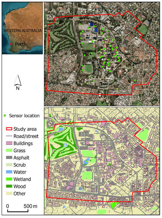
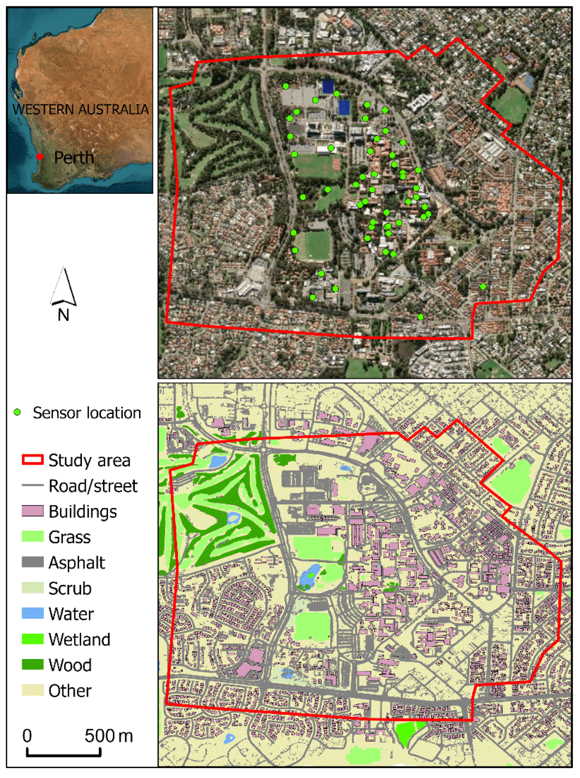
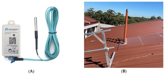
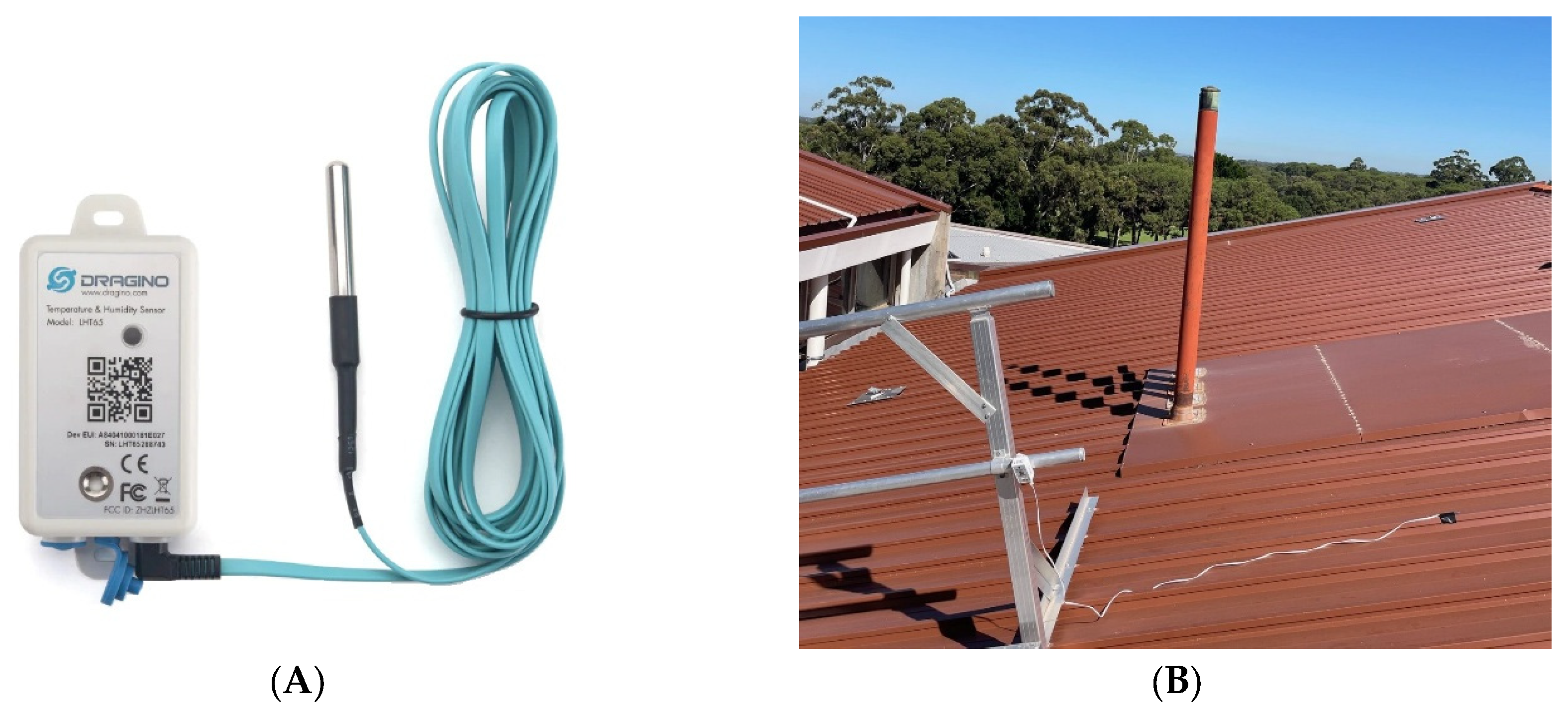
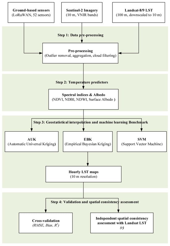
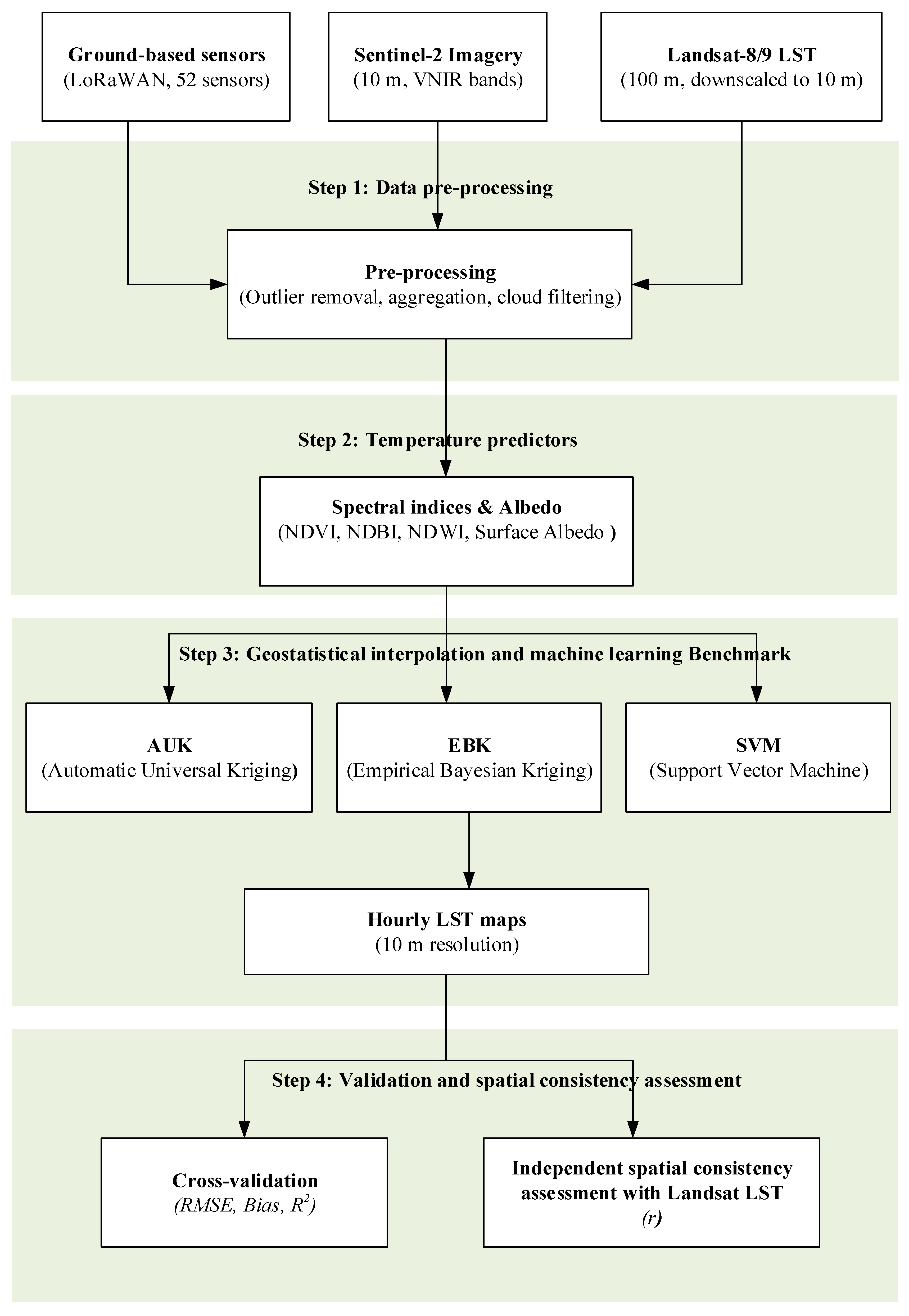
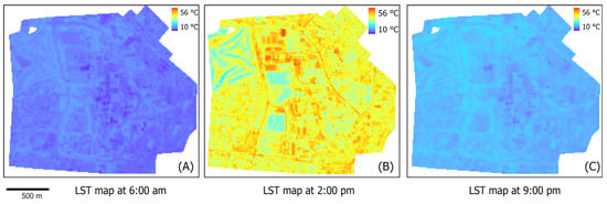
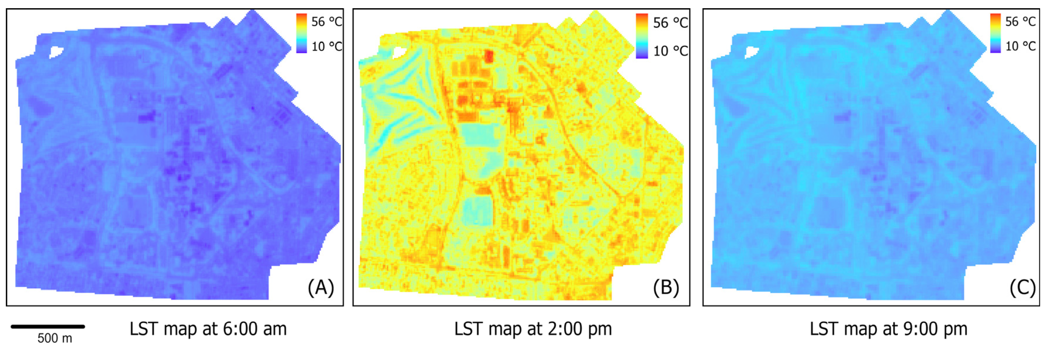
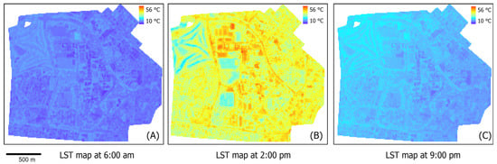
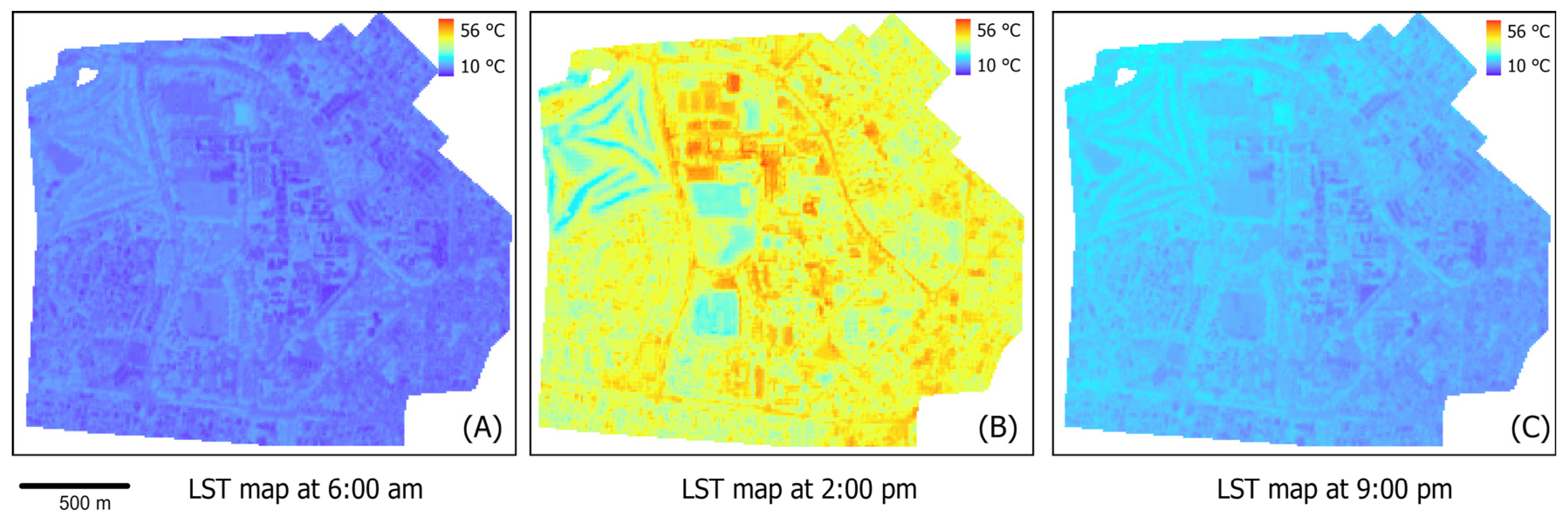
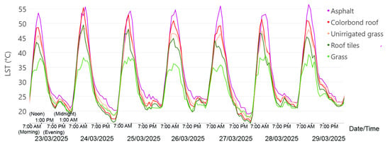
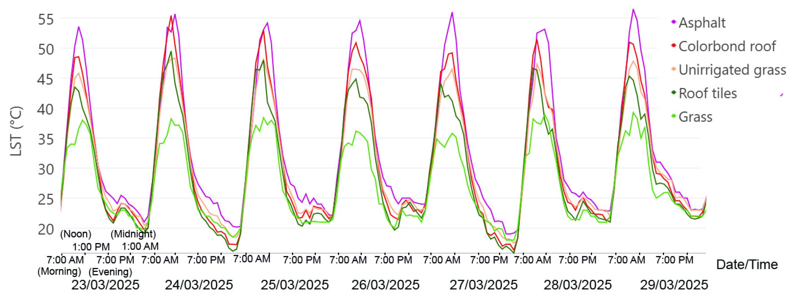
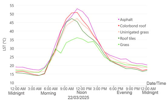
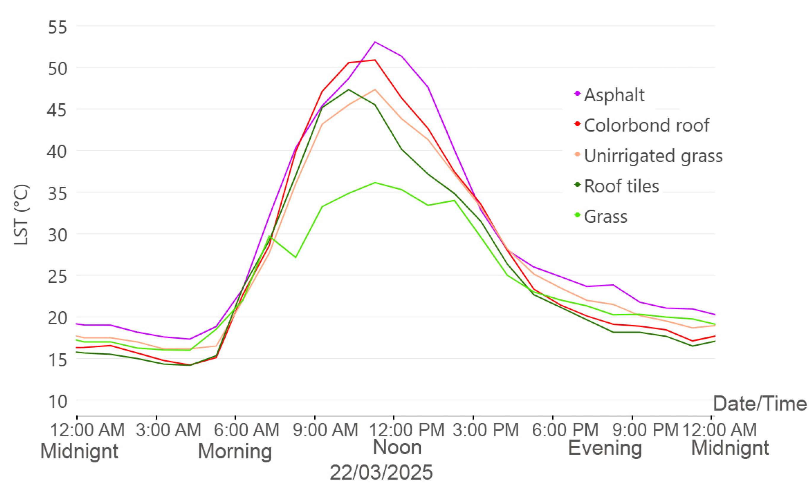
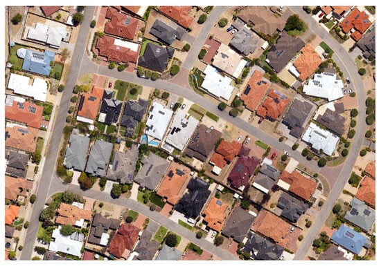
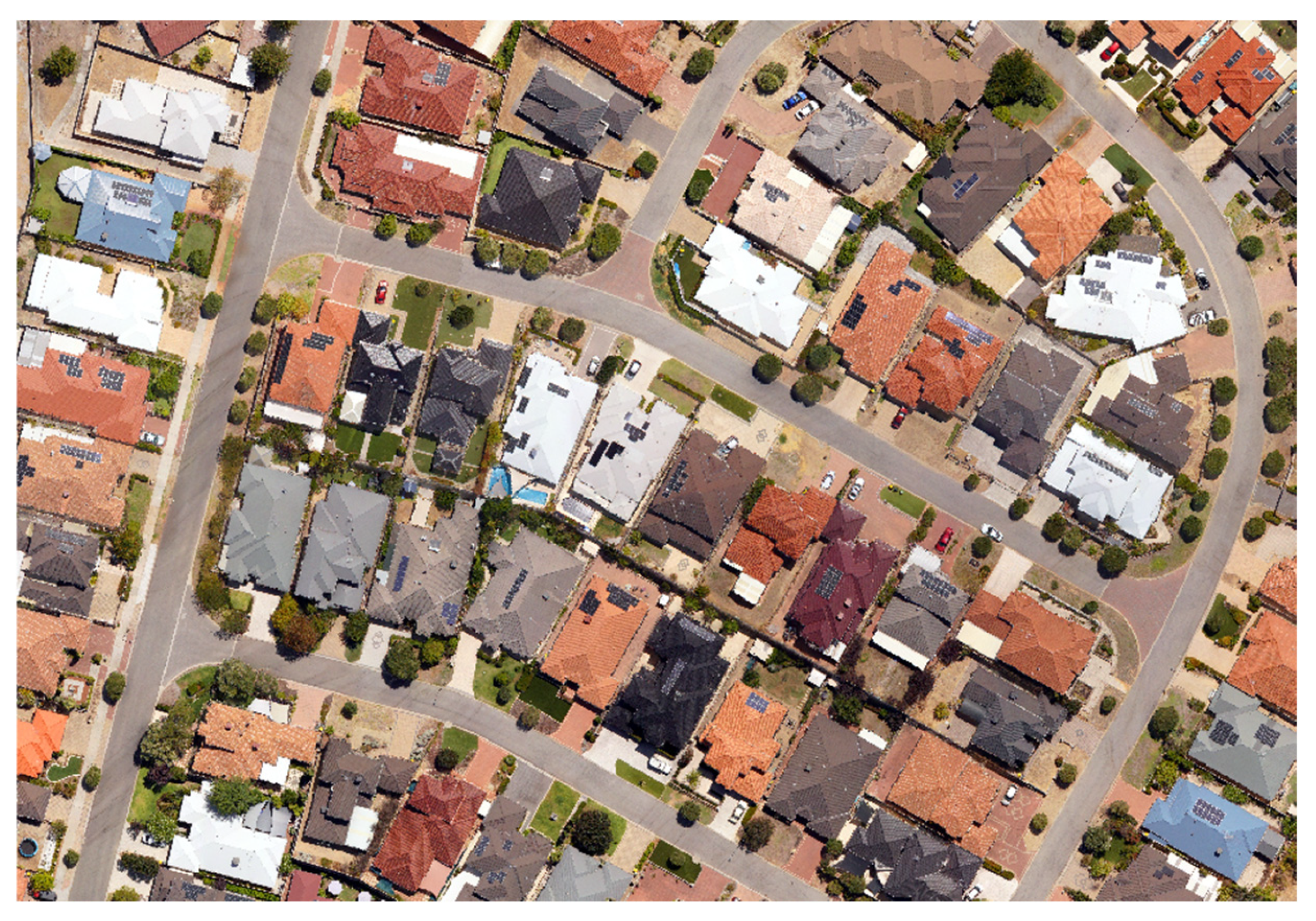

Disclaimer/Publisher’s Note: The statements, opinions and data contained in all publications are solely those of the individual author(s) and contributor(s) and not of MDPI and/or the editor(s). MDPI and/or the editor(s) disclaim responsibility for any injury to people or property resulting from any ideas, methods, instructions or products referred to in the content. |
© 2026 by the authors. Published by MDPI on behalf of the International Society for Photogrammetry and Remote Sensing. Licensee MDPI, Basel, Switzerland. This article is an open access article distributed under the terms and conditions of the Creative Commons Attribution (CC BY) license.