Geometry Guided Adaptive Ray-Surface Intersection for LiDAR Camera Fusion Spatial Localization

Abstract

In LiDAR-camera fusion measurement, conventional nearest-neighbor back-projection methods are limited by discrete point-cloud sampling and struggle to accurately recover the spatial position corresponding to image measurement points under sparse point-cloud conditions. Moreover, targets in complex industrial environments often exhibit diverse local geometric structures, making it difficult for a single surface model to effectively describe different surface characteristics. This paper proposes a Geometry-Guided Adaptive Ray-Surface Intersection measurement method, which replaces the traditional image-to-discrete-point mapping with ray-to-continuous-surface intersection. A spatial viewing ray is constructed from the image measurement point and camera optical center, and local neighborhood points are extracted through nearest projected-point back-projection. Based on curvature and normal-vector statistical features, local surfaces are classified into four geometric categories, and corresponding surface models are adaptively constructed using plane fitting, curved surface fitting, voxel-assisted plane searching, or bilinear patch fitting. The three-dimensional coordinates are then obtained through ray-model intersection. Experiments were conducted on multiple target types in an industrial equipment warehouse over a range of 5–20 m. The results show that the proposed method reduces the average measurement error from 5.63 cm of the nearest-neighbor method to 1.81 cm. When the point-cloud density decreases to 25%, the average absolute error increases by only 26.5%, compared with 92.6% and 58.7% for the nearest-neighbor and interpolation methods, respectively. These results demonstrate the effectiveness and robustness of the proposed method for LiDAR-camera fusion measurement under sparse point-cloud conditions.

1. Introduction

In complex industrial environments such as large equipment assembly workshops, preventing boundary-crossing collisions between automated suspended machinery or large robotic arms and fixed or semi-fixed equipment is a core requirement for production safety [1,2,3,4]. Such collisions can damage equipment, cause unexpected production interruptions [5,6], and even result in electrical short circuits or fires when power-related facilities, such as electrical cabinets and cable trays, are impacted. These consequences may lead to significant economic losses and safety risks. Therefore, high-precision, non-contact spatial localization of fixed and semi-fixed equipment, including electrical cabinets and processing machinery, is a prerequisite for safe automated operations [7]. However, conventional surveying methods like total stations rely on manual point-by-point operation [8,9], offering low efficiency and failing to capture dense 3D spatial information [10]. Monocular vision measurement, despite high-resolution imaging, lacks direct depth perception and suffers from poor robustness under texture-deficient or varying illumination conditions [11,12]. The fusion of LiDAR and visible-light cameras provides an effective solution [13]: LiDAR actively acquires 3D geometric information of target surfaces without being affected by illumination conditions [14], while cameras offer high angular resolution and rich texture expression capabilities, enabling precise localization of measurement points in the image plane. The two modalities exhibit strong complementarity in spatial geometry perception and visual detail representation, enabling a synergistic “LiDAR for depth, camera for positioning” measurement paradigm [15] that balances accuracy, efficiency, and robustness.

Existing LiDAR-camera fusion measurement methods in the field of industrial surveying predominantly adopt the “point cloud projection and image nearest-neighbor search” paradigm [16], which directly employs discrete LiDAR sampling points as measurement results, essentially still relying on discrete point cloud sampling. Under sparse point cloud conditions, the true spatial position corresponding to an image measurement point typically lies between adjacent LiDAR sampling points rather than coinciding exactly with a discrete point cloud. Consequently, traditional nearest-neighbor mapping methods are prone to introducing significant spatial biases. This issue is particularly pronounced in complex industrial equipment environments, where the enclosures and cables of electromechanical equipment and processing machinery exhibit complex geometric configurations. Different geometric configurations vary significantly in terms of point cloud distribution, normal variation, curvature characteristics, and surface continuity, thereby further exacerbating the measurement errors of nearest-neighbor mapping methods.

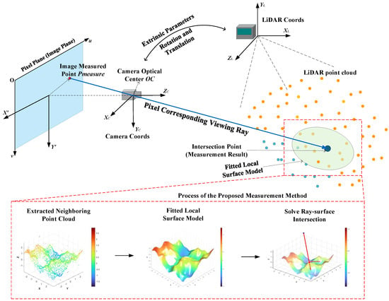
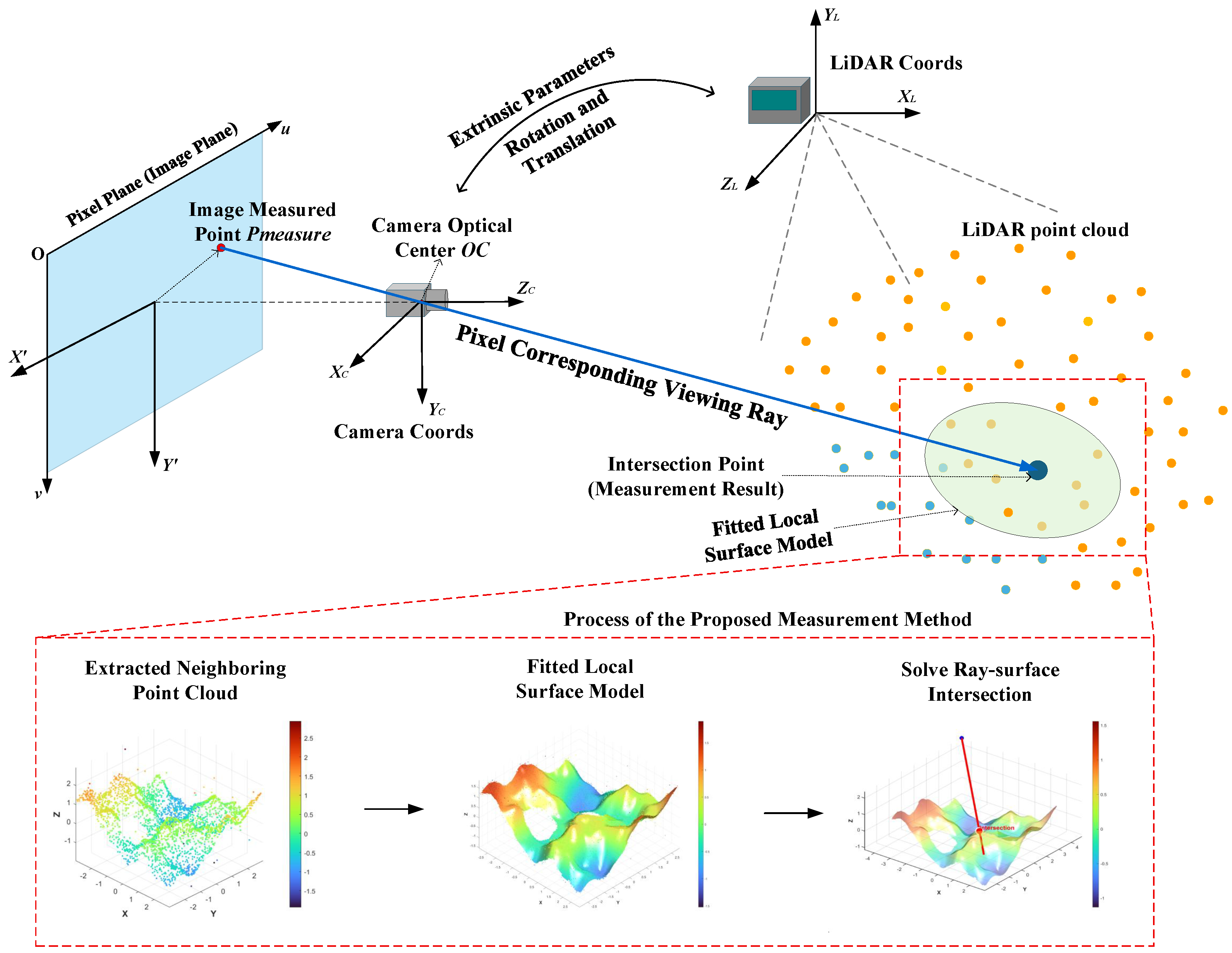
To address the above issues, this paper proposes a novel LiDAR-camera fusion measurement paradigm, termed Geometry-Guided Adaptive Ray-Surface Intersection. From the perspective of imaging geometry, the image measurement point and the camera optical center can uniquely determine a spatial line-of-sight ray [17]. The corresponding position of the image measurement point in real space should be located at the intersection of the ray and the continuous geometric surface of the target, rather than the discrete point cloud sampling point itself. Therefore, if a geometric model of the target surface can be established using the local neighborhood point cloud [18], and the measurement coordinates can be obtained by solving the intersection relationship between the spatial line-of-sight ray and the local surface, it is expected to overcome the measurement accuracy limitations caused by discrete point cloud sampling and realize the transformation from discrete point matching to continuous geometric intersection measurement. The principle is shown in Figure 1.

Figure 1. Schematic Diagram of the Geometry-Guided Adaptive Ray-Surface Intersection Method.

First, a spatial viewing ray is constructed from the image measurement point and the camera optical center, while local neighboring point clouds are extracted through nearest projected point back-projection. Subsequently, according to statistical features including local curvature, normal-vector distribution, directional entropy, and normal variation, target surfaces are classified into four categories: planar, curved, multi-plane, and scattered structures. Adaptive modeling strategies are then employed for different geometric structures, including RANSAC plane fitting [19], moving least squares (MLS) surface fitting [20], voxel-assisted plane searching, and quadrant-based bilinear patch fitting. Finally, the measurement coordinates are obtained through ray-model intersection. The main contributions of this paper are summarized as follows:

• A geometry-guided adaptive ray-surface intersection measurement framework is proposed. The proposed framework transforms conventional image-to-discrete-point mapping into ray-to-continuous-surface intersection computation, where image-derived rays intersect with locally reconstructed surfaces to obtain accurate spatial measurements.
• An adaptive point cloud fitting method for different geometric structures is developed. According to local geometric features, targets are classified into four categories: planar, curved, multi-plane, and scattered structures. Corresponding local models are established using RANSAC plane fitting, moving least squares surface fitting, voxel-assisted nearest-plane searching, and quadrant-based bilinear patch fitting, respectively.
• Experiments were conducted in an industrial equipment storage environment under multi-target conditions at measurement distances ranging from 5 m to 20 m. Experimental results demonstrate that the proposed method significantly improves measurement accuracy and robustness under sparse point cloud conditions, showing strong application potential in complex industrial equipment environments.

2. Related Works

Fusion of multi-source sensor information for high-precision spatial localization has attracted increasing attention in recent years. Wang et al. [21] fused visual and radio-frequency signals for accurate drone landing, while Zhao et al. [22] investigated LiDAR point cloud augmentation under sparse conditions. Liu et al. [23] proposed a multi-vision fusion localization framework for robust outdoor positioning. These studies demonstrate the importance of heterogeneous sensor fusion and geometric constraints for accurate localization.

Space position measurement methods based on LiDAR-camera fusion can generally be categorized into three technical approaches: back-projection methods [24], interpolation-based methods [25], and depth estimation methods [26].

Back-projection method:The 3D point cloud is projected onto the 2D image via coordinate transformation, and the resulting 2D points with color information are back-projected into 3D space. This process directly utilizes the depth information acquired by LiDAR without separate calculation of individual target points. Luo et al. [27] employed RANSAC to eliminate mismatches between 3D projection points and 2D points, and then used a direct linear solution to obtain the mapping relationship between projection points and 2D points. The study focused solely on the accuracy of back-projecting image points to the point cloud, achieving a validation accuracy of approximately 0.1 m on the dataset. However, the performance of back-projection methods highly relies on sufficient point-cloud coverage. When the point cloud is sparse, missing valid 2D–3D correspondences may lead to degraded measurement accuracy.

Interpolation method: When sparse point clouds cannot meet task requirements, interpolation techniques are typically employed to increase the amount of depth information, achieving semi-dense or even dense mapping. Common methods include nearest-neighbor interpolation [28], bilinear interpolation [29], and B-spline interpolation [30]. This approach is mainly used in object detection to obtain relatively dense depth information for one or several targets in the field of view. However, interpolation-based methods may suffer from error propagation near object boundaries, low-texture regions, and complex geometric structures.

Depth estimation method: This approach uses LiDAR and visible camera fusion devices to generate semi-dense or dense depth maps and is primarily applied in the field of 3D reconstruction. Li et al. [31] first applied a back-projection method to obtain relatively sparse fused data, then used triangulation during sensor motion to compute pixel depths without projection points, generating a dense map. Liu et al. [32] employed a cyclic candidate strategy to obtain hybrid metric-feature subgraphs from LiDAR and camera data, then generated a globally consistent metric-feature scene representation to complete the mapping between the two sensors.

From the perspective of geometric representation, ray-based modeling provides an effective connection between 2D observations and 3D structures. Hartley and Zisserman [33] established the geometric relationship between camera rays and 3D reconstruction in multi-view geometry. Recently, NeRF [34] and NeuS [35] extended ray-based representations to continuous scene modeling using radiance fields and implicit surfaces. However, these methods mainly focus on multi-view reconstruction and require dense observations or training data. They do not directly address spatial measurement from a single image observation combined with sparse LiDAR point clouds.

3. Methodology

3.1. Overall Framework

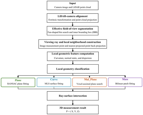
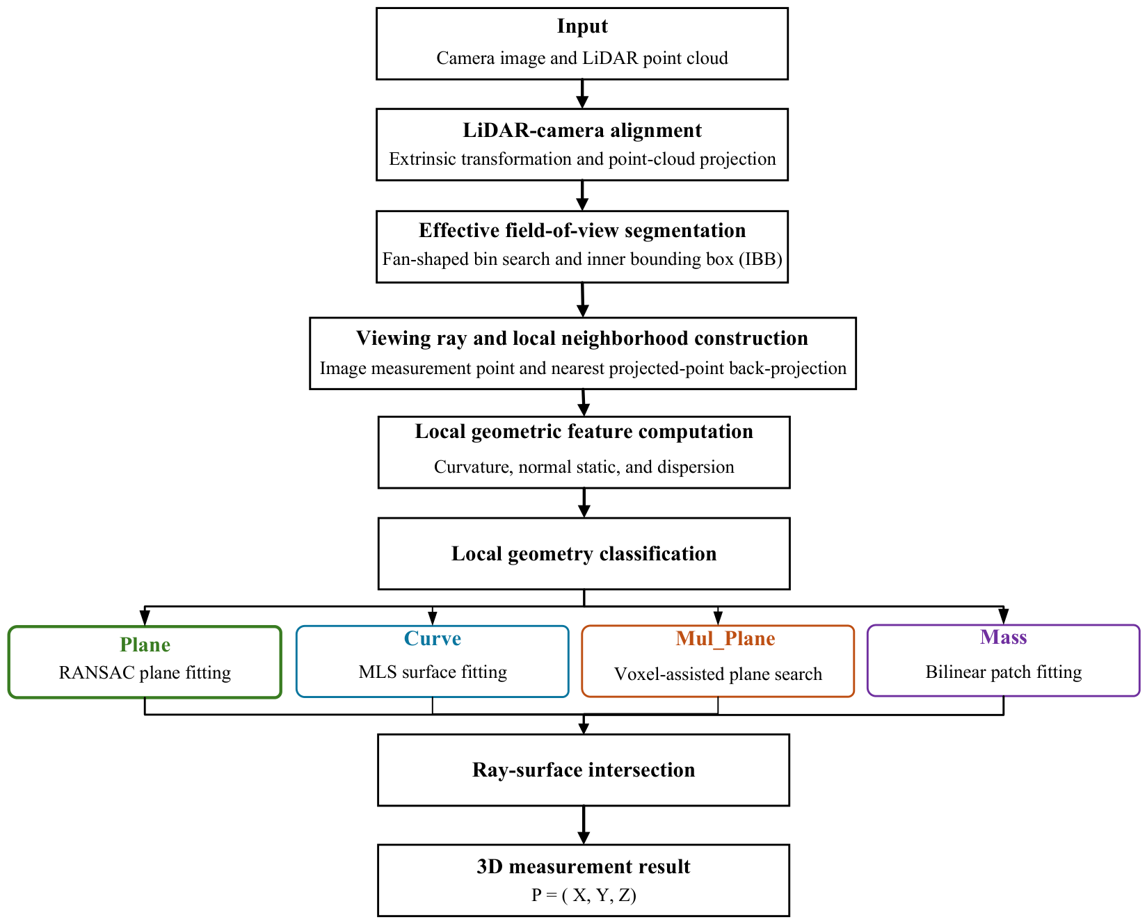
The overall framework of the proposed Geometry-Guided Adaptive Ray-Surface Intersection method is illustrated in Figure 2. The proposed method transforms conventional image-to-discrete-point mapping into ray-to-continuous-surface intersection measurement by constructing a spatial viewing ray and calculating its intersection with a local continuous surface model, thereby reducing measurement errors under sparse point cloud conditions.

Figure 2. Overall Framework of the Geometry-Guided Adaptive Ray-Surface Intersection Method.

First, the LiDAR point cloud and camera image are spatially aligned, and effective target regions are extracted using a fan-shaped search strategy and an inner bounding box (IBB), from which stable local neighboring point clouds are obtained. Subsequently, local geometric features, including curvature, normal variation, and directional entropy, are computed, and targets are classified into four categories: Plane, Curve, Mul_Plane, and Mass. According to different target types, adaptive local surface models are established using RANSAC plane fitting, moving least squares (MLS) surface fitting, voxel-assisted nearest-plane searching, and quadrant-based bilinear patch fitting, respectively. Finally, a spatial viewing ray is constructed from the image measurement point and the camera optical center, and the intersection between the ray and the local surface model is calculated to obtain the final three-dimensional measurement coordinate. Compared with conventional nearest-neighbor back-projection methods, the proposed method effectively improves measurement accuracy and robustness in complex industrial equipment environments.

3.2. Field-of-View Segmentation and Viewing Ray Construction

Before selecting image measurement points and performing ray-surface intersection calculation, it is necessary to first determine the effective overlapping region between the camera image and the projected LiDAR point cloud. Due to differences in field of view, installation position, and orientation between the LiDAR and camera, the projected three-dimensional point cloud does not necessarily cover the entire image plane. If measurement points are selected in image regions without corresponding point cloud projection support, reliable local three-dimensional neighboring point clouds cannot be obtained, which further affects subsequent surface modeling and intersection calculation. Therefore, the proposed method first extracts the effective measurement region jointly covered by both the image and the point cloud.

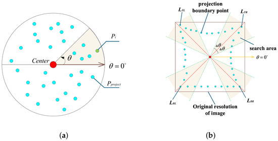
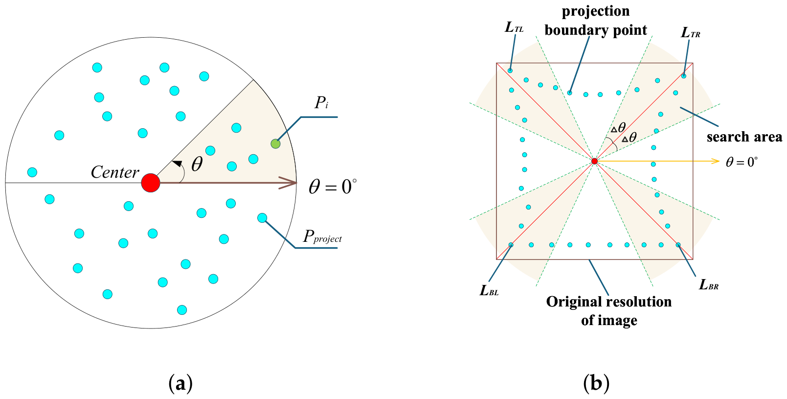
The proposed method first extracts the outer contour of the projected point set using a fan-shaped region search strategy, and then determines the IBB boundary points from four directions. Let the projected point set be denoted as $P_{\mathrm{project}}$, and the center position of the projected points be defined as $C(x_c,y_c)$. In this paper, the image center is selected as the projection center. Using the angle $\theta$ as the step size, the projected point set is divided into $360°/\theta$ fan-shaped $\mathit{bin}$ regions. During the partition process, each projected point in $P_{\mathrm{project}}$ is assigned a corresponding $\mathit{bin}$ index. The projected point set and its $\mathit{bin}$ indices are defined in Equation (1). For each projected point assigned to a bin region, the Euclidean distance between the point and the center position is calculated, and the maximum distance within each bin region is continuously updated. After all projected points in $P_{\mathrm{project}}$ are processed, the farthest point in each bin region is obtained, which is regarded as the projection boundary point. After obtaining the projection boundary point set $P_{\mathrm{bounding}}$, four corner points, including the left-top point $L_{TL}$, right-top point $L_{TR}$, left-bottom point $L_{BL}$, and right-bottom point $L_{BR}$, are further determined. An angular search threshold $\Delta \theta$ is introduced to constrain the search range, enabling corner point searching within relatively broad angular regions. The schematic diagram of the projection corner searching method is shown in Figure 3.

$$\left\{\begin{array}{c}{P}_{\mathit{project}}=\{P_1,P_2,P_3,\cdots ,P_N\}\hfill \\ \{P_i=(x_i,y_i,\mathit{bin}\_\mathit{index})\mid P_i\in P_{\mathit{project}}\}\hfill \end{array}\right.$$

(1)

Figure 3. Schematic diagram of fan-shaped bin division and corner point search. (a) Fan-shaped bin division of projected points. (b) Projected corner point search method.

After completing the field-of-view segmentation, an image measurement point located within the effective fusion region is selected as the target measurement point. Let the measurement point in the image pixel coordinate system be denoted as $P_{\mathrm{measure}}(u,v)$, where u and v represent the horizontal and vertical pixel coordinates in the image plane, respectively. According to the pinhole camera imaging model, any pixel point on the image plane and the camera optical center uniquely determine a spatial viewing ray. The normalized ray direction vector corresponding to the measurement point $P_{\mathrm{measure}}(u,v)$ can be expressed as:

$$\mathbf{v}={\left[{\displaystyle \frac{u-c_x}{f_x}},{\displaystyle \frac{v-c_y}{f_y}},1\right]}^T$$

(2)

where $c_x$ and $c_y$ denote the principal point coordinates, and $f_x$ and $f_y$ represent the normalized focal lengths obtained from the camera intrinsic parameters. The vector $\mathbf{v}$ represents the spatial direction originating from the camera optical center and passing through the image measurement point. Accordingly, the spatial viewing ray $L_m$ determined by $P_{\mathrm{measure}}$ can be expressed as:

$$L_m\left(t\right)=O_c+t\mathbf{v},t>0$$

(3)

where t is the ray parameter representing the depth value in the camera coordinate system, i.e., $t=Z_c$, and $O_c$ denotes the camera optical center. In the camera coordinate system, the optical center is defined as the coordinate origin. Therefore, Equation (3) can be further expressed as:

$$L_m\left(t\right)=t\mathbf{v}={\left[\begin{array}{ccc}t{\displaystyle \frac{u-c_x}{f_x}},\hfill & t{\displaystyle \frac{v-c_y}{f_y}},\hfill & t\hfill \end{array}\right]}^T,t>0$$

(4)

3.3. Geometry-Guided Target Surface Classification

The local geometric characteristics of the target surface directly affect the selection of point cloud fitting models and the accuracy of ray-surface intersection measurement. Local neighboring point clouds around different measurement points may exhibit varying degrees of planarity, curvature variation, normal discontinuity, and spatial discreteness. Without distinguishing local geometric structures, directly applying a unified fitting model may easily lead to model mismatch. For example, planar models cannot accurately represent continuous curved surfaces, global curved surface fitting may cross different planes in multi-plane structures, and scattered point clouds may result in unstable fitting results. Therefore, before surface modeling, the proposed method first performs geometric feature analysis and classification on the local neighboring point clouds.

In this paper, the three-dimensional point corresponding to the nearest projected point of the image measurement point is selected as the local reference point, and its neighboring point cloud is extracted for geometric analysis. Local surface characteristics are described from four aspects: local curvature, normal variation, normal-vector distribution, and depth discreteness. Local curvature reflects the degree of surface bending, normal variation characterizes the consistency or abrupt change of surface orientation, normal-vector distribution is used to determine whether multiple local surface directions exist, and depth discreteness reflects the continuity of the point cloud along the viewing direction.

3.3.1. Extraction of Target Neighboring Point Clouds

After completing fusion field-of-view segmentation and viewing ray construction, the local reference region corresponding to the image measurement point in the three-dimensional point cloud is first determined. Let the projected point set of the LiDAR point cloud on the image plane be denoted as $P_{\mathrm{project}}={\{p_i={[u_i,v_i]}^T\}}_{i=1}^M$, where each projected point $p_i$ corresponds to a three-dimensional LiDAR point. Then, the nearest projected point to the measurement point $P_{\mathrm{mea}}(u,v)$ is searched in the image plane as follows:

$$p_{\mathrm{near}}=\arg \underset{p_i\in P_{\mathrm{project}}}{\min }{∥p_i-P_{\mathrm{mea}}∥}_2$$

(5)

The three-dimensional point corresponding to the nearest projected point $p_{\mathrm{near}}$ is denoted as:

$$P_{\mathrm{ref}}={\left[X_{\mathrm{ref}},Y_{\mathrm{ref}},Z_{\mathrm{ref}}\right]}^T$$

(6)

In this paper, $P_{\mathrm{ref}}$ is not directly used as the final measurement result, but instead serves as a local reference point for extracting neighboring target point clouds around the measurement point. Taking $P_{\mathrm{ref}}$ as the center, the neighboring point cloud in the three-dimensional space is searched as follows:

$$\mathcal{N}\left(P_{\mathrm{ref}}\right)=\left\{P_j\in \mathcal{P}\mid {∥P_j-P_{\mathrm{ref}}∥}_2\le r\right\}$$

(7)

where $\mathcal{P}$ denotes the original LiDAR point cloud set, and r represents the neighborhood search radius. The extracted neighboring point cloud is then used as the input for subsequent geometric feature computation and target surface classification.

3.3.2. Local Surface Type Determination

Curvature reflects the bending degree of the local surface, while normal vectors describe local surface orientation. For planar regions, neighboring point clouds usually exhibit low curvature and stable normal vectors. For curved regions, curvature may increase, while normal variation remains relatively continuous. For multi-plane or scattered targets, normal-vector distributions often present abrupt changes, discrete distributions, or multi-directional characteristics. Therefore, the covariance matrix of the neighboring point cloud $\mathcal{N}\left(P_{\mathrm{ref}}\right)$ obtained in Section 3.3.1 is constructed as follows:

$$C={\displaystyle \frac{1}{n}}{\displaystyle \sum _{i=1}^n}(P_i-\overline{P}){(P_i-\overline{P})}^T$$

(8)

where $\overline{P}$ denotes the centroid of $\mathcal{N}\left(P_{\mathrm{ref}}\right)$. Eigenvalue decomposition is then performed on the covariance matrix C to obtain three eigenvalues ${\lambda }_1$, ${\lambda }_2$, and ${\lambda }_3$, where ${\lambda }_1>{\lambda }_2>{\lambda }_3$. These eigenvalues represent the spatial distribution of the neighboring point cloud along the principal direction, secondary principal direction, and normal direction, respectively. Based on the eigenvalues, the local curvature index can be defined as:

$$\kappa ={\displaystyle \frac{{\lambda }_3}{{\lambda }_1+{\lambda }_2+{\lambda }_3}}$$

(9)

The local normal vector is represented by the eigenvector corresponding to the smallest eigenvalue ${\lambda }_3$, i.e., $\mathbf{n}={\mathbf{e}}_3$. The normal vector set can then be expressed as:

$${\mathcal{N}}_{\mathrm{normal}}={\left\{{\mathbf{n}}_i\right\}}_{i=1}^n$$

(10)

where ${\mathbf{n}}_i$ denotes the local normal vector of the i-th neighboring point. Compared with a single normal vector, the overall distribution of neighboring normal vectors can better characterize local surface structures. For planar regions, normal vectors are usually concentrated in a single direction. For continuous curved surfaces, normal vectors change smoothly with surface curvature. For multi-plane structures, multiple dominant normal directions often exist simultaneously, while scattered regions usually exhibit highly discrete and irregular normal-vector distributions.

To quantitatively characterize the directional distribution of normal vectors, the neighboring normal vectors are mapped into an angular statistical space, and a normal-vector direction histogram is constructed. Assuming that the histogram contains m bins and the number of normal vectors within the k-th bin is denoted as $h_k$, the normalized probability can be expressed as:

$$p_k={\displaystyle \frac{h_k}{{\sum }_{k=1}^m{h}_k}}$$

(11)

Based on the above probability distribution, the normal-vector directional entropy is defined as:

$$H=-{\displaystyle \sum _{k=1}^m}{p}_k\log \left(p_k\right)$$

(12)

When the normal-vector directions are concentrated within a few bins, the entropy value H is relatively low, indicating strong local surface orientation consistency. In contrast, when the normal-vector directions are more widely distributed, the entropy value H becomes higher, implying significant local surface direction variation or irregular distribution. Meanwhile, the number of peaks $N_p$ in the normal-vector direction histogram is also calculated to characterize the number of dominant surface orientations within the neighborhood. When $N_p=1$, the local normal vectors are mainly concentrated around a single direction, indicating strong surface consistency. When $N_p>1$, multiple dominant normal directions may exist within the neighborhood.

Furthermore, to describe the overall variation of normal-vector directions, the standard deviation of the normal-vector orientation angles is calculated as:

$${\sigma }_n=\sqrt{{\displaystyle \frac{1}{n}}\sum _{i=1}^n{({\theta }_i-\overline{\theta })}^2}$$

(13)

where ${\mathbf{n}}_i={(n_x^i,n_y^i,n_z^i)}^T$ denotes the i-th normal vector obtained through covariance analysis. The orientation angle of the normal vector is calculated as ${\theta }_i=\mathrm{atan2}(n_y^i,n_x^i)$, where ${\theta }_i$ represents the angular representation of the i-th normal vector in the directional statistical space, and $\overline{\theta }$ represents the mean orientation angle of neighboring normal vectors.

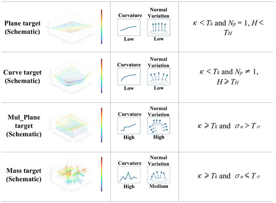
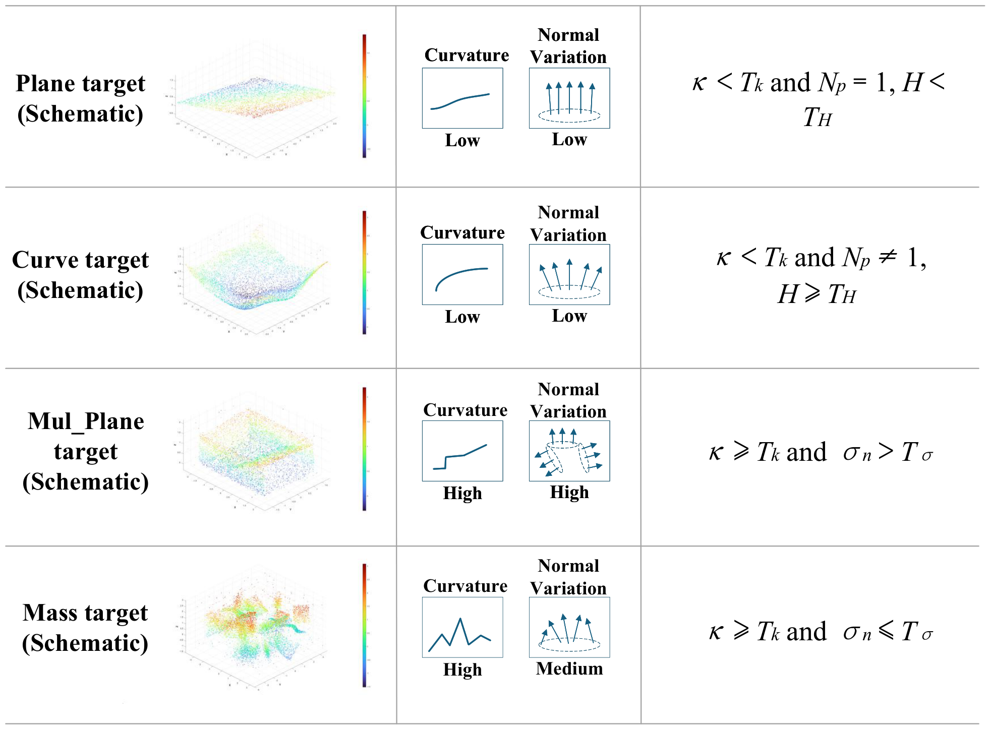
Based on the above geometric statistical features, a coarse-to-fine strategy is adopted to determine the local surface type. First, the local curvature is used to determine whether the neighboring region belongs to a low-curvature surface. Let the curvature threshold be denoted as $T_{\kappa }$. When $\kappa <T_{\kappa }$, the local surface exhibits low bending variation, and the neighboring point cloud is more likely to correspond to a planar or smoothly varying curved surface. For such low-curvature regions, the number of normal-vector peaks and the entropy value are further used to determine whether the local surface can be stably represented by a single plane. Let the entropy threshold be denoted as $T_H$. When

$$N_p=1,H<T_H$$

(14)

the normal-vector directions are concentrated with strong orientation consistency, and the local point cloud is classified as a Plane target. Otherwise, although the overall curvature remains low, the normal-vector directions exhibit continuous variation or certain discreteness, indicating that a single planar model cannot adequately describe the local surface geometry. Therefore, the local surface is classified as a Curve target.

When the local curvature satisfies $\kappa \ge T_{\kappa }$, the neighboring region exhibits significant surface fluctuation, edge structures, or irregular distributions. For such high-curvature regions, the standard deviation of normal-vector directions is further used to determine whether multiple dominant surface orientations exist. Let the standard deviation threshold be denoted as $T_{\mathrm{std}}$. When

$${\sigma }_n>T_{\mathrm{std}}$$

(15)

the normal-vector directions vary significantly within the neighborhood, indicating that the local region may consist of multiple adjacent planar patches. Therefore, the target is classified as a multi-plane structure. Otherwise, although the curvature remains relatively high, the normal-vector distribution does not exhibit stable multi-directional characteristics, and the spatial distribution of the point cloud is more likely to be irregular or scattered. Since such local surfaces cannot be stably represented by either a single plane or a continuous curved surface, the target is classified as a Mass target.

In summary, the local neighboring surface of the measurement point is classified into four categories: Plane, Curve, Mul_Plane, and Mass. Corresponding adaptive ray-surface intersection strategies are then designed for different target types. The relationship between target surface geometric characteristics and the corresponding measurement strategies is illustrated in Figure 4. The classification algorithm is shown in Algorithm 1.

Algorithm 1 Local Surface Type Determination

Require: $\mathcal{N}\left(P_{\mathrm{ref}}\right)$ (local point cloud) Ensure: $T\in \{\mathrm{Plane},\mathrm{Curve},\mathrm{Mul}\_\mathrm{Plane},\mathrm{Mass}\}$  Compute covariance C and eigenvalues ${\lambda }_1\ge {\lambda }_2\ge {\lambda }_3$  $\kappa ={\lambda }_3/({\lambda }_1+{\lambda }_2+{\lambda }_3)$  Compute normals and histogram $\left\{h_k\right\}$, entropy H, peak count $N_p$, std ${\sigma }_n$  if  $\kappa <T_{\kappa }$  then        if $N_p=1$ and $H<T_H$ then $T\leftarrow \mathrm{Plane}$        else $T\leftarrow \mathrm{Curve}$  else        if ${\sigma }_n>T_{\mathrm{std}}$ then $T\leftarrow \mathrm{Mul}\_\mathrm{Plane}$        else $T\leftarrow \mathrm{Mass}$  return  T

Figure 4. Four Classification Categories and Their Geometric Characteristics.

3.4. Adaptive Ray-Surface Intersection Strategy

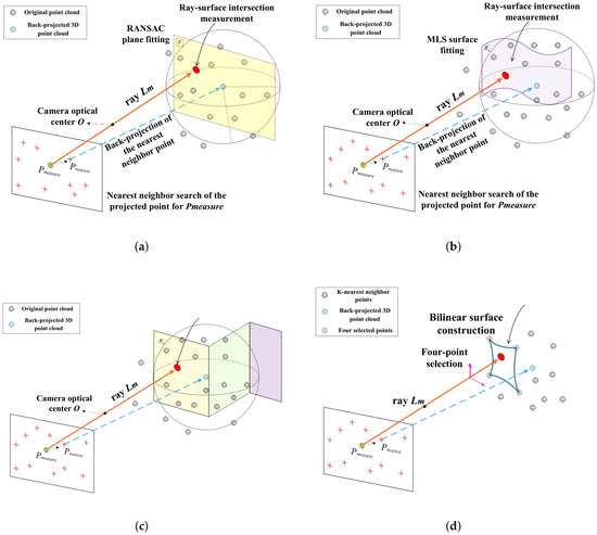
After determining the local surface type, corresponding local surface modeling strategies are selected according to different geometric characteristics, and the intersection between the camera viewing ray and the local surface model is calculated. Specifically, planar targets correspond to plane-based measurement, curved targets correspond to surface-based measurement, multi-plane targets correspond to multi-plane measurement, and scattered targets correspond to single-point measurement. The schematic diagram of the proposed adaptive ray-surface intersection strategies is shown in Figure 5.

Figure 5. Schematic Diagram of Measurement Methods. (a) Principle of the Plane target measurement mode. (b) Principle of the Curve target measurement mode. (c) Principle of the Mul_Plane target measurement mode. (d) Principle of the Mass target measurement mode.

3.4.1. Plane Target Measurement

For plane targets, the neighboring point cloud around the measurement point usually exhibits low curvature, stable normal vectors, and strong planar consistency. Therefore, a planar model can be used to describe the local target surface. Considering that low-cost LiDAR point clouds may contain outliers, boundary points, and local noise, RANSAC plane fitting is adopted to improve the robustness of plane parameter estimation. Meanwhile, to prevent the intersection point between the viewing ray and the fitted plane from falling outside the valid target region, the Alpha Shape method [36] is introduced to constrain the local point cloud boundary, and only intersection results located within the effective target boundary are retained. The schematic diagram of the proposed plane target measurement strategy is shown in Figure 5a.

In the LiDAR coordinate system, the plane equation obtained through RANSAC plane fitting is expressed as $A_{L}x+B_{L}y+C_{L}z+D_L=0$, where the corresponding plane normal vector is ${\mathbf{n}}_L={[A_L,B_L,C_L]}^T$, and $(x,y,z)$ denotes the coordinates of a three-dimensional point in the LiDAR coordinate system. Based on the extrinsic calibration parameters, the rotation matrix $R_{CL}$ and translation vector $t_{CL}$ from the LiDAR coordinate system to the camera coordinate system can be obtained. Accordingly, the plane normal vector and plane parameter in the camera coordinate system are given by ${\mathbf{n}}_C=R_{CL}{\mathbf{n}}_L$ and $D_C=D_L-{\mathbf{n}}_C^T{t}_{CL}$, respectively. Thus, the plane equation in the camera coordinate system can be expressed as

$${\mathbf{n}}_C^T{X}_C+D_C=0$$

(16)

where ${\mathbf{n}}_C$ denotes the plane normal vector in the camera coordinate system, $D_C$ represents the constant term of the plane equation, and $X_C={(x_C,y_C,z_C)}^T$ denotes the three-dimensional point coordinates in the camera coordinate system. Therefore, the plane equation in the camera coordinate system can also be written as

$$A_{C}x+B_{C}y+C_{C}z+D_C=0$$

(17)

Substituting the viewing ray equation constructed in Section 3.2,

$$L_m\left(t\right)=t\mathbf{v}={\left[t{\displaystyle \frac{u-c_x}{f_x}},t{\displaystyle \frac{v-c_y}{f_y}},t\right]}^T$$

(18)

into the plane equation in the camera coordinate system yields

$$A_C\left(t{\displaystyle \frac{u-c_x}{f_x}}\right)+B_C\left(t{\displaystyle \frac{v-c_y}{f_y}}\right)+C_{C}t+D_C=0$$

(19)

The depth value $t^{\ast }$ of the ray-plane intersection point can then be obtained as

$$t^{\ast }=-{\displaystyle \frac{D_C}{A_C\frac{u-c_x}{f_x}+B_C\frac{v-c_y}{f_y}+C_C}}$$

(20)

The depth value $t^{\ast }$ represents the intersection depth of the viewing ray. To ensure that the intersection point lies within the valid target region, the Alpha Shape method [36] is further employed to constrain the boundary of the local planar point cloud. Specifically, the planar neighboring points are projected onto the two-dimensional local coordinate system of the fitted plane to obtain the two-dimensional point set $Q_{\mathrm{plane}}={\left\{q_i\right\}}_{i=1}^n$. Based on $Q_{\mathrm{plane}}$, the Alpha Shape boundary $B_{\alpha }$ is constructed. If the projected two-dimensional coordinate of the intersection point, denoted as $q_{\mathrm{int}}$, satisfies $q_{\mathrm{int}}\in B_{\alpha }$, the intersection point $P_{\mathrm{int}}$ is considered to lie within the valid target region and is retained as the final measurement result.

3.4.2. Curve Target Measurement

For curved targets, the local neighboring point cloud usually exhibits continuous curvature variation and smooth normal-vector changes, making a single planar model insufficient to accurately describe the local surface geometry. Therefore, the proposed method adopts the Moving Least Squares (MLS) method to construct a local continuous curved surface model, while the Alpha Shape constraint is further introduced to preserve the effective target boundary, as illustrated in Figure 5b.

A quadratic surface with ten coefficients is employed to represent the local curved surface:

$$\mathsf{\Phi }(x,y,z)=a_1{x}^2+a_2{y}^2+a_3{z}^2+a_{4}xy+a_{5}xz+a_{6}yz+a_{7}x+a_{8}y+a_{9}z+a_{10}=0$$

(21)

where

$$\mathbf{a}={[a_1,a_2,\cdots ,a_{10}]}^T$$

(22)

is the quadratic surface parameter vector. The surface parameters are estimated using weighted least squares:

$$\underset{\mathbf{a}}{\min }{\displaystyle \sum _{j=1}^{n_{\mathrm{fit}}}}\theta \left(d_j\right){\left[\mathsf{\Phi }(x_j,y_j,z_j)\right]}^2$$

(23)

where $\theta \left(d_j\right)$ denotes the MLS distance weighting function, $d_j$ represents the distance from point $p_j$ to the local reference point, and h is the smoothing parameter. The weighting function is defined as

$$\theta \left(d_j\right)=\exp \left(-{\displaystyle \frac{d_j^2}{h^2}}\right)$$

(24)

where h is the smoothing parameter in the moving least squares formulation. It is determined according to the local neighborhood radius r as $h=\alpha r$, where $\alpha$ is a scale coefficient. The viewing ray can be expressed as

$$L_m\left(t\right)={[x\left(t\right),y\left(t\right),z\left(t\right)]}^T$$

(25)

Substituting the viewing ray into the quadratic surface equation yields

$$\mathsf{\Phi }\left(x\right(t),y(t),z(t\left)\right)=0$$

(26)

Since $x\left(t\right)$, $y\left(t\right)$, and $z\left(t\right)$ are all linear functions of t, Equation (26) can be transformed into a one-dimensional quadratic equation with respect to t:

$$a_t{t}^2+b_{t}t+c_t=0$$

(27)

After solving for the valid intersection parameter $t^{\ast }$, the intersection point of the curved target is obtained as

$$P_{\mathrm{int}}=L_m\left(t^{\ast }\right)$$

(28)

3.4.3. Mul_Plane Target Measurement

First, the neighboring target point cloud is voxelized to balance point cloud density and reduce the influence of local noise. Subsequently, candidate local planar patches are extracted from the voxelized point cloud, and RANSAC is employed to estimate each candidate plane model ${\pi }_j:a_{j}x+b_{j}y+c_{j}z+d_j=0$, where j denotes the index of the j-th candidate plane. To determine the plane most relevant to the viewing ray, the intersection between the ray and each candidate plane is calculated. For the candidate plane ${\pi }_j$, the intersection parameter is computed as

$$t_j=-{\displaystyle \frac{a_j{X}_C+b_j{Y}_C+c_j{Z}_C+d_j}{a_j{v}_x+b_j{v}_y+c_j{v}_z}}$$

(29)

where $(X_C,Y_C,Z_C)$ denotes the camera optical center and $(v_x,v_y,v_z)$ represents the viewing ray direction vector.

To avoid invalid intersections caused by plane extrapolation, the effective plane is selected according to the spatial proximity between the intersection point and the corresponding planar point set. Let the point set corresponding to the j-th plane be denoted as ${\mathcal{S}}_j$. The distance from the intersection point to the planar patch is defined as

$$D_j=\underset{P_i\in {\mathcal{S}}_j}{\min }{∥P_j-P_i∥}_2$$

(30)

Among candidate planes satisfying both boundary constraints and valid intersection conditions, the plane with the minimum $D_j$ is selected as the final intersection plane:

$$j^{\ast }=\arg \underset{j}{\min }{D}_j,P_{\mathrm{int}}=P_{j^{\ast }}$$

(31)

3.4.4. Mass Target Measurement

Scattered targets usually do not exhibit clear geometric characteristics such as planar or curved structures, and their neighboring point clouds are often irregularly distributed and spatially discrete. Therefore, instead of directly performing global surface fitting, the proposed method first applies K-nearest neighbor (KNN) searching to extract neighboring points and transforms them into the camera coordinate system. A local coordinate system is then constructed based on the viewing ray direction for single-point measurement.

Specifically, the viewing ray direction vector $\mathbf{v}$ is taken as the local coordinate system normal direction. To avoid the reference direction becoming parallel to the viewing ray, the reference vector ${\mathbf{r}}_0$ is selected as

$${\mathbf{r}}_0=\left\{\begin{array}{cc}{[1,0,0]}^T,\hfill & \left|\mathbf{v}·{[1,0,0]}^T\right|\le 0.9\hfill \\ {[0,1,0]}^T,\hfill & \left|\mathbf{v}·{[1,0,0]}^T\right|>0.9\hfill \end{array}\right.$$

(32)

where the dot product represents the cosine of the angle between two vectors, and the threshold value $0.9$ is used to prevent the reference direction from becoming parallel to the local coordinate axes. The orthogonal basis vectors of the local coordinate system are constructed as

$${\mathbf{x}}_{\mathrm{local}}={\displaystyle \frac{{\mathbf{r}}_0\times \mathbf{v}}{∥{\mathbf{r}}_0\times \mathbf{v}∥}}$$

(33)

$${\mathbf{y}}_{\mathrm{local}}=\mathbf{v}\times {\mathbf{x}}_{\mathrm{local}}$$

(34)

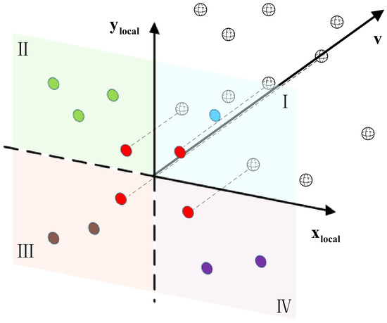
After constructing the local coordinate system, the neighboring points are projected onto the local $XOY$ plane and divided into four quadrants. The farthest neighboring point in each quadrant is selected to form four representative control points. If one or more quadrants contain no neighboring points, the measurement is considered invalid, indicating that the target point distribution is excessively sparse and the neighborhood size K should be increased. The schematic diagram of the proposed point selection strategy is shown in Figure 6.

Figure 6. Four selected points.

Based on the four selected three-dimensional control points $P_{00}$, $P_{10}$, $P_{01}$, and $P_{11}$, a local bilinear surface patch is constructed as

$$S(\xi ,\eta )=(1-\xi )(1-\eta )P_{00}+\xi (1-\eta )P_{10}+(1-\xi )\eta P_{01}+\xi \eta P_{11}$$

(35)

where $0\le \xi \le 1$ and $0\le \eta \le 1$. Substituting the viewing ray equation into the bilinear surface equation yields the final intersection point:

$$P_{\mathrm{int}}=O_C+t^{\ast }\mathbf{v}$$

(36)

The proposed method constructs a local coordinate system orthogonal to the viewing ray and establishes a local bilinear surface patch using representative neighboring points selected from four quadrants. Compared with global fitting methods, the proposed strategy achieves more stable single-point measurement results under scattered point cloud conditions while reducing overfitting caused by irregular point distributions.

4. Experiments and Results

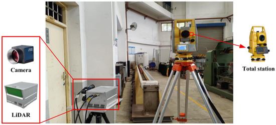
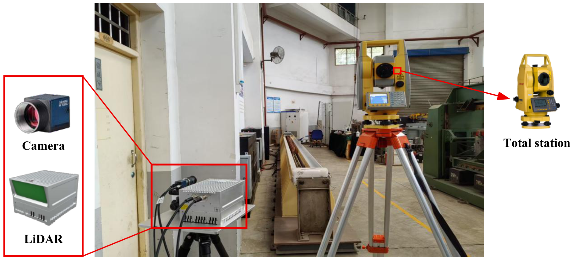
The LiDAR used in the experiments is the Benewak Horn-X2 Pro (Benewake, Beijing, China), while the camera is the MER2-231-41GM/C (DAHENG IMAGING, Beijing, China). An NTS-382R10 (South Surveying and Mapping, Guangzhou, China) total station is employed as the ground-truth measurement device. The computation platform is equipped with an AMD Ryzen 9 7945HX processor (AMD, Santa Clara, CA, USA), 16 GB memory, and an NVIDIA GeForce RTX 4060 GPU. All algorithms are implemented in C++. The experimental devices are shown in Figure 7. The LiDAR-camera extrinsic calibration is performed using the integrated calibration method proposed by Chen et al. [37]. The obtained extrinsic parameters are given in Equation (37), and the average reprojection error of the extrinsic calibration is 1.78 pixels.

$$R=\left[\begin{array}{ccc}-0.057414& -0.997805& 0.033007\\ 0.028291& -0.034674& -0.998998\\ 0.997949& -0.056424& 0.030220\end{array}\right],t=\left[\begin{array}{c}0.258389\\ 0.060253\\ -0.052010\end{array}\right]$$

(37)

Figure 7. Deployment Diagram of the LiDAR, Camera, and Total Station in the Experiment.

4.1. Geometry-Guided Target Classification Experiment

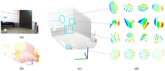
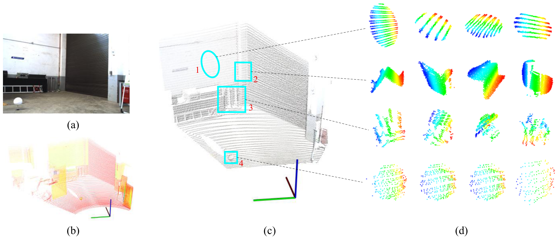
To validate the effectiveness of the proposed target surface classification method, field experiments were conducted in an industrial equipment storage environment. As shown in Figure 8, a flat wall surface, door-frame corner, randomly stacked objects, and a spherical target were selected for quantitative classification experiments, corresponding to targets 1, 2, 3, and 4, respectively.

Figure 8. Field Experiment for Target Classification. (a) Experimental Scene Image. (b) Experimental Scene Point Cloud. (c) Effective Operating Region After Field-of-View Segmentation. (d) Partial Point Cloud.

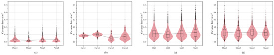
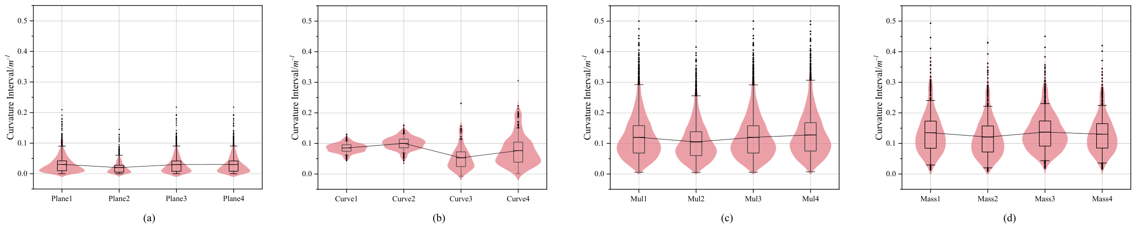
First, the flat wall surface, door-frame corner, randomly stacked objects, and spherical target were manually classified as Plane, Mul_Plane, Mass, and Curve targets, respectively. Subsequently, curvature statistics were performed for the four target types, as illustrated in Figure 9.

Figure 9. Relationship between curvature distribution and geometric classification. (a) Relationship between curvature distribution and the Plane classification. (b) Relationship between curvature distribution and the Curve classification. (c) Relationship between curvature distribution and the Mul_Plane classification. (d) Relationship between curvature distribution and the Mass classification.

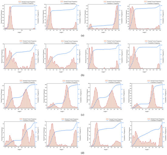
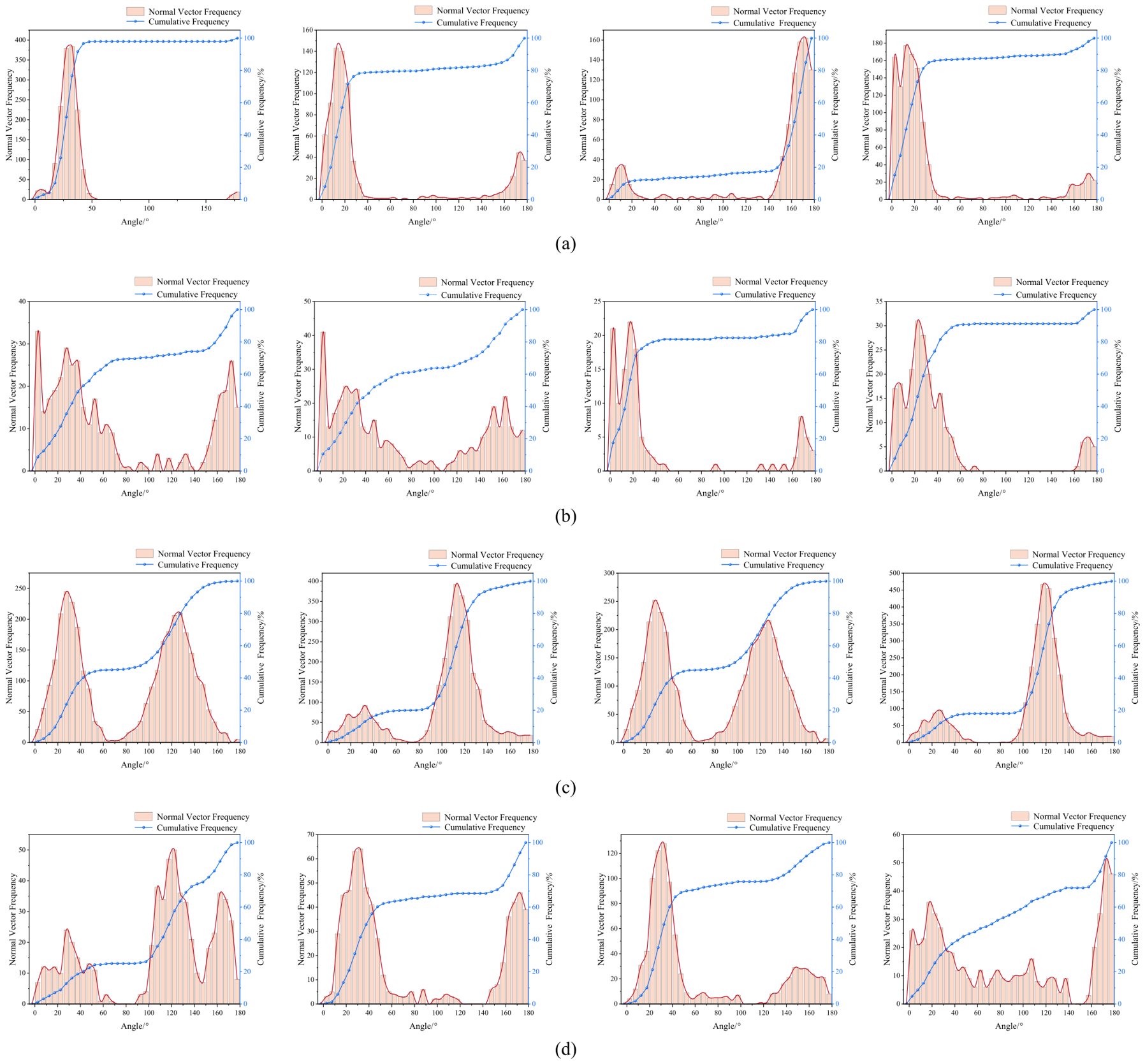
As shown in the curvature statistics in Figure 9, the curvature distributions of Plane and Curve targets mainly exhibit single-peak distributions within the range of $[0,0.20]{\mathrm{m}}^{-1}$, where most neighboring points are concentrated and the mean curvature values remain below $0.10{\mathrm{m}}^{-1}$. In contrast, the curvature distributions of Mul_Plane and Mass targets are more dispersed, and their mean curvature values are generally greater than $0.10{\mathrm{m}}^{-1}$. Therefore, by setting a curvature threshold, the targets can first be divided into two categories: Plane/Curve and Mul_Plane/Mass. In this paper, the curvature threshold is set as $T_{\kappa }=0.1$. Subsequently, normal-vector statistics are further performed for the four target types, as illustrated in Figure 10.

Figure 10. Normal-vector orientation distributions of local point clouds for different geometric categories: (a) Plane targets, (b) Curve targets, (c) Multi-plane targets, and (d) Mass targets.

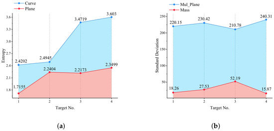
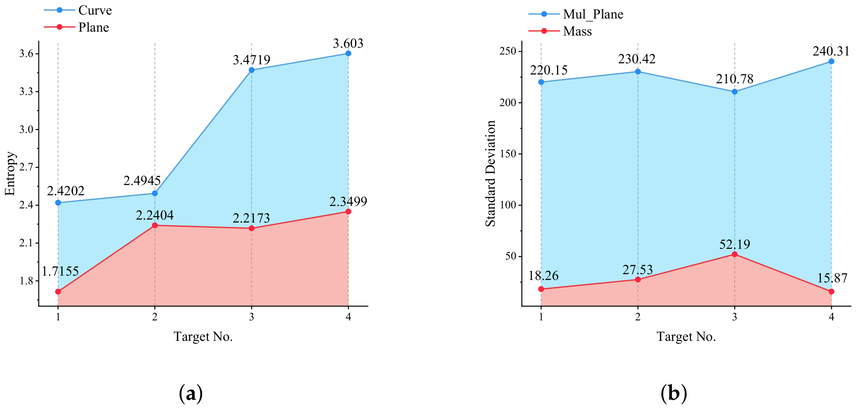
Based on the local normal-vector statistics, the normal-vector directional entropy distributions of Plane and Curve targets are shown in Figure 11a. The entropy values of Curve targets are significantly higher than those of Plane targets, and the entropy threshold is therefore set to 2.5. The standard deviation distributions of Mul_Plane and Mass targets are shown in Figure 11b. The standard deviation values of Mul_Plane targets are significantly higher than those of Mass targets, and the corresponding threshold is set to 70.

Figure 11. Statistical characteristics of normal-vector distributions for different geometric categories. (a) Entropy values of normal-vector distributions for Plane and Curve targets. (b) Standard deviation of normal-vector directions for Mul_Plane and Mass targets. The target number (1–4) indicates different test samples within the same geometric category.

4.2. Measurement Accuracy Comparison

To evaluate the measurement accuracy of the proposed method, a total station was employed to obtain the spatial coordinates of measurement points in the total station coordinate system. In this experiment, the total station measurements were regarded as ground truth. Since transforming LiDAR coordinates into the total station coordinate system may introduce additional transformation errors, relative distance comparison was adopted for accuracy evaluation. Specifically, point 1 was selected as the reference point, and the relative distances from all other points to point 1 were calculated. Let the ground-truth coordinates measured by the total station be denoted as $P_i^{gt}=(X_i^{gt},Y_i^{gt},Z_i^{gt})$, and the measured coordinates be denoted as $P_i^m=(X_i^m,Y_i^m,Z_i^m)$. Using point 1 as the reference point, the ground-truth relative distance from the i-th point to point 1 is calculated as $D_i^{gt}={∥P_i^{gt}-P_1^{gt}∥}_2$, while the measured relative distance is given by $D_i^m={∥P_i^m-P_1^m∥}_2$. The distance error is then defined as $e_i=D_i^m-D_i^{gt}$. This metric evaluates the end-to-end spatial measurement capability of the proposed method and is consistent with the practical requirements of industrial equipment measurement and collision prevention, where the relative spatial relationship between objects is more critical than their absolute positions in a global coordinate frame. It should be noted that relative-distance accuracy does not fully represent absolute 3D localization accuracy, which requires a unified coordinate registration framework and additional calibration evaluation.

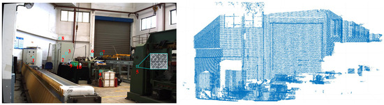
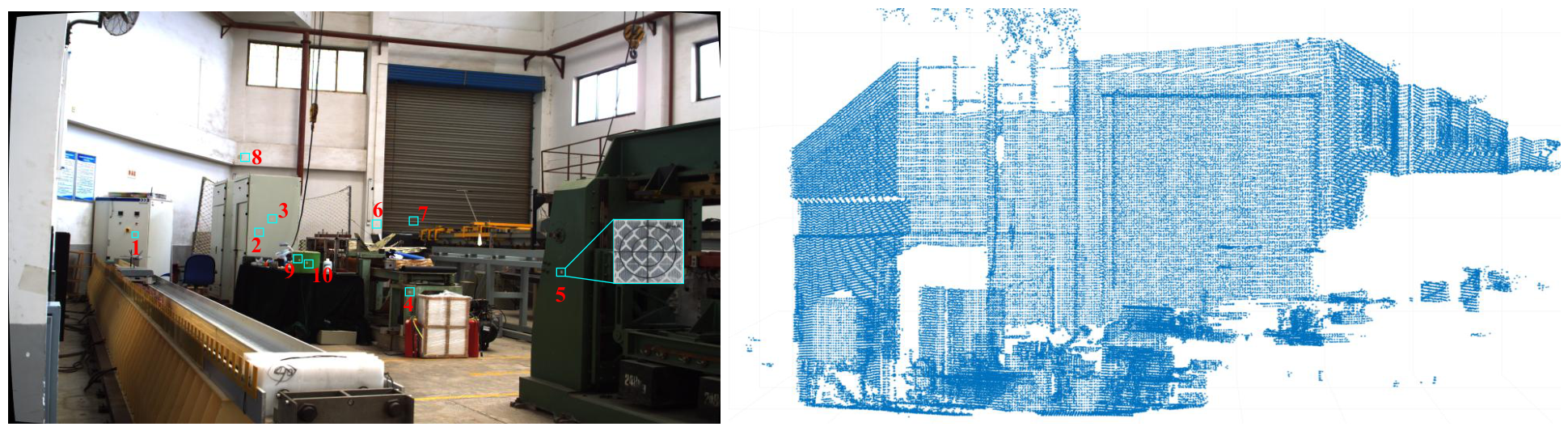
The measurement point distribution and experimental scene are illustrated in Figure 12. The spatial coordinates of the measurement points in the total station coordinate system are listed in Table 1, respectively. The experiments were conducted in an industrial equipment storage environment. As shown in Table 2, Table 3, Table 4 and Table 5, the proposed method achieves significantly higher measurement accuracy than the nearest-neighbor and interpolation-based methods.

Figure 12. Measurement Point Distribution and Experimental Scene.

Table 1. Spatial Coordinates of Measurement Points in the Total Station Coordinate System (Ground Truth).

No.	X/m	Y/m	Z/m	Distance/m
1	14.2560	0.4400	−0.4279	NaN
2	11.5028	2.0273	−0.3248	3.1796
3	11.5072	2.2223	−0.0985	3.2956
4	7.2007	2.5700	−0.9722	7.3899
5	4.4608	2.4115	−0.6192	9.9935
6	18.8292	6.9704	0.1205	7.9913
7	19.2355	8.2427	0.2688	9.2823
8	19.5384	3.3936	1.8483	6.4659
9	8.2742	1.7133	−0.6796	6.1209
10	8.2337	1.7872	−0.7094	6.1776

Table 2. Measurement Results of the Proposed Method.

No.	Type	X/m	Y/m	Z/m	Distance/m	Error/m
1	Mul_Plane	−5.0807	0.2524	12.9955	NaN	NaN
2	Mul_Plane	−2.4681	0.1693	11.1873	3.1784	−0.0012
3	Plane	−2.2891	−0.0458	11.2864	3.2868	−0.0088
4	Mass	−0.1072	0.7836	7.5716	7.3781	−0.0118
5	Mul_Plane	0.9704	0.3690	5.0069	10.0224	0.0289
6	Mul_Plane	−1.1872	0.0703	19.9802	7.9987	0.0074
7	Mul_Plane	−0.1741	−0.0215	20.9438	9.3448	0.0625
8	Mul_Plane	−4.7152	−1.8256	19.1249	6.4824	0.0165
9	Curve	−1.3505	0.4581	8.1756	6.0982	0.0227
10	Curve	−1.2699	0.4905	8.1652	6.1572	−0.0204

Table 3. Nearest-Neighbor Measurement Results.

No.	X/m	Y/m	Z/m	Distance/m	Error/m
1	−5.0842	0.2468	13.0037	NaN	NaN
2	−2.4726	0.1634	11.1742	3.2051	0.0255
3	−2.2978	−0.0541	11.2639	3.3387	0.0431
4	−0.1198	0.7687	7.5482	7.4762	0.0863
5	0.9362	0.3418	4.9726	10.1683	0.1748
6	−1.2115	0.0479	19.9274	8.0585	0.0672
7	−0.2086	−0.0548	20.8923	9.4526	0.1703
8	−4.7562	−1.8624	19.0741	6.5397	0.0738
9	−1.3811	0.4246	8.1292	6.1504	0.0295
10	−1.3038	0.4553	8.1178	6.2145	0.0369

Table 4. Interpolation-Based Measurement Results.

No.	X/m	Y/m	Z/m	Distance/m	Error/m
1	−5.0927	0.2419	13.0096	NaN	NaN
2	−2.4854	0.1583	11.1749	3.1917	0.0131
3	−2.3112	−0.0628	11.2864	3.3083	0.0242
4	−0.1308	0.7675	7.5521	7.4068	0.0283
5	0.9528	0.3521	4.9876	10.0537	0.0597
6	−1.2064	0.0537	19.9586	8.0178	0.0283
7	−0.1942	−0.0382	20.9218	9.3763	0.0764
8	−4.7338	−1.8414	19.1042	6.5012	0.0298
9	−1.3665	0.4421	8.1572	6.1173	0.0059
10	−1.2858	0.4739	8.1468	6.1776	0.0125

Table 5. Error Comparison.

Method	Mean/m	RMSE/m	Std/m	SSE/m2
Nearest Neighbor	0.0563	0.0712	0.0589	0.05068
Interpolation	0.0346	0.0412	0.0351	0.01698
Our method	0.0181	0.0218	0.0227	0.00476

4.3. Accuracy Stability Experiment Under Sparse Point Cloud Density

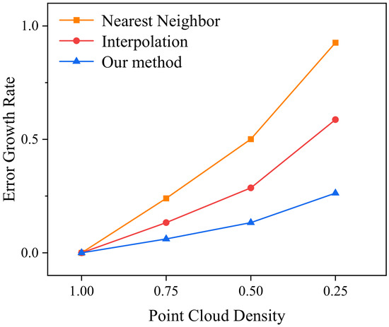
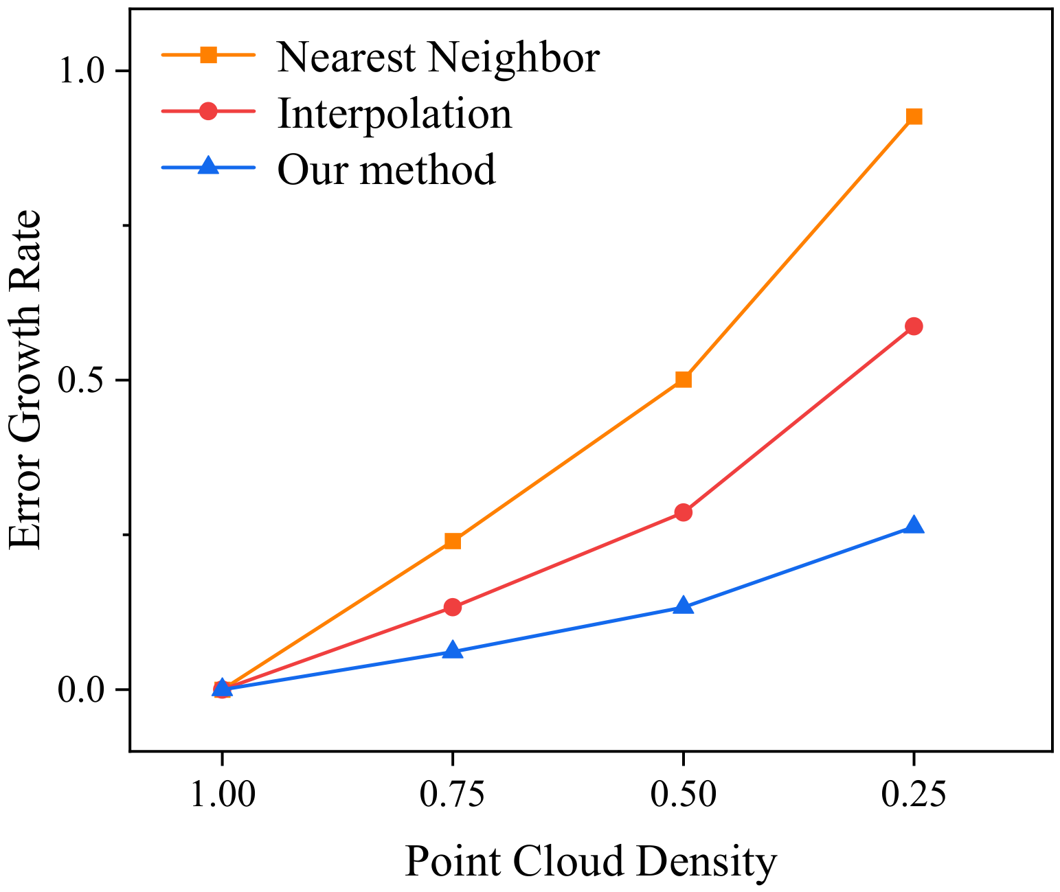
To further evaluate the applicability and robustness of the proposed method under sparse point cloud conditions, an accuracy stability experiment was conducted under different point cloud densities. In the experiment, the original LiDAR point cloud was randomly downsampled to generate measurement data with different density levels. Three density conditions, corresponding to 75%, 50%, and 25% of the original point cloud density, were considered, as illustrated in Figure 13. The nearest-neighbor method, interpolation-based method, and the proposed method were then employed to estimate the spatial coordinates corresponding to image measurement points. Using the total station measurements as ground truth, the measurement errors under different point cloud densities were quantitatively compared to evaluate the accuracy preservation capability of each method under sparse sampling conditions. The relative distances and corresponding errors with respect to No. 1 under different point cloud densities are listed in Table 6, Table 7, Table 8 and Table 9, while the error growth rates are illustrated in Figure 14. The experimental results show that the proposed method achieves the lowest measurement error and the highest accuracy under all density conditions. Meanwhile, compared with the nearest-neighbor and interpolation-based methods, the proposed method exhibits the slowest error growth as the point cloud density decreases, demonstrating superior robustness under sparse point cloud conditions.

Figure 13. Experimental Scene Point Clouds at Varying Densities (100–25%).

Table 6. Measurement Results Under 75% Point Cloud Density.

No.	Distance/m			Error/m
	Nearest Neighbor	Interpolation	Our Method	Nearest Neighbor	Interpolation	Our Method
1	NaN	NaN	NaN	NaN	NaN	NaN
2	3.2093	3.1948	3.1779	0.0297	0.0152	−0.0017
3	3.3442	3.3119	3.2858	0.0486	0.0163	−0.0098
4	7.4847	7.4123	7.3767	0.0948	0.0224	−0.0132
5	10.1768	10.0602	10.0238	0.1833	0.0667	0.0303
6	8.0661	8.0227	7.9993	0.0748	0.0314	0.0080
7	9.4629	9.3826	9.3462	0.1806	0.1003	0.0639
8	6.5482	6.5063	6.4832	0.0823	0.0404	0.0173
9	6.1567	6.1193	6.0968	0.0358	−0.0016	−0.0241
10	6.2213	6.1794	6.1559	0.0437	0.0018	−0.0217

Table 7. Measurement Results Under 50% Point Cloud Density.

No.	Distance/m			Error/m
	Nearest Neighbor	Interpolation	Our Method	Nearest Neighbor	Interpolation	Our Method
1	NaN	NaN	NaN	NaN	NaN	NaN
2	3.2142	3.1983	3.1773	0.0346	0.0187	−0.0023
3	3.3517	3.3159	3.2848	0.0561	0.0203	−0.0108
4	7.4948	7.4183	7.3756	0.1049	0.0284	−0.0143
5	10.1862	10.0683	10.0248	0.1927	0.0748	0.0313
6	8.0752	8.0278	8.0008	0.0839	0.0365	0.0095
7	9.4748	9.3896	9.3481	0.1925	0.1073	0.0658
8	6.5583	6.5113	6.4842	0.0924	0.0454	0.0183
9	6.1637	6.1208	6.0957	0.0428	−0.0001	−0.0252
10	6.2282	6.1812	6.1547	0.0506	0.0036	−0.0229

Table 8. Measurement Results Under 25% Point Cloud Density.

No.	Distance/m			Error/m
	Nearest Neighbor	Interpolation	Our Method	Nearest Neighbor	Interpolation	Our Method
1	NaN	NaN	NaN	NaN	NaN	NaN
2	3.2219	3.2037	3.1768	0.0423	0.0241	−0.0028
3	3.3608	3.3229	3.2837	0.0652	0.0273	−0.0119
4	7.5089	7.4269	7.3742	0.1190	0.0370	−0.0157
5	10.2028	10.0803	10.0263	0.2093	0.0868	0.0328
6	8.0889	8.0363	8.0023	0.0976	0.0450	0.0110
7	9.4928	9.4024	9.3519	0.2105	0.1201	0.0696
8	6.5728	6.5183	6.4863	0.1069	0.0524	0.0204
9	6.1729	6.1237	6.0942	0.0520	0.0028	−0.0267
10	6.2389	6.1839	6.1532	0.0613	0.0063	−0.0244

Table 9. Error Comparison Under Different Point Cloud Densities (Bold values indicate the best results).

Method	Density	Mean/m	RMSE/m	Std/m	SSE/m2
Nearest Neighbor	100%	0.0563	0.0712	0.0589	0.0507
	75%	0.0698	0.0882	0.0731	0.0778
	50%	0.0845	0.1068	0.0884	0.1141
	25%	0.1085	0.1286	0.1193	0.1486
Interpolation	100%	0.0346	0.0412	0.0351	0.0170
	75%	0.0392	0.0468	0.0398	0.0196
	50%	0.0445	0.0531	0.0451	0.0282
	25%	0.0549	0.0675	0.0592	0.0411
Our method	100%	0.0181	0.0218	0.0227	0.0048
	75%	0.0192	0.0231	0.0197	0.0053
	50%	0.0205	0.0247	0.0210	0.0061
	25%	0.0229	0.0288	0.0245	0.0075

Figure 14. Comparison of Error Growth under Different Point Cloud Densities.

The error growth rate is used to describe the relative increase in measurement error compared with the original point cloud density, which reflects the robustness of different methods under sparse point cloud conditions. For the nearest-neighbor method, when the point cloud density decreased to 75% of the original point cloud, the mean absolute error (Mean) increased from 0.0563 m to 0.0698 m, corresponding to an error growth rate of 24.0%. Under the 25% density condition, the Mean reached 0.1085 m, corresponding to a significant growth rate of 92.6%. For the interpolation-based method, the Mean increased from 0.0346 m to 0.0392 m at 75% density, corresponding to an error growth rate of 13.3%. When the density decreased to 25%, the Mean further increased to 0.0549 m, corresponding to a growth rate of 58.7%. In contrast, the proposed method exhibited significantly better robustness under sparse point cloud conditions. At 75% density, the Mean increased only from 0.0181 m to 0.0192 m, corresponding to an error growth rate of 6.1% Even under the extremely sparse 25% density condition, the Mean increased only to 0.0229 m, corresponding to a growth rate of 26.5%. These results demonstrate that the proposed method achieves substantially better measurement stability under sparse point cloud conditions compared with the nearest-neighbor and interpolation-based methods.

4.4. Accuracy Comparison of Different Geometric Measurement Strategies

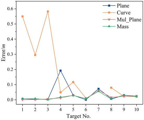
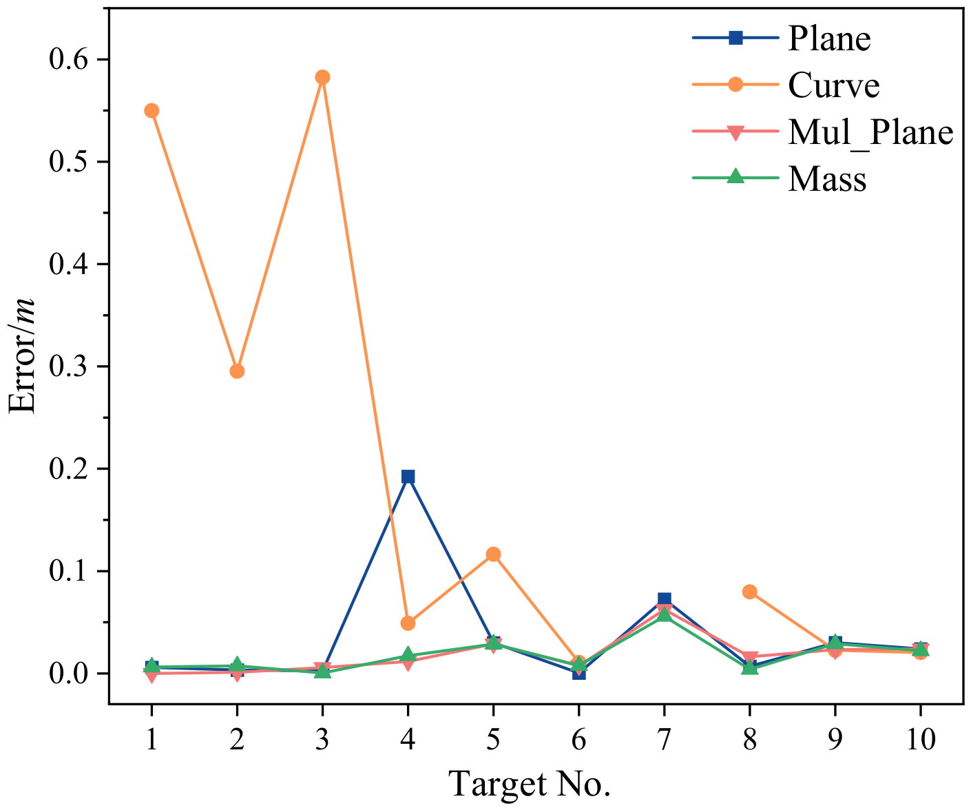
To validate the effectiveness of the proposed adaptive measurement strategies for different target surfaces and to analyze the influence of different local surface fitting methods on measurement accuracy, four geometric measurement strategies were separately applied to measure 10 marked points. In the experiment, the relative distances between each marked point and Point No. 1 measured by the total station were regarded as ground truth. Considering that the geometric feature analysis in the previous section indicates that the measured targets are more likely to exhibit multi-plane structures, the three-dimensional coordinate of Point No. 1 obtained by the Mul_Plane measurement strategy was selected as the reference point. Each method measured the 10 marked points three times, and the average values were used as the final measurement results. The experimental results are listed in Table 10, while the corresponding error distributions are illustrated in Figure 15. The results demonstrate that employing the corresponding adaptive measurement strategy for different target types can effectively achieve lower measurement errors and higher measurement accuracy.

Table 10. ErrorComparison of Different Geometric Measurement Strategies.

Method	No.	X/m	Y/m	Z/m	Distance/m	Error/m
Plane	1	−5.0786	0.2523	12.9899	0.0060	0.0060
	2	−2.4667	0.1692	11.1812	3.1830	0.0034
	3	−2.2882	−0.0458	11.2819	3.2900	0.0026
	4	−0.1034	0.7553	7.2977	7.5824	0.1925
	5	0.9701	0.3689	5.0053	10.0235	0.0299
	6	−1.1867	0.0702	19.9721	7.9918	0.0005
	7	−0.1742	−0.0215	20.9557	9.3549	0.0725
	8	−4.7128	−1.8246	19.1151	6.4729	0.0069
	9	−1.3519	0.4586	8.1838	6.0909	0.0301
	10	−1.2705	0.4907	8.1692	6.1537	0.0239
Curve	1	−4.8805	0.2425	12.4834	0.5499	0.5499
	2	−2.3840	0.1635	10.8060	3.4748	0.2952
	3	−2.1298	−0.0426	10.5011	3.8752	0.5826
	4	−0.1080	0.7889	7.6222	7.3408	0.0490
	5	0.9455	0.3596	4.8786	10.1100	0.1165
	6	−1.1859	0.0702	19.9588	7.9806	0.0107
	7	No solution
	8	−4.6905	−1.8160	19.0249	6.3863	0.0797
	9	−1.3505	0.4581	8.1756	6.0982	0.0227
	10	−1.2699	0.4905	8.1652	6.1572	0.0204
Mul_Plane	1	−5.0807	0.2524	12.9955	0.0000	0.0000
	2	−2.4681	0.1693	11.1873	3.1784	0.0012
	3	−2.2891	−0.0458	11.2864	3.2868	0.0057
	4	−0.1072	0.7836	7.5716	7.3781	0.0118
	5	0.9704	0.3690	5.0069	10.0224	0.0289
	6	−1.1872	0.0703	19.9802	7.9987	0.0074
	7	−0.1741	−0.0215	20.9438	9.3448	0.0624
	8	−4.7152	−1.8256	19.1249	6.4824	0.0164
	9	−1.3506	0.4581	8.1762	6.0977	0.0233
	10	−1.2705	0.4907	8.1693	6.1536	0.0240
Mass	1	−5.0785	0.2523	12.9896	0.0063	0.0063
	2	−2.4667	0.1692	11.1812	3.1870	0.0074
	3	−2.2875	−0.0458	11.2787	3.2922	0.0004
	4	−0.1073	0.7844	7.5791	7.3726	0.0173
	5	0.9705	0.3690	5.0071	10.0222	0.0288
	6	−1.18612	0.0702	19.9622	7.9835	0.0078
	7	−0.1741	−0.0215	20.9360	9.3382	0.0558
	8	−4.7099	−1.8235	19.1036	6.4619	0.0041
	9	−1.3517	0.4585	8.1827	6.0919	0.0291
	10	−1.2702	0.4906	8.1672	6.1554	0.0222

Figure 15. Error Line Plot of the Four Measurement Strategies.

4.5. Comparison Between the Adaptive and Fixed Mass Strategies Under Different Point-Cloud Densities

As shown in Figure 15, at the original point-cloud density, the fixed Mass strategy achieved measurement accuracy comparable to that of the adaptive measurement method. To further evaluate the measurement robustness of the fixed Mass strategy under different point-cloud densities, the original point cloud was downsampled to 75%, 50%, and 25% of its original density, respectively, and the fixed Mass strategy was compared with the adaptive measurement method. The measurement points described in Section 4.2 were used as the experimental targets, and the results are presented in Table 11.

Table 11. Measurement Results of the Adaptive Method and Fixed Mass Strategy under Different Point Cloud Densities.

Method	Density	Mean/m	RMSE/m	Std/m	SSE/m2
Fixed Mass	100%	0.0180	0.0268	0.0256	0.00718
	75%	0.0319	0.0404	0.0372	0.01632
	50%	0.0376	0.0462	0.0429	0.02134
	25%	0.0437	0.0528	0.0498	0.02787
Adaptive	100%	0.0181	0.0218	0.0227	0.00476
	75%	0.0192	0.0231	0.0197	0.0053
	50%	0.0205	0.0247	0.0210	0.0061
	25%	0.0229	0.0288	0.0245	0.0075

At the original point cloud density, the mean measurement errors of the fixed Mass strategy and the adaptive method were $1.80\mathrm{cm}$ and $1.81\mathrm{cm}$, respectively, indicating comparable measurement performance. This result is consistent with that shown in Figure 15. When the local point cloud is relatively complete, the Mass strategy can select stable representative points from different spatial directions, and the resulting bilinear patch can approximate different types of local surfaces to a certain extent. As the point-cloud density decreased, the measurement errors of both methods increased, but the error of the fixed Mass strategy increased more rapidly. When the point-cloud density was reduced to 25% of the original density, the mean measurement error of the adaptive method was $2.29\mathrm{cm}$, corresponding to an error growth rate of 26.5%. In contrast, the mean measurement error of the fixed Mass strategy increased to $4.37\mathrm{cm}$, corresponding to an error growth rate of 142.8%. These results indicate that the fixed Mass strategy is less robust under sparse point cloud conditions.

4.6. Cross-Scene Generalization Performance Analysis

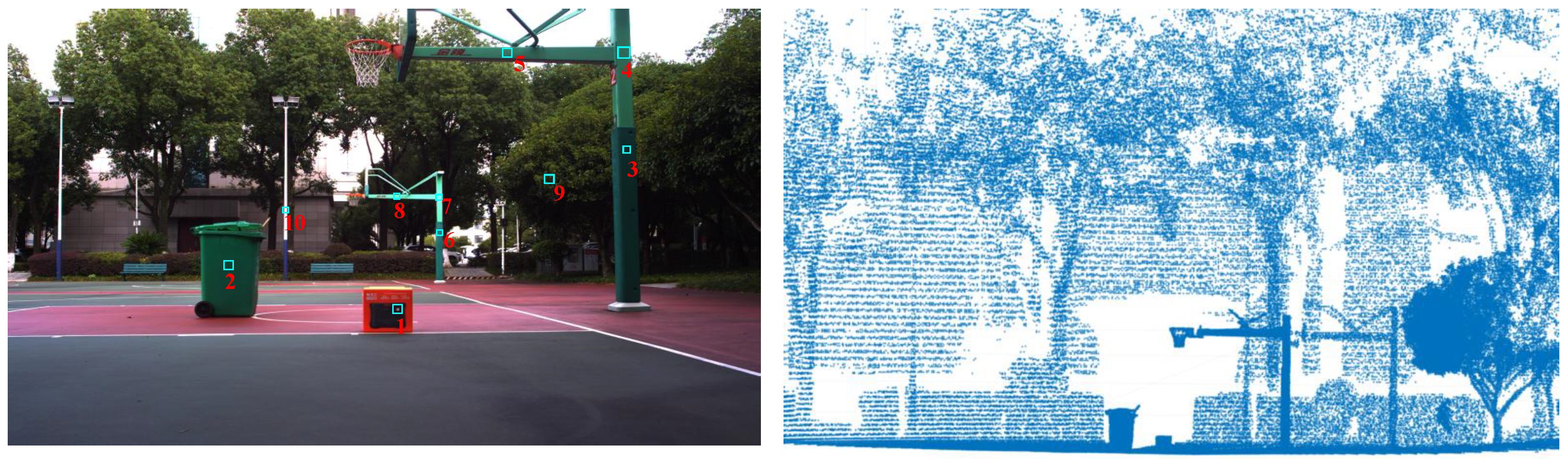
To further evaluate the cross-scene generalization capability of the proposed method, an additional outdoor experiment was conducted using the same LiDAR–camera extrinsic calibration parameters and classification thresholds as in the indoor experiment. The experimental scene and measurement-point distribution are shown in Figure 16. As shown in Table 12, Table 13, Table 14, Table 15 and Table 16, the proposed method achieved a mean absolute error of 3.14 cm in the outdoor scene, which was higher than the 1.81 cm obtained indoors but still lower than those of the nearest-neighbor back-projection method and the interpolation-based method, at 4.21 cm and 6.30 cm, respectively. These results demonstrate that the proposed method maintains its accuracy advantage across different scenes.

Figure 16. Outdoor Measurement Point Distribution and Experimental Scene.

Table 12. Spatial Coordinates of Measurement Points in the Outdoor Total Station Coordinate System (Ground Truth).

No.	X/m	Y/m	Z/m	Distance/m
1	6.0187	−0.4063	−0.6412	NaN
2	8.1065	0.9984	−0.4059	2.6154
3	8.2359	−3.1018	0.8886	3.5476
4	8.3326	−3.0845	1.9294	4.1552
5	8.4289	−1.6147	1.9318	4.0408
6	25.3294	−3.6482	−0.0188	19.9298
7	25.3427	−3.6916	0.9293	20.4246
8	25.4315	−2.2428	0.9105	19.6178
9	10.2624	−6.4973	1.9286	7.7762
10	34.2589	1.5276	0.7497	28.4756

Table 13. Measurement Results of the Proposed Method in Outdoor Scene.

No.	Type	X/m	Y/m	Z/m	Distance/m	Error/m
1	Mul_Plane	6.0195	−0.4067	−0.6423	NaN	NaN
2	Plane	8.1248	0.9816	−0.4249	2.6471	0.0317
3	Mul_Plane	8.2627	−3.0834	0.8728	3.5755	0.0279
4	Mul_Plane	8.3581	−3.0649	1.9154	4.1897	0.0345
5	Mul_Plane	8.4536	−1.5968	1.9173	4.0710	0.0302
6	Mul_Plane	25.3524	−3.6678	−0.0356	19.9629	0.0331
7	Mul_Plane	25.3669	−3.7121	0.9112	20.4514	0.0268
8	Mul_Plane	25.4553	−2.2624	0.8935	19.6547	0.0369
9	Mass	10.2858	−6.5162	1.9126	7.8067	0.0305
10	Curve	34.2829	1.5096	0.7319	28.5080	0.0324

Table 14. Nearest-Neighbor Measurement Results in Outdoor Scene.

No.	X/m	Y/m	Z/m	Distance/m	Error/m
1	6.0418	−0.4286	−0.6614	NaN	NaN
2	8.1516	0.9573	−0.4472	2.6777	0.0623
3	8.2924	−3.0584	0.8524	3.6124	0.0648
4	8.3931	−3.0427	1.8952	4.2167	0.0615
5	8.4879	−1.5722	1.8971	4.1047	0.0639
6	25.3856	−3.6985	−0.0649	19.9927	0.0629
7	25.4003	−3.7449	0.8857	20.4889	0.0643
8	25.4897	−2.2969	0.8678	19.6796	0.0618
9	10.3192	−6.5483	1.8873	7.8397	0.0635
10	34.3214	1.4781	0.7056	28.5397	0.0641

Table 15. Interpolation-Based Measurement Results in Outdoor Scene.

No.	X/m	Y/m	Z/m	Distance/m	Error/m
1	6.0329	−0.4195	−0.6538	NaN	NaN
2	8.1386	0.9659	−0.4376	2.6563	0.0409
3	8.2754	−3.0697	0.8615	3.5911	0.0435
4	8.3742	−3.0531	1.9049	4.1965	0.0413
5	8.4709	−1.5837	1.9072	4.0836	0.0428
6	25.3684	−3.6819	−0.0513	19.9695	0.0397
7	25.3827	−3.7256	0.8986	20.4698	0.0452
8	25.4718	−2.2789	0.8819	19.6597	0.0419
9	10.3011	−6.5308	1.9004	7.8193	0.0431
10	34.3005	1.4954	0.7192	28.5181	0.0425

Table 16. Error Comparison in Outdoor Scene.

Method	Mean/m	RMSE/m	Std/m	SSE/m2
Nearest Neighbor	0.0630	0.0798	0.0735	0.0573
Interpolation	0.0421	0.0528	0.0482	0.02508
Our method	0.0314	0.0415	0.0378	0.0155

4.7. Sensitivity Analysis of Geometric Classification Thresholds

The proposed adaptive surface selection strategy relies on three geometric thresholds, including the curvature threshold $T_{\kappa }$, the normal entropy threshold $T_H$, and the normal deviation threshold $T_{std}$. Since these thresholds directly affect the classification of local surface geometry, their sensitivity was analyzed to evaluate the robustness of the proposed geometric classification strategy.

In the sensitivity analysis, one threshold was varied while the other two thresholds were fixed to their default values ($T_{\kappa }=0.1$, $T_H=2.5$, and $T_{std}=70°$). The curvature threshold was tested within the range of 0.05–0.15, the normal entropy threshold was varied from 2.0 to 3.0, and the normal deviation threshold was changed from 60° to 80°. The classification results under different parameter settings were compared with the results obtained using the default thresholds. The overall stability of each threshold is summarized in Table 17.

Table 17. Summary of Sensitivity Analysis for Geometric Classification Thresholds.

Parameter	Tested Range	Stable Classification	Changed Classification
$T_{\kappa }$	0.05–0.15	73.0%	27.0%
$T_H$	2.0–3.0	66.7%	33.3%
$T_{std}$	60°–80°	75.0%	25.0%

As shown in Table 17, moderate variations of the three geometric thresholds only cause limited changes in surface classification. The curvature threshold $T_{\kappa }$ has a relatively larger influence because curvature directly reflects local geometric variation and affects the discrimination between planar, curved, and multi-plane structures. However, most measurement regions remain consistently classified within the tested range.

The normal entropy threshold $T_H$ and normal deviation threshold $T_{std}$ exhibit higher stability. The classification changes mainly occur in geometrically ambiguous regions, where local structures contain transitional characteristics between two surface categories. For example, irregular boundaries or partially curved surfaces may be classified differently when the thresholds approach their extreme values.

Overall, the sensitivity analysis demonstrates that the proposed geometry-guided classification strategy is not highly dependent on a specific threshold combination. The default parameters provide stable surface recognition performance, while moderate threshold variations only influence a limited number of ambiguous regions. Therefore, the proposed adaptive model selection framework can maintain reliable geometric classification without strict threshold tuning.

5. Discussion

This paper proposes an adaptive measurement method based on surface geometric characteristics to address the accuracy degradation and poor adaptability of LiDAR-camera fusion measurement under sparse point clouds and complex target geometries. Unlike conventional methods based on discrete point-to-pixel correspondence or fixed geometric assumptions, the proposed method establishes a geometric intersection framework between viewing rays and continuous surface models. By classifying local surfaces into plane, curve, multi-plane, and scattered structures, appropriate geometric models are adaptively selected to improve measurement reliability under diverse geometric conditions.

Experimental results demonstrate that the proposed method improves the average LiDAR measurement accuracy from 5.63 cm obtained by the nearest-neighbor search method to 1.81 cm. Furthermore, under sparse point cloud conditions, the proposed method maintains better robustness than conventional methods. When the point cloud density decreases to 25% of the original density, the mean absolute error increases by only 26.5%, which is significantly lower than the error growth of the nearest-neighbor method (92.6%) and the interpolation-based method (58.7%). These results indicate that the proposed adaptive surface reconstruction and ray-surface intersection strategy can effectively reduce the influence of point cloud sparsity on measurement accuracy.

At the original point-cloud density, the fixed Mass strategy and the adaptive method achieve comparable mean errors of 1.80 cm and 1.81 cm, respectively, indicating that the Mass model can provide an effective local surface approximation when sufficient point-cloud information is available. However, when the point-cloud density decreases to 25%, the mean error of the fixed Mass strategy increases to 4.37 cm, corresponding to an error growth rate of 142.8%, whereas the adaptive method maintains a mean error of 2.29 cm, with an error growth rate of only 26.5%. By selecting an appropriate surface model according to the identified local geometric characteristics, the adaptive method preserves high measurement accuracy while maintaining strong robustness as the point-cloud density decreases. Therefore, rather than providing a substantial accuracy improvement for every geometric category at the original point-cloud density, the adaptive strategy achieves the best overall performance by balancing measurement accuracy and robustness across the evaluated point-cloud densities.

It should be noted that this study mainly evaluates measurement performance using relative distance error rather than absolute 3D coordinate error. This choice is consistent with industrial equipment measurement and collision prevention applications, where relative spatial relationships are often more important than absolute positions in a global coordinate system. However, relative distance error cannot fully represent global localization accuracy, which is also affected by coordinate registration and calibration uncertainties. A comprehensive evaluation of absolute 3D coordinate accuracy considering total station uncertainty and LiDAR-camera calibration errors will be investigated in future work. Future work will focus on adaptive parameter optimization, extension to dynamic measurement scenarios, and multi-sensor fusion to further improve measurement robustness under complex environments.

References

- Wang, Z.; Liu, Y.; Wang, X.; Zhang, D.; Qin, L.; Liu, J.; Li, M.; Liu, J. Field Calibration Method for Industrial Robots Based on Single Position Sensitive Device. IEEE Trans. Instrum. Meas. 2023, 72, 1–12. [Google Scholar] [CrossRef] [Scilit]
- Zhou, B.; Zhao, L.; Zhang, T.; Zhao, J.; Xia, R.; Liu, D. Aviation equipment measurement and assembly analysis method based on robotic system. Measurement 2024, 234, 114810. [Google Scholar] [CrossRef] [Scilit]
- Tang, G.; Gu, J.; Zhu, W.; Claramunt, C.; Zhou, P. HD Camera-Equipped UAV Trajectory Planning for Gantry Crane Inspection. Remote Sens. 2022, 14, 1658. [Google Scholar] [CrossRef] [Scilit]
- Ali, A.H.; Zayed, T.; Wang, R.D.; Kit, M.Y.S. Tower crane safety technologies: A synthesis of academic research and industry insights. Autom. Constr. 2024, 163, 105429. [Google Scholar] [CrossRef] [Scilit]
- Meng, W.; Cheng, L.; Liu, Y.; Zheng, W.; Tan, P.; Guo, F. Shaking table test of a novel slope-type sliding pendulum isolation system for seismic protection of electrical equipment. Soil Dyn. Earthq. Eng. 2026, 208, 110365. [Google Scholar] [CrossRef] [Scilit]
- Gaspar, J.; Soares, A.C.; Martins, R.F. Analysis and prevention of wear failure in a hammer crusher used in a cement plant production line. Eng. Fail. Anal. 2025, 182, 110009. [Google Scholar] [CrossRef] [Scilit]
- Liu, X.; Liu, J.; Liu, B.; Qu, Y.; Zhu, Z.; Zhao, Z. A 6-DOF calibration method for pose measurement equipment based on parallel mechanism trajectories. Meas. Sci. Technol. 2026, 36, 125011. [Google Scholar] [CrossRef] [Scilit]
- Chen, Z.; Yuan, Y.; Liu, Z.; Li, H. Monitoring of Surrounding Rock Deformation in Underground Roadways Using 3D Laser Scanning and Analysis of Environmental Influencing Factors. Remote Sens. 2026, 18, 1279. [Google Scholar] [CrossRef] [Scilit]
- Kang, S.; Kim, S.; Kim, G.H. Integration of real-time labor positioning data and 3D laser scan model for dangerous zone access monitoring. J. Build. Eng. 2025, 111, 113445. [Google Scholar] [CrossRef] [Scilit]
- Cao, B.; Yu, Z.; Li, M.; Zhang, C.; Xu, B. A novel method for enhanced ultra-wideband positioning accuracy in GPS-denied environments. Adv. Eng. Inform. 2026, 74, 104767. [Google Scholar] [CrossRef] [Scilit]
- Gong, B.; Wang, Y.; Lin, C.; Liu, H. Roadside LiDAR-Camera Fusion Detection Based on Spatiotemporal Calibration. IEEE Sens. J. 2025, 25, 31313–31325. [Google Scholar] [CrossRef] [Scilit]
- Ni, J.; Gao, B.; Zhu, H.; Zhao, M.; Liu, X. Visual Localization Algorithm with Dynamic Point Removal Based on Multi-Modal Information Association. ISPRS Int. J. Geo-Inf. 2026, 15, 60. [Google Scholar] [CrossRef] [Scilit]
- Chen, X.; Song, Z.; Zhou, J.; Xie, D.; Lu, J. Camera and LiDAR Fusion for Urban Scene Reconstruction and Novel View Synthesis via Voxel-Based Neural Radiance Fields. Remote Sens. 2023, 15, 4628. [Google Scholar] [CrossRef] [Scilit]
- Qiu, Z.; Shao, J.; Xiao, Z.; Yin, X.; Wang, L. SAVF-net: Sparse attention and multi-scale voxel fusion network for high-accuracy 3D measurement with LiDAR point clouds. Meas. Sci. Technol. 2026, 37, 085204. [Google Scholar] [CrossRef] [Scilit]
- Zhang, S.J.; Chiang, P.J. Enhanced association and detection accuracy in multi-object tracking with camera-LiDAR Data Fusion. Opt. Lasers Eng. 2025, 194, 109125. [Google Scholar] [CrossRef] [Scilit]
- Yu, Y.; Fan, S.; Li, L.; Wang, T.; Li, L. Automatic Targetless Monocular Camera and LiDAR External Parameter Calibration Method for Mobile Robots. Remote Sens. 2023, 15, 5560. [Google Scholar] [CrossRef] [Scilit]
- Yi, H.; Liu, B.; Zhao, B.; Liu, E. Extrinsic Calibration for LiDAR–Camera Systems Using Direct 3D–2D Correspondences. Remote Sens. 2022, 14, 6082. [Google Scholar] [CrossRef] [Scilit]
- Xi, H.; Zhang, S.; Dong, Q.; Tong, Y.; Wu, S.; Yuan, J.; Zhang, X. R-VoxelMap: Accurate Voxel Mapping with Recursive Plane Fitting for Online LiDAR Odometry. IEEE Robot. Autom. Lett. 2026, 11, 2402–2409. [Google Scholar] [CrossRef] [Scilit]
- Xia, J.; Ma, S.; Luan, G.; Dong, P.; Geng, R.; Zou, F.; Yin, J.; Zhao, Z. An Improved Method for Single Tree Trunk Extraction Based on LiDAR Data. Remote Sens. 2025, 17, 1271. [Google Scholar] [CrossRef] [Scilit]
- Zhang, J.; Guo, Q.; Jin, S.; Pang, L.; Yang, F.; Bi, H. L1/2-Norm Regularization Outlier Removal and Moving Least Squares-Based TomoSAR Point Cloud Optimization of Mountain Areas. IEEE Geosci. Remote Sens. Lett. 2025, 22, 1–5. [Google Scholar] [CrossRef] [Scilit]
- Wang, H.; Xu, J.; Luo, X.; Zhang, T.; Chen, X.; Duan, R.; Liu, Y.; Zheng, J.; Hong, W.; Ji, X.; et al. mmE-Loc: Facilitating Accurate Drone Landing with Ultra-High-Frequency Localization. IEEE Trans. Mob. Comput. 2026, 25, 10651–10669. [Google Scholar] [CrossRef] [Scilit]
- Zhao, L.; Hu, Y.; Han, F.; Dou, Z.; Li, S.; Zhang, Y.; Wu, Q. Multi-sensor missile-borne LiDAR point cloud data augmentation based on Monte Carlo distortion simulation. CAAI Trans. Intell. Technol. 2025, 10, 300–316. [Google Scholar] [CrossRef] [Scilit]
- Liu, W.; Gao, F.; Cai, Y.; Zhang, L.; Liu, Y.; Fu, H.; Chen, C.; Deng, F. Outdoor full-range geolocator with multi-vision fusion and self-supervised truncation filtering. Sci. China (Inf. Sci.) 2026, 69, 505–506. [Google Scholar] [CrossRef] [Scilit]
- Zhang, W.; Zhao, J.; Chen, M.; Chen, Y.; Yan, K.; Li, L.; Qi, J.; Wang, X.; Luo, J.; Chu, Q. Registration of optical imagery and LiDAR data using an inherent geometrical constraint. Opt. Express 2015, 23, 7694–7702. [Google Scholar] [CrossRef] [Scilit]
- Zhou, Z.; Jiang, W.; Guo, C.; Liu, Y.; Zhou, X. A Lightweight LiDAR–Visual Odometry Based on Centroid Distance in a Similar Indoor Environment. Remote Sens. 2025, 17, 2850. [Google Scholar] [CrossRef] [Scilit]
- Zhao, X.; Wang, T.; Li, Y.; Zhang, B.; Liu, K.; Liu, D.; Wang, C.; Snoussi, H. Target-Driven Visual Navigation by Using Causal Intervention. IEEE Trans. Intell. Veh. 2024, 9, 1294–1304. [Google Scholar] [CrossRef] [Scilit]
- Luo, J.; Cui, W.; Shen, X. A Two-Step 3D LiDAR-Camera Calibration Method Using AR Tags. In Proceedings of the Proceedings Chinese Intelligent Systems Conference; Springer: Berlin/Heidelberg, Germany, 2022; pp. 443–452. [Google Scholar]
- Jaritz, M.; Charette, R.D.; Wirbel, E.; Perrotton, X.; Nashashibi, F. Sparse and Dense Data with CNNs: Depth Completion and Semantic Segmentation. In Proceedings of the 2018 International Conference on 3D Vision (3DV), Verona, Italy, 5–8 September 2018; pp. 52–60. [Google Scholar] [CrossRef] [Scilit]
- Uhrig, J.; Schneider, N.; Schneider, L.; Franke, U.; Brox, T.; Geiger, A. Sparsity Invariant CNNs. In Proceedings of the 2017 International Conference on 3D Vision (3DV), Qingdao, China, 10–12 October 2017; pp. 11–20. [Google Scholar] [CrossRef] [Scilit]
- Amiri-Simkooei, A.; Esmaeili, F.; Lindenbergh, R. Least squares B-spline approximation with applications to geospatial point clouds. Measurement 2025, 248, 116887. [Google Scholar] [CrossRef] [Scilit]
- Li, Z.; Zhong, M.; Wang, J.; Yuan, B.; Fan, K.; Tan, J.W. MonoDGD: Multi-scale depth-guided fusion for monocular 3D object detection. Meas. Sci. Technol. 2026, 37, 136001. [Google Scholar] [CrossRef] [Scilit]
- Liu, C.; Zhang, G.; Rong, Y.; Shao, W.; Meng, J.; Li, G.; Huang, Y. Hybrid metric-feature mapping based on camera and Lidar sensor fusion. Measurement 2023, 207, 112411. [Google Scholar] [CrossRef] [Scilit]
- Hartley, R.; Zisserman, A. Multiple View Geometry in Computer Vision; Cambridge University Press: Cambridge, UK, 2003; Volume 2. [Google Scholar]
- Mildenhall, B.; Srinivasan, P.P.; Tancik, M.; Barron, J.T.; Ramamoorthi, R.; Ng, R. NeRF: Representing Scenes as Neural Radiance Fields for View Synthesis. In Proceedings of the ECCV 2020; Springer: Cham, Switzerland, 2020; pp. 405–421. [Google Scholar]
- Wang, P.; Liu, L.; Liu, Y.; Theobalt, C.; Komura, T.; Wang, W. NeuS: Learning Neural Implicit Surfaces by Volume Rendering for Multi-view Reconstruction. In Proceedings of the NIPS’21: 35th International Conference on Neural Information Processing Systems, Online, 6–14 December 2021. [Google Scholar]
- Edelsbrunner, H.; Mucke, E.P. Three-dimensional alpha shapes. ACM Trans. Graph. 1994, 13, 43–72. [Google Scholar] [CrossRef] [Scilit]
- Chen, H.; Wu, J.; Huang, Z.; Xu, J.; Yin, Z.; Yao, Y. Automatic extrinsic calibration algorithm for LiDAR-camera fusion systems using spherical target. In Proceedings of the International Conference on Remote Sensing, Surveying, and Mapping (RSSM 2025); International Society for Optics and Photonics, SPIE: Xi’an, China, 2025; Volume 13642, p. 1364229. [Google Scholar] [CrossRef] [Scilit]
Disclaimer/Publisher’s Note: The statements, opinions and data contained in all publications are solely those of the individual author(s) and contributor(s) and not of MDPI and/or the editor(s). MDPI and/or the editor(s) disclaim responsibility for any injury to people or property resulting from any ideas, methods, instructions or products referred to in the content. |
© 2026 by the authors. Published by MDPI on behalf of the International Society for Photogrammetry and Remote Sensing. Licensee MDPI, Basel, Switzerland. This article is an open access article distributed under the terms and conditions of the Creative Commons Attribution (CC BY) license.