


Abstract
Leveraging larger-scale data with higher currency to incrementally update smaller-scale data, thereby upholding consistency across multiple scale databases, has become a core focus of contemporary map production tasks centered on data updates. Existing methods rely on rule-based constraints to extract change information and identify update-required objects, which have notable limitations in terms of method generalization and constraints on results. To address the above issues, we propose an intelligent incremental updating method for different scale building datasets supported by Categorical Boosting (CatBoost). The proposed method forms a general incremental updating framework for buildings through three steps: change information extraction, change information classification, and change information updating. Experiments conducted on different scale datasets from Ningbo, China, demonstrate that the proposed method can effectively identify update-required objects and generate more reasonable updated smaller-scale data than the comparative methods.
1. Introduction
Geospatial phenomena or entities manifest distinct spatial forms, structures, and details at different scales. To address the needs of spatial modeling and analysis at the macro, meso, and micro scales, researchers have abstracted the spatial morphological structures of various natural and human-induced phenomena on the Earth’s surface across multiple scales. This has resulted in the development of a series of topographic maps at diverse scales [1,2,3]. Against the backdrop of expanding geographic information application scenarios and accelerating urbanization, ensuring the timely update of multiple scale databases and the preservation of their consistency is a critical prerequisite for urban sustainable development. It also serves as the cornerstone for advancing high-cognitive geographic tasks such as dynamic management of digital cities and intelligent decision-making based on spatial reasoning [4,5]. Leveraging larger-scale data with higher currency to incrementally update smaller-scale data, thereby upholding consistency across multiple scale databases, has become a core focus of contemporary map production tasks centered on data updates [6]. However, multiple scale datasets are often collected independently and display substantial discrepancies [7,8]. Meanwhile, data update standards vary across scales: larger-scale data is usually directly derived from field surveys, remote sensing imagery, and other sources [9,10,11], featuring short update cycles and high efficiency. In contrast, maintaining the currency of smaller-scale data requiring cartographic generalization poses considerable challenges, which is typically achieved through the incremental update of larger-scale data.
The primary causes of graphic discrepancies among homonymous entities in different scale building datasets are twofold. The first is temporal changes: such graphic discrepancies primarily stem from geographic events (e.g., demolition or new construction) involving real-world building entities, which are not dynamically updated in smaller-scale building datasets. The second is representation-related changes: such discrepancies generally arise from inconsistent representational standards for the same geographic feature across databases of varying scales. The purpose of incremental updating is to rationally propagate graphic changes caused by temporal variations in larger-scale data to smaller-scale data, thereby minimizing inconsistencies in existing multiple scale datasets [12,13]. Theoretically, incremental updates should identify and update homonymous entities exhibiting temporal changes. Existing methods for incremental updating of change information primarily rely on rule-based reasoning method. This involves extracting graphic change information of homonymous entities and establishing a mapping relationship between graphic changes and update operations based on rule constraints [14,15]. However, existing multiple scale databases fail to fully comply with unified cartographic generalization rules. Even for data within the same region that share the same scale change degree, some areas may be over-generalized or under-generalized [16]. Using temporal changes and representation-related changes as classification criteria cannot directly guide incremental updates for multiple scale databases lacking unified standards. Therefore, to maintain consistency in multiple scale databases, graphic changes should be classified based on the degree of inconsistency among homonymous entities. Moreover, the inconsistency level of such entities not only associated with changes in their geometric features but also tied to the geometric characteristics of the change polygon. Establishing a universally effective evaluation system through rule-based constraints alone is challenging. More intelligent methods for modeling change information are needed to achieve efficient classification.
To address the above issues, we propose an intelligent incremental updating method for different scale building datasets supported by Categorical Boosting (CatBoost). This method employs matching combinations as the fundamental unit for building change detection, forming a universal incremental updating framework for buildings through three steps: change information extraction, change information classification, and change information updating.
The main contributions of this work can be summarized as follows:
- We systematically summarized and analyzed the graphical change characteristics of buildings across multiple scales and time phases, and adopted the inconsistency degree as the classification criterion for identifying objects requiring incremental updates. Meanwhile, we proposed a polygon aggregation algorithm based on Alpha-shape (termed Poly-Alpha) to aggregate homonymous building entities and extract polygons featuring inconsistent geometric variations, which can effectively filter out representation-related change of homonymous entities.
- Geometric features of homonymous entities and change polygons were extracted to characterize the degree of change in homonymous entities. A CatBoost classifier was introduced for detecting to-be-updated buildings, which can also enhance the interpretability of the classification process through the SHAP explanation model. Furthermore, we analyzed the distribution of SHAP feature values derived from the dataset to adjust hyperparameters reasonably, thereby boosting the generalization performance of the model.
- Guided by propagation update principles, we designed an incremental update method that takes matching groups as the fundamental unit for building change detection. This two-step workflow mitigates spatial conflicts and generates more geometrically reasonable updating outcomes.
2. Related Work
Maintaining the currency of spatial databases is a key focus in contemporary cartographic production. Its primary tasks include two core aspects: first, updating larger-scale vector data using multi-source data such as remote sensing imagery and trajectory data; second, updating smaller-scale data within multiple scale databases using high-currency larger-scale data.
The former has garnered significant attention in the remote sensing field, with research focusing on data extraction [17,18], change information extraction [19], and regularization based on remote sensing imagery [20,21]. In particular, a large number of advanced change detection methods for geospatial buildings have been proposed in recent years, which provide important technical support for building vector updating. Representative studies include high-precision building change detection frameworks based on remote sensing images [22,23,24], as well as novel deep learning-based change detection models for geographic objects [25,26]. These methods also show great potential in the updating of pre- and post-disaster building vector data, and relevant open datasets can be used for model validation and experimental verification [27,28]. Additionally, some scholars have leveraged multimodal models combined with remote sensing imagery to conduct research on updating historical vector data [29], which has further enhanced the currency of larger-scale data; however, in contrast, research on linkage-based updates between vector datasets remains relatively underdeveloped.
The latter concentrates on spatial entity matching [30,31], extraction and integration of update information [32,33], and detection and resolution of spatial conflicts [34]. Owing to the complexity of different scale data representation, the latter task has remained one of the core challenges in cartography.
Regarding the updating of different scale databases, commonly used methods primarily include reduction updating, cascade updating, and incremental updating [35]. The fundamental concept of reduction-based updating involves downscaling larger-scale maps using cartographic generalization rules and methods to generate a series of multiple scale databases. For example, Courtial et al. [36] employ a generative adversarial network (GAN) to produce a generalized map, and design a workflow of deep models (DeepMapScaler) [37] to achieve a step-by-step topographic map generalization. However, since map generalization is not yet fully automated, full-map generalization entails significant workload and suffers from low retrospective efficiency. A lot of issues remain to be addressed for real applications in map generalization utilizing artificial intelligence methods [38,39]. Cascade updates, however, build upon existing multiple scale databases by propagating updates to smaller-scale data through matching relationships. This approach primarily relies on event-driven updates: first, real-world events (e.g., demolition, new construction) trigger updates to larger-scale data; then, the update information is linked to corresponding entities in smaller-scale databases via matching relationships, and further propagated automatically to smaller-scale databases after cartographic generalization and spatial conflict resolution [40]. For instance, relevant studies have explored update propagation [41,42], conflict resolution [43,44], and the integration of map generalization events [45]. However, current multiple scale databases do not strictly adhere to unified cartographic generalization standards, rendering this relationship-driven data update method difficult to apply in complex multiple scale datasets. In contrast to the previous two approaches, incremental updating directly generates change information by comparing multiscale data, focusing research on the synthesis and database integration of this change information [46]. This method offers broader applicability since it does not require multiscale databases to strictly adhere to unified synthesis standards, but it involves more complex processing of change information. Graphic changes of homonymous entities are characterized by high complexity, arising from uncertainties in data production standards [47]. Consequently, this method is confronted with the challenge of distinguishing temporal changes from representation-related changes. Furthermore, conflicts between generalized graphic increments and original data, which emerge during change information updates, require effective resolution.
In summary, incremental updating is more suitable for spatial data updating tasks at the current stage. This method primarily extracts inconsistent information from multiple scale data graphic representations and performs incremental generalization. General implementation steps include change information extraction, change information processing, and spatial conflict resolution [48,49]. Based on different processing strategies for change information, the handling of change information in incremental updating is mainly divided into two strategies: re-generalization and construction [50]. Re-generalization strategy treats generalization and updating as two distinct steps: first conducting local generalization of changed objects in larger-scale data, then updating the generalized results onto smaller-scale maps [51]. The construction strategy directly merges changed larger-scale objects into smaller-scale maps while performing local generalization and conflict resolution [52]. Numerous scholars have further refined this process. For instance, some have employed overlay methods to extract change information from multiple scale data [53,54]. Others have further refined this approach by categorizing positive and negative update information, eliminating updates lacking specific attributes [15]. However, such operations impose stringent data requirements for change information extraction. Some studies analyze the distribution of update characteristics across scales and use thresholding to determine whether change information requires updating, and rarely consider complex graphical variations caused by diverse polygon matching relationships across different scales. Some studies have introduced decision tree algorithms to classify change information [55]. Some scholars have conducted further research on the classification of change information [56,57], analyzing the impact of different features and their combinations on the classification of change information.
However, current incremental update methods remain subject to certain limitations. The first limitation lies in the extraction and classification of change information. Traditional incremental update approaches based on graphical overlay analysis and rule-based reasoning place high requirements on multiple scale data quality. On one hand, graphical change information obtained through overlay analysis struggles to accurately capture the discrepant changes of actual homonymous entities, due to positional inaccuracies in multiple scale databases. On the other hand, traditional rule-based classification approaches have difficulty addressing complex graphical changes in different scale data. These rules are tightly coupled with specific update operations, leading to complex constraints and limited generalizability. With advancements in intelligent algorithms such as machine learning, interpretable models (e.g., ensemble learning) can better tackle multi-feature-driven decision-making tasks [58,59]. The second limitation lies in the correspondence between change information and update operations. Existing studies primarily focus on implementing updates for the changed objects themselves, with insufficient attention paid to potential spatial conflicts caused by update propagation in such incremental updates. This overlooks the impact of update propagation from the changed target objects to their neighboring objects.
3. Problem Analysis
3.1. Graphic Change Feature Analysis of Multiple Scale Building Data
The objective of intelligent incremental updating for multiple scale buildings is to rationally propagate up-to-date graphic information from the source dataset to the target dataset, accurately reflecting real-world geographic events.
As shown in Figure 1B, according to the change results, graphic changes of homonymous entities can be classified into positive changes and negative changes.
Figure 1.
Schematic diagram of different scale building geometric changes.
Generally, it is necessary to infer the reasons for graphic changes from the positive or negative change results, and identify homonymous entities that have undergone temporal changes for incremental updates. However, as smaller-scale data production may not strictly adhere to unified generalization rules and data production specifications, the causes of graphic changes of homonymous entities in practical multiple scale databases remain unclear. Consequently, as shown in Figure 1C, the graphic changes of homonymous entities in multiple scale building data can be categorized into temporal changes, representation-related changes, and causes-unclear changes.
However, neither of the aforementioned classification methods can directly inform incremental updates. As shown in Figure 1C, the U-shaped structure of building ‘c’ is preserved in the smaller-scale data; yet, such smaller-scale features ought to be simplified in smaller-scale dataset. Therefore, graphic discrepancies between homonymous entities caused by inappropriate generalization operations should also be deemed as requiring updates. Thus, as illustrated in Figure 1D, we classify graphic changes into consistent changes and inconsistent changes, based on the goal of maintaining consistency via incremental updates. As summarized in Table 1, we have organized the graphic changes under different classification criteria. Within this framework, the positive and negative graphic changes of homonymous entities are further categorized by the degree of change. The causes of representation-related change are refined to the operator level—including simplification, merging, selection, and displacement operators. Specific causes of temporal changes encompass demolition, new construction, and expansion. Homonymous entity changes may have multiple causes: when a change involves both temporal change and representation-related changes, it is classified as causes-unclear change.
Table 1.
Characteristics and classification of homonymous entity geometric changes (letters in parentheses denotes the respective buildings in Figure 1).
In summary, we can summarize the characteristics of graphic changes and incremental updating methods for different scale buildings, which exhibit the following features:
- (1)
- Graphical representations of homonymous entities in different scale dataset exhibit various mapping relationships, such as 1:1, n:1, and m:n. Field changes of individual buildings in the source dataset are reflected as feature changes in matched combination graphics. Therefore, matched combinations should serve as the fundamental unit for detecting objects requiring updates.
On one hand, buildings within a matching combination that exhibit inconsistent changes are identified as to-be-updated objects, though the corresponding update operations may vary. As shown in Figure 1 for combinations ‘f’, the adjacent objects on the right requiring updates should be aggregated, while the building on the left should undergo simplification. The original homonymous entity with an n:1 mapping relationship should be split into two matching combinations, which correspond to a 1:1 and an n:1 mapping relationship respectively.
On the other hand, update operations for the matching combinations requiring updates are influenced by neighboring combinations. As shown in Figure 1D, due to its adjacency to polygon ‘d’, polygon ‘c’ requires be aggregated with polygon ‘d’. In contrast, polygon ‘c’ only requires simple graphic simplification.
- (2)
- The purpose of incremental updates is to maintain consistency across multiple scale databases. The graphic change degree of homonymous entities serves as the primary basis for determining the need for updates.
On one hand, positive or negative changes derived from the direct overlay of homonymous entities cannot accurately reflect the graphic change degree. As shown in Figure 1D for combinations ‘f’, although the bridging areas between buildings cover a large area, they represent representation-related changes arising from aggregation operations. Such information distorts the evaluation of inconsistency. Therefore, homonymous entities require preprocessing to extract valid polygons that reflect the degree of inconsistency.
On the other hand, the degree of graphical change relates not only to area but also to multiple features such as shape and relative area variation. Manually defined rules struggle to achieve effective detection of inconsistent changes in homonymous entities.
3.2. Incremental Updates Workflow
Based on the analysis in Section 3.1, we propose an intelligent incremental update model for different scale buildings, which contains three key stages: change information extraction, classification, and update. The main algorithmic modules are described in Figure 2.
Figure 2.
Workflow of intelligent incremental update for different scale buildings.
The implementation steps for the three stages are as follows:
- Change information extraction: First, a hierarchical matching method is adopted to establish correspondence between different scale building data. An improved Alpha-shape algorithm (Poly-Alpha) is designed for aggregating homonymous entities, followed by overlay comparison to obtain valid change polygons. The aggregated results of homonymous entities are subjected to overlay analysis to obtain valid change polygons, serving as the core change information.
- Change information classification: We first characterize the change information of homonymous entities from two aspects: the geometric features of the entities themselves and those of change polygons. The CatBoost model is introduced to classify the change information, identifying matching combinations with inconsistent changes as update-required objects.
- Change information update: We first establish adjacency relationships among matching combinations. Considering the impact of update-required objects on neighboring objects during incremental updates, we merge update-required matching combinations based on these adjacency relationships to form to-be-updated areas. Finally, based on cluster search results, we derive the update strategy and e obtain the final update results.
4. Method
In this section, we elaborate on the implementation details of the three steps: change information extraction, classification, and update.
4.1. Change Information Extraction
Change information extraction comprises two steps. The first step is establishing correspondences between different scale buildings to identify homonymous entities with matching relationships. The second step extracts change polygon using matching combinations as the unit.
4.1.1. Homonymous Entity Matching
Numerous scholars have conducted research on building matching. Therefore, this paper adopts the method proposed in literature [60], which hierarchically identifies matching pairs of different scale buildings based on cognitive levels. This approach can effectively recognize homonymous building entities with non-systematic positional errors and different scales, rendering it highly suitable for matching tasks in different scale building databases. Its workflow is illustrated in Figure 3.
Figure 3.
Workflow of hierarchy matching method for different scale building data.
It is worth noting that this matching method simultaneously aligns homonymous entities. The coordinate displacement values during alignment are recorded for subsequent change features extraction. The hierarchical matching method is adopted only as an automated preprocessing step in our workflow. Considering that the reliability of matching results directly determines the performance of subsequent multiscale change classification and incremental updating, all candidate matching pairs are comprehensively inspected and manually corrected after automatic matching. Ambiguous cross-scale correspondences (i.e., n:1 and m:n matching relationships), mismatched building pairs, and omitted matching objects are manually screened and rectified one by one. This strategy effectively eliminates the propagation of matching errors and guarantees high-quality input for the subsequent incremental updating module.
4.1.2. Change Polygon Extraction
Based on the analysis in Section 3.1, we can see that complex matching relationships such as n:1, n:m, and 1: n all involve changes between multiple polygons. Differences obtained by directly overlaying homonymous entities contain extensive representation-related changes, which are detrimental to identifying objects requiring updates. Therefore, we need an aggregation algorithm to process homonymous entities in order to filter out representation-related changes as much as possible. To better extract effective polygon changes related to update-required objects, the adopted aggregating algorithm must not only address the junction areas between multiple polygons but also preserve the contour feature points of the multiple polygons. Given the above considerations, we designed an improved Alpha-shape algorithm (denoted as Poly-Alpha) to aggregate matching combinations. This algorithm converts complex matching relationships (i.e., n:1, 1:n, and m:n) into 1:1 correspondence. Subsequently, through overlay analysis, we obtain the change polygons of homonymous entities.
The Alpha-shape algorithm is a method for extracting shape boundaries from discrete point sets, which employs an adjustable parameter to regulate the level of detail of the extracted polygons. This parameter adjusts the level of detail of point set contours by regulating the radius of virtual circles applied in contour generation. As illustrated in the Figure 4, different α values yield contours with varying degrees of compactness.
Figure 4.
Alpha-shape results for different α values.
The vertices of multiple polygons in a matching combination can naturally form a discrete point set. By setting a suitable , we can generate the polygon that retains all original points as aggregation result. To preserve the rectangular characteristics of buildings, we first refine the boundaries of these polygons, impose specific geometric constraints, and then regularize the shape result. The specific steps of the Poly-Alpha merging algorithm are as follows.
Step 1: Extract the multiple polygons point set. Set the sampling distance and search range based on the polygon size. The configuration is shown in Table 2. Points cover extent mean the maximum value of the differences between the x and y coordinates of the points in the set.
Table 2.
The configuration of finding optimal
Step 2: Aggregation result generation. We generate Alpha-shapes for the point set based on the predefined α search range and search step size. A result is deemed valid if and only if it encompasses all points in the set. We select the valid result with the minimum α value within the search range as the aggregation result. If no valid Alpha-shape is obtained within the search range, the algorithm degenerates to generating the convex hull.
Step 3: Outline regularization. We adjust the outline of the aggregated result. The adjustment approach varies according to the original polygon indices of the outline vertices. As illustrated in Figure 5, the specific operations are different.
Figure 5.
Poly-Alpha algorithm process diagram.
If two outline vertices belong to the same original polygon, we check whether they align with the outline of the original polygon. If not, additional densification points need to be inserted between the two vertices.
If the two vertices originate from different original polygons, we calculate the closest point to the other original polygon for each vertex. We then select the closest point whose angle is closest to a right angle or a straight line as the new vertex.
The new point must simultaneously satisfy the following conditions: 1. It does not overlap with existing outline vertex. 2. The polygon result after adding the new point must cover all original polygons.
Iterate Step 3 until no new points are added, with the maximum iteration count set to 3.
Step 4: Outline simplification. If the area changes of the polygon after removing an outline vertex is less than a specified threshold, the vertex is deleted. In this study, the threshold is empirically set to 0.1%. This simplification is intended to remove redundant vertices so as to improve the computational efficiency of subsequent steps, and the threshold can be adjusted according to the characteristics of different datasets.
As illustrated in Figure 6, the Poly-Alpha algorithm can effectively filter out representation-related of homonymous entities. The changes derived from the overlay analysis and aggregation results are deemed valid change polygons, which serve as the primary basis for evaluating the degree of building changes.
Figure 6.
Schematic diagram of the change polygon extraction process for homonymous entities.
4.2. Change Information Classification
As analyzed in Section 3.1, regardless of the cause of the change, whenever the graphical change of homonymous entities reaches a specific threshold, incremental updates are necessary to ensure consistency across multiple scale building database. Therefore, we first extracted the change information features of homonymous entities and adopted the CatBoost algorithm to classify change information, thereby identifying the buildings that require incremental updates.
4.2.1. Change Features Extraction
The degree of change in homonymous entities is primarily reflected in changes in their graphical forms across different scales. In addition to the most intuitive changes in position and area, it also includes alterations to geometric characteristics such as shape and orientation. Furthermore, considering that generalization operations (e.g., aggregation and simplification) can significantly alter the graphical characteristics of homonymous entities, we introduce two additional features: the area similarity of merged polygons and the contour simplification level of merged polygons. These features enable us to assess the necessity of updating homonymous entities from two perspectives: actual graphical changes and potential changes caused by generalization operations.
Furthermore, the geometric characteristics of change polygons reflect the degree of discrepancy between homonymous entities. On the one hand, the larger the area of a change polygon, the higher the likelihood that the corresponding matching combination requires an update. On the other hand, the shape characteristics of change polygons also significantly influence the necessity of an update. Misaligned homonymous entities may also produce large-area yet narrow-change polygons, which should be regarded as consistent changes. Therefore, we further introduce parameters such as elongation, convexity, compactness, and triangularity to characterize the shape characteristics of change polygons.
Based on the above analysis, we classify the extracted features into two main categories: change features of homonymous entities and geometric features of change polygons. Given the dominant role of area in measuring change magnitude, we only calculate the features of positive and negative change polygons with the maximum areas. The specific calculation formulas for each feature are presented in Table 3.
Table 3.
The specific calculation formulas for different features.
Figure 7.
Feature calculation schematic diagram.
4.2.2. Change Information Classification Model
To determine whether homonymous entities require updates, we adopt the CatBoost classification model to categorize graphical change information. CatBoost is an additive ensemble learning model based on Gradient Boosting Decision Trees (GBDTs). Through core strategies—including categorical feature encoding, ordered boosting (training data ranking), and tree structure optimization—it enables efficient and stable model training [61]. The model effectively mitigates issues inherent in traditional GBDT, such as prediction drift, overfitting, and the cumbersome processing of categorical features. Additionally, it is integrated with interpretable frameworks such as Shapley Additive Explanations (SHAP) [62], which enhances decision-making transparency by quantifying the contribution of each feature.
The CatBoost classifier training steps are as follows, with the classification process illustrated in Figure 8:
Figure 8.
Training process of CatBoost classification model.
Step 1: Feature Preprocessing: Numerical feature missing values are filled using the median. Since all features in this study are numerical, categorical encoding is unnecessary. The training set is randomly shuffled following the ordered boosting strategy [63] to reduce prediction bias.
Step 2: Model Initialization: For binary classification tasks, CatBoost initializes a constant function based on global label statistics to minimize initial error. The is calculated using Equation (1), where n denotes the total number of training samples and represents the label value of the sample i.
Step 3: Iterative Optimization: CatBoost follows an additive ensemble framework. Each newly trained symmetric decision tree fits the residuals of the previous model to iteratively reduce prediction loss. The splitting gain is calculated as Equation (2), where represents the total loss of samples across all child nodes, denotes the total number of samples in the node, and stands for the predicted value of sample .
In each iteration, sample residuals are computed using Equation (4), where denotes the result obtained by Equation (3) when k is set to 1.
Based on the obtained residuals, a new decision tree is trained and used to update the ensemble model with a fixed learning rate :
Step 4: Weighted Ensemble Model: The Sigmoid function converts the model output into a binary classification probability as Equations (6) and (7).
4.3. Change Information Update
In multiple scale databases, the graphical representation of buildings exhibits various associative relationships. Vertically, there are correspondence relationships between graphics that represent the same geographic entity across different scales. Horizontally, adjacency relationships prevail between spatially proximate objects at the same scale. Consequentially, changes made to larger-scale objects simultaneously impact associated objects both at other scales and within the same scale, which is named chain reaction of propagated updates.
As shown in Figure 9, when building 3 in the source dataset is changed, the update process entails analyzing its surrounding environment and re-generalizing the related building to achieve incremental updates. Consequently, building 1 in target dataset requires an update due to the vertical matching relationship. Simultaneously, buildings 2 and 3 in target dataset also require updates owing to the horizontal adjacency relationships.
Figure 9.
Schematic diagram of changes in building correspondence relationships before and after updates.
Therefore, we adopt a partial update strategy to update relevant objects at smaller scales, which consists of two core steps: to-be-updated area extraction and update operation execution. The former identifies the associated object set based on the classification result, while the latter formulates the updating plan for these associated objects.
4.3.1. To-Be-Updated Area Extraction
When a change in a matching combination is classified as an inconsistent change, the larger-scale buildings within this combination are regarded as needing an update. According to the chain propagation principle, the neighboring matching combinations of the identified changed one are affected and should also be treated as objects requiring update. Concurrently, there are overlaps between the object sets associated with different matching combinations, which necessitates merging of the sets. Therefore, taking matching combinations as the basic unit, we determine the to-be-updated area by analyzing the associative relationships. The detailed implementation steps are presented as follows. The schematic diagram is shown in Figure 10, and the pseudocode of the proposed method is listed as Algorithm 1.
Figure 10.
Process for extracting to-be-updated areas.
Step 1: Matching combination adjacency relationship construction. First, obtain the matching combinations using the method described in Section 4.1.1. By aggregating the larger-scale buildings within the same matching combination, we calculate their centroid and generate a Delaunay triangulation. The triangulation is then pruned based on the minimum distance between connected matching combinations, ultimately establishing the association relationships between matching combinations, which was saved in . To avoid spatial conflicts with other features post-update, we eliminate the association relationships between matching combinations that are connected across roads.
Step 2: Determining initial update candidates and associated objects. Matching combinations classified as requiring updates in the classification model are designated as primary update candidates, marked by their own ID saved in , and set to . Adjacent matching combinations to primary update candidates are designated as secondary update candidates, marked by primary matching up’s ID, and set to . Remaining matching combinations are set to (i.e., no update). A single matching combination may be marked by multiple primary update objects. The final matching combination information retrieved is .
Step 3: Propagation of update area. Propagate the update area based on matching combination information by traversing all primary update objects and analyzing their adjacent matching combinations .
When , update it to . Then, traverse the combinations within , update the by remove and add . Subsequently, merge and to update ; merge and to update .
When , traverse the combinations within , update as .
Step 4: Identify to-be-updated areas. After propagating updates, all matching combinations whose are treated as area to be updated. denotes the set of objects to be updated.
| Algorithm 1: Change information update method |
| Input: All matching combinations from Section 4.1.1, distance threshold d1, road data. |
| Output: All matching combinations marked with update attributes . |
| 1: Matching combination adjacency relationship construction.
for each matching combination do: Aggregate all coarse-scale buildings inside the combination Compute centroid of aggregated buildings Generate global Delaunay triangulation using all combination centroids Prune triangulation edges: remove edges where the nearest distance > d1 or cross road Store neighbor relations of each combination in Output: |
| 2: Determining initial update candidates and associated objects.
for each matching combination do: if classification model predicts needs update: = 1, store into (primary candidate) else if is adjacent to any primary candidate : = 2, store into (secondary candidate) else: = 0 (no update) Output: Note: One combination may be associated with multiple primary candidates in |
| 3: Propagation of update area.
for each matching combination and = 1 do: for do: if == 1: Set = 2 Traverse all : delete from , add to Merge into and Update if == 2: Traverse all : Update |
| 4: Identify to-be-updated areas.
Return full attribute set of all combinations Note: All matching combinations satisfying model = 1 and 2 are target update regions |
| end |
4.3.2. Update Operation Execution
After extracting the area to be updated, local generalization of objects within the area is required to generate new graphics for updating smaller-scale data. To ensure the clarity and readability of building representations as well as the consistency of their geometric features during the update process, we utilize deletion, aggregating, and simplification operators to generalize the objects requiring updates.
Step 1: Delete operator execution. Filter the updated building based on the area threshold. if the area is less than the threshold, perform the delete operation.
Step 2: Adjacency matrix construction. A Delaunay triangulation is built based on the geometric centers of buildings within the region, and then pruned by applying the distance threshold . As illustrated in Figure 11a,b, the adjacency matrix of the object set is established according to the connectivity of the Delaunay network. In this matrix, a value of 1 in the cell at row i and column j indicates that there is an adjacency association between object and object .
Figure 11.
Diagram of the update operation execution process.
Step 3: Update strategies generation. As indicated by the arrowhead in Figure 11b, all clusters within the adjacency matrix are obtained using breadth-first search (BFS). Objects within a cluster share direct or indirect associations, while no associations exist between different clusters. As shown in Figure 11c, when a cluster contains only one object, the simplification operator is executed. Otherwise, the merge operator is executed.
Step 4: Conflict detection. Detect smaller-scale objects within the update area and merge those with overlapping spatial relationships.
Step 5: Data update. Remove the original smaller-scale buildings within the to-be-updated area and incorporate the locally generalized smaller-scale buildings.
5. Experiments and Analysis
To validate the effectiveness and scientific rigor of the proposed method for updating buildings with different scale and temporal phases, we conducted exemplary validation using real datasets. Since the proposed method first requires identifying objects to be updated before implementing the update, we conducted comparative experiments and analyses in two separate phases: change information classification experiment and incremental update experiment.
5.1. Data Introduction and Preprocessing
We selected 1:10,000-scale and 1:50,000-scale datasets from the Ningbo region for the experiment. The update approach entailed using the larger 1:10,000-scale data to update the smaller-scale data with lower timeliness. Specifically, we selected study area 1 as both the training and testing datasets, while study area 2 served as the validation dataset. The corresponding data overview is illustrated in Figure 12.
Figure 12.
Different scale building data (1:10,000 and 1:50,000) of Ningbo Dataset 1.
The actual matching status of multiple scale data obtained through manual matching. Simultaneously, seven graduate students specializing in cartography annotated the updated matching combinations. Matching combinations showing inconsistent changes were labeled as 1, while those showing consistent changes were labeled as 0. The majority vote result was adopted as the final label. The labeling outcomes for different experimental regions are shown in Table 4. Fleiss’ Kappa was used to measure inter-annotator agreement for multi-annotator scenarios. The full voting records of all annotated samples are attached in Tables S1–S5. Based on inter-rater reliability calculated with the Fleiss’ Kappa statistic, the coefficients for datasets of each region all exceed 0.6, which corresponds to substantial consistency per the Landis–Koch standard. This verifies that annotation bias is effectively controlled and the labels of our dataset are reliable. Since 1:0 and 0:1 matching relationship are directly determined in accordance with the rules, the total number of matching combinations here only covers the 1:1, 1:m, m:1, and m:n matching relationships.
Table 4.
Statistical data of homonymous entities matching relationships for Dataset 1.
All experiments were conducted on a Microsoft Windows 10 64-bit operating system. The CatBoost classification model was implemented in Python 3.10 using the Scikit-learn1.7.0 (Sklearn) ecosystem, with full reproducibility ensured by publicly available code (DOI: http://doi.org/10.6084/m9.figshare.30911756).
5.2. Change Information Classification Experiment
Accurate classification of change information lays the foundation for incremental updates. This section focuses primarily on the validity of extracted change graph-based features and the effectiveness of the CatBoost model for classifying change information. In addition to validating the model via quantitative analysis, we also employ the SHAP model to conduct feature interpretation and analysis for the trained CatBoost model.
5.2.1. Classification Experiment Results and Analysis
- (1)
- Change information classification results and analysis.
To validate the effectiveness and practicality of the proposed classification method, we selected nine comparative models: two decision tree-based models (Decision Tree and Random Forest), two boosting algorithms (Extreme Gradient Boosting and Adaptive Boosting, which are abbreviated as XGBoost and AdaBoost respectively), Logistic Regression model (LR), and Support Vector Machine (SVM). To model the spatial relationships between multiscale residential buildings, we adopted two graph neural networks that support diverse edge relation inputs, namely RGCN [64] and EGAT [65], as comparative baselines. Existing research lacks graph structure modeling dedicated to multiscale data incremental updating tasks. Inspired by the work in literature [16], we constructed graph structures for various matching pairs. The node features consist of the area and perimeter of residential building polygons. Two types of edge relations are defined: intra-layer and cross-layer connections. The change features extracted in the preceding steps are concatenated as global graph features, which are then processed through nonlinear transformations to output binary classification labels. Additionally, a plain Multi-Layer Perceptron (MLP) is included as a baseline deep learning model for comparison.
During training, to mitigate imbalanced sample distribution, weighted training was adopted to balance the proportions of positive and negative samples. For the decision tree-based models, the maximum tree depth was set to 8; for SVM and Logistic Regression, the regularization parameter was set to 1.0 to prevent overfitting. For all deep learning comparison methods, we adopt a unified network architecture with two hidden layers containing 32 and 16 neurons respectively. The weighted cross-entropy loss weighted by the label proportion of training samples is utilized as the loss function. The maximum training epoch is set to 2000, and an early stopping strategy is applied to shorten the training duration. Furthermore, as the optimization objective of SVM models is to find the maximum-margin hyperplane, margin calculation is dependent on the numerical scale of features. Therefore, the input features need to be normalized. The normalization formula is provided as Equation (8), where denotes the truncation threshold. According to the distinct numerical characteristics of the original features, we set the of features , and to 30, 3000 and 50, respectively.
Common quantitative evaluation metrics for assessing experimental performance include accuracy (Acc), recall (Rec), precision (Pre), and F1-score. Their calculation formulas are presented in Equations (9)–(12). Here, T, F, P, and N represent true positives, false positives, predicted positive samples, and predicted negative samples, respectively.
Due to the sample size imbalance between the two label categories in the dataset, the F1-score for the minority positive class may exhibit significant fluctuations due to the impact of individual samples. Therefore, we introduce the macro F1-score to evaluate the overall performance of the model. extends the standard F1-score by incorporating the model’s ability to identify the negative class, and it assesses the model’s overall performance by averaging the F1-scores of the positive and negative classes. Its specific calculation formula is presented in Equation (13), where denotes the F1-score calculated after swapping the definitions of positive and negative classes. Evaluating the average F1-score across the two categories better reflects the model’s performance on imbalanced classification problems.
The experimental data from study area 1 was subjected to ten random splits, with an 8:2 training-to-test split ratio. Identical random seeds were configured to ensure consistent dataset partitioning throughout all comparative experiments. The average accuracy comparison results across the ten partition scenarios are presented in Table 5, where data in bold red indicates the optimal experimental results and data in bold black denotes the suboptimal ones.
Table 5.
Average quantitative evaluation metrics of different classification model on the training and testing dataset (data in bold red indicates the optimal experimental results and data in bold black denotes the suboptimal ones).
Compared to decision tree-based models and linear classifiers, boosting-based models exhibit superior performance, with CatBoost delivering the optimal classification results. While the experimental metrics on the test set are slightly lower than those on the training set, CatBoost overall correctly classified most variations of homonymous entities, achieving an accuracy of 93.14% and an average macro-F1-score of 85% across different test sets. This demonstrates that CatBoost can more effectively leverage graph-based change feature information than other machine learning models and possesses strong generalization capabilities. Among the ten random splits, the grouping where CatBoost attained the best performance was selected as the final training dataset. The model’s performance results on this optimal dataset are presented in Table 6. Subscripts 1 and 2 denote two positive sample settings: update-required objects and non-update objects, respectively.
Table 6.
Quantitative evaluation metrics of different classification model on the optimal dataset (data in bold red indicates the optimal experimental results and data in bold black denotes the suboptimal ones).
On the selected optimal dataset, CatBoost exhibits superior performance, yielding a 2–7% accuracy improvement compared to other methods. Given the small number of samples requiring updates, this classification task belongs to few-shot classification—where the classification performance of positive samples more effectively reflects the model’s practical applicability. As shown in Table 6, the CatBoost classification model achieves a positive-class F1-score that is 5–21% higher than that of other models.
When comparing results across different classifiers, the adopted graph neural network baselines (RGCN and EGAT) fail to deliver competitive change detection performance on the test set. This issue may mainly stem from the severe mismatch between the excessive model capacity of sophisticated GNN architectures and the inherent drawbacks of our dataset, namely limited training sample volume and obvious class imbalance. Although these intricate graph networks can perfectly fit the limited training samples, they are prone to memorizing isolated feature patterns and random noise within the training set rather than learning general geographic change rules, which eventually triggers drastic overfitting and poor generalization on unseen test data.
In contrast, CatBoost exhibits distinct advantages under such small-sample conditions. This lightweight ensemble learning algorithm runs efficiently throughout the training and inference phases, and it adapts well to the building change detection task characterized by localized spatial features and scale-dependent geographic attributes. It can effectively excavate discriminative information from insufficient imbalanced samples without requiring complicated network tuning or heavy computational overhead.
Nevertheless, we emphasize that the performance gap observed herein does not signify that CatBoost is inherently superior to all deep learning models for building update tasks. Such superiority is only verified under our specific dataset scale, class distribution and experimental settings. For future research, expanding the quantity of labeled change samples is expected to mitigate the overfitting issue of RGCN and EGAT and enable graph neural networks to exert their inherent modeling strengths on spatial correlation.
Meanwhile, linear models (e.g., SVM and Logistic Regression) perform relatively well on positive samples. These models have fewer parameters, often maintain simplicity via regularization, and generally offer better stability than complex models. However, in terms of overall evaluation, ensemble models (e.g., XGBoost and AdaBoost) demonstrate superior comprehensive performance with higher macro-F1-scores. When adjusting training weights via sample proportion balancing, ensemble models effectively alleviate the tendency to overprioritize extreme samples during training on imbalanced datasets. This is achieved through weighted fusion of multiple weak classifiers, thereby avoiding the poor generalization caused by overfitting to dominant classes in single-model training. Among these ensemble models, CatBoost employs ordered boosting and automatic feature ranking during training. This approach effectively reduces over-reliance on majority samples and addresses key challenges in traditional machine learning, such as “feature information loss” and “model bias toward majority classes.”
In the above experiments, to ensure the fairness of the comparative experiments, we set specific values for the hyperparameters of different machine learning algorithms based on empirical experience. Furthermore, we optimized the hyperparameter settings using the grid search algorithm. As one of the commonly used methods for hyperparameter tuning, grid search employs an exhaustive approach to find the hyperparameter combination with the optimal performance in K-fold cross-validation experiments within a preset hyperparameter search range. CatBoost is a tree-based Gradient Boosting Decision Tree (GBDT) algorithm. Its core principle lies in iteratively training multiple decision trees and accumulating their prediction results to improve model performance. Additionally, it is designed with an ordered boosting mechanism for categorical features, which can effectively reduce the risk of overfitting and improve classification accuracy. The hyperparameter settings of CatBoost directly affect the complexity, training efficiency, and generalization ability of the tree model. Specifically, its main hyperparameters include five types: learning rate, tree depth, L2 parameter, max iterations, and class weight. According to the meaning of different parameters, the search ranges and optimization results of different hyperparameters we set are shown in Table 7.
Table 7.
Hyperparameter search range and results.
After evaluating the performance of various classifiers on the training and test sets, we further deployed the trained models on the independent validation dataset to quantify their generalization ability. The time consumed for change information extraction and classification was 382,274 ms and 7 ms, respectively. The average processing time per object was 1258 ms. It is obvious that the change information extraction module accounts for most of the total runtime. Spatial partitioning parallel processing can be adopted to boost the computational efficiency when dealing with large-volume datasets. The corresponding classification results are presented in Table 8.
Table 8.
Quantitative evaluation metrics of different classification model on the validation dataset (data in bold red indicates the optimal experimental results and data in bold black denotes the suboptimal ones).
The validation set and test set consist of distinct datasets with the same geographic characteristics, which effectively assesses the model’s generalization performance. Experimental results show that on the validation set, the classification model also accurately identifies and classifies the graphical variations of homonymous entities. Consistent with the trends observed in the test set, as shown in rows 5,6 and 10 of Table 8, ensemble models exhibit stronger generalization ability, achieving optimal or suboptimal performance across all evaluation metrics. Among them, CatBoost achieves the best performance across all key metrics: and .
- (2)
- Parameter sensitivity analysis of Poly-Alpha algorithm
The Poly-Alpha algorithm serves as a critical step for change information extraction. Different parameter configurations within this algorithm will alter the merged polygons and the subsequent calculated values of change features, which may further degrade or improve the performance of the classification model. To verify the rationality of the Poly-Alpha algorithm and analyze the sensitivity of the classification model to its hyperparameters, we conduct evaluations from two perspectives: the α search strategy and the polygon sampling distance. The impacts of different parameter combinations on classification results are summarized in Table 9. Furthermore, representative polygons exhibiting significant discrepancies under diverse parameter settings are selected for visual comparison, and their polygon merging results are illustrated in Figure 13.
Table 9.
Classification performance of different Poly-Alpha hyperparameter settings (data in bold red indicates the optimal experimental results and data in bold black denotes the suboptimal ones).
Figure 13.
Visual comparison of polygon merging results with different sampling distances and α search parameters.
Based on the quantitative comparison results presented in Table 9, the average on the test set and the validation set are adopted as the core evaluation metrics for model classification performance. The influencing rules of different parameter settings on model classification performance are summarized as follows:
- Improper parameter configuration of the Poly-Alpha algorithm prevents the model from fitting and reconstructing reasonable polygon contours, thereby producing a large number of redundant degenerate convex hulls. The proliferation of such invalid convex hulls makes the extracted change polygons fail to truly reflect the actual morphological variations of multiscale vector buildings, which severely degrades the classification accuracy of change information. Compared with generic convex hull merging algorithms, the Poly-Alpha algorithm tailored for multiscale matching pairs delivers substantial improvements in change classification performance.
- The computational efficiency of feature extraction is jointly governed by the α search strategy and polygon sampling distance. More iterative rounds of α search and smaller sampling distances require the algorithm to traverse and interpolate a greater number of vertices, which significantly increases the time consumption of feature extraction. Nevertheless, experimental results demonstrate that the computational complexity of feature extraction is not positively correlated with model classification performance. Excessively refined parameter settings greatly increase computational overhead without further optimizing model representation capability, indicating an obvious diminishing marginal benefit of parameter refinement.
- Experimental validation shows that the optimal parameter combination for most polygon combinations in the study area is (0.001, 0.1), and sampling distances of 20 and 50 yield superior performance in polygon merging and change feature extraction. Comparative visualization results reveal that the sampling distance exerts a significant influence on polygon merging quality. A small sampling distance preserves fine contour details and refines polygon edges, whereas a moderately increased sampling distance simplifies polygon contours by eliminating trivial and invalid vertices while retaining critical feature vertices that characterize the core morphology of building objects. Mechanistically, the effectiveness of the sampling distance is relative rather than absolute, which is closely related to the overall spatial scale and contour extension length of polygon combinations. Reasonable sampling distance matching for polygons with different spatial coverage and scale fundamentally ensures the morphological authenticity and geometric rationality of merged polygons.
In summary, reasonable configuration of the α search range and sampling distance is essential for generating high-quality merged polygons and guaranteeing the reliability of change detection and classification results. The optimal parameter intervals for different polygons follow distinct regularities, mainly constrained by the spatial extension range and contour complexity of individual polygons. Adopting the recommended parameter values in this study can effectively balance extraction accuracy and computational efficiency, produce morphologically reasonable merged polygons that faithfully reflect real geographic changes, and ultimately improve the overall performance of incremental updating and change detection for multiscale vector building datasets.
5.2.2. Model Interpretability Analysis
In the classification model, we employed 20 change features in total. Analyzing the correlations between these features provides guidance for evaluating feature importance and interpreting the model.
As an ensemble tree model, CatBoost generates predictions by summing the outputs of multiple trees, making it difficult to derive explicit rule-based models like traditional decision trees. However, the emergence of explainable artificial intelligence provides alternative approaches for analyzing the features and decision-making processes of such models. Among these, the SHAP explanation framework offers a model interpretation method based on game-theoretic Shapley values [66]. This framework assigns a fair and consistent contribution value (SHAP value) to each feature for each sample, clarifying the feature’s predictive contribution to the model. For ensemble learning models such as CatBoost, the Tree Explainer within the SHAP framework leverages the unique structural properties of tree models to provide an O(TL)-time method for accurately calculating SHAP values [67]. The specific calculation formula is presented as Equation (14). represents the local contribution of feature in the tree , calculated as the sum of path effects across all split node samples for that feature. denotes the weight of the tree , which defaults to 1 in the Catboost model.
Based on this computational principle, we can also derive the relationship between the predicted value of a single sample and the SHAP values of each feature, as shown in the Equation (15). Here, represents the model baseline prediction, equivalent to in the Equation (1). denotes the total number of features. represents the predicted value for sample . After sigmoid transformation, this becomes the probability that the sample exhibits inconsistent variation.
Therefore, the classification process of a model can be understood from both global and local perspectives. From the global perspective, the overall importance of features can be measured by the mean absolute value of SHAP values. A higher mean indicates that the feature has a greater impact on the model’s overall prediction, making it more important. From the local perspective, we can analyze the unique contribution of each feature to the predicted value of a specific sample, thus exploring how individual features affect the model’s prediction process.
- (1)
- Global Perspective-Based Model Interpretation
The optimal training set was selected and the sum of SHAP values for each feature was calculated, as shown in Figure 14.
Figure 14.
SHAP-value-based visual analysis for global model interpretation of Dataset 1.
Figure 14a presents the mean absolute SHAP values of twenty features in total, including six change features of homonymous entities, seven features for positive change polygon, and seven features for negative change polygon. Figure 14b displays a scatter plot of the respective SHAP values for each feature across all samples. Analysis of these visualizations reveals that:
- (i)
- The top three features that significantly influence the model are and . These three features respectively characterize changes in the position, area, and orientation of homonymous entities. The position feature exhibits a significant driving effect, which is directly related to our method for calculating graphical difference features. Since homonymous entities undergo alignment during matching, consequently, those with significant graphical differences may exhibit greater positional discrepancies. Accordingly, the driving effects of the graphical features and related to homonymous entities are relatively weaker.
- (ii)
- Among the graphical features of positive and negative change polygons, the ones exerting the most significant driving effects on the model are and . primarily characterizes the aspect ratio of the minimum bounding rectangle (MBR) of the change polygon. mainly quantifies the ovality of the variation polygon. Both features capture the “narrowness” of the change polygon. As shown in Figure 14b, a smaller aspect ratio of the change polygon exerts a stronger driving effect on the model to predict consistent changes. Compared with absolute area differences , the relative area difference better characterizes the degree of inconsistent changes in the polygon, thus rendering it more critical.
Furthermore, these three features exert differing influences on positive and negative change polygons. Smaller-scale buildings are predominantly generated by aggregating larger-scale buildings with subsequent simplification and exaggeration. Consequently, negative change polygons of the same entity typically occur along the edges of the original building and exhibit elongated characteristics. These edge-based change polygons generally result from representation-related changes and belong to consistent changes. In contrast, positive changes usually originate from simplifying the local convex–concave structures of larger-scale polygons, and thus such changes typically lack narrowness. Relatively speaking, the area of positive variations more directly influences classification outcomes. Consequently, and represent the two most critical features among graphical features of positive and negative change polygons.
- (iii)
- In Figure 14b, color denotes the numerical magnitude of the sample feature values. The more distinctly the clusters of points separated from the central axis, the more effective the feature is in classification tasks. The larger the SHAP value, the greater the likelihood that a sample will be classified as non-consistent change. Among these, and exhibit a relatively distinct separation degree, rendering them dominant features for distinguishing sample categories. In contrast, and show a weaker separation effect. This may be attributed to their requirement for interactive collaboration with other features, as well as the impact of individual outlier samples. These aspects also constitute key focuses for model learning.
We further calculated the Pearson linear correlation coefficients of original features and pairwise SHAP interaction values for visualization analysis, as illustrated in Figure 15.
Figure 15.
Visualization results of feature interaction analysis.
Figure 15a illustrates the Pearson linear correlation matrix of all 20 geometric features. The Pearson coefficient quantifies linear correlations between raw feature values within the range of [−1,1]. Dark red regions denote strong positive linear correlations, while dark blue regions represent strong negative linear correlations. A high absolute coefficient indicates inherent information overlap and multicollinearity among geometric indicators. Figure 15b visualizes the pairwise interaction intensity between different features, which is quantified by the average absolute SHAP interaction values of all samples in the dataset. The SHAP interaction value of features i and j for an individual sample is defined as Equation (16). Here, stands for the total Shapley contribution induced by features and acting simultaneously, whereas and refer to their respective independent first-order SHAP contributions. The averaged metric eliminates positive and negative offsets and reflects the overall degree of joint coupling between feature pairs during model inference.
Five feature pairs ( & , & , & , & , & ) have Pearson coefficients ∣r∣> 0.7, revealing strong linear coupling and apparent information redundancy in raw data. Nevertheless, these pairs exhibit relatively low SHAP interaction intensities in Figure 15b, indicating weak cooperative effects in model decision-making.
On the one hand, the high correlations among these five feature pairs conform to the inherent geometric laws of cartographic change analysis. In particular, the area variation feature naturally presents strong correlations with other morphological variation indicators, which is an inevitable outcome determined by the geometric characteristics of polygon entities. In addition, & quantify the narrowness of altered polygons, so they are naturally consistent in numerical variation tendency. Nevertheless, such numerical consistency does not equate to complete information redundancy. Instead, the change classification model is required to mine subtle discriminative differences hidden in these correlated feature groups so as to distinguish various types of geographic polygon variations. On the other hand, CatBoost are inherently robust to mild and moderate multicollinearity. During training, the model adaptively learns discriminative information from one feature and suppresses the weight and predictive contribution of its redundant counterpart. Accordingly, such feature redundancy exerts limited adverse impacts on model prediction accuracy and SHAP attribution interpretation.
- (2)
- Local Perspective-Based Model Interpretation
We selected specific samples to analyze the impact of different features on sample prediction. The chosen samples encompassed various scenarios within the validation set, including true positive (TP), true negative (TN), false positive (FP), and false negative (FN). Waterfall plots and force plot were used to visualize the SHAP values of different features across samples. Here, we display only the top seven most influential features from the waterfall plot, grouping the influence of other features as “others” category.
Based on the visualization results shown in Figure 16, we can draw the following conclusions:
Figure 16.
SHAP value based visual analysis for local model interpretation of Dataset 1. (a) Prediction explanation analysis for True Positive (TP) samples based on SHAP values; (b) Prediction explanation analysis for True Negative (TN) samples based on SHAP values; (c) Prediction explanation analysis for False Positive (FP) samples based on SHAP values; (d) Prediction explanation analysis for False Negative (FN) samples based on SHAP values.
- (i)
- As shown in the feature interpretation visualizations for true positive (TP) and true negative (TN) samples in Figure 16a,b, exhibits a high SHAP value and serves as the primary driving factor for sample classification. The greater the positional difference between homonymous entities, the stronger the positive driving effect of . Conversely, when positional differences are minimal, exerts a negative driving effect. The extracted positive and negative difference patterns effectively characterize the inconsistent changes in homonymous entities, which demonstrates that the Poly-Alpha algorithm effectively filter representation-related changes, thereby mitigating the adverse impact of fragmented and complex graphical variations caused by direct graphical overlay on update decisions.
- (ii)
- Based on the visualization results of the TP samples, and exhibit a more pronounced driving effect. Although the size-scale of this matching combination exhibits high polygon similarity, directional similarity, and simplification degree as indicated by the three features and , its difference graph possesses substantial circularity and a large positive difference area. Therefore, it should be determined that inconsistent changes have occurred.
- (iii)
- Based on the visualization results of the TN samples, also exerted a positive driving effect. However, due to constraints imposed by other features, it was ultimately determined to consistent change. It is noteworthy that in the overall feature importance assessment, exhibits low importance and lacks discriminative power. However, in individual samples, it may serve as a primary driving factor. This feature characterizes the probability of inconsistent change in negative difference patterns, defined as the area overlap ratio between negative change polygon and the original smaller-scale building. A higher overlap ratio indicates a greater likelihood of consistent change resulting from representation-related changes. Thus, the high overlap ratio in this sample drives the model to predict that updates are unnecessary.
- (iv)
- Based on the visualization results of the FP samples, the sample exhibits inconsistent changes driven primarily by the features and . However, according to the original graphic representation and scale, the original building is marked as consistent changes due to its minimal actual graphic variations. On one hand, the labels of such samples are inherently characterized by a certain degree of ambiguity. Given the observed displacement and graphic alterations, this sample could alternatively be classified as an inconsistent change. On the other hand, influenced by multiple features (e.g., ), the model’s predicted value is 0.5002, which is very close to the classification threshold of 0.5. This predicted value exhibits a certain degree of consistency with the inherent ambiguity of the sample itself, reflecting the model’s effective integration of these features. The predicted probability effectively characterizes the degree of graphic change in the sample.
- (v)
- Based on the visualization results of the FN samples, it was primarily misclassified due to the influence of features and . The primary reason is likely the similarity captured by the convex hull area feature . the convex hull generated from the original larger-scale buildings exhibits high overlap with that of smaller-scale buildings. This leads the model to classify negative change polygon as consistent changes resulting from simplification. Therefore, comparing the convex hull polygon (a virtual generalization result of larger-scale buildings) with smaller-scale objects may introduce discrepancies relative to actual changes. Designing a more appropriate virtual generalization results tailored to different polygon characteristics for change detection may help mitigate this limitation.
5.2.3. Model Generalizability Analysis
- (1)
- Model Region Generalizability Analysis
To further evaluate the generalization capability of the model in unseen geographical areas, we adopt partial vector datasets of Wuhan, China for external validation (Dataset 2), and the basic overview of this dataset is presented in Figure 17. The 1:50,000 data are produced through cartographic generalization on the basis of 2023 Amap vector data, whereas the 1:10,000 data are downloaded from Amap in 2025. As reflected in Figure 17, building footprints within Wuhan dataset display much more distinct rectangular morphological features.
Figure 17.
Different scale building data of Wuhan Dataset 2.
Similarly, we performed label voting on the change classification of the data, obtaining 292 matching pairs, among which 81 matching pairs require updating. The different pre-trained models presented in Section 5.2.1 were used to classify the matching pairs in Dataset 2, and the results are shown in Table 10.
Table 10.
Quantitative evaluation metrics of different classification models on Dataset 2 (data in bold red indicates the optimal experimental results and data in bold black denotes the suboptimal ones).
As can be seen from the results in Table 10, although the performance of CatBoost decreases slightly compared with that on Dataset 1, it still maintains superior accuracy. Compared with other models, it achieves the best performance in multiple metrics. In particular, the other methods yield poor results with no practical application value across three key metrics ( and ). This demonstrates that by adopting the sample-wise ordered gradient calculation strategy to independently estimate the residual of each sample, CatBoost fundamentally avoids target information leakage, effectively suppresses model overfitting, and significantly reduces model bias, thereby exhibiting better generalization ability.
- (2)
- Model Scale Generalizability Analysis
The classification of change information is directly correlated with the degree of scale variation. Datasets at different scales exhibit distinct cartographic change characteristics, resulting in inconsistent criteria for change information classification. To test the scale generalization ability of the model across different scale datasets, we adopt 1:10,000 and 1:25,000 data from another area of Ningbo as Experimental Dataset 3 for validation. The detailed distribution of the Dataset 3 is shown in Figure 18.
Figure 18.
Different scale building data (1:10,000 and 1:25,000) of Ningbo Dataset 3.
Similarly, we performed label voting on the change classification of the data, obtaining 673 matching pairs, among which 24 matching pairs require updating. The different pre-trained models presented in Section 5.2.1 were used to classify the matching pairs in Dataset 3, and the results are shown in Table 11.
Table 11.
Quantitative evaluation metrics of different classification model on Dataset 3 (data in bold red indicates the optimal experimental results and data in bold black denotes the suboptimal ones).
As can be seen from the results in Table 11, the CatBoost model shows lower in scale generalization tasks compared with regional generalization scenarios. Affected by label imbalance in the samples, the generalization results of Dataset 3 with varying degrees of scale variation present high overall accuracy but poor generalization performance in the key metric of . To further analyze the specific impact of different scale variations on classification results, we also select four types of sample cases from Dataset 3 for SHAP interpretability analysis, and the results are displayed in Figure 19.
Figure 19.
SHAP value based visual analysis for local model interpretation of Dataset 3. (a) Prediction explanation analysis for True Positive (TP) samples based on SHAP values; (b) Prediction explanation analysis for True Negative (TN) samples based on SHAP values; (c) Prediction explanation analysis for False Positive (FP) samples based on SHAP values; (d) Prediction explanation analysis for False Negative (FN) samples based on SHAP values.
According to the SHAP visualization analysis of different samples in the figure, the following can be observed:
On the one hand, the proposed method demonstrates favorable generalization ability in change information extraction and feature engineering. Compared with Dataset 1, the 1:10,000 and 1:25,000 data in Dataset 3 present a smaller degree of scale variation and contain more many-to-many relationships. As shown in Sample 6 (TP) of Figure 19, such many-to-many relationships are usually generated by the typification generalization operator, with obvious changes in individual geometries. However, the change information extraction method proposed in this paper can aggregate homonymous entities across different scales. It effectively extracts change polygons irrelevant to representational changes, thereby retrieving real change information with higher accuracy. As can also be seen from the SHAP visualization results of the four types of samples, the extracted features can effectively characterize the decision-making process of change information classification. Similar to the patterns derived from the analysis in Section 5.2.2, most features (e.g., and ) exert a correct and effective promoting effect in distinguishing the categories of change information.
On the other hand, the trained model exhibits scale dependence in judging the boundaries of change degrees. As illustrated in Sample 8 (FN) of Figure 19, its negative change polygon is enclosed within the U-shaped structure of the larger-scale building Poly-Alpha result. Similar to Sample 2 (TN) in Figure 16, such “closed” change geometries are acceptable in the geometric change process from 1:10,000 to 1:50,000 scale, and thus tend to be identified as consistent changes caused by the aggregation operator. Nevertheless, in 1:25,000 scale data with a higher level of detail, such U-shaped surrounding structures should be explicitly represented, so such change objects are labeled as “to be updated.” In summary, for change information classification with a small degree of scale variation, the criteria for judging the degree of change geometry should be stricter. Meanwhile, as shown in Sample 3 (FP) of Figure 16 and Sample 7 (FP) of Figure 19, the FP samples frequently occurring in datasets with different scale variations are all small-area samples. Since such samples account for a larger proportion in Dataset 2, the error rate has also increased.
In summary, the performance of the change detection model is affected by the geographical location and scale characteristics of the generalization datasets. Accordingly, this general framework requires scale- and region-dependent calibration; adaptive classification strategies ought to be formulated separately to match the unique regional and scale attributes of different datasets.
5.3. Incremental Update Experiment
After completing the classification of changes in homonymous entities, update operations are required. Following the aforementioned workflow supports incremental updates of smaller-scale data. Accordingly, we adopted the map-algebra-based update method [53] as the baseline for comparison, and conducted update experiments with a comparative approach that directly updates matching combinations classified as inconsistent changes (Classification-based update method). A uniform area threshold method was applied to simplify the outlines of updated smaller-scale objects, ensuring consistency with the simplification level of smaller-scale buildings. Partial update results for the experimental area are shown in Figure 20 and Figure 21.
Figure 20.
Comparison of update results of different methods (part 1). Red dashed boxes show examples of unreasonably narrow polygons; purple dashed boxes represent updated examples of spatial conflict resolution, and black markings stand for reasonable updated examples generated by the proposed method.
Figure 21.
Comparison of update results of different methods (part 2). Red dashed boxes show examples of unreasonably narrow polygons; purple dashed boxes represent updated examples of spatial conflict resolution, and black markings stand for reasonable updated examples generated by the proposed method.
To verify the effectiveness and rationality of the incremental update strategy proposed in this paper, we carried out two groups of comparative analyses. First, we compared the feature distributions of the target dataset before and after updating (denoted as and , respectively) to examine the consistency of data features between different versions. Accordingly, three indicators—spatial conflict severity, variation coefficient of contour smoothness, and number of holes—were adopted to assess the representation consistency between and . Second, we measured the similarity between the update source dataset and the updated target dataset to verify the effectiveness of the updating method. Four metrics, namely the position similarity, area similarity, area similarity, and building count ratio, were used to evaluate how effectively the updated data incorporates information from the update source. The calculation formulas and meanings of each indicator are summarized in Table 12, while the evaluation results of different updating methods are presented in Table 13.
Table 12.
The specific calculation formulas for quantitative evaluation metrics of update experiment.
Table 13.
Quantitative evaluation metrics result of different incremental update method on the study area 2 dataset.
From the visual and quantitative analysis results, it is evident that:
- (1)
- The proposed method effectively extracts objects requiring updates. Unlike the sequential steps of the map-algebra-based update method which first integrates positive information and then negative information, this approach directly extracts the overall change degree of matching combinations while simultaneously analyzing the graphical features of both positive and negative change polygons. It then uses the CatBoost classifier to directly identify the set of objects needing updates. As shown in the black circular frame in Figure 20 and Figure 21, CatBoost can effectively analyzes the change information features of matching combinations and accurately identifies buildings requiring updates due to inconsistent changes.
- (2)
- The proposed method effectively avoids the formation of unreasonable holes. The map algebra-based method updates smaller-scale data through the integration of positive and negative change information. The local results from the fusion of positive change information resemble those of the proposed method. When fusing negative change information, it extracts main shape of negative change information to mitigate the occurrence of narrow polygons. However, owing to the diverse negative incremental information in cross-scale data resulting from aggregation operations, relying solely on length constraints fails to avoid irregular holes which are indicated by the red rectangles in Figure 20 and Figure 21. These holes correspond to blank areas typically enclosed by larger-scale polygons. The changes associated with these holes are essentially consistent that should not serve as the basis for update decisions. As shown in the second and third columns of Table 11, the baseline method produces abundant interior holes and causes excessive deviation in contour smoothness between updated results and the original target dataset, failing to well preserve the contour features matching the original map scale. In contrast, we employ an aggregation algorithm to process larger-scale data, extracting only inconsistent change polygons and thereby effectively mitigating the impact of such blank areas on update results.
- (3)
- The proposed method generates more regular smaller-scale buildings. As indicated by the red circular frames in Figure 20 and Figure 21, the map algebra-based method tends to produce narrow polygons along polygon edges. Such narrow polygons cannot be eliminated even via shape analysis of polygon graphic features, as they are fundamentally attributed to the lack of constraints on the update result. In contrast, the proposed method treats matching combinations as the units for change detection. It conducts local re-generalization on buildings with changes instead of directly integrating change information. By employing the Poly-Alpha algorithm to aggregate updated objects, the method generates regular polygons that more closely align with the target data scale. Quantitatively, our method achieves higher similarity across multiple evaluation metrics ( and ), which verifies its capability to fully integrate up-to-date geographic information from the update source dataset. It also presents a more reasonable scale difference coefficient . In theory, the quantity ratio of residential polygons across two scales should approximate the scale transformation ratio. Visual and statistical results demonstrate that the polygon count ratio derived from our method is much closer to the ideal theoretical proportion.
- (4)
- Compared with classification-based update method, the proposed approach incorporates an additional step of to-be-updated area identification. This enables more reasonable updates for other objects adjacent to the changed objects. The first column of Table 11 demonstrates that methods without the update propagation rule suffer from severe spatial conflicts. As indicated by the purple rectangular box in Figure 20 and Figure 21, the chained update propagation rule supports the re-generalization of affected buildings around the updated objects, which effectively minimizes the occurrence of spatial conflicts. Furthermore, the rational diffusion of this updated object set to some extent mitigates the impact of misclassifications in the classification model. Nevertheless, the proposed method cannot completely eliminate spatial conflicts. This limitation can be addressed in future work by introducing an independent spatial conflict detection and processing module to further optimize the updating results.
6. Conclusions
Incremental updating serves as the primary approach for maintaining multiple scale data consistency. Starting with an analysis of the change characteristics of homonymous entities in different scale databases, this paper designs an intelligent incremental update method based on CatBoost classification model. This approach realizes automated incremental updates via the extraction, classification, and update of change information. The proposed method classifies matching combinations according to the change degree of homonymous entities in different scale databases into two categories: inconsistent changes and consistent changes. An extraction framework for change information features is constructed, and a CatBoost classification model integrated with the SHAP interpretability model is employed to detect matching combinations with inconsistent changes. Furthermore, under the guidance of chained propagation rules, a local update implementation method for changed objects is designed, taking matching combinations as the basic unit. The effectiveness of the proposed method is verified through classification experiments and incremental update experiment. On one hand, the designed change information features and classification model can effectively identify update-required objects. On the other hand, the proposed change information update method generates rational updated smaller-scale data.
In addition, with the development of artificial intelligence, end-to-end deep learning has shown great potential in the incremental updating of vector-oriented data. This method can directly take the vector coordinates of homonymous entities as input and output classification results based on annotated information. It can not only simplify the design of feature engineering, but also give full play to the advantages of deep learning to automatically mine vector differences between homonymous entities. However, its core shortcoming is the lack of model interpretability. Even with higher classification accuracy, the black-box modeling process still greatly limits its application in practical engineering. End-to-end deep learning is more suitable for modeling complex nonlinear problems and can handle complex generative tasks by virtue of the powerful fitting ability of neural networks [68]. In contrast, the classification of vector change information is a knowledge-driven decision-making and reasoning problem, and traditional machine learning methods based on feature engineering are more conducive to clarifying the logic of classification decisions and producing interpretable results. Therefore, we argue that end-to-end networks may have more significant application value in generative tasks such as shape encoding extraction. For instance, efficient shape encoding can support the analysis and understanding of various geographic information processing tasks related to shape cognition, which has also been verified in many relevant studies [69,70]. For the problem of change information classification, although neural networks have great potential in characterizing the degree of change in the shape features of homonymous entities, it is still necessary to design a reasonable algorithmic process to achieve the effective integration of artificial intelligence methods and traditional interpretable methods.
Meanwhile, certain issues remain to be addressed in updating building data across different scales and phases. First, temporal and semantic information has not yet been incorporated into the classification process of change information. In our current framework, multi-temporal data is primarily used as a basic criterion for determining whether an update is required, while time-series features (e.g., change timing, frequency, or duration) have not been leveraged to enhance change classification robustness. Second, the proposed framework runs on the premise that corresponding building entities from different datasets are correctly matched. Such ideal matching conditions are difficult to realize in practical automatic updating workflows. Future work should introduce targeted optimization strategies to strengthen the robustness of the overall pipeline against erroneous entity matching pairs. Additionally, although the SHAP model has provided effective interpretability for our classification results, its application remains confined to the explanatory level. Further research is needed to explore how SHAP analysis results can be systematically integrated into the adjustment process during dataset generalization—for instance, by guiding feature selection, threshold optimization, or model parameter tuning—to improve cross-dataset and cross-scale adaptability. Finally, during the insertion of incremental updates into the database, spatial conflicts may arise between the updated data and the original data. These conflicts must be addressed from two perspectives: resolving conflicts between updated and unchanged buildings, and resolving spatial conflicts between updated buildings and other features (e.g., roads). These aspects will be key focuses of our subsequent research.
Supplementary Materials
The following supporting information can be downloaded at: https://www.mdpi.com/article/10.3390/ijgi15080358/s1, Table S1: Voting Results for Dataset 1 area1; Table S2: Voting Results for Dataset 1 area 2; Table S3: Voting Results for Dataset 2; Table S4: Voting Results for Dataset 3; Table S5: Summary of voting results.
Author Contributions
Conceptualization, Xinyu Niu, Xiao Wang, Limin Xie and Xianyong Gong; Methodology, Xinyu Niu, Haizhong Qian, Limin Xie and Chengyi Liu; Software, Xinyu Niu and Jinghan Li; Validation, Xinyu Niu, Xiao Wang, Chengyi Liu and Jinghan Li; Formal analysis, Xiao Wang; Investigation, Xiao Wang and Chengyi Liu; Data curation, Xiao Wang and Jinghan Li; Writing—original draft, Xinyu Niu, Limin Xie and Xianyong Gong; Writing—review & editing, Haizhong Qian and Jinghan Li; Visualization, Xiao Wang and Limin Xie; Supervision, Haizhong Qian and Xianyong Gong; Project administration, Haizhong Qian; Funding acquisition, Haizhong Qian. All authors have read and agreed to the published version of the manuscript.
Funding
This work was partly supported by the National Natural Science Foundation of China [number 42271463, 42101453, 42371461] and the Natural Science Foundation for Distinguished Young Scholars of Henan Province [number 212300410014].
Data Availability Statement
The data that support this study are openly available at Figshare at http://doi.org/10.6084/m9.figshare.30911756.
Acknowledgments
The authors sincerely thank the anonymous reviewers and editors for their constructive comments and valuable suggestions to improve the quality of this article.
Conflicts of Interest
The authors declare no conflict of interest.
References
- Ai, T.; Zhang, X. An interpretation and representation of scale concept in geo-information sciences. Acta Geod. Cartogr. Sin. 2022, 51, 1640. [Google Scholar]
- Wang, X.; Burghardt, D. Hierarchical Extraction of Skeleton Structures from Discrete Buildings. Cartogr. J. 2021, 58, 268–289. [Google Scholar] [CrossRef] [Scilit]
- Yuan, M. Multiple representations ingeospatial databases, the brain’s spatial cells, and deep learning algorithms. Cartogr. Geogr. Inf. Sci. 2024, 51, 687–701. [Google Scholar] [PubMed]
- Memduhoglu, A.; Basaraner, M. An approach for multi-scale urban building data integration and enrichment through geometric matching and semantic web. Cartogr. Geogr. Inf. Sci. 2022, 49, 1–17. [Google Scholar]
- Wei, Z.; Xu, W.; Xiao, Y.; Shu, M.; Cheng, L.; Wang, Y.; Liu, C. Enhancing building pattern recognition through multi-scale data and knowledge graph: A case study of C-shaped patterns. Int. J. Digit. Earth 2023, 16, 3860–3881. [Google Scholar] [CrossRef] [Scilit]
- Qun, S.; Bowei, W.; Xin, C. Research on consistency processing of multi-source geospatial data. Acta Geod. Cartogr. Sin. 2022, 51, 1561. [Google Scholar]
- Naumann, A.; Bonerath, A.; Haunert, J.-H. Scalable many-to-many building footprint matching. Inf. Fusion 2025, 124, 103360. [Google Scholar] [CrossRef] [Scilit]
- Xu, Y.; Li, J.; Xie, X.; Xie, Z. Matching the building footprints of different vector spatial datasets at a similar scale based on one-class support vector machines. Int. J. Geogr. Inf. Sci. 2024, 38, 1555–1582. [Google Scholar] [CrossRef] [Scilit]
- Wang, C.; Chen, J.; Meng, Y.; Deng, Y.; Li, K.; Kong, Y. Sampolybuild: Adapting the segment anything model for polygonal building extraction. ISPRS J. Photogramm. Remote Sens. 2024, 218, 707–720. [Google Scholar] [CrossRef] [Scilit]
- Chen, P.; Li, P.; Wang, B.; Zhao, S.; Zhang, Y.; Zhang, T.; Ding, X. B3-CDG: A pseudo-sample diffusion generator for bi-temporal building binary change detection. ISPRS J. Photogramm. Remote Sens. 2024, 218, 408–429. [Google Scholar] [CrossRef] [Scilit]
- Tang, Z.; Shu, Y.; Zhong, Y.; Wang, D.; Chen, R.; Ren, A.; Yue, S.; Wen, Y. A method for identifying urban road intersections considering the merging of parallel lanes. Int. J. Geogr. Inf. Sci. 2025, 39, 2333–2361. [Google Scholar] [CrossRef] [Scilit]
- Qin, J.; Yang, W.; Wu, T.; He, B.; Xiang, L. Incremental road network update method with trajectory data and UAV remote sensing imagery. ISPRS Int. J. Geo-Inf. 2022, 11, 502. [Google Scholar] [CrossRef] [Scilit]
- Zhang, X.; Yin, W.; Yang, M.; Ai, T.; Stoter, J. Updating authoritative spatial data from timely sources: A multiple representation approach. Int. J. Appl. Earth Obs. Geoinf. 2018, 72, 42–56. [Google Scholar] [CrossRef] [Scilit]
- He, X.; Chen, X.; Li, Y.; Li, Y.; Gao, A.; Zhang, W.; Wang, Y.; Zhang, Z.; Cui, M. Construction of geological map update technology system based on incremental spatial database. China Min. Mag. 2023, 32, 75–81. [Google Scholar]
- Zhou, X.; Chen, Z.; Zhang, X.; Ai, T. Change detection for building footprints with different levels of detail using combined shape and pattern analysis. ISPRS Int. J. Geo-Inf. 2018, 7, 406. [Google Scholar] [CrossRef] [Scilit]
- Nina, M.; Fengmei, L. Data and cognition dual-driven building group generalization results and scale consistency assessment. Acta Geod. Cartogr. Sin. 2025, 54, 1318. [Google Scholar]
- Khatua, A.; Bhattacharya, A.; Goswami, A.K.; Aithal, B.H. Developing approaches in building classification and extraction with synergy of YOLOV8 and SAM models. Spat. Inf. Res. 2024, 32, 511–530. [Google Scholar] [CrossRef] [Scilit]
- Hu, A.; Wu, L.; Xu, Y.; Xie, Z. SANET: A shape-aware building footprints extraction method in remote sensing images by integrating Fourier shape descriptors. IEEE Trans. Geosci. Remote Sens. 2024, 62, 1–15. [Google Scholar] [CrossRef] [Scilit]
- Adamiak, M.; Będkowski, K.; Nalej, M.; Ożadowicz, P.; Pietruk, J.; Wójcik, S. Bi-temporal change detection for topographic map updates using panoptic segmentation of VNIR orthophotos and LiDAR data. GeoInformatica 2026, 30, 2. [Google Scholar]
- Fan, R.; Shen, Y. A raster-based method for building simplification considering shape and texture features based on remote sensing images. Geo-Spat. Inf. Sci. 2025, 7, 467. [Google Scholar]
- Yin, J.; Wu, F.; Qi, Y. Vector mapping method for buildings in remote sensing images based on joint semantic-geometric learning. IEEE J. Sel. Top. Appl. Earth Obs. Remote Sens. 2023, 16, 9067–9076. [Google Scholar] [CrossRef] [Scilit]
- Guo, H.; Shi, Q.; Marinoni, A.; Du, B.; Zhang, L. Deep building footprint update network: A semi-supervised method for updating existing building footprint from bi-temporal remote sensing images. Remote Sens. Environ. 2021, 264, 112589. [Google Scholar] [CrossRef] [Scilit]
- Yang, T.; Huang, L.; Tang, B.H.; Zhang, M.; Pu, S. Cascaded Fusion of Convolutional Neural Network and Multi-Scale Attention-Enhanced Mamba for Optical-Synthetic Aperture Radar Multitask Change Detection. Eng. Sci. 2026, 39, 2044. [Google Scholar]
- Wang, L.; Xu, L.; Luo, C.; Wu, C. TALS-CD: Causal Continuity-Based Task-Aware Mamba for Remote Sensing Binary Change Detection. IEEE Trans. Geosci. Remote Sens. 2026, 64, 5624014. [Google Scholar] [CrossRef] [Scilit]
- Chen, H.; Song, J.; Han, C.; Xia, J.; Yokoya, N. ChangeMamba: Remote sensing change detection with spatiotemporal state space model. IEEE Trans. Geosci. Remote Sens. 2024, 62, 4409720. [Google Scholar] [CrossRef] [Scilit]
- Chen, H.; Lan, C.; Song, J.; Broni-Bediako, C.; Xia, J.; Yokoya, N. ObjFormer: Learning land-cover changes from paired OSM data and optical high-resolution imagery via object-guided transformer. IEEE Trans. Geosci. Remote Sens. 2024, 62, 4408522. [Google Scholar] [CrossRef] [Scilit]
- Chen, H.; Song, J.; Dietrich, O.; Broni-Bediako, C.; Xuan, W.; Wang, J.; Shao, X.; Wei, Y.; Xia, J.; Lan, C. BRIGHT: A globally distributed multimodal building damage assessment dataset with very-high-resolution for all-weather disaster response. Earth Syst. Sci. Data 2025, 17, 6217–6253. [Google Scholar] [CrossRef] [Scilit]
- Gupta, R.; Hosfelt, R.; Sajeev, S.; Patel, N.; Goodman, B.; Doshi, J.; Heim, E.; Choset, H.; Gaston, M. xbd: A dataset for assessing building damage from satellite imagery. arXiv 2019, arXiv:1911.09296. [Google Scholar]
- Chen, X.; Yu, A.; Sun, Q.; Guo, W.; Xu, Q.; Wen, B. Updating road maps at city scale with remote sensed images and existing vector maps. IEEE Trans. Geosci. Remote Sens. 2024, 62, 5616521. [Google Scholar] [CrossRef] [Scilit]
- Sun, Z.; Liu, P.; Zhai, L.; Zhang, Z. A Geometric Attribute Collaborative Method in Multi-Scale Polygonal Entity Matching Scenario: Integrating Sentence-BERT and Three-Branch Attention Network. ISPRS Int. J. Geo-Inf. 2025, 14, 435. [Google Scholar] [CrossRef] [Scilit]
- Liu, L.; Fu, Z.; Xia, Y.; Lin, H.; Ding, X.; Liao, K. A building polygonal object matching method based on minimum bounding rectangle combinatorial optimization and relaxation labeling. Trans. GIS 2023, 27, 541–563. [Google Scholar] [CrossRef] [Scilit]
- Xing, H.; Meng, Y.; Chen, J.; Song, J.; Fan, K. Employing incremental outlines for OpenStreetMap data updating. ISPRS Int. J. Geo-Inf. 2018, 7, 277. [Google Scholar] [CrossRef] [Scilit]
- Wang, X.; Zhao, D.; Li, X.; Jia, N.; Guo, L. Change detection and incremental updates for multi-source road networks considering topological consistency. ISPRS Int. J. Geo-Inf. 2024, 14, 2. [Google Scholar] [CrossRef] [Scilit]
- Zhang, J.; Wang, J.; Li, H. Topology Conflict Detection Considering Incremental Updating of Multi-Scale Road Networks. ISPRS Int. J. Geo-Inf. 2021, 10, 655. [Google Scholar] [CrossRef] [Scilit]
- Zhang, X.; He, X.; Sun, Y.; Huang, J.; Zhiqiang, Z. Advance and future development of the multi-scale spatial data linkage updating. Acta Geod. Cartogr. Sin. 2022, 7, 1520–1535. [Google Scholar]
- Courtial, A.; Touya, G.; Zhang, X. Generative adversarial networks to generalise urban areas in topographic maps. In Proceedings of the XXIV ISPRS Congress (2021 edition), Nice, France, 5–9 July 2021. [Google Scholar]
- Courtial, A.; Touya, G.; Zhang, X. Constraint-based evaluation of map images generalized by deep learning. J. Geovis. Spat. Anal. 2022, 6, 13. [Google Scholar] [CrossRef] [Scilit]
- Zhang, X.; Touya, G.; Meijers, M. Automated map generalization: Emerging techniques and new trends. J. Geovis. Spat. Anal. 2024, 8, 11. [Google Scholar] [CrossRef] [Scilit]
- Wang, Y.; Zhou, Z.; Liu, Z.; Yu, M.; Feng, Y. Towards Graph-Based Deep Learning for Map Generalization: Insights from Building Footprints Simplification and Aggregation. arXiv 2026, arXiv:2606.19956. [Google Scholar]
- Zheng, C.; Guo, Q.; Wang, L.; Liu, Y.; Jiang, J. Collaborative Methods of Resolving Road Graphic Conflicts Based on Cartographic Rules and Generalization Operations. ISPRS Int. J. Geo-Inf. 2024, 13, 154. [Google Scholar] [CrossRef] [Scilit]
- Su, Y.; Zhang, Y.; Shi, Z.; Ribeiro, B.; Bertino, E. Castle: Causal Cascade Updates in Relational Databases with Large Language Models. In Proceedings of the 2025 Conference on Empirical Methods in Natural Language Processing, Suzhou, China, 4–9 November 2025. [Google Scholar]
- Fan, Y.; Yang, J.; Zhang, C.; Zhu, D. A event-based change detection method of cadastral database incremental updating. Math. Comput. Model. 2010, 51, 1343–1350. [Google Scholar] [CrossRef] [Scilit]
- Li, W.; Yan, H.; Lu, X.; Shen, Y. A Heuristic Approach for Resolving Spatial Conflicts of Buildings in Urban Villages. ISPRS Int. J. Geo-Inf. 2023, 12, 392. [Google Scholar] [CrossRef] [Scilit]
- Niu, X.; Qian, H.; Wang, X.; Xie, L. A Multi-Operator Collaborative Spatial Conflict Resolution Method for Residential Blocks. J. Geo-Inf. Sci. 2026, 28, 1643–1660. [Google Scholar]
- Niu, X.; Qian, H.; Wang, X.; Xie, L.; Cui, L. Determining the optimal generalization operators for building footprints using an improved graph neural network model. Geocarto Int. 2024, 39, 2306265. [Google Scholar] [CrossRef] [Scilit]
- Wang, Y.; Zhang, Q.; Guan, H. Incrementally detecting change types of spatial area object: A hierarchical matching method considering change process. ISPRS Int. J. Geo-Inf. 2018, 7, 42. [Google Scholar] [CrossRef] [Scilit]
- Zhang, Y.; Huang, J.; Deng, M.; Chen, C.; Zhou, F.; Xie, S.; Fang, X. Automated Matching of Multi-Scale Building Data Based on Relaxation Labelling and Pattern Combinations. ISPRS Int. J. Geo Inf. 2019, 8, 38. [Google Scholar] [CrossRef] [Scilit]
- Guo, T.; Zhang, X.; Liang, Z. Research on change information recognition method of vector data based on neural network decision tree. Acta Geod. Cartogr. Sin. 2013, 42, 937–943. [Google Scholar]
- Zhang, X.; Wang, T.; Jiao, D.; Zhou, Z.; Yu, J.; Cheng, X. Detecting inconsistent information in crowd-sourced street networks based on parallel carriageways identification and the rule of symmetry. ISPRS J. Photogramm. Remote Sens. 2021, 175, 386–402. [Google Scholar] [CrossRef] [Scilit]
- Bobzien, M.; Burghardt, D.; Petzold, I. Re-generalisation and construction—Two alternative approaches to automated incremental updating in MRDB. In Proceedings of the 22nd International Cartographic Conference, Coruna, Spain, 9–16 July 2005. [Google Scholar]
- Tong, Y.; Guo, Q.; Zhu, W.; Zheng, C. A New Typification Method for Combined Linear Building Patterns with the Resolution of Spatial Conflicts. ISPRS Int. J. Geo-Inf. 2025, 14, 142. [Google Scholar] [CrossRef] [Scilit]
- Liu, Y.; Zhang, M.; Li, S.; Yang, S.; Dong, F. A spatial contextual immune genetic algorithm to building cartographic displacement. Trans. GIS 2023, 27, 1228–1262. [Google Scholar] [CrossRef] [Scilit]
- Min, Y.; Tinghua, A.; Xiongfeng, Y.; Yuanyuan, C.; Xiang, Z. A map-algebra-based method for automatic change detection and spatial data updating across multiple scales. Trans. GIS 2018, 22, 435–454. [Google Scholar] [CrossRef] [Scilit]
- Zhang, X.; Li, R.; Shen, Y. A workflow of deep models with concept learning and domain-specific attention for change detection in vector building footprints. Trans. GIS 2025, 29, e70172. [Google Scholar] [CrossRef] [Scilit]
- Liyan, C.; Xinchang, Z.; Hong, L.; Min, Y. Change analysis and decision tree based detection model for residential objects across multiple scales. Acta Geod. Cartogr. Sin. 2018, 47, 403. [Google Scholar]
- Schorcht, M.; Hecht, R.; Meinel, G. Comparative Study on Matching Methods for the Distinction of Building Modifications and Replacements Based on Multi-Temporal Building Footprint Data. ISPRS Int. J. Geo-Inf. 2022, 11, 91. [Google Scholar] [CrossRef] [Scilit]
- Homburg, T.; Staab, S.; Boochs, F. QPredict: Using low quality volunteered geospatial data to evaluate high quality authority data. ACM Trans. Spat. Algorithms Syst. 2025, 11, 1–37. [Google Scholar] [CrossRef] [Scilit]
- Yan, X.; Li, J.; Smith, A.R.; Yang, D.; Ma, T.; Su, Y.; Shao, J. Evaluation of machine learning methods and multi-source remote sensing data combinations to construct forest above-ground biomass models. Int. J. Digit. Earth 2023, 16, 4471–4491. [Google Scholar] [CrossRef] [Scilit]
- Khan, D.; Akram, W.; Ullah, S. Enhancing landslide susceptibility predictions with XGBoost and SHAP: A data-driven explainable AI method. Geocarto Int. 2025, 40, 2514725. [Google Scholar] [CrossRef] [Scilit]
- Niu, X.; Qian, H. Cognitive hierarchical matching approach for multi-scale buildings based on dynamic simulated generalization algorithm and iterative position adjustment. Cartogr. Geogr. Inf. Sci. 2025, 53, 427–448. [Google Scholar] [CrossRef] [Scilit]
- Prokhorenkova, L.; Gusev, G.; Vorobev, A.; Dorogush, A.V.; Gulin, A. CatBoost: Unbiased boosting with categorical features. In Proceedings of the Advances in Neural Information Processing Systems 31, Montréal, QC, Canada, 3–8 December 2018. [Google Scholar]
- Nohara, Y.; Matsumoto, K.; Soejima, H.; Nakashima, N. Explanation of machine learning models using shapley additive explanation and application for real data in hospital. Comput. Methods Programs Biomed. 2022, 214, 106584. [Google Scholar] [CrossRef] [Scilit] [PubMed]
- Bentéjac, C.; Csörgő, A.; Martínez-Muñoz, G. A comparative analysis of gradient boosting algorithms. Artif. Intell. Rev. 2021, 54, 1937–1967. [Google Scholar] [CrossRef] [Scilit]
- Ramachandra, S.; Degraeve, V.; Vandewiele, G.; Steenwinckel, B.; Hoecke, S.V.; Ongenae, F. Rr-gcn: Exploring untrained random embeddings for relational graphs. Int. J. Softw. Eng. Knowl. Eng. 2025, 35, 809–834. [Google Scholar] [CrossRef] [Scilit]
- Wang, Z.; Chen, J.; Chen, H. EGAT: Edge-featured graph attention network. In Proceedings of the International Conference on Artificial Neural Networks; Springer International Publishing: Cham, Switzerland, 2021; pp. 253–264. [Google Scholar]
- Van den Broeck, G.; Lykov, A.; Schleich, M.; Suciu, D. On the tractability of SHAP explanations. J. Artif. Intell. Res. 2022, 74, 851–886. [Google Scholar] [CrossRef] [Scilit]
- Lundberg, S.M.; Erion, G.; Chen, H.; DeGrave, A.; Prutkin, J.M.; Nair, B.; Katz, R.; Himmelfarb, J.; Bansal, N.; Lee, S.-I. From local explanations to global understanding with explainable AI for trees. Nat. Mach. Intell. 2020, 2, 56–67. [Google Scholar] [CrossRef] [Scilit] [PubMed]
- Kausika, B.B.; van Altena, V. GeoAI in Topographic Mapping: Navigating the Future of Opportunities and Risks. ISPRS Int. J. Geo-Inf. 2025, 14, 313. [Google Scholar] [CrossRef] [Scilit]
- Knura, M. Learning from vector data: Enhancing vector-based shape encoding and shape classification for map generalization purposes. Cartogr. Geogr. Inf. Sci. 2024, 51, 146–167. [Google Scholar] [CrossRef] [Scilit]
- Yan, X.; Yang, M. A comparative study of various deep learning approaches to shape encoding of planar geospatial objects. ISPRS Int. J. Geo-Inf. 2022, 11, 527. [Google Scholar] [CrossRef] [Scilit]
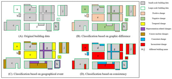
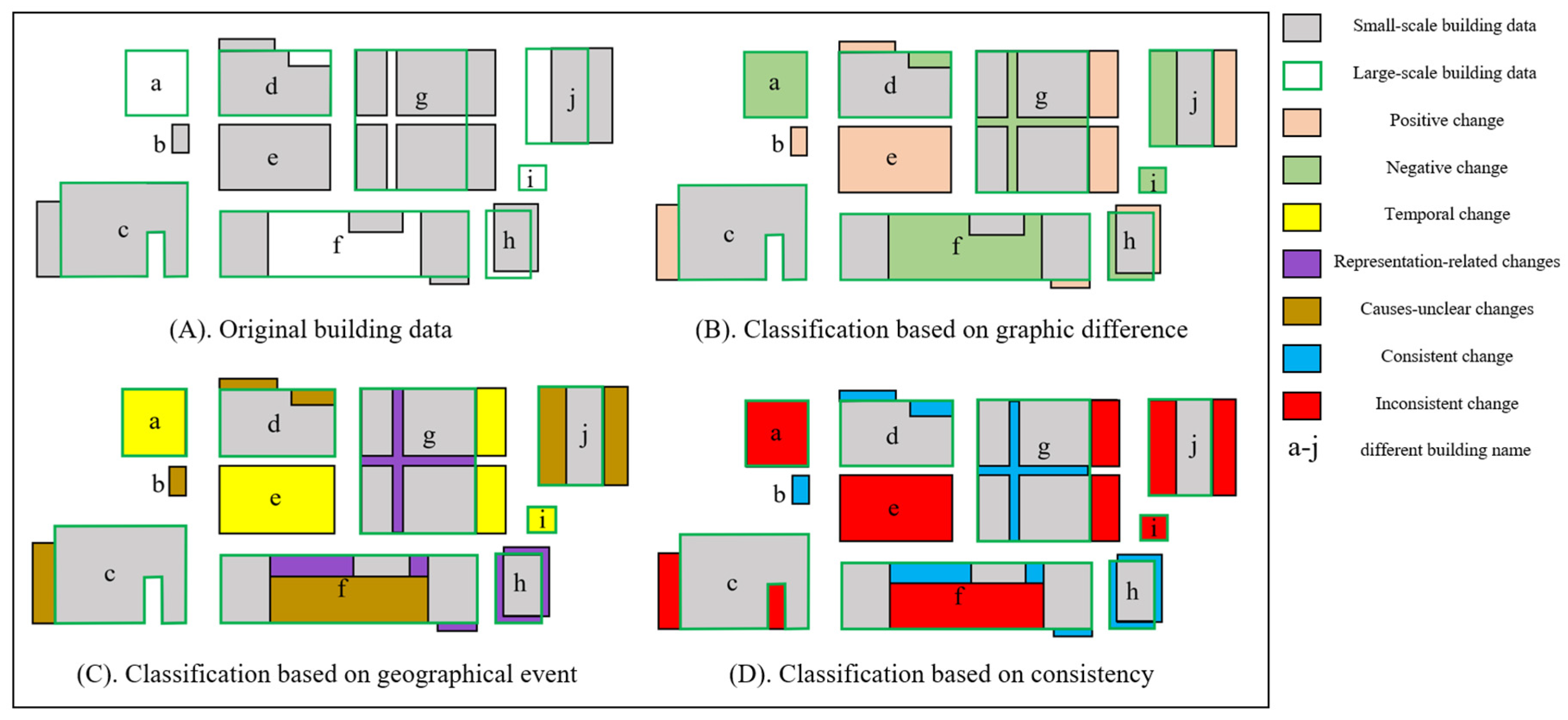
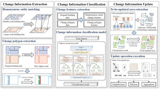
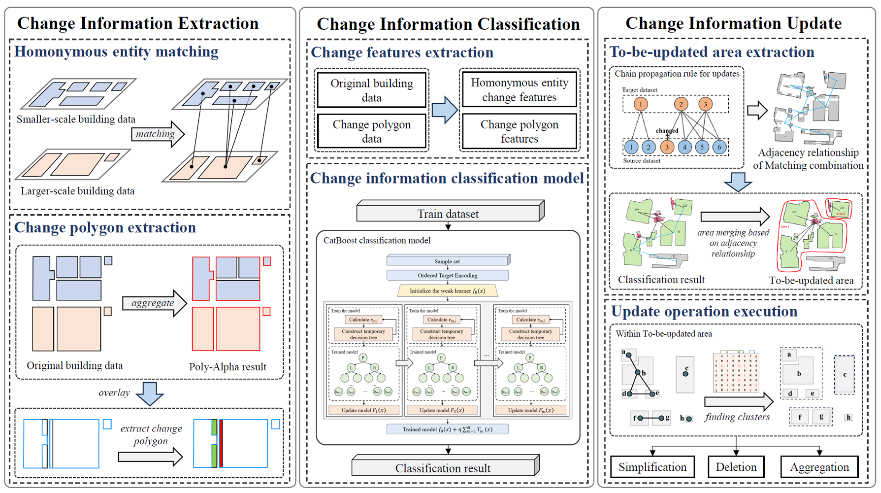
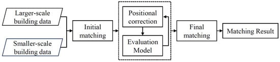
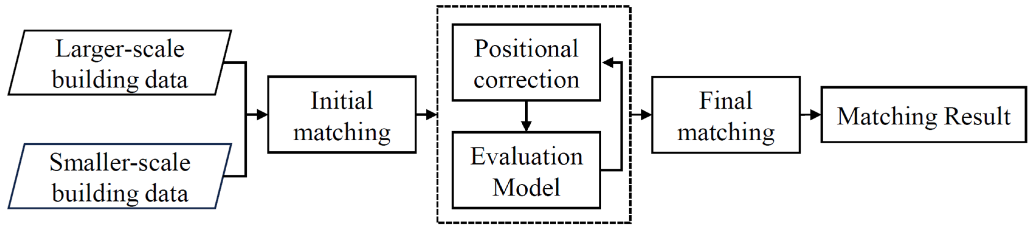
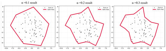
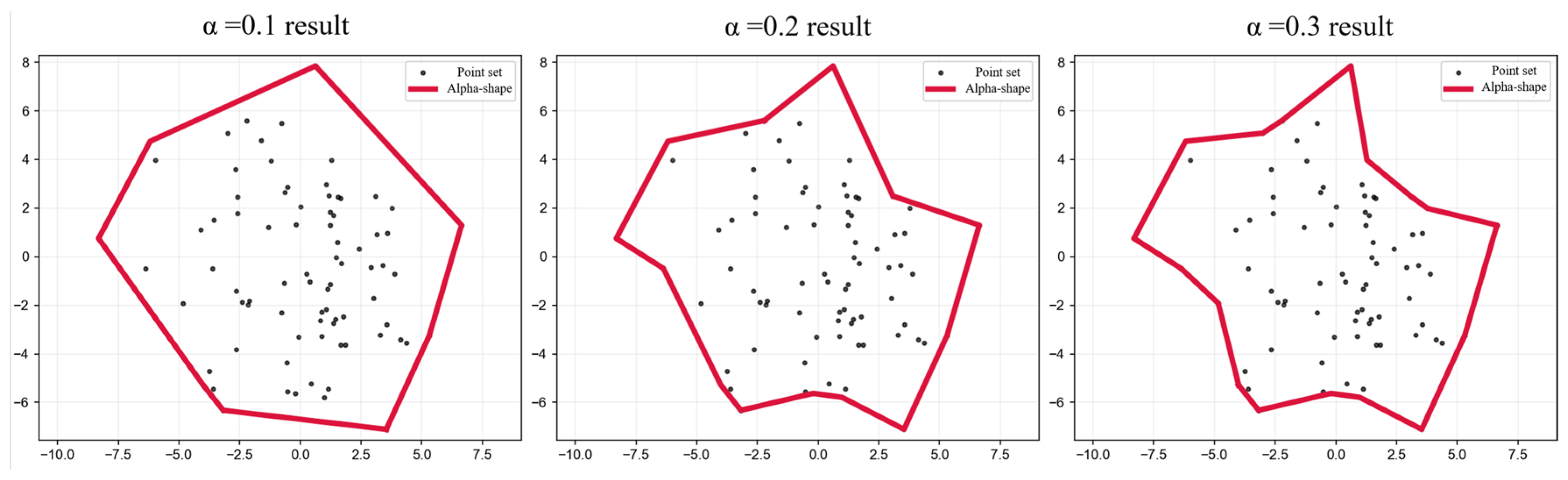
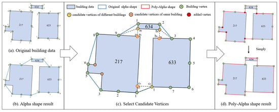
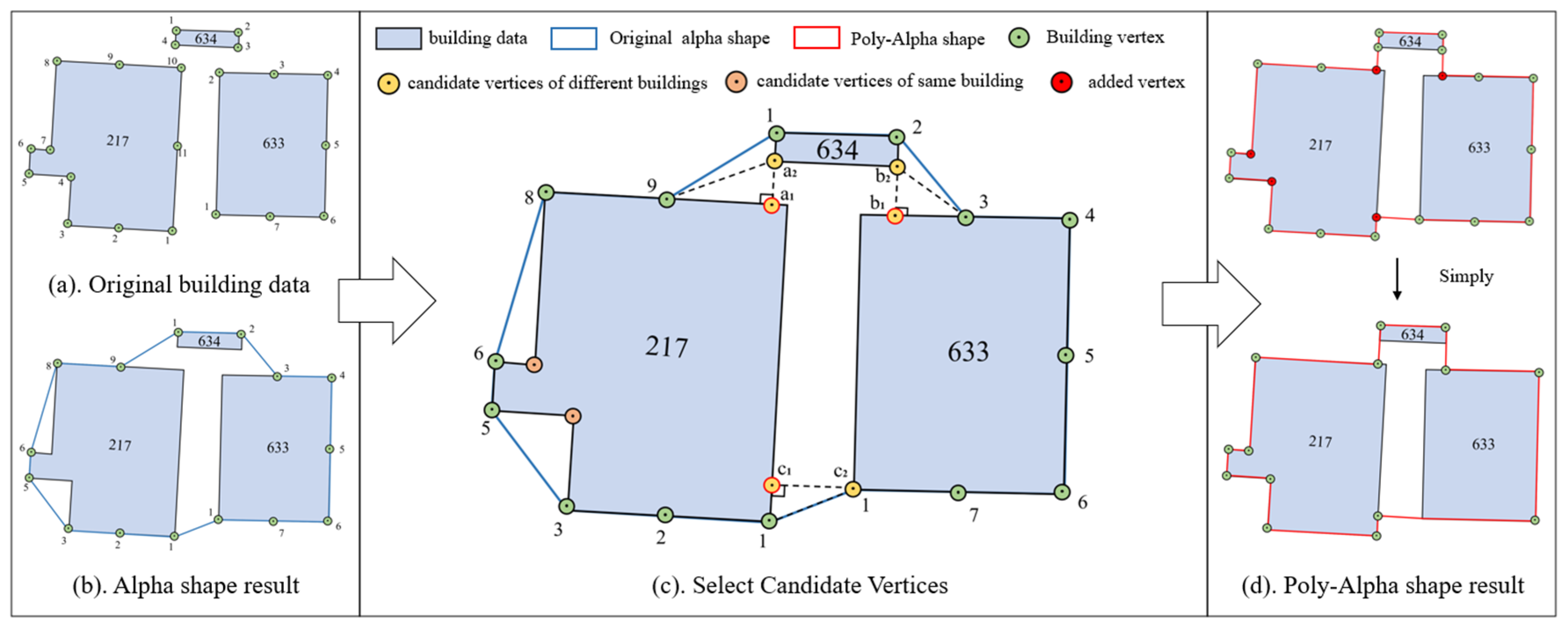
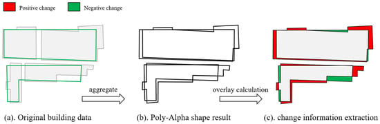
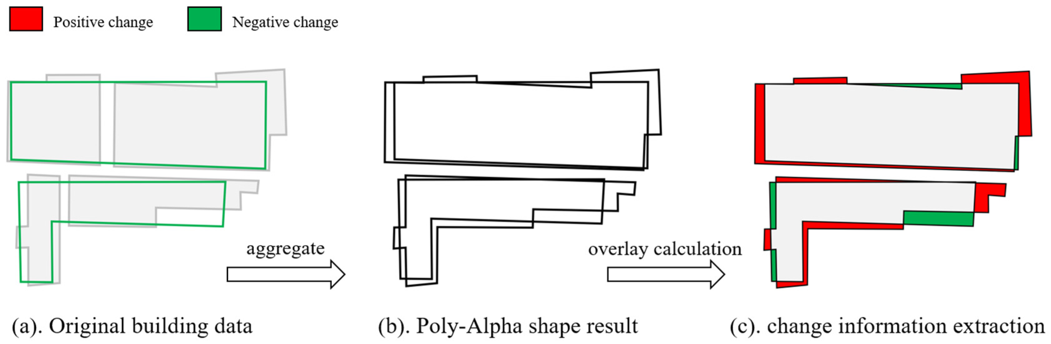
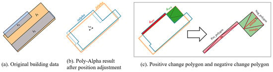
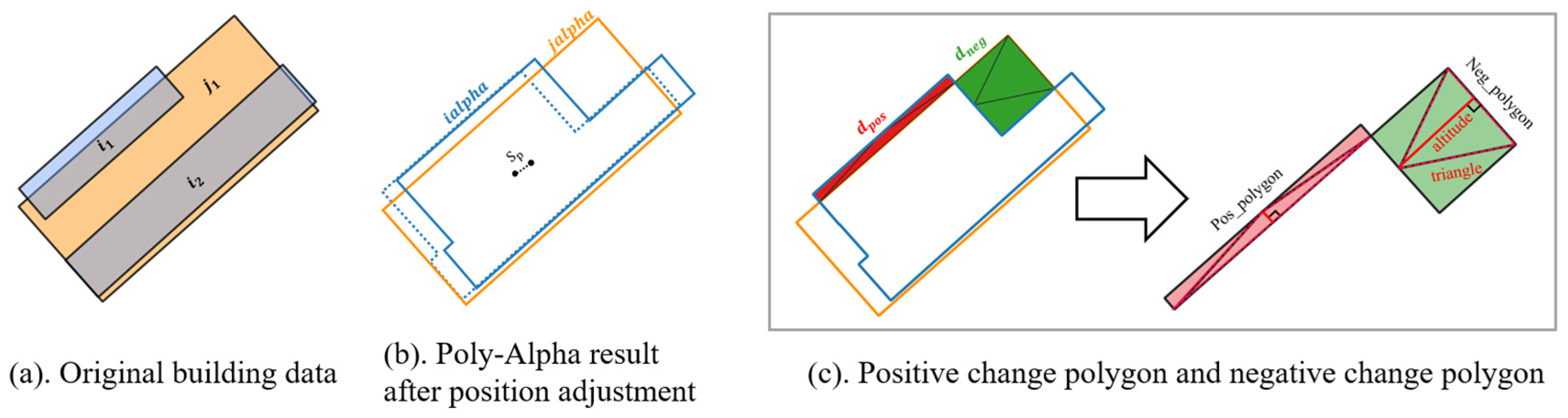
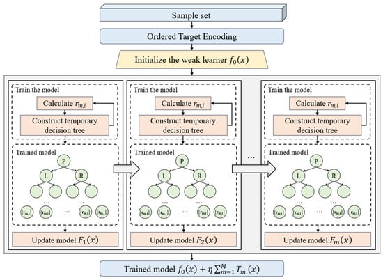
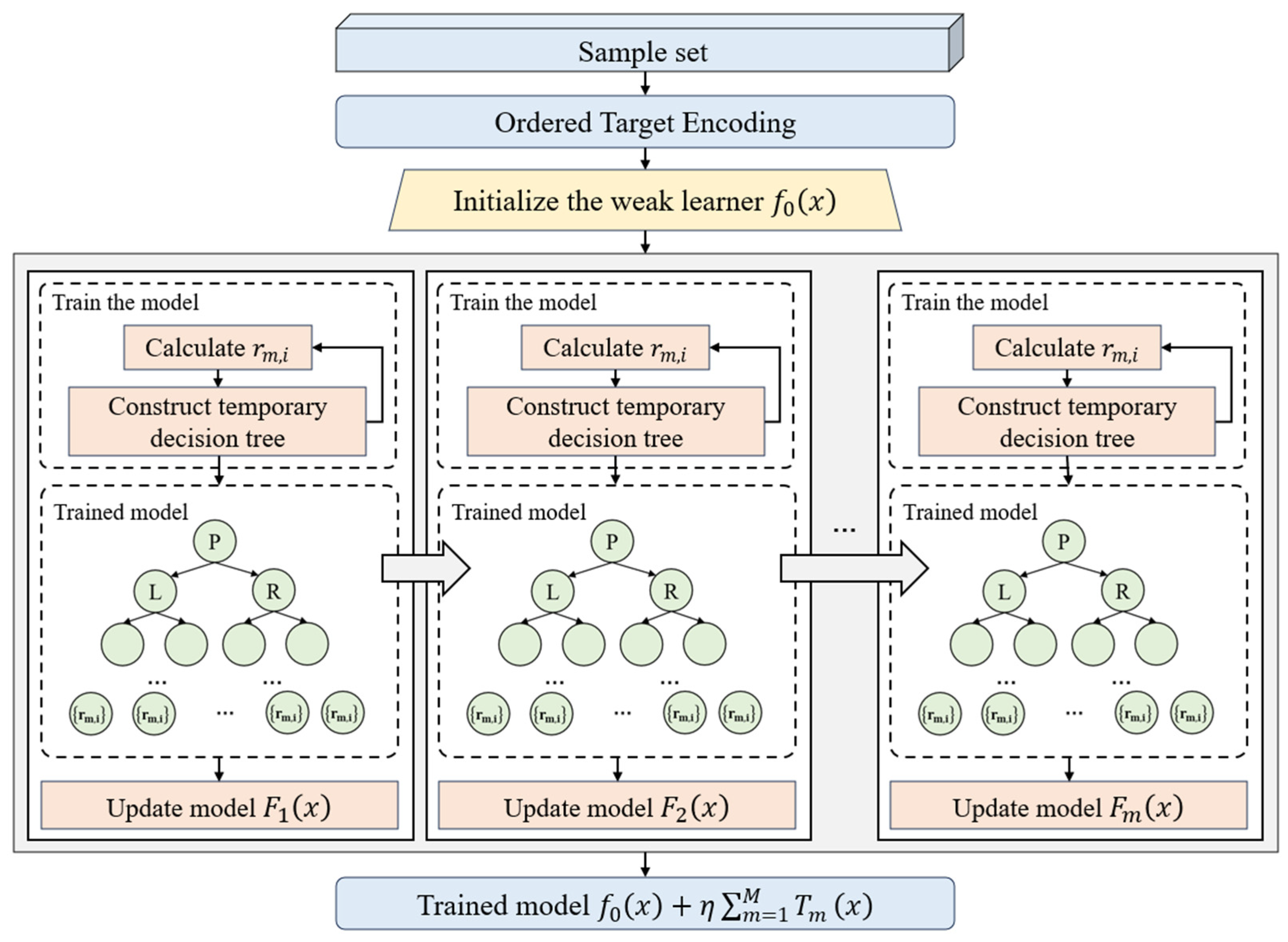
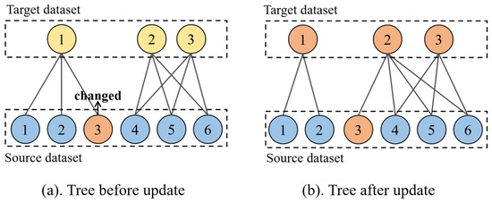
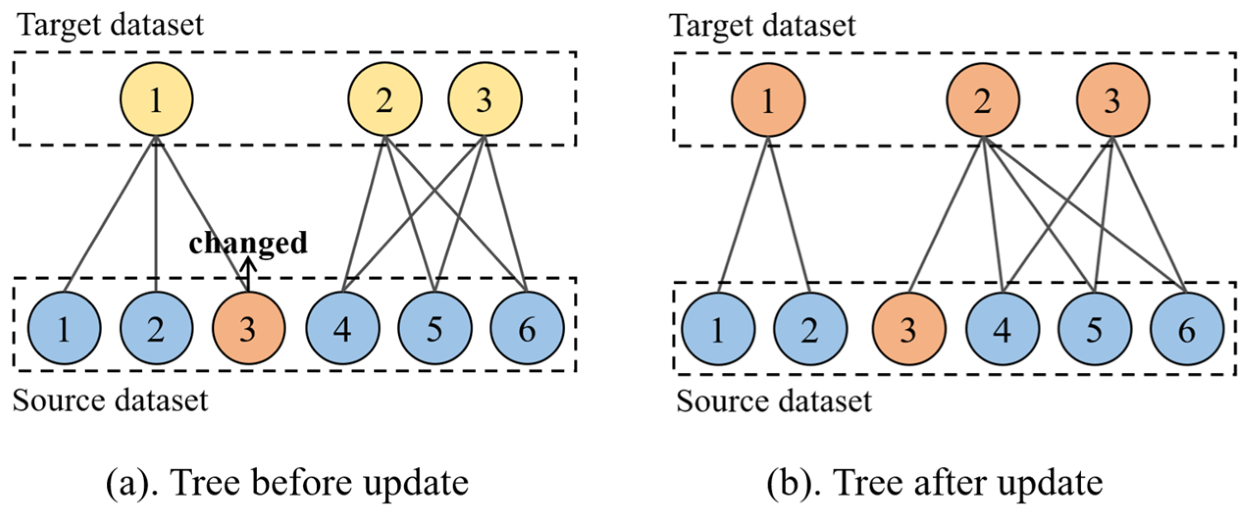
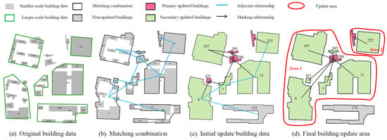
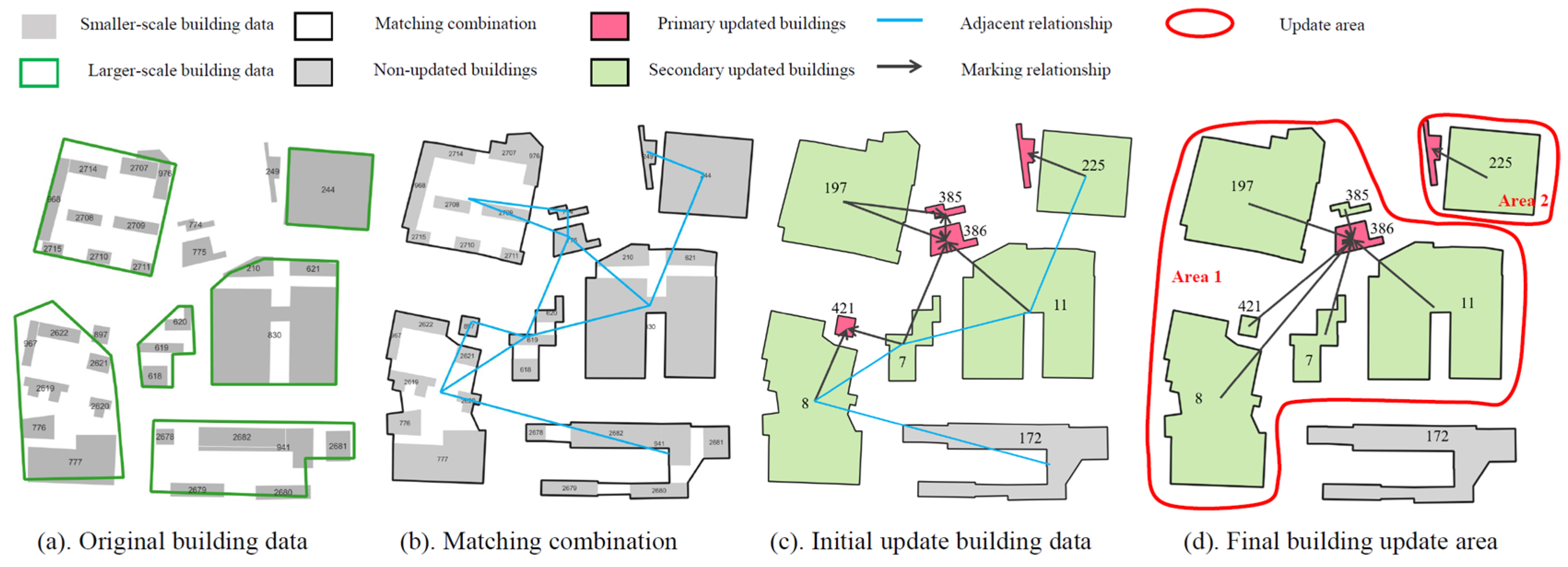
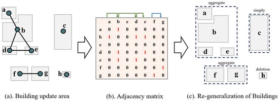
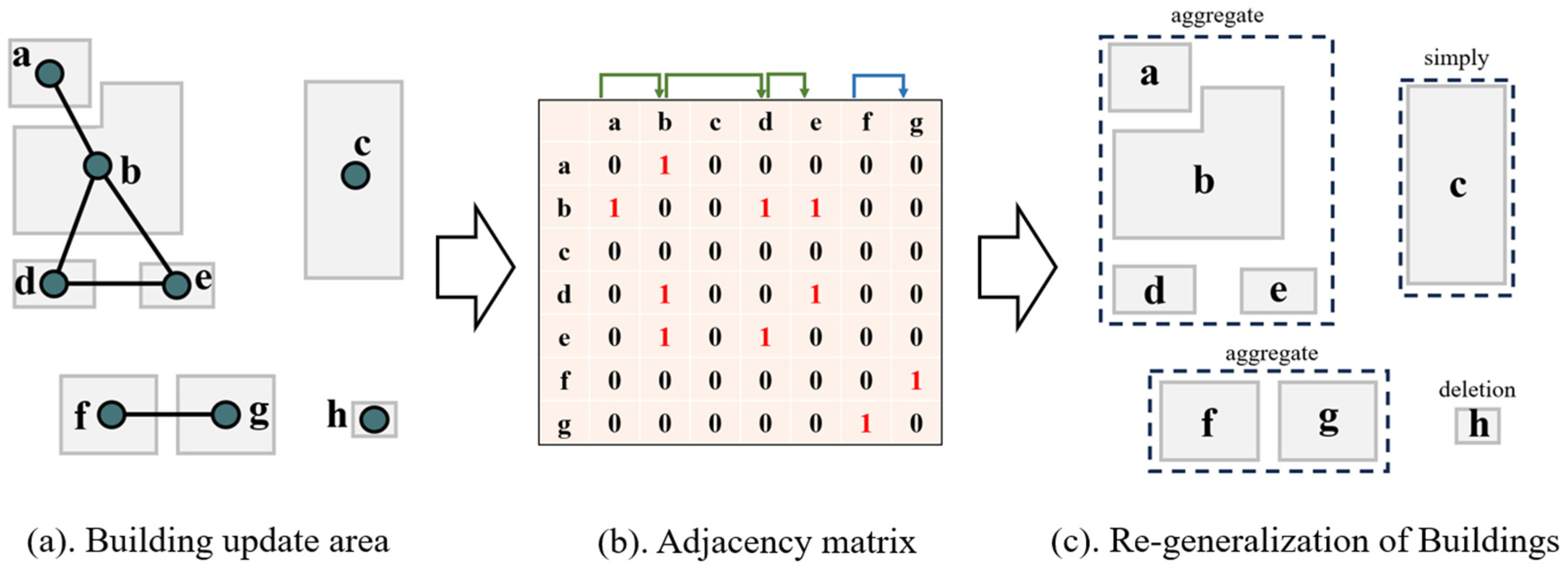
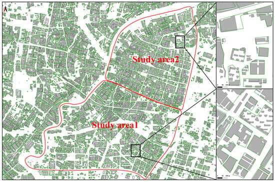
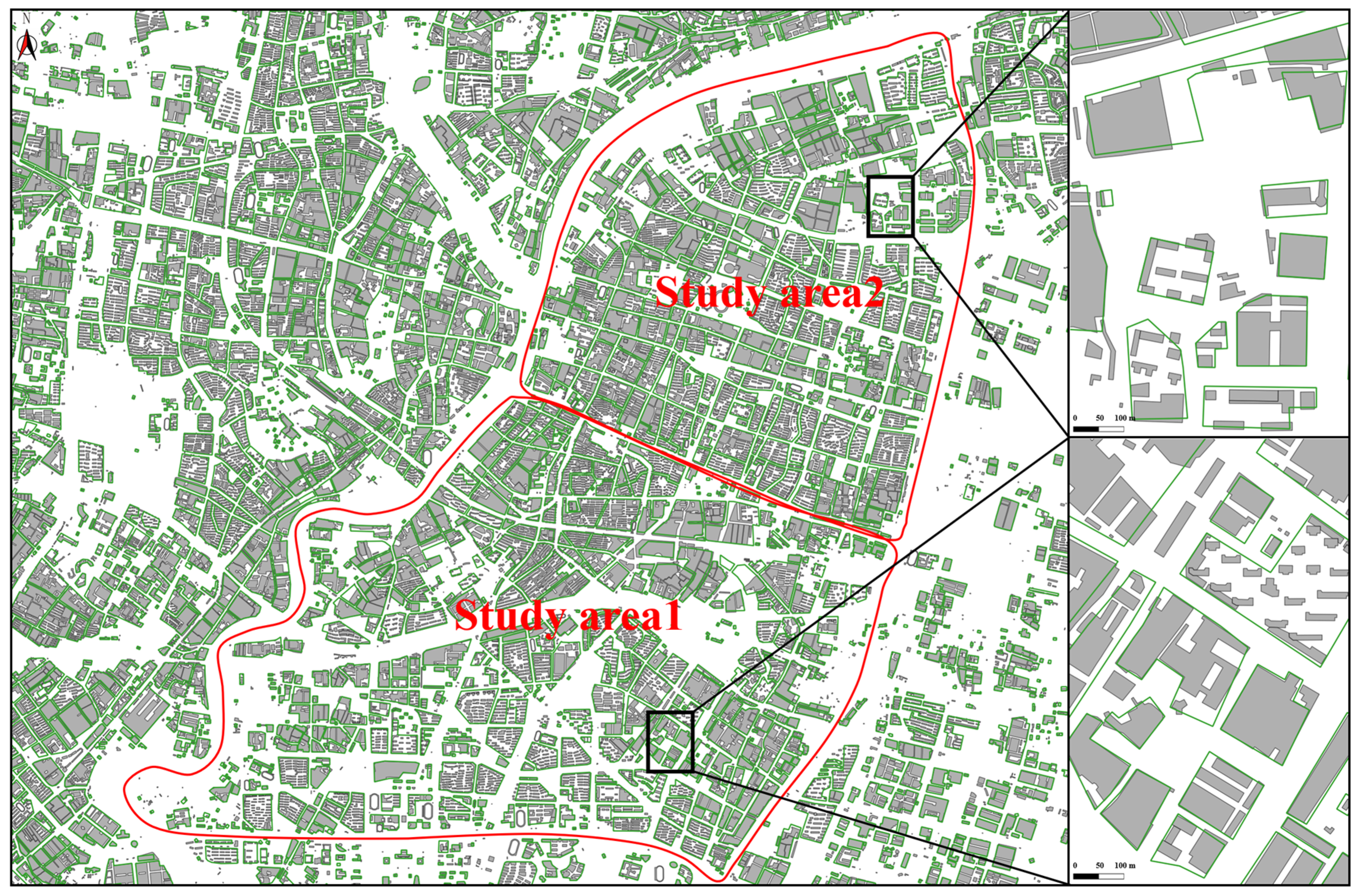
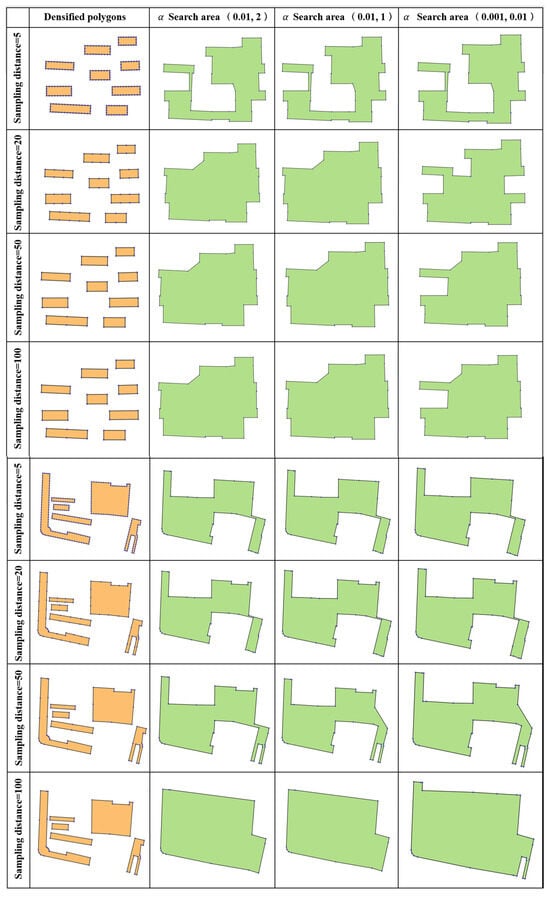
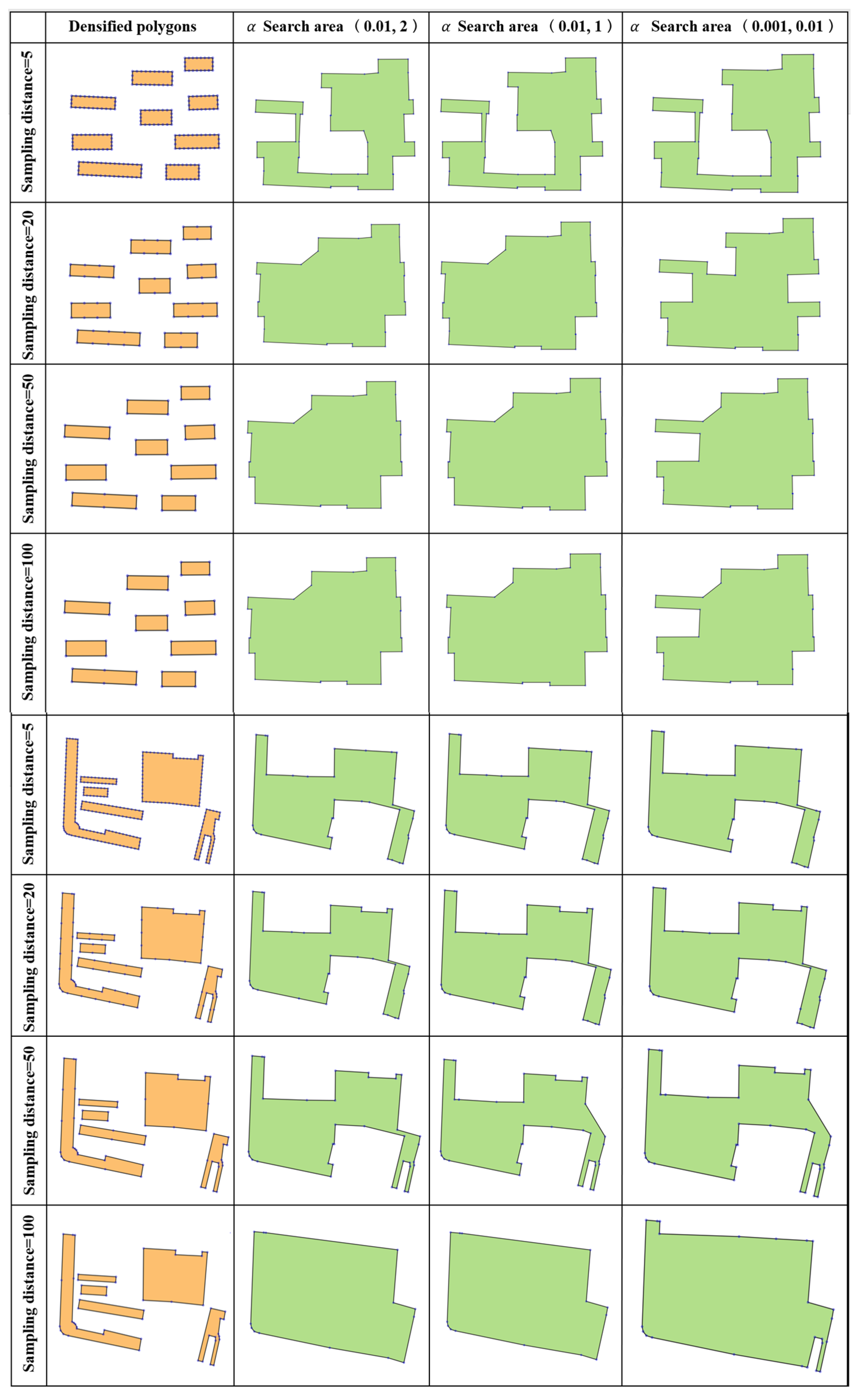
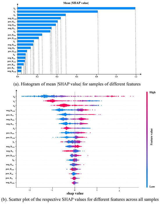
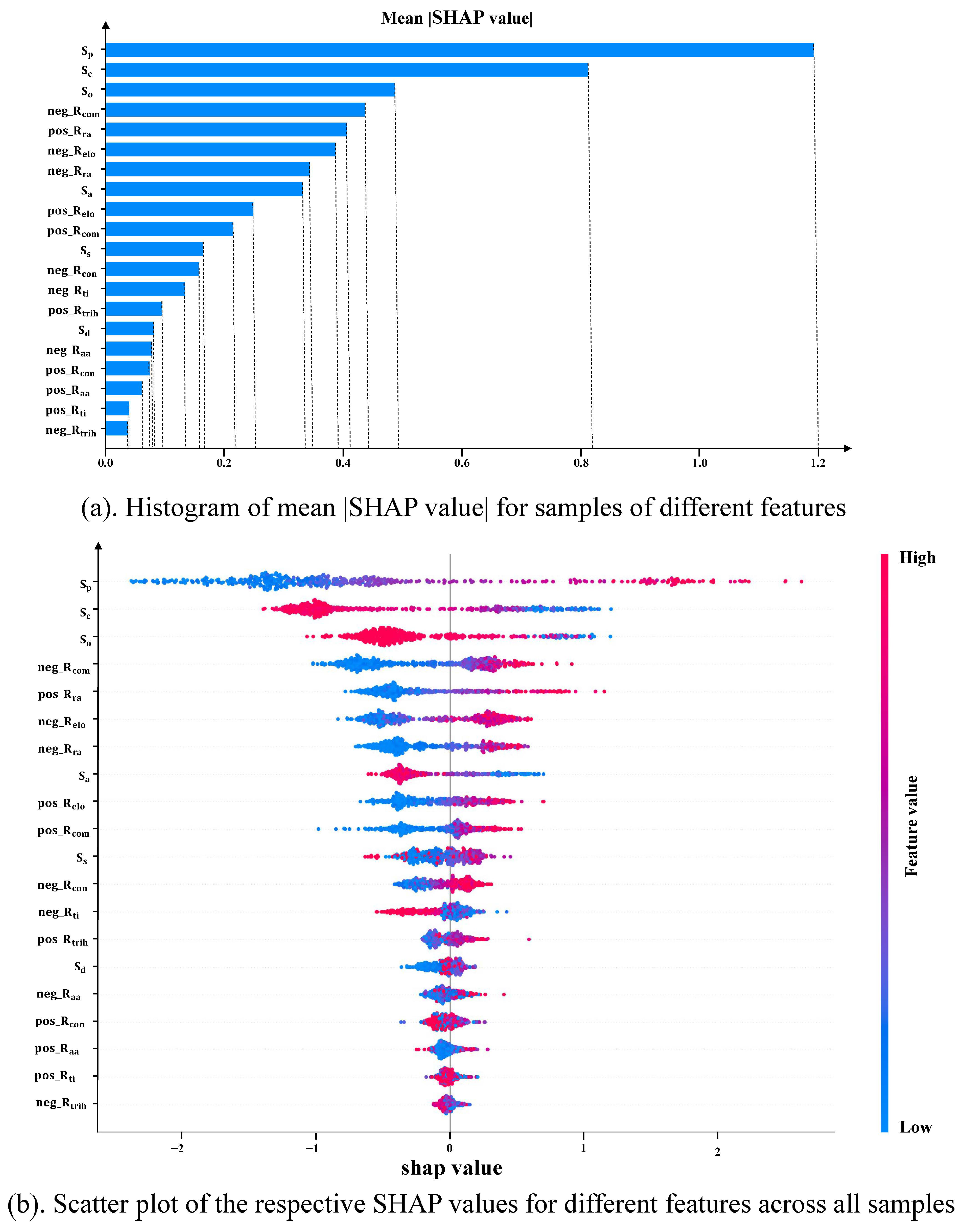
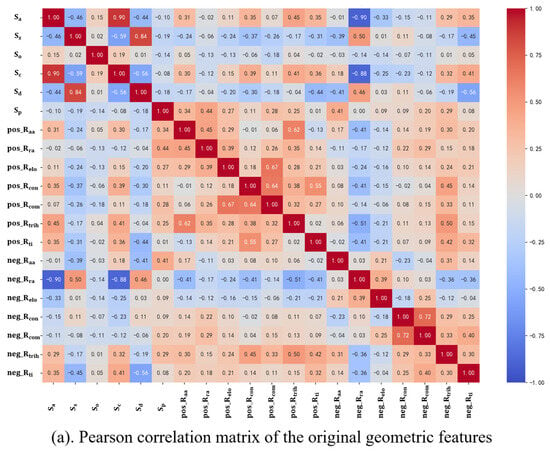
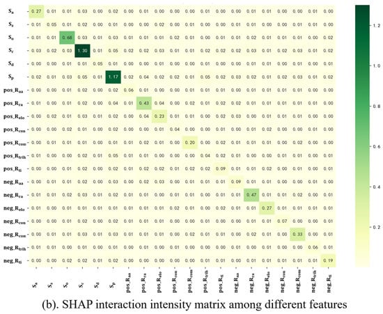
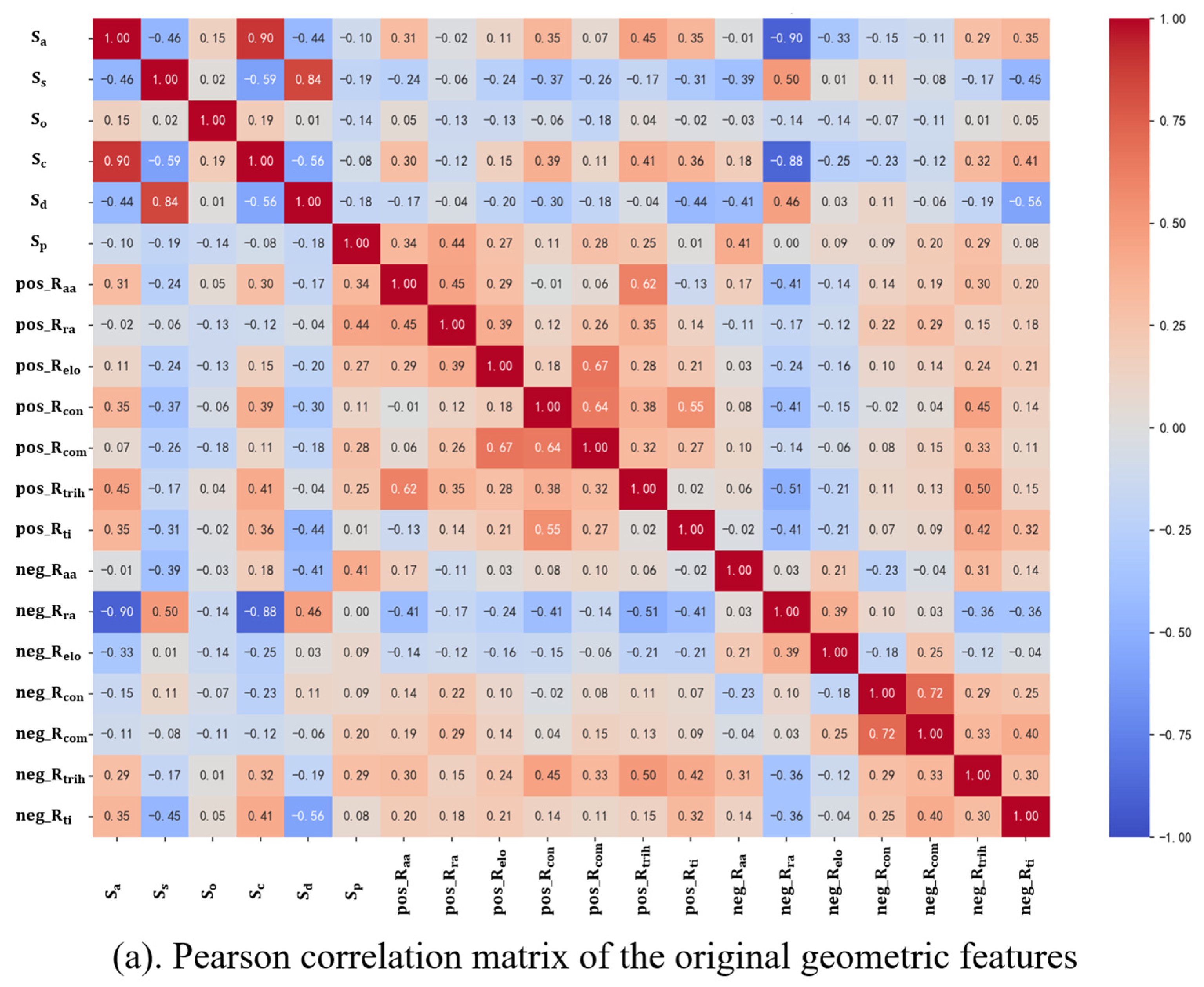
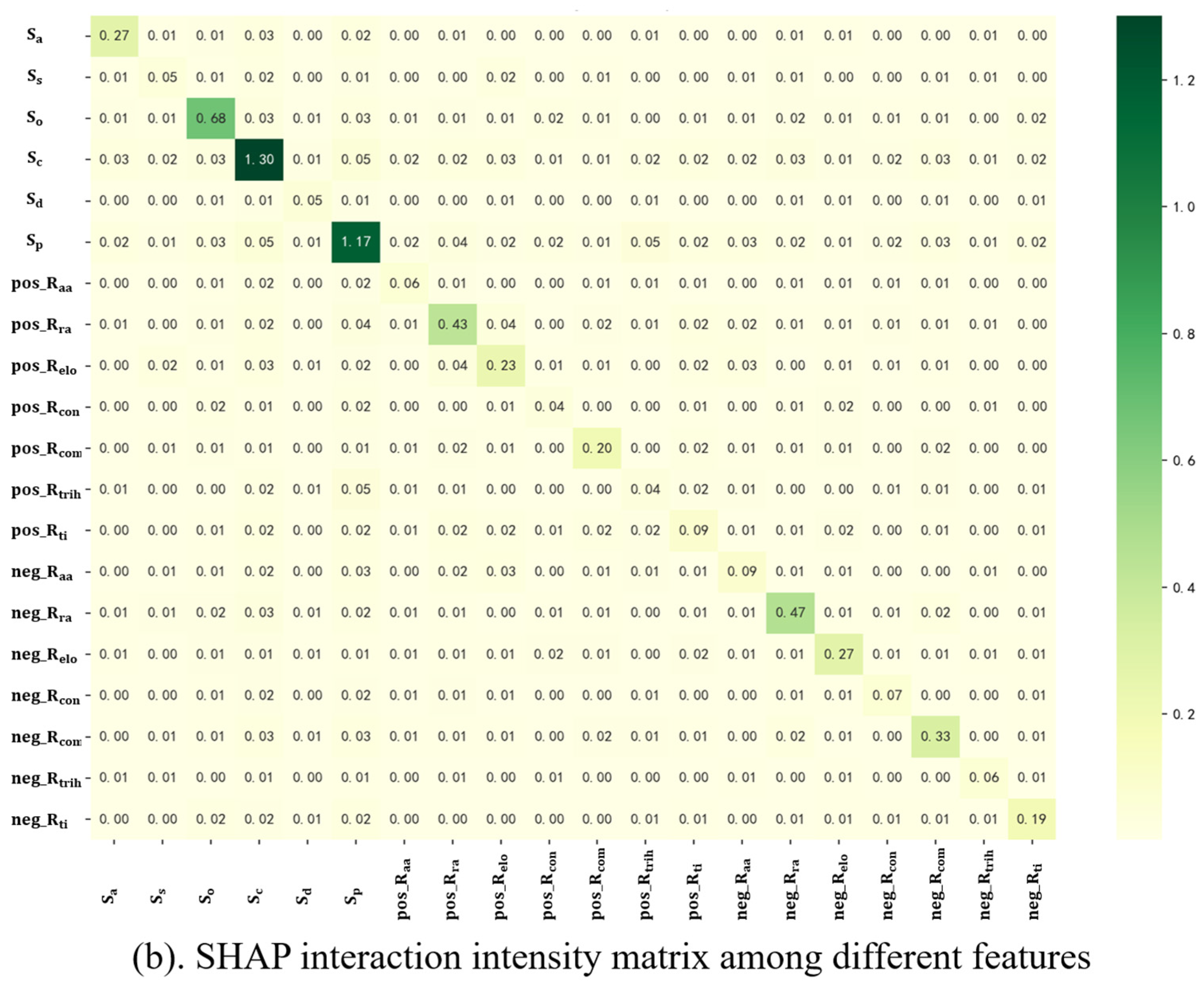
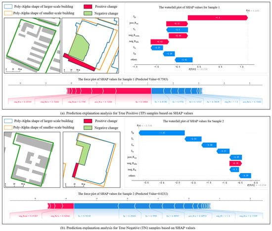
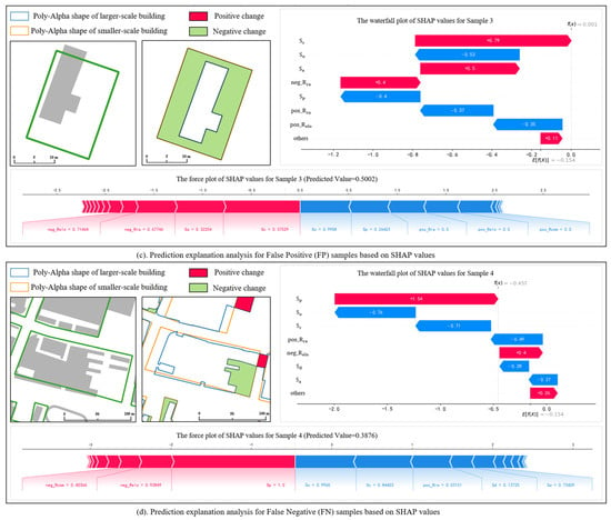
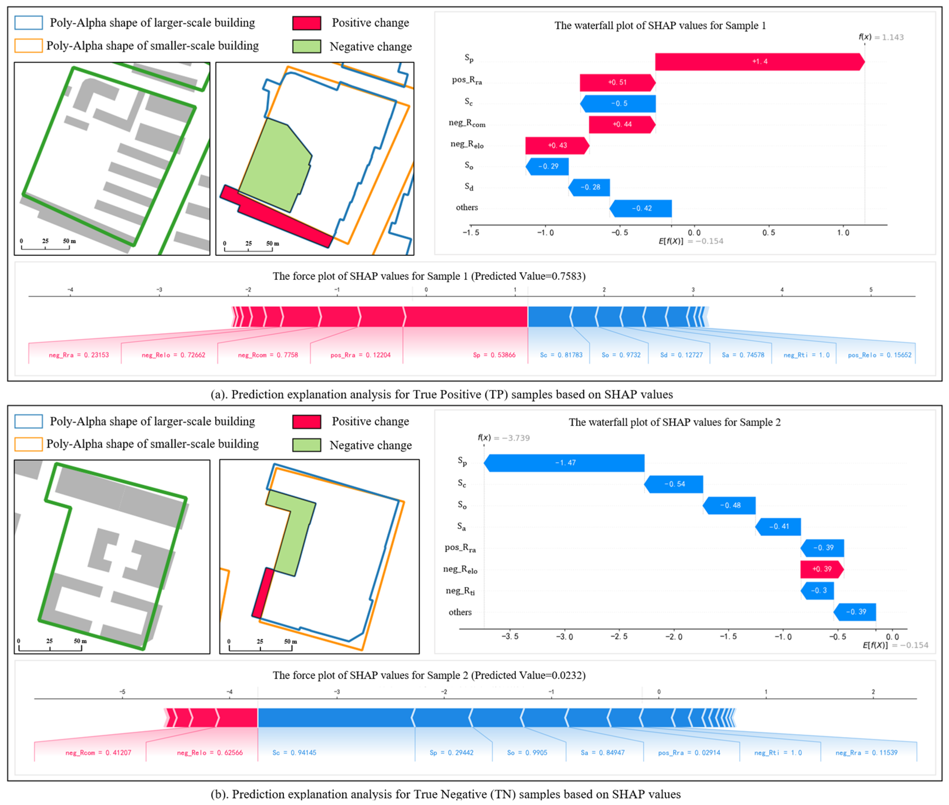
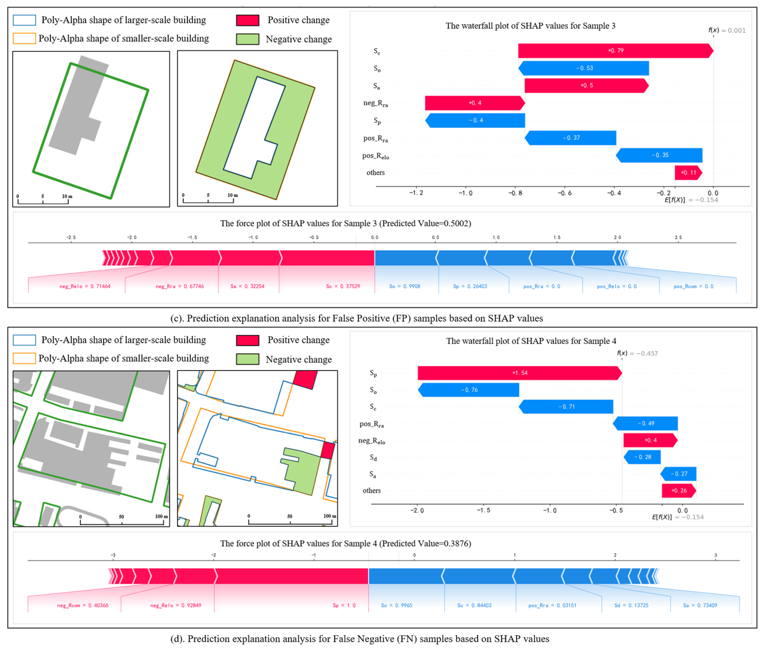
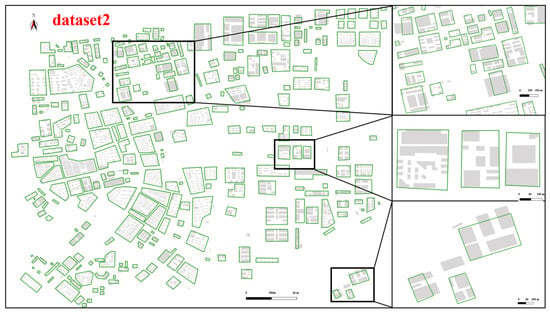
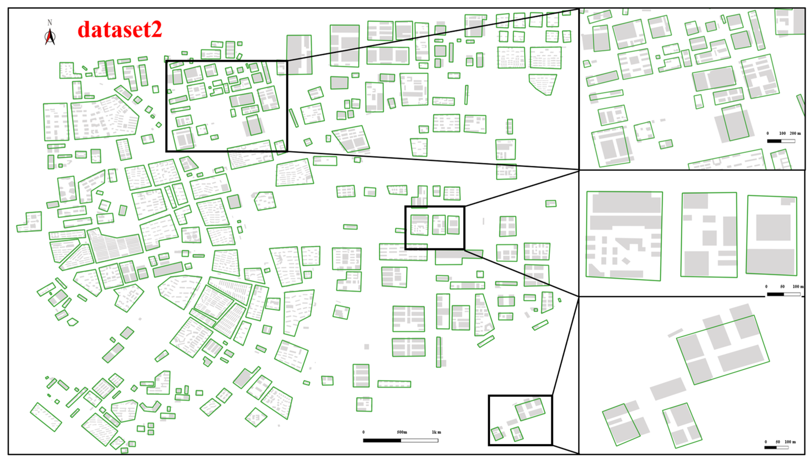
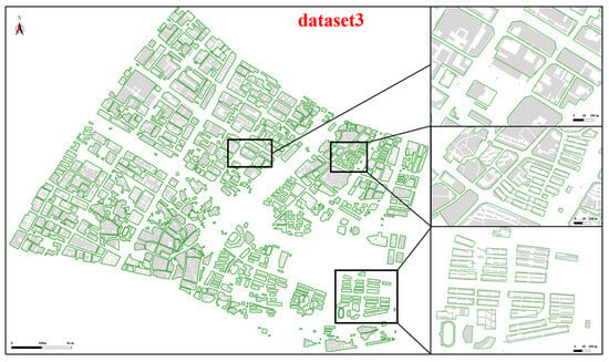
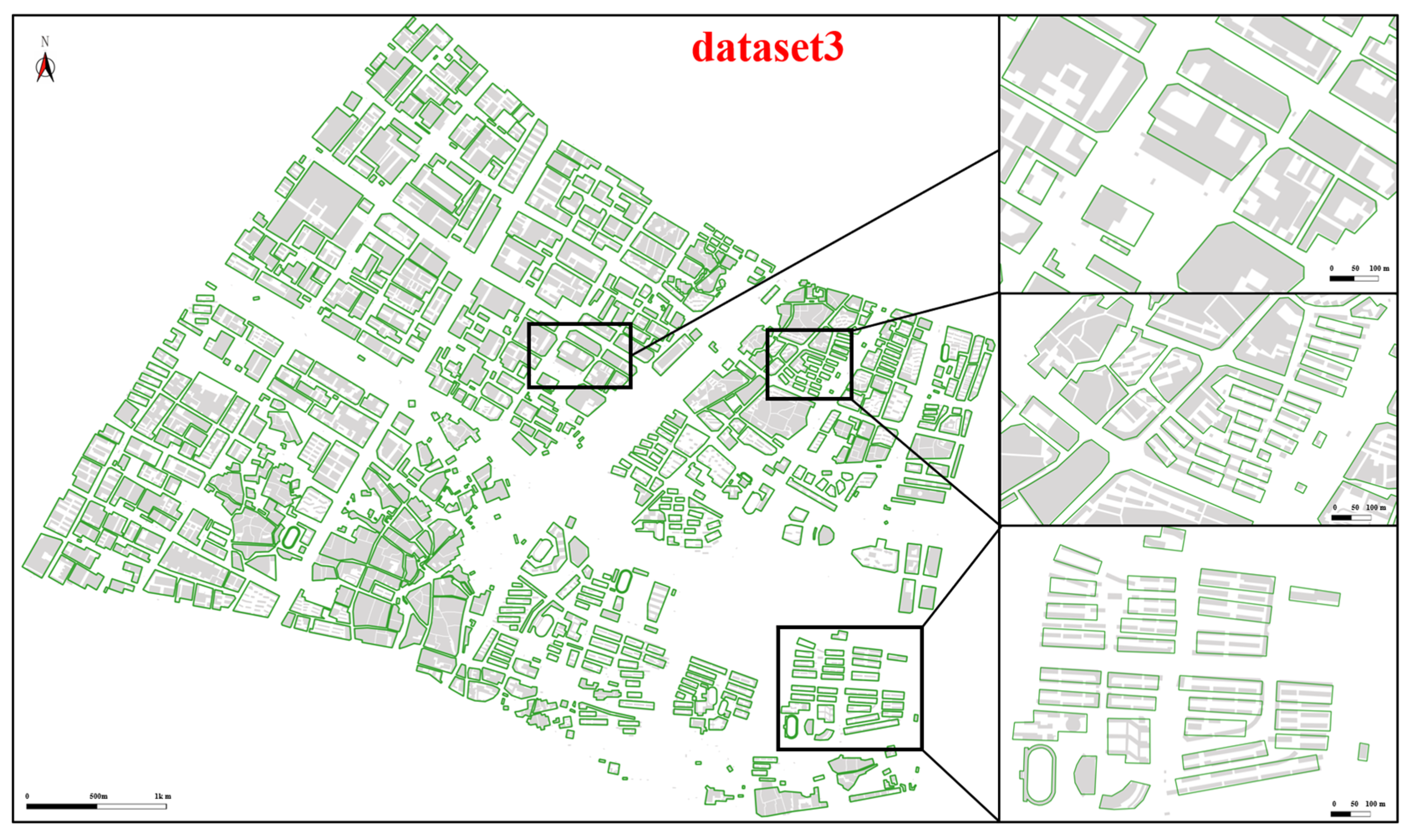
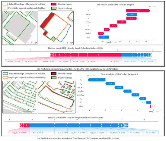
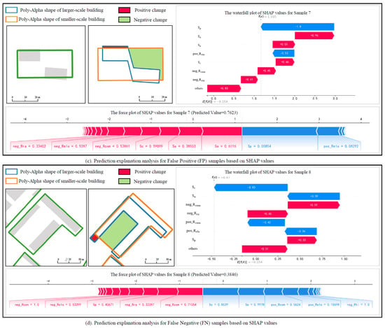
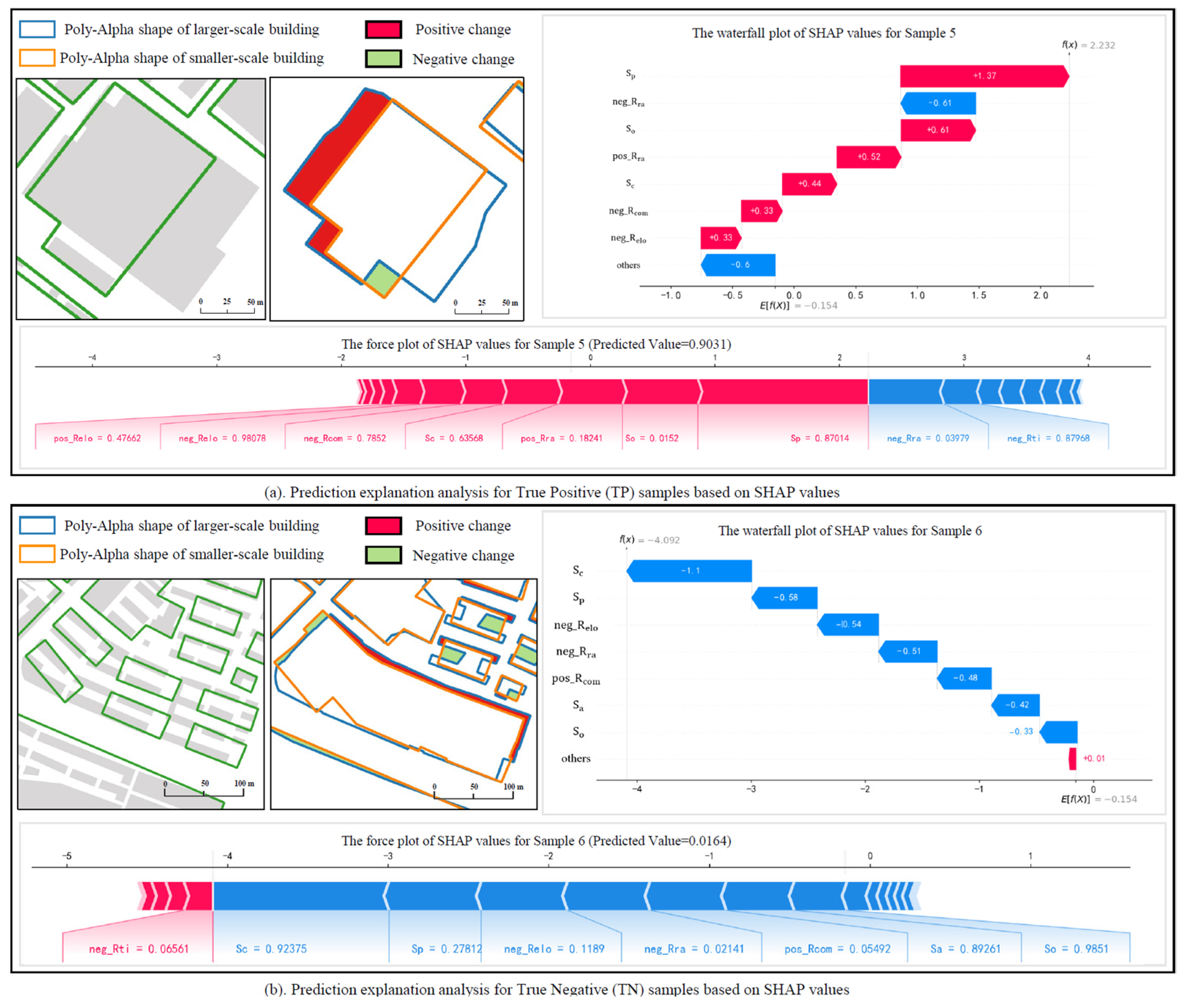
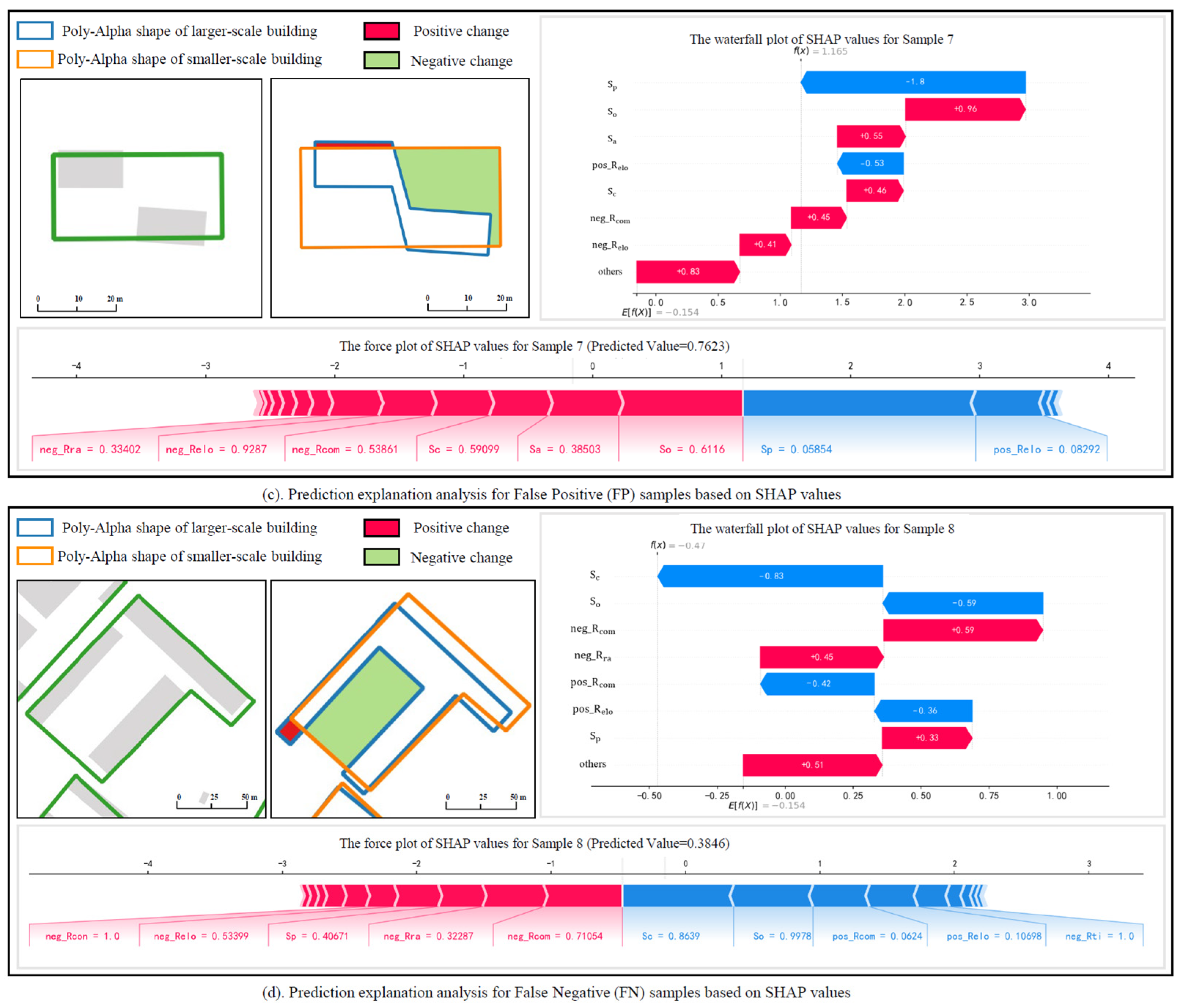
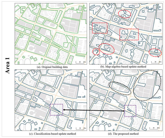
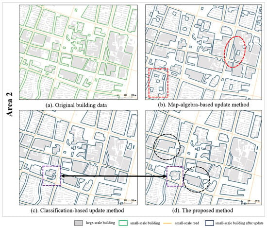
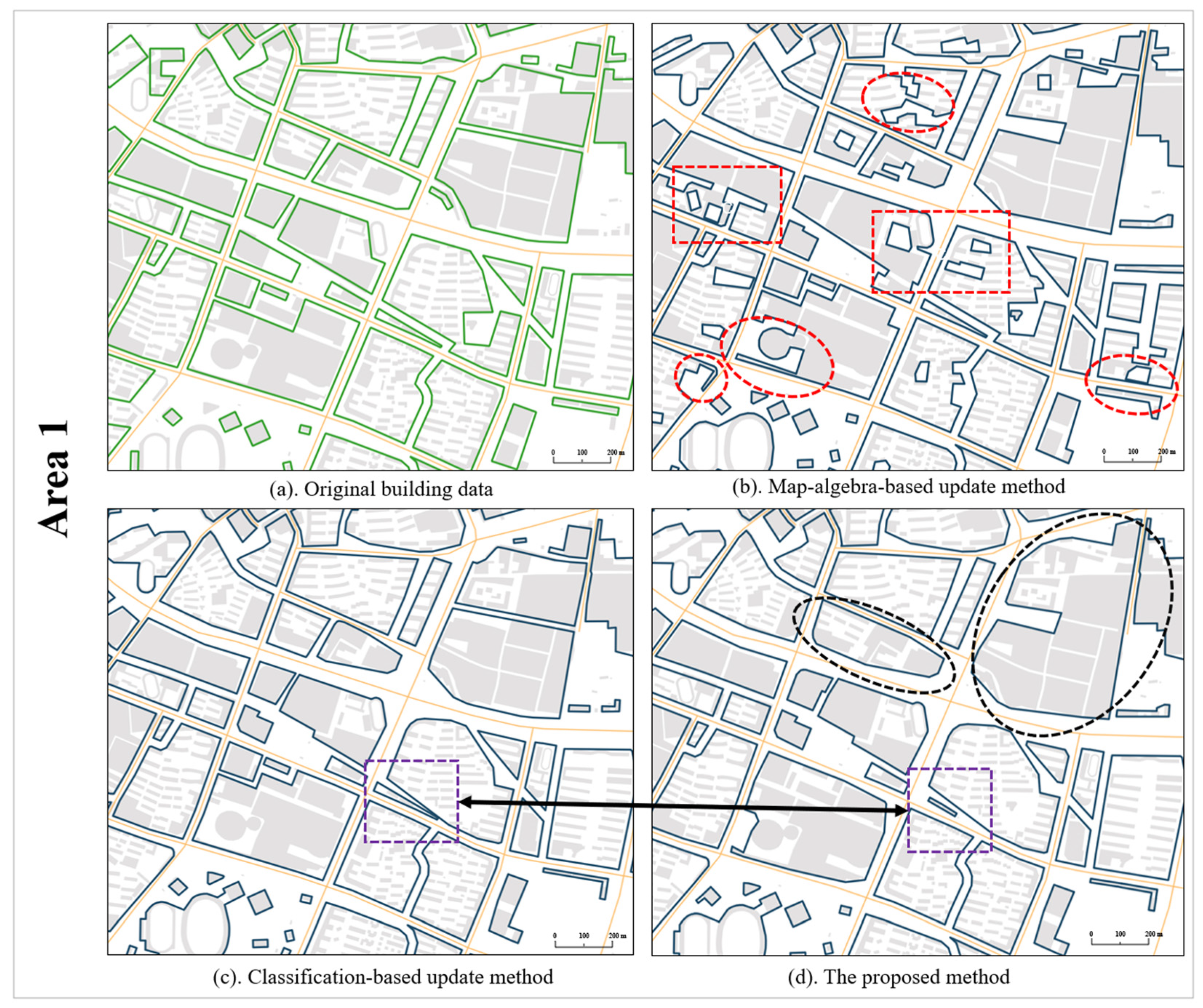
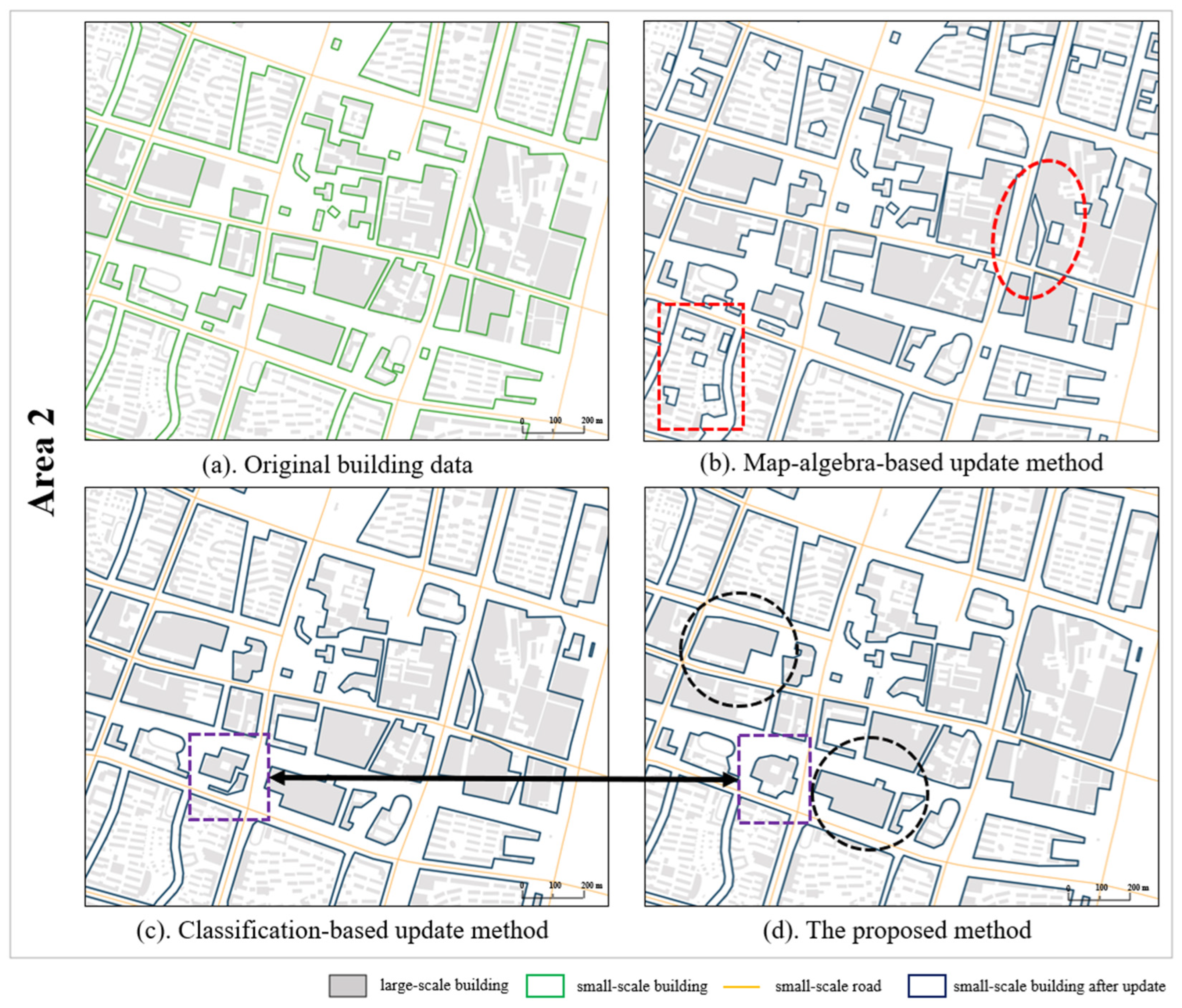
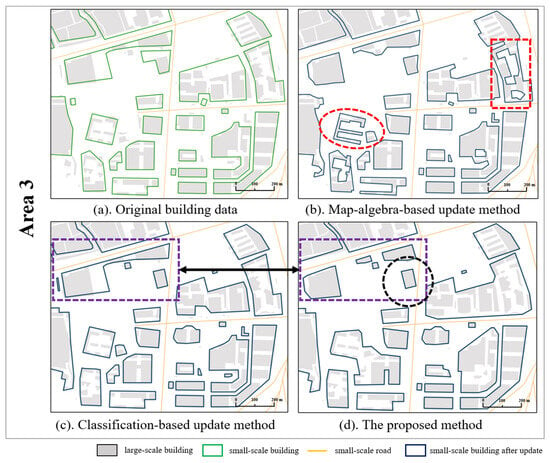
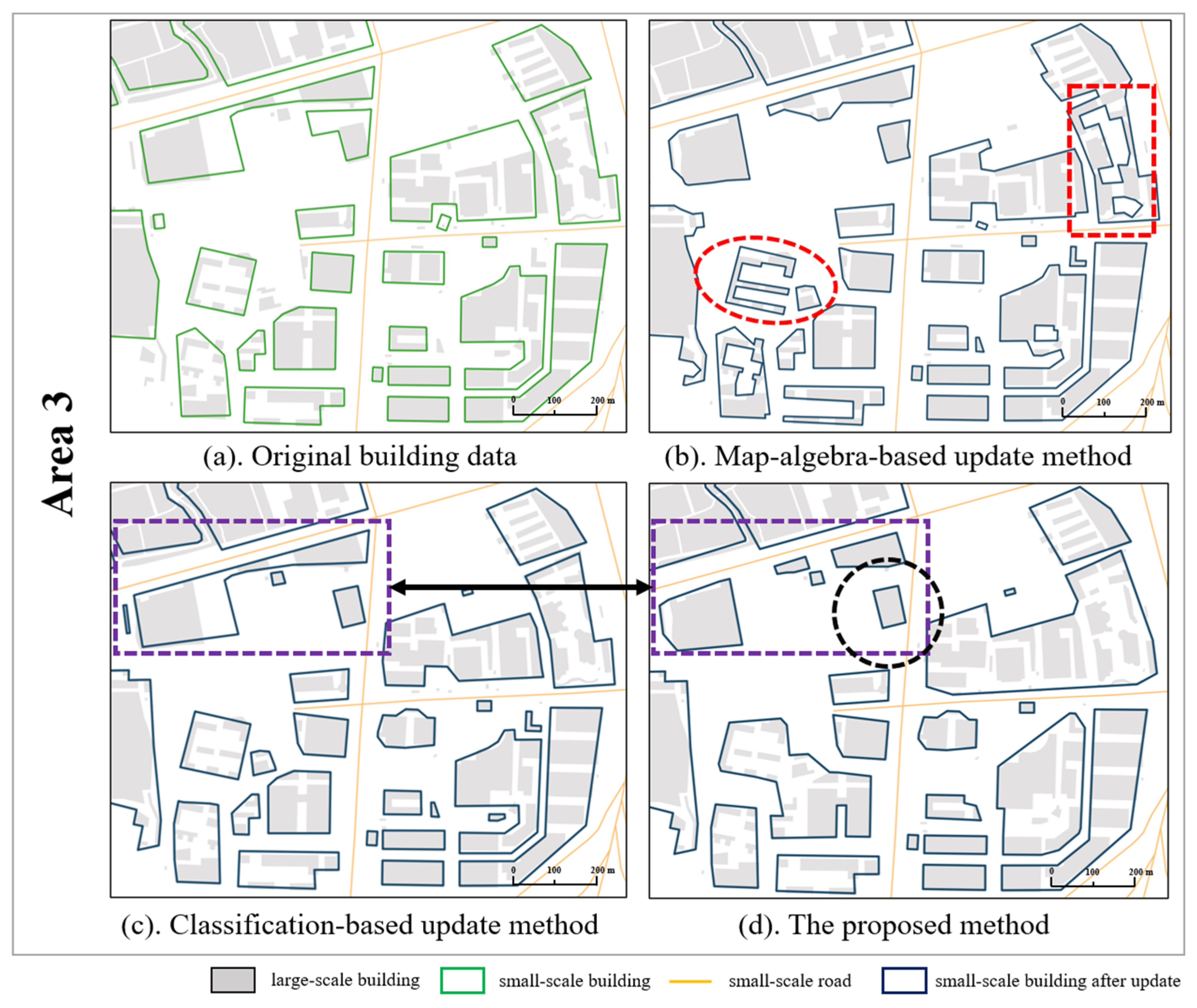

Disclaimer/Publisher’s Note: The statements, opinions and data contained in all publications are solely those of the individual author(s) and contributor(s) and not of MDPI and/or the editor(s). MDPI and/or the editor(s) disclaim responsibility for any injury to people or property resulting from any ideas, methods, instructions or products referred to in the content. |
© 2026 by the authors. Published by MDPI on behalf of the International Society for Photogrammetry and Remote Sensing. Licensee MDPI, Basel, Switzerland. This article is an open access article distributed under the terms and conditions of the Creative Commons Attribution (CC BY) license.